69
Background Material: Markov Decision Process
| Date post: | 21-Dec-2015 |
| Category: |
Documents |
| View: | 221 times |
| Download: | 0 times |

Background Material: Markov Decision Process
Reference
Class notes
Further studies:
Dynamic programming and Optimal Control
D. Bertsekas, Volume 1
Chapters 1, 4, 5, 6, 7

Discrete Time Frameworkxk System State belongs to set Sk
uk Control Action belongs to set U(xk ) Ck
wk Random Disturbance characterized by a probability distribution Pk (./ xk , uk ) which may depend on xk , uk but not on values of prior disturbances w0 ……wk-1
xk+1 = fk (xk , uk , wk )
N Number of times control is applied
gk (xk , uk , wk ) Cost in slot k
gN (xN) Terminal Cost

Finite Horizon ObjectiveChoose the controls such that additive expected cost over N time slots is minimized, that is minimize
E{gN (xN) + k=0N-1 gk (xk , uk , wk ) }
Control strategy:
= {w0 = 0(x0) …wN-1 = N-1(xN-1)… }
Cost associated with control and initial state x0
J (x0) = Ew {gN (xN) + k=0N-1 gk (xk , uk , wk ) }
Choose such that J (x0) is minimized for all initial states x0
Optimal controls need only be a function of the current state (history independence)
Type of Control
Open loopCan not change in response to system statesOptimal if disturbance is a deterministic function of the state and the control
Closed loop
Can change in response to system states
Illustrating Example: Inventory Control
xk Stock available at the beginning of the kth period
Sk Set of integers
uk Stock ordered at the beginning of the kth period
U(xk ) =Ck Set of nonnegative integers
wk Demand during the kth period characterized by a probability distribution Pk (wk), w0 ……wN-1 which are independent
xk+1 = xk + uk - wk
Negative stock: Backlogged Demand
N Time horizon of optimization

gk (xk , uk , wk ) Cost in slot k consists of two components
Penalty for storage and unfulfilled demands r(xk )
Ordering cost cxk
gk (xk , uk , wk ) = cxk + r(xk )
gN (xN) = r(xN) Terminal Cost for being left with inventory xN
Example Control action (Threshold type)
uk = k - xk if xk < k
= 0 otherwise

Bellmans Principle of Optimality
Let the optimal strategy be * = {0* ……..N-1*} Assume that a
given state x occurs with a positive probability at time j. Let the system be in state x in slot j, then the truncated control sequence {i
* ……..N-1*} minimizes the cost to go from slot j to N, that is minimizes Ew {gN (xN) + k=j
N-1 gk (xk , uk , wk ) }

Dynamic Programming Algorithm
Optimal algorithm is given by the following iteration which proceeds backwards
JN (xN) = gN (xN)
Jk(xk) = minu in U(x) Ew { gk (xk , uk , wk ) + Jk (xk+1) }
= minu in U(x) Ew { gk (xk , uk , wk ) + Jk (fk (xk , uk , wk ) ) }

Optimizing a Chess Match Strategy
A player plays against an opponent who does not change his actions in accordance with the current state
They play N games,
If the scores are tied towards the end, then the players go to sudden death, where they play until one is ahead of the other
A draw fetches 0 point for both, a win fetches 1 point for the winner and 0 for the loser
The player can play timid, in that case draws a match with probability pd and loses with probability (1- pd )
The player can play bold, in that case wins a match with probability pw and loses with probability (1- pw )
Optimal strategy in sudden death?
Play bold

Optimal Strategy in initial N games
xN Difference between the score of the player and his opponent
Sk integers between k and -k
uk Timid (0) or Bold (1)
U(xk ) = {0, 1}
wk Outcome: Probability distribution for timid {pd , 1- pd}
Probability distribution for bold {pw , 1- pw}
xk+1 = wk
N Time horizon of optimization

Consider maximization of reward instead of minimization of cost
gN (xN) = 0 if xN < 0
= pw if xN = 0
= 1 if xN > 0
gk (xk , uk , wk ) is the probability of winning in k games
gk (xk , uk , wk ) = 0 if k < N
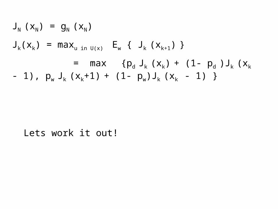
JN (xN) = gN (xN)
Jk(xk) = maxu in U(x) Ew { Jk (xk+1) }
= max {pd Jk (xk) + (1- pd )Jk (xk - 1), pw Jk (xk+1) + (1- pw)Jk (xk - 1) }
Lets work it out!

State Augmentation
What if system state depends not only on the preceding state and control, but also earlier state and control?
xk+1 = fk (xk , uk , xk-1 , uk-1 , wk ), x1 = f1 (x0 , u0 , w0 )
Now state is (xk , yk , sk )
xk+1 = fk (xk , yk , sk , uk , wk ),
yk+1 = xk
sk+1 = uk Time lag in cost

Correlated Disturbances
What if w0 …wN-1 are not independent?
Let wj depend on wj-1
state is (xk , yk , sk )
xk+1 = fk (xk , yk , uk , wk ),
yk+1 = wk

Linear Systems and Quadratic Cost
xk+1 = Ak xk + Bk uk + wk,
gN (xN) = xNT QNxN
gk (xk) = xkT Qkxk + uk
T Rkuk
k(xk) = Lk xk
Lk = - (BkT Kk+1Bk + Rk )-1
BkT Kk+1Ak
KN = QN
Kk = - AkT(Kk+1 - Kk+1Bk (Bk
T Kk+1Bk + Rk )-1 Bk
T Kk+1 )Ak + Qk

J(x0) = x0T K0x0 + k=0
N-1 E(wkT Kk+1wk)
optimum cost
Let Ak = A,, Bk = B, Rk = R, Qk = Q
Then as k becomes large, Kk converges to the steady state solution of algebraic Ricatti equation,K = - AT(K - KB (BT KB + R )-1
BT K )A + Q
(x) = L x
L = - (BTKB + R)-1 BT KA

Optimal Stopping Problem
One of the control actions allow the system to stop in any slot
Decision maker can terminate the system at a certain loss or choose to continue at a certain cost.
The challenge will be when to stop so as to minimize the total cost.

Asset selling problemA person has an asset for which he receives quotes in every slot, w0 …wN-1
Quotes are independent from slot to slot
If a person accepts the offer, he can invest it at a fixed rate of interest r > 0
Control action is to sell or not to sell
State is the offer in the previous slot if the asset is not sold yet, or T if it is sold
xk+1 = T if sold in previous slots
= wk otherwise
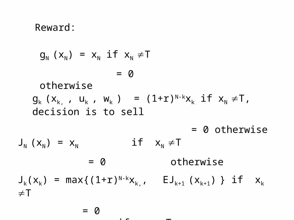
Reward:
gN (xN) = xN if xN T
= 0 otherwise
gk (xk, , uk , wk ) = (1+r)N-kxk if xN T, decision is to sell
= 0 otherwise
JN (xN) = xN if xN T
= 0 otherwise
Jk(xk) = max{(1+r)N-kxk,, EJk+1 (xk+1) } if xk T
= 0 if xN = T

Let k = EJk+1 (wk)/ (1+r)N-k
Optimal strategy: Accept the offer if xk > k
Reject the offer if xk < k
Act either way otherwise
To show k is non-increasing function of k
We will show by induction that Jk+1 (x)/ (1+r)N-k is non-increasing for all x
JN (x)/ (1+r) = x/(1+r)
JN-1 (x)/ (1+r)2 = max(x/(1+r), EJN (xk+1))
Thus JN (x) )/ (1+r) JN-1 (x)/ (1+r)2 , base case holds

Jk(x)/ (1+r)N-k+1 = max{(1+r)-1x, EJk+1 (w)/ (1+r)N-k+1 }
Jk+1(x)/ (1+r)N-k = max{(1+r)-1x, EJk+2 (w)/ (1+r)N-k }
By induction, Jk+1 (w)/ (1+r)N-k+1 Jk+2 (w)/ (1+r)N-k
The result follows
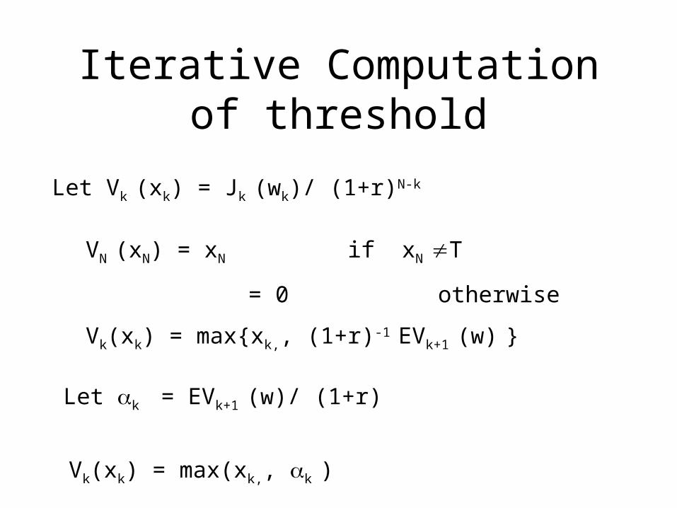
Iterative Computation of threshold
Let Vk (xk) = Jk (wk)/ (1+r)N-k
VN (xN) = xN if xN T
= 0 otherwise
Vk(xk) = max{xk,, (1+r)-1 EVk+1 (w) }
Let k = EVk+1 (w)/ (1+r)
Vk(xk) = max(xk,, k )

Let k = EVk+1 (w)/ (1+r)
=E max(w,, k ) )/ (1+r)
= (0 to k+1 k+1 dP + k+1 to infty wdP) )/ (1+r)
P is the cumulative distribution function of w
Note that the first and the last parts are upperbounded
k is a decreasing sequence
For large k, the sequence converges to where
Let = (0 to dP + to infty wdP) )/ (1+r)

General Stopping Problem
Decision maker can terminate the system in slot k at a certain cost t(xk)
Terminal cost is t(xN)
JN (xN) = t(xN )
Jk(xk) = min{t(xk),, minu in U(x) E {g(xk, , uk , wk ) + Jk+1 (f(xk,u,w))} }
Optimal to stop at time k for states x in the set S such that
Tk = {t(x), minu in U(x) E {g(x , u , w ) + Jk+1 (f(x,u,w))} }

We show by induction that Jk (x) is non-decreasing in k
I
It follows that T0 T1 …..TN-1
Assume that TN-1 is an absorbing set that is, if a state is in this set, and termination is not selected then the next state is also in this set.
Consider a state x in TN-1
Note that JN-1 (x) = t(x )
minu in U(x) E {g(x, , u , w ) + JN-1 (f(x,u,w)) } = minu in U(x) E {g(x,,u ,w ) + t (f(x,u,w)) }
= minu in U(x) E {g(x,,u ,w ) + t(x)} t(x)
JN-2 (x) = t(x).

Thus x is in TN-2. Thus TN-1. TN-2
Similarly TN-1 …..T1 T0
Thus TN-1 = …..T1 = T0
The optimal decision is to stop once the state is in a certain stopping set, and this set does not depend on the iteration number.
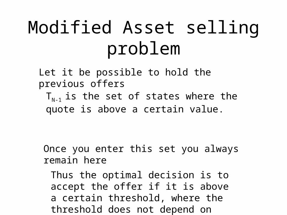
Modified Asset selling problem
Let it be possible to hold the previous offers
TN-1 is the set of states where the quote is above a certain value.
Once you enter this set you always remain here
Thus the optimal decision is to accept the offer if it is above a certain threshold, where the threshold does not depend on the iteration.

Multiaccess Communication
A bunch of terminals share a wireless medium.
Only one user can successfully transmit a packet at a time.
A terminal attempts a packet with a probability which is a function of the total queue length in the system.
Multiple attempts cause interference, no attempt causes poor utilization.
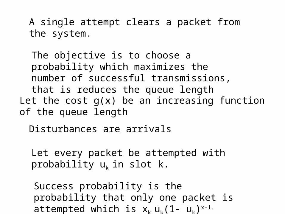
A single attempt clears a packet from the system.
The objective is to choose a probability which maximizes the number of successful transmissions, that is reduces the queue length
Let the cost g(x) be an increasing function of the queue length
Let every packet be attempted with probability uk in slot k.
Success probability is the probability that only one packet is attempted which is xk uk(1- uk)x-1. Refer to it as p(xk ,uk)
Disturbances are arrivals

Jk(xk) = gk (xk) + minu in [0, 1] Ew { p(xk , uk ) Jk+1 (xk+ wk - 1)
= + (1 - p(xk , uk )) Jk+1 (xk + wk ) }
= gk (xk) + Jk+1 (xk + wk ) + minu in [0,1] Ew { p(xk , uk ) (Jk+1
(xk+ wk - 1) - Jk+1 (xk + wk ) )}
Jk(x) is an increasing function of x for each k since gk(x) is an increasing function of x.
Thus Jk (xk+ wk) Jk (xk + wk - 1)
The minimum is attained if p(xk , uk ) is maximized.
Happens when uk = 1/ xk
Every terminal needs to know the entire queue length which is not realistic

Imperfect State Information
System has access to imperfect information about the state x, that is now the observation is zk and not xkwhere
zk is now hk (xk , uk-1 , vk ), where vk is a random disturbance which may now depend on the entire history
Choose the controls such that additive expected cost over N time slots is minimized, that is minimize
E{gN (xN) + k=0N-1 gk (xk , uk , wk ) }
xk+1 = fk (xk , uk , wk )

Reformulation as a perfect state problem
Let Ik be the vector of all previous observations and controls.
Consider Ik as the system state now.
Ik+1 = (Ik , uk , zk+1 )
JN-1(xk) = minu E{gN (fN ( xN-1 , uN-1 , wN-1 )) + gN-1 (xN-1 , uN-
1 , wN-1 ) | IN-1 , uN-1 }
Jk(Ik) = minu E{gk ( xk , uk , wk ) + Jk+1 (Ik , zk+1 , uk ) | Ik , uk }
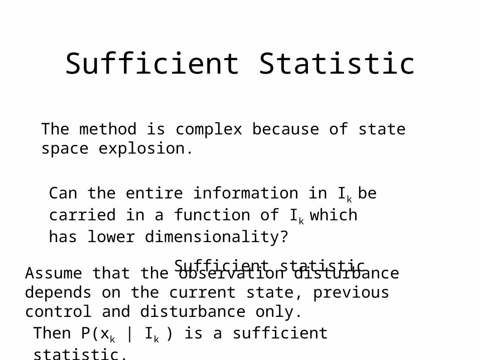
Sufficient Statistic
The method is complex because of state space explosion.
Can the entire information in Ik be carried in a function of Ik which has lower dimensionality?
Sufficient statistic
Assume that the observation disturbance depends on the current state, previous control and disturbance only.
Then P(xk | Ik ) is a sufficient statistic.
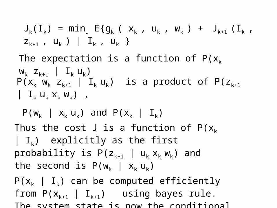
Jk(Ik) = minu E{gk ( xk , uk , wk ) + Jk+1 (Ik , zk+1 , uk ) | Ik , uk }
The expectation is a function of P(xk wk zk+1 | Ik uk)
P(xk wk zk+1 | Ik uk) is a product of P(zk+1 | Ik uk xk wk) ,
P(wk | xk uk) and P(xk | Ik)
Thus the cost J is a function of P(xk | Ik) explicitly as the first probability is P(zk+1 | uk xk wk) and the second is P(wk | xk uk)
P(xk | Ik) can be computed efficiently from P(xk+1 | Ik+1) using bayes rule. The system state is now the conditional probability distribution P(xk+1 | Ik+1)

Examples: Treasure searchingA site may contain a treasure.
If it contains the treasure, then the search yields the treasure with probability
The treasure is worth V units, each search costs C units, and the search has to terminate in N slots.
The state is the probability that the site contains the treasure given the previous controls and observations, pk
If we don’t search at a previous slot, we wouldn’t search in future.
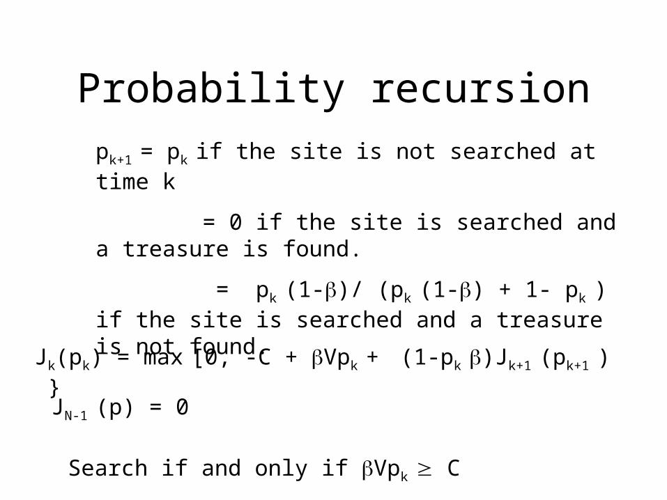
Probability recursion
pk+1 = pk if the site is not searched at time k
= 0 if the site is searched and a treasure is found.
= pk (1-)/ (pk (1-) + 1- pk ) if the site is searched and a treasure is not found.
Jk(pk) = max [0, -C + Vpk + (1-pk )Jk+1 (pk+1 ) }
JN-1 (p) = 0
Search if and only if Vpk C

General Form of the RecursionP(xk+1 | Ik+1) = P(xk+1 | Ik , uk, zk+1 )
= P(xk+1 zk+1 | Ik , uk)/ P(zk+1 | Ik , uk)
= P(xk+1 | Ik , uk) P(zk+1 | Ik , uk, xk+1 )/-
P(xk+1 | Ik , uk) P(zk+1 | Ik , uk, xk+1 ) dxk+1
xk+1 = fk (xk , uk , wk )
P(xk+1 | Ik , uk) = P(wk | Ik , uk)
= - P(xk | Ik ) P(wk | uk, xk ) dxk
P(zk+1 | Ik , uk xk+1 ) can be expressed in terms of P(vk+1 | xk , uk
wk ), P(wk | xk , uk ), P(xk | Ik )

Suboptimal Control
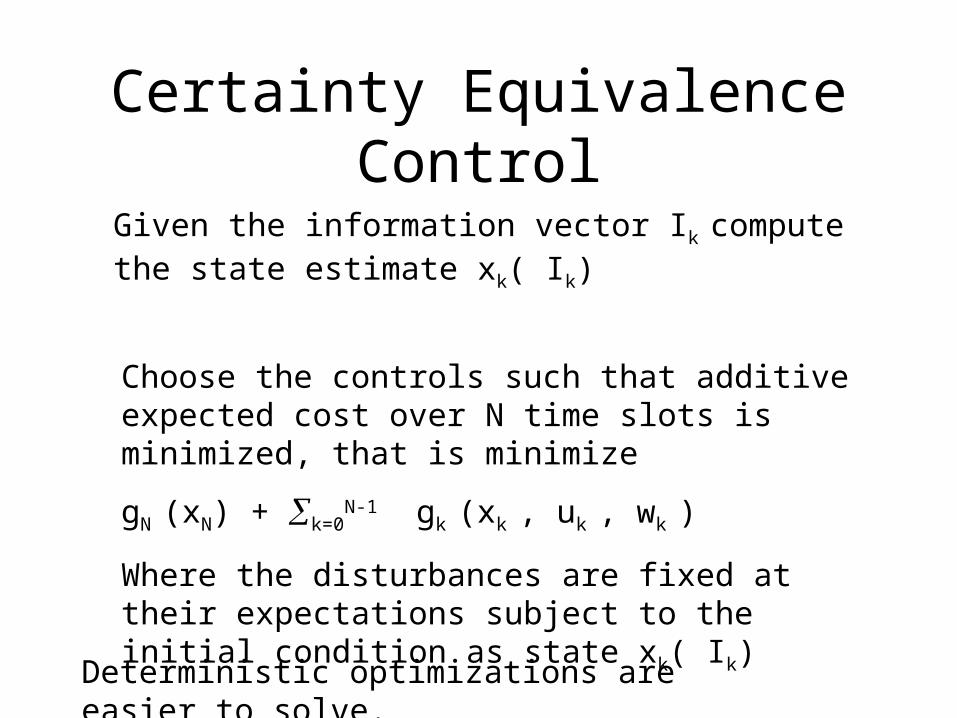
Certainty Equivalence Control
Given the information vector Ik compute the state estimate xk( Ik)
Choose the controls such that additive expected cost over N time slots is minimized, that is minimize
gN (xN) + k=0N-1 gk (xk , uk , wk )
Where the disturbances are fixed at their expectations subject to the initial condition as state xk( Ik)
Deterministic optimizations are easier to solve.
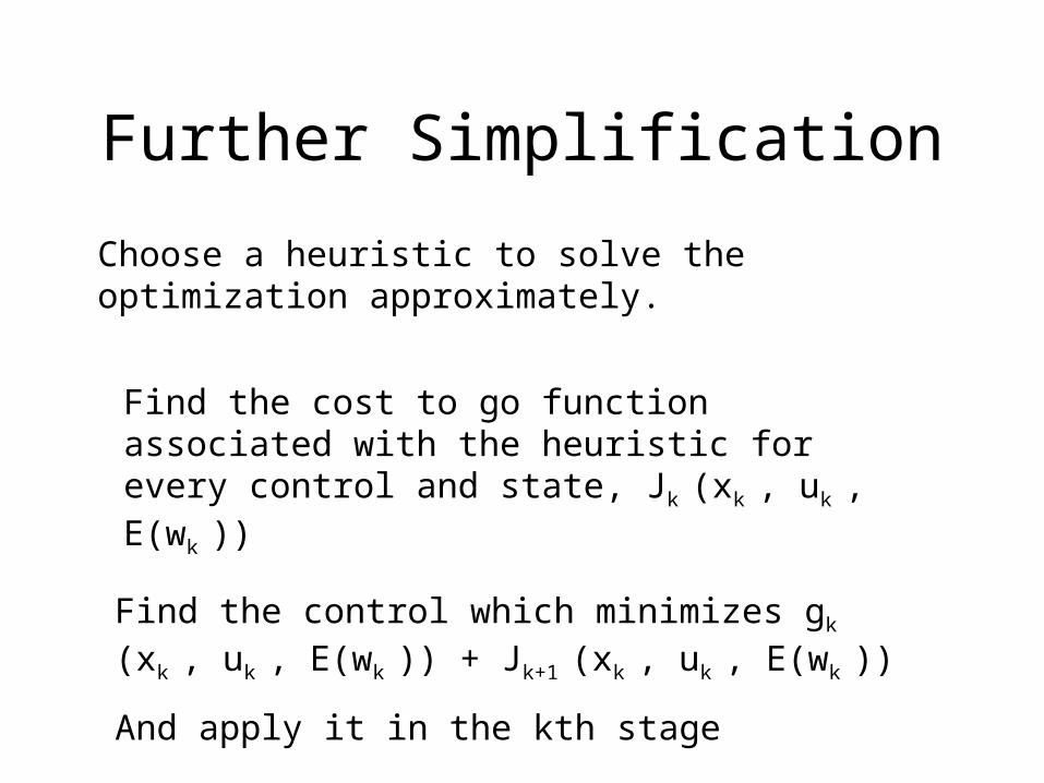
Further Simplification
Choose a heuristic to solve the optimization approximately.
Find the cost to go function associated with the heuristic for every control and state, Jk (xk , uk , E(wk ))
Find the control which minimizes gk (xk , uk , E(wk )) + Jk+1
(xk , uk , E(wk ))
And apply it in the kth stage

Partially stochastic certainty equivalence control
Applies for imperfect state information
Solve the DP assuming perfect state information
At every stage assume that the state is the expected value given the observation and the controls, and choose the controls accordingly.

Applications
Multiaccess communication
Hidden markov model

Open Loop Feedback Control
Similar to certainty equivalence controller, except that it uses the measurements to modify the distribution of expectation as well.
OLFC performs at least as well as the optimal open loop policy, but CEC does not provide such guarantee.

Limited Lookahead Policy
Find the control which minimizes E[gk (xk , uk , E(wk )) + Jk+1 (xk , uk , wk ))]
And apply it in the kth stage,
Where Jk+1 (xk , uk , wk ) is an approximation of the cost to go function.
One stage look ahead policy

Two stage lookahead policy
Approximate Jk+2 (xk , uk , wk )
Compute a two-stage DP with terminal cost Jk+2 (xk , uk , wk )
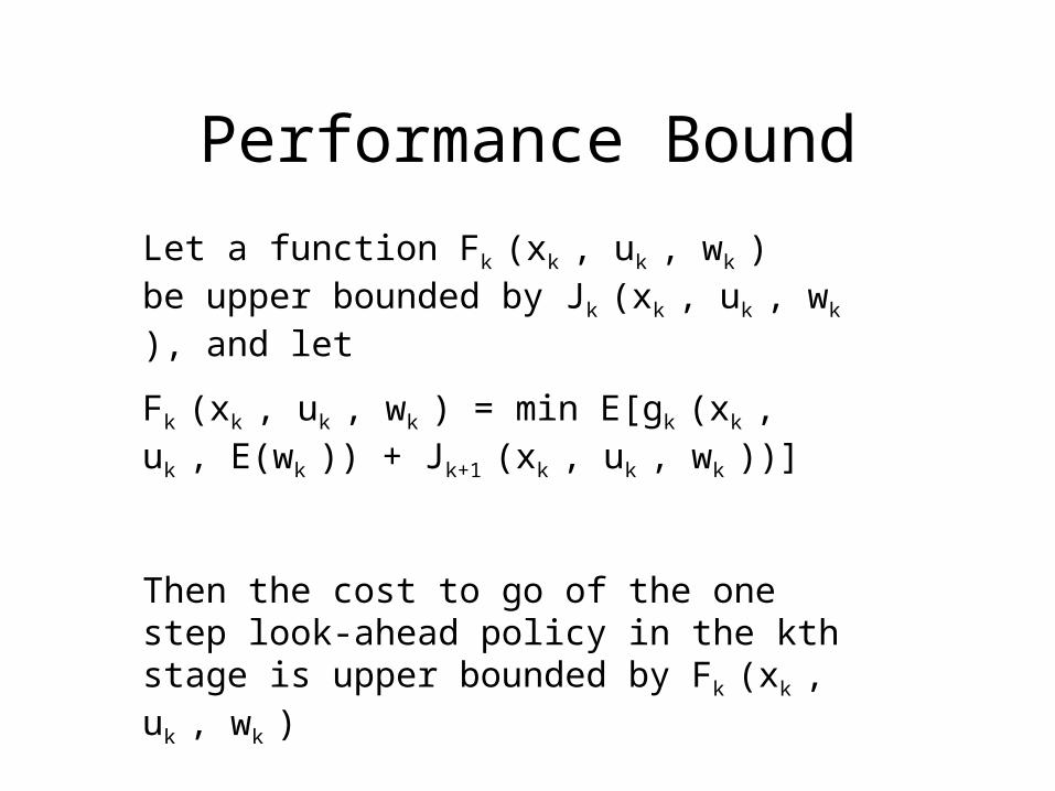
Performance Bound
Let a function Fk (xk , uk , wk ) be upper bounded by Jk (xk , uk , wk ), and let
Fk (xk , uk , wk ) = min E[gk (xk , uk , E(wk )) + Jk+1
(xk , uk , wk ))]
Then the cost to go of the one step look-ahead policy in the kth stage is upper bounded by Fk
(xk , uk , wk )

How to approximate?
Problem approximation
Use the cost to go of a related but simpler problem
Approximate the cost to go function by a parametrized function, and tune the parameters
Approximation architectures
Approximate the cost to go by that of a suboptimal strategy which is expected to be reasonably close.
Rollout policy
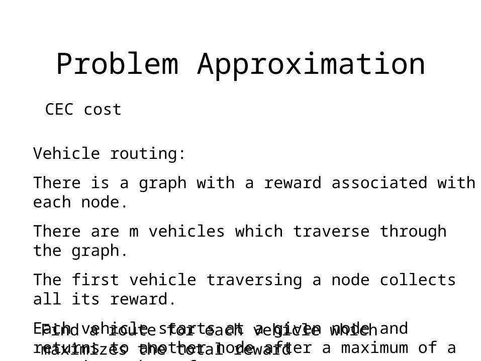
Problem Approximation
CEC cost
Vehicle routing:
There is a graph with a reward associated with each node.
There are m vehicles which traverse through the graph.
The first vehicle traversing a node collects all its reward.
Each vehicle starts at a given node and returns to another node after a maximum of a certain number of arcs.
Find a route for each vehicle which maximizes the total reward
Approximate cost to go is the optimal value to go of the following sub-optimal set of paths.
Fix the order of the vehicles
Obtain the path for each in order, reducing the rewards of the traversed nodes to 0 at all times.

Rollout policy
Sub-optimal policy to start with
Base policy
One step look-ahead always improves upon the base policy.

Example: Quiz Problem
A person is given a list of N questions.
Question j will be answered with probability pj
The person will receive a reward vj if he answers the jth question correctly.
The quiz terminates at the first incorrect answer.
The optimal ordering is to answer in decreasing order of pj vj /(1 - vj )
Variants where this solution can be used as a base
A limit on the maximum number of questions which can be answered.
A time window for each question where each question can be answered.
Precedence constraints

Infinite Horizon Problem

Problem Description
The objective is to maximize the total cost over an infinite horizon.
LimN Ek=0N-1 g (xk , uk , wk )
This limit need not exist!
Thus the objective is to minimize a discounted cost function where LimN Ek=0
N-1 k g (xk , uk , wk ) where discount factor is in (0, 1).
J(x) = LimN Ek=0N-1 k g (xk , uk , wk ) where
x0 = x

Classifications
Stochastic shortest path problem
Here the discount factor can be taken as 1
There is a termination state such that the system stays in the termination state once it reaches there.
The system reaches the termination state with probability 1
The horizon is in effect finite but its length is random.
Discounted problems
The cost per stage is bounded
Here the discount factor is less than 1
Absolute cost per stage is upper bounded
Thus LimN Ek=0N-1 k g (xk , uk , wk ) exists
The cost per stage is un-bounded
The analysis is more complicated

Average Cost Problem
Minimize LimN 1/NEk=0N-1 k g (xk , uk , wk )
Lim 0 (1- )J(0) is the average cost of the optimal strategy in many cases
Exists under certain special conditions.

Bellmans Equations
J(x) = minu in U(x) E { g(x, u, w ) + J (f(x,u,w)) }
The optimal costs J(x) satisfy Bellman’s equations
Given any initial condition, J0(x), the iteration
Jk+1(x) = minu in U(x) E { g(x, u, w ) + Jk (f(x,u,w)) }
Converges to the optimal discounted cost J(x)
(value iteration)
Optimal cost of any stationary policy
A policy is said to be stationary if it does not depend on the time index, that is given the control action in any slot j is same as that in any other slot k, if the state in both is the same
Optimal discounted cost of a stationary policy u can be found by solving the following equations:
J,u(x) = E { g(x, u(x), w ) + J ,u (f(x,u(x),w)) }
The solution can be obtained from the DP iteration, starting from any initial state
Jk+1(x) = E { g(x, u(x), w ) + Jk (f(x,u(x),w)) }
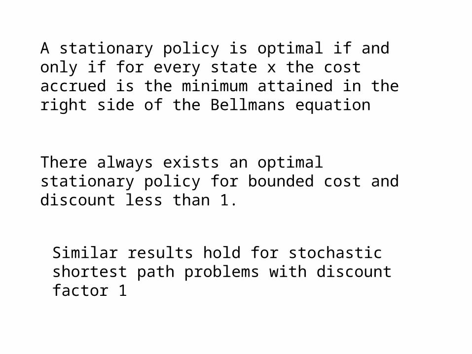
A stationary policy is optimal if and only if for every state x the cost accrued is the minimum attained in the right side of the Bellmans equation
There always exists an optimal stationary policy for bounded cost and discount less than 1.
Similar results hold for stochastic shortest path problems with discount factor 1
Stochastic Shortest Path
Battery management problem

Computational Strategies for solving Bellmans equations
Value iteration
Infinite number of iterations
Policy Iteration
Finite number of iterartions

Policy IterationStart from a stationary policy
Generate a sequence of new policies
Let the policy in the kth iteration be uk
Compute its cost by solving the following linear equations
J(x) = E { g(x, uk(x), w ) + J(f(x, uk(x), w)) }
The new policy uk+1 can be obtained using the solutions of the above, J(x), as follows:
uk+1(x) = arg minu in U(x) E { g(x, u(x), w ) + J (f(x,u(x),w)) }
The iteration stops when the current policy is the same as the previous policy.
The policy iteration terminates at the optimal policy in a finite number of iterations, and the cost of the policies are decreasing.
Continuous time MDP
Time is no longer slotted
State transitions occur at any time.
Markov: The system restarts itself at the instant of every transition.
Fresh control decisions taken at the instant of transitions.
Discretize the system by looking at the transition epochs only (these act like slot boundaries)
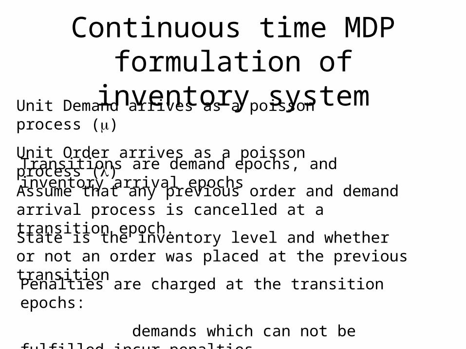
Continuous time MDP formulation of inventory system
Unit Demand arrives as a poisson process ()
Unit Order arrives as a poisson process ()
Transitions are demand epochs, and inventory arrival epochs
Assume that any previous order and demand arrival process is cancelled at a transition epoch.
State is the inventory level and whether or not an order was placed at the previous transition
Penalties are charged at the transition epochs:
demands which can not be fulfilled incur penalties
orders are charged at delivery
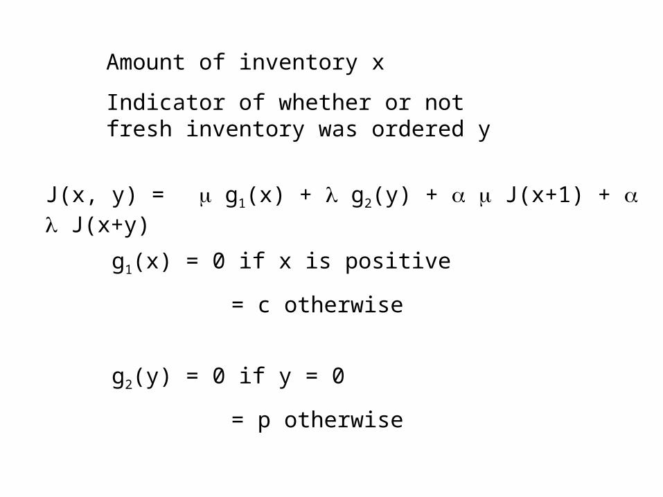
J(x, y) = g1(x) + g2(y) + J(x+1) + J(x+y)
Amount of inventory x
Indicator of whether or not fresh inventory was ordered y
g1(x) = 0 if x is positive
= c otherwise
g2(y) = 0 if y = 0
= p otherwise
![[Bertsekas D., Tsitsiklis J.] Parallel and Distrib(Book4You)](https://static.documents.pub/doc/80x56/577c83471a28abe054b456ef/bertsekas-d-tsitsiklis-j-parallel-and-distribbook4you.jpg)


![[Bertsekas D., Tsitsiklis J.] Parallel and org](https://static.documents.pub/doc/80x56/577d208b1a28ab4e1e932bcc/bertsekas-d-tsitsiklis-j-parallel-and-org.jpg)


