1

Background Report: An Overview of the OECD ENV-Linkages model

By Jean-Marc Burniaux and Jean Chateau, OECD

May 2010

Background report to the joint report by IEA, OPEC, OECD and World Bank on “Analysis of

the Scope of Energy Subsidies and Suggestions for the G-20 Initiative”

2

The OECD ENV-Linkages General Equilibrium model is the successor to the OECD GREEN model

for environmental studies, which was initially developed by the OECD Economics Department (Burniaux,

et al. 1992) and is now hosted at the OECD Environment Directorate. GREEN was originally used for

studying climate change mitigation policy and culminated in Burniaux (2000). Previous works using

extensively the model include two books : OECD (2008) and OECD(2009). Exploration of some of the

model’s properties and some sensitivity analysis is reported in OECD (2006).

1. The structure of the model

Key features

The ENV-Linkages model is a recursive dynamic neo-classical general equilibrium model. It is a

global economic model built primarily on a database of national economies. In the version of the model

used here, the world economy is divided in 12 countries/regions, each with 25 economic sectors (Tables 1

and 2), including five different technologies to produce electricity. Each of the 12 regions is underpinned

by an economic input-output table (usually sourced from national statistical agencies). The database has

been built and maintained at Purdue University by the Global Trade Analysis Project (GTAP) consortium.

A fuller description of the database can be found at Dimaranan (2006). Those tables identify all the inputs

that go into an industry, and identify all the industries that buy specific products.

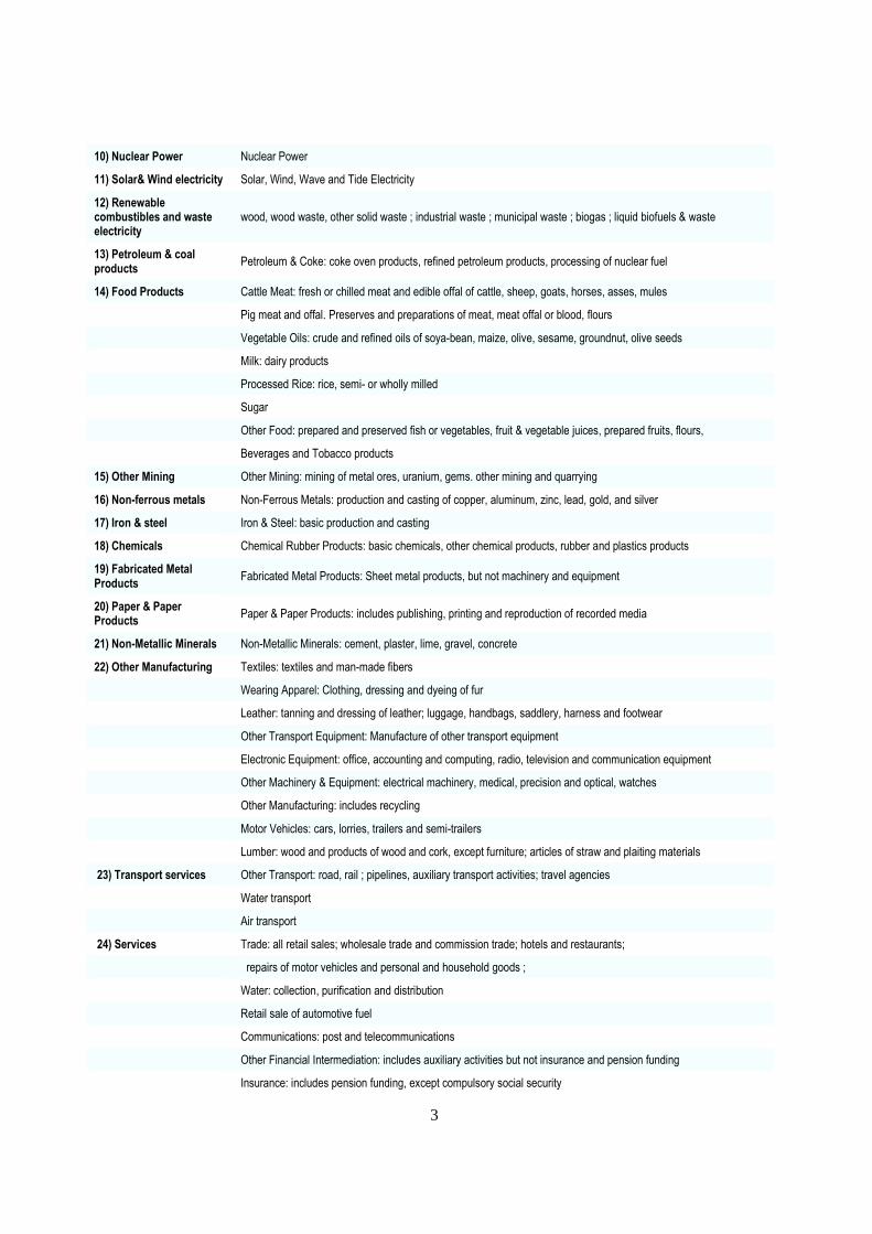
Table 1. ENV-Linkages model sectors

Labels Description

1) Rice Paddy rice: rice, husked and in the husk.

2) Other crops Wheat: wheat and meslin

Other Grains: maize (corn), barley, rye, oats, other cereals

Veg & Fruit: vegetables, fruits, fruit and nuts, potatoes, cassava, truffles.

Oil Seeds: oil seeds and oleaginous fruits; soy beans, copra

Cane & Beet: sugar cane and sugar beet

Plant fibers: cotton, flax, hemp, sisal and other raw vegetable materials used in textiles

Other Crops

3) Livestock Cattle: cattle, sheep, goats, horses, asses, mules, and hinnies; and semen thereof

Other Animal Products: swine, poultry and other live animals; eggs, in shell, natural honey, snails

Raw milk

Wool: wool, silk, and other raw animal materials used in textile

4) Forestry Forestry: forestry, logging and related service activities

5) Fisheries Fishing: hunting, trapping and game propagation including related service activities, fishing,

fish farms; service activities incidental to fishing

6) Crude Oil Parts of extraction of crude petroleum & service activities incidental to oil extraction excl. surveying

7) Gas extraction and distribution

Pars of extraction of natural gas & service activities incidental to gas extraction excl. surveying

distribution of gaseous fuels through mains; steam and hot water supply

8) Fossil Fuel Based Electricity

Coal, Coal gases, Natural gases and oil fired electricity (production, collection and distribution)

9) Hydro and Geothermal electricity

Hydroelectric power and Geothermal electricity

3

10) Nuclear Power Nuclear Power

11) Solar& Wind electricity Solar, Wind, Wave and Tide Electricity

12) Renewable combustibles and waste electricity

wood, wood waste, other solid waste ; industrial waste ; municipal waste ; biogas ; liquid biofuels & waste

13) Petroleum & coal products

Petroleum & Coke: coke oven products, refined petroleum products, processing of nuclear fuel

14) Food Products Cattle Meat: fresh or chilled meat and edible offal of cattle, sheep, goats, horses, asses, mules

Pig meat and offal. Preserves and preparations of meat, meat offal or blood, flours

Vegetable Oils: crude and refined oils of soya-bean, maize, olive, sesame, groundnut, olive seeds

Milk: dairy products

Processed Rice: rice, semi- or wholly milled

Sugar

Other Food: prepared and preserved fish or vegetables, fruit & vegetable juices, prepared fruits, flours,

Beverages and Tobacco products

15) Other Mining Other Mining: mining of metal ores, uranium, gems. other mining and quarrying

16) Non-ferrous metals Non-Ferrous Metals: production and casting of copper, aluminum, zinc, lead, gold, and silver

17) Iron & steel Iron & Steel: basic production and casting

18) Chemicals Chemical Rubber Products: basic chemicals, other chemical products, rubber and plastics products

19) Fabricated Metal Products

Fabricated Metal Products: Sheet metal products, but not machinery and equipment

20) Paper & Paper Products

Paper & Paper Products: includes publishing, printing and reproduction of recorded media

21) Non-Metallic Minerals Non-Metallic Minerals: cement, plaster, lime, gravel, concrete

22) Other Manufacturing Textiles: textiles and man-made fibers

Wearing Apparel: Clothing, dressing and dyeing of fur

Leather: tanning and dressing of leather; luggage, handbags, saddlery, harness and footwear

Other Transport Equipment: Manufacture of other transport equipment

Electronic Equipment: office, accounting and computing, radio, television and communication equipment

Other Machinery & Equipment: electrical machinery, medical, precision and optical, watches

Other Manufacturing: includes recycling

Motor Vehicles: cars, lorries, trailers and semi-trailers

Lumber: wood and products of wood and cork, except furniture; articles of straw and plaiting materials

23) Transport services Other Transport: road, rail ; pipelines, auxiliary transport activities; travel agencies

Water transport

Air transport

24) Services Trade: all retail sales; wholesale trade and commission trade; hotels and restaurants;

repairs of motor vehicles and personal and household goods ;

Water: collection, purification and distribution

Retail sale of automotive fuel

Communications: post and telecommunications

Other Financial Intermediation: includes auxiliary activities but not insurance and pension funding

Insurance: includes pension funding, except compulsory social security

4

Other Business Services: real estate, renting and business activities

Recreation & Other Services: recreational, cultural and sporting activities, other service activities;

private households with employed persons

Other Services (Government): public administration and defense; compulsory social security,

education, health and social work, sewage and refuse disposal, sanitation and similar activities,

activities of membership organizations n.e.c., extra-territorial organizations and bodies

25) Construction & Dwellings

Construction: building houses factories offices and roads

Dwellings: ownership of dwellings (imputed rents of houses occupied by owners)

Table 2. ENV-Linkages model regions

ENV-Linkages regions GTAP countries/regions

1) Australia, New Zealand Australia, New Zealand

2) Japan Japan

3) Canada Canada

4) United States United States

5) European Union and EFTA Austria, Belgium, Denmark, Finland, Greece, Ireland, Luxembourg, Netherlands, Portugal, Sweden, France, Germany, United Kingdom, Italy, Spain, Switzerland, Rest of EFTA, Czech Republic, Slovakia, Hungary, Poland, Romania, Bulgaria, Cyprus, Malta, Slovenia, Estonia, Latvia, Lithuania

6) Brazil Brazil

7) China China, Hong Kong

8) India India

9) Russia Russian Federation

10) Oil producing countries Indonesia, Venezuela, Rest of Middle East, Islamic Republic of Iran, Rest of North Africa, Nigeria

11) Rest of Annex 1 countries Croatia, Rest of Former Soviet Union

12) Rest of the world

Korea, Taiwan, Malaysia, Philippines, Singapore, Thailand, Viet Nam, Rest of East Asia, Rest of Southeast Asia, Cambodia, Rest of Oceania, Bangladesh, Sri Lanka, Rest of South Asia, Pakistan, Mexico, Rest of North America, Central America, Rest of Free Trade Area of Americas, Rest of the Caribbean, Colombia, Peru, Bolivia, Ecuador, Argentina, Chile, Uruguay, Rest of South America, Paraguay, Turkey, Rest of Europe, Albania, Morocco, Tunisia, Egypt, Botswana, Rest of South African Customs Union, Malawi, Mozambique, Tanzania, Zambia, Zimbabwe, Rest of Southern African Development Community, Mauritius, Madagascar, Uganda, Rest of Sub-Saharan Africa, Senegal, South Africa.

5

Production

All production in ENV-Linkages is assumed to operate under cost minimisation with an assumption

of perfect markets and constant return to scale technology. The production technology is specified as

nested CES production functions in a branching hierarchy. Figure 1 illustrates the typical nesting of the

model’s sectors (some sectors, like agriculture have a different nesting). The nesting of the electricity

production is slightly different and is reported in Figure 2. In Figure 1 and 2, each node represents a

constant elasticity of substitution (CES) production function. This gives marginal costs and represents the

different substitution (and complementarity) relations across the various inputs in each sector. Each sector

uses intermediate inputs – including energy inputs - and primary factors (labour and capital). In some sectors,

primary factors include natural resources, e.g. trees in forestry, land in agriculture, etc.

In a way similar to Hyman et al. (2002), the top-level production nest considers final output as a composite

commodity combining emissions of non-CO2 gases and the production of the sector net of these emissions.

In sectors that do not emit non-CO2 gases, the corresponding emission rate is set equal to zero. For the

purpose of calibration, these non-CO2 gases are valuated using an arbitrary very low carbon price. The

following non-CO2 emission sources are considered: i) methane from rice cultivation, livestock production

(enteric fermentation and manure management), coal mining, crude oil extraction, natural gas and services

(landfills); ii) nitrous oxide from crops (nitrogenous fertilizers), livestock (manure management),

chemicals (non-combustion industrial processes) and services (landfills); iii) industrial gases (SF6, PFC’s

and HFC’s) from chemicals industry (foams, adipic acid, solvents), aluminum, magnesium and semi-

conductors production. The values of the substitution elasticities are calibrated such as to fit to marginal

abatement curves available in the literature on alternative technology options (US-EPA, 2006b).

The second-level nest considers the gross output of sector (net of GHGs) as a combination of aggregate

intermediate demands and a value-added bundle, including energy. For each good or service, output is

produced by different production streams which are differentiated by capital vintage (old and new). Capital

that is implemented contemporaneously is new – thus investment impacts on current-period capital; but

then becomes old capital (added to the existing stock) in the subsequent period. Each production stream

has an identical production structure, but with different technological parameters and substitution

elasticities. Letting Xi,v represents gross output of sector i (net of GHGs) using capital of vintage v, the

equations representing production are derived from first order conditions [1]-[3] of the firm’s profit

maximisation objective.

vi

vINT

i

vi

vi

INT

vii XP

VCAINT

pvi

pvi

,

,1

,,

,

,

[1]

viVA

i

vi

vi

VA

vivi XP

VCAVA

pvi

pvi

,

,1

,,,

,

,

[2]

))1/(1(

1

,

1

,,

,,,1

pvip

vipvi VA

i

VA

vi

INT

i

INT

vi

i

vi PPA

VC

[3]

where INT is the intermediate demand bundle (PINT

its price), VA represents value-added (PVA

its price), VC

is unit variable cost of producing one unit of net of GHGs output (average costs include the cost of capital),

A is a technical change term. In order to determine the industry-wide cost that includes both capital

vintages, there is an averaging (weighted) of variable costs across the two vintages.

6

Figure 1. Structure of production in ENV-Linkages

Note: see Table 3 for parameter values

In each period, the supply of primary factors (e.g. capital, labour, land and natural resources) is usually

predetermined. On the right hand side of the tree in Figure 1 value-added1 is shown as being composed of a

labour input [4] along with a composite capital/energy bundle [5]:

vi

i

VA

vi

i

v

L

vii VAW

PL

Vvi

Vvi

,

,1

,

,

,

[4]

1 The valued-added bundle is specified as a CES combination of labour and a broad concept of capital. In the ―crop‖

production sector, this capital is itself a CES combination of fertilizer and another bundle of capital-land-energy. The

intention of this specification is to reflect the possibility of substitution between intensive and extensive agriculture.

In the ―livestock‖ sector, substitution possibilities are between bundles of land and feed, on the one hand, reflecting a

similar choice between extensive and intensive livestock production, and of capital-energy-labour bundle, on the

other hand.

Non – CO2 GHG

Domestic goods and services

Demand for Intermediate goods and services

Demand for Labour

Value-added plus energy

Imported goods and services

Demand for Capital and Energy

Substitution between material inputs and VA plus energy (σp)

«Armington» specification (σm)

Substitution between material inputs (σn)

Demand for Energy (fig 2)

Demand for Capital and Specific factor

Capital Specific factor Demand by region of origin

Substitution between VA and Energy (σv)

Substitution between Capital and Specific Factor (σE)

Substitution between Capital and Specific Factor (σ

k)

Gross Output of sector i

Net-of-GHG Output Non-CO2 GHG Bundle

Substitution between GHGs Bundle and output (σGhg

)

Sub. between GHG (σemi

)

7

viKE

vi

VA

viKE

vivi VAP

PKE

Vvi

,

,

,

,,

,

[5]

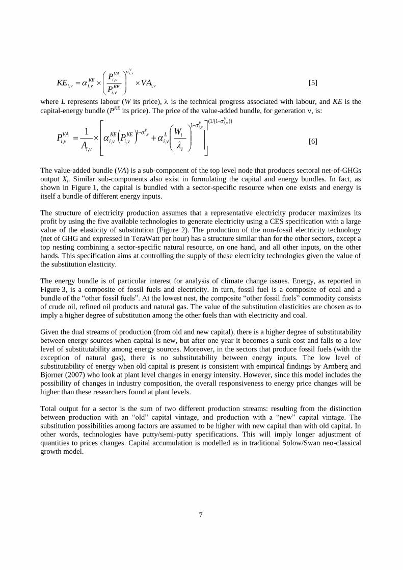
where L represents labour (W its price), is the technical progress associated with labour, and KE is the

capital-energy bundle (PKE

its price). The price of the value-added bundle, for generation , is:

))1/(1(

1

,

1

,,

,

,

,,

,1

VviV

viV

vi

i

iL

vi

KE

vi

KE

vi

vi

VA

vi

WP

AP

[6]

The value-added bundle (VA) is a sub-component of the top level node that produces sectoral net-of-GHGs

output Xi. Similar sub-components also exist in formulating the capital and energy bundles. In fact, as

shown in Figure 1, the capital is bundled with a sector-specific resource when one exists and energy is

itself a bundle of different energy inputs.

The structure of electricity production assumes that a representative electricity producer maximizes its

profit by using the five available technologies to generate electricity using a CES specification with a large

value of the elasticity of substitution (Figure 2). The production of the non-fossil electricity technology

(net of GHG and expressed in TeraWatt per hour) has a structure similar than for the other sectors, except a

top nesting combining a sector-specific natural resource, on one hand, and all other inputs, on the other

hands. This specification aims at controlling the supply of these electricity technologies given the value of

the substitution elasticity.

The energy bundle is of particular interest for analysis of climate change issues. Energy, as reported in

Figure 3, is a composite of fossil fuels and electricity. In turn, fossil fuel is a composite of coal and a

bundle of the ―other fossil fuels‖. At the lowest nest, the composite ―other fossil fuels‖ commodity consists

of crude oil, refined oil products and natural gas. The value of the substitution elasticities are chosen as to

imply a higher degree of substitution among the other fuels than with electricity and coal.

Given the dual streams of production (from old and new capital), there is a higher degree of substitutability

between energy sources when capital is new, but after one year it becomes a sunk cost and falls to a low

level of substitutability among energy sources. Moreover, in the sectors that produce fossil fuels (with the

exception of natural gas), there is no substitutability between energy inputs. The low level of

substitutability of energy when old capital is present is consistent with empirical findings by Arnberg and

Bjorner (2007) who look at plant level changes in energy intensity. However, since this model includes the

possibility of changes in industry composition, the overall responsiveness to energy price changes will be

higher than these researchers found at plant levels.

Total output for a sector is the sum of two different production streams: resulting from the distinction

between production with an ―old‖ capital vintage, and production with a ―new‖ capital vintage. The

substitution possibilities among factors are assumed to be higher with new capital than with old capital. In

other words, technologies have putty/semi-putty specifications. This will imply longer adjustment of

quantities to prices changes. Capital accumulation is modelled as in traditional Solow/Swan neo-classical

growth model.

8

Figure 2. Structure of electricity generation

Structure of production of non-fossil technologies

Gross output of Electricity

Substitution between Electricity technology (σelec

)

))

Nuclear Hydro Wind & Solar RENEW Fossil-fuelled (see. Fig. 1)

See Fig. below for these technologies

Domestic goods and services

Demand for intermediate goods and services incl. electricity

Demand for Labour

Value-added

Imported goods and services

Demand for Capital

Substitution between material inputs and VA (σp)

« Armington » specification

Substitution between material inputs (σn)

Demand by region of origin

Substitution between VA and Energy (σv)

Net of GHG output in Twh

Net-of-Natural Resource Output Natural Resource

Substitution between Natural Resource and other inputs (σnatr

)

))

9

Figure 3. Structure of energy intermediate demands Figure 2. Structure of energy demand in ENV-Linkages

Note: See Table 1 for parameter value.

Source: OECD.

TOTAL ENERGY DEMAND

Electricity Fossil fuels

CoalOther fossil

fuels

Crude oil Refined oil products

Natural gas

Consumption

Household consumption demand is the result of static maximization behaviour which is formally

implemented as an ―Extended Linear Expenditure System‖. A representative consumer in each region –

who takes prices as given – optimally allocates disposal income among the full set of consumption

commodities and savings. Saving is considered as a standard good and therefore does not rely on a

forward-looking behaviour by the consumer. Formally, a representative consumer maximises well-being

(utility) subject to resource constraints:

1,

)ln()ln(

s

k

k

k

k

c

k

s

skk

k

k

andYSCPtoSubject

P

SCUMax

where U represents utility, C is a vector of k consumer goods, Pc is the vector of consumer prices, S

represents the value of saving, Ps the relevant price of saving, and Y is total net-of-taxes income

(completely allocated between consumption and savings). The parameter θ is the floor level of

consumption – its main function is in making the utility function non-homothetic, which is consistent with

considerable empirical evidence (e.g. Dowrick, et al. 2003). Since consumers are not represented with

forward-looking behavior, some care needs to be exercised in studying policies that consumers may

reasonably be expected to anticipate – either the policy itself or its consequences. For each country, the

consumer’s objective function thus gives rise to household private consumptions [7] and saving [8]:

k

k

c

k

c

c

k

k

kk PPopYYwhereYP

PopC

** , [7]

10

k

k

c

k

c CPYS [8]

where Pop represents population, Yc represents household disposable income and Y* is a supernumerary

income (i.e. income above the subsistence level).

Foreign Trade

World trade is based on a set of regional bilateral flows. The basic assumption is that imports

originating from different regions are imperfect substitutes Therefore in each region, total import demand

for each good is allocated across trading partners according to the relationship between their export prices.

This specification of imports - commonly referred to as the Armington specification - formally implies that

each region faces a reduction in demand for its exports if domestic prices increase. The Armington

specification is implemented using two CES nests. At the top nest, domestic agents choose the optimal

combination of the domestic good and an aggregate import good[9]. At the second nest, agents optimally

allocate demand for the aggregate import good [11] across the range of trading partners r’.

i

i

im

ii XAPMT

PAXMT

mi

[9]

))1/(1(1

,,

,

wi

wri

ri

r

W

rii PMPMT

[10]

where XMT is the bundle of imports of a particular good or service (PMT its price) and XA represents the

aggregate demand for domestically produced and import goods (PA is its price).

iM

ir

iw

irir XMTPM

PMTWTF

wi

,'

,',' [11]

where WTFr' is import of a particular good or service from region r'. Its price, PMr', represents the domestic

import price (e.g. domestic producer price of its partner r’ adjusted for export tax or subsidy, transport

margin, ―iceberg‖ costs, and domestic tariffs).

Investment and Market goods equilibria

This version of the model does not include an investment schedule that relates investment to

interest rates. In each period, investment net-of-economic depreciation is equal to the sum of government

savings, consumer savings and net capital flows from abroad. Investment as well as government demand

use final goods according with a CES specification. Then, the total demand of a good in the economy is

equal to the consumer final demand plus the intermediary demands from firms plus the intermediary

demands by final good sectors, corresponding to government and investment expenditures.

Market goods equilibria imply that, on the one side, the total production of any good or service is equal to

the demand addressed to domestic producers plus exports; and, on the other side, the total demand is

allocated, according to the Armington principle, between the demands (both final and intermediary)

addressed to domestic producers and the import demand(see below).

Government and long-term closure

Government collects income taxes, indirect taxes on intermediate and final consumption as well as

possible carbon taxes, production taxes, tariffs, and export taxes/subsidies. Aggregate government

expenditures are linked to real GDP. Since predicting corrective government policy is not an easy task, the

11

real government deficit is exogenous. The closure of the model implies that some fiscal instrument is

endogenous – in order to meet government budget constraint. Given also a sequence of public savings (or

deficits), the fiscal closure rule in ENV-Linkages is that the income tax rate adjusts to offset changes that

may arise in government expenditures, or as a result of other taxes. For example, an elimination of subsidies

rates is compensated by a decrease in household direct taxation or an increase in transfert to household for non

OECD countries, ceteris paribus. Alternative closure rules can be easily implemented.

For studying the impacts of climate change policy, four types of instruments have been developed: GHG

taxes, global or specific by sectors, gases or emission sources; tradable emission permits (with flexibility

between regions and sectors); offsets (including the Clean Development Mechanism) and regulatory policy

(modelled as quantity constraints). Taxes and tradable permits are applied on inputs of fossil-fuel

producing sectors (refined petroleum, natural gas, coal). They are applied, as well, on final demands of

fossil-based energy. Regulatory policy has also been introduced in the model through a mechanism

imposing a shadow cost on the firm’s inputs or capital. It has the effect of changing the marginal cost of

particular inputs, or changing the quantity of capital used to produce a given output, but does use market

instruments. The analysis requires assumptions concerning the cost of the regulatory policy, but it breaks

the link between policy instruments and revenue transfer that is inherent in tax policy and tradable permits

(Burniaux, et al. 2008).

Factor-income taxes as well as factor taxes and subsidies on factor supply have also been introduced as

these instruments are distinguished in the GTAP version 6.2 database. From IEA(2010) databases we

have also introduced fossil-fuel subsidies to energy demands.

Each region runs a current-account surplus (or deficit), which is fixed (in terms of the model numéraire).

Closure on the international side of each economy is achieved by having, as a counterpart of these

imbalances, a net outflow (or inflow) of capital, which is subtracted from (added to) the domestic flow of

saving. These net capital flows are exogenous. In each period, the model equates investment to saving (which is

equal to the sum of saving by households, the net budget position of the government and foreign capital

flows). Hence, given exogenous sequences for government and foreign savings, this implies that investment

is ultimately driven by household savings.

ENV-Linkages is fully homogeneous in prices and only relative prices matter. All prices are expressed

relatively to the numéraire of the price system that is arbitrarily chosen as the index of OECD

manufacturing exports prices. From the point of view of the model specification, this has an impact on the

evaluation of international investment flows. They are evaluated with respect to the price of the numéraire

good. Therefore, one way to interpret the foreign investment flows is as the quantity of foreign saving

which will buy the average bundle of OECD manufacturing exports.

Dynamic Features

The ENV-Linkages model has a simple recursive dynamic structure as agents are assumed to be myopic and

to base their decisions on static expectations concerning prices and quantities. Dynamics in the model

originate from two endogenous sources: i) accumulation of productive capital and ii) the putty/semi-putty

specification of technology, as well as, from exogenous drivers like population growth or productivity

changes.

At an aggregate level, the basic capital accumulation function equates the current capital stock to the

depreciated stock inherited from the previous period plus investment. Differences in sectoral rates of return

determine the allocation of investment across sectors. The model features two vintages of capital, but

investment adds only to new capital. Sectors with higher investment, therefore, are more able to adapt to

12

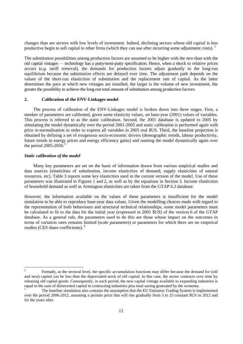
changes than are sectors with low levels of investment. Indeed, declining sectors whose old capital is less

productive begin to sell capital to other firms (which they can use after incurring some adjustment costs). 2

The substitution possibilities among production factors are assumed to be higher with the new than with the

old capital vintages — technology has a putty/semi-putty specification. Hence, when a shock to relative prices

occurs (e.g. tariff removal), the demands for production factors adjust gradually to the long-run

equilibrium because the substitution effects are delayed over time. The adjustment path depends on the

values of the short-run elasticities of substitution and the replacement rate of capital. As the latter

determines the pace at which new vintages are installed, the larger is the volume of new investment, the

greater the possibility to achieve the long-run total amount of substitution among production factors.

2. Calibration of the ENV-Linkages model

The process of calibration of the ENV-Linkages model is broken down into three stages. First, a

number of parameters are calibrated, given some elasticity values, on base-year (2001) values of variables.

This process is referred to as the static calibration. Second, the 2001 database is updated to 2005 by

simulating the model dynamically over the period 2001-2005 and static calibration is performed again with

price re-normalisation in order to express all variables in 2005 real $US. Third, the baseline projection is

obtained by defining a set of exogenous socio-economic drivers (demographic trends, labour productivity,

future trends in energy prices and energy efficiency gains) and running the model dynamically again over

the period 2005-2050.3

Static calibration of the model

Many key parameters are set on the basis of information drawn from various empirical studies and

data sources (elasticities of substitution, income elasticities of demand, supply elasticities of natural

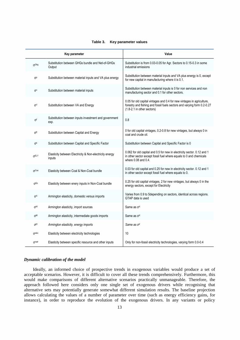
resources, etc). Table 3 reports some key elasticities used in the current version of the model. Use of these

parameters was illustrated in Figures 1 and 2, as well as by the equations in Section 3. Income elasticities

of household demand as well as Armington elasticities are taken from the GTAP 6.2 database.

However, the information available on the values of these parameters is insufficient for the model

simulation to be able to reproduce base-year data values. Given the modelling choices made with regard to

the representation of both behaviours and structural technical relationships, some model parameters must

be calculated to fit to the data for the initial year (expressed in 2001 $US) of the version 6 of the GTAP

database. As a general rule, the parameters used to do this are those whose impact on the outcomes in

terms of variation rates remains limited (scale parameters) or parameters for which there are no empirical

studies (CES share coefficients). 4

2 Formally, at the sectoral level, the specific accumulation functions may differ because the demand for (old

and new) capital can be less than the depreciated stock of old capital. In this case, the sector contracts over time by

releasing old capital goods. Consequently, in each period, the new capital vintage available to expanding industries is

equal to the sum of disinvested capital in contracting industries plus total saving generated by the economy. 3 The baseline simulation also contains the assumption that the EU Emission Trading System is implemented

over the period 2006-2012, assuming a permits price that will rise gradually from 5 to 25 constant $US in 2012 and

for the years after.

13

Table 3. Key parameter values

Key parameter Value

σGhg Substitution between GHGs bundle and Net-of-GHGs Output

Substitution is from 0.03-0.05 for Agr. Sectors to 0.15-0.3 in some industrial emissions

σp Substitution between material inputs and VA plus energy Substitution between material inputs and VA plus energy is 0, except for new capital in manufacturing where it is 0.1.

σn Substitution between material inputs Substitution between material inputs is 0 for non services and non manufacturing sector and 0.1 for other sectors.

σV Substitution between VA and Energy 0.05 for old capital vintages and 0.4 for new vintages in agriculture, forestry and fishing and fossil fuels sectors and varying form 0.2-0.27 (1.8-2.1 in other sectors)

σf Substitution between inputs investment and government exp.

0.8

σE Substitution between Capital and Energy 0 for old capital vintages, 0.2-0.8 for new vintages, but always 0 in coal and crude oil.

σk Substitution between Capital and Specific Factor Substitution between Capital and Specific Factor is 0

σELY Elasticity between Electricity & Non-electricity energy inputs

0.062 for old capital and 0.5 for new in electricity sector. 0.12 and 1 in other sector except fossil fuel where equals to 0 and chemicals where 0.08 and 0.4.

σCoa Elasticity between Coal & Non-Coal bundle 0.03 for old capital and 0.25 for new in electricity sector. 0.12 and 1 in other sector except fossil fuel where equals to 0.

σEp Elasticity between enery inputs in Non-Coal bundle 0.25 for old capital vintages, 2 for new vintages, but always 0 in the energy sectors, except for Electricity

σX Armington elasticity, domestic versus imports Varies from 0.9 to 5depending on sectors, identical across regions. GTAP data is used

σW Armington elasticity, import sources Same as σX

σM Armington elasticity, intermediate goods imports Same as σX

σEI Armington elasticity, energy imports Same as σX

σelec Elasticity between electricity technologies 10

σnatr Elasticity between specific resource and other inputs Only for non-fossil electricity technologies, varying form 0.0-0.4

Dynamic calibration of the model

Ideally, an informed choice of prospective trends in exogenous variables would produce a set of

acceptable scenarios. However, it is difficult to cover all these trends comprehensively. Furthermore, this

would make comparisons of different alternative scenarios practically unmanageable. Therefore, the

approach followed here considers only one single set of exogenous drivers while recognising that

alternative sets may potentially generate somewhat different simulation results. The baseline projection

allows calculating the values of a number of parameter over time (such as energy efficiency gains, for

instance), in order to reproduce the evolution of the exogenous drivers. In any variants or policy

14

simulations, these parameter values are kept constant while all other variables in the model are fully

endogenous.5

The list of exogenous drivers specified in the baseline projection is the following:

Demographic projections and employment trends,

Aggregate average and sectoral labour productivity growth, controlled by calibration of

technical progress coefficients embodied in labour,

Autonomous efficiency gains for capital, land and specific natural resources,

Autonomous efficiency gains of fertilizers in crops sectors and of the food bundle in livestock

rearing,

Supply of land and natural resources (excepted for fossil fuels sectors),

International trade margins,

Shares of public expenditure in real GDP,

Public savings and flows of international savings,

Energy demands (projected by using elasticities of demands to GDP), for all kind of fuels

demands excepted crude oil, controlled by calibration of the Autonomous Energy Efficiency

Improvements (named AEEIs) in energy use, by sector and type of fuel,

International prices of fossil fuels, controlled by calibration of the potential supply of fossil

fuels resources,

Investment to GDP ratios, controlled by calibration of the marginal propensity to save of the

households,

Non-CO2 fuel GHGs emissions, controlled by calibration of autonomous efficiency gains in

non-CO2 GHGs emissions, by sector and type of GHGs emissions,

The share of each type of electricity-producing technology, controlled by calibration of the

specific ―natural resource‖.

Note on data sources

Socio-economic variables like apparent labour productivity, investment to GDP ratios and employment

rate are taken from Duval, R. and C. De la Maisonneuve (2010) while population data are from UN(2006).

Sectoral labour productivity growth rates used to calibrated the model are extracted from OECD-STAN

database as well as Groningen Database for non-OECD countries. The mixing of these assumptions imply

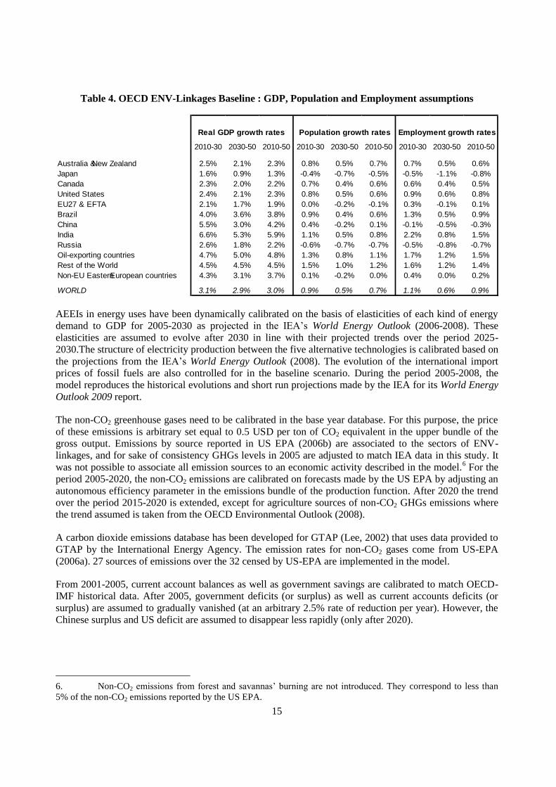
GDP growth rates as projected in Table 4.

GDP projections are based on convergence assumptions about labour productivity but other socio-

economic factors explain differences across countries. For example, while China and India labour

productivity growths are exactly the same over the period 2010-2050 (around 4.4% by year), India GDP is

projected to grow much faster than in China .This reflects that active population should still growing at a

important rythm in India while it is declining in China.

5 For instance, in the baseline scenario, the technical progress embodied in labour is calibrated to reproduce

given GDP trends. In contrast, in any policy variants, GDP is fully endogenous given this technical progress

calculated in the baseline scenario.

15

Table 4. OECD ENV-Linkages Baseline : GDP, Population and Employment assumptions

2010-30 2030-50 2010-50 2010-30 2030-50 2010-50 2010-30 2030-50 2010-50

Australia & New Zealand 2.5% 2.1% 2.3% 0.8% 0.5% 0.7% 0.7% 0.5% 0.6%

Japan 1.6% 0.9% 1.3% -0.4% -0.7% -0.5% -0.5% -1.1% -0.8%

Canada 2.3% 2.0% 2.2% 0.7% 0.4% 0.6% 0.6% 0.4% 0.5%

United States 2.4% 2.1% 2.3% 0.8% 0.5% 0.6% 0.9% 0.6% 0.8%

EU27 & EFTA 2.1% 1.7% 1.9% 0.0% -0.2% -0.1% 0.3% -0.1% 0.1%

Brazil 4.0% 3.6% 3.8% 0.9% 0.4% 0.6% 1.3% 0.5% 0.9%

China 5.5% 3.0% 4.2% 0.4% -0.2% 0.1% -0.1% -0.5% -0.3%

India 6.6% 5.3% 5.9% 1.1% 0.5% 0.8% 2.2% 0.8% 1.5%

Russia 2.6% 1.8% 2.2% -0.6% -0.7% -0.7% -0.5% -0.8% -0.7%

Oil-exporting countries 4.7% 5.0% 4.8% 1.3% 0.8% 1.1% 1.7% 1.2% 1.5%

Rest of the World 4.5% 4.5% 4.5% 1.5% 1.0% 1.2% 1.6% 1.2% 1.4%

Non-EU Eastern European countries 4.3% 3.1% 3.7% 0.1% -0.2% 0.0% 0.4% 0.0% 0.2%

WORLD 3.1% 2.9% 3.0% 0.9% 0.5% 0.7% 1.1% 0.6% 0.9%

Real GDP growth rates Population growth rates Employment growth rates

AEEIs in energy uses have been dynamically calibrated on the basis of elasticities of each kind of energy

demand to GDP for 2005-2030 as projected in the IEA’s World Energy Outlook (2006-2008). These

elasticities are assumed to evolve after 2030 in line with their projected trends over the period 2025-

2030.The structure of electricity production between the five alternative technologies is calibrated based on

the projections from the IEA’s World Energy Outlook (2008). The evolution of the international import

prices of fossil fuels are also controlled for in the baseline scenario. During the period 2005-2008, the

model reproduces the historical evolutions and short run projections made by the IEA for its World Energy

Outlook 2009 report.

The non-CO2 greenhouse gases need to be calibrated in the base year database. For this purpose, the price

of these emissions is arbitrary set equal to 0.5 USD per ton of CO2 equivalent in the upper bundle of the

gross output. Emissions by source reported in US EPA (2006b) are associated to the sectors of ENV-

linkages, and for sake of consistency GHGs levels in 2005 are adjusted to match IEA data in this study. It

was not possible to associate all emission sources to an economic activity described in the model.6 For the

period 2005-2020, the non-CO2 emissions are calibrated on forecasts made by the US EPA by adjusting an

autonomous efficiency parameter in the emissions bundle of the production function. After 2020 the trend

over the period 2015-2020 is extended, except for agriculture sources of non-CO2 GHGs emissions where

the trend assumed is taken from the OECD Environmental Outlook (2008).

A carbon dioxide emissions database has been developed for GTAP (Lee, 2002) that uses data provided to

GTAP by the International Energy Agency. The emission rates for non-CO2 gases come from US-EPA

(2006a). 27 sources of emissions over the 32 censed by US-EPA are implemented in the model.

From 2001-2005, current account balances as well as government savings are calibrated to match OECD-

IMF historical data. After 2005, government deficits (or surplus) as well as current accounts deficits (or

surplus) are assumed to gradually vanished (at an arbitrary 2.5% rate of reduction per year). However, the

Chinese surplus and US deficit are assumed to disappear less rapidly (only after 2020).

6. Non-CO2 emissions from forest and savannas’ burning are not introduced. They correspond to less than

5% of the non-CO2 emissions reported by the US EPA.

16

Structural dynamic changes

In addition, the parameters relative to household demands (see equations 1-3) need to be recalibrated

dynamically in the baseline simulation. The household preferences in ENV-Linkages include a minimum

subsistence level of demand for each good that makes the utility function non-homothetic. However, when

using the model over a rather long projection horizon, household income increase quite substantially and, if

the minimum subsistence demands are not adjusted, income elasticity of demand for all goods converge

towards unity. This problem is offset by adjusting the subsistence parameters in the baseline scenario for

each period in order to reproduce the desired set of income elasticities. Moreover in the baseline

simulation, income elasticities of demand are evolving over time assuming, a conditional convergence of

household preferences (e.g. income elasticities of demand for non-energy goods) of the non-OECD

countries to the OECD standard, based on relative income per capita.

In a model like ENV-Linkages that uses so-called Armington specifications to represent international trade

flows, countries face downward sloping demand for their exports. Therefore, a fast-growing country would

typically experience a decline in its relative factor prices, implying a depreciation of its real exchange rate,

ceteris paribus (abstracting from the offsetting Balassa-Samuelson effect). This appears inconsistent with

past history, which shows that imports from fast-growing countries have typically increased through the

creation of new products rather than through price reductions (see in particular Krugman, 1989). In order to

capture this historical feature in a simplified manner, the baseline projection further assumes a gradual

exogenous increase in the share of non-OECD countries in the overall imports of OECD countries.

In addition, the increase in global competition is accompanied by growth in the use of services in

production, in line with the argument advanced in OECD (2005). This is simulated by adjusting

dynamically the input-output structure such as to increase the weight of services (in the broad sense of the

term) in the composition of the bundle of intermediate goods, for non-agricultural and non-fossil fuels

sectors.

17

References:

Arnberg, S. and T.B. Bjorner (2007), ―Substitution Between Energy, Capital and Labour Within Industrial

Companies: A Micro Panel Data Analysis‖, Resource and Energy Economics, 2007, Vol. 29, No. 2,

pp. 122-136.

Burniaux, J-M., (2000), A Multi-Gas Assessment of The Kyoto Protocol, OECD Economics Department

Working Papers No. 270.

Burniaux, J-M., G. Nicoletti and J. Oliveira Martins (1992), ―GREEN: A Global Model for Quantifying the

Costs of Policies to Curb CO2 Emissions‖, OECD Economic Studies, 19 (Winter).

Burniaux, J-M., J. Chateau, R. Duval, and S. Jamet. 2008. The economics of climate change mitigation:

policies and options for the future. OECD Pub, OECD Economics Department Working Papers No

658, 2008.

Dimaranan, B.V., Editor (2006). Global Trade, Assistance, and Production: The GTAP 6 Data Base,

Center for Global Trade Analysis, Purdue University.

Duval, R. and C. De la Maisonneuve (2010), ―A Long-Run Growth Framework and Scenarios for

the World Economy", Journal of Policy Modeling 62, pp. 64-80.

Hyman, R.C., J.M. Reilly, M.H. Babiker, A. De Masin, and H.D. Jacoby (2002), ―Modeling Non-CO2

Greenhouse Gas Abatement‖, Environmental Modeling and Assessment, Vol. 8, No. 3, pp. 175-86.

Lee, H-L. (2002), ―An Emission Data Base for Integrated Assessment of Climate Change Policy Using

GTAP‖, Draft GTAP Working Paper, Center for Global Trade Analysis, Purdue University, West

Lafayette, Indiana.

OECD (2005), ―Trade and Structural Adjustment‖, OECD Trade Directorate, Paris.

OECD (2006), ―Sensitivity Analysis in ENV-Linkages‖, ENV/EPOC/GSP(2006)6, OECD, Paris.

OECD (2008), OECD Environmental Outlook to 2030, OECD, Paris.

OECD (2009), The Economics of Climate Change Mitigation: Policies and Options for Global

Action Beyond 2012, OECD, Paris.

US EPA (2006a), ―Global Anthropogenic Non-CO2 Greenhouse Gas Emissions: 1990-2020‖, United

States Environmental Protection Agency, Washington D.C., June, Revised.

US EPA (2006b), ―Global Mitigation of Non-CO2 Greenhouse Gases‖, United States Environmental

Protection Agency, Washington D.C., June.