Bad Jobs and Low Inflation Renato Faccini [email protected]DANMARKS NATIONALBANK Leonardo Melosi [email protected]FEDERAL RESERVE BANK CHICAGO The Working Papers of Danmarks Nationalbank describe research and development, often still ongoing, as a contribution to the professional debate. The viewpoints and conclusions stated are the responsibility of the individual contributors, and do not necessarily reflect the views of Danmarks Nationalbank. 18 MAY 2020 — NO. 155
The Working Papers of Danmarks Nationalbank describe research
and development, often still ongoing, as a contribution to the
professional debate.
The viewpoints and conclusions stated are the responsibility of the individual contributors, and do not necessarily reflect the views of Danmarks Nationalbank.
1 8 M AY 2 0 2 0 — N O . 1 5 5
W O R K ING P A P ER — D A N MA RK S NA T IO N AL B AN K
0 4 M AY 2 0 2 0 — N O . 1 5 5
Abstract
The low rate of inflation observed in the U.S. over the entire past decade is hard to reconcile with traditional measures of labor market slack. We show that an alternative notion of slack that encompasses workers' propensity to search on the job explains this missing inflation. We derive this novel concept of slack from a model in which a drop in the on-the-job search rate lowers the intensity of interfirm wage competition to retain or hire workers. The on-the-job search rate can be measured directly from aggregate labor-market flows and is countercyclical. Its recent drop is corroborated by micro data.
Resumé Den lave inflation, man har kunnet observere i USA gennem det seneste årti, er svær at forene med traditionelle målinger af ledige ressourcer på arbejdsmarkedet. Vi viser, at en alternativ opfattelse af ledige ressourcer, der omfatter arbejdstagernes tilbøjelighed til at søge nyt job, kan forklare den manglende inflation. Vi udleder dette fra en model, som viser, at et fald i jobsøgningen blandt folk, der allerede er i job, mindsker intensiteten af lønkonkurrence blandt virksomheder. Dette har både har betydning i forhold til at fastholde medarbejdere og ansætte nye. Søgefrekvensen blandt folk, der er i job, kan måles direkte i de samlede arbejdsmarkedsstrømme og er modcyklisk. Det nylige fald bekræftes af mikrodata.
Bad Jobs and Low Inflation
Acknowledgements We thank Gadi Barlevy, Robert Barsky, Marco
Bassetto, Lawrence Christiano, Martin Eichenbaum,
Jason Faberman, Filippo Ferroni, Jonas Fisher, Nir
Jaimovich, Michael Krause, Giuseppe Moscarini,
Fabien Postel-Vinay, Sergio Rebelo, and seminar
participants at the Society for Economic Dynamics,
Boston Fed, Chicago Fed, European University
Institute, LSE, Northwestern University, Bank of
England, University of Warwick, and the EES
conference in Stockholm on New Developments in
the Macroeconomics of Labor Markets for their
comments and suggestions. We also thank Jason
Faberman for sharing the series of quit rates for the
1990s and May Tysinger for providing excellent
research assistance.
Key words Missing inflation; on-the-job search; employment-to-
bor market slack, Phillips curve, cyclical misallocation.
JEL codes: E31, E37, C32
∗Correspondence to: [email protected] and [email protected]. We thank Gadi Barlevy, RobertBarsky, Marco Bassetto, Lawrence Christiano, Martin Eichenbaum, Jason Faberman, Filippo Ferroni, JonasFisher, Nir Jaimovich, Michael Krause, Giuseppe Moscarini, Fabien Postel-Vinay, Sergio Rebelo, and seminarparticipants at the Society for Economic Dynamics, Boston Fed, Chicago Fed, European University Institute,LSE, Northwestern University, Bank of England, University of Warwick, and the EES conference in Stockholmon New Developments in the Macroeconomics of Labor Markets for their comments and suggestions. We alsothank Jason Faberman for sharing the series of quit rates for the 1990s and May Tysinger for providing excellentresearch assistance. The views in this paper are solely those of the authors and should not be interpreted asreflecting the views of the Federal Reserve Bank of Chicago, Danmarks Nationalbank, or any person associatedwith the Federal Reserve System or the European System of Central Banks.
“Our framework for understanding inflation dynamics could be misspecified in
some fundamental way, perhaps because our econometric models overlook some fac-
tor that will restrain inflation in coming years despite solid labor market conditions.”
Janet Yellen, Federal Reserve Chair, at the 59th Annual Meeting of the National Association
for Business Economics in Cleveland, OH, on September 26, 2017
1 Introduction
Workhorse models used to study inflation attribute a key role to the labor market. When
the labor market is tight, wage pressures and marginal costs increase, resulting in growing
inflation; when the labor market is slack, wages and marginal costs fall and inflation decreases.
This prediction is not borne out by the recent U.S. macroeconomic developments when the rate
of unemployment is taken as a proxy for labor market slack, following a conventional approach
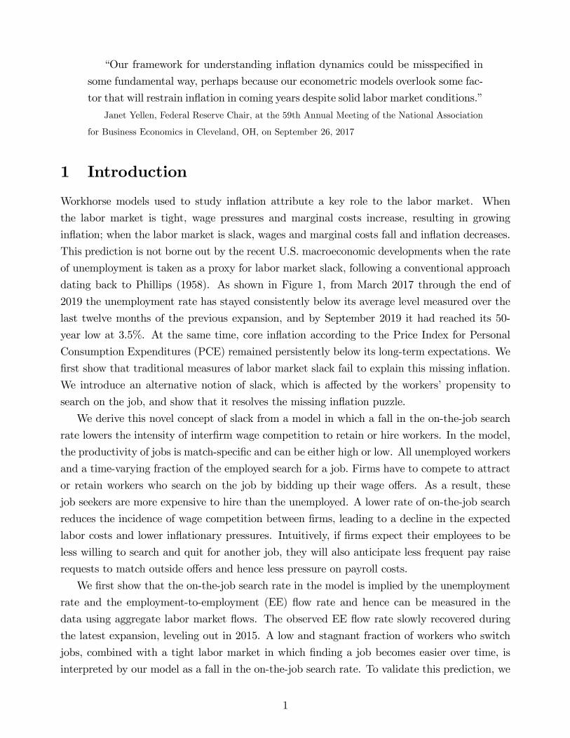
dating back to Phillips (1958). As shown in Figure 1, from March 2017 through the end of
2019 the unemployment rate has stayed consistently below its average level measured over the
last twelve months of the previous expansion, and by September 2019 it had reached its 50-
year low at 3.5%. At the same time, core inflation according to the Price Index for Personal
Consumption Expenditures (PCE) remained persistently below its long-term expectations. We
first show that traditional measures of labor market slack fail to explain this missing inflation.
We introduce an alternative notion of slack, which is affected by the workers’propensity to
search on the job, and show that it resolves the missing inflation puzzle.
We derive this novel concept of slack from a model in which a fall in the on-the-job search
rate lowers the intensity of interfirm wage competition to retain or hire workers. In the model,
the productivity of jobs is match-specific and can be either high or low. All unemployed workers
and a time-varying fraction of the employed search for a job. Firms have to compete to attract
or retain workers who search on the job by bidding up their wage offers. As a result, these
job seekers are more expensive to hire than the unemployed. A lower rate of on-the-job search
reduces the incidence of wage competition between firms, leading to a decline in the expected
labor costs and lower inflationary pressures. Intuitively, if firms expect their employees to be
less willing to search and quit for another job, they will also anticipate less frequent pay raise
requests to match outside offers and hence less pressure on payroll costs.
We first show that the on-the-job search rate in the model is implied by the unemployment
rate and the employment-to-employment (EE) flow rate and hence can be measured in the
data using aggregate labor market flows. The observed EE flow rate slowly recovered during
the latest expansion, leveling out in 2015. A low and stagnant fraction of workers who switch
jobs, combined with a tight labor market in which finding a job becomes easier over time, is
interpreted by our model as a fall in the on-the-job search rate. To validate this prediction, we
1
The Unemployment Rate
2010 2012 2014 2016 2018
4
5
6
7
8
9
10Civilian Unemployment Rate2007 Average Unemployment Rate
Figure 1: Labor market and inflation dynamics during the post-Great Recession recovery. The left panel: the civilian unemploy-ment rate (solid line) and its average computed over the 12 months that preceded the Great Recession (red dashed line). Source:Bureau of Labor Statistics (BLS). The right panel: core inflation according to the Price Index for Personal Consumption Expen-ditures (PCE) (black line). Average of monthly figures annualized in percentage. Source: Bureau of Economic Analysis (BEA).The red stars denote the 10-year ahead expectations about the PCE inflation rate. Source: Federal Reserve Bank of Philadelphia,Survey of Professional Forecasters. The shaded areas denote National Bureau of Economic Analysis (NBER) recessions.
estimate the on-the-job search rate at the micro level using the Survey of Consumer Expectations
(SCE) administered by the Federal Reserve Bank of New York. In the Survey, the on-the-job
search rate has fallen from 2014 through 2017 in a way that is remarkably similar to our measure
based on the aggregate labor market flows.
We derive a model-consistent concept of labor market slack, which can be measured using
the observed series of the unemployment rate and the EE rate. Labor market slack hinges on
the intensity of interfirm wage competition, which is shown to depend on (i) the unemployment
rate, (ii) the degree of cyclical labor misallocation (i.e., the incidence of low-productivity jobs),
and (iii) the on-the-job search rate. An increase in the rate of unemployment or a fall in the
fraction of workers who are searching on the job increase slack in the model because they raise
the firms’chances to fill their vacancies with unemployed workers, who are cheaper to hire,
as they are unable to prompt wage competition between employers. The more ineffi cient the
allocation of labor, the more likely it is for firms to meet workers employed in low-productivity
(bad) matches. Because enticing a worker away from a bad match is cheaper on average
than poaching a worker from a good match, labor misallocation lowers the intensity of wage
competition and raises labor market slack.
We then take the model to the unemployment rate and the EE flow rate observed in the
data and recover the two shocks that buffet the model economy: a shock to the on-the-job
search rate and a demand shock. The demand shock serves the sole purpose of generating the
fluctuations in the unemployment rate observed in the data. Given the unemployment rate,
the EE rate allows us to pin down the shocks to the on-the-job search rate, as described earlier.
We use the time series of the two shocks to simulate inflation and labor costs from the model.
2
We find that the model does not see inflationary pressures during the most recent expansion,
and this result is driven by the decline in the rate of on-the-job search, which has kept wage
competition at low levels. In addition, labor-cost dynamics in the model closely correlate with
the growth rate of average hourly earnings and the employment cost index.
We analyze the contribution of each of the three components of labor market slack to
inflation during the expansionary period following the Great Recession. We find that the drop
in the on-the-job search rate emerges as the key explanation for why inflation was so low in the
U.S. after nine years of economic recovery. Labor misallocation also contributes significantly
to keeping inflation persistently subdued following the Great Recession, offsetting the effects of
the low unemployment rate.
The surge in labor misallocation right after the recession was due to the exceptionally high
stock of unemployed workers who took a first step back onto the job ladder. As a result of
the persistent decline in the on-the-job search rate throughout the recovery, the speed at which
workers moved to better jobs fell, exacerbating labor misallocation and exerting persistent
downward pressures on wages and inflation. Indeed, our model predicts that after nine years of
expansion, a significant fraction of the employed workers is still stuck in suboptimal jobs. This
prediction is consistent with the micro evidence from the SCE, which shows that in 2017, after
eight years of economic recovery, about 30% of workers were not fully satisfied with how their
current jobs fit their experience and skills. This persistent rise in bad jobs also accords well
with evidence in Jaimovich et al. (2020), who show that a third of the workers that had been
employed in routinary occupations before the Great Recession could not find similar jobs and
were stuck in nonroutinary manual occupations.
In the post-war period, the U.S. economy experienced low rates of unemployment and in-
flation in other circumstances, for example in the 1960s and in the 1990s. However, these
episodes occurred in connection with high labor productivity growth, which in New Keyne-
sian (NK) models lowers real marginal costs and hence dampens inflationary pressures. What
made the latest expansion so puzzling was that inflation remained low while labor productivity
growth also slowed down (Fernald 2016). By predicting a persistent surge in the incidence of
low-productivity jobs in the latest expansion, our model reconciles the absence of inflationary
pressures with a dismal labor productivity growth.
How does the model fare in an earlier period? We address this question by comparing the
performance of our measure of labor market slack with that of other popular measures in the
literature– such as the labor share of income (as in Galí and Gertler 1999); the unemployment
gap based on the nonaccelerating inflation rate of unemployment (NAIRU); and the hours
worked, which features prominently in estimated dynamic general equilibrium models as the
key observable variable informing the output gap (e.g., Christiano, Eichenbaum, and Evans
2005). We find that in this earlier sample period (1990 through 2012), our measure of slack
3
performs comparably with these other popular measures while it does significantly better at
accounting for the missing inflation in the past decade.
The result that inflation was moderate in the latest expansion relies on the countercyclicality
of the search rate. When we extend the analysis back to the early 1990s, we find that the search
rate was countercyclical in this earlier period too. We show that such countercyclicality stems
from the fact that the volatility of the unemployment rate, which in the model reflects the
probability of finding a job, is higher than the volatility of the EE flow rate in the data.
We elaborate on the reasons why the on-the-job search rate is countercyclical by discussing a
number of findings in the empirical micro-labor literature.
Another anomaly with the behavior of inflation in the earlier decade is the observation that
it did not fall during the Great Recession as predicted by standard macroeconomic models
(Hall 2011; Ball and Mazumander 2011; Coibion and Gorodnichenko 2015, and Bianchi and
Melosi 2017). While we do not explicitly focus on this so-called missing deflation puzzle, the
countercyclicality of the on-the-job search rate dampens the countercyclicality of our measure
of slack compared with other traditional measures. Therefore, our measure does not predict
implausibly low inflation during the Great Recession, as traditional measures of slack do.
The assumption that the on-the-job search rate varies stochastically over time is meant
to capture all those cyclical factors that drive the decision to search on the job, as well as
compositional changes in the propensity to search within the pool of employed workers.1 We
do not explicitly model these compositional changes in our macro model and assume the on-the
job search is exogenous. We believe that this is the right approach at this stage given that a
theory of what drives this rate has yet to emerge. In addition, because the time series of the
on-the-job search rate is uniquely pinned down by observing the unemployment rate and the
EE flows, endogenizing this rate could change our results only by affecting agents’expectations
about the future evolution of the rate. We show that this expectation channel is not strong
enough to materially affect our quantitative results.
Our model features an occasionally binding zero lower bound (ZLB) constraint on the nom-
inal interest rates. Introducing this constraint is important given that the severity of the Great
Recession, which in our analysis is captured by the sharp increase of the unemployment rate in
2008 and 2009, drives the current and expected nominal interest rates to the ZLB for several
months in our model. We develop an innovative method to solve and simulate models when
the ZLB constraint is binding. Our method does not rely on assuming perfect foresight.
A voluminous literature has shown that inflation has become less sensitive to changes in the
traditional measures of labor market slack since the early 1990s, flattening out the slope of the
estimated price Phillips curve (Atkenson and Ohanian 2001; Stock and Watson 2007, 2008, and
1For instance, workers who are hired at the beginning of an expansion may be more dynamic than those whogenerally find jobs when the labor market is already very tight (Cahuc, Postel-Vinay, and Robin 2006).
4
2019).2 We see our paper as complementary to this literature. Indeed, we show that a flatter
Phillips curve in and of itself does not solve the puzzle of the persistently low inflation observed
in the past decade. To our knowledge, this is the first paper that explains the missing inflation.
Moscarini and Postel-Vinay (2019) pioneer a New Keynesian model in which cyclical labor
misallocation brings about deflationary pressures. In building our model, we draw from their
groundbreaking contribution. These scholars use the model to show that the degree of labor
misallocation is a better predictor of inflation than the rate of unemployment. Our contribution
differs from that of Moscarini and Postel-Vinay (2019) in two important respects. First, while
their empirical analysis is reduced form and external to their structural model, we take our
structural model to the data using time series methods. Second, while Moscarini and Postel-
Vinay focus exclusively on the role of cyclical labor misallocation, we emphasize the importance
of the propensity to search on the job for the dynamics of wages and inflation. We show that
this propensity can be measured using aggregate labor market flows and the macro estimates are
validated using micro data. Crucially, allowing the on-the-job search rate to vary over time is
key to explaining the missing inflation of the past decade. When the search rate is constant, the
acceptance ratio, which is the ratio of EE to UE flow rates, is a leading indicator for inflationary
pressures. This ratio is a proxy for the degree of cyclical labor misallocation and a low value
of this ratio predicts high inflation.3 Through the end of 2019, the acceptance ratio was lower
than its pre-Great Recession average in the data (see Appendix A). Our model jointly explains
this low acceptance ratio, the persistent increase in bad jobs, and the low inflation in the most
recent years with the decline in the incidence of on-the-job search. According to our model the
acceptance ratio is currently low in the data, not because employment is effi ciently allocated
but because fewer workers are searching on the job.
Understanding the search behavior of the employed using disaggregated labor data is an
active area of ongoing research. In this paper, we stress the importance of this line of research to
improve our understanding of inflation. Abraham and Haltiwanger (2019) survey this literature
and analyze the behavior of a measure of labor market tightness extended to include all effective
job seekers, including employed workers searching on the job. A fall in the rate of on-the-job
search, in their view, reduces the number of job seekers and thereby increases labor market
tightness, which in turn puts upward pressure on wage and price inflation. In our model, a fall
in the rate of on-the-job search instead reduces interfirm wage competition, thereby inducing
lower inflationary pressures.
The paper is organized as follows. In Section 2, we provide the motivation for our paper by
2McLeay and Tenreyro (2019) provide a intriguing theoretical reason for why the Phillips curve has becomeflatter in recent years.
3The fraction of accepted offers is lower when more workers are employed in high-productivity jobs. If workersare effi ciently allocated, outside offers are declined and matched by the current employer, raising productioncosts and inflation.
5
laying out the missing inflation puzzle. The model from which we derive the novel measure of
labor market slack is introduced in Section 3. We explain the empirical strategy and results in
Section 4. We discuss the performance of the proposed measure of slack in fitting inflation on a
longer sample starting in the early 1990s in Section 5. In Section 6, we present our conclusions.
2 The Missing Inflation Puzzle
The New Keynesian model is the most popular framework to study inflation. A key building
block of this framework is the New Keynesian Phillips curve, which posits that inflation πthinges on the expected dynamics of future real marginal costs ϕt:
πt = κϕt + βEπt+1, (1)
where κ denotes the slope of the curve and β the discount factor. In empirical applications, the
real marginal cost ϕt is proxied in a variety of ways. We consider proxies related to the following
three traditional theories of the Phillips curve: (i) old-fashioned theories (recently revived by
Galí, Smets, and Wouters 2011) that link inflation to the current and expected unemployment
gap; (ii) the standard New Keynesian theory (derived from models with no labor frictions),
which suggests that the labor share alone is the key determinant of the inflation rate (Galí
and Gertler 2000); (iii) a variant of the standard New Keynesian theory, based on models that
account for search and matching frictions, which explains inflation using current and expected
measures of the labor share as well as UE flow rates (Krause, Lopez-Salido, and Lubik, 2008).4
While there are more sophisticated versions of the New Keynesian Phillips curve, which, for
instance, feature price indexation, we focus here on the simpler version of this curve to facilitate
comparability with the model presented in the next section. We discuss the extension to the
case of price indexation in Appendix C and show that it does not affect our main conclusions.
By solving equation (1) forward, we can express expected inflation as the sum of the current
and future expected real marginal costs. We estimate a Vector Autoregression (VAR) model
to forecast the future stream of the three aforementioned measures of real marginal costs. The
forecasts of real marginal costs are launched from every quarter during the post-Great Recession
recovery and are then plugged into the Phillips curve, which returns the predicted inflation rate
by each of the three theories of marginal costs in every quarter of the recovery. To conduct this
exercise, we set the discount factor β to 0.99 (data are quarterly) and a slope of the Phillips
curve κ equal to 0.005, so as to fit inflation at the beginning of the post-Great Recession recovery
(2009—2011). The resulting Phillips curve is fairly flat and in line with estimates obtained by
Del Negro et al. (2020) for the U.S economy over the post-1990 period, using standard measures
4To make the paper self-contained, we summarize how this third series of marginal costs is constructed inAppendix B. We refer the interested reader to Krause, Lopez-Salido, and Lubik (2008) for more details.
6
2009 2010 2011 2012 2013 2014 2015 2016 2017
-1
-0.5
0
0.5
1
The Missing Inflation Puzzle
Unemployment GapLabor ShareLabor Market FrictionsData: Core PCE Inflation Gap
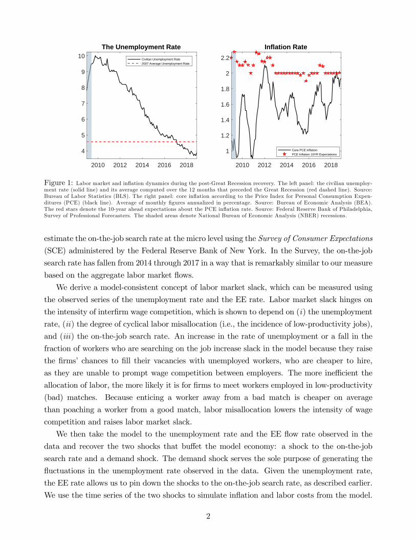
Figure 2: PCE core inflation gap from 2009Q1 through 2017Q3 and inflation dynamics predicted using three traditional theoriesof inflation.
of slack. While the slope of the Phillips curve affects the magnitude of inflation predicted by
the three measures of slacks, it does not affect the point in time when inflation rises above its
long-run level, which is what we are interested in (see Appendix C). A flatter Phillips curve in
and of itself does not explain why inflation has remained subdued for an entire decade.
To estimate the VAR model, we use the following observable variables: the labor share,
the job finding rate, real wages, the civilian unemployment rate, real gross domestic product
(GDP), real consumption, real investment, inflation according to the Consumer Price Index
(CPI), and the federal funds rate (FFR).5 We detrend the observable variables by using their
8-year past moving average trend. The only exception is when we construct the unemployment
gap, for which we use the short-term NAIRU estimates.6 We rely on the NAIRU estimates to
construct the unemployment gap as this practice is very popular in those studies whose object
is to estimate the Phillips curve. The sample period for estimation is from 1958Q4 through
2017Q4.
Figure 2 shows that all the three traditional theories of marginal costs predict that inflation
should have been above its long-run level (positive inflation gap) by the end of 2012. None of
these theories is able to account for why inflation stayed so low for so many years after the
Great Recession because all three proxies for marginal costs improved quickly in the first years
of the economic recovery. Consequently, the VAR model’s forecasts of future marginal costs
go up at a relatively early stage of the recovery, which leads the three New Keynesian Phillips
curves to predict inflation above its long-run level. As shown in Appendix E, a state-of-the-art
structural model, such as the model studied in Smets and Wouters (2007), also fails to explain
the missing inflation.
It is worth noting that this VAR approach is general and agnostic because we do not impose
5Details on how these series are constructed are in Appendix D.6Using the long-term NAIRU would not change our main conclusions.
7
a requirement that expectations about future labor costs are formed according to the Phillips
curve. Imposing such a restriction on the VAR structure may lead to misspecification that
would most likely worsen the quality of the forecasts of real marginal costs. That said, our main
conclusions are not affected by imposing this restriction, and our approach is more appealing
in that the unrestricted VAR model is a reduced-form, theory-free representation for the data
that is less prone to misspecification than structural theory-based models. Another advantage
of our approach is that (unrestricted) VAR models generally provide reliable macroeconomic
forecasts.7
3 A General EquilibriumModel with On-the-Job Search
The failure of the traditional measures of labor market slack to explain inflation in the past
decade motivates the need of an alternative concept of slack. We build this concept using a
New Keynesian model in which a time-varying fraction of workers search on the job and firms
have to compete to attract or retain these workers by bidding up their wage offers.8
3.1 The Economy
The economy is populated by a representative, infinitely lived household, whose members’labor
market status is either unemployed or employed. All members of the household are assumed to
pool their income at the end of each period and thereby consume the same amount. The labor
market is frictional and workers search for jobs whether they are unemployed or employed.
While all unemployed workers are also job seekers, it is assumed that any employed worker
can search in a given period with a probability st, which is assumed to follow an exogenous
first-order autoregressive AR(1) process with Gaussian shocks. Time variation in st is meant
to capture all those cyclical factors that are responsible for changes in the average rate of on-
the-job search in the data, including compositional changes in the propensity to search in the
pool of employed workers. Households trade one-period-government bonds Bt.
We distinguish two types of firms: labor-service producers and price setters. The service
sector comprises an endogenous measure of worker—firm pairs that match in a frictional labor
7For Bayesian VAR models to deliver reliable macro forecasts, the choice of the prior is key. We checkthat VAR forecasts are accurate in sample and follow the conventions established by the forecasting literature.Specifically, we use the unit-root prior introduced by Sims and Zha (1998) and choose the prior hyperparameters,which determine the direction of the Bayesian shrinkage, so as to maximize the marginal likelihood.
8Key empirical studies that explicitly allow for search and matching frictions in New Keynesian modelsinclude Gertler, Sala, and Trigari (2008), Krause, Lopez-Salido, and Lubik (2008), Ravenna and Walsh (2008)and Christiano, Eichenbaum, and Trabandt (2016). We deviate from these studies by considering the role ofon-the-job search and by focusing on inflation. Gertler, Huckfeldt, and Trigari (2019) develop a model whereproductivity is match-specific, and workers climb the ladder by searching on the job. Their paper abstractsfrom nominal rigidities and focuses on the wage cyclicality of the newly hired workers.
8
market and produce a homogeneous nonstorable good. Productivity y ∈ {yg, yb} is match-specific and can be either good or bad, with yg > yb > 0. We let ξg denote the probability
that upon matching the productivity draw is good and ξb = 1 − ξg the probability that the
draw is bad. The output of the match is sold to price-setting firms in a competitive market
at the relative price ϕt (the price of the labor service relative to that of the numeraire), and
transformed into a differentiated product. Specifically, one unit of the service is transformed
by firm i into one unit of a differentiated good yt (i). These firms set the price of their goods
subject to Calvo price rigidities. Households consume a bundle Ct of such varieties in order to
minimize expenditure. This bundle is the numeraire for this economy and its price is denoted
by Pt. The monetary authority sets the nominal interest rate of the one-period government
bond following a Taylor rule subject to a nonnegativity constraint. The fiscal authority levies
lump-sum taxes Tt to finance maturing government bonds.
3.2 The Labor Market
The labor market is frictional and governed by a meeting function that brings together vacancies
and job seekers. The pool of workers looking for jobs at each period of time t is given by the
measure of workers who are unemployed at the beginning of a period, u0,t plus a fraction st of
the workers who are employed, 1 − u0,t. Denoting the aggregate mass of vacancies by vt, we
can define labor market tightness as
θt =vt
u0,t + st (1− u0,t). (2)
We assume that the meeting function is homothetic, which implies that the rate at which
searching workers find a vacancy, φ (θ) ∈ [0, 1], and the rate at which vacancies draw job seekers,
φ (θ) /θ ∈ [0, 1], depend exclusively on θ and are such that dφ (θ) /dθ > 0 and d [φ (θ) /θ] /dθ < 0.
Because of frictions in the labor market, wages deviate from the competitive solution. It
is assumed that wage bargaining follows the sequential auction protocol of Postel-Vinay and
Robin (2002). Namely, the outcome of the bargaining is a wage contract, i.e., a sequence of
state-contingent wages, which promises to pay a given utility payoff in expected present value
terms (accounting also for expected utility from future spells of unemployment and wages paid
by future employers). The commitment of the worker—firm pair to the contract is limited, in the
sense that either party can unilaterally break up the match if either the present value of firm
profits becomes negative or the present value utility from being employed falls below the value
of being unemployed. The contract can be renegotiated only by mutual consent: if an employed
worker meets a vacancy, the current and the prospective employer observe first the productivity
associated with both matches, and then engage in Bertrand competition over contracts. The
worker chooses the contract that delivers the largest value.
9
The within-period timing of actions is as follows: all the unemployed workers and a fraction
st of the employed search for a job at the beginning of the period. Next, some workers move
out of the unemployment pool, while successful on-the-job seekers have their wage renegotiated
and possibly move up the ladder. Then production takes place and wages are paid. This timing
implies that workers who are unemployed at the beginning of the period can produce at the end
of the same period if they find a job. And similarly, workers who are employed at the beginning
of the period may be producing in a different job at the end of the same period if they switch
employers. Finally, a fraction δ of the existing matches is destroyed.
These assumptions imply the following dynamics for the aggregate state of unemployment.
Denote the stock of end-of-period employed workers as
nt = 1− ut. (3)
Aggregate unemployment at the beginning of a period is given by
u0,t = ut−1 + δnt−1, (4)
while aggregate unemployment at the end of a period is given by
ut = u0,t [1− φ (θt)] . (5)
3.3 Households
Households solve two problems. First, they decide how to optimally allocate their consumption
of the aggregate good over time. Second, they solve an intratemporal problem to optimally
choose the composition of the aggregate good in terms of differentiated goods sold by the price
setters. All workers share their consumption risk within the households, allowing us to solve
the problems from the perspective of a representative household.
The intertemporal maximization problem The representative household enjoys utility
from the consumption basket Ct and from the fraction of its members who are not working and
are therefore free to enjoy leisure. The parameter b controls the marginal utility of leisure. We
assume that the utility function is logarithmic in consumption and let µt denote the preference
shock to consumption, which is assumed to follow a Gaussian AR(1) stochastic process in logs.
The resources available to consume at a given point in time t include government bond holdings
Bt; profits from the price setters, which sell differentiated goods, DPt ; profits from the service
firms DSt ; wages from the workers who are employed; and transfers from the government Tt.
We assume that all unemployed workers look for jobs, and restrict our attention to equilibria
where the value of being employed for any worker is no less than the value of being unemployed.
10
In this setup, the measure of workers who are employed is not a choice variable of the household,
but is driven by aggregate labor market conditions through the job finding probability φ (θt).
Let et (j) ∈ {0, 1} be an indicator function which takes the value of one if a worker j is employedafter worker reallocation takes place, but before the current-period exogenous separation occurs
with probability, δ, and zero otherwise. The intertemporal maximization problem is
max{Ct,Bt+1}
E0
∞∑t=0
βt[µt lnCt + b
∫ 1
0
(1− et (j)) dj
],
subject to the budget constraint,
PtCt +Bt+1
1 +Rt
≤ Bt +
∫ 1
0
et (j)wt (j) +DPt +DS
t + Tt,
and the stochastic process for the employment status,
prob {et+1 (j) = 1 | et (j)} = et (j) [(1− δ) + δφ (θt+1)] + [1− et (j)]φ (θt+1) (6)
prob {et+1 (j) = 0 | et (j)} = 1− prob {et+1 (j) = 1 | et (j)} ,
and for equilibrium wages wt (j).9
Equation (6) implies that a worker who is registered as unemployed at the production stage
of period t, i.e., et (j) = 0, will only have a chance to look for jobs at the beginning of next
period, and get one with probability φ (θt+1). Moreover, a worker employed at time t, i.e.,
et (j) = 1, will also be in employment at t + 1 if she does not separate from the current job
between periods at the exogenous rate δ, or if she separates but manages to find a new job with
probability φ (θt+1) in the next period.
The intratemporal minimization problem conditions Households minimize total ex-
penditure on all differentiated goods,
minqt(i),i∈[0,1]
∫ 1
0
pt (i) qt (i) di, (7)
9The evolution of individual wages must obey the wage contract negotiated by the worker—firm pair. In thesenegotiations, workers and firms agree on a present discounted value of the future stream of utility, as we willshow later. However, there are many streams of wages that can deliver the promised present discounted value ofutility, making the distribution of the individual wages indeterminate. It can be shown that this indeterminacyis inconsequential for aggregate equilibrium outcomes. Nevertheless, as we will clarify later, the real marginalcost, which is the price of the labor service and hence a measure of the average cost of labor, is determined,even though the underyling wage distribution is not.
11
subject to the general Kimball (1995) aggregator assumed in Smets and Wouters (2007):∫ 1
0
G (qt (i) /Qt) di = 1. (8)
The reason why we choose this particular aggregator will be explained in Section 4.1, where
we discuss how we calibrate the key parameter of this aggregation technology. As in Dotsey
and King (2005), Levin, Lopez-Salido, and Yun (2007), and Lindé and Trabandt (2018), we
assume the following strictly concave and increasing function for G (qt (i) /Qt):
G (qt (i) /Qt) =ωk
1 + κ
[(1 + κ)
qt (i)
Qt
− κ] 1
ωk
+ 1− ωk
1 + κ, (9)
where ωk = χ(1+κ)1+κχ , κ ≤ 0 is a parameter that governs the degree of curvature of the demand
curve for the differentiated goods and χ captures the gross markup.
The solution of this expenditure minimization problem is the demand function for the dif-
ferentiated good (i):qt (i)
Qt
=1
1 + κ
(Pt (i)
PtΞt
)ι+
κ1 + κ
, (10)
where κ ≤ 0 is a parameter, ι = χ(1+κ)1−χ , Ξt is the Lagrange multiplier associated with the
constraint (8), and the aggregate price index (i.e., the price of the numeraire) satisfies 1 =∫ 1
0
(pt,iPtΞt
) ι
ωk
di.
3.4 Price Setters
Price setters buy the (homogeneous) output produced by the service firms in a competitive
market at the relative price ϕt, turn it into a differentiated good, and sell it to the households
in a monopolistic competitive market. They can re-optimize their price Pt(i) with a period
probability 1−ζ. If they cannot reoptimize, they adjust their price at the steady-state inflationrate Π. Therefore, the problem of the price setting firm is expressed as follows:
maxPt+s(i)
Et
∞∑s=0
βt+sζsλt+sλt
(Pt(i)Π
s − Pt+sϕt+s)qt+s(i), (11)
subject to the demand function (10). Log-linearization and standard manipulations of the
resulting price-setting equation lead to the purely forward-looking New Keynesian Phillips
curve, which was shown in equation (1).
As standard in New Keynesian models, the Calvo lottery makes this price-setting problem
dynamic; i.e., price setters that are allowed to re-optimize their price at time t find it optimal to
forecast the future stream of real marginal costs {ϕτ}∞τ=t. This is because price setters anticipate
12
that they may not be able to re-optimize their price in the next periods. In our model, the price
setters’real marginal costs ϕt coincide with the relative price of the labor service, and hence,
the optimizing price setters care about the determinants of that price, which are the focus of
the next section.
3.5 Service Sector Firms: Free-Entry Condition
In this section, we introduce the free-entry condition to the labor service firm and discuss the
pivotal role played by this condition in determining the dynamics of price setters’marginal
costs and inflation in the model. This condition implies that entrant firms will make zero
profits in expectations; i.e., expected costs are equal to the expected surplus after the match is
formed. We first discuss the expected costs incurred by entrant service sector firms and then
the expected surplus.
Service firms have to pay an advertising cost c per period. In addition, to form a match and
produce, they also have to pay a sunk fixed cost of hiring cf . The expected cost of creating a
job equals cf + c$t, where $t is the vacancy filling rate and $−1 measures the expected number
of periods that is required to meet a worker.
The expected return from a match depends on whether the worker matched is employed
or unemployed. Following Postel-Vinay and Robin (2002) and Moscarini and Postel-Vinay
(2018, 2019), it is assumed that unemployed workers have no bargaining power, so the firm
will appropriate the entire surplus of the match, which will in turn depend on its quality. If
the firm meets an employed worker instead, the firm engages in Bertrand competition with the
incumbent firm in an attempt to poach the worker away from the current match. An important
implication of these assumptions is that an increase in wages is not necessarily backed by a rise
in workers’productivity. This can happen, for instance, when a worker renegotiates upward
the value of a contract, as their employer agrees to match the offer of a poaching firm. This
temporary decoupling between wages and the worker’s productivity is key for the job ladder to
have meaningful implications for inflation. As we will show, these assumptions also imply that
the worker’s ability of extracting more and more surplus from a match depends on her position
on the job ladder.
While the assumption that unemployed workers have no bargaining power is undoubtedly
stark, it provides tractability, allowing for an analytical characterization of the expected sur-
pluses that appear in the free-entry condition. Such an analytical characterization turns out to
be very useful in providing intuition about the link between the labor market and inflation in
the model, which will be the focus of Section 3.6.
More importantly, this assumption breaks the link between labor market tightness and
wages, allowing us to isolate the effects of searching on the job on firms’wage competition.
Specifically, a drop in the on-the-job search rate leads to a fall in the share of job seekers that
13
are employed, thereby reducing interfirm wage competition and the cost of labor service. This
is the first paper that focuses on this channel to explain inflation. Indeed, in a standard New
Keynesian model with search and matching, a fall in the rate of on-the-job search reduces the
number of job seekers, increasing labor market tightness and wages. For instance, this channel
is emphasized in Abraham and Haltiwanger (2019) and in most of the reduced-form labor
literature reviewed in that paper. Our model-based empirical analysis is therefore constructed
to derive a simple measure of slack that isolates the role of interfirm wage competition and
investigate how far it can go in explaining the recent dynamics of inflation.
To illustrate how Bertrand competition works in our model, let y and y′ denote the match
quality with the incumbent and the poaching firm, respectively. We distinguish three possible
contingencies.
1. y = yg and y′ = yb. In this case the poaching firm is a worse match for the worker.
Bertrand competition implies that the incumbent firm will retain the worker and poaching
is not successful. If the worker was hired from a state of unemployment, she appropriates
the surplus St (yb) because Bertrand competition forces the incumbent to pay the worker
the highest value the poaching firm is willing to pay her. If the worker was not hired from
a state of unemployment, there is no change in the value of her contract.
2. y = y′ for y ∈ {yb,yg}. Match quality is the same for the two firms, and the worker will beindifferent between switching jobs or staying. We assume that switching takes place with
probability ν (a nonzero value for this parameter is required to match the high churning
rate in the U.S. labor market when calibrating the model’s steady-state parameters). In
either case, the firm that ends up with the worker relinquishes all the surplus St (y).
3. y = yb and y′ = yg. Match quality is lower with the incumbent firm, so the worker is
poached. Bertrand competition implies that the worker is given the highest surplus the
incumbent firm is willing to pay her, i.e., St (yb). The poaching firm’s surplus is therefore
the residual value of the match: St (yg)− St (yb) .
To sum up, entrant labor service firms can get a nonzero surplus from meeting an employed
worker only if the worker is in a bad match and the firm is a good match for the worker. As a
result, the free-entry condition can be written as follows:
cf +c
$t
=u0,t
u0,t + st (1− u0,t)
{ξbSt (yb) + ξgSt (yg)
}(12)
+st (1− u0,t)
u0,t + st (1− u0,t)
{ξg
l0b,t1− u0,t
[St (yg)− St (yb)]
},
where l0b,t denotes the measure of workers who, at the beginning of period t, are employed
in low-quality matches (l0b,t + l0g,t + u0,t = 1) and st is the on-the-job search rate. The term
14
st (1− u0,t) denotes the measure of employed workers searching on the job at the beginning of
period t, and u0,t + st (1− u0,t) is the measure of all job seekers at the beginning of period t.
The left-hand side is the expected costs of posting a vacancy, which has been discussed
above. The expected return from forming a match, on the right-hand side, depends on the
employment status, on the quality of the meeting, and, in the case the firm meets an employed
worker, also on the quality of the existing match. Three contingencies will give a nonzero surplus
to the firm and will hence appear in the right-hand side of the free-entry equation (12). The
expected return on the right-hand side is just an average of the surplus accrued in these three
contingencies weighted by their respective probabilities.
The first contingency is when the entrant firm meets an unemployed job seeker, with prob-
ability u0,t/[u0,t + st (1− u0,t)], and the job seeker is a bad match for the firm, with probability
ξb. In this case the meeting gives the firm the surplus St (yb). The second contingency is when
the entrant firm meets an unemployed job seeker who turns out to be a good match, with
probability ξg, providing the firm with the surplus St (yg). These two expected returns appear
in the first term on the right-hand side of the free-entry equation (12). The third contingency,
i.e., the second term in the right-hand side of the free-entry equation (12), occurs when the firm
meets an employed worker, with probability st (1− u0,t) / [u0,t + st (1− u0,t)], and the following
two conditions are met: (i) the worker is a good match for the entrant firm, which occurs with
probability ξg, and (ii) the worker is currently in a bad match, which happens with probability
ξgl0b,t/ (1− u0,t).10 As explained above, this is the only case in which an entrant firm can extract
a nonzero surplus from meeting with an employed worker.
Moscarini and Postel-Vinay (2019) show that the surplus function can be written as follows
St (y) = yWt −bλ−1
t
1− β (1− δ) , (13)
where λt is the Lagrange multiplier with respect to the household’s budget constraint and
Wt = ϕt + β (1− δ)Etλt+1
λtWt+1. (14)
See Appendix F for details on the derivations in the context of our model. From the point of
view of a labor service firm, Wt can be interpreted as the expected present discounted value of
the entire stream of current and future prices at which the homogeneous good is sold by the
firm until separation from the worker.
10Note that l0b,t denotes the share of workers that are employed in a bad match at the beginning of the period.We rescale this share by the fraction of employed workers at the beginning of the period (1 − u0,t) so as toobtain the conditional probability of meeting a bad match.
15
3.6 Wage Competition, Labor Market Slack, and Inflation
In this section, we conduct a partial-equilibrium thought experiment to build intuition about
what are the main drivers of inflation in the model. We will verify this intuition later in Section
4.4. In this thought experiment, we consider the free-entry condition (12) in isolation and
assume that either the unemployment rate u0t increases, the fraction of workers in a bad match
l0b,t rises, or employed workers search less frequently (st decreases). The direct effect of these
changes on the free-entry condition is to increase the expected profits (i.e., the right-hand side
of the free-entry condition) because it is more likely for firms to meet a worker they can extract
a positive surplus from. As a result, more firms want to enter the labor service sector enticed
by the expected gains from posting a vacancy.
Two variables adjust to restore the free-entry condition. On the one hand, the increase in
vacancies leads to a decrease in the vacancy filling rate, $t, and to an increase in the expected
cost of entry (i.e., the left-hand side of equation (12)). On the other hand, the expected
discounted stream of the relative price of labor service Wt falls, lowering surpluses St (y) as
implied by equations (13) and (14) and further dissuading firms from posting new vacancies
until the free-entry condition is satisfied. This drop in the relative price of labor service causes
price setters’marginal costs to fall, lowering inflation.11 As it will become clear later, the second
channel turns out to be important in the calibrated model.
Based on this reasoning, we conjecture that a key variable that affects inflation in the model
is the probability that, conditional on a contact, firms entering the labor service sector are not
engaged in a wage competition that leads them to relinquish the entire surplus to the worker.
This probability is defined as follows:
Σt ≡u0,t
u0,t + st (1− u0,t)+
st (1− u0,t)
u0,t + st (1− u0,t)ξg
l0b,t1− u0,t
, (15)
where the first term on the right-hand side is the probability of meeting an unemployed worker
and the second term is the probability of meeting a worker employed in a bad match, who is
searching on the job, and turns out to be a good match for the poaching firm.
As explained in the partial-equilibrium thought experiment, a high value of this probability
implies a low intensity of wage competition, leading to downward pressures on price setters’
marginal costs and inflation. Hence, this probability can be thought of as a measure of labor
market slack in this model. While this intuition is obtained using this partial-equilibrium
thought experiment, the link between this measure of slack Σt and inflation also holds in
general equilibrium, as we will show in Section 4.4.
11The present discounted stream of real marginal costs Wt falls only in the presence of nominal rigidities.With flexible prices, real marginal costs are constant and the equilibrium of the free-entry condition is restoredonly through a change in the vacancy filling rate.
16
The notion of labor market slack provided in Equation (15) has two main advantages. First,
it will allow us to decompose inflation into three main drivers: the unemployment rate u0,t, the
degree of labor misallocation l0b,t, and the on-the-job search rate st. Such a decomposition will
turn out to be very useful to illustrate what are the key variables allowing the model to explain
the low inflation of the past decade. Second, we do not need to solve the model to quantify this
measure of labor market slack. In fact, it can be measured directly from the unemployment
rate and the EE flow rate in the data, as we will show in Section 4.3.
In the above equations, we let lb,t and lg,t denote the end-of-period measure of bad and
good matches, respectively. We let l0b,t and l0g,t denote beginning-of-period values. In turn, lb,t
is equal to the sum of the bad matches at the beginning of a period that did not move up
the ladder by finding a high-quality match within the period,[1− stφ (θt) ξg
]l0b,t, plus the new
hires from the unemployment pool who turned out to draw a low-quality match, φ (θt) ξbu0,t.
Indeed, job-to-job flows from bad- to good-quality matches are given by the fraction of badly
matched employed workers, l0b,t, who search on the job with exogenous probability st, meet a
vacancy with probability φ (θt), and draw a good match with probability ξg.
The end-of-period measure of good matches is instead given by the beginning-of-period
measure of good matches l0g,t, plus the job-to-job inflows from bad matches stφ (θt) ξgl0b,t, and
the unemployed hired in a good job, φ (θt) ξgu0,t. Using the identity l0i,t+1 (y) = (1− δ) li,t (y)
for i = {b, g} ,we can rewrite the dynamic equations (16) and (17) to express the laws of motionfor bad and good jobs at their beginning-of-period values:
l0b,t+1 = (1− δ){[
1− stφ (θt) ξg]l0b,t + φ (θt) ξbu0,t
}, (18)
l0g,t+1 = (1− δ){l0g,t + stφ (θt) ξgl
0b,t + φ (θt) ξgu0,t
}. (19)
3.8 Policymakers and Market Clearing
The fiscal authority levies lump-sum taxes to repay its maturing bonds in every period. The
monetary authority follows a Taylor rule when the nominal interest rate Rt is not constrained
17
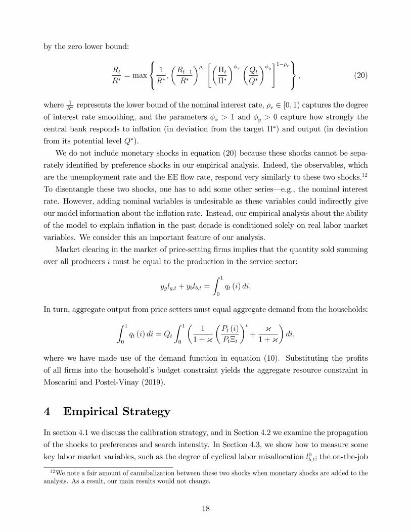
by the zero lower bound:
Rt
R∗= max
1
R∗,
(Rt−1
R∗
)ρr [(Πt
Π∗
)φπ (Qt
Q∗
)φy]1−ρr , (20)
where 1R∗ represents the lower bound of the nominal interest rate, ρr ∈ [0, 1) captures the degree
of interest rate smoothing, and the parameters φπ > 1 and φy > 0 capture how strongly the
central bank responds to inflation (in deviation from the target Π∗) and output (in deviation
from its potential level Q∗).
We do not include monetary shocks in equation (20) because these shocks cannot be sepa-
rately identified by preference shocks in our empirical analysis. Indeed, the observables, which
are the unemployment rate and the EE flow rate, respond very similarly to these two shocks.12
To disentangle these two shocks, one has to add some other series– e.g., the nominal interest
rate. However, adding nominal variables is undesirable as these variables could indirectly give
our model information about the inflation rate. Instead, our empirical analysis about the ability
of the model to explain inflation in the past decade is conditioned solely on real labor market
variables. We consider this an important feature of our analysis.
Market clearing in the market of price-setting firms implies that the quantity sold summing
over all producers i must be equal to the production in the service sector:
yglg,t + yblb,t =
∫ 1
0
qt (i) di.
In turn, aggregate output from price setters must equal aggregate demand from the households:∫ 1
0
qt (i) di = Qt
∫ 1
0
(1
1 + κ
(Pt (i)
PtΞt
)ι+
κ1 + κ
)di,
where we have made use of the demand function in equation (10). Substituting the profits
of all firms into the household’s budget constraint yields the aggregate resource constraint in
Moscarini and Postel-Vinay (2019).
4 Empirical Strategy
In section 4.1 we discuss the calibration strategy, and in Section 4.2 we examine the propagation
of the shocks to preferences and search intensity. In Section 4.3, we show how to measure some
key labor market variables, such as the degree of cyclical labor misallocation l0b,t; the on-the-job
12We note a fair amount of cannibalization between these two shocks when monetary shocks are added to theanalysis. As a result, our main results would not change.
18
CalibrationParameters Description Value Target/source
Parameters that affect the steady stateβ Discount factor 0.9987 Real rate 1.5%. (FOMC SEP)φ0 Scale parameter matching fn 0.3284 Job finding rate - Shimer (2005)δ Job separation rate 0.0200 Unemployment rate (100u0,t) 5.5%yb Productivity bad matches 1.0000 Normalizationyg Productivity good matches 1.0800 Faberman et al. (2019)ν Prob. of job switching if indifferent 0.5000b Utility of leisure 0.8082 Calibratedc Flow cost of vacancy 0.0124 Calibratedcf Fixed cost of hiring 0.4958 Calibrateds On-the-job search rate 0.2598 Calibratedξg Probability draw good match 0.2800 Calibratedχ Markup parameter 1.2000 20% markupκ Scale param. Kimball aggregator 10.0000 Smets and Wouters (2007)ζ Calvo price parameter 0.9250 Quarterly probability is 80%Π Steady-state gross inflation rate 1.0017 Net inflation rate of 2% p.a.ρr Taylor rule smoothing parameter 0.8500 Conventionalφπ Taylor rule response to inflation 1.8000 Conventionalφy Taylor rule response to output 0.2500 Conventionalψ Elasticity of matching function 0.5000 Moscarini and Postel-Vinay (2018)ρµ Autocorrel. preference shock 0.8000 Fixed
100σµ St. dev. preference shock 0.5883 Volatility of the unempl. rateρS Autocorrel. job search rate 0.9157 Maximum likelihood estimation
100σS St. dev. of job search rate shocks 2.5510 Maximum likelihood estimationVariable Description Value Target/source
Steady-state calibration targetsc$/c
f Ratio of variable to fixed cost 0.0780 Silva and Toledo (2009)
EE ≡ sφ[l0b(ξbν+ξg)+l0gξgν]
l0b+l0g
EE transition rate 0.0258 Pre-Great Recession EE rate
θ Labor market tightness 1.000 Normalizationl0g
l0g+l0b
Employment share in good jobs 0.6800 Employment share at top 10% firms(vtc+cfφt[u0,t+st(1−u0,t)])/H
ϕ Hiring costs over wages 0.6000 Hiring costs equal 2 weeks of wages
Table 1: Calibrated values for model parameters. Notes: FOMC SEP stands for the Federal Open Market Committee’s Summaryof Economic Projections. EE stands for employment-to-employment.
search rate; and our measure of labor market slack Σt, which we introduced in Section 3.6, using
the observed unemployment rate and the EE flow rate. In Section 4.4, we verify the conjecture
about the link between our measure of slack Σt and inflation. We present the main results of
the paper in Section 4.5. In Section 4.6 we present the micro evidence on the behavior of the
on-the-job search rate and use it to validate the rate measured by using aggregate labor market
flows.
4.1 Calibration
We calibrate the steady state of the model to the U.S. economy at monthly frequencies. To
do so, we assume a Cobb-Douglas matching function Mt = φ0 [u0,t + st (1− u0,t)]1−ψ vψt , where
19
ψ ∈ (0, 1) is an elasticity parameter and φ0 > 0 is a scale factor.
The calibration of the steady state requires assigning values to the following 11 parameter
values: β, φ0, δ, yb, yg, ν, b, ξg, c, cf and s. We set the discount factor β to match an annual real
interest rate of 1.5%, which is in line with the median of individual economic projections about
the real long-term interest rate from various Federal Reserve’s Board members, Federal Open
Market Committee (FOMC) members, or FOMC participants (known as Summary of Economic
Projections, or SEP).13 We normalize θ to unity, which allows us to pin down the scale factor
φ0, so as to match a job finding rate of 33 percent, which is the average of the job finding
rate computed following Shimer (2005) over a recent span of 25 years (January 1993-December
2018).14 The job separation rate δ is implied by the Beveridge curve, under the assumption
of a steady-state rate of unemployment of 5.5%. Namely, solving the Beveridge curve for
δ = φ0u01−u0+φ0u0
yields a separation rate of 0.02. The productivity of a bad match is normalized
to one, and the productivity in a good match is set to be 8% higher. We regard this productivity
differential as conservative, in the light of values that have been assigned in the calibration of
other comparable models with on-the-job search. Our targeted wage differential is in line
with evidence from Faberman et al. (2019) based on the Survey of Consumer Expectations,
which shows that wage gains associated with job switching are about 8%, after controlling
for observable characteristics of workers and jobs. Moreover, we noticed that assigning higher
values would violate the incentive compatibility constraint, which requires that the surplus of
bad matches should be positive both in steady state and in all periods of the sample used to run
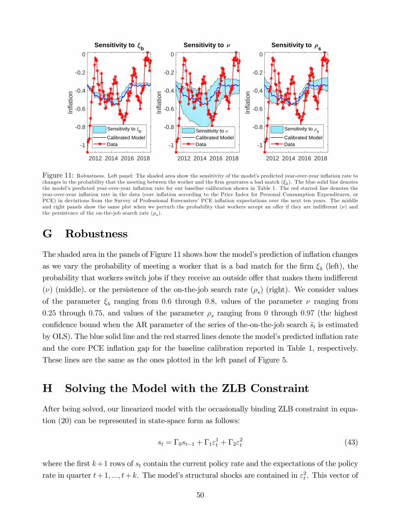
the empirical exercise of Section 4.5. Finally, we set the probability that workers will accept an
equally valuable outside offer to be ν = 0.5. This value is large enough to allow the model to
match the average EE flow rate in the U.S. economy. In Appendix G, we show that perturbing
the value of ν does not materially affect our results.
This leaves us with five parameters to calibrate: the parameter governing the utility of
leisure b, the probability of drawing a good match ξg, the flow cost of advertising a vacancy c,
the fixed cost of hiring cf , and the parameter governing search intensity s. These are calibrated
in order to match the following: (i) A value of expected hiring costs, including both the variable
and the fixed cost component, equal to two weeks of wages.15 (ii) A fraction of good jobs in
steady state equal to 67%, which is the share of employment for the top 10% U.S. firms by
employment size in the year 2000. (iii) A normalized value of labor market tightness equal to
one. (iv) A ratio of total variable costs of hiring to fixed costs c$/cf equal to 0.078. This value
is the ratio of pre-match recruiting, screening, and interviewing costs to post-match training
costs in the U.S., following the analysis of Silva and Toledo (2009)– which is based on the 1982
13We take the average of these projections from the FOMC meeting of May 2012– the first meeting afterwhich the projections were released– through the meeting of December 2019.14Under the assumption of unitary tightness (θ = 1), the job finding rate becomes equals to φ0.15The average wage is measured as the price of the labor service ϕ.
20
Employer Opportunity Pilot Project (EOPP), a cross-sectional firm-level survey that contains
detailed information on both pre-match and post-match labor turnover costs in the United
States.16 (v) A monthly job-to-job transition rate of 2.5841%, which is the average EE rate
(spliced using the quit rate as explained in Section 4.3) measured in the pre-Great Recession
sample (April 1990 through December 2007). We note that the value of the parameter s implied
by the calibration, 0.2598, is very close to the value of 0.22, which corresponds to the fraction
of U.S. workers who engage in on-the-job search every month, as measured using survey data
by Faberman et al. (2019). We have checked that the value of b implied by the calibration
is consistent with a positive surplus for low-quality matches both in steady state and in every
month considered in the empirical exercise of Section 4.5.
The calibration of the probability of a good match ξg (conditional on receiving a job offer)
relies on the empirical strategy in Moscarini and Postel-Vinay (2016), who exploit the notorious
correlation between firm size and productivity by assuming that employed workers climb the
ladder when moving to larger firms. In Appendix G we show that our main results are not
affected by reasonable variations in the probability of meeting a good match ξg.
We set the smoothing coeffi cient of the Taylor rule to the value of 0.85, which corresponds
to a coeffi cient of around 0.65 in quarterly space, and the response parameters to inflation and
output to the values of 1.8 and 0.25, respectively. The parameter χ is set to equal 1.2, which
implies a 20% price markup. The steady-state gross rate of inflation is set to equal 1.0016,
which implies a central bank’s inflation target Π∗ of 2% inflation annually in line with the
Federal Reserve’s stated inflation objective. Finally, we set the elasticity of vacancies in the
matching function ψ to equal 0.5 to be consistent with estimates by Moscarini and Postel-Vinay
(2018), which account for workers searching on the job.
The slope of the Phillips curve is determined by the scale parameter of the Kimball ag-
gregator κ and the Calvo parameter ζ, which govern the size of price stickiness. The formerparameter is set to 10 as in Smets and Wouters (2007). The latter is set to 0.925, which in
quarterly frequency implies a probability of not being able to reoptimize prices equal to 0.8.
We set the Calvo parameter so that the implied slope of the Phillips curve allows the model to
fit inflation at the beginning of the post-Great Recession recovery (2009—2011), following the
approach used to calibrate the slope of the Phillips curve in Section 2, where we evaluate the
ability of the traditional measures of slack to explain the missing inflation of the past decade.
The Kimball aggregator allows us to obtain the targeted value for the slope of the Phillips
curve without requiring us to assume an implausibily large degree of price stickiness. Indeed,
in the early stages of the recovery, the combined effect of the fall in the on-the-job search rate,
the binding ZLB constraint, and the persistent negative demand shocks that caused the Great
16Silva and Toledo (2009) indicate in Table 1 (p.80), that the average pre-match recruiting cost costs is $105.1,while the average post-match training cost amounts to $1,359.4.
21
Recession is to raise our measure of slack by a fair amount, requiring a relatively flat Phillips
curve to fit the level of inflation in that period. It is worth noting that while the slope of the
Phillips curve affects the magnitude of inflation predicted by the model, it can be shown to
have negligible effects on the point in time when the model predicts inflation to rise above its
long-run level, which is the central object of our analysis.
As we will show in Section 4.3, we can use the observed unemployment rate and the EE flow
rate in combination with a subset of model equations to obtain the time series of the on-the-job
search rate. This series can be retrieved from the data with no need to solve the model. To
pin down this series, we just have to take a stand on a few steady-state parameters (e.g., the
steady-state job finding rate φ and the separation rate δ), which we calibrate using the values
shown in Table 1. We use this series to estimate the persistence parameter ρS and the standard
deviation σS via maximum likelihood.
Turning to the parameters affecting the persistence and the volatility of the preference
shock, we set the autocorrelation parameter ρµ to 0.80 and then we calibrate the standard
deviation σµ so that the model can match the volatility of the observed unemployment rate in
the data (April 1990 through December 2018).17 The value of the autocorrelation parameter
is a bit lower than what is needed to fit the persistence in the U.S. civilian unemployment
rate. However, a persistence higher than 0.8 would make this shock propagate as a supply
shock moving the unemployment rate and inflation in the same direction.18 Because the other
shock (i.e., the shock to the on-the-job search rate) propagates as a supply shock, the model
would lack a demand shock to explain periods in which inflation and the unemployment rate
negatively comove.
Model Solution with the Zero Lower Bound (ZLB) Constraint The model is log-
linearized around its steady-state equilibrium.19 However, the zero lower bound introduces a
nonlinearity that prevents us from solving the model with standard solution methods. We
develop a novel method to find the certainty-equivalence solution to these temporarily non-
linear dynamics. Our method does not require us to assume that agents in the model have
perfect foresight. Agents update their rational expectations about the duration of the zero
lower bound over time after having observed past and current shocks.
Our method relies on appending a sequence of anticipated shocks (dummy shocks) to the
unconstrained Taylor rule. Anticipated shocks are known by agents in the current period, but
these shocks will hit the economy in future periods. The sequence of these shocks is computed
17We pick the unemployment rate as a target variable because it will be used in our main empirical exercise.18If a negative preference shock is very persistent, the fall in vacancy creation becomes so large that it generates
a sharp and prolonged contraction in the supply of the service, which in turn implies a persistent increase in itsprice, i.e., the real marginal cost ϕt. Moreover, the rise in current and future expected marginal costs entails arise in the rate of inflation, together with a contraction in aggregate production.19Rates and shares are linearized; all the other variables are log-linearized.
22
0 20 40 60-0.04
-0.02
0Unemployment Rate
0 20 40 60-0.1
-0.05
0Inflation Rate
0 20 40 60
-0.06
-0.04
-0.02
0Interest Rate
0 20 40 600
0.5
1
Fraction of Unemployed Job Seekers
0 20 40 600
0.1
0.2
0.3
Bad Matches
0 20 40 60
-0.3
-0.2
-0.1
0Good Matches
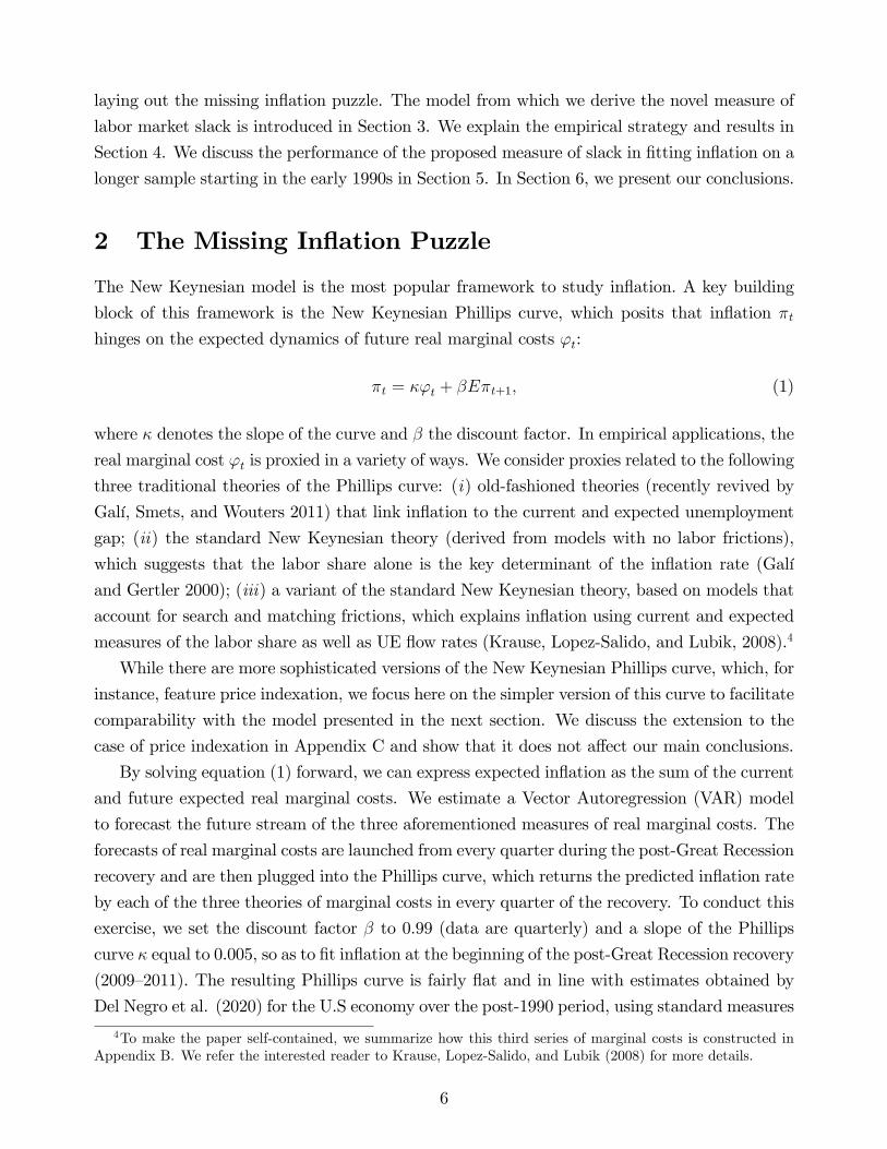
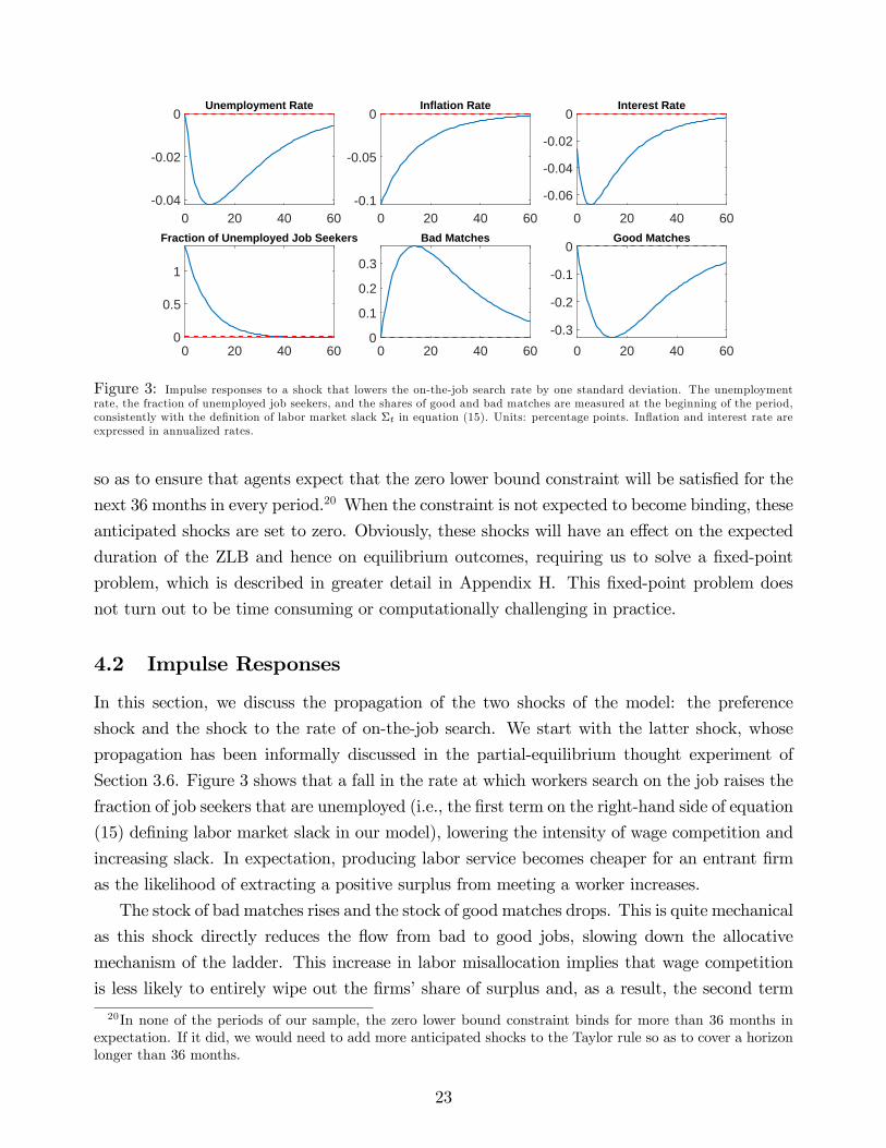
Figure 3: Impulse responses to a shock that lowers the on-the-job search rate by one standard deviation. The unemploymentrate, the fraction of unemployed job seekers, and the shares of good and bad matches are measured at the beginning of the period,consistently with the definition of labor market slack Σt in equation (15). Units: percentage points. Inflation and interest rate areexpressed in annualized rates.
so as to ensure that agents expect that the zero lower bound constraint will be satisfied for the
next 36 months in every period.20 When the constraint is not expected to become binding, these
anticipated shocks are set to zero. Obviously, these shocks will have an effect on the expected
duration of the ZLB and hence on equilibrium outcomes, requiring us to solve a fixed-point
problem, which is described in greater detail in Appendix H. This fixed-point problem does
not turn out to be time consuming or computationally challenging in practice.
4.2 Impulse Responses
In this section, we discuss the propagation of the two shocks of the model: the preference
shock and the shock to the rate of on-the-job search. We start with the latter shock, whose
propagation has been informally discussed in the partial-equilibrium thought experiment of
Section 3.6. Figure 3 shows that a fall in the rate at which workers search on the job raises the
fraction of job seekers that are unemployed (i.e., the first term on the right-hand side of equation
(15) defining labor market slack in our model), lowering the intensity of wage competition and
increasing slack. In expectation, producing labor service becomes cheaper for an entrant firm
as the likelihood of extracting a positive surplus from meeting a worker increases.
The stock of bad matches rises and the stock of good matches drops. This is quite mechanical
as this shock directly reduces the flow from bad to good jobs, slowing down the allocative
mechanism of the ladder. This increase in labor misallocation implies that wage competition
is less likely to entirely wipe out the firms’share of surplus and, as a result, the second term
20In none of the periods of our sample, the zero lower bound constraint binds for more than 36 months inexpectation. If it did, we would need to add more anticipated shocks to the Taylor rule so as to cover a horizonlonger than 36 months.
23
of the right-hand side of equation (15) rises, implying a further decline in the intensity of wage
competition among firms and a further increase in slack. As the likelihood of being engaged
in wage competition that will zero the surplus for entrant labor service firms falls, inflation
drops and the central bank cuts the interest rate, stimulating aggregate demand and reducing
unemployment. Moreover, attracted by the expectation of cheaper labor, more firms enter the
labor service sector, i.e., more vacancies are created, expanding aggregate supply, which also
contributes to lowering the unemployment rate.
Note that the fall in the unemployment rate, in isolation, contributes to lowering the prob-
ability for an entrant firm to meet an unemployed worker and hence causes wage competition
to become more intense. Yet, as shown in the lower left panel of Figure 3, it turns out that in
equilibrium this effect is dominated by the fall in the rate of on-the-job search, which operates
in the opposite direction, raising the fraction of unemployed job seekers.
By showing the response of the fraction of job seekers who are unemployed and that of the
stock of workers employed in bad matches, we want to provide a decomposition of our measure
of slack, Σt, defined in equation (15). While in the immediate aftermath of the shock, inflation
responds mostly to the rise in the fraction of unemployed job seekers, the persistent change in
the match composition of the employment pool weighs down on inflation later on, contributing
to keeping inflation below its long-run value for some time. Interestingly, a negative shock to
the rate of on-the-job search can generate simultaneously a persistent rise in output, together
with a fall in unemployment, inflation, and productivity. Incidentally, these patterns seem to
accord well with the dynamics that have characterized the U.S. economy in recent years.
A negative preference shock raises the unemployment rate and cyclical misallocation and
lowers inflation. Analogous to the case of the shock to the rate of on-the-job search, in the
immediate aftermath of a preference shock the dynamics of inflation reflect mostly the response
of the fraction of unemployed job seekers, which influences the intensity of interfirm wage
competition. But as the on-the-job search rate converges to its steady-state value, the effects
of labor misallocation on labor market slack takes over, raising the persistence of inflation after
the shock. We show the impulse responses of preference shocks and provide more details in
Appendix I.
4.3 The On-the-Job Search Rate in the Macro Data
We show that for a given value of bad and good matches at the beginning of our sample period
(i.e., in April 1990), observing the unemployment rate and the EE rate implies the entire time
series of the on-the-job search rate st, as well as the time series of bad matches l0b,t+1 and good
matches l0g,t+1. The exact identification of these variables comes from a set of model’s equations
and does not require solving the model. We first show this property of the model. Then we
use the observed series of the unemployment rate and the EE rate to actually recover the on-
24
the-job search rate and the share of bad matches. We use the equations linearized around the
steady-state equilibrium where ˜ denotes linearized variables.
The observed series of unemployment rates informs u0,t+1 and hence the aggregate unem-
ployment at the end of the period ut through the following equation
ut =u0,t+1
1− δ , (21)
which is is obtained by combining equations (3) and (4) and linearizing.
Endowed with the end-of-period unemployment rate ut, we can linearize equation (5) to pin
down the job finding rate φt at time t as follows:
φt =(1− φ) u0,t − ut
u0
, (22)
where u0 denotes the unemployment rate at the beginning of the period in steady state and φ
is the job finding rate in steady state. We iterate on equations (21) and (22) using the observed
series of the unemployment rate, which yields a time series for the job finding rate φt.
We then linearize the definition of the EE flow rate (EEt) in the model, which reads as
follows:
EEt ≡stφ (θt)
[l0b,t(ξbν + ξg
)+ l0g,tξgν
]l0b,t + l0g,t
. (23)
The EE rate is the ratio of how many workers employed at the beginning of the period have
switched jobs (the EE flows) to the total numbers of workers employed at the beginning of the
period. Consistently with our model, the EE flows are given by the sum of all the workers who
find a better match and the fraction ν of those workers who find an equally valuable match.
Linearizing equation (23) yields the following equation, which expresses the on-the-job search
rate st as a function of the observed EE flow rate EEt, the job finding rate φt, and a bunch
of variables that are predetermined at time t, such as the distribution of the quality of the
matches at the beginning of period t (l0b,t and l0g,t):
st =s
EEEEt −
s
φφt −
s
ν(l0b + l0g
) [sφ [(ξb + νξg)]
EE− 1
]l0b,t
− s
ν(l0b + l0g
) [sφξgEE
− 1
]l0g,t. (24)
Because l0b,t and l0g,t are predetermined at time t, this equation allows us to exactly measure the
on-the-job search rate st consistently with the series for the job finding rate φt and the observed
EE flow rate EEt.
With the rates φt and st at hand, we can use the observed unemployment rate u0,t to pin
25
down the fraction of bad and good matches in the next period t + 1, using the linearized laws
of motion for low- and high-quality matches in (18) and (19), which read as follows:
l0b,t+1 = − (1− δ){φξgl
0b st +
[sξgl
0b − ξbu0
]φt
}+ (1− δ)
{[1− sφξg
]l0b,t + φξbu0,t
}(25)
l0g,t+1 = (1− δ)[l0g,t + φξgl
0b st + sφξg l
0b,t + φξgu0,t +
[sξgl
0b + ξgu0
]φt
]. (26)
With the knowledge of the distribution of match quality at time t + 1, we can go back to
equation (24) and obtain the on-the-job search rate in period t + 1 (st+1). Repeating these
steps will give us the time series of the on-the-job-search rate st, as well as the time series for
the distribution of match quality in our sample. Note that this procedure allows us to also
obtain the series of labor market slack by using equation (15).
It is important to notice that solving the model is not needed to pin down exactly the series
of the on-the-job search rate. This property of the model allows us to estimate the parameters ρsand σs before solving the model. This procedure is conditioned on the fraction of bad matches
at the beginning of the sample period (in our case April 1990). We assume that the distribution
of match quality is at steady state at that point in time.21
One concern with this approach is that by relying entirely on the unemployment rate to
estimate the job finding rate in equations (21) and (22), we are not taking into account changes
in the separation rate or in the participation rate, potentially leading to biased estimate of the
job finding rate. This is a concern because this bias could distort our estimate of the on-the-job
search rate and of labor misallocation. A way to mitigate this problem is to directly use the job
finding rate measured in the data in place of the observed rate of unemployment and obtain
the series of the on-the-job search rate and those of the good and bad matches by iterating on
equations (24)—(26). At the same time, though, using job finding rates would bias the implied
unemployment rate, which is one of the three key drivers of inflation in the model. Our main
results are very little affected by using the job finding rate computed following Shimer (2005)
instead of the unemployment rate as an observable. The only noticeable difference is in the
estimated behavior of labor market slack over the Great Recession period, when the separation
rate spiked up in the data in a way that is not captured by the model. Because this effect is
moderate and contained within a handful of quarters, it does not materially affect our analysis
on the pre-Great Recession data, which will be shown in Section 5.
We use two monthly time series to measure the on-the-job search rate and the other labor
market variables. The first series is the civilian unemployment rate measured by the U.S.
Bureau of Labor Statistics (BLS). The second series is the EE flow rate measured by the
21The results would not change if we introduced a Gaussian prior reflecting uncertainty about the initialconditions and then used the Kalman filter to optimally estimate these initial conditions.
26
EE Rate
2000 20100.02
0.025
Bad Matches
2000 2010
0.3
0.35Good Matches
2000 20100.6
0.65
Unemployment Rate
2000 2010
5
10Job Finding Rate
2000 2010
0.2
0.4
Search Rate
2000 2010
0.2
0.3
0.4
Figure 4: Labor market variables simulated from the calibrated model using the shocks that allow the model to explain exactlythe observed unemployment rate and the employment-to-employment (EE) flow rate, which are shown in the left panels. The reddashed lines denote the model’s steady-state value of each simulated variable.
Current Population Survey (CPS). We correct this series as suggested by Fujita, Moscarini,
and Postel-Vinay (2019) and extend it back to April 1990 by splicing this series with the quit
rate measured by Davis, Faberman, and Haltiwanger (2012).22 While the main focus of the
paper is on the period that follows the Great Recession, which is when the standard theories of
inflation most significantly fail, we show the behavior of the rate of on-the-job search and our
measure of bad jobs over this longer period of time. We think that this exercise is interesting
given that, to our knowledge, this paper is the first one that measures the search rate and the
fraction of good and bad matches using aggregate labor market flows.
Figure 4 shows the dynamics of the rates of on-the-job search st and bad jobs l0b,t, along with
the two traditional labor market variables– the unemployment rate and the job finding rate
rate φt– over our sample period that goes from April 1990 through December 2018. The panels
on the left report the observable variables. The traditional measures of labor market slack,
such as the unemployment and the job finding rate, reported in the upper panels of Figure 4,
suggest that the U.S. labor market became quite tight in recent years; however, the dynamics
of two key drivers of the model’s labor market slack in equation (15), i.e., the on-the job-search
rate and the stock of bad matches, paint a different picture. After the Great Recession, the
rate of on-the-job search fell to a historically low level, and bad matches increased, remaining
at a high level throughout the recovery. This latter finding implies that cyclical misallocation
was still high, bearing down on inflation and labor productivity.
Quite interestingly, while the amount of good matches was chugging along well in recent
years and was close to its long-run value, the convergence of bad matches slowed down markedly.
22While the quit rate also includes workers who leave their jobs to become unemployed or to exit the laborforce, Elsby, Hobijn, and Sahin (2010) document that 86% of the workers observed quitting their jobs movedirectly to a new job.
27
This pattern suggests that the low unemployment rate led to the creation of a large number of
low-productivity jobs that would be converted to high-productivity jobs only slowly because of
the record low rate of on-the-job search.
The prediction that bad jobs were still heightened late in the sample period is consistent with
the Survey of Consumer Expectations, which shows that about 30% of the workers employed
in 2017– after eight years of recovery– were not fully satisfied with how their current job fit
their experience and skills.23 This increase in bad jobs also accords well with the findings in
Jaimovich et al. (2020), who show that a third of the workers who were employed in routinary
occupations before the Great Recession could not find similar jobs and remained stuck in
nonroutinary manual occupations.
Using the longer sample, we find the on-the-job search rate implied by the model and
reported in the top right corner of Figure 4 exhibits a clearly countercyclical pattern.24 This
countercyclicality is due to the higher volatility of the job finding rate relative to the EE rate.
Because the job finding rate enters with a minus sign in the measurement equation (24) and
is a strongly procyclical variable, the on-the-job search rate has to be countercyclical. Recall
the fractions of good matches l0g,t and bad matches l0b,t are predetermined at time t and hence
cannot adjust to explain the time-t changes in the job finding rate and the EE rate.
A number of explanations could support this countercyclical behavior of the on-the-job
search rate. The decision to look for jobs is likely to be positively related to individual income
risk, which is countercyclical. So it may be that on average, fewer employed workers search in
expansions simply because less of them feel at risk of losing their jobs. To the extent that this
behavior dampens the volatility of the EE rate in the data, our model rationalizes it with a
countercyclical rate of on-the-job search. But the countercyclicality of on-the-job search may
as well derive from compositional effects, which could also affect the dynamics of the EE flow
rate in the data. Workers may search harder and hence switch jobs more often when they
are employed in bad matches, whose number is generally big at the beginning of expansions.
This view is consistent with the findings in Faberman et al. (2019), who show that employed
workers search more intensively, the lower their residualized wage. In addition, workers who are
hired at the beginning of an expansion are generally more skilled and dynamic than those who
tend to find jobs when the labor market is already very tight. This view is consistent with the
findings in Cahuc, Postel-Vinay, and Robin (2006), who show that higher-skilled workers tend
to be more mobile than lower skilled ones. To the extent that these mechanisms influence the
behavior of the EE flow rate in the data, the model will predict the rate of on-the-job search to
be countercyclical. Taken together, all these explanations also suggest a possible reason why
23One of SCE questions reads as follows: "On a scale from 1 to 7, how well do you think this job fits yourexperience and skills?" About 30% of the respondents reported a satisfaction of 5 or less.24Kudlyak and Faberman (2019) observe the job application behavior of the users of Snag-A-Job, an online
job site, and find results that are consistent with the search intensity of the employed being countercyclical.
28
the search rate in Figure 4 had fallen to its historical trough by the end of the sample. The
very prolonged fall in the rate of on-the-job search might be related to the exceptionally long
expansion the U.S. economy was going through.
One can be concerned that we do not allow the probability of drawing a good match ξg to
vary over time. Allowing for it to do so would change our estimate of the on-the-job-search rate
as this probability enters the measurement equation (23). One problem with this approach is
that the large procyclicality of the job finding rate φt relatively to the EE flow rate EEt implies
that matches created in recessions are on average more productive, which is at odds with the
empirical evidence reviewed by Barlevy (2002). Imposing that the probability of drawing a
good match is countercyclical would reinforce our finding that the on-the-job search rate is
countercyclical.
4.4 Interfirm Wage Competition and Inflation
After having determined the in-sample dynamics of the model’s labor market variables, we are
in the position to validate our partial-equilibrium conjecture in Section 3.6, according to which
the measure of slack Σt, reflecting the intensity of interfirm wage competition, is an excellent
proxy for inflation in our general equilibrium model.
Equation (15) also characterizes the three components of the model’s labor market slack
Σt, which are the unemployment rate u0,t, the measure of bad matches (capturing the degree
of cyclical labor misallocation) l0b,t, and the share of workers searching on the job st. If the
conjecture made in Section 3.6 is correct, then a linear combination of these three components
is also key to determine the contemporaneous rate of inflation in the linearized model.
To verify this conjecture, we simulate the calibrated model for a large number of periods (one
million) and then regress the simulated (annualized) series of inflation on the three determinants
of slack defined in equation (15). This procedure gives us three weights that maximize the
explanatory power of the three components of labor market slack on inflation. The weights are
as follows:
πt = −0.1718[−0.1719,−0.1718]
u0,t − 0.0468[−0.0468, −0.0468]
l0b,t + 0.0419[0.0419, 0.0419]
st, (27)
for which we report the 95% confidence interval for the coeffi cient within square brackets under
the estimated value.
The R-squared of the ordinary least squares (OLS) regression is 0.9993, which signifies a
close-to-perfect ability of the three labor market variables to explain contemporaneous inflation
in the model. This confirms our conjecture that the measure of slack in equation (15), which
reflects the intensity of interfirm wage competition, is a key proxy of inflation in the model. This
result is not totally surprising given the thought experiment in Section 3.6 where we studied the
free-entry condition (12) in isolation, as well as the inspection of the impulse response functions
29
Inflation Rate
2012 2014 2016 2018
-1
-0.5
0
0.5Contrib of Shocks to Search RateContrib. of Preference ShocksModel Inflation (year-over-year rate)Data: Core PCE Inflation Gap
Contribution of the Three Drivers of Inflation
2012 2014 2016 2018
-0.6
-0.4
-0.2
0
0.2
0.4 Contrib. of UnemploymentContrib of MisallocationContrib. of Search RateModel Inflation (month-over-month rate)
Figure 5: Left panel: core PCE inflation gap in the data (red line with the star markers) and model’s corresponding inflation ratein deviation from its steady state value (blue solid line). The bars denote the contribution of the search rate shocks (black bars)and that of the preference shocks (white bars) to the model’s inflation. The core PCE inflation gap is obtained by subtracting theten-year PCE inflation expectations measured by the Survey of Professional Forecasters from the year-over-year core PCE inflationrate. The model’s inflation is also computed as the year-over-year inflation rate. All rates are in percent and annualized. Rightpanel: Month-over-month annualized model’s inflation rate (blue solid line) and the contributions of the three components of labormarket slack Σt to this rate (bars). We use the estimated equation (27) to quantify these contributions.
in the previous section. While the three components in the right-hand side of equation (27)
are not derived from a formal notion of output gap in the model, in practice, as we will show,
they allow for a decomposition of inflation that turns out to be very useful in interpreting the
results of the paper in the next section.
4.5 The Missing Inflation Puzzle Explained
We want to evaluate the ability of the model to explain the missing inflation during the recovery
that followed the Great Recession. We are particularly interested in this period because the
conventional theories of inflation more clearly fail to adequately account for the missing inflation,
as shown in Section 2. The data set is identical to the one used to measure the on-the-job search
rate in Section 4.3. We use our linearized model to retrieve the series of two shocks that make
the model explain exactly the observed unemployment rate and EE flow rate. We then feed
the model with these shocks to simulate the inflation rate predicted by the model in the last
decade.25
The left panel in Figure 5 illustrates the main results of the paper by comparing the inflation
rate in the data with the rate of inflation simulated from the model, as well as presenting its
shock decomposition. The red line with star markers denotes the observed core PCE inflation
gap, which is obtained by subtracting the ten-year PCE inflation expectations measured by
25As before, we assume that the economy is in steady state at the beginning of the sample period. Differentassumptions on the initial conditions would not affect our results because the sample period begins in April1990 and the analysis focuses on a briefer period that starts several years later (specifically, in January 2011).
30
the Survey of Professional Forecasters from the year-over-year core PCE inflation rate. The
blue solid line in the left panel denotes the corresponding measure of inflation predicted by the
model, using the simulation procedure described earlier. The black and white bars indicate the
contributions of the shocks to the search rate and to preferences, respectively. The bars should
be interpreted as the inflation rate predicted by the model when we feed it with each one of
these shocks.
Unlike the traditional measures of slack analyzed in Figure 2, our alternative measure of
slack reflecting the intensity of interfirm wage competition can explain the missing inflation of
the past decade. The fit of the high-frequency behavior of inflation cannot be perfect because
we use only two labor market variables in our empirical exercise. As illustrated by the black
bars, the missing inflation can be explained by the decline in the rate of on-the-job search.
This drop reduced the intensity of wage competition for employed workers throughout the
recovery, generating a fair amount of deflationary pressures, in spite of the steady decline in the
unemployment rate. The preference shocks, which are identified by the rate of unemployment,
capture the state of the business cycle and the effects of the ZLB constraint. The white bars in
the left panel of Figure 5 show that these factors contributed to generating deflationary pressures
in the immediate aftermath of the crisis and positive inflationary pressure over the latest years of
the sample when the labor market became very tight. Nevertheless, the deflationary pressures
due to the decline in the rate of on-the-job search (the black bars) more than compensated
for the inflationary pressures due to the preference shocks (the white bars) in latest years. In
accordance with the impulse responses shown in Section 4.2, the fall in the rate of on-the-
job search contributed to increasing production and to lower the rate of unemployment while
exerting downward pressure on the rate of inflation.
We now use the decomposition of inflation shown in equation (27) to provide further intuition
about which factors are contributing to the missing inflation. The right panel of Figure 5
visualizes the decomposition of the model’s annualized month-over-month inflation rate into
its three main drivers: the unemployment rate, the stock of bad jobs, and the on-the-job
search rate. At the beginning of the recovery, inflation was low primarily because of the record
surge in the unemployment rate during the Great Recession, as illustrated by the white bars.
After 2015, further improvements in aggregate labor market conditions quickly lowered the
share of unemployed job seekers, causing the unemployment rate to reverse the sign of its
contribution to inflation. However, in the same years, the on-the-job search rate declined
rapidly, putting downward pressures on inflation (the black bars) and dominating the effects of
the unemployment rate (the white bars).
The role played by the incidence of bad matches is also very interesting (the gray bars in
the right panel of Figure 5). Bad matches have always contributed to keeping inflation below
its long-run level. According to the model’s results, in the earlier part of the period of interest,
31
after the unusually severe recession, a large fraction of unemployed workers took a first step onto
the ladder, raising the stock of bad jobs. This development is consistent with the propagation
of preference shocks to the share of bad matches shown in Figure 12 in Appendix I and is fairly
typical in this class of models as it takes time, after a worker loses her job, to climb the ladder
all the way up again. Later in the recovery, as the on-the-job search rate declined sharply, the
speed at which workers moved to better jobs fell, exacerbating labor misallocation and keeping
the intensity of wage competition low. The gray bars clearly highlight the important role played
by the cyclical match composition of the employment pool in explaining the missing inflation.
What is So Special About the Great Recession? Figure 4 suggests that there may be
nothing special about the Great Recession, given that the countercyclicality of the on-the-job
search rate emerges with a striking empirical regularity. In putting upward pressure on inflation
in recessions and downward pressure on inflation in expansions, such countercyclicality of the
search rate helps explain the lack of serious deflationary and inflationary episodes in the U.S.
over the past thirty years. We mainly focus on the most recent expansion because this is the
period in which the traditional measures of labor market slack more spectacularly failed to
explain how inflation behaved, as shown in Section 2.
The Role of Labor Costs The central finding of this paper is that the shallow dynamics of
interfirm wage competition, which reflects the sluggish recovery of the observed EE flow rate
during the latest expansion, accounted for the missing inflation of the past decade. We now
look at two popular measures of firms’labor costs to verify that these costs did indeed remain
subdued throughout the post-Great Recession recovery. The left panel of Figure 6 compares
the 12-month moving average of the month-over-month growth rate of the nominal marginal
costs simulated from the calibrated model (blue solid line) with the 12-month moving average
of the month-over-month growth rate of U.S. average hourly earnings (black dashed line). The
horizontal red dashed line denotes the average wage growth in the data. The mean and the
volatility of the model’s implied growth rate of marginal costs are rescaled to match those in the
data. Rescaling the volatility of the model’s series facilitates the readability of the graph and
is neutral with respect to the in-sample correlation of the two plotted series, which is strikingly
high (0.60).
There are two takeaways from the left panel of Figure 6. First, we do not see an acceleration
in wage growth in recent years, in contrast to what would be implied by a standard wage Phillips
curve combined with the various measures of slack considered in Section 2. Second, our model
explains the lack of upward pressures on labor costs observed in the data with the decline
in the on-the-job search rate, which brought about a persistent fall in the intensity of wage
competition. Similar conclusions can be reached by looking at the right panel of Figure 6,
32
Labor Costs (AHE)
2008 2010 2012 2014 2016 2018
1.5
2
2.5
3
3.5
4
4.5modeldatamodel forecasts
Labor Costs (ECI)
2008 2010 2012 2014 2016 2018
1
1.5
2
2.5
3
modeldatamodel forecasts
Figure 6: Left panel: Nominal marginal costs growth rate in the model and the growth rate of the average hourly earnings (AHE)of all employees: total private (CES0500000003). Moving average over the last 12 months. Source: Bureau of Labor Statistics(BLS). Units: Percentage points of annualized rates. Frequency: monthly. Right panel: Nominal marginal costs growth rate inthe model and the growth rate of the Employment Cost Index (ECI): Wages and Salaries: Private Industry Workers (ECIWAG).Moving average over the last four quarters. Source: Bureau of Labor Statistics (BLS). Units: Percentage points of annualizedrates. Frequency: quarterly. The series of nominal marginal costs implied by the model are made quarterly by taking the averageof monthly growth rates of the nominal marginal costs. In both panels, the blue dotted-dashed line marks the model’s forecasts ofnominal marginal costs growth for the year 2019. The red horizontal dashed line denotes the long-run average of wage growth inthe data.
which compares the model’s predicted growth rate of nominal marginal costs with the growth
rate in the Employment Cost Index measured by the BLS.
Because our data set concludes at the end of 2018, we show the model’s forecasts for the
last 12 months of data (the blue dotted-dashed line in both panels of Figure 6). We include
the 2019 data on wage growth, showing that it stopped increasing. This sudden stop is diffi cult
for standard models to explain given that traditional measures of labor market slack suggest
the labor market was very hot in 2019. While wage growth was close to its long-run value (red
dashed line), in 2019 according to our model there were no significant wage pressures.
Endogenizing the On-the-Job Search Rate In this paper we treat the rate of on-the-
job search as an exogenous process. We believe that this is the right approach at this stage
given that a theory of what drives this rate has yet to emerge. It is important to notice that
the exact identification of the rate of on-the-job search implies that endogenizing the search
decision would not affect the in-sample estimation of this rate, which is shown in the upper
right panel of Figure 4. It follows that any theory used to microfound workers’decisions about
how frequently to search on the job can affect the inflation predicted by our model insofar as
these theories can influence agents’expectations about the future evolution of the rate.
In the model, agents form expectations about the likely evolution of the on-the-job search
rate by using an AR(1) process whose parameters (ρS and σS) are estimated via maximum
33
likelihood, as explained in Section 4.1.26 In Appendix G, we show that reasonable deviations
from the maximum likelihood estimates of the autocorrelation parameter, which could be war-
ranted by the microfoundation of the dynamics of the on-the-job search rate, do not materially
affect the model’s predicted path for inflation in the past decade.27 This result suggests that
endogenizing the decision to search on the job is unlikely to significantly affect our conclusions.
4.6 The On-the-Job Search Rate in the Micro Data
In the previous section, we illustrated that, according to our model, the main reason why
inflation has remained below target even late in our sample period is because the prolonged
fall in the rate of on-the-job search has lowered the intensity of interfirm wage competition. As
explained in Section 4.3, given the assumptions of the model, st is implied by the time series
of both the EE rate and unemployment rate.
In this section, we look into the micro data to see if our macro-based measurement of the
on-the-job search rate is validated at the micro level. To this end, we explore a new survey that
is informative about the search behavior of employed workers; it has been administered by the
Federal Reserve Bank of New York as a supplement to the Survey of Consumer Expectations.
The SCE is a monthly and nationally representative survey of about 1,300 individuals. This
survey is very useful for our purpose because it directly asks employed workers whether they
have been actively searching for work in the previous seven days.28 In this paper, we use SCE
data available from 2014 trough 2017. Even if this is admittedly a very limited period of time,
it still covers four years in which our model predicted that the on-the-job search rate was below
its long-run value and kept falling down.
Figure 7 plots the on-the-job search rate implied by the model, st, and the corresponding
measure in the micro data (blue solid line and the black dashed-dotted line, respectively). The
figure shows that the fall in the on-the-job search rate predicted by our model using aggregate
labor market flows is strikingly close to the one measured in the micro data.
When the model’s variable st is measured from equation (24), it effectively picks up a wedge
between EE and UE rates, which may as well confound other effects. For instance, while the
model abstracts from the intensive margin of on-the-job search, the fall in st measured from the
macro data could potentially reflect a decline in the average number of hours spent searching.
Alternatively, while the model assumes that conditional on searching, both unemployed and
26The AR(1) process is the best at fitting the model’s time series of the on-the-job search rate to the actualdata’s.27We do not perturb the standard deviation of the shocks to the on-the-job search rate σS , as doing so would
quite clearly have no effect whatsoever on expectations and hence on the model’s predicted path of inflation.28Question JS9 of the survey asks the following: "And within the LAST 7 DAYS, about how many TOTAL
hours did you spend on job search activities? Please round up to the nearest total number of hours." We dropself-employed workers when computing the on-the-job search rate from the SCE.
34
2014 2015 2016 2017
0.19
0.2
0.21
0.22
0.23
On-the-Job Search Rate
Model (Macro Data)Micro Data
Figure 7: The on-the-job search rate in the model and in the Survey of Consumer Expectations. In the Survey, the rate iscomputed by dividing the workers who have searched at least one hour within the last seven days by the total number of workerssurveyed. The rate is conditional on those surveyees who are working for someone else.
employed workers find jobs at the same rate φ (θt), it may well be that in the data the arrival
rate of job offers, conditional on searching, has diverged for these two types of job seekers,
with offers becoming less frequent for the employed workers relative to the unemployed. This
could be the case, for instance, if over time the employed workers had experienced a decline in
the availability of suitable jobs relative to the unemployed or just faced more stringent hiring
practices.
Using information on the hours of search for the employed workers in the SCE, we find that
the fall in the aggregate amount of time spent searching is entirely explained by the extensive
margin; that is, the effect is due to a fall in the incidence of job search among the employed–
and not to a decrease in the average number of hours dedicated to search. We also looked
at how the arrival rate of job offers for the employed workers varied over our sample period
relative to the arrival rate of offers for the unemployed. That is, we computed, both for the
employed and the unemployed, the ratio between the total number of offers received– and not
necessarily accepted– and the aggregate total number of hours spent searching. The ratio of
these two ratios does not exhibit a clear pattern. Therefore, the SCE validates the decline of
the on-the-job search rate predicted by our macro model, at least for the period in which micro
data are available.
Why has the rate of on-the-job search declined over the post Great-Recessionrecovery? Investigating the determinants of the search behavior of the employed workers–
an avenue of empirical labor research that has recently been revived by the availability of new
sources of information29– is outside the scope of this paper. However, we discuss a number of
29See Kudlyak and Faberman (2019), Faberman et al. (2019), and Abraham and Haltiwanger (2019).
35
potential explanations that are consistent with the pattern that we observe. In doing so, we
link our investigation to other developments in the literature.
One possibility, as discussed in Section 4.3, is that the rate of on-the-job search dropped and
remained particularly low simply because it is countercyclical and the expansion was going on
for an extraordinarily prolonged period of time. Alternatively, the decline in this rate in recent
years can be explained by the discouragement of those employed workers who experienced the
disappearance of suitable jobs. Jaimovich et al. (2020) show that a third of the workers that
were employed in routinary occupations before the Great Recession could not find similar jobs
and were stuck in nonroutinary manual occupations. Furthermore, Jaimovich and Siu (2018)
show that the incidence of job polarization is higher in recession. To the extent that learning
about one’s grimmer employment prospects takes time and may lead to discouragement, job
polarization is consistent with the fall in the on-the-job search rate in recoveries.
Job polarization has also implications for the low-frequency behavior of the on-the-job search
rate. While we find that the on-the-job search rate reached a record low in recent years, we
could not find any conclusive evidence to prove or disprove the existence of an active trend in
the behavior of the on-the-job search rate in the past thirty years, which is shown in the upper
right panel of Figure 4. Therefore, we did not introduce a trend in the process driving the
search rate. It can be shown that adding such a trend would greatly help our model explain the
persistent missing inflation of the past decade. In the model economy, if price setters interpret
the recent decline in the on-the-job search rate to be a secular phenomenon, they will expect
the intensity of interfirm wage competition to remain weak even in the very long run and hence
will be even more reluctant to raise their price.30
5 Empirical Performance in an Earlier Period
So far we have shown that the model laid out in Section 3 can overcome the failure of the
traditional measures of labor market slack to explain the behavior of inflation over the post-
Great Recession recovery. In this section, we discuss how well the proposed theory of inflation
fares at explaining inflation dynamics during an earlier period starting in April 1990, when our
data set starts. Specifically, we look at a sample period that precedes the years in which the
traditional theories of slack have clearly stopped working– that is, a period before the year
2013. (cf. Figure 2).
We find that the ability of our model to explain inflation dynamics is overall comparable
30Other stories that suggest that the fall in the on-the job search rate may be structural include Autor etal. (2020), who document an increase in the concentration of firms at the top of the productivity distribution.If this is the case, it may be that over time, workers were facing less opportunities to climb the ladder andhence ended up searching less frequently. Another empirical fact that can play a role in persistently loweringthe on-the-job search rate is the decline in interstate mobility (Kaplan and Schulhofer-Wohl 2017).
36
with that implied by the traditional measures of slack in this earlier period. We do so in the
simplest possible way, which is to compare how our measure of slack based on the intensity
of wage competition in equation (15) performs relative to other traditional theory-based ones,
using standard Phillips Curve regressions. That is, we estimate the equation
πt = β · slackt + εt, (28)
where πt is the eight-quarter moving average of the quarter-over-quarter core PCE inflation
rate (annualized and in percent) and in deviation from 2%, which is assumed to be the long-run
value for core PCE inflation.31 We use the moving average as we are not interested in fitting
the high-frequency swings in inflation. The variable slack represents different measures of labor
market slack: our own Σt, based on the intensity of wage competition, and each of the measures
considered in Section 2– that is, the labor share; a version of the labor share augmented to
account for search and matching frictions; the unemployment gap; and detrended total hours,
which is the key observable to inform the output gap in state-of-the-art DSGE models, such as
those in Christiano, Eichenbaum, and Evans (2005), Smets andWouters (2007), and Justiniano,
Primiceri, and Tambalotti (2010). After having estimated the Phillips curve (28) for the period
1990Q2 through 2018Q4, we compute the root mean squared error (RMSE) of the different
specifications over different subsamples.
All the measures of slacks deliver very similar fits of the inflation rate, attaining RMSEs
bunched in an interval of around two basis points of the annualized percentage inflation rate.
We conclude that our measure does a comparable job of delivering a fit of inflation during
this sample period as other popular measures of labor market slack do. When we look at the
most recent period (2013Q1—2018Q4), the intensity of wage competition outperforms the other
measures of slack by significant margins in line with the results discussed in Section 2.
6 Concluding Remarks
We showed that standard theories of inflation based on the New Keynesian Phillips curve fail
to explain why inflation has remained subdued throughout the post-Great Recession recovery.
We introduced a model with the job ladder in which the fraction of workers searching on the
job influences labor market slack by affecting the degree of interfirm wage competition to hire
employed workers. We found that the model explains the missing inflation of the past decade
with the fall in the rate of on-the-job search and the associated weakening of wage competition
among firms. Finally, we verified that when the on-the-job search rate is identified at micro
31We cannot use the Survey of Professional Forecasters’expectations of PCE inflation over the next ten yearsto compute the inflation gap as we did in our empirical analysis that focused on the last decade. The reason isthat this measure of long-term inflation expectations became available only since 2008.
37
levels using survey data, a similar fall in this rate was detected from 2014 through 2017.
Our paper opens avenues for future research on the appropriate stabilization policies in
the presence of interfirm competition for the employed. For instance, an important question
to explore is whether monetary policy, whose primary goal is to stabilize inflation, has any
significant effect on workers’willingness to search for a new job. While the empirical literature
has made important progress in understanding how monetary impulses affect labor supply
mobility, very little is known about the effectiveness of monetary stimuli in incentivizing workers
to search on the job.
References
Abraham, G. K., and C. J. Haltiwanger (2019): “How Tight is the Labor Market?,”
Federal reserve bank of chicago working paper.
Atkeson, A., and L. E. Ohanian (2001): “Are Phillips curves useful for forecasting infla-
tion?,”Federal Reserve Bank of Minneapolis Quarterly Review, 25(1), 2—11.
Autor, D., D. Dorn, L. F. Katz, C. Patterson, and J. V. Reenen (2020): “The
Fall of the Labor Share and the Rise of Superstar Firms,”Quarterly Journal of Economics,
forthcoming.
Ball, L., and S. Mazumder (2011): “Inflation Dynamics and the Great Recession,”Brook-
ings Papers on Economic Activity, 42(1 (Spring), 337—405.
Barlevy, G. (2002): “The Sullying Effect of Recessions,”Review of Economic Studies, 69(1),
65—96.
Bianchi, F., and L. Melosi (2017): “Escaping the Great Recession,”The American Eco-
nomic Review, 107(4), 1030—1058.
Cahuc, P., F. Postel-Vinay, and J.-M. Robin (2006): “Wage Bargaining with On-the-Job
Search: Theory and Evidence,”Econometrica, 74(2), 323—364.
Christiano, L., M. Eichenbaum, and C. Evans (2005): “Nominal Rigidities and the
Dynamic Effects of a Shock to Monetary Policy,”Journal of Political Economy, 113, 1—45.
Christiano, L. J., M. S. Eichenbaum, and M. Trabandt (2016): “Unemployment and
Business Cycles,”Econometrica, 84, 1523—1569.
Coibion, O., and Y. Gorodnichenko (2015): “Is the Phillips Curve Alive and Well after
All? Inflation Expectations and the Missing Disinflation,” American Economic Journal:
Macroeconomics, 7(1), 197—232.
Davis, S. J., R. J. Faberman, and J. Haltiwanger (2012): “Labor market flows in the
cross section and over time,”Journal of Monetary Economics, 59(1), 1 —18.
Del Negro, M., M. Lenza, G. E. Primiceri, and A. Tambalotti (2020): “What’s Up
with the Phillips Curve?,”Brookings Papers on Economic Activity.
38
Dotsey, M., and R. G. King (2005): “Implications of state-dependent pricing for dynamic
macroeconomic models,”Journal of Monetary Economics, 52(1), 213—242.
Elsby, M. W. L., B. Hobijn, and A. Sahin (2010): “The Labor Market in the Great
Recession,”Brookings Papers on Economic Activity, 41(1 (Spring), 1—69.
Faberman, R. J., A. I. Mueller, A. Sahin, and G. Topa (2017): “Job Search Behavior
among the Employed and Non-Employed,”IZA Discussion Papers 10960, Institute of Labor
Economics (IZA).
Fernald, J. G. (2016): “Reassessing Longer-Run U.S. Growth: How Low?,”Working Paper
2016-18, Federal Reserve Bank of San Francisco.
Fujita, S., G. Moscarini, and F. Postel-Vinay (2019): “Measuring Employer-to-
Lindé, J., and M. Trabandt (2018): “Resolving the Missing Deflation Puzzle,” mimeo,
Freie Universitat Berlin.
McLeay, M., and S. Tenreyro (2019): “Optimal Inflation and the Identification of the
Phillips Curve,” in NBER Macroeconomics Annual 2019, volume 34. National Bureau of
Economic Research, Inc.
Moscarini, G., and F. Postel-Vinay (2016): “Did the Job Ladder Fail after the Great
Recession?,”Journal of Labor Economics, 34(S1), 55—93.
(2018): “On the Job Search and Business Cycles,”Mimeo Yale U. and U. College
London.
(2019): “The Job Ladder: Inflation vs Reallocation,”Mimeo Yale U. and U. College
London.
Phillips, W. (1958): “The Relation Between Unemployment and the Rate of Change of Money
Wage Rates in the United Kingdom, 1861 - 1957,”Economica, 25(100), 293—299.
Postel-Vinay, F., and J.-M. Robin (2002): “Equilibrium Wage Dispersion with Worker
and Employer Heterogeneity,”Econometrica, 70(6), 2295—2350.
Ravenna, F., and C. E. Walsh (2008): “Vacancies, unemployment, and the Phillips curve,”
European Economic Review, 52(8), 1494—1521.
Shimer, R. (2005): “The Cyclical Behavior of Equilibrium Unemployment and Vacancies,”
The American Economic Review, 95(1), 25—49.
Silva, J. I., and M. Toledo (2009): “Labor Turnover Costs and the Cyclical Behavior of
Vacancies and Unemployment,”Macroeconomic Dynamics, 13(S1), 76—96.
Sims, C., and T. Zha (1998): “Bayesian Methods for Dynamic Multivariate Models,” Inter-
national Economic Review, 39(4), 949—68.
Smets, F., and R. Wouters (2007): “Shocks and Frictions in US Business Cycles: A
Bayesian DSGE Approach,”The American Economic Review, 97(3), 586—606.
Stock, J. H., and M. W. Watson (2007): “Why Has U.S. Inflation Become Harder to
Forecast?,”Journal of Money, Credit and Banking, 39(s1), 3—33.
Stock, J. H., and M. W. Watson (2008): “Phillips Curve Inflation Forecasts,”Working
Paper 14322, National Bureau of Economic Research.
(2019): “Slack and Cyclically Sensitive Inflation,”Working Paper 25987, National
Bureau of Economic Research.
40
Appendix (For Online Publication)
In Appendix A, we show the acceptance ratio in the data. We summarize how to construct
the measure of marginal costs in a standard NK model in Appendix B. Different calibrations
and specifications for the Phillips curve studied in Section 2 of the main text are introduced,
and their ability to account for the missing inflation after the Great Recession is evaluated in
Appendix C, which focuses on Phillips curves with a backward-looking component. In Appendix
D we describe how the data set to conduct the VAR analysis in Section 2 of the main text is
constructed. In Appendix E, we show that state-of-the-art dynamic general equilibrium models
have hard time explaining the missing inflation. We show how to work out equations (13)
and (14) in the main text, which provide an analytical characterization of the surpluses in the
model, in Appendix F. In Appendix G, we show the robustness of our main results by varying
two parameters that are hard to calibrate: the probability of meeting a worker that is a bad
match for the firm (ξb) and the probability that workers switch jobs if they receive an outside
offer that makes them indifferent (ν). We also show how the results change when varying the
persistence of the on-the-job search rate (ρs). Finally, in Appendix H, we show how we solve
the model with an occasionally binding zero lower bound for the nominal interest rate.
A Acceptance Ratio
Figure 8 shows the ratio of the employment-to-employment flow rate, corrected as suggested by
Fujita, Moscarini, and Postel-Vinay (2019), to the unemployment-to-employment flow rate.32
This plot shows that the acceptance ratio rapidly rose during the Great Recession. However,
the acceptance ratio steadily decreased during the recovery and eventually moved below its
pre-Great Recession average computed over the period from February 1996 through December
2007, which is denoted by the red dashed line.33
Moscarini and Postel-Vinay (2019) interpret this ratio as the acceptance ratio. In their
model, because the fraction of accepted offers is higher when more workers are employed in
low-productivity jobs, this ratio is a proxy for the degree of labor misallocation and is inversely
related to inflation in their model. When this ratio is low, few offers are accepted on average as
labor is perfectly allocated and, as result, marginal costs and inflation are high in their model.
In our model, a low acceptance ratio may be due to either a high degree of misallocation or a
low share of workers searching on the job. Therefore, this ratio is not always a good predictor
of labor misallocation and inflation in our model. A better predictor is the empirical measure32The correction proposed by Fujita, Moscarini, and Postel-Vinay (2019) ends up revising the employment-
to-employment rate upward in recent years, causing the fall of this ratio to be less rapid and dramatic duringthe post-Great Recession recovery than one would obtain by using the uncorrected CPS series for the EE flowrate.33The CPS data start in February 1996.
Figure 8: Acceptance Ratio. The ratio of the employment-to-employment flow rate to the unemployment-to-employment flowrate. Both rates are computed by taking the three-month moving average of the Current Population Survey (CPS) flow data. The reddashed line denotes the mean of the ratio computed from February 1996 through December 2007. The employment-to-employmentrate is corrected as proposed by Fujita, Moscarini, and Postel-Vinay (2019).
of labor market slack, which is based on the intensity of interfirm wage competition, introduced
in Section 3.6.
B Computation of Real Marginal Costs in a Standard
New Keynesian Model with Search and Matching
We follow the work by Krause, Lopez-Salido, and Lubik (2008), who study the behavior of real
marginal costs in a simple New Keynesian model with search and matching frictions in the
labor market. Equation (32) from Krause, Lopez-Salido, and Lubik (2008, p. 898) defines the
real marginal cost as:
mct =Wt
α(ytnt
) +c′ (vt) /q (θt)− (1− ρ)Etβt+1c
′ (vt+1) /q (θt+1)
α(ytnt
) , (29)
where Wt denotes the real hourly wage, yt/nt is the average product of labor, c′ (vt) is the
derivative of the vacancy cost function with respect to vacancies, q (θt) is the vacancy filling rate,
βt+1 is the discount factor, and α is the elasticity of output to employment in the production
function. The first component on the right-hand side of equation (29) is the unit labor cost,
i.e., the ratio of the labor cost and the marginal product of labor. The second component stems
from the existence of search and matching frictions and can be interpreted as cost savings from
not having to hire in the following period.
Let st ≡ Wt/α(ytnt
)denote the unit labor cost, which equals the labor share of income
42
2009 2010 2011 2012 2013 2014 2015 2016 2017
=0.005
-6
-4
-2
0
2
4
6
8
Inflation Implied by the Traditional Measures of Slack
Unemployment GapLabor ShareLabor Market FrictionsData: Core PCE Inflation Gap
2009 2010 2011 2012 2013 2014 2015 2016 2017
=0.0005
-1.2
-1
-0.8
-0.6
-0.4
-0.2
0
0.2
0.4
0.6
0.8
Inflation Implied by the Traditional Measures of Slack
Unemployment GapLabor ShareLabor Market FrictionsData: Core PCE Inflation Gap
Figure 9: PCE refers to the Price Index for Personal Consumption Expenditures. The figure shows the inflation dynamics from2009Q1 through 2017Q3 using three traditional theories of inflation using a slope of the inertial Phillips curve of 0.005 (left panel)and 0.0005 (right panel) and the core PCE inflation gap. The assumed degree of inertia is equal to 0.90.
divided by the elasticity of output to employment. Krause, Lopez-Salido, and Lubik (2008)
show that linearizing equation (29) and rearranging leads to the following expression:
mct = st +1− φ1− β
[ξ
1− ξ
(ht − βEtht+1
)+ (εc − 1)
(vt − βEtvt+1
)− βEtβt+1 −
(1− β
)wt
],
(30)
where a hat variable is used to denote log deviations from the steady-state, ht denotes the job
finding rate, β is a discount factor adjusted for the rate of job separation, εc is the elasticity
of vacancy costs to vacancies, ξ is the elasticity of the matching function with respect to
unemployment, and φ = s/mc is the share of unit labor cost over total marginal costs. We
follow the calibration in Krause, Lopez-Salido, and Lubik (2008) and assume that ξ = 0.5,
1− φ = 0.05, and β = 0.943. In line with the model specified in Section 3, we assume a linear
vacancy cost function, which implies εc = 1, and log utility in consumption.
C Traditional Measure of Slack: Robustness
The most popular Phillips curve used in empirical studies features a backward-looking term:
πt = ιπt−1 + κϕt + Eπt+1, (31)
where the parameter ι reflects the degree of price indexation. We redo the same VAR-based
exercise as the one in Section 2 to evaluate the robustness of these results to the introduction
of price indexation and of a flatter Phillips curve. We kick off by setting the degree of price
indexation ιp to 0.9– an upper bound for plausible degrees of inertia. We consider two cases.
In the first case, we assume that the slope of the Phillips curve is κ = 0.005, as in the baseline
43
case analyzed in the main text. In the second case, we consider a very flat Phillips curve with a
parameter κ = 0.0005. While the first case allows us to evaluate how much adding a backward-
looking component alters the result shown in the main text (Figure 2), the second case is useful
to illustrate that even a very flat Phillips curve with a lot of price indexation cannot solve the
missing inflation puzzle.
The results are shown in Figure 9. In the left panel we show the first case, which confirms
that adding price indexation just makes the drop in inflation in 2009 more pronounced and
delayed. According to the traditional measures of slack, inflation should have picked up by
2014; only the unemployment gap predicts inflation staying below its long-run level until the
end of 2015. None of the measures explains why inflation has not risen after nine years of
economic expansion, even after introducing a very large degree of price indexation.
In the right panel of Figure 9 we show the second case, which combines a large degree of
price indexation with an extremely flat slope of the Phillips curve. Comparing the plots of the
left and right panels of Figure 9 reveals that a reduction of the slope in the presence of high
indexation decreases the predicted fall in inflation at the beginning of the sample and contains
the predicted rise in inflation at the end of the sample. Therefore, we conclude that a flatter
Phillips curve in and of itself does not solve the puzzle of the persistently low inflation observed
in the past decade. This is the case even if one endows the Phillips curve with a very large
price inertia.
D Construction of the Time Series and Their Sources
The time series used for the VAR analysis have been constructed from the following data
downloaded from the St. Louis Fed’s database called Federal Reserve Economic Data (FRED).
The labor share of income is computed as the ratio of total compensation in the nonfarm
business sector divided by nominal nonfarm GDP. In turn, total compensation is computed as
the product of compensation per hour (COMPNFB) times total hours (HOANBS), and nominal
GDP is the product of real output (OUTNFB) times the appropriate deflator (IPDNBS). All
series are quarterly and seasonally adjusted. We compute the deviations of the labor share from
its trend by computing log deviations from an eight-year moving average.
We follow Shimer (2005) and compute the job finding rate as φt = 1 −(ut+1 − ust+1
)/ut,
where ust+1 denotes the number of workers employed for less than five weeks in month t + 1
(UEMPLT5). The total number of workers unemployed in each month is computed as the
sum of the number of civilians unemployed less than five weeks (UEMPLT5), for 5 to 14
weeks (UEMP5TO14), 15 to 26 weeks (UEMP15T26), and 27 weeks and over (UEMP27OV).
The primary data are constructed by the U.S. Bureau of Labor Statistics from the CPS and
seasonally adjusted. To obtain quarterly percentage point deviations of the job finding rate
44
The Inflation Gap
2010 2012 2014 2016 2018
-2
-1.5
-1
-0.5
0
Smets and Wouters Model (Hours) Data (Core PCE Inflation Gap)
The Labor Market Gap
2010 2012 2014 2016 2018-8
-6
-4
-2
0
2
Figure 10: Left panel: PCE refers to the Price Index for Personal Consumption Expenditures. The black solid line: Inflationpredicted by the model of Smets and Wouters (2007) conditional on observing the series of hours plotted on the right panel. Theblue starred line: the difference between the annualized quarter-to-quarter core PCE inflation rate and the ten-year-ahead core PCEinflation expectations based on the Survey of Professional Forecasters. Right panel: Hours worked detrended using their eight-yearmoving average.
from its trend, we average monthly data over each quarter and then subtract the actual job
finding rate from its eight-year moving average.
We also use data on real gross domestic product (GDPC1), real gross private domestic
investment (GDPIC1), and real personal consumption expenditures (PCECC96). All data are
quarterly and seasonally adjusted. When computing percentage deviations of each of these
times series from its trend, we first remove a quadratic trend from the variable in logs and then
take the difference from its eight-year moving averages. To compute percentage deviations of
real wages from the trend we first remove a linear trend to the log of compensation per hour
(COMPNFB) and then take the difference with respect to its eight-year moving average.
We measure aggregate price inflation by taking log differences on the previous quarter of
the seasonally adjusted Consumer Price Index for All Urban Consumers (CPIAUCSL). We also
use quarterly data on the effective federal funds rate (FFR) and on the short-term natural rate
of unemployment (NROUST). We compute percentage point deviations of inflation, the federal
funds rate, and the natural rate of unemployment from trend as the difference from each series’
eight-year moving average.
E A State-of-the-Art Dynamic General EquilibriumModel
(Smets and Wouters 2007)
In this appendix, we evaluate the ability of a leading empirical general equilibrium model to
reconcile labor market and inflation dynamics in the post-Great Recession recovery. We use
45
the popular model introduced by Smets and Wouters (2007) to perform this exercise. This is
a model with many real and nominal frictions and a large array of shocks and is well known
to fit the U.S. macro series well. Smets and Wouters conduct a Bayesian estimation of the
parameters of their model using seven observables: consumption growth, investment growth,
GDP growth, hours (detrended for the labor force participation), inflation, real wage, and the
federal funds rate. Their sample period goes from 1966Q1 through 2004Q4. We extend their
data set trough 2018Q4 and detrend the series of hours using a eight-year moving average. We
make the latter change because the series of hours exhibited a significant downward shift since
the onset of the Great Recession and has never attained its pre-recession level again.
We use the extended data set to estimate the model. Then the same data set is used
to filter the state variables of the estimated model from the first quarter of 1966 through
the fourth quarter of 2008. For the subsequent periods (2009Q1—2018Q4), we filter the state
variables of the estimated model using only the series of hours in order to obtain inflation
predictions conditional on labor market data only. Recall that the emphasis of this paper is on
the apparently waning link between the labor market and inflation. The black solid line in the
right panel of Figure 10 shows the series of hours detrended using a eight-year moving average,
which we use to simulate the Smets and Wouters model.
Based on the series of hours, the Smets and Wouters’model predicts that inflation is above
target already in 2012. See the black solid line in the left panel of Figure 10. The plot also
reports the inflation gap in the data (blue starred line), which is computed by taking the
difference between the annualized quarter-to-quarter core PCE inflation rate and the ten-year-
ahead core PCE inflation expectations based on the Survey of Professional Forecasters. The
inflation gap in the data remains persistently below zero, whereas the Smets and Wouters’
model predicts that inflation moves above its long-run level as early as in 2012. Indeed, the
right panel of Figure 10 shows that the series of hours implied that the labor market became
tight (positive labor market gap) in 2015.
F Job Values and Sequential Auctions
In this section we derive the expressions for the surplus function St (y) in equation (13), following
the approach in Moscarini and Postel-Vinay (2019). We start by characterizing the value
functions for the states of employment and unemployment. The value of unemployment to a
worker j measured after worker reallocation has taken place and expressed in utility units is
determined as follows::
λtVju,t = b+βEtφ (θt+1)λt+1
[V je,t+1
(wt+1 (j) , yt+1 (j) | e0
t+1 = 0)]
+βEt (1− φ (θt+1))λt+1Vju,t+1,
(32)
46
where we let the indicator function e0t+1 = {0, 1} denote the state of employment at the begin-
ning of period t+ 1, before reallocation takes place.
The value to a worker j of being employed at the production stage of period t in a job of
productivity yt at wage wt after reallocation has taken place, but before the realization of the
current-period separation shock, is determined as follows:
λtVje,t (wt (j) , yt (j)) = λt
wt (j)
Pt+ βEtλt+1
{δ [1− φ (θt+1)]V j
u,t+1
+δφ (θt+1)V je,t+1
(wt+1 (j) , yt+1 (j) | e0
t+1 = 0)
+ (1− δ)V je,t+1
(wt+1 (j) , yt+1 (j) | wt (j) , yt (j) , e0
t+1 = 1)}. (33)
The above expression implies that the worker receives a wage wt(j)Pt
in exchange for her labor
services, plus a continuation value, which depends on whether the worker separates or not at the
end of the period. If separation occurs at rate δ, the worker will still be in the state of unemploy-
ment by the end of period t+1 if no job is found, which occurs with probability 1−φ (θt+1). In
this case the worker receives the expected present value EtVju,t+1. If instead the newly separated
worker finds a job in period t+1 with probability φ (θt+1), she gets the payoffof being in a match
of productivity yt+1 (j), paying the wage wt+1 (j), which is conditional on the worker having
separated at the end of time t and therefore being unemployed at the beginning of t + 1. The
expected present discounted value of a such job, expressed in units of the numeraire good is de-
noted by EtVe,t+1
[wt+1 (j) , yt+1 (j) | e0
t+1 = 0].With probability 1− δ instead, the worker does
not separate at the end of time t, receiving EtVe,t+1
[wt+1 (j) , yt+1 (j) | wt (j) , yt (j) , e0
t+1 = 1]
at the end of the next period. This expression captures the value of being employed at the end
of time t + 1 in a match with productivity yt+1 at the wage wt+1, conditional on having been
employed in a match with productivity yt (j) and wage wt (j) in the previous period and not
having separated between periods, i.e., being in employment at the beginning of period t + 1.
Note that this expected value includes the possibility of a job-to-job transition in period t+ 1.
We assume that firms have all the bargaining power, and hence, the unemployed workers
who take up a new offer are indifferent between being employed or unemployed, i.e.,
λtVe,t(wt (j) , yt (j) | e0
t = 0)
= b+ βEtλt+1Vju,t+1 (34)
independently of yt (j). It follows that
V ju,t =
b
λt+ βEt
λt+1
λtV ju,t+1 = Vu,t. (35)
Let V ∗e,t (y) denote the value to the worker of being employed under full extraction of a
firm’s willingness to pay at the end of time t. In this case a worker of productivity y receives
47
the maximum value that the firm is willing to promise in period t, including the payment of
the current-period wage. Let {w∗s (y)}∞s=t denote the state-contingent contract that deliversV ∗e,t(y) ≡ Ve,t (w∗t , y) . By promising to pay the contract {w∗s (y)}∞s=t, the firm breaks even in
expectation, that is, the expected present value of future profits is zero.
Now consider a firm that is currently employing a worker with productivity y under any
promised contract {ws (y)}∞s=t. Assume that the worker is poached by a firm with match
productivity y′. The outcome of the auction must be one of the following three:
1. V ∗e,t (y′) < Ve,t (wt, y); in this case the willingness to pay of the poaching firm is less than
the value of the contract that the worker is currently receiving. As a result, the incumbent
firm retains the worker with the same wage contract with value Ve,t (wt, y).
2. Ve,t (wt, y) ≤ V ∗e,t (y′) < V ∗e.t (y); in this case the willingness to pay of the poaching firm
is greater or equal to the value of the contract the worker is receiving in his current job,
but lower than the willingness to pay of the incumbent firm. The two firms engage in
Bertrand competition, and as a result, the incumbent firm retains the worker offering the
new contract V ∗e,t (y′).
3. V ∗e,t (y) ≤ V ∗e,t (y′); in this case the poaching firm has a willingness to pay that is no less
than the incumbent’s. If this condition holds with strict inequality, the current match
is terminated and the worker is poached at the maximum value of the contract that
the incumbent is willing to pay. If instead the worker is poached by a firm with equal
productivity, it is assumed that job switching takes place with probability ν. In either
case, the continuation value of the contract obtained by the worker is V ∗e,t (y).
The bargaining protocol above, together with the assumption that entrant firms make zero
profits in expectations, yields the free entry-condition, i.e., equation (12) in the main text,
which we display again below for convenience:
cf +c
$t
=u0,t
u0,t + st (1− u0,t)
{ξbSt (yb) + ξgSt (yg)
}(36)
+st (1− u0,t)
u0,t + st (1− u0,t)
{ξg
l0b,t1− u0,t
[St (yg)− St (yb)]
}.
Substituting out for the surplus functions in the above equations requires some steps. Start
by considering the case of a firm that has promised to pay the contract {w∗s (y)}∞s=t, which impliesthat the firm breaks even in expectation and is not able to promise higher wage payments in
case it enters an auction with a poaching firm. In this case, if no outside offers arrive the
worker receives a continuation value of V ∗e,t (y) from the incumbent firm. Otherwise the worker
is poached and, in accordance with point (3) above, receives from the new firm a contract
48
that is also worth Ve,t (w′, y′) = V ∗e,t (y). So either way, the worker receives a contract of value
V ∗e,t (y). The value to a worker of being employed under the contract {w∗s (y)}∞s=t can thereforebe written as:
V ∗e,t (y) = ϕty + βEtλt+1
λt
[δVu,t + (1− δ)V ∗e,t+1 (y)
], (37)
where ϕty is the marginal revenue product of selling y units of the service to the price setters.
Subtracting (35) from the above equation yields:
V ∗e,t (y)− Vu,t = ϕty −b
λt+ (1− δ) βEt
λt+1
λt
[V ∗e,t+1 (y)− Vu,t+1
]. (38)
Notice that the value to the worker of extracting all the rents associated with a type-y match,
V ∗e,t (y) − Vu,t, is in fact simply the surplus St (y). Iterating forward on the above expression,
we can define the surplus of a match with productivity y as:
St (y) = Et
[ ∞∑τ=0
(1− δ)τ(λt+τλt
ϕt+τy −b
λt
)]. (39)
Notice that the surplus function above is affi ne increasing in y, which implies that firms with
higher productivity win the auction and, therefore, workers cannot move to jobs with lower
productivity. For convenience, we can rearrange the above expression as
St (y) = yWt −bλ−1
t
1− β (1− δ) , (40)
where
Wt = ϕt + β (1− δ)Etλt+1
λtWt+1. (41)
Seen from the point of view of a service sector firm, Wt can be interpreted as the expected
present discounted value of the entire stream of current and future real marginal revenues
derived from selling one unit of the service until separation. From the point of view of a price
setting firm, which purchases labor services, Wt can be interpreted as the expected present
discounted value of the cost of purchasing one unit of the labor service by a firm until separation.
Using equation (40) we can now substitute for the surplus functions and rearrange to rewrite
the free-entry condition (12) as:
cf +c
$t
=u0,t
u0,t + st (1− u0,t)
[Wt
(ξbyb + ξgyg
)− bλ−1
t
1− β (1− δ)
](42)
+st
u0,t + st (1− u0,t)ξgl
0b,tWt (yg − yb) .
49
Sensitivity to b
2012 2014 2016 2018
-1
-0.8
-0.6
-0.4
-0.2
0
Infla
tion
Sensitivity to b
Calibrated ModelData
Sensitivity to
2012 2014 2016 2018
-1
-0.8
-0.6
-0.4
-0.2
0
Infla
tion
Sensitivity to Calibrated ModelData
Sensitivity to s
2012 2014 2016 2018
-1
-0.8
-0.6
-0.4
-0.2
0
Infla
tion
Sensitivity to s
Calibrated ModelData
Figure 11: Robustness. Left panel: The shaded area show the sensitivity of the model’s predicted year-over-year inflation rate tochanges in the probability that the meeting between the worker and the firm generates a bad match (ξb). The blue solid line denotesthe model’s predicted year-over-year inflation rate for our baseline calibration shown in Table 1. The red starred line denotes theyear-over-year inflation rate in the data (core inflation according to the Price Index for Personal Consumption Expenditures, orPCE) in deviations from the Survey of Professional Forecasters’PCE inflation expectations over the next ten years. The middleand right panels show the same plot when we perturb the probability that workers accept an offer if they are indifferent (ν) andthe persistence of the on-the-job search rate (ρs).
G Robustness
The shaded area in the panels of Figure 11 shows how the model’s prediction of inflation changes
as we vary the probability of meeting a worker that is a bad match for the firm ξb (left), the
probability that workers switch jobs if they receive an outside offer that makes them indifferent
(ν) (middle), or the persistence of the on-the-job search rate (ρs) (right). We consider values
of the parameter ξb ranging from 0.6 through 0.8, values of the parameter ν ranging from
0.25 through 0.75, and values of the parameter ρs ranging from 0 through 0.97 (the highest
confidence bound when the AR parameter of the series of the-on-the-job search st is estimated
by OLS). The blue solid line and the red starred lines denote the model’s predicted inflation rate
and the core PCE inflation gap for the baseline calibration reported in Table 1, respectively.
These lines are the same as the ones plotted in the left panel of Figure 5.
H Solving the Model with the ZLB Constraint
After being solved, our linearized model with the occasionally binding ZLB constraint in equa-
tion (20) can be represented in state-space form as follows:
st = Γ0st−1 + Γ1ε1t + Γ2ε
2t (43)
where the first k+1 rows of st contain the current policy rate and the expectations of the policy
rate in quarter t+ 1, ..., t+k. The model’s structural shocks are contained in ε2t . This vector of
50
shocks includes the preference shock and the shocks to the on-the-job search rate. The linear
system above also features a vector of dummy shocks ε1t . These shocks in ε
1t are appended to
the Taylor rule so that the constrained Taylor rule in equation (20) can be written as
Rt
R∗=
(Rt−1
R∗
)ρr [(Πt
Π∗
)φπ (Qt
Q∗
)φy]1−ρr
+
k∑j=0
ηjt−j, (44)
where ηjt are k+1 monetary shocks that are known by agents at time t and will hit the economy
at time t+j. These shocks belong to the vector ε1t in equation (43). These dummy shocks serve
the sole purpose of enforcing the ZLB constraint (i.e., prevent agents from expecting negative
nominal interest rates in any state of the world). Thus, the realizations of these dummy shocks
will be equal to zero in every states of the world in which the current and expected nominal
interest rates do not violate the ZLB constraint. It should be noted that the matrix Γ1 is a
matrix with k + 1 columns.
As explained in the main text, the shocks are obtained by inverting the 2× 2 square matrix
ZΓ2, where the matrix Z is a 2 × 2 observation matrix such that Yt = Zst with the vector Ytincluding the observables (i.e., the unemployment rate and the EE flow rate) used in the empir-
ical exercise whose results are described in Section 4.3 and Section 4.5. Under the assumption
that the matrix ZΓ2 is invertible (as it is in our case), this inversion allows us to retrieve the
sequence of shocks ε2t that identically explains the observed rate of unemployment and the EE
rate.
We start by setting t = 1, which denotes the first period of our sample Yt, and go through
the following steps:
1. Given the realization of the two shocks ε2t at time t, we set the matrix Ψ (0) = 0k+1×k+1,
ε1t (0) = 0k+1×1, i = 0, and go to Step 2.
2. Define the vector of adjustments to forward guidance shocks ∆ε1t that ensures the current
and/or the expected path of the future interest rates will respect the ZLB as follows:
∆ε1t =
(Γ
(0:k)1
)−1 [− lnR∗ − Γ
(0:k)0 st−1 − Γ
(0:k)1 (i) ·Ψ (i) ε1
t (i)− Γ(0:k)2 ε2
t
], (45)
where Γ(0:k)1 denotes the square submatrix made of the first k + 1 rows of the matrix Γ1.
With ∆ε1t at hand, we update ε
1t (i+ 1) = ε1
t (i) + ∆ε1t . Note that if the ZLB constraint
is not binding at time t, ∆ε1t = 0k+1×1.
3. Check if the below inequality is satisfied (the ZLB is not binding),
Γ(0:k)0 st−1 + Γ
(0:k)1 ·Ψ (i) ε1
t (i+ 1) + Γ(0:k)2 ε2
t > − lnR∗. (46)
51
0 20 40 600
0.1
0.2
0.3Unemployment Rate
0 20 40 60
-0.04
-0.02
0Inflation Rate
0 20 40 60-0.3
-0.2
-0.1
0Interest Rate
0 20 40 600
0.2
0.4
0.6
0.8Fraction of Unemployed Job Seekers
0 20 40 60
-0.05
0
0.05
Bad Matches
0 20 40 60
-0.2
-0.1
0Good Matches
Figure 12: Impulse responses to a negative preference shock by one standard deviation. The unemployment rate, the fractionof unemployed job seekers, and the shares of good and bad matches are measured at the beginning of the period, consistently withthe definition of labor market slack Σt in equation (15). Units: percentage points. Inflation and interest rate are expressed inannualized rates.
We adjust the diagonal matrix of zeros and ones, Ψ (i+ 1), so that the set of horizons
at which the ZLB is binding is characterized with a value equal to one in this matrix. If
Ψ (i+ 1) ε1t (i+ 1) 6= Ψ (i) ε1
t (i), set i = i + 1 and go to Step 2, or else the fixed point is
found and we set ε1t = Ψ (i+ 1) ε1
t (i+ 1) and go to Step 4.
4. Compute the next period’s state vector as follows:
st = Γ0st−1 + Γ1ε1t (i+ 1) + Γ2ε
2t . (47)
Set t = t+ 1, and go back to Step 1.
The st coming from equation (47) is the vector containing the model-predicted values of the
state variables, which is used to generate all the empirical results of the paper.
I Propagation of Preference Shocks
Figure 12 shows the responses to a negative preference shock. As done in the main text, we
report the responses of the labor market variables (unemployment, bad matches, and good
matches) at the beginning of the period, and as such they do not respond on impact by con-
struction. When the preference shock hits, households want to save more and consume less. As
a result, households’demand for the differentiated goods falls, leading to a drop in the price
setters’demand for the labor service and hence in its relative price ϕt. Forward-looking price
setters anticipate that marginal costs will remain low and cut their price, leading the inflation
rate to fall. Concurrently, the weakening of the price setters’demand for labor service reduces
52
entry in the labor market, which in turn induces unemployment to rise over the subsequent
periods. As the fraction of unemployed job seekers surges, labor becomes cheaper in expecta-
tion for an entrant service firm, because it is now more likely to extract a nonzero surplus from
the match. As a result, equation (15) implies an increase in labor market slack, along with a
decrease in the price of labor service, and, therefore, an even further drop in inflation in the
second period.
Also note that the stock of bad matches falls initially and then rises as the entry of more
labor service firms allows unemployed workers to find jobs and thus climb the ladder anew.
This rise in bad matches, along with the fall in good matches, further contributes to keeping
labor cheap for longer and to depressing price dynamics. Our measure of slack captures these
effects through the second term on the right-hand side of equation (15).
53
W O R K I N G P A P ER — DA N M A R K S N A T I O NA L B A N K