Discussion Paper 134

Institute for Empirical MacroeconomicsFederal Reserve Bank of Minneapolis90 Hennepin AvenueMinneapolis, Minnesota 55480-0291

March 2000

Bad Politicians

Francesco Caselli*

University of Chicago,Harvard University,and C.E.P.R.

Massimo Morelli*

Iowa State Universityand University of Minnesota

ABSTRACT

We present a simple theory of the quality of elected officials. Quality has (at least) two dimensions:competence and honesty. Voters prefer competent and honest policymakers, so high-quality citizens havea greater chance of being elected to office. But low-quality citizens have a “comparative advantage” inpursuing elective office, because their market wages are lower than the market wages of high-quality citi-zens (competence), and/or because they reap higher returns from holding office (honesty). In the politicalequilibrium, the average quality of the elected body depends on the structure of rewards from holdingpublic office. Under the assumption that the rewards from office are increasing in the average quality ofoffice holders there can be multiple equilibria in quality. Under the assumption that incumbent policy-makers set the rewards for future policymakers there can be path dependence in quality.

*We thank Alberto Alesina, Jim Alt, Scott Ashworth, Abhijit Banerjee, Marco Bassetto, Jeff Campbell, Harold Cole,Rafael Di Tella, Sven Feldmann, Giunia Gatta, Joao Gomes, Catherine Hafer, Pat Kehoe, Michael Kremer, LaurentLedoux, Rebecca Morton, Casey Mulligan, Ken Shepsle, Michele Tertilt, Mariano Tommasi and Alwyn Young forcomments. Caselli thanks the University of Chicago Graduate School of Business for support and the Federal Re-serve Bank of Minneapolis for hospitality. Morelli thanks the University of Minnesota for hospitality. E-mail:caselli@fas.harvard.edu; morelli@atlas.socsci.umn.edu. The views expressed herein are those of the authors andnot necessarily those of the Federal Reserve Bank of Minneapolis or the Federal Reserve System.

The truth is that the city where those who rule are least eager to do so will

be the best governed.

Plato.

1 Introduction

In democratic countries crucial economic-policy decisions are taken by elected officials, either

directly, or indirectly through the appointment of top civil servants. The quality of the

political elite can therefore have important repercussions on a countrys welfare. This paper

presents a simple theory of the quality of elected office holders.

There are at least two distinct and possibly uncorrelated dimensions to politicians

quality: competence and honesty. By competence we mean skilfulness at identifying the ap-

propriate economic-policy objectives and achieving them at minimum costs for taxpayers. To

make this notion concrete we will model competence as the ability to provide an indispens-

able public good with minimum tax revenues. We think competence in this sense is clearly

desirable, and in our model voters prefer competent over incompetent office holders.1 The

lack of honesty manifests itself in the harassment of private citizens, who are forced to pay

bribes or other kickbacks to office holders. A growing body of empirical work has shown

that these forms of corruption negatively affect measures of economic performance, so in our

model voters prefer honest over corrupt office holders.2

We take it as self-evident that both dimensions of quality vary enormously across coun-

tries. For honesty, this assertion is easily backed by a variety of data sources. For example,

the International Country Risk Guide publishes a government corruption index for a sample

1Some readers familiar with Becker and Mulligan (1998) may see a potentially perverse indirect effect from

politicians competence, namely an incentive to expand the size of government. We assume the direct effect

dominates from welfares standpoint.2See, among others, Mauro (1995), Hines (1995), Kaufman (1997), Tanzi (1997) and Wei (1997). Of course

there is a tradition in economics arguing that in some circumstances corruption might allow attainment of a

second-best outcome when the Þrst-best is precluded by institutional constraints, but Myrdal (1968), Bardhan

(1997), and Kaufman and Wei (1999) observe that the institutional constraints are themselves designed to

suit the interests of a corrupt political elite. Kaufman and Wei (1999) also present empirical evidence against

what they call the efficient grease hypothesis.

1

of 126 countries. The index takes values between 0 (highest corruption) and 10 (lowest),

has a minimum of 0.18 and a maximum of 10, and a standard deviation of 2.3 (the mean

is 5.7). For competence it is difficult to point to direct measures. Nevertheless, the recent

empirical growth literature has uncovered and emphasized wide disparities in the quality of

economic policy across countries. We think it is reasonable to suppose that these differences

in the quality of policies reßect at least in part differences in the competence of the political

leadership. A theory of the quality of politicians must therefore accommodate cross-country

differences in outcomes.

We develop a simple but general setup for the study of democratic political representation,

and apply this setup in turn to three models of politicians quality. In the Þrst model quality

is identiÞed with competence. In the second model quality is honesty. And in the third model

we study the two-dimensional problem involving both competence and honesty, as possibly

uncorrelated characters of citizens.

The basic mechanism at work in all three models is as follows. Voters prefer more over less

competence, and more over less honesty. In other words, voters prefer quality. Candidates of

higher quality have therefore higher chances of election than candidates of lower quality. On

the other hand, low-quality citizens have a private comparative advantage in seeking office,

as candidates of higher quality are the ones who have more to lose from giving up private

life and/or less to gain from holding office. Competent citizens have more to lose because

their private productivity is positively correlated with their competence in office, and honest

citizens have less to gain because they will steal less if holding office. Hence, when the returns

from holding office are sufficiently large, high-quality citizens run for and tend to win office.

However, when these returns are low, high-quality citizens choose to lead private lives, and

voters are forced to make do with low-quality candidates.

We Þnd that the model can generate both multiple equilibria and path dependence in the

average quality of the elected body. Multiple equilibria emerge when the payoffs from holding

office are increasing in the average quality of office holders, for example because the social

status enjoyed by politicians is inßuenced by the perceived quality of the political class. Thus,

there are good equilibria in which many office holders being of high quality it pays for

high-quality citizens to stand for election; and bad equilibria in which many office holders

2

being of low-quality high-quality citizens are discouraged from running for office. Interior

equilibria with various combinations of high- and low- quality citizens holding office are also

possible. Differences across countries in the quality of elected officials could therefore be

interpreted in terms of different countries being at different equilibria.

Path dependence emerges when we let the sitting elective body vote on a reward structure

for elected office holders. High-quality office holders will generally vote for generous office-

holder salaries, both to secure high-quality policymaking in the future (when they potentially

return to the private sector), and to enjoy the higher rewards in case they are elected again.

These incentives are shared by low-quality office holders, but in their case an additional

concern is to affect their future chances of re-election. A relatively low office-holder salary

will discourage high-quality citizens from seeking office, thereby making it easier for low-

quality ones to win office. If this incentive is sufficiently strong, low-quality office-holders

will vote for a relatively low salary. Hence path dependence: if historical accident delivers an

initial high-quality majority, the high-quality will tend to persist. But if initially low-quality

citizens are in a majority in the elective body, this low-quality will also tend to persist.

Cross-country differences in quality could therefore stem from differences in initial luck.

There is extremely little previous work that applies formal economic methods to investi-

gate the determinants of the quality of the political elite. Exceptions are represented by My-

erson (1993), for corruption, and Besley and Coate (1997, 1998), for competence.3 In these

contributions low-quality candidates can be elected if voters who share their preferences

cannot concentrate their votes on a higher-quality candidate, either because of coordina-

tion failures (band-wagon effect), or because preferences and ability are perfectly correlated.

These arguments, therefore, focus on voting behavior. In our model, instead, no coordination

failures or heterogeneity of preferences among voters need to be invoked: all voters prefer

high-quality candidates, and yet low-quality candidates can be elected, simply because high-

quality citizens have better things to do. The difference stems from the fact that, instead

of voting behavior, our focus is on the self-selection of individuals of different quality into

3Our notion of an elected officials competence is reminiscent of the one used in opportunistic models of the

political cycle, such as Cukierman and Meltzer (1986), Rogoff and Sibert (1988), Rogoff (1990), and Persson

and Tabellini (1990) (surveyed in Alesina, Roubini, and Cohen, 1997). However, these studies focus on a very

different set of questions.

3

the pool of candidates.4 For the same reason low-quality equilibria may exist even if voters

have perfect information on the candidates types though our results are robust to the

introduction of asymmetric information. Voters have no illusions as to the intrinsic qualities

of the candidates, but may elect bad candidates because they are rationed in high-quality

candidates.

Readers skeptical of multiple equilibria or path dependence might focus on differences

in institutions. There are two possible versions of this argument. One is that the intrinsic

quality of office holders is the same across countries, but different institutions lead to dif-

ferent structures of constraints and incentives in the policymaking process, and this in turn

generates different outcomes. The other is that the quality of office holders itself varies be-

cause institutions, such as the electoral system, vary. We prefer our institution-free approach

because we believe that the rules of the game are themselves endogenous and the political

elite has the power to set or modify them. We think that bad rules are as likely to be the con-

sequence, as the cause, of bad politicians. In a country in which a majority of office holders

is high-quality we would expect institutions leading to bad policies, or to bad future quality,

to be removed. As we show here, however, low-quality majorities might have incentives to

keep bad institutions in place. We think these arguments apply to both competence and

honesty.

A related point concerns our choice of modelling corruptibility as an intrinsic character-

istic. It is common to assume that individuals are homogeneous in their propensity to act

illegally, and that the extent of corruption depends on the institutional structure. But since

institutions are designed by politicians, if politicians were homogeneous so would be institu-

tions, and outcomes (at least in the long run) would be the same across countries. Perhaps

more importantly, the homogeneity assumption is patently incorrect. The popular saying

that everyone has a price over which he will accept or solicit a kickback implicitly acknowl-

edges the fact that this price is generally different from individual to individual. We model

this heterogeneity especially starkly, by making this price inÞnity for the honest citizens

4Dal Bo and Di Tella (1999) go to the opposite extreme and ask under what conditions a honest policymaker

will pursue a corrupt policy. The answer is that he might be threathened with various forms of harassment

by pressure groups. Another paper that is somewhat related is by La Porta et al. (1998), but it focuses on

the quality of institutions rather than on the intrinsic quality of the members of the political leadership.

4

(those who will never take a bribe) and 0 for the dishonest ones, but it should be clear

that all our qualitative results would go through if we had a smoother form of heterogeneity

in the propensity to take illegal payments.5

Section 2 presents the general setup of the electoral game. Section 3 develops a model of

office holders competence. Section 4 focuses on office holders honesty. Section 5 solves the

two-dimensional model in which citizens differ both in competence and honesty. Section 6

concludes.

2 General Setup

The population is constituted by a continuum of individuals of measure 1 + p. A measure

p of the population holds public office, while the rest (of measure 1) are private citizens.

Citizens in this economy play a citizen-candidate game, which is similar to the one proposed

by Osborne and Slivinski (1996) and Besley and Coate (1997). The game has three stages. In

the Þrst stage, each citizen decides whether or not to run for public office. If yes, she makes

her candidacy publicly known. Running for office requires the expenditure of a utility cost, φ.

For most people φ is a Þnite constant. However, for technical reasons to be discussed below,

there is a measure v (v ∈ [p, 1]) of citizens who have an inÞnite cost of running for office.6The campaigning cost φ is paid by a candidate only if a measure greater than p of citizens

5There is of course a literature on corruption, but this focuses mostly on corruption in the state bureau-

cracy. Instead, we study corruption of elected officials (grand corruption). In the literature on bureaucratic

corruption higher salaries have generally an efficiency-wage interpretation: they discourage bribe taking by

making it more costly to lose a public-sector job. In our framework, higher rewards from office are a way to

induce the most honest citizens to run for office. An important contribution by Besley and McLaren (1993)

analyzes both the efficiency-wage and the quality-selection effect of wages in the context of bureaucratic cor-

ruption. See Ades and Di Tella (1997) and Bardhan (1997) for surveys of the corruption literature. We think

that corruption of elected officials is at least as important as corruption of civil servants. Elected officials are

the ultimate depositary of power and if honest they can decide to minimize corruption in the civil service.

We Þnd it difficult to imagine a country in which elected officials are consistently of high quality and the civil

servants are consistently of low quality. Indeed, other authors have argued that corruption of the bureaucracy

is simply the system through which the kleptocratic political leader extracts his rents from the private sector

(e.g. Charam and Harm, 1999).

6We discuss later the (straightforward) extension in which φ has a continuous distribution.

5

have made their candidacy publicly known (otherwise there is no point in campaigning).7

In the second stage all citizens vote for one of the candidates who campaigned, if any.

Each citizen can vote for at most one candidate, and votes to non-candidates are void. The

measure p of candidates receiving the most votes are elected to office. When necessary, ties

are broken with a random draw. In the third stage elected office holders and private citizens

(i.e., the non-candidates as well as the candidates who fail to win the election) collect payoffs,

to be speciÞed below. In some instances the payoffs depend on some further action to be

taken after the election.

Citizens possess rational expectations at all times. Both the candidacy decision and the

voting decision are taken so as to maximize expected payoffs. Strictly speaking, because there

is a continuum of voters, each citizen has no chance of individually affecting the electoral

outcome, and should therefore be indifferent as to whether and for which type she votes.

This would obviously lead to a high degree of indeterminacy in the equilibrium analysis, but

indeterminacy of this kind is hardly interesting. We assume, therefore, that voters behave

as if they were pivotal. Namely, in an equilibrium no voter must have a deviation from his

voting strategy that would lead her to receive a higher payoff were this deviation to have a

decisive effect on the electoral outcome. If a voter is indifferent among candidates in this as

if pivotal sense, we assume that she randomizes among them. The equilibrium is computed

by backward induction, so that it is subgame perfect.8

7We think of p as the measure of all elective offices in the polity, including all levels (local, state, and

national) and functions (judiciary, executive, and legislative) of government. Of course, there is a tremendous

amount of simpliÞcation as we assume that all these offices confer the same rewards and are assigned in a

unique electoral college.8The formal deÞnition of a political equilibrium is as follows. Denote by di (equal to r (run) or n (dont

run)) the decision of citizen i at the candidacy stage and denote by d the proÞle of candidacy decisions. Let

C(d) be the set of candidates given the candidacy proÞle d. Let Ωi(d) ⊆ C(d) denote the subset of the

candidates population within which player i picks the candidate she will vote for (with a uniform draw). A

political equilibrium is a proÞle d∗,Ω∗(·) such that

1. Ω∗i (d) is a conditionally sincere response to Ω∗−i(d), ∀d, ∀i;

2. d∗ is Nash given Ω∗(·);3. weakly dominated strategies are eliminated.

A voting proÞle satisÞes conditional sincerity if and only if no voter would prefer a decrease in the measure

6

3 Competence

In this and in the next section we assume that the population is heterogeneous in one (and

only one) dimension, and in this section this dimension is ability (i.e., for now we abstract from

corruption). A measure s(1+p) of the population is of type s, or high ability, while a measure

(1−s)(1+p) is of type s, or low ability. Hence, s is the fraction of the population of type s. Wedenote by ps the fraction of office holders who has high ability (so the measure of high-ability

office holders is psp). The measure v of citizens who never run for office is representative of

the population, so sv of them are of type s. We assume 1−v > s(1+p−v) > p so that ps = 1and ps = 0 are both feasible. For now we assume that there is perfect information: everyone

knows everyone elses type. We show later that the results are robust to any reasonable

introduction of asymmetric information. Our goal is a theory of the determination of ps.

A private citizens utility is linear in consumption. Consumption is market income less

taxes. Market income depends on the citizens type and on the provision of a public good.

SpeciÞcally, if the public good is provided in the indispensable amount g∗, a private citizen of

type i receives market income λi. In other words market income depends on ability and we

accordingly assume that λs = λ > 1 = λs. To simplify matters we also assume that taxes t are

lump-sum, and identical for everyone. If the public good is not provided in the indispensable

amount g∗ no economic activity can take place, so all citizens market income is 0 (think of g∗

as contract enforcement). With no tax base there can be no taxes, and all citizens utility is

0. These assumptions make sure that high-ability citizens have greater private returns than

low-ability ones, and that all voters prefer any government to no government, even if the only

feasible government is of very low quality.

A citizen who holds public office enjoys utility π + w. With w we denote the official

salary (including pension) of an elected official. Since we know of no country in which

prospective office holders face official wage schedules that are contingent on their market

of votes obtained by the candidate he has voted for in an electoral contest (Alesina and Rosenthal 1996). It is

clear that this captures the informal as if pivotal criterion stated in the text. Alesina and Rosenthal (1996)

show that when a voting equilibrium is conditionally sincere no coalition of voters can deviate and achieve a

superior outcome for all of its members. It will be seen that in our two one-dimensional models conditionally

sincere voting coincides with sincere voting. Conditional sincerity is only important in the two-dimensional

model (Section 5).

7

wages, throughout the paper we constrain w to be the same for all office holders. By π we

denote the consumption equivalent of all psychological rewards that accrue to a public-office

holder, such as the social status that is conferred to people in power (ego rents). For

now we treat π as independent of the office holders type, but later we discuss the case in

which π is different across types. Collection of the payoff π + w is also contingent on the

provision of the indispensable amount of public good. If g∗ is not provided, office holders

utilities are again 0. This assumption makes sure that policy-makers will always choose to

provide the indispensable public good in the indispensable amount. The reader can think of

the consequences of not providing contract enforcement as so severe that it is impossible for

office holders to collect any payoff, material or moral.

The key assumption of the model of competence is that, once in office, high-ability citizens

are more competent than low-ability ones, in the sense that they are able to provide the

indispensable public good at lower tax costs. In particular, we assume that the amount of

taxes that need to be raised to Þnance the public good is decreasing in the percentage of

high-ability office-holders, ps. Formally, the government budget constraint can be written as

t = f(g∗, ps), where ∂f/∂ps < 0. Since g∗ is a constant, we can simply write t = t(ps), where

∂t/∂ps < 0. Private citizens, therefore, always prefer more high-ability office holders.9 We

explain later that our results hold even if private ability and public competence are less than

perfectly correlated. In order to simplify things, without loss of generality, we assume that

π +w − φ ≥ 1− t(0) always.

3.1 Properties of the Political Equilibrium

Some general properties of the model are immediately apparent. First, if a citizen is a

candidate, she will always vote for herself. Candidacy requires an expenditure, and no citizen

will Þnd it optimal to sustain this cost if she does not want to be elected (because of the

large number of positions to be Þlled, there is no scope in this model for strategic use of

ones candidacy to affect other candidates election prospects). Second, citizens who are not

candidates (whatever their type) will always vote for a candidate of type s (high ability) if

9We have implicitly assumed that office holders do not pay taxes, so that the measure of tax payers is 1.

Thus, t denotes the individual as well as the total tax. This assumption leads to no loss of generality.

8

given a chance. Denote by Ci the set and the measure of candidates of type i. As long as

Cs is a non-empty set, each non-candidate will vote for a member of this set. Within this

set each voter chooses randomly and uniformly, and each voters choice is independent of the

choice of other voters. Because low-quality policy-makers are better than no policy-makers

at all, when Cs is empty non-candidates vote for a random member of Cs.

Given the general properties of voting behavior, a prospective candidate of type i can

compute her probability of election, should she decide to run. Call Pi the probability that

a candidate of type i will succeed in being elected. The above discussion implies that any

equilibrium in which some offices are Þlled by low-quality citizens, or such that ps < 1, must

also feature Ps = 1 and Cs = psp. Non-candidates will always choose to vote for a candidate

of type s, so the measure of type-s candidates who receive strictly more votes than type-s

candidates is the minimum between Cs and the measure of non-candidates. Since the latter

are always in excess of p (because v > p) we can have ps < 1 only if Cs < p, and in this case

all type-s candidates are certain of election. By the same token, any equilibrium featuring

ps = 1 must imply Cs ≥ p and Ps = 0. In other words, there can be equilibria in which

unskilled candidates hold office if and only if voters are rationed in the number of high-

quality candidates (Cs < p), in the sense that there are not enough candidates of high quality

to Þll all the elective offices.10

Call θ the net rewards from holding office, θ ≡ π + w − φ. Given election probabilities,an individual of type i will stand for office if and only if

Pi θ + (1− Pi)[λi − t(ps)− φ] ≥ λi − t(ps). (1)

The left-hand side is the expected return from running for office, which takes into account

the possibility of losing and having to return to private life, which pays off λi− t(ps) less thecost of running φ. The right-hand side is the (certain) return from not running.

The properties of the resulting equilibrium are best analyzed with the help of Figure 1.

10If one removes the assumption that a measure v ∈ [p, 1] of citizens have inÞnite disutility from running,

then, for very high values of π, an equilibrium where everybody runs and votes for herself would also exist,

implying ps = s. Also note that the fact that weakly dominated strategies are eliminated, together with the

fact that φ is paid only if the measure of candidates is at least p, guarantees that nobody runs is not an

equilibrium.

9

The horizontal axis measures ps, which obviously cannot exceed 1. On the vertical axis we

measure the net reward from holding office, θ, as well as the functions λ− t(ps) and 1− t(ps),which represent the payoffs for private citizens of high and low ability, respectively. Both

payoff functions are increasing in ps, as private citizens are better off if ruled by competent

leaders who keep taxes low. Clearly the payoff function for type s citizens is everywhere above

the payoff function for type s citizens. We assume t(0) < 1 to simplify the picture. In the

Þgure we have also drawn the functions as straight lines and have assumed λ−t(0) > 1−t(1),but nothing hinges on these restrictions. Each value of θ is associated with one and only one

equilibrium. SpeciÞcally, as θ varies along the vertical axis, the equilibrium level of ps can

be read (inversely) off the solid locus that connects the intercepts of the two private-payoff

functions, the upward sloping part of the type-s private-payoff function, and the vertical line

through (1, 0) above the type-s private-payoff function. The rest of this section shows this

result, and provides some further characterization of the equilibria corresponding to different

values of θ. Lets start at the top.

If θ > λ− t(1), public life is more attractive than private life for everyone, irrespective ofps. Here, the equilibrium cannot feature ps < 1. Suppose it did. Then we know that Ps = 1

and Cs = psp, i.e., all the candidates of type s are being elected, and there are citizens of

type s who are not candidate. But with θ > λ − t(1), and, a fortiori, θ > λ − t(ps), anyhigh-ability private citizen has an incentive to deviate and run for office with certainty of

success. So, the equilibrium features ps = 1. Since ps = 1, Ps = 0, and no low-skill candidate

will waste φ on an election she has no chance of winning: Cs = 0. High-skill citizens strictly

prefer to be office holders, so the equilibrium will feature Cs > p.11

If λ− t(1) > θ, ps = 1 cannot be an equilibrium, as high-skill citizens would then strictlyprefer private life, and deviate by not running for office. Consider Þrst the range of values

of θ between λ− t(0) and λ − t(1). An equilibrium in this range must feature ps < 1, and

consequently Ps = 1 and Cs = psp. In such an equilibrium high-ability agents must be

11In this equilibrium, Ps = p/Cs, and, if Cs < s(1+ p), Cs is determined by the condition:

p

Cs(θ) +

Cs − pCs

[λ− t(1)− φ] = λ− t(1).

It is easy to check that Cs is increasing in θ.For θ = λ− t(1), Cs = p; as θ increases, Cs eventually reaches itsmaximum value, s(1+ p), and remains at this value for any higher θ (and (??) holds as an inequality).

10

indifferent between public and private life. If public life was more attractive all high-ability

citizens would want to deviate and be candidates, since they would be certain of election.

Similarly, if private returns were higher than public rewards, citizens would rather not run

for office. Hence, ps is determined by the condition θ = λ− t(ps), or,

ps = t−1(λ− θ) ≡ p∗s(θ). (2)

p∗s monotonically declines as θ falls from the upper to the lower level.12 For these values

of θ, holding office pays off strictly better than being a low-skill private citizen, so that

these equilibria feature an excess supply of candidates of type s, or Cs(θ) > (1− p∗s(θ))p.Contrary to standard intuition, in this range increases in the rewards from politics discourage

low-quality citizens from participating into politics. What is happening is that low-quality

citizens would always like to be in office, irrespective of the value of θ (as long as it is in

this range). However, increases in θ increase the number of high-quality candidates, thereby

lowering the chances that any one low-skill citizen will win office. This observation will be

key to the path dependence result we derive below.13

Next, if λ − t(0) > θ ≥ 1 − t(0), all high-quality citizens strictly prefer private life, soCs = 0 and, necessarily, ps = 0. With ps = 0 all low-ability citizens continue to strictly

prefer public office to private life, and are willing to compete to Þll the p positions: Cs ≥ p.On this range the measure of candidates is increasing in θ. Increases in θ no longer affect

the measure of high-skill candidates running (which remains constant at 0), but at the same

time they affect the relative attractiveness of being in office relative to private life. At the

bottom of the range of variation, i.e., at θ = 1− t(0), Cs = p.14

12Notice that p∗s(λ− t(1)) = 1. At the other extreme of the range, p∗s(λ− t(0)) = 0.13The measure of low-skill candidates, Cs, is determined by the condition

p− p∗s(θ)pCs

(θ) +Cs − (p− p∗s(θ)p)

Cs[1− t(p∗s(θ))− φ] = 1− t(p∗s(θ)),

or Cs = p(1− p∗s(θ))(λ− 1+ φ)/φ, unless this solution exceeds the maximum number of potential candidates,

in which case Cs = (1− s)(1+ p− v). Hence Cs increases as θ falls, and ranges from 0 (when θ is at the top

of this range of variation) to a maximum of min(1− s)(1+ p− v), p(λ− 1+ φ)/φ for the lowest value of θin this range.

14The measure of low-skill candidates, if interior, is determined by the condition

p

Csθ +

Cs − pCs

[1− t(0)− φ] = 1− t(0).

11

We summarize and complete the comparative statics implied by the discussion so far

in the following

Results 1.i-1.iii. The competence of the elected body ps is

(i) increasing in the official compensation w and the psychological reward π,

(ii) decreasing in the cost of campaigning φ,

(iii) decreasing in the opportunity cost λ;

Unlike quality, the composition of the population running for office is non-monotonic in

the various parameters. For low values of θ the measure of low-skill candidates is (weakly)

increasing in θ, and there are no high-skill candidates; the measure of low-skill candidates

reaches a maximum that depends on the size of the cost of running (it can potentially coincide

with the entire low-skill population with Þnite campaigning cost), and then decreases with θ

when θ increases above λ − t(0). This is because more and more high-skill candidates jointhe race in the latter range. Finally, for high enough θ there are only high-skill candidates.

We can further characterize the response of ps to changes in parameters by considering the

response of equilibrium quality to changes in the importance of quality itself. When t(0) is

very low, private life under incompetent rulers is quite hard, and this tends to encourage high-

quality participation in politics. On the other hand, when t is very responsive to changes in

quality, a small representation of high-quality citizens in the elected body assures sufficiently

large private utility that high-quality citizens are content with private life. To turn these

observations into a simple comparative static result we consider a simple special case:

Results 1.iv-1.v. If t(ps) = αe−βps (α ∈ (0, 1), β > 0), then it is also true that ps is

(iv) increasing in the incompetence of low-skill citizens α = t(0), and

(v) decreasing in the marginal effect of the competence of high-skill citizens β.

An additional comparative statics result follows from a straightforward extension in which

the cost of campaigning φ (or, equivalently, the psychological beneÞts from office π) has a

continuous (instead of dichotomous) distribution G(φ). In this model equilibrium is described

by cut-off values φ∗s, and φ∗s, such that members of each of the two groups with campaigning

costs less than the cut-off are candidates and the others are not. In an interior equilibrium,

From this Cs = min(1− s)(1+ p− v), p/φ(θ − 1+ t(0) + φ).

12

where 0 < ps < 1, ps and φ∗s are jointly determined by the conditions

π +w − φ∗s = λ− t(ps)

(the marginal individual is indifferent between private and public life), and

G(φ∗s) =psp

s(1 + p)

(demand equals supply). It is then immediate to derive the following result:

Result 1.vi. The competence of the elected body, ps, is decreasing in the number of seats

(per capita) p.

Since the number of high-quality individuals seeking office is independent of the number

of seats, a larger assembly implies that quality will be more diluted.15 All the monotonicities

implied by Result 1 are to be understood as weak.

Is this model successful at capturing the idea that otherwise-identical countries might

experience different outcomes in the competence of their political leaders? It depends on the

properties of the rewards from office. If π+w is an exogenous constant, then the equilibrium

is unique, and it is identiÞed in Figure 1 by the intersection of the solid locus with a horizontal

line through the point (0, θ). Countries with high-quality policymakers are countries that have

better parameters, in the sense of Proposition ??. Some of these predictions are potentially

testable (especially with regards to p), and we plan to pursue them in future work. We think

these results are interesting in their own right, but in the remainder of this section we show

that when θ is endogenous there can be multiple equilibrium levels of ps, and that when w

is endogenous there can be path dependence in the equilibrium value of ps. Hence, countries

that are identical in all respects may experience different levels of policymaking competence

if they are at different equilibria or if they had different initial conditions.

3.2 Multiple Equilibria

We think it highly plausible that the psychological rewards from holding elective office depend

positively on the average quality of the policymaking class, i.e., that π depends positively on

15A detailed treatment of this extension is available upon request. We have chosen to present the simpler

model because it lends itself to the graphical representation of Figure 1.

13

ps or π = π(ps). It is well known in sociology that ones social status is heavily inßuenced

by ones profession. In turn, the social status enjoyed by a professional group depends on

the average quality of the group itself. If a politician cares about his social status he must

care about the average quality of his colleagues. An additional source of positive dependence

springs from the highly collaborative (or at least interactive) nature of policymaking. Much

as high-quality university professors derive direct utility beneÞts from interacting with good

colleagues (aside from the indirect beneÞts associated with higher productivity from human-

capital externalities), politicians might be presumed to prefer dealing with other politicians

of similar type.16

Without loss of generality, assume that w = φ, so that θ = π. The analysis of the previous

section readily implies that

Result 2. If π0(ps) > 0 multiple equilibria in the competence of the elected body ps are

possible.

Essentially, there is an equilibrium for each intersection of the π(ps) function with the solid

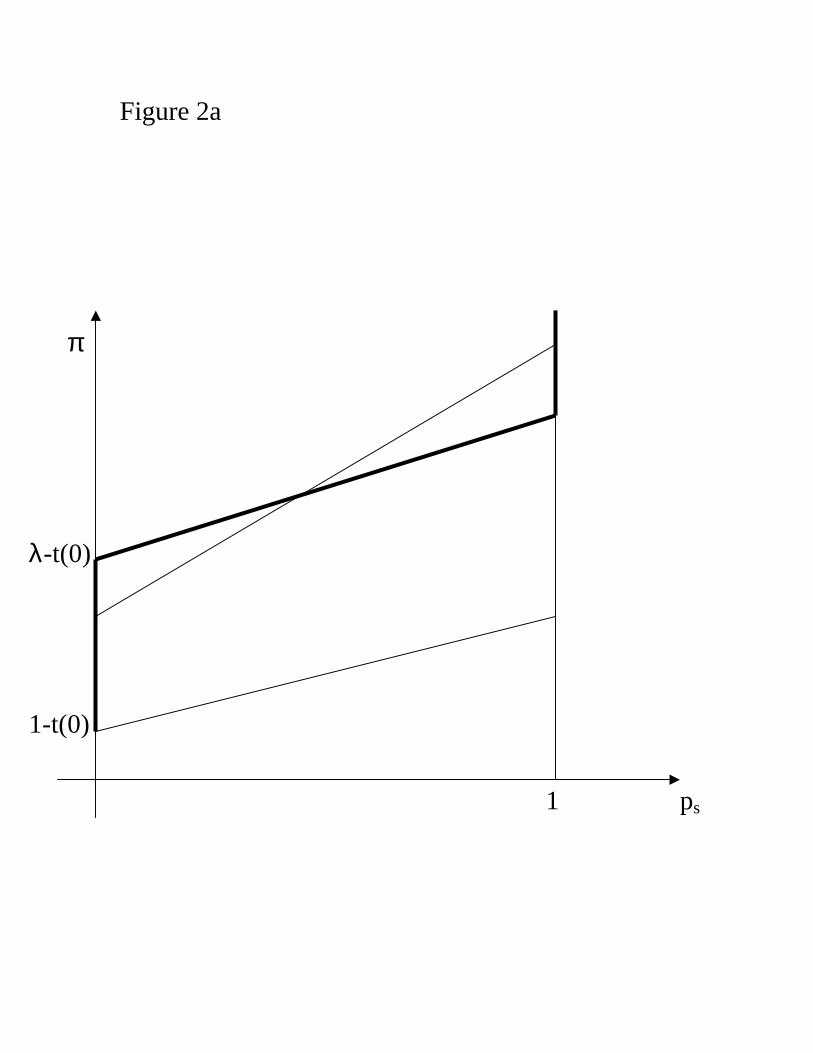
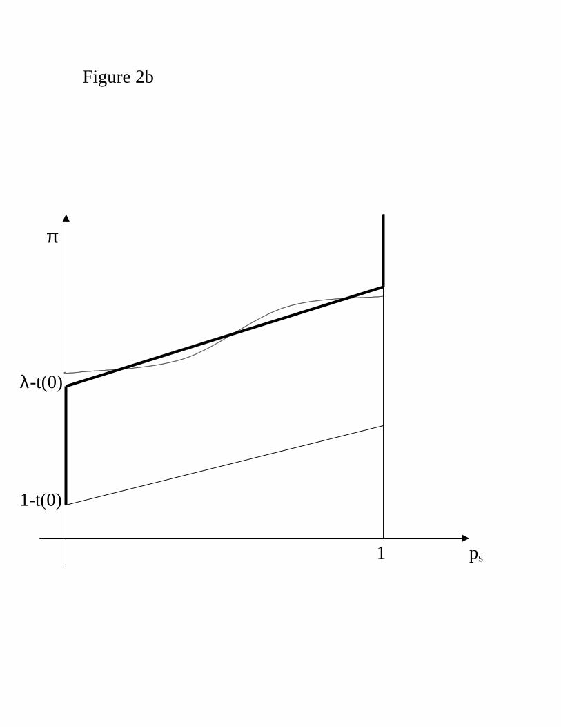
locus in Figure 1. Figure 2a provides an example in which π(ps) is linear (π(ps) = π0+π1ps).

If π0 < λ − t(0) and λ − t(1) < π0 + π1, there are three equilibria. One equilibrium is

ps = 1, another is ps = 0, and the third is given by the intersection between the π(ps) line

and the λ − t(ps) curve. This last equilibrium is unstable. Figure 2b provides an example

in which π(ps) is S-shaped, so that all three equilibria feature ps strictly between 0 and 1.

More generally, we have shown that with π endogenous there can be any (odd) number of

equilibria.17

16There are also some material rewards that might be increasing in average quality. For example, many

former office holders are invited to sit on corporate boards, become partners of law Þrms, or act as high-

proÞle lobbyists. Again, if the political class is held in disrepute it is less likely for such practices to become

widespread. On post-office Þnancial rewards see also Alesina and Spear (1988).17As we show below, our results are broadly robust to making π type-speciÞc, i.e., to a generalization in

which the rewards from office are πs(ps) for type-s citizens and πs(ps) for type-s citizens. However, in this

perfect-information world some readers might Þnd it unappealing that the rewards depend on ps at all: if

types are perfectly observed, then Þnancial and psychological rewards (though not consumption rewards)

might conceivably be completely independent of other office holders types. However, we also show below that

all our basic results go through if we introduce asymmetric information on types. In this case all that voters

know is ps, while they only have a noisy signal on each individual politicians type. Hence, the dependence of

14

3.3 Path Dependence

Another step towards a more realistic model is to endogenize the wage component of the

payoffs from holding elective office, w. We start by making explicit the cost and beneÞts of

changes in w, and relating the model with variable w to the model of the previous sections.

For simplicity, here we set π = φ so that θ = w. Increases in w beneÞt office holders, whose

payoff is w, but abstracting from the indirect effect through the quality of the elective body

potentially hurt private citizens who have to pay higher taxes.18 Denoting by τ(w) the

amount of taxes that needs to be raised to pay the p office holders a salary of w, the payoff

function for private citizens of type j becomes λj − t(ps) − τ(w). DeÞne θ(w) the functionw+ τ(w). It should be clear that everything we have said in the previous sub-sections about

the equilibrium relationship between θ and ps will apply now to the relationship between θ(w)

and ps. In particular, as θ(w) increases, the associated equilibrium value of ps is unique, and

it is identiÞed by the solid locus in Figure 1, where we now measure θ(w) on the vertical

axis. Clearly θ(w) is increasing in w, so as w varies the entire menu of potential equilibria is

feasible.19

We now turn to the task of endogenizing w. The simplest way to do so is to make the

model dynamic, and to assume that the wage of office holders at time t is decided by

majority voting by the office holders at time t−1. The population of citizens is the same inevery period, and all citizens are inÞnitely lived. In each period the citizen-candidate game

is the one analyzed above, with the difference that agents maximize a present-discounted

value of expected proÞts. The elective body decides on next periods wages at the end of its

tenure, after the public good is provided and taxes are collected. Note that with this simple

structure wt is the only state variable. This insures that within each period conditional on

π (or πs) on ps appears fully justiÞed.18We hasten to add that none of the results of this section depend on the preceived costs in terms of higher

taxes of increasing office holders salaries. While we model such costs explicitly for the sake of precision,

everything would go through if τ(w) = 0.19The government-budget constraint is taxes = f(g∗, w, ps). The discussion above implies that we are

assuming that f is separable: f(g∗, w, ps) = t(ps) + τ (w). This assumption makes the model tractable, but

we think that the intuition for the conclusions of this subsection would be robust to a more general approach.

Below we further assume that τ(0) = 0.

15

wt the equilibrium outcome is determined exactly as indicated in the previous paragraph.

In particular, higher choices for wt lead (weakly) to higher equilibrium values of ps,t. Hence,

all that is required is to analyze the wage-setting game at the end of period t.

The elective body at time t is constituted by (at most) two types of citizens, s and

s. Individuals of the same type have identical expected payoff functions. Assuming away

coordination problems all individuals of the same type will therefore vote for the same level

of wt+1. Hence, if high-ability types are in a majority in the elective body, i.e., if ps,t >12 ,

wt+1 will maximize the expected payoff of high-ability office holders. If low-ability individuals

are in the majority, or ps,t <12 , the wage maximizes expected payoffs for type-s office holders.

Furthermore, since tenure in office ends at the end of period t, the relevant payoff function

for a time-t office holder of type j coincides with the payoff function of any citizen of type j.

It will be useful to denote by w the level below which no high-ability citizen is willing to

run for office, i.e., the level at and below which Cs = ps = 0. From the previous subsections

this level is implicitly deÞned by θ(w) = λ− t(0), or

w = λ− t(0)− τ(w).

Similarly, deÞne w the level of the wage at which exactly p high-ability citizens run for office,

i.e., the case in which Cs = p and ps = 1. Again from the previous subsections w is implicitly

deÞned by the condition

w = λ− t(1)− τ(w).

Finally, deÞne w the level above which all high-ability citizens strictly prefer running for

office, or at and above which Cs = s(1 + p− v) and ps = 1.20 Clearly, w > w > w.

Starting with the case in which ps,t >12 , consider a choice of wt+1 such that w < wt+1 ≤ w.

This would imply 0 < ps,t+1 < 1. We know that in this region high-ability citizens who run

for office are assured of election and indifferent between holding public office and being

private citizens, so the expected utility of a citizen of high ability is simply wt+1. Since

20This is given by:

p

s(1+ p− v)w +µ1− p

s(1+ p− v)

¶(λ− t(1)− τ(w)− φ) = λ− t(1)− τ (w)

where the left-hand side is the expected payoff from being a candidate for office when every other high-ability

citizen is a candidate for office, and the right-hand side is the payoff of being a private citizen.

16

this is increasing in wt+1, wt+1 < w cannot be an optimal choice for next periods wage

from the point of view of a high-ability majority. Now consider a choice of wt+1 such that

w ≥ wt+1 > w, implying ps,t+1 = 1. Here high-ability citizens are indifferent between running

for (as opposed to holding) office and being private citizens, so the expected utility of a high-

ability citizen is λ − t(1) − τ(wt+1). Since this is decreasing in wt+1, wt+1 > w cannot

maximize the utility of high-ability citizens either. The perverse cases in which the preferred

choice for wt+1 for high-ability policymakers is above w or below w can be ruled out with

mild parametric restrictions.21

Now suppose that ps,t <12 , so that wt+1 maximizes the expected utility of a low-ability

citizen. Our goal is to show that low-ability citizens in the majority at time t may choose

a wt+1 different from w, the optimal choice for a high-ability majority. Hence, we limit

ourselves to providing an example in which this does indeed happen. Suppose, then, that

parameters are such that Cs = (1 − s)(1 − p − v) at w. In other words, when the wage isw, the entire low-ability population runs for office.22 The expected utility of a low-ability

citizen is then

ηw + (1− η) [1− t(0)− τ(w)− φ] ,

where η = p/[(1− s)(1 + p− v)] is the probability of election when all (and only) low-ability21The restriction to rule out choices above w is τ 0(w) > p/[s(1+ p− v)− p] for w > w and simply says that

the cost for tax payers of very high wages to politicians grows fast enough at high levels of the wage to more

than offset the gains to the select few that make it into office. To eliminate choices below w Þrst notice that

in this range high-ability citizens utility is maximized by setting w = 0. The condition for a global maximum

at w is therefore λ− t(1)− τ(w) > λ− t(0).22It follows from the previous-subsections that Cs is (weakly) increasing in w for w <w, and (weakly)

decreasing for w >w. Hence, if there are values of w such that Cs includes the entire population, w is one of

these values. In terms of the parameter space, the restriction we are imposing is that (1 − s)(1 + p − v) <p(λ− 1+ φ)/φ and use the fact that p∗s(w) = 0). If there are no such values of w, the optimal choice of wt+1

for low-ability citizens could still be different from w, potentially leading to path dependence, although for

different reasons: in that case utility at w is 1− t(0)−τ(w), which could be more than 1− t(1) − τ(w) if taxsavings on wage payments are large enough. We do not emphasize this case because it has limited empirical

relevance. It might appear disturbing that a (meaningful) path dependence result only emerges when all

low-quality citizens run for office. We have veriÞed, however, that in the more general model in which φ (or

π) takes a continuum of values with distribution G the path dependence result easily emerges irrespective of

whether all or only some of the low-quality citizens compete for office.

17

citizens run for office. None of the parametric assumptions we have imposed so far prevents

this quantity from exceeding 1 − t(1) − τ(w), which is a low-ability citizens utility whenelected officials wages are set at w. Hence, w cannot be an optimal choice of wt+1 for a

low-ability majority at time t. Furthermore, choices above w are immediately ruled out by

noting that in this region a low-ability citizens utility is 1− t(1)− τ(w). Hence, we concludethat the optimal wage for a low-ability majority, which we will denote by wl, is strictly less

than the optimal wage for a high-ability majority, w. Finally, suppose that the equilibrium

associated with wl features a low-ability majority, i.e., ps,t < 1/2 for wt = wl.23

To see how the model generates path dependence, imagine that at the time of birth of

the polity, time 0, the initial wage, w0, is selected randomly, before the Þrst citizen-candidate

game is played. It follows from the discussion above that if ps(w0) > 1/2 the Þrst assembly

will set w1 = w, with the consequence that ps,1 = 1. We would then have wt = w, ps,t = 1

for every t > 0. Instead, if p∗s(w0) < 1/2, we will have wt = wl, ps,t < 1/2 for every t. This is

our

Result 3. Path Dependence in the competence of the elected body, ps, is possible. If there is

path dependence, and ps(w0) ≤ 1/2, then ps ∈ [0, 1/2] for every t > 0. If ps(w0) > 1/2, then

ps = 1 for every t > 0.

Hence, when historical accident determines that a countrys initial political leadership

is composed by high-ability citizens, this luck tends to persist as the initial policymakers

(and all their successors) set rewards so as to insure that subsequent participants in the

political process continue to be of high quality. Instead, if initially policymakers are of low

quality, then this bad luck tends to persist, as low-quality policymakers set rewards so as to

discourage competition for office from high-quality ones. In Appendix 1 we study a special

case in detail.

23Notice that wl is not necessarily set to maximize the period t + 1 payoff function of low-ability citizens.

For, deÞne the wage that maximizes one-period-ahead payoffs w, and suppose that ps( w) > 1/2 (as it may

well be, all we know so far is that w < w, and hence ps( w) < ps(w) = 1.) Then the low-quality majority faces

a trade-off in which maximizing one-period-ahead payoffs leads to a permanent loss of majority i.e., wτ = w

for every τ ≥ t + 2. In this case, they might choose to set wl < w in order to preserve their majority. Of

course, if ps( w) ≤ 1/2 then they will set wl = w.

18

3.4 Extensions

One appealing feature of the framework developed above is that it does not invoke uncertainty

or asymmetric information to generate equilibria in which voters elect low-ability politicians.

Rather, voters have no illusions as to the intrinsic qualities of the candidates, but elect them

because they are rationed in high-quality candidates. In this subsection, however, we brießy

check that our results are robust to the addition of asymmetric information. Also, we have

assumed that market skills and policy-making competence are perfectly correlated. We brießy

discuss the case in which the correlation is imperfect. Finally, we analyze what happens when

rewards from office are type speciÞc. Our results are robust to all these extensions.

Assume that a candidates type is imperfectly observable. Citizens receive a signal about

other peoples types. SpeciÞcally, assume that if a candidate is of type i a fraction f > 0.5

of the population believes that she is of type i, and the remaining 1 − f have the wrongbelief. Consider then a situation in which Cs > 0, and Cs > 0. As before, each candidate

will vote for herself. How will non-candidates vote? Clearly each non-candidate will give her

vote to a candidate chosen randomly from the set she believes to be of high quality. Each

high-quality candidate is believed to be such by a fraction f of the non-candidates, and will

therefore receive f ∗ 100 percent of the votes. Each low-quality candidate will receive only(1−f)∗ 100 percent of the votes. Type-s candidates will therefore always receive more votesthan s types. Hence, if Cs ≥ p we have ps = 1 and Cs = 0, and if Cs < p all the high-qualitycandidates are elected for sure. This means that the analysis is identical to the one with

perfect information.

Suppose now that market productivity λi and competence when making economic-policy

decisions were only imperfectly correlated, so that there can be some individuals with low

market potential but high return in office. Under perfect information this group of people

provided it is not too small would form a perfect group of candidates: they require little

incentive to seek office, and they perform well once there. A Bad-Politicians equilibrium

would be difficult to sustain. However, if market and policy-making abilities are allowed

to differ, the assumptions on information become crucial. To see this, consider the more

realistic case in which voters observe the market productivity of a candidate (what she did

before running for office) but do not observe at the moment of voting her policy-making

19

ability. Then, as long as market and policy-making skills are positively correlated, voters

will always choose candidates with high private ability over those with low private ability.

This broadly restores the conclusions of the previous subsections, with the qualiÞcation that

ps = 1 can no longer occur, as a fraction of the elected body will always be constituted by

high-private but low-public ability citizens.

Another robustness check involves the case in which the rewards from office differ ac-

cording to the office holders type. SpeciÞcally, suppose that competent office holders receive

rewards πs, while incompetent ones receive πs, with πs and πs both potentially functions

of ps. By a line of reasoning similar to the one developed above one sees that the locus

of potential equilibria is once again limited to the solid collection of lines and segments in

Figure 1, with the vertical coordinate to be interpreted as a value of πs. Differently from

the common-π case, however, not all intersections of the πs function and the solid locus are

equilibria. SpeciÞcally, for intersections involving ps < 1, equilibrium obtains if and only if

type-s citizens weakly prefer public office to private life, i.e., if πs(ps) ≥ 1 − t(ps). If not,the positions left available for office cannot be Þlled. Note that this requirement is always

fulÞlled if πs ≥ πs, but in general it can be fulÞlled even if πs < πs. We conclude that ourbasic results survive the extension in which rewards from office are type speciÞc.

4 Corruption

A set of results analogous to the ones we have developed for the model of policy-making

competence can be derived in the context of a model of corruption. As before, we assume

that there are two types of citizens, honest, or h, and dishonest, or h. Type h is present in the

population with measure h(1 + p) and type h with measure (1− h)(1 + p). We denote by phthe fraction of office holders who are of type h. As before, we assume 1−v > h(1+p−v) > p.All citizens have the same ability. As long as a measure p of political offices are Þlled, and

the office holders provide the indispensable public good, private citizens enjoy a gross income

of λ. If the public good is not provided, private income is 0. Since competence is the same

for all policymakers, we normalize the taxes required to pay for the public good to 0.

The basic difference from the model of competence is that with corruption the payoffs

from holding public office are endogenous, and depend on a decentralized decision by each

20

individual office holder. We assume that the payoff function for a politician i of type j

is π + w + σjbi. π + w is as before the reward that is exogenous to the individual

policymaker (collected as long as g = g∗). bi measures the expected resources obtained by

harassing citizens and requiring kickbacks and bribes. σj is the exogenous parameter by which

we introduce heterogeneity in this model. Our assumption is that σh = 0, while σh = 1. In

other words, type-h citizens are high-quality because they are honest: they derive no utility

beneÞt from collecting bribes. Instead, office holders of type h are dishonest: they derive the

same utility beneÞts from resources obtained by legitimate and illegitimate means.24

A tractable way to analyze the decentralized decision of politicians is to assume that each

citizen i must interact with one office holder, and the office holder can exploit this interaction

to extract bribes. If citizen i is required to pay a bribe bi his utility is then: λ− bi. Denotethe maximum bribe a politician can collect from a citizen by b. To interpret this maximum,

one can think of a politician as facing a Laffer curve by which the returns from bribe-taking

are Þrst increasing and then decreasing. Once in office, the optimal bribe taking of a type h

politician is 0.25 As long as π does not depend on the bribe-taking activity of any individual

office holder, instead, a dishonest office holder will always maximize her revenues, thereby

setting bi = b for each citizen i he gets to victimize. Then a private citizen always prefers to

be paired with a honest politician, and since the chance of this happening is increasing in ph,

non-candidate voters will always give their preference, if given a chance, to honest candidates.

We conclude that, as in the previous section, equilibria with ph < 1 must be associated with

Ph = 1 and Ch = php, and equilibria with ph = 1 must feature Ph = Ch = 0. Note that each

politician expects to engage in 1/p interactions. Hence, bi = b/p.

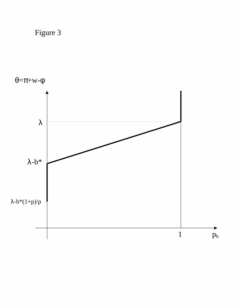
The model is summarized by Figure 3. The upward sloping line is the function phλ+(1−ph)(λ− b), which represents the (common) expected utility of private citizens as a functionof the fraction of office holders who are honest.26 On the vertical axis we measure the reward

24The qualitative results dont change if one changes the assumptions on the parameter σj , as long as

σh < σh.

25We are implicitly assuming that bribe collection involves a transaction cost ε to be borne by the politician.26It is easy to extend this model to one in which dishonest citizens prefer dishonest office-holders. As long

as the difference between a dishonest and a honest citizens utilities is small relative to the difference between

a dishonest and a honest office-holders utility, nothing changes in our results. We do not emphasize this

extension because we do not think it is very realistic. If the number of voters who would potentially prefer

21

θ = π + w − φ. The solid locus describes the equilibrium value of ph as θ varies. If θ is

above λ then honest citizens strictly prefer to be in office, so ph = 1. If λ − b ≤ θ < λ thecorresponding equilibrium value of ph obtains when honest citizens are indifferent between

private life and public office, namely when:

ph =θ + b− λ

b≡ p∗h(θ). (3)

Since all the non-candidates prefer to vote for a honest politician, all the honest citizens who

are candidates get elected, so exactly php honest citizens are candidate. When θ falls below

λ− b the equilibrium features ph = 0.27

The structure of equilibria is therefore the same as in the model of competence, with a

(weakly) monotone relationship between rewards from office θ and policymakers quality ph.

If θ is an exogenous constant the equilibrium is unique. The relevant comparative statics are

summarized by the following proposition.

Results 1’.i-1’.v. The honesty of the elected body ph is

(i) increasing in the official compensation w and in the psychological reward π,

(ii) decreasing in the cost of campaigning φ,

(iii) decreasing in the opportunity cost λ,

(iv) increasing in the cost of corruption b,

(v) decreasing in the number of seats (per capita) p.

Suppose now that the social status and legitimate private Þnancial rewards from holding

office depend on the perceived general honesty of politicians. Formally, call δh the fraction

of office holders who do not ask bribes, and assume that π = π(δh), π0(δh) > 0. Note that

whatever the value of δh, a dishonest office holder will always set b = b (thereby conÞrming

our conjecture), because her marginal impact on δh is 0. Hence, δh = ph, and we could

represent π as an upward sloping function in Figure 3. Then we have

a dishonest office-holder is large enough to matter for electoral outcomes, then it is likely that competition

among these dishonest citiznes will result in office-holders capturing all the rents from the corruption activity.

But this contradicts the assumption that dishonest citizens prefer dishonest policymakers. For discussions of

the industrial organization of corruption see Rose-Ackerman (1978) and Shleifer and Vishny (1993).

27In analogy with the previous section, we assume for simplicity that θ + b/p ≥ λ− b always.

22

Result 2’. Multiple equilibria in the honesty of the elected body ph are possible.

Equilibria correspond to intersections of the function π(·) with the function representingprivate payoffs. When the social status of politicians is low because most politicians are

corrupt, then few honest individuals are willing to participate in politics.

One might have thought that an upward sloping π function would have been sufficient to

obtain multiple equilibria in corruption even without heterogeneity in honesty. In this model

this is not true. If politicians are all potentially corrupt, they will all individually set bi = b/p,

irrespective of the amount of bribes being collected in the economy. The key insight is that

honest behavior on the part of a large number of politicians induces free riding behavior in

each individual member of the elite, and it therefore leads to underprovision of honesty. This

is not to say that one cannot write models of multiplicity of equilibria in corruption in which

there is no heterogeneity in honesty in fact, we believe it can be done 28 but simply that

a reward function that is increasing in δh is not enough.

When the model is made dynamic and wt is endogenous there is again an incentive for

dishonest policymakers to set a low wage in order to discourage honest candidates from

running for office. So let us again set π = φ, and consequently θ = w. Taking taxes into

account, the payoff function for private citizens is λ− τ(w)− (1− ph)b. Continuing to deÞneθ(w) the function w+ τ(w), the locus of possible equilibria of the within-period game is still

given by Figure 3, with θ(w) on the vertical axis. Once again, a high-quality majority will

maximize the welfare of high-quality citizens, while a low-quality majority will care about

low-quality citizens. We also re-deÞne the threshold wages w and w appropriately for the

corruption model:

w = λ− τ(w)− b.

w = λ− τ(w).

It should be clear that a high-quality majority at time t will always set wt+1 = w. The

argument is the same used in Section 3.3. But again it is possible to construct an example in

which a low-quality majority would choose a different value. In particular, if Ch = (1−h)(1+p−v) at w, the expected payoff for low-quality citizens is η(w+b/p) +(1−η)(λ−b−τ(w)−φ),

28Cadot (1987), Andvig and Moene (1990), and Tirole (1996) (who provides an instance of path dependence)

obtain multiple equilibria in models of bureaucratic corruption withn homogeneous agents.

23

which may well exceed λ− τ(w), i.e., the payoff associated with a choice of w. Hence w isnot the choice of a corrupt majority. This makes it possible for path dependence to set in,

and allows us to state

Result 3’. Path Dependence in the honesty of the elected body, ph, is possible. If there is

path dependence, and ph(w0) ≤ 1/2, then ph ∈ [0, 1/2] for every t > 0. If ph(w0) > 1/2, then

ph = 1 for every t > 0.

5 Competence and Honesty Together

This section extends the results of the previous two sections to the case in which the popu-

lation is heterogeneous in both ability and honesty. We assume that ability and honesty are

arbitrarily correlated in the population. The population continues to have measure 1 + p,

with p the measure holding office. A proportion s of the population has high ability and the

rest has low ability, in the sense of Section 3. In each ability group, a fraction h is honest and

the rest is dishonest, in the sense of Section 4. A fraction phs of the office holders has high

ability and is honest. A fraction phs is honest but of low ability. A fraction phs is dishonest

and skilled, and a fraction phs is dishonest and has low ability. We assume hs(1 + p) > p,

(1−h)s(1+p) > p, h(1−s)(1+p) > p, and (1−h)(1−s)(1+p) > p so that phs = 1, phs = 1,phs = 1 and phs = 1 are all feasible.

DeÞne ph ≡ phs + phs the fraction of politicians who are honest and ps = phs + phs thefraction with high skill. Clearly both of these quantities have a maximum at 1, and they are

both 1 only when all politicians are of type hs. The utility experienced by a private citizen

i is increasing in her ability λi, in the fraction of office holders who have high ability, and in

the fraction who are honest:

U i = λi − t(ps)− (1− ph)b. (4)

The utility experienced by an elected public officer who is honest (i.e., of type hj) is θ =

π+w−φ, which we treat as outside of her control, albeit potentially endogenous. Because πis likely to depend on (ps, ph), we will write θ(ps, ph). The utility experienced by an elected

public officer who is dishonest (of type hj) is θ + b/p > θ.

24

Now consider the space (ph, ps). The utility functions Ui can be represented in this space

by indifference curves, one set for each of the two skill types. These indifference curves are

downward sloping and, if t(ps) is convex, they are convex too (the linear and concave cases

lead to similar results). We also note that the indifference curves of skilled and honest citizens

coincide with those of skilled and dishonest; so do the indifference curves of unskilled citizens.

Notice that the indifference curves of skilled and unskilled are parallel. Honest citizens will

be indifferent between public and private life if

θ(ph, ps) = λi − t(ps)− (1− ph)b. (5)

This equation deÞnes, in the (ph, ps) space, a occupational indifference curve (henceforth

OIC), which indicates the locus of pairs (ph, ps) such that citizen i is indifferent between

private and political life. For now we impose no restrictions on these OICs. Note that, in the

special case in which θ is a constant, the OICs exactly overlay the utility indifference curves

described in the previous paragraph: i.e., for each level of θ the OIC exactly coincides with

the utility indifference curve (UIC) corresponding to a level of utility θ. OICs for dishonest

individuals can be analogously introduced as the locus satisfying:

θ(ph, ps) + b = λi − t(ps)− (1− ph)b. (6)

For pairs (ph, ps) on one side of her OIC a citizen prefers to be a office holder, while for points

on the other side she prefers to be a private citizen.

Clearly there are four OICs: for honest and competent citizens (hs), dishonest but com-

petent (hs), honest but incompetent (hs), and dishonest and incompetent (hs). A crucial

property of the two-dimensional model is that these OICs do not intersect. For by now fa-

miliar reasons, honest-skilled individuals have the most to lose and the least to gain from

political careers, so the region of the space (ph, ps) in which they prefer private life must be

the largest. Whenever (ph, ps) are such that an hs type (weakly) prefers to be in office, then

all other types strictly prefer to be in office. The relative sizes of the regions in which types

hs and hs prefer public office is in general ambiguous. Assume, to Þx ideas, that b/p > λ− 1(very little changes in the alternative scenario). Then, whenever (ph, ps) is such that hs

individuals (weakly) prefer to hold office then all hs and hs individuals strictly prefer to hold

25

public office. Finally, whenever hs types prefer office, so do hs. hs citizens prefer private life

for the smallest set of values of (ph, ps).

Some equilibrium properties are immediate. First, non-candidate voters strictly prefer

candidates of type hs to all other types. Hence, in any equilibrium featuring phs < 1 we must

have (extending the notation from the previous sections) Phs = 1 and Chs = phsp. Similarly,

if phs = 1 we must have Pij = Cij = 0, ∀ij 6= hs. Also, candidates of type hs will receive

only their own vote whenever candidates of other types are in the running.

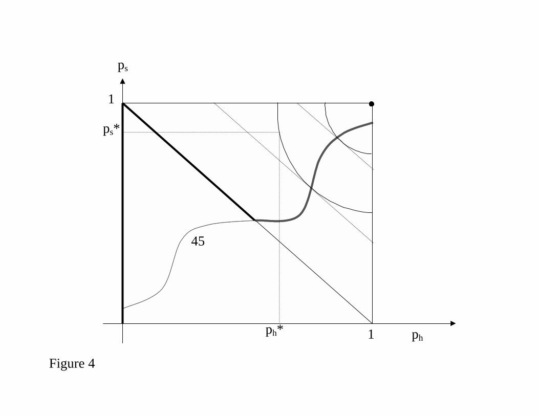
Figure 4 depicts the (ph, ps) plane. The vertical and horizontal lines through the point

(1, 1) delimit the feasible set (the point (1, 1) is reached when phs = 1). The Þgure also depicts

the line ps + ph = 1, to which we will refer to as the diagonal. The interpretation of this

line is to characterize the feasible set when phs = 0, i.e., when any increase in honesty must

be paid with a loss of competence. In other words, the line shows the best the economy

can do when its best citizens are not in politics. The Þgure also shows a map of indifference

curves, under the assumption that these have slope steeper than 45 degrees when they hit

the top side of the feasible set and slope less than 45 degrees when they hit the right side

of the set (the two alternative cases can be easily dealt with along the same lines well use

here). Then each UIC has one point at which its slope is -45 degrees. Figure 4 shows the

curve that connects all these points, called the 45 curve. The 45 curve is continuous and

upward sloping. We claim that the set of potential equilibria is restricted to the solid locus

in the Þgure, namely the point (1, 1), the part of the 45 curve to the right of the diagonal,

the part of the diagonal to the left of the 45 curve, and the vertical axis.29 We prove this

result in Appendix 2.

More speciÞcally, we prove that the model features an equilibrium for any intersection of

the hs OIC with the 45 curve above the diagonal, any intersection of the hs OIC with the

diagonal above the 45 curve, and any intersection of the hs OIC with the vertical axis. In

addition, there is an equilibrium at (1, 1) if this point lies below the hs OIC. Also (0, 0) is

an equilibrium if it lies above the hs OIC i.e., if at this point these individuals strictly

prefer private life to public office and below the OIC for citizens of type hs.

29If b/p < λ − 1 then the set of potential equilibira is given by the point (1, 1), the part of the 45 curve tothe right of the diagonal, the part of the diagonal to the right of the 45 curve, and the horizontal axis.

26

Given the above characterization the model is consistent with any number of equilibria,

from 0 to inÞnity, depending on the shape and position of the OICs of the various types. As

in the previous two models, if θ is an exogenous constant the equilibrium is always unique.

For, each of the OICs of the three types endowed with quality intersects the relevant portion

of the solid locus in Figure 4 at most once, and intersection by one precludes intersection by

the other two. Furthermore, whenever there is an equilibrium strictly within the feasible set,

the points (1, 1) and (0, 0) cannot be equilibria.

The comparative statics are completely in line with Results 1 and 1 in the upward

sloping part of the equilibrium locus. Here honesty and competence are positively correlated.

Interestingly, on the other hand, in the downward sloping segment we obtain some new

predictions. In this region a local increase in θ leads to an increase in honesty (ph), but a fall

in competence (ps). The intuition is that in such equilibria voters are constrained in honesty,

but not in competence. The convexity of the indifference curve says that voters would prefer

to move down and to the right on the diagonal. Citizens of type sh are certain of election

and indifferent between public and private life, and citizens of type sh strictly prefer private

life. An increase in θ increases the measure of hs (but not hs) candidates, allowing voters to

replace some hswith hs office holders. Similarly, in this region an increase in b will bring about

increased honesty accompanied by reduced competence. Always in this region, a paradoxical

result is that an increase in the incompetence of low-ability citizens, as measured by t(0),

leads to a decline in competence. The intuition is that increased incompetence increases type

hs citizens desire to be in office (to avoid the consequences of their own ineptitude), and this

shifts their OIC to the right, leading once again to an increase in ph accompanied by a fall in

ps. By a similar paradox, always in this downward sloping region, equilibrium competence

increases if the skilfulness of high-ability citizens at lowering taxes increases. More generally,

along this downward sloping segment honesty and competence are negatively correlated.

On the vertical segment of the equilibrium locus the elected body is formed exclusively

by citizens of types hs and hs. Here local increases in θ have the standard effect of increasing

quality (ps goes up, ph is unchanged). Changes in λ or in the parameters of t(·) have thesame effects as in Result 1. More interestingly, an increase in the cost of corruption b makes

holding office more appealing to hs and shifts their OIC upward. As a result, voters can

27

replace some hs with some hs policymaker, so that ps increases while ph does not change

(though the corruption bill increases due to the increase in b). In this region competence

and honesty are uncorrelated.

Even in the two-dimensional case multiplicity of equilibria requires that θ is endogenous,

and an increasing function of ph and ps. Recall that in this case it is no longer true that the

OICs exactly lie over some UICs. In fact, there is no restriction whatsoever on the shape of

the OICs: they could be decreasing, increasing, non-monotonic, and even backward bending.

In this case, if the OIC for the hs has upward sloping portions, it might well intersect the

segment of the 45 curve above the diagonal more than once. If the OIC for the hs has

downward sloping portions, it might well intersect the segment of the diagonal above the 45

curve more than once. The OIC for the hsmight well hit the vertical axis more than once also.

The key conclusion is, therefore, that it is perfectly possible for otherwise identical countries

to be on different equilibria and to Þnd no cross-country correlation between honesty and

ability.30

6 Conclusions

We have investigated the mechanisms that lead to the selection of citizens of varying quality

into political life. Countries may Þnd themselves stuck in bad equilibria such that high-quality

citizens avoid public office because so do other high-quality citizens. Also, countries may

experience persistent low quality of the policymaking class, whereby low-quality policymakers

in one period set up next periods incentives so as to keep high-quality ones from seeking

office. As a result, otherwise identical countries can experience different average levels of

competence and/or honesty of the political class.

30We have not formally investigated the case of endogenous w, but it seems to us that once again

policymakers with relatively lower quality have an incentive to discourage participation by candidates of

relatively higher quality. Hence, path dependence should again be a possibility. Additional sources of path

dependence may arise if, as seems realistic, corruption costs are higher for rich (high-ability) citizens than

for poor (low-ability) ones. In particular, low-skill citizens will be extremely averse to paying high salaries to

office holders (since they are not affected by corruption) whereas high-skill citizens will be willing to pay high

salaries to stem corruption. Low- (high-) ability majorities would then choose low (high) wages.

28

References

Ades, A. and R. Di Tella (1997): The New Economics of Corruption: a Survey and some

New Results, Political Studies, XLV, 496-515.

Alesina, A. and H. Rosenthal (1995): Partisan Politics, Divided Government, and the

Economy, Cambridge University Press.

Alesina, A. and H. Rosenthal (1996): A Theory of Divided Government, Econometrica,

64, 1311-41.

Alesina, A., N. Roubini, and G. Cohen (1997): Political Cycles and the Macroeconomy,

MIT Press.

Alesina, A., and S. Spear (1988): An Overlapping Generations Model of Electoral Com-

petition, Journal of Public Economics, 37, 359-379.

Andvig, J.C., and K. Moene (1990): How Corruption May Corrupt, Journal of Eco-

nomic Behavior & Organization, 13, 63-76.

Bardhan, P. (1997): Corruption and Development: A Review of Issues, Journal of

Economic Literature, XXXV, 1320-1346.

Becker, G. and C. Mulligan (1998): Deadweight Costs and the Size of Government,

NBER Working Paper No. 6789.

Besley, T.J.. and S. Coate (1997): An Economic Model of Representative Democracy,

Quarterly Journal of Economics, CXII, 85-114.

Besley, T.J.. and S. Coate (1998): Sources of Inefficiency in a Representative Democracy:

A Dynamic Analysis, American Economic Review, 88, 139-156.

Besley, T.J. and J. McLaren (1993): Taxes and Bribery: The Role of Wage Incentives,

Economic Journal, 103, 119-141.

Cadot, O. (1987): Corruption as a Gamble, Journal of Public Economics, 32, 223-44.

Charap, J. and C. Harm (1999): Institutionalized Corruption and the Kleptocratic

State, IMF Working Paper.

Cukierman, A. and A. Meltzer (1986): A Positive Theory of Discretionary Policy, the

Cost of Democratic Government, and the BeneÞts of a Constitution, Economic Inquiry, 24,

367-388.

Dal Bo, E. and R. Di Tella (1999): Democracy under Pressure: Political Parties vs.

29

Nasty Interest Groups, unpublished, Harvard University.

Hines, J. (1995): Forbidden Payment: Foreign Bribery and American Business Since

1977, NBER Working Paper No. 5266.

Kaufmann, D. (1997): Some Myths and Facts, Foreign Policy, Summer, 114-131.

Kaufmann, D. and S. Wei (1999): Does Grease Money Speed Up the Wheels of

Commerce? NBER Working Paper No. 7093.

La Porta, R., F. Lopez-De-Silanes, A. Shleifer, and R. Vishny (1998): The Quality of

Government, NBER Working Paper 6727.

Mauro, P. (1995): Corruption and Growth, Quarterly Journal of Economics, CXI,

681-712.

Myerson, R.B. (1993): Effectiveness of Electoral Systems for Reducing Government

Corruption, a Game-Theoretic Analysis, Games and Economic Behavior 5, 118-132.

Myrdal, G. (1968): Asian Drama: An Inquiry into the Poverty of Nations, Pantheon

Books.

Osborne, M.J. and A. Slivinski (1996): A Model of Political Competition with Citizen

Candidates, Quarterly Journal of Economics, CXI, 65-96.

Persson, T. and G. Tabellini (1990), Macroeconomic Policy, Credibility, and Politics,

Harwood Academic Publishers.

Rogoff, K. and A. Sibert (1988), Elections and Macroeconomic Policy Cycles, Review

of Economic Studies, 55, 1-16.

Rogoff, K. (1990), Equilibrium Political Budget Cycles, American Economic Review,

80, 21-36.

Rose-Ackerman, S. (1978): Corruption: A Study in Political Economy, Academic Press.

Shleifer, A. and R. Vishny (1993): Corruption, Quarterly Journal of Economics, 108,

599-617.

Tanzi, V. (1997), Corruption around the World, IMF Staff Papers, 45, 559-594.

Tirole, J. (1996): A Theory of Collective Reputations, Review of Economic Studies, 63,

1-22.

Wei, S. (1997), How Taxing is Corruption on International Investors? NBER Working

Paper No. 6030.

30

Appendix 1: Path Dependence in the Linear Case

This section studies in greater detail the example of path dependence of Section 3.3 for

the special case in which

t(ps) = β − γps (7)

and

τ(w) = δw. (8)

In this case we have (recall that we have normalized π = φ)

w = λ− (β − γ)− δw = λ− β + γ1 + δ

and

w = λ− β − δw = λ− β1 + δ

low-ability citizens expected utility when w = w is

Us(w) = 1− β + γ − δλ− β + γ1 + δ

=1+ δ(1− λ)− β + γ

1 + δ.

As discussed in Section 3.3, under the assumption that η(λ − 1 + φ)/φ > 1 all low-ability

citizens run for office at w. Hence, their expected utility is

Us(w) = ηλ− β1 + δ

+ (1− η)µ1− β − δλ− β

1 + δ− φ

¶=

1 + δ(1− λ)− β + η(1 + δ)(λ− 1 + φ)− (1 + δ)φ1 + δ

.

Now suppose that Us(w) < Us(w), or

η(1 + δ)(λ− 1 + φ)− (1 + δ)φ > γ (9)

which is certainly possible. Notice that the condition is more likely to be satisÞed if η is

large (a large probability of election when competing with only low-skill candidates makes

the competition more worthwhile), if λ is large (a large λ implies a large w, so being in office

is more valuable we are assuming that δ is small, which is likely), and if φ is small (obvious).

It is less likely to be satisÞed if γ is large (as in this case it is very valuable to have good

politicians in office in case of defeat at the election).

31

Suppose then that the above condition is satisÞed, and suppose that the wage is set to

maximize the per-period utility of low-ability citizens. We can show that if δ is sufficiently

small the wage will then be (permanently) set at w. To the left of w low-skill citizens

utility is ηw + (1 − η)(1 − β − δw), which is increasing in w for δ small. To the right of wtheir utility is 1− β + γ − δw, which is decreasing in w. Hence, the optimal choice is in theinterval [w,w). On this interval, expected utility as long as all are running is

Us(w) = η(1− ps)w+ [1− η(1− ps)] [1− β + γps − δw − φ].

Now notice that on this interval we have w = λ− t(ps)− τ(w), which becomes (using (7) and(8))

ps =1

γ[(1 + δ)w + β − λ].

Substituting and simplifying we then have

Us(w) = w−½1− η + η 1

γ[(1 + δ)w + β − λ]

¾(λ− 1 + φ)

which is linear in w. The slope of this function is:

1− η 1γ(1 + δ)(λ− 1 + φ)

which has the same sign as

γ − η(1 + δ)(λ− 1 + φ)

which is negative because of restriction (9).

Intuitively, restriction (9) says that low-ability citizens prefer the equilibrium associated

with w to the one associated with w. In turn, the latter must be strictly better than the

situation in which the wage is w and all low-quality citizens run for office. But since utility

conditional on everybody running is linear, if the slope was positive we would have a

contradiction.

Since the slope of the objective function is negative on [w,w) the optimal choice is w.

Since here ps = 0, we have path dependence.

32

Appendix 2: Analysis of two-dimensional case.

Let us Þrst discuss candidate equilibria above the diagonal, such as, for example, point

(p∗h, p∗s) in Figure 4. First, for this to be an equilibrium it must necessarily feature phs > 0, as

points in this region are unattainable without hs types in office. Then, the OIC for hs types

would pass for this point, as an equilibrium (other than (1, 1)) in this region requires these

types to be certain of election and therefore indifferent between public and private jobs. But

if the hs types are indifferent between private and public jobs then all other types strictly

prefer being office holders. Given this strict preference, the point under consideration can

be an equilibrium only if such types are uncertain of election. In particular, the measure

of candidates of these two types will be determined by a condition stating that given the

probability of being elected (itself a function of the measure of candidates) and the cost of

running φ such individuals strictly prefer or are indifferent between running for office or not.

In other words, there is excess supply of hs and hs types. In turn, this implies that there

cannot be citizens of type hs holding office. Given our assumption of conditionally sincere

voting, non-candidates will always vote in a way that all positions are Þlled by candidates

with at least one quality. For example, there cannot be an equilibrium in which all non-

candidates vote for types hs, and all other types have therefore equal probability of being

elected. For, in this case, some of the non-candidates have a dominating voting deviation in

which instead of voting for an hs type they vote for a hs or a hs type.

In summary, any candidate equilibrium above the diagonal features phs = Phs = Chs = 0.

Then, point (p∗h, p∗s) is supported by a unique combination of shares of citizens of the various

types holding office. For a point (p∗h, p∗s) this combination is the solution to the system of

three equations in three unknowns phs + phs = p∗h, phs + phs = p

∗s, and phs + phs + phs = 1.

We can now argue that if (p∗h, p∗s) is outside of the 45 curve it cannot be part of an

equilibrium. Recall that outside of the 45 curve the UICs have slope different from -45

degrees. Suppose it is steeper. Then there must necessarily be at least one non-candidate

who could deviate from his voting strategy and transfer his vote from a winning candidate

of type hs to a losing candidate of type hs. Should this deviation prove pivotal, this voter

would have moved the equilibrium down and to the right along a -45 degree line. But

such a move would determine an increase in utility for the voter, as it would take him to

33

a higher indifference curve. Hence, this voting deviation is proÞtable (in the conditionally

sincere sense) and the equilibrium is broken. Of course, if at a point above the diagonal the

indifference curve is ßatter than -45 degrees, the equilibrium breaking deviation is to vote for

a candidate of type hs over a candidate of type hs.

Now let us focus on candidate equilibria below the diagonal. For such a point to be an

equilibrium, at least one of the three types having at least one quality must strictly prefer to

hold office. If none did, then types hs and hs would for sure strictly prefer private life. But

then no point with ph > 0 would be feasible. This strict preference for office implies that

at least one of the three desirable types is in excess supply, in the sense that some of the

candidates of this type do not get elected. But at the same time we have ph + ps < 1, as we

are below the diagonal, so there must be some hs types in office. This is inconsistent with

our equilibrium concept as voters would then deviate in such a way to replace some of the

hs office holders with candidates of more desirable type.

Next, we consider points on the diagonal to the right of the 45 line. If a point in this

region were an equilibrium, and it featured hs types in office, then it would also have to

feature some hs in office, otherwise the shares of the four types holding office could not add

up to 1. But if some hs citizen is in office then types hs and hs must strictly prefer to hold

office, so voters once again have a dominating conditionally sincere deviation. Hence, this

equilibrium could never feature phs > 0, and since we must have ph + ps = 1 this means

there can be no hs types in office. Next note that for this to be an equilibrium, citizens

of type hs must weakly prefer being office holders (otherwise ph = 0), which implies that

citizens of type hs strictly prefer to hold public office (recall our assumption on the ranking of

OICs). Hence, candidates of type hs are in excess supply, and voters have access to a voting

deviation moving up and to the left on the diagonal. By deÞnition of the 45 curve such a

deviation dominates in as if pivotal sense the point under consideration, and this cannot

be an equilibrium. A very similar argument can be used to rule out points on the horizontal

axis, where we have ps = 0, the hs types have a strict preference for holding office, and the

UIC has slope less than 45 degrees.

Up to now we have eliminated all points not on the solid locus in Figure 4. We now

discuss the conditions under which points on the solid locus are equilibria. Points on the 45

34

curve above the diagonal are equilibria if and only if they also lie on the OIC of hs types. If

they do not (only if) then either the hs types strictly prefer office (in which case we would

jump to (1, 1)), or they strictly prefer private life (in which case the point is unfeasible). If

they do (if) citizens of type hs are indifferent between holding office and living private lives,

and those who are candidates are all elected and have no incentive to deviate. The other two

one-quality types strictly prefer office and are in excess supply: their participation to the

elections determined by the condition that given the probability of election and the cost of

running they weakly prefer to be candidates. Citizens of type hs are non-candidates. And

non-candidates have no dominating conditionally sincere voting deviation as the indifference

curve lies entirely above the 45 degree line through this point.

Consider now the diagonal above the 45 curve. The claim is that points in this region are

equilibria if and only if they also lie on the OIC of type hs citizens. By the same argument

used for the section of the diagonal below the 45 curve, equilibria on this locus must feature

phs = phs = 0. Then we must have that citizens hs weakly prefer being in office (otherwise

ph = 0), which implies that citizens hs have a strict preference for public service. Now if

the hss preference were strict, so that candidates of this type were in excess supply, then a

voting deviation down and to the right on the diagonal would be feasible. But by deÞnition

of the 45 curve such a deviation weakly dominates the point under consideration. This shows

that hs citizens must be indifferent between private and public life, i.e., the only if part of

our claim. Now if the hs are exactly indifferent between private and public life the number of

candidates is equal to the number of elected individuals of this type, and a voting deviation

down and to the right (the only one attractive) is unfeasible. This proves the if part of the

claim.

We are left with the vertical axis. Points on the vertical axis are equilibria if and only if

they also lie on the OIC of citizens of type hs. If they are above it they are unfeasible, as no

person of high ability would agree to stay in office. If they are below it, then hs candidates

would be in excess supply, and it would be possible to replace some of the hs office holders

(who necessarily hold office in this region). On points on the hss OIC, instead, the number

of hs candidates is equal to the number of hs winners. The other types with at least one

quality strictly prefer private life (and are not candidate) and the types with no quality are

35

rationed on political jobs. No dominating conditionally sincere voting deviation exists.

36

Figure 1

ps

θ=π+w-φ

1

λ-t(0)

1-t(0)

Figure 2a

ps

π

1

λ-t(0)

1-t(0)

Figure 2b

ps

π

1

λ-t(0)

1-t(0)

Figure 3

ph

θ=π+w-φ

1

λ-b*

λ

λ-b*(1+p)/p

Figure 4

1

1

ps

ph

45

ph*

ps*