1 Worms at Work: Long-run Impacts of Child Health Gains * Sarah Baird Joan Hamory Hicks George Washington University University of California, Berkeley CEGA Michael Kremer Edward Miguel Harvard University and NBER University of California, Berkeley and NBER First version: October 2010 This version: March 2011 Abstract: The question of whether – and how much – child health gains improve adult living standards is of major intellectual interest and public policy importance. We exploit a prospective study of deworming in Kenya that began in 1998, and utilize a new dataset with an effective tracking rate of 83% over a decade, at which point most subjects were 19 to 26 years old. Treatment individuals received two to three more years of deworming than the comparison group. Among those with wage employment, earnings are 21 to 29% higher in the treatment group, hours worked increase by 12%, and work days lost to illness fall by a third. A large share of the earnings gains are explained by sectoral shifts, for instance, through a doubling of manufacturing employment and a drop in casual labor. Small business performance also improves significantly among the self-employed. Total years enrolled in school, test scores and self-reported health improve significantly, suggesting that both education and health gains are plausible channels. Deworming has very high social returns, with conservative benefit-cost ratio estimates ranging from 24.7 to 41.6. * Acknowledgements: Chris Blattman, Hana Brown, Lorenzo Casaburi, Lisa Chen, Garret Christensen, Lauren Falcao, Francois Gerard, Eva Arceo Gomez, Jonas Hjort, Maryam Janani, Andrew Fischer Lees, Jamie McCasland, Owen Ozier, Changcheng Song, Sebastian Stumpner, Paul Wang, and Ethan Yeh provided excellent research assistance on the KLPS project. We thank Michael Anderson, Jere Behrman, Alain de Janvry, Erica Field, Fred Finan, Michael Greenstone, Isaac Mbiti, T. Paul Schultz, and John Strauss, and seminar participants at U.C. Berkeley, USC, Harvard, the J-PAL Africa Conference, the Pacific Conference on Development Economics, and UCSF for helpful suggestions. We gratefully acknowledge our NGO collaborators (International Child Support and Innovations for Poverty Action Kenya), and funding from NIH grants R01-TW05612 and R01-HD044475, NSF grants SES-0418110 and SES-0962614, the World Bank, the Social Science Research Council, and the Berkeley Population Center. All errors remain our own.
Worms at Work: Long-run Impacts of Child Health Gains*
Sarah Baird Joan Hamory HicksGeorge Washington University University of California, Berkeley CEGA
Michael Kremer Edward MiguelHarvard University and NBER University of California, Berkeley and NBER
First version: October 2010This version: March 2011
Abstract: The question of whether – and how much – child health gains improve adult livingstandards is of major intellectual interest and public policy importance. We exploit aprospective study of deworming in Kenya that began in 1998, and utilize a new dataset withan effective tracking rate of 83% over a decade, at which point most subjects were 19 to 26years old. Treatment individuals received two to three more years of deworming than thecomparison group. Among those with wage employment, earnings are 21 to 29% higher inthe treatment group, hours worked increase by 12%, and work days lost to illness fall by a
third. A large share of the earnings gains are explained by sectoral shifts, for instance,through a doubling of manufacturing employment and a drop in casual labor. Small businessperformance also improves significantly among the self-employed. Total years enrolled inschool, test scores and self-reported health improve significantly, suggesting that botheducation and health gains are plausible channels. Deworming has very high social returns,with conservative benefit-cost ratio estimates ranging from 24.7 to 41.6.
* Acknowledgements: Chris Blattman, Hana Brown, Lorenzo Casaburi, Lisa Chen, Garret Christensen, LaurenFalcao, Francois Gerard, Eva Arceo Gomez, Jonas Hjort, Maryam Janani, Andrew Fischer Lees, Jamie McCasland,Owen Ozier, Changcheng Song, Sebastian Stumpner, Paul Wang, and Ethan Yeh provided excellent researchassistance on the KLPS project. We thank Michael Anderson, Jere Behrman, Alain de Janvry, Erica Field, FredFinan, Michael Greenstone, Isaac Mbiti, T. Paul Schultz, and John Strauss, and seminar participants at U.C.Berkeley, USC, Harvard, the J-PAL Africa Conference, the Pacific Conference on Development Economics, andUCSF for helpful suggestions. We gratefully acknowledge our NGO collaborators (International Child Support andInnovations for Poverty Action Kenya), and funding from NIH grants R01-TW05612 and R01-HD044475, NSFgrants SES-0418110 and SES-0962614, the World Bank, the Social Science Research Council, and the BerkeleyPopulation Center. All errors remain our own.
The question of whether – and how much – child health gains improve adult living standards is of
major intellectual interest and public policy importance. The belief that childhood health investments
have large payoffs in terms of adult living standards underlies government and foreign aid donor
school health and nutrition programs in many less developed countries. In the absence of such public
subsidies, standard models imply that productive child health investments might go unexploited in
settings where infectious diseases are widespread, if treatment generates broader social benefits that
households do not internalize. Yet the well-known methodological challenges to studying this issue –
including the scarcity of both experimental variation in health investments and panel datasets
tracking children into adulthood, and research designs that do not allow for the estimation of
epidemiological externalities – have limited research progress.
We exploit a prospective experiment that provided deworming treatment to children in rural
Kenyan schools starting in 1998, and utilize a new longitudinal dataset with an effective tracking rate
of 83% among a representative subset of individuals enrolled in these schools over a decade (to
2007-09), at which point most subjects were young adults between 19 to 26 years of age. The
combination of prospective variation in child health investments with a long-term panel dataset
featuring high tracking rates, together with our ability to estimate spillover benefits of deworming
treatment, sets this study apart from most of the existing literature.
Intestinal worm infections – including hookworm, whipworm, roundworm and schistosomiasis
– are among the world’s most widespread diseases, with roughly one in four people infected (Bundy1994, de Silva et al. 2003). School age children have the highest infection prevalence of any group,
and baseline infection rates in our Kenya study area are over 90%. Although light worm infections
are often asymptomatic, more intense infections can lead to lethargy, anemia and growth stunting.
Fortunately, worm infections can be treated infrequently (once to twice per year) with cheap and safe
drugs. There is a growing body of evidence that school-based deworming in African settings can
generate immediate improvements in child appetite, growth and physical fitness (Stephenson et al.
1993), and large reductions in anemia (Guyatt et al. 2001, Stoltzfus et al. 1997). Treating worm
infections also appears to strengthen children’s immunological response to other infections,
potentially producing much broader health benefits in regions with a high tropical disease burden.
For instance, a recent double-blind placebo controlled randomized trial among Nigerian preschool
children finds that children who received deworming treatment for 14 months show reduced infection
prevalence with Plasmodium, the malaria parasite (Kirwan et al. 2010), and other authors have
hypothesized that deworming might even provide some protection against HIV infection (e.g., see
Fincham et al. 2003, Hotez and Ferris 2006, Watson and John-Stewart 2007).
Due to the experimental design, deworming treatment group individuals in our sample received
two to three more years of deworming than the control group. Previous work in this sample shows
that deworming treatment led to large medium-run gains in school attendance and health outcomes,
and, due to worms’ infectious nature, that sizeable externality benefits accrued to the untreated
within treatment communities and to those living near treatment schools (Miguel and Kremer 2004),
as well as to the younger siblings of the treated (Ozier 2010).
In this paper, we generate unbiased estimates of the average impact of deworming on long-run
outcomes by comparing the program treatment and control groups during 2007 to 2009. Among
those with wage employment, we find that earnings are 21 to 29% higher in the deworming treatment
group, while hours worked increase by 12% and work days lost to illness fall by a third. There is
suggestive evidence that deworming also generated positive externalities on labor market outcomes,
although these spillover effects are relatively imprecisely estimated.
These labor market gains are accompanied by marked shifts in employment sector for the
treatment group, with more than a doubling of well-paid manufacturing jobs (especially among
males) and declines in both casual labor and domestic services employment. Changes in the
subsector of employment account for nearly all of the earnings gains in deworming treatment group
in a Oaxaca-style decomposition. This pattern indicates that health investments not only boost
productivity and work capacity in existing activities, but, by leading individuals to shift into morelucrative economic activities (like manufacturing employment), may also contribute to the structural
transformation of the economy a whole. Understanding how to promote this transition has long been
a central theme within development economics (see Lewis 1954, among many others), and our
results provide a piece of suggestive evidence that health investments may speed this transition.
Measuring labor productivity is more challenging for the majority of our subjects who were
either self-employed or working in subsistence agriculture, rather than working for wages, although
even in these groups there is evidence of positive impacts. The estimated impacts on the small
business performance of the self-employed, namely measures of profits and employees hired, are also
positive and relatively large in magnitude. Total hours worked in any occupation was significantly
higher in the treatment group, with particularly large gains in hours worked among the self-
employed. The number of meals the respondent ate yesterday is also significantly higher in the
treatment group, consistent with higher living standards.
We present a simple model (building on Bleakley 2010) to illustrate the conditions under which
health and education gains might drive higher earnings. We find empirically that the total years
enrolled in school increased, by approximately 0.3 years, some test scores rose, and self-reported
health improved in the treatment group. Although we cannot convincingly decompose how much of
our earnings gains are working through education versus health without imposing considerably
stronger assumptions, these findings suggest that both channels are likely playing some role.
Deworming appears to have very high social returns. Considering only the earnings gains
among the subset of wage earners, and taking into account the costs of drug treatment, the
opportunity cost of additional time spent in school rather than working, and implicit congestion costs
on the educational system from higher school attendance, conservative estimates of the benefit-cost
ratio for deworming investments range from 24.7 to 41.6, depending on whether only wage
productivity gains (per hour worked) are considered or if total earnings are assumed to capture
benefits, respectively. The latter approach may be appropriate if better health improves the capacity
to work longer hours, as in the original formulation of health capital in Grossman (1972), who argues
that it is precisely this increase in “non-sick” time that distinguishes health investments from other
types of human capital investment.
Our findings contribute to several strands of existing work. The most closely related studies are
by Bleakley (2007a, 2007b, 2010), who examines the impact of a large-scale deworming campaign in
the U.S. South during the early 20th century on schooling and adult earnings, by comparing heavily
infected versus lightly infected regions over time in a difference-in-difference design. He finds thatdeworming raised adult income by roughly 17%, and, extrapolating these findings to the even higher
worm infection rates found in tropical Africa, estimates that deworming in Africa could lead to
income gains of 24%. Remarkably, given the gap in time and space between his setting and ours, this
falls squarely in the range (21 to 29%) of our estimated earnings gains. Early work by Schapiro
(1919) using a simpler first-difference research design found wage gains of 15-27% on Costa Rican
plantations after workers received deworming treatment. Taken together, these findings lend
credence to the view that treating intestinal worm infections can substantially increase labor
productivity.1 As Bleakley (2010) notes, the fact that deworming reduces morbidity but has
negligible effects on mortality means it is particularly likely to boost per capita living standards.
1 There remains a lively debate in the public health and nutrition literatures about the cost-effectiveness of deworming treatment (as surveyed in Taylor-Robinson et al. 2007). In earlier work in economics, Weisbrod et al(1973) document relatively weak cross-sectional correlations between worm infections and labor productivity, testscores, fertility, and mortality in St. Lucia. Bundy et al. (2009) argue that many existing studies understate thedeworming’s benefits since they fail to consider treatment externalities (and so understate true treatment effects) by
Beyond deworming, our findings contribute to the growing literature on the long-run economic
impacts of early life health and nutrition shocks. The well-known INCAP experiment in Guatemala
described in Hodinott et al. (2008), Maluccio et al. (2009), and Behrman et al. (2009) provided
nutritional supplementation to two villages while two others served as a control, and finds gains in
male wages of one third, improved cognitive skills among both men and women, and positive
intergenerational effects on the nutrition of beneficiaries’ children. Beyond the small sample size of
four villages, a limitation of the INCAP studies is their relatively high attrition rate over the
approximately 35 years of follow-up surveys, at roughly 40%. A series of other influential studies
have shown large long-run economic impacts of in utero or child health and nutrition shocks
resulting from natural experiments, including the worldwide influenza epidemic of 1918 (Almond
2006), war-induced famine in Zimbabwe (Alderman et al., 2006a), and economic shocks driven by
rainfall variation in Indonesia (Maccini and Yang, 2009).2 While many studies argue that early
childhood health gains in utero or before age three have the largest impacts (World Bank 2006 and
Hodinott et al. 2008 are but two examples), our findings show that even health investments made in
school aged children can have important effects.3
The rest of the paper is organized as follows. Section 2 presents background on the school
deworming project and the follow-up survey. Section 3 lays out the estimation strategy and describes
the impacts of deworming on labor market outcomes, while Section 4 focuses on effects on education
and health. Section 5 computes the social returns to deworming investment, and the final section
concludes, discussing external validity and implications for ongoing research and for public policy.
using designs that randomize within schools; focus almost exclusively on biomedical criteria and ignore cognitive,education and income gains that are a key component of overall benefits; and do not deal adequately with high ratesof attrition. The current paper attempts to address these three concerns. Beyond Miguel and Kremer (2004) and thecurrent paper, Alderman et al. (2006b) and Alderman (2007) also use a cluster randomized controlled design andfind large positive child weight gains in Uganda.2 Other studies in less developed countries that attempt to address the issue of long-run impacts of child health arethose that deal with low birthweight (Sorenson et al., 1997; Conley and Bennett, 2000); iodine deficiency in utero (Xue-Yi et al., 1994; Pharoah and Connolly, 1991; Field et al., 2007) and in early childhood (Fernald andGrantham-McGregor, 1998); whether children were breastfed (Reynolds, 2001); early childhoold malariaprophylazis, and early childhood under nutrition (Alderman et al., 2003; Mendez and Adair, 1999; Glewee et al., 2001), among many others. Though these studies are generally non-experimental (Jukes et al., 2006 is an
exception), taken together they provide considerable evidence that adult cognitive performance may be affected bynutrition in the womb and early childhood. Related work on the long-run benefits of child health and nutritioninvestments in the U.S. include Currie and Thomas (1995), Currie, Garces and Thomas (2002), and Case and Paxson(2010). Other noteworthy micro-empirical contributions on nutrition, health and productivity include Schultz (2005),Alderman (2007), Thomas et al. (2008), and Pitt, Rosenzweig and Hassan (2011), and recent contributions inmacroeconomics on health and economic growth include Acemoglu and Johnson (2007), Ashraf, Lester and Weil(2009), and Aghion, Howitt and Murtin (2010).3 As discussed below, we do not find evidence of heterogeneous treatment effects by age or gender, but there issuggestive evidence that gains in work hours are larger among those who were younger when they receiveddeworming, perhaps because the resulting health gains are somewhat larger earlier in life.
2. Background on the Primary School Deworming Program and Kenya Life Panel Survey
This section describes the study site, the deworming experiment, and follow-up survey, including our
respondent tracking approach. We then present sample summary statistics.
2.1 The Primary School Deworming Program (PSDP)
In 1998, the non-governmental organization ICS launched the Primary School Deworming Program
(PSDP) to provide deworming medication to individuals enrolled in 75 primary schools in Busia
District, a densely-settled farming region of rural western Kenya adjacent to Lake Victoria. The
schools participating in the program consisted of 75 of the 89 primary schools in Budalangi and
Funyula divisions in southern Busia (with 14 town schools, all-girls schools, geographically remote
schools, and program pilot schools excluded), and contained 32,565 pupils at baseline.
Parasitological surveys conducted by the Kenyan Ministry of Health indicated that these divisions
had high baseline helminth infection rates at over 90%. Using modified WHO infection thresholds
(described in Brooker et al. 2000a), over one third of children in the sample had “moderate to heavy”
infections with at least one helminth at the time of the baseline survey, a high rate but one not
atypical in African settings (Brooker et al. 2000b). The 1998 Kenya Demographic and Health Survey
indicates that 85% of 8 to 18 year old children in western Kenya were enrolled in school, indicating
that our school-based sample is broadly representative of western Kenyan children as a whole.
Busia is close to the Kenyan national mean along a variety of economic and social measures.The 2005 Kenya Integrated Household Budget Survey shows that 96% of children aged 6 to 17 in
Busia had “ever attended” school compared to 93% nationally, the gross enrollment rate was 119
compared to 117 nationally, while 75% of Busia adults were literate versus 80% nationally.
However, Busia is poorer than average: 62% of Busia households fall below the poverty line
compared to 41% nationally. Given that Kenyan per capita income is somewhat above the sub-
Saharan African average (if South Africa is excluded), the fact that Busia is slightly poorer than the
Kenyan average probably makes the district more representative of rural Africa as a whole.
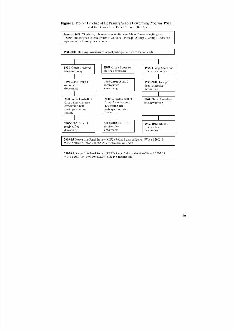
The 75 schools involved in this program were experimentally divided into three groups
(Groups 1, 2, and 3) of 25 schools each: the schools were first stratified by administrative sub-unit
(zone), listed alphabetically by zone, and were then listed in order of enrollment within each zone,
and every third school was assigned to a given program group; supplementary appendix A contains a
detailed description of the experimental design. The groups are well-balanced along baseline
demographic and educational characteristics, both in terms of mean differences and distributions,
where we assess the latter with the Kolmogorov-Smirnov test of the equality of distributions (Table
1).4 The same balance is also evident among the subsample of respondents currently working for
wages (see Supplementary Appendix Table A1).
Due to the NGO’s administrative and financial constraints, the schools were phased into the
deworming program over the course of 1998-2001 one group at a time. This prospective and
staggered phase-in is central to this paper’s econometric identification strategy. Group 1 schools
began receiving free deworming treatment in 1998, Group 2 schools in 1999, while Group 3 schools
began receiving treatment in 2001; see Figure 1. The project design implies that in 1998, Group 1
schools were treatment schools while Group 2 and 3 schools were the comparison schools, and in
1999 and 2000, Group 1 and 2 schools were the treatment schools and Group 3 schools were
comparison schools, and so on. The NGO typically requires cost sharing, and in 2001, a randomly
chosen half of the Group 1 and Group 2 schools took part in a cost-sharing program in which parents
had to pay a small positive price to purchase the drugs, while the other half of Group 1 and 2 schools
received free treatment (as did all Group 3 schools). Kremer and Miguel (2007) show that cost-
sharing led to a sharp reduction in deworming treatment rates by 60 percentage points, introducing
further exogenous variation in deworming treatment that we can exploit. In 2002 and 2003, all
sample schools received free treatment.
Children in Group 1 and 2 schools thus were assigned to receive 2.41 more years of
deworming than Group 3 children on average (Table 1), and these early beneficiaries are what we
call the deworming treatment group below. We focus on a single treatment indicator rather thanseparating out effects for Group 1 versus Group 2 schools since this simplifies the analysis, and
because we find few statistically significant differences between Group 1 and 2 (not shown).
The fact that the Group 3 schools eventually did receive deworming treatment will tend to
dampen any estimated treatment effects relative to the case where the control group was never
phased-in to treatment. In other words, a program that consistently dewormed some children
throughout childhood while others never received treatment might have even larger impacts.
However, persistent differences between the treatment and control groups are plausible both because
several cohorts “aged out” of primary school (i.e., graduated or dropped out) before treatment was
phased-in to Group 3, and to the extent that more treatment simply yields greater benefits..
4 Miguel and Kremer (2004) present balance along a fuller set of baseline covariates for the treatment and controlgroups. Deaton (2010) critiques the “list randomization” approach in Miguel and Kremer (2004), Chattopadhyayand Duflo (2004), and several other recent field experiments.
Deworming drugs for geohelminths (albendazole) were offered twice per year and for
schistosomiasis (praziquantel) once per year in treatment schools.5 We focus on intention-to-treat
(ITT) estimates, as opposed to actual individual deworming treatments, in the analysis below. This is
natural as compliance rates are high. To illustrate, 81.2% of grades 2-7 pupils scheduled to receive
deworming treatment in 1998 actually received at least some treatment. Absence from school on the
day of drug administration was the leading cause of non-compliance. The ITT approach is also
attractive since previous research showed that untreated individuals within treatment communities
experienced significant health and education gains (Miguel and Kremer 2004), complicating
estimation of treatment effects on the treated. Miguel and Kremer (2004) show that deworming
treatment improved self-reported health and reduced school absenteeism by one quarter during 1998-
1999. Large externality benefits of treatment also accrued to individuals attending other schools
within 6 kilometers of program treatment schools. There were no statistically significant academic
test score or cognitive test score gains during 1998-2000.
2.2 Kenya Life Panel Survey (KLPS)
The first follow-up survey round of the PSDP sample, known as the Kenyan Life Panel Survey
Round 1 (KLPS-1), was launched in 2003. Between 2003 and 2005, the KLPS-1 tracked a
representative sample of approximately 7,500 individuals who had been enrolled in primary school
grades 2-7 in the 75 PSDP schools at baseline in 1998. The second round of the Kenyan Life Panel
Survey (KLPS-2) was collected during 2007-2009, and tracked this same sample of individuals. TheKLPS-2 includes detailed questions on the employment and wage history of respondents (with
questions based on Kenyan national surveys), as well as education, health, demographic and other
life outcomes.
A notable strength of the KLPS is its respondent tracking methodology. In addition to
interviewing individuals still living in Busia District, survey enumerators traveled throughout Kenya
and Uganda to interview those who had moved out of local areas; one respondent was even surveyed
in London (in KLPS-1). Searching for individuals in rural East Africa is an onerous task, and
migration of target respondents is particularly problematic in the absence of information such as
5 Following World Health Organization recommendations (WHO 1992), schools with geohelmith prevalence over50% were mass treated with albendazole every six months, and schools with schistosomiasis prevalence over 30%mass treated with praziquantel annually. All treatment schools met the geohelminth cut-off while roughly a quartermet the schistosomiasis cut-off. Medical treatment was delivered to the schools by Kenya Ministry of Health publichealth nurses and ICS public health officers. Following standard practices at the time, the medical protocol did notcall for treating girls thirteen years of age and older due to concerns about the potential teratogenicity of the drugs.
forwarding addresses or home phone numbers, although the recent spread of mobile phones has been
helpful. The difficulty in tracking respondents is especially salient for the KLPS, which follows
young adults in their late teens and early twenties, when many are extremely mobile due to marriage,
schooling, and job opportunities. Thus, it is essential to carefully examine survey attrition. If key
explanatory variables, and most importantly deworming treatment assignment, were strongly related
to attrition, then resulting estimates might suffer from bias.
The 7,500 individuals sampled for KLPS-2 were randomly divided in half, to be tracked in
two separate waves. KLPS-2 Wave 1 tracking launched in Fall 2007 and ended in November 2008.
During the first part of Wave 1, all sampled individuals were tracked.6 In August 2008, a random
subsample containing approximately one-quarter of the remaining unfound target respondents was
drawn. Those sampled were tracked “intensively” (in terms of enumerator time and travel expenses)
for the remaining months, while those not sampled were no longer actively tracked. We re-weight
those chosen for the “intensive” sample by their added importance to maintain the representativeness
of the sample. The same two phase tracking approach was employed in Wave 2 (launched in late
2008). As a result, all figures reported here are “effective” tracking rates (ETR), calculated as a
fraction of those found, or not found but searched for during intensive tracking, with weights
adjusted properly. The effective tracking rate (ETR) is a function of the regular phase tracking rate
(RTR) and intensive phase tracking rate (ITR) as follows:
(eqn. 1) ETR = RTR + (1 – RTR)*ITR
This is closely related to the tracking approach employed in the Moving to Opportunity project(Kling et al. 2007, Orr et al. 2003).
Table 2, Panel A provides a summary of tracking rates in KLPS-2. Over 86% of respondents
were located by the field team, with 82.5% surveyed while 3% were either deceased, refused to
participate, or were found but were unable to be surveyed. These are very high tracking rates for any
age group over a decade, and especially for a highly mobile group of adolescents and young adults,
and they are on par with some of the best-known panel survey efforts in less developed countries,
such as the Indonesia Family Life Survey (Thomas et al. 2001, 2010). To our knowledge, these are
among the highest tracking rates among a young adult population in any African panel survey data
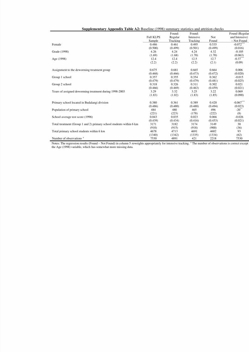
6 After 12 months of tracking, 64% of the Wave 1 sample (2,404 pupils) had been successfully surveyed, refused, orhad died. Among the remaining 1,341 respondents, for budgetary reasons a representative one quarter were“intensively” tracked. As expected, individuals found during the intensive phase were much more likely to be livingoutside of Busia, are somewhat older, and are also less likely to work in agriculture, see supplementary AppendixTable A2. Baird, Hamory and Miguel (2008) has a more detailed discussion of the KLPS tracking approach as wellas its impact on several treatment effect estimates of interest.
collection effort carried out over a decade-long timeframe.7 Reassuringly, tracking rates are nearly
identical in the treatment and control groups.
We have information on where surveyed respondents were living at the time of KLPS-2
survey in 2007-09 (Table 2, Panel B); the locations of residence (for at least four consecutive months
at any point during 1998-2009) are presented in the map in Appendix Figure A2. There is
considerable migration out of Busia District, at nearly 30%, which once again is balanced between
the treatment and control groups. Since the approximately 14% of individuals we did not find, and
thus did not obtain residential information for, are plausibly even more likely to have moved out of
the region, these figures almost certainly understate true out-migration rates. Nearly 8% of
individuals had moved to neighboring districts, including just across the border into the Ugandan
districts of Busia and Bugiri, while 22% of those with location information were living further afield,
with most in Kenya’s major cities of Nairobi, Mombasa or Kisumu. While there are some significant
differences in the migration rates to Nairobi versus Mombasa across the treatment and control
groups, they are relatively minor in magnitude.
We focus on the KLPS-2 data, rather than KLPS-1, in this paper since it was collected at a
more relevant time point for us to assess adult life outcomes: the majority of sample respondents are
adults by 2007-09 (with median age at 22 years as opposed to 18 in KLPS-1), have completed their
schooling, many have married, and a growing share are engaging in wage employment or self-
employment, as shown graphically in Figure 2. While most individuals’ main economic occupation is
farming, as expected in rural Kenya, 16% worked for wages in the last month and 24% at some pointsince 2007, while 11% were currently self-employed outside of farming (Table 2, Panel C). The rates
of wage work and self-employment are nearly identical across the deworming treatment and control
groups, as discussed further below. This pattern simplifies the interpretation of the deworming
earnings impacts we estimate below, although they are somewhat surprising given the large
deworming impacts we estimate on other labor market dimensions, including the large shifts across
employment sectors among wage earners. The issue of selection into the wage earning subsample is
critical for interpretation of the results, and we discuss it extensively below.
3. Deworming impacts on labor market outcomes
This section lays out the estimation and describes deworming impacts on labor outcomes.
7 Other successful recent longitudinal data collection efforts among African youth are described in Beegle et al. (2010) and Lam et al (2008). Pitt, Rosenzweig and Hassan (2011) document high tracking rates in Bangladesh.
The econometric approach relies on the PSDP’s prospective experimental design, namely, the fact
that the program provided individuals in treatment (Group 1 and 2) schools two to three additional
years of deworming treatment. We also adopt the approach in Miguel and Kremer (2004) and
estimate the cross-school externality effects of deworming. Exposure to spillovers is captured by the
number of pupils attending deworming treatment schools within 6 kilometers; conditional on the total
number of primary school pupils within 6 kilometers, the number of treatment pupils is also
determined by the experimental design, generating credible estimates of local spillover impacts.
In the analysis below, the dependent variable is a labor market outcome (such as wage
earnings), Yij,2007-09, for individual i from school j, as measured in the 2007-09 KLPS-2 survey:
(eqn. 2) Yij,2007-09 = a + bT j + Xij,0c + d1N jT + d2N j + eij,2007-09
The labor market outcome is a function of the assigned deworming program treatment status of the
individual’s primary school (T j), a vector Xij,0 of baseline individual and school controls, the number
of treatment school pupils (N jT) and the total number of primary school pupils within 6 km of the
school (N j), and a disturbance term eij,2007-09, which is clustered at the school level.8 The Xij,0 controls
include school geographic and demographic characteristics used in the “list randomization”, the
student gender and grade characteristics used for stratification in drawing the KLPS sample, the pre-
program average school test score to capture school academic quality, as well as controls for the
month and wave of the interview.
The main coefficients of interest are b, which captures any gains accruing to deworming
treatment schools, and d1, which captures any spillover effects of treatment for nearby schools. Bruhn
and McKenzie (2009) argue for including variables used in the randomization procedure as controls
in the analysis, which we do, although as shown below, the coefficient estimates on the treatment
indicator are robust to whether or not the baseline individual and school characteristics are included
as regression controls, as expected given the baseline balance across the treatment and control
groups. Results are also robust to accounting for the cross-school spillovers. In fact, accounting for
externalities tends to increase the b coefficient estimate; in other words, a failure to account for the
program treatment “contamination” generated by spillovers dampens the “naïve” difference between
8 Miguel and Kremer (2004) separately estimate effects of the number of pupils between 0-3 km and 3-6 km. Sincethe analysis in the current paper does not generally find significant differences in externality impacts across thesetwo ranges, we consider the 0-6 km range as a whole for simplicity. The externality results are unchanged if wefocus on the proportion of local primary school pupils who were in treatment schools as the key spillover measure(i.e., N j
T / N j, results not shown). Several additional econometric issues related to estimating externalities arediscussed in Miguel and Kremer (2004).
treatment and control groups (and also potentially leads the researcher to miss a second dimension of
program gains, the spillovers themselves). Certain specifications explore heterogeneity by interacting
individual demographic characteristics with the deworming treatment indicator.
3.2 Deworming Impacts on Labor Earnings, Hours and Wages
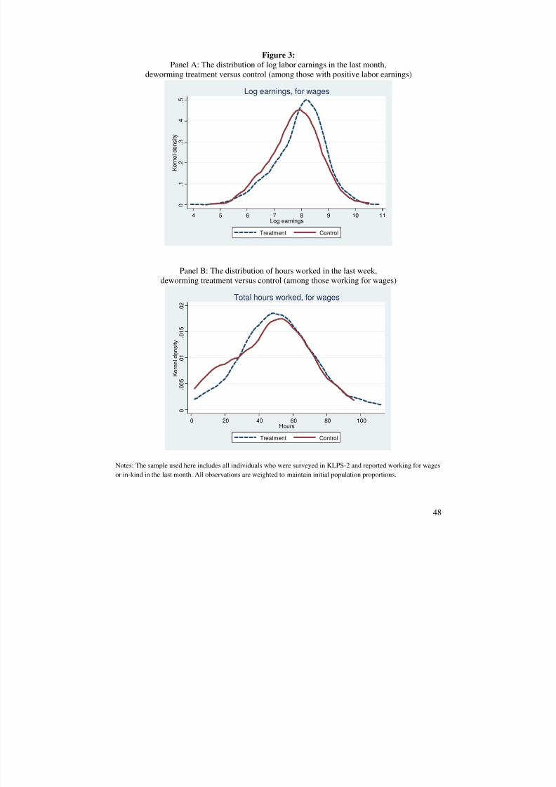
The distribution of wage earnings, as represented in kernel densities, is shifted sharply to the right in
deworming treatment schools (Figure 3, panel A), a first piece of evidence that deworming improved
labor market outcomes. Here and below we present real earnings measures that account for the
higher prices found in the urban areas of Nairobi and Mombasa.9 The distribution of hours worked
for wages or in-kind (among those with at least some wage earnings) is also shifted to the right in the
treatment group (panel B), with a noticeably larger share of treatment individuals working
approximately full-time (roughly 40 hours per week) and fewer working part-time.
We next turn to the regression analysis described above to assess the magnitude and
statistical significance of these effects in Table 3, and find that deworming treatment leads to higher
earnings in: log transformations of earnings (columns 1-3) and linear specifications (columns 4-6);
with and without regression controls; and when cross-school externalities are accounted for. In the
specification without the local externality controls (column 2), the estimated impact is 18.7 log points
(s.e. 7.6, significant at 95% confidence), or roughly 21 percent. In our preferred log specification
with the full set of regression controls (column 3), the impact is 25.3 log points (standard error 9.3,
99% confidence), or approximately 29 percent, a large effect.While the coefficient estimate on the local density of treatment pupils (in thousands) is not
significant at traditional confidence levels (19.9 log points, s.e. 16.8), it reassuringly has the same
sign as the main deworming treatment effect, and a substantial magnitude: an increase of one
standard deviation in the local density of treatment school pupils (917 pupils), which Miguel and
Kremer (2004) found led to large drops in worm infection rates, would boost labor earnings by
We also include an indicator for inclusion in the randomly chosen group of 2001 cost-sharing
schools in all specifications; recall that cost-sharing was associated with much lower deworming
take-up in 2001. Consistent with this drop, the point estimate on the cost-sharing indicator in the
regression shown in Table 3, column 3 is negative and marginally significant at -15.9 log points (s.e.,
8.8). This provides further evidence that deworming treatment is associated with higher earnings.
9 We collected our own comparable price surveys in both rural western Kenya and in urban Nairobi during theadministration of the KLPS-2 surveys, and base the urban price deflator on these data.
The main earnings result is almost unchanged to trimming the top 1% of earners, so the result
is not driven by outliers (Table 4, Panel A). The earnings result is also robust to including a full set of
gender-age fixed effects (estimate 0.270, s.e. 0.093, significant at 99% confidence), to including
fixed effects for each of the “triplets” of Group 1, Group 2 and Group 3 schools from the list
randomization, and considering cross-school cost-sharing externalities (not shown). The next set of
results in Table 4 summarizes a wider set of labor market outcomes among wage earners, using our
preferred specification with the full set of regression controls (as in columns 3 and 6 in Table 3). Log
wages (computed as earnings per hour worked) rise 16.5 log points in the deworming treatment
group, although the effect is not significant at traditional confidence levels (t-stat=1.4), and trimming
the top 1% of wages leads to similar results (not shown).
Positive wage earnings impacts are similar in the larger group of individuals, 24% of the
sample, who have worked for wages at any point since 2007, where we use their most recent monthly
earnings if they are not currently working for wages. The mean impact on log earnings is 0.211 (s.e.
0.072), and there is once again suggestive evidence of positive externality effects (Table 4, Panel B).
Hours worked also increase in the deworming treatment group. Considering the full sample
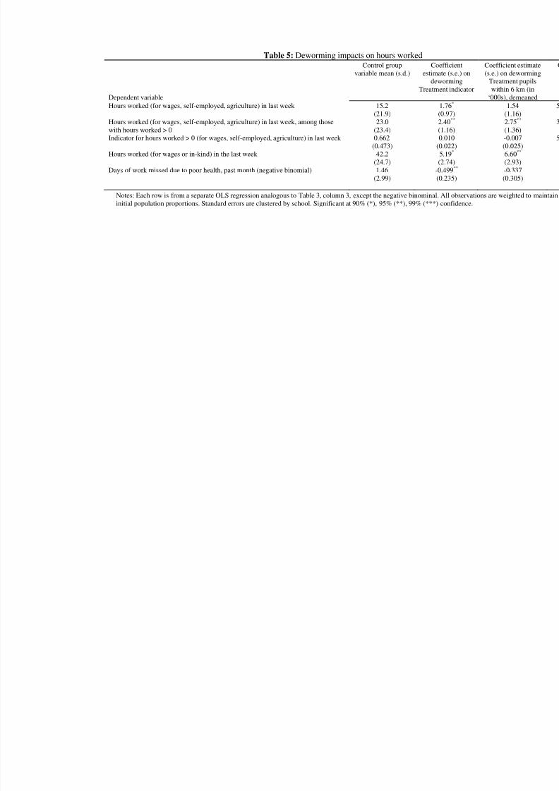
first, hours worked (in any occupation) increased by 1.76 hours (s.e. 0.97, Table 5) on a control
group mean of 15.3 hours, a 12% increase in the full sample that is significant at 90% confidence.
The increase in hours worked is even more pronounced among the 66.2% of the sample that worked
at all in the last week, at 2.40 hours (s.e. 1.16). Note that equal proportions of treatment and control
group individuals worked in the last week, with a small and insignificant difference of just 1.0percentage points between the groups. Hours worked for wages or in-kind in particular increases
substantially in the deworming treatment group by 5.2 hours (significant at 90% confidence), an
increase of 12% on a base of 42.2 hours worked on average in the control group. There is also a
large, positive and significant coefficient estimate on the term capturing local deworming treatment
externalities, at 6.6 (s.e. 2.9). Some of these gains appears to be the direct result of improved health
boosting individual work capacity among wage earners: days lost to poor health in the last month
falls by a third, or 0.499 of a day (s.e. 0.235) in the treatment group.
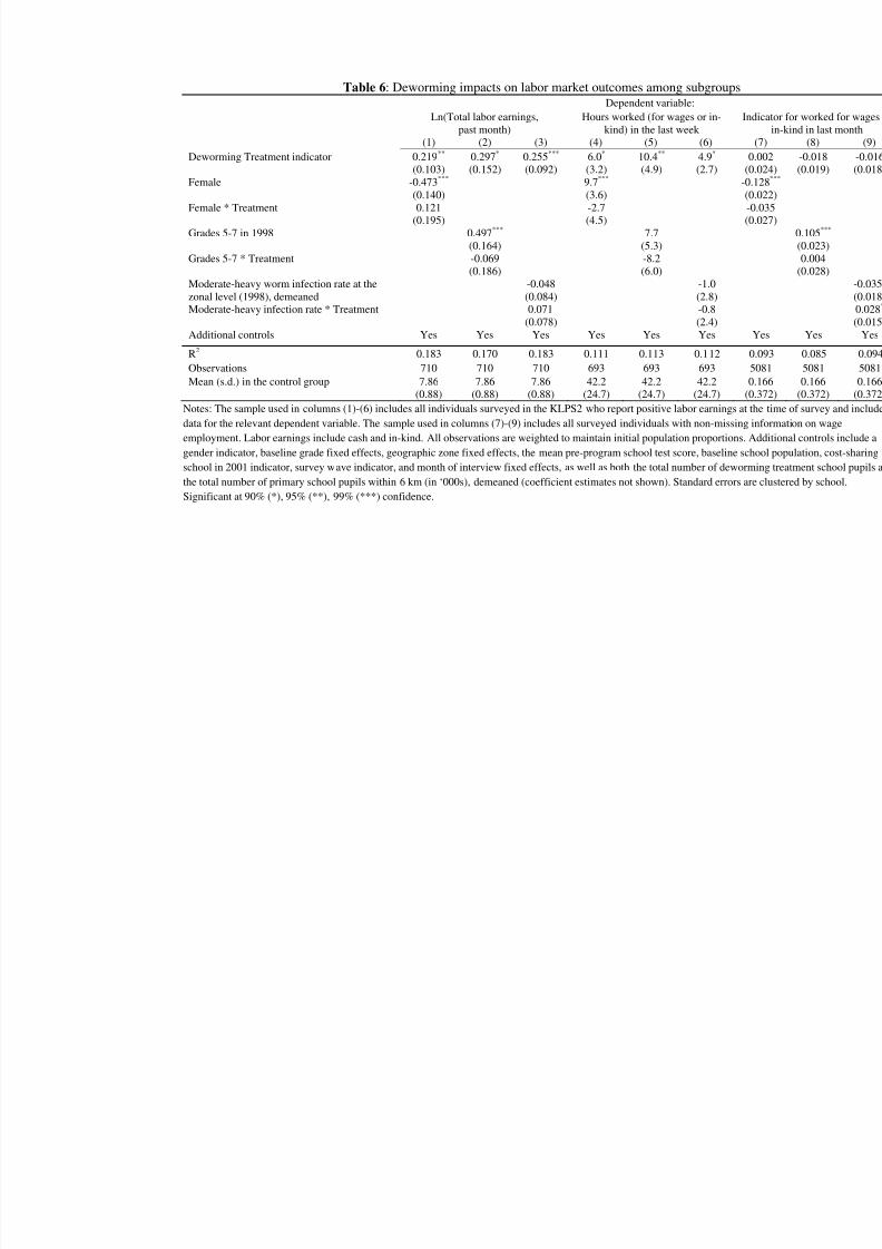
We find no significant evidence that deworming earnings gains differ by gender (Table 6,
column 1), individual age at baseline (column 2) or the local level of serious worm infections at
baseline (column 3). The relatively weak worm infection interaction effect may be due to use of an
average zonal-level baseline worm infection rate, rather than individual-level data (which was not
collected at baseline for the control group for ethical reasons); using zonal averages is likely to
introduce measurement error and attenuation bias. While there is no evidence of differential gender
impacts on hours worked for wages (column 4), it is notable that the gain in work hours is somewhat
higher among individuals who were initially younger at baseline (in grades 2-4), with an average
gain of 10.4 (s.e. 4.9) hours worked, while among those initially in grades 5-7 the effect is positive
but close to zero (column 5). The gains in hours worked are no higher in areas with higher worm
infection rates at baseline (column 6).
3.3 Selection into Wage Earning
The degree of selection into the wage earner subsample is a key issue in assessing the validity of the
earnings results. For example, estimates could be biased downward if deworming led some
individuals with relatively low labor productivity to enter the wage earner sample. While there is no
single ideal solution to this issue, we present several different types of evidence – including
demonstrating that (i) there is no differential selection into wage earning subsamples, (ii) the
observable characteristics of wage earners in the treatment and control groups are indistinguishable,
(iii) there are significant impacts on certain labor market outcomes in the full sample, (iv) results are
robust to a standard Heckman selection correction model, (v) and to restricting analysis to a
subsample where labor market participation is substantially higher than average – all of which
indicate that selection bias is unlikely to be driving our results.
Confirming the result in Table 2, we again find no evidence that deworming treatment
individuals are more likely to be working for wages or in-kind in the last month (Table 4, Panel A,
estimate -0.015, s.e. 0.018), making it less likely that differential selection is driving the results.There is similarly no differential selection into the subsample who have worked for wages at any
point since 2007 by treatment group (Panel B, estimate 0.000, s.e. 0.021). While it remains possible
that deworming led certain types of individuals to enter wage earning and others to leave while
leaving the overall proportions unchanged, the lack of deworming impacts on the proportion of
individuals working in both self-employed and agriculture as well makes this appear even less likely.
We further confirm that there is no differential selection into the wage earner sample by
gender (Table 6, column 7) or age (column 8). There is some evidence of greater selection into the
wage earner subsample among deworming treatment individuals in zones with high worm infection
rates at baseline (column 9), but the coefficient is only marginally significant and its magnitude is
quite small. To illustrate, a one standard deviation increase in the baseline local moderate-heavy
worm infection rate is 0.2, and thus an increase of this magnitude leads to a (0.2) x (0.028) = 0.0056
increase in the likelihood that individuals are wage earners, a small 3.4 percent increase on the base
of 0.166 in the control group. Baseline characteristics, including academic performance measures,
attempt to disentangle individuals’ separate contributions. As a result, we focus on a set of standard
but imperfect proxies in this subsection.
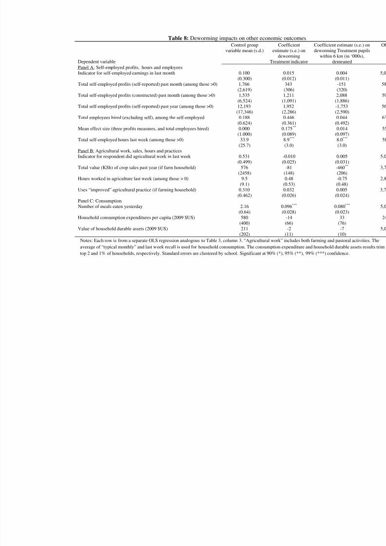
Business outcomes improved considerably among the self-employed. The estimated
deworming treatment effect on the profits of the self-employed (as directly reported in the survey) is
positive (343 Shillings, s.e. 306, Panel A), although this 19% gain is not significant at traditional
confidence levels, and there are similarly positive but not significant impacts on reported profits in
the last year, on a profit measure based directly on revenues and expenses reported in the survey, as
well as on the total number of employees hired (0.446, s.e. 0.361). The mean effect size of the three
profit measures and the total employees hired taken together is positive, relatively large and
statistically significant at 95% confidence at 0.175 (s.e., 0.089), where the magnitude is interpretable
as 0.175 standard deviations of the normalized control group distribution, a sizeable effect.
There is also a large increase in hours worked among the self-employed, with a gain of 8.9
hours (s.e. 3.0) on a base of 33.9 hours worked on average in the control group, a 26% increase.
There is also a large externality effect on self-employed hours worked (8.0, s.e. 3.0), further
indication that deworming appears to boost work hours.
Among the majority of the total sample that continues to work primarily on their own farm
(rather than for wages or as self-employed), there is no indication that deworming led to higher crop
sales in the past year, greater hours worked in agriculture in the last week, or to higher adoption of
“improved” agricultural practices including fertilizer, hybrid seeds or irrigation (Table 8, Panel B).
The failure to find increased crop sales may, in part, be due to the fact that households are consumingmore grain of the grain they produced, as suggested by the increase in meals eaten. Again, these
results should be read with a grain of salt as we are unable to credibly measure individual on-farm
productivity, but taken together, there are no clear impacts on agricultural outcomes we can measure.
3.6 Impacts on consumption
Household consumption expenditures are a standard tool for assessing living standards in rural areas
of less developed countries, where much of the population engages in subsistence agriculture rather
than wage work. One consumption measure, the number of meals consumed by the respondent
yesterday, is narrower than total consumption expenditures but has the advantage that it was
collected for the entire sample. Deworming treatment individuals consume 0.096 more meals (s.e.
0.028, significant at 99% confidence, Panel C) than the control group, and the externality impact is
also large and positive (0.080, s.e. 0.023, 99% confidence). This suggests that deworming led to
A standard LSMS-style consumption expenditure module was collected for roughly 5% of
the KLPS-2 sample during 2007-09, for a total of 254 complete surveys. Such surveys are time-
consuming and project budget constraints prevented us from collected a larger number of surveys.
Note, too, that such data faces an important limitation in practice since consumption expenditures are
best captured at the household level, and thus any productivity gains among KLPS respondents
would be “diluted” if other household members do not experience similar gains, making them more
difficult to detect in per capita household consumption measures. The data indicate that per capita
average consumption levels in the control group are reasonable for rural Kenya, at US$580 (in
exchange rate terms, Table 8, Panel C), and that food constitutes roughly 64% of total consumption.
The estimated treatment effect for total consumption is near zero and not statistically significant at
traditional confidence levels (-$14, s.e. $66), though it is worth noting that the confidence interval is
quite large and includes large gains. The estimated deworming effect on a wealth measure, total
household durable asset ownership, is also close to zero and not significant at traditional levels.
Thus taken together, there is some suggestive evidence that deworming improved living
standards in the full sample as captured by meals eaten, with the important caveat that impacts on a
broader consumption measure are unfortunately quite imprecisely estimated.
4. Deworming impacts on education and health
We first work through the comparative statics of a simple textbook model of health, educational
investment and income to illustrate the channels through which deworming is likely to affect labormarket outcomes (in subsection 4.1), and then estimate deworming impacts along educational (4.2)
and health (4.3) dimensions.
4.1 Understanding the impact of health gains on educational investments and lifetime income
While many existing studies focus on educational attainment as the most likely channel linking child
health gains to higher adult earnings, Bleakley (2010) rightly points out that standard models do not
necessarily imply that education is the key mechanism. In this sub-section, we present a simple
model related to Bleakley’s to illustrate this point and generate further hypotheses.
We consider a model in which individuals choose how much education (denoted e below) to
obtain to maximize discounted lifetime earnings, y, and examine how these schooling investments
change as a function of child health (denoted h). The discounted future income benefits to schooling
are b(e,h), and the costs (including both direct tuition costs and the opportunity cost of time spent in
school rather than working) are c(e,h). Both the benefits and costs are increasing in education and
Miguel and Kremer (2004) found large schoolattendance gains among deworming treatment pupils, especially among younger children.
In assessing the welfare impacts of increased adult earnings, a further application of the
envelope theorem would imply that these are best captured in wage (productivity) gains rather than in
increased hours worked. However, this only holds if individuals with poor health are already at or
near their optimal labor supply. To the extent that they are not, and better health improves the
capacity to work longer hours, then the total gain in earnings (rather than just gains generated by
higher wages per hour worked) is a more appropriate welfare metric; we return to this issue in section
5 below in our discussion of the returns to deworming investment.11 The seminal model of health
capital developed in Grossman (1972) argues that the fundamental difference between health capital
and other forms of human capital, such as those created through education, is precisely the fact that
10 Bleakley (2010) makes a similar observation about child school attendance gains. In the framework laid outabove, this attendance effect is consistent with either the health investment allowing children to avoid somesickness-induced absenteeism, or with deworming shifting the marginal benefits of education more than themarginal costs (beh > ceh). An alternative explanation for suboptimal educational investment could be agencyproblems or imperfect altruism within the household that leads parents to place too little weight on future child labormarket gains from education. Note that in such a setting, improving child health (and thus labor productivity) today
might instead boost current school drop-out rates.11 The relevant expression is
dh
dL
L
u
h
u
dh
du
L L
*
**
*
,
where L denotes hours worked and u is individual utility, in the context of a model where individuals face a labor-
leisure trade-off. To the extent that individuals in poor health are working the optimal number of hours (L*) then the
second term equals zero, implying that increased hours worked should not be considered in assessing the welfare
gains from better health, but this does not hold if poor health constrains labor supply below L*.
better health status increases “the total amount of time [one] can spend producing money earnings
and commodities” (p. 224). It is worth noting that the increases in adult hours worked and reduction
in work days lost due to sickness (Table 5) among deworming treatment individuals, reported above
are consistent with the view that healthier adults have greater work capacity and are thus better able
to attain their ideal labor supply, leading to first-order welfare gains.
4.2 Impacts on education
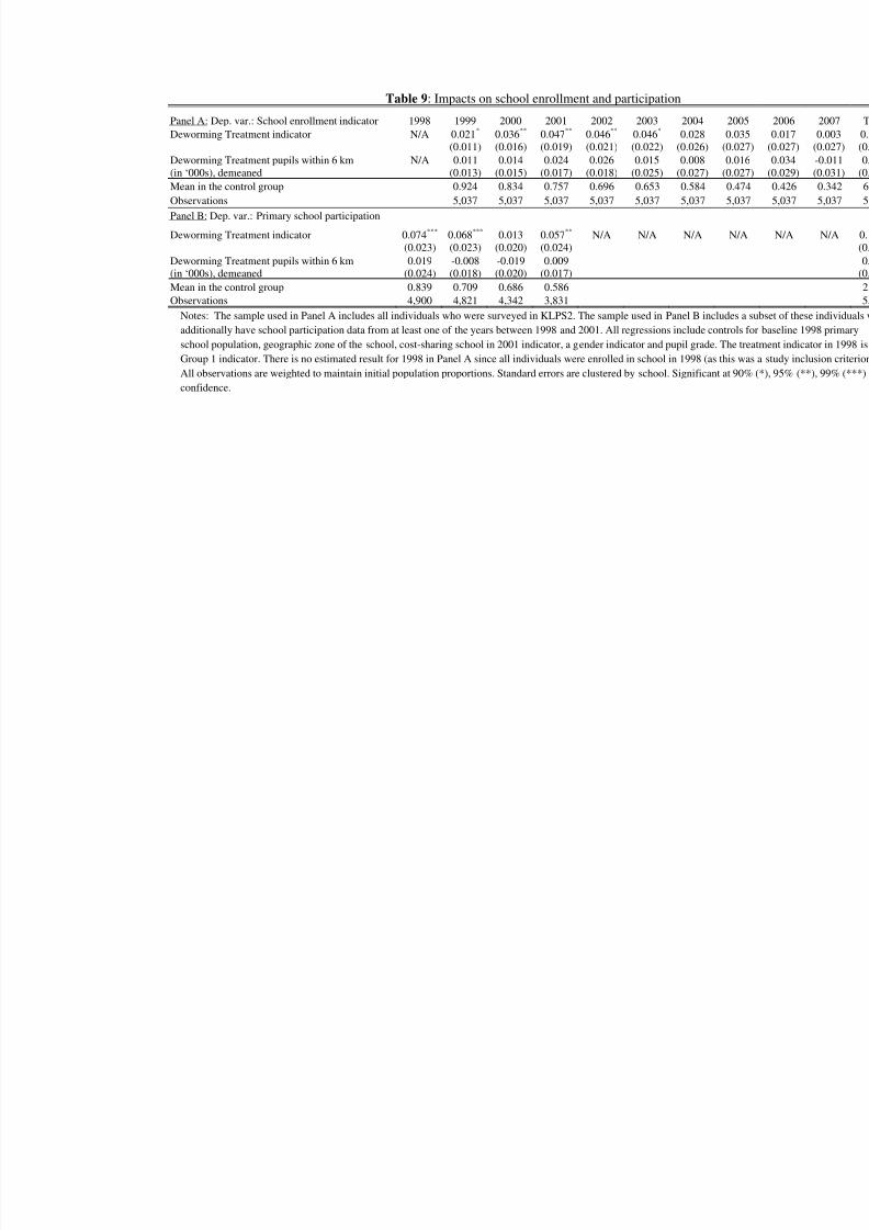
We examine school enrollment and attendance using two different data sources in Table 9. In Panel
A, the dependent variable is school enrollment as reported by the respondent in the KLPS-2 survey,
which equals one if the individual was enrolled for at least part of a given year. These show
consistently positive effects from 1999 to 2007 both on the deworming treatment indicator and the
externalities term, and the total increase in school enrollment in treatment relative to control schools
over the period is 0.279 years (s.e. 0.147, significant at 90% confidence). Note that there is no
treatment effect estimate for 1998 since all students were enrolled at some point in 1998, as a
criterion for inclusion in the KLPS sample. The treatment effect estimates are largest during 1999-
2003 before tailing off during 2004-07, as predicted in the optimal educational investment
framework above since the current opportunity cost of time is rising relative to the later benefits of
schooling as individuals age.
The data in Panel B is school participation, namely, being found present in school by survey
enumerators on the day of an unannounced school attendance check. This is our most objectivemeasure of actual time spent at school, and was a main outcome measure in Miguel and Kremer
(2004). The enrollment measure in Panel A misses much of the attendance variation captured in this
measure. However, two important limitations of the school participation data are that it was only
collected during 1998-2001, and only at primary schools in the study area; the falling sample size
between 1998 to 2001 is mainly driven by students graduating from primary school. School
participation rates also rise significantly in the deworming treatment group, by 0.074 (s.e. 0.023) and
0.068 (s.e. 0.023) in 1998 and 1999, respectively, before dropping off somewhat in later years
(particularly in 2000). Total school participation gains are 0.129 of a year of schooling (s.e. 0.064,
significant at 95% confidence). Given that the school enrollment data misses out on attendance
impacts, which are sizeable, a plausible lower bound on the total increase in time spent in school
induced by the deworming intervention is the 0.129 gain in school participation from 1998-2001 plus
the school enrollment gains from 2002-2007, which works out to 0.304 years of schooling.12
Despite the sizeable gains in years of school enrollment, there are no significant impacts on
either total grades of schooling completed (0.153, s.e. 0.143 – Table 10, Panel A) or attending at least
some secondary school (0.032, s.e. 0.035), although note that both of these point estimates are
positive. The likely explanation is that the increased years in school are accompanied by increased
grade repetition (0.060, s.e. 0.017, significant at 99% confidence). To summarize, deworming
treatment individuals attended school more and were enrolled for more years on average, but do not
attain significantly more grades in part because repetition rates rise substantially.
Test score performance is another natural way to assess deworming impacts on human capital
and skills. While the impact of deworming on primary school academic test score performance in
1999 is positive but not statistically significant (Table 10, Panel B), there is suggestive evidence that
the passing rate did improve on the key primary school graduation exam, the Kenya Certificate of
Primary Education (point estimate 0.046, s.e. 0.031). There is also some evidence that English
vocabulary knowledge (collected during the 2007-09 survey) is somewhat higher in the deworming
treatment group (impact of 0.076 standard deviations in a normalized distribution, s.e., 0.055). The
mean effect size of the 1999 test score, the indicator for passing the primary school leaving exam,
and the English vocabulary score in 2007-09 taken together does yield a normalized point estimate of
0.112 that is statistically significant at 90% confidence (s.e. 0.067), providing suggestive evidence of
moderate human capital gains in the treatment group.As expected, there is no effect on the Raven’s Matrices cognitive exam, which is designed to
capture general intelligence rather than acquired skills (Panel B). While many would argue that
nutritional gains in the first few years of life could in fact generate improved cognitive functioning as
captured in a Raven’s exam – as Ozier (2010) indeed does find among younger siblings of the
deworming beneficiaries – it was apparently already “too late” for such gains among the primary
school age children in our study.
4.3 Impacts on health and nutrition
There is evidence that adult health also improved as a result of deworming. Respondent self-reported
health (on a normalized 0 to 1 scale) improved by 0.041 (s.e. 0.018, significant at 95% confidence,
Table 11, panel A). Many studies have found that self-reported health reliably predicts actual
12 The impacts of deworming on years enrolled in school are somewhat larger in the wage earner subsample, thoughwe cannot reject the hypothesis that effects are the same for this subgroup as for the full sample (not shown).
morbidity and mortality even when other known health risk factors are accounted for (Idler and
Benyamini 1997, Haddock et al. 2006, Brook et al. 1984). Note that it is somewhat difficult to
interpret this impact causally since it may partially reflect health gains driven by the higher adult
earnings detailed above, in addition to the direct health benefits of earlier deworming. Yet the fact
that there were similar positive and statistically significant impacts on self-reported health in earlier
periods, namely, in surveys administered in 1999 before most in sample individuals were working
(see Table 11, panel C and Miguel and Kremer 2004), suggests that at least part of the effect is
directly due to deworming.
In terms of other health outcomes, there is no evidence that deworming improved self-
reported happiness or wellbeing or reduced major health shocks. Total health expenditures by the
respondent in the last month are significantly higher in the treatment group (91.1 Shillings, s.e. 30.0),
suggesting that they may have greater ability or willingness to make health investments, but
interpretation is again complicated by the fact that such spending also reflects health needs. Despite
the finding that the number of meals consumed is larger for deworming treatment individuals (in
Table 8), deworming did not lead to higher body mass index (Table 11, Panel B). Nor are there
detectable height gains, and these non-impacts hold even when we restrict attention to younger
individuals (those in grades 2-4 in 1998, regression not shown).
It is difficult to disentangle the precise contributions of the education versus health gains we
document in driving deworming’s impact on labor market earnings, as the causal impacts on earnings
of schooling attainment, other measures of skill (like our test of English vocabulary), self-reportedhealth and our other measures are themselves not very well-understood, and interactions among these
channels are also possible. We are able to show in the cross-section, however, that the education and
health factors we focus on are correlated with higher earnings among the control group. For instance,
a Mincerian regression indicates that the return to a year of schooling is between 6 to 12 log points
(and highly significant, not shown), and both academic test scores and self-reported health are also
associated with higher earnings. At a minimum, these associations establish as plausible the claim
that the education and health channels that we focus on are contributing to higher earnings in the
deworming treatment group.
The growing evidence that deworming improves immunological resistance to other
infections, such as malaria (i.e., Kirwan et al. 2010), also implies that deworming might generate
health benefits beyond those captured solely in anthropometric measures. Fortunately, we are able to
assess the claim about malaria with the data from the original deworming program, in particular, a
1999 survey conducted among a representative subsample of pupils. To use our standard econometric
community-wide benefits to deworming among those not of school age, for example, among the
younger siblings of the treated.13
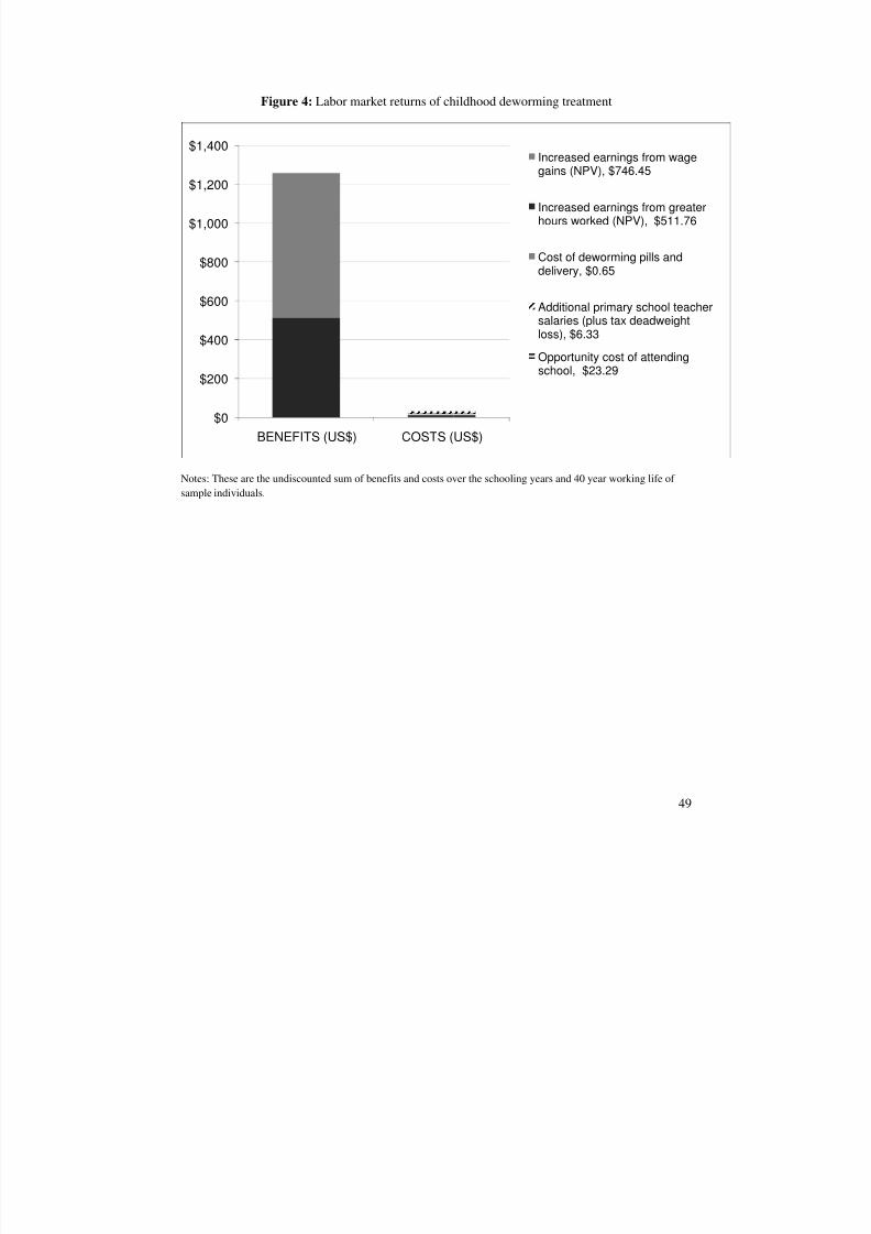
Under these assumptions, the average gain in total lifetime earnings (undiscounted) from
deworming treatment is $1,258 (Table 12, Panel A). Note that the externality benefits to deworming
treatment could also be very large (at $2,213 per 1000 additional treatment pupils within 6 km, which
is roughly equivalent to an increase of one standard deviation in this density, result not shown), and
would thus substantially boost the rates of return reported below.
We next derive an estimate of benefits only considering higher wages (earnings per hour),
ignoring the greater number of hours worked by deworming treatment group individuals. As
discussed above, the implicit assumption made when focusing only on wage gains in assessing
welfare is that control group individuals are near their optimal labor supply level, and thus the greater
hours worked by the treatment group will, to a first order approximation, have zero utility benefits. In
contrast, if better health allows individuals to attain something closer to their optimal labor supply by
reducing undesired illness-induced absenteeism and increasing work capacity, then the additional
hours worked can legitimately be considered welfare gains. The true welfare gains thus probably lie
in between the gains derived from focusing on total earnings versus wages alone. Focusing on wage
gains alone, the lifetime benefits are $746.
There are three main social costs to deworming. The most obvious is the direct cost of
deworming pill purchase and delivery through the schools. We use current estimates of per pupil
mass treatment costs (provided by the NGO DewormTheWorld) of $0.59 per year. This costincorporates the time of personnel needed to administer drugs through a mass school-based program,
and accounts for the fraction of our sample that requires treatment with the more expensive drug for
schistosomiasis (praziquantel). The total direct deworming cost then is the 2.41 years of additional
deworming in the treatment group times $0.59, times the drug compliance rate in treatment schools,
or $0.65 (Table 12, Panel B).
The second component is the opportunity cost of time spent in school rather than doing
something else, presumably working. We calculate the maximum number of potential extra work
days that children could gain (given the long school vacation periods in Kenyan schools), namely
185 days. We then compute the increased school participation (for 1998-2001, years where this data
is available) and school enrollment (for 2002-2007) among treatment school individuals, at each
individual age (in an analysis similar to Table 9); we disaggregate effects by child age since
13 Ozier (2010) shows that children 0-3 years old when the deworming program was launched who had oldersiblings in treatment schools themselves show large nutritional and cognitive gains ten years later.
schooling gains are often concentrated among younger children. We then use recent data on the
average unskilled agricultural wage in western Kenya (reported in Suri 2009), at $1.26 per day, as a
benchmark. We assume that out-of-school children work approximately 20 more hours per week than
those enrolled in school, which is conservative given recent time-use survey data from sub-Saharan
Africa (Bardasi and Wodon 2006, Akabayashi and Psacharopoulos 1999). Finally, we make the
assumption that foregone wage earnings would be zero for children at age 8 and would increase
linearly up to 100% of the local unskilled wage for 18 year olds. This implies that, say, 13 year olds
are roughly half as productive as adults per hour worked.
While some of these assumptions are difficult to validate given the well-known difficulties in
measuring both agricultural and home productivity, and the particular rarity of such data for children,
we feel these are likely to be conservative (and in any case, the returns to deworming remain large
with even more conservative assumptions). The average per capita opportunity cost of time generated
by deworming treatment under these assumptions is $23.29.
The third main social cost would be incurred if governments responded to the increased
school participation induced by the deworming program by hiring more teachers, in order to maintain
class sizes at the same average level as before the program. This would necessitate increasing the
number of teachers by the same proportion as the rise in school participation. To compute these
costs we employ official data on current Kenyan primary school and secondary school teacher
salaries, and also assume that a deadweight loss of 20% would be incurred on the government
revenue raised to fund this expansion (Auriol and Walters 2009).14
The total social cost (includingthe deadweight loss) of hiring a sufficient number of teachers is thus $6.33 per treatment individual.
A graphical depiction of these various benefits and costs is presented in Figure 4. It is
immediate that the undiscounted lifetime benefits of deworming far outweigh the costs, even when
just considering the income gains that result from higher wages alone. The results are also presented
in Table 12, Panel C, both for the total earnings case, where the ratio of benefits to costs is 41.6, and
for wages alone it is 24.7.
These estimates ignore the externality benefits of deworming treatment among those located
within 6 kilometers of treatment schools. While estimated externality effects (Table 3) are not
significant at traditional confidence levels, if we take their magnitude seriously and consider
productivity (wage) gains, the externality benefits of deworming alone outweigh the costs (of drug
14 Busia District Education Office statistics indicate that average total primary school teacher annual compensationis $2,861 and average secondary school compensation is $4,060.
delivery and the opportunity cost of child time) by a ratio of 5.84:1. These gains might justify full
public subsidies for deworming treatment.
We have so far focused on wage earners because their productivity gains are much more
accurately measured than those working in self-employment or agriculture. If we were to abandon
the assumption that earnings and wage gains were only experienced by those with wage earnings,
and assumed that the full sample experienced analogous living standard gains, then the social benefit-
cost ratio for deworming investment would be massive: 245.9 for the returns in terms of earnings and
145.9 in terms of wage productivity. While it is impossible for us to accurately assess just how much
productivity did increase for those not working for wages given our data, the point here is that any
living standards gains among the non-wage earning group would drastically increase the social
returns to deworming investments.
An alternative approach to comparing the future benefits and costs of an investment is by
calculating its internal rate of return (IRR). The IRR for deworming when we consider total earnings
is 22.1% per annum, and it is 17.7% when we focus on wage productivity gains alone (Table 12,
Panel D). Once again, these are quite high returns. The interpretation is that a social planner with an
annual discount rate or cost of capital of less than 22.1% would choose to invest in deworming as a
human capital investment. As a point of reference, at the time of writing, nominal commercial
interest rates in Kenya are 10-12% per annum, the rate on long-term sovereign debt is 11% and
inflation is 3% (according to the Central Bank of Kenya website).15 Thus deworming appears to be
an attractive investment given the real cost of capital in Kenya.16
6. Conclusion
We exploit an unusually useful setting for estimating the impact of child health gains on adult
earnings and other life outcomes. The Kenya Primary School Deworming Program was
experimentally phased-in across 75 rural schools between 1998 and 2001 in a region with high rates
of intestinal worm infections, one of the world’s most widespread diseases, especially among
15 This figure was obtained at: http://www.centralbank.go.ke/ (accessed November 1, 2010). Note that the analogousinternal rate of return for the Indonesia primary school construction program studied in Duflo (2001) was 4 to 10%.16 A fuller social benefit-cost calculation would consider general equilibrium effects in the labor market of boostingproductivity among younger cohorts, for instance, on the outcomes of older cohorts. The general equilibrium effectswill depend on the degree and speed of aggregate physical capital accumulation in response to human capital gains(Duflo 2004), as well as the magnitude of any positive human capital spillovers across neighbors and coworkers(Moretti 2004, Mas and Moretti 2009). Duflo (2004) finds mixed impacts on the cohorts too old to have directlybenefited from the 1970’s school construction program in Indonesia, with positive gains in labor marketparticipation but some moderate drops in wages among those working.
children in poor countries. As a result the treatment group exogenously received an average of two to
three more years of deworming treatment than the control group. A representative subset of the
sample was followed up for roughly a decade, through 2007-09 in the Kenya Life Panel Survey, with
high survey tracking rates, and the labor market outcomes of the treatment and control groups are
compared to assess impacts.
Among those working for wages, average adult earnings rise by approximately 21 to 29% as
a result of deworming. These gains are accompanied by large increases in average hours worked (by
12%), a reduction in work days lost to sickness, and sharp shifts in employment towards high-paying
manufacturing sector jobs (especially for males) and away from casual labor and domestic services
employment (for females). The finding that shifts into different employment sectors account for the
bulk of the earnings gains suggests that characteristics of the broader labor market – for instance,
sufficient demand for manufacturing workers – may be critical for translating better health into
higher living standards. While a simple model of optimal educational investment gives ambiguous
predictions about the relative roles played by education versus health channels, there are significant
deworming impacts on total years of school enrollment, test scores and self-reported health,
suggesting that both may be important. The social returns to child deworming treatment are very
high, with conservative estimates of the benefit-cost ratio ranging from 24.7 to 41.6.
These findings build on and complement Bleakley’s work on historical deworming programs
in the U.S. South in the early 20th century. It is remarkable that his estimated earnings gains in the
U.S. South line up so closely with our findings: while Bleakley’s (2007a) U.S. estimates imply thatthe treatment of worm infections at rates commonly found in Africa would raise earnings by 24%, we
estimate gains of 21 to 29%. The correspondence between these two sets of results – using distinct
research designs and data from different time periods – increases confidence in the external validity
of both findings.
The main implication of this paper is that childhood health investments like school-based
deworming can substantially boost adult earnings. It goes without saying that deworming alone, and
its associated increase in earnings, cannot make more than a small dent in the large gap in living
standards between poor African countries like Kenya and the world’s rich countries. Yet that obvious
point does not make deworming any less attractive as a public policy option given its extraordinarily
high social rates of return, and the fact that boosting income by one quarter would have major
welfare impacts for households living near subsistence.
Aghion, Philippe, Peter Howitt, and Fabrice Murtin. (2010). “The Relationship between Health andGrowth: When Lucas Meets Nelson-Phelps”, forthcoming Review of Economics and
Institutions.Akabayashi, Hideo, and George Psacharopoulos. (1999). “The trade-off between child labour and
human capital formation: A Tanzanian case study”, Journal of Development Studies, 35(5),120-140.
Alderman, Harold, John Hoddinott, Bill Kinsey. (2006a). "Long-term consequences of earlychildhood malnutrition," Oxford Economic Papers 58, 450-474.
Alderman, Harold, J. Konde-Lule, I. Sebuliba, D. Bundy, A. Hall. (2006b). “Increased weight gain inpreschool children due to mass albendazole treatment given during ‘Child Health Days’ inUganda: A cluster randomized controlled trial”, British Medical Journal, 333, 122-126.
Alderman, Harold. (2007). “Improving nutrition through community growth promotion: Longitudinalstudy of nutrition and early child development program in Uganda”, World Development ,35(8), 1376-1389.
Almond, Douglas (2006). “Is the 1918 Influenza Pandemic Over? Long-Term Effects of In Utero Influenza Exposure in the Post-1940 U.S. Population”. Journal of Political Economy, Vol.
144(4): 672-712.Almond, Douglas and Bhashkar Mazumder (2008). “Health Capital and the Prenatal Environment:
The Effect of Maternal Fasting during Pregnancy”, NBER WP#14428.Auriol, Emmanuelle, and Michael Walters. (2009). “The Marginal Cost of Public Funds and Tax
Reform in Africa”, unpublished working paper, University of Toulouse.Baird, Sarah, Joan Hamory, and Edward Miguel. (2008) “Attrition and Migration in the Kenya Life
Panel Survey.” University of California, Berkeley CIDER Working Paper.Bardasi, Elena, and Quentin Wodon. (2006). “Measuring time poverty and analyzing its
determinants: Concepts and application to Guinea (Chapter 4)”, in C. Mark Blackden andQuentin Wodon (eds.), Gender, Time Use, and Poverty in Sub-Saharan Africa. WorkingPaper #73. World Bank, Washington DC.
Beegle, K., J. De Weerdt, S. Dercon. (2010). “Migration and Economic Mobility in Tanzania:
Evidence from a Tracking Survey”, forthcoming Review of Economics and Statistics.Behrman, Jere. (1996). “The Impact of Health and Nutrition on Education,” World Bank Research
Observer , vol. 11(1), 23-37.Behrman, Jere R., Maria Cecilia Calderon, Samuel Preston, John Hoddinott, Reynaldo Martorell and
Aryeh D. Stein. (2009). “Nutritional Supplementation of Girls Influences the Growth of theirChildren: Prospective Study in Guatemala”, American Journal of Clinical Nutrition, 90(November), 1372-1379.
Bleakley, Hoyt. (2007a). “Disease and Development: Evidence from Hookworm Eradication in theAmerican South.” Quarterly Journal of Economics, 122(1):73-117.
Bleakley, Hoyt. (2007b). “Spillovers and aggregate effects of health capital: evidence fromcampaigns against parasitic disease in the Americas”, working paper Univ. of Chicago.
Bleakley, Hoyt. (2010). “Health, Human Capital, and Development”. Annual Review of Economics, 2, 283-310.Brook, Robert H., John E. Ware, William H. Rogers, Emmett B. Keeler, Allyson Ross Davies, Cathy
D. Sherbourne, George A. Goldberg, Kathleen N. Lohr, Patricia Camp, Joseph P. Newhouse.(1984). The Effect of Coinsurance on the Health of Adults: Results from the RAND Health
Insurance Experiment . RAND Corporation: Santa Monica, CA.Brooker, S., Miguel, E.A., Moulin, S., Luoba, A.I., Bundy, D.A.P. and Kremer, M. (2000a).
“Epidemiology of Single and Multiple Species Helminth Infections among Schoolchildren inBusia District, Kenya”, East African Medical Journal, 77, 157-161.
Brooker, Simon, Megan Rowlands, Laurence Haller, Lorenzo Savioli, and Donald Bundy. (2000b)“Towards an Atlas of Helminth Infection in Sub-Saharan Africa: The Use of GeographicalInformation Systems (GIS)”, Parasitology Today, 16(7), 303-307.
Bruhn, Miriam and David McKenzie. (2009). “In pursuit of balance: Randomization in practice indevelopment field experiments”, American Economic Journal: Applied Economics, 1(4),200-232.
Bundy, D.A.P. (1994). “The Global Burden of Intestinal Nematode Disease.” Transactions of the
Royal Society of Tropical Medicine and Hygiene, 88, 259-261.Bundy, Donald A.P., Michael Kremer, Hoyt Bleakley, Matthew C.H. Jukes, and Edward Miguel.
(2009). “Deworming and development: Asking the right questions, asking the questionsright”, PLoS Neglected Tropical Diseases, 3(1): e362. doi:10.1371/journal.pntd.0000362.
Case, Anne, and Christina Paxson. (2010). “Causes and Consequences of Early Life Health”, Demography, 47 (Supplement), S65-S85.
Chattopadhyay, Raghabendra, and Esther Duflo. (2004). “Women as policymakers: Evidence from arandomized policy experiment in India”, Econometrica, 75(2), 1409-1443.
Conley, Dalton and Neil G. Bennett. (2000). “Is Biology Destiny? Birth Weight and Life Chances”, American Sociological Review, 65(3), 458-467.
Currie, Janet, and Duncan Thomas. (1995). “Does Head Start Make A Difference?”, American Economic Review, 85(3), 341-364.
Currie, Janet, Eliana Garces, and Duncan Thomas. (2002). “Longer Term Effects of Head Start”, American Economic Review, 92(4), 999-1012.
de Silva, NR, Brooker S, Hotez PJ, Montresor A, Engels D, Savioli L. (2003). “Soil-transmittedhelminth infections: updating the global picture” Trends in Parasitology, 19(12):547-51.
de Silva, N.R., Chan, M.S., and D.A.P. Bundy (1997). “Morbidity and Mortality Due to Ascariasis:Re-estimation and Sensitivity Analysis of Global Numbers at Risk.” Tropical Medicine and
International Health , 2(6):519-28.Deaton, Angus. (2010). “Instruments, Randomization and Learning about Development”, Journal of
Economic Literature, 48, 424-455.Duflo, Esther. (2001). “Schooling and labor market consequences of school construction in
Indonesia: Evidence from an unusual policy experiment”, American Economic Review,
91(4), 795-813.Duflo, Esther. (2004). “The medium-run effects of educational expansion: Evidence from a large
school construction program in Indonesia”, J. of Development Economics, 74(1), 163-97.Fernald, Lia C. and Sally M. Grantham-McGregor. (1998). “Stress response in school-age children
who have been growth retarded since early childhood.” American Journal of Clinical
Nutrition, 68(3), 691-698.Field, Erica, Omar Robles, and Maximo Torero. (2009). “Iodine Deficiency and Schooling
attainment in Tanzania.” American Economic Journal: Applied Economics, 1(4): 140-69.Fincham, John E., M.B.Markus, and V.J. Adams. (2003). “Could control of soil-transmitted
helminthic infection influence the HIV/AIDS pandemic?”, Acta Tropica, 86(2-3), 315-333.
Glewwe, Paul, Hanan G. Jacoby, Elizabeth M. King (2001). “Early childhood nutrition and academicachievement: a longitudinal analysis.” J. of Public Economics, 81: 345-368.
Grossman, Michael. (1972). “On the Concept of Health Capital and the Demand for Health”, Journal
of Political Economy, 80(2), 223-255.Guyatt, H.L., Brooker, S., Kihamia, C.M., Hall, A. & Bundy, D.A. 2001, "Evaluation of efficacy of
school-based anthelmintic treatments against anaemia in children in the United Republic of Tanzania", Bulletin of the World Health Organization, 79(8), 695-703.
Haddock, Christopher K., Walker S.C. Poston, Sara A. Pyle, Robert C. Klesges, Mark W. VanderWeg, Alan Peterson, Margaret Debon. (2006). “The validity of self-rated health as a measureof health status among young military personnel: evidence from a cross-sectional survey”, Health and Quality of Life Outcomes, 4(57).
Heckman, James. (1979). “Sample selection bias as a specification error”, Econometrica, 47, 153-61.Hoddinott, John, John A. Maluccio, Jere R Behrman, Rafael Flores and Reynaldo Martorell. (2008).
“The Impact of Nutrition During Early Childhood on Income, Hours Worked, and Wages of Guatemalan Adults”, Lancet , 371 (February), 411-416.
Hotez, P.J. & Ferris, M.T. (2006), "The antipoverty vaccines", Vaccine, 24(31-32), 5787-5799.Idler, Ellen L., and Yael Benyamini. (1997). “Self-rated health and mortality: A review of twenty-
seven community studies”, Journal of Health and Social Behavior , 38(1), 21-37.Jukes, Matthew C. H, Margaret Pinder, Elena L. Grigorenko, Helen Baños Smith, Gijs Walraven,
Elisa Meier Bariau, Robert J. Sternberg, Lesley J. Drake et al. (2006). “Long-Term Impact of Malaria Chemoprophylaxis on Cognitive Abilities and Educational Attainment: Follow-Upof a Controlled Trial.” PLoS Clinical Trials, 1(4): e19.
Jukes, Matthew C. H., Lesley J. Drake, and Donald A. P. Bundy. School Health, Nutrition, And
Education for All: Levelling the Playing Field. CABI Publishing, Wallingford 2007.
Kirwan, P., Jackson, A.L., Asaolu, S.O., Molloy, S.F., Abiona, T.C., Bruce, M.C., Ranford-Cartwright, L., O'Neill, S.M. & Holland, C.V. 2010, "Impact of repeated four-monthlyanthelmintic treatment on Plasmodium infection in preschool children: a double-blindplacebo-controlled randomized trial", BMC infectious diseases, vol. 10, pp. 277.
Knight, J.B., R.H Sabot, and D.C. Hovey. (1992). “Is the rate of return on primary schooling really26 per cent?”, Journal of African Economies, 1(2), 192-205.
Kling, Jeffrey R., Jeffrey B. Liebman, Lawrence F. Katz. (2007). “Experimental Analysis of Neighborhood Effects.” Econometrica, 75 (1) 83-119.
Kremer, Michael, and Edward Miguel. (2007). “The Illusion of Sustainability”, Quarterly Journal of
Jeremy Seekings, and Meredith Sparks. (2008). The Cape Area Panel Study: Overview and
Technical Documentation Waves 1-2-3-4 (2002-2006). Working paper, University of Michigan, University of Cape Town, and Princeton University.
Levitsky, D.A. and B.J. Strupp. (1995). “Malnutrition and the brain: changing concepts, changingconcerns” Journal of Nutrition, 125(8 Suppl) 2212S-2220S.
Lewis, W. Arthur. (1954). “Economic Development with Unlimited Supplies of Labor”, The
Manchester School, 22(2), 139-191.Maluccio, John A., John Hoddinott, Jere R. Behrman, Reynaldo Martorell, Agnes Quisumbing,
Aryeh D Stein. (2009). “The Impact of Improving Nutrition During Early Childhood onEducation among Guatemalan Adults.” Economic Journal, 199 (537) 734-763.
Mas, Alexandre, and Enrico Moretti. (2009). “Peers at Work”, American Economic Review, 99(1),112-145.
Mendez, Michelle A. and Linda S. Adair (1999). “Severity and Timing of Stunting in the First TwoYears of Life Affect Performance on Cognitive Tests in late Childhood”, Journal of
Nutrition, 129:1555-1562.Miguel, Edward and Michael Kremer (2004). “Worms: Identifying Impacts on Education and Health
in the Presence of Treatment Externalities.” Econometrica, 72(1), 159-217.Moretti, Enrico. (2004). “Workers’ Education, Spillovers and Productivity: Evidence from Plant-
Level Production Functions”, American Economic Review, 94(3), 656-690.
Oaxaca, Roger. (1973). “Male-Female Wage Differentials in Urban Labor Markets”, International
Economic Review, 14(3), 693-709.Orr, Larry, Judith D. Ferris, Robin Jacob, Erik Beecroft, Abt. Associates Inc., Lisa Sanabonmatsu,
Lawrence F. Katz, Jeffrey B. Liebman, Jeffrey R. Kling. (2003). Moving to Opportunity:
Interim Impacts Evaluation. Washington D.C.: U.S. Dept. of HUD.Ozier, Owen. (2010). “Exploiting Externalities to Estimate the Long-Term Benefits of Early
Childhood Deworming”, unpublished working paper, U.C. Berkeley.Pharoah, P. O. and Connolly, K. J. (1991). “Relationship between Maternal Thyroxine Levels During
Pregnancy and Memory Function in Childhood.” Early Human Development, 25(1), 43-51.Pitt, Mark M., Mark R. Rosenzweig, and Nazmul Hassan. (2011). “Human Capital Investment and
the Gender Division of Labor in a Brawn-Based Economy”, unpublished working paper.Reynolds, A. (2001). “Breastfeeding and brain development.” Pediatric Clinics of North America,
48(1).Schapiro, Louis. (1919). “The Physical and Economic Benefits of Treatment for Hookworm
Disease”, Journal of the American Medical Association, Nov. 15, 1919, 73(20): 1507-09.Schultz, T. Paul. (2005). “Productive Benefits of Health: Evidence from Low-Income Countries”,
Yale Economic Growth Center Discussion Paper #903.
Sorenson, Henrik Toft, et al. (1997). “Birth Weight and Cognitive Function in Young Adult Life:Historical Cohort Study,” British Medical Journal, 315, August 16, 1997.
Stephenson, L.S., Latham, M.C., Adams, E.J., Kinoti, S.N. & Pertet, A. 1993, "Physical fitness,growth and appetite of Kenyan school boys with hookworm, Trichuris trichiura and Ascarislumbricoides infections are improved four months after a single dose of albendazole", The
Journal of nutrition, vol. 123, no. 6, pp. 1036-1046.Suri, Tavneet (2009). “Selection and Comparative Advantage in Technology Adoption.” working
paper, MIT Sloan School.Taylor-Robinson D, Jones A, Garner P. (2007) “Deworming drugs for treating soil-transmitted
intestinal worms in children: effects on growth and school performance.” Cochrane Databaseof Systematic Reviews 2007, 4, CD000371.doi:10.1002/14651858.CD000371.pub31.
Thomas, Duncan, Elizabeth Frankenberg, James P. Smith. (2001). “Lost but not forgotten: Attrition
in the Indonesia Family Life Survey,” J. of Human Resources, 36(3), 556-592.Thomas, Duncan, Firman Witoelar, Elizabeth Frankenberg, Bondan Sikoki, John Strauss, Cecep
Sumantri, Wayan Suriastini. (2010). “Cutting the costs of attrition: Results from theIndonesia Family Life Survey”, forthcoming, Journal of Development Economics.
Thomas, Duncan, et al. (2008). “Causal effect of health on social and economic prosperity:Experimental evidence”, unpublished working paper, Duke University.
Xue-Yi, Cao, Jiang Xin Min, Dou Zhi-Hong, Murdon Abdul Rakeman, Zhang Ming-Li, KarenO’Donnell, Ma Tai, Kareem Amette, Nancy DeLong, and G. Robert DeLong. (1994).“Timing of Vulnerability of the Brain to Iodine Deficiency in Endemic Cretinism.” New
England Journal of Medicine, vol. 331(26), 1739-1744.Watson, J.L. & John-Stewart, G. 2007, "Treatment of Helminth Co-Infection in Individuals with
HIV-1: A Systematic Review of the Literature", PLoS Negl Trop Dis, 1(3), pp. e102.Weisbrod, Burton A., Ralph L. Andreano, Robert E. Baldwin, Erwin H. Epstein, Allen C. Kelley,and Thomas W. Helminiak. (1973). Disease and economic development: The impact of
parasitic diseases in St. Lucia. University of Wisconsin Press: Madison.World Bank. (2006). Repositioning nutrition as central to development: a strategy for large-scale
action. World Bank, Washington DC.World Health Organization. (1992). Model Describing Information. Drugs Used in Parasitic
Table 1: Baseline (1998) summary statistics and PSDP randomization checkAll
mean(s.d.)
Treatmentmean(s.d.)
Controlmean(s.d.)
Tre– C
(
Female 0.470 0.469 0.473 -0
(0Grade (1998) 4.23
(1.68)4.22
(1.70)4.25
(1.66)-(0
Age (1998) 11.9(2.6)
11.9(2.6)
12.0(2.6)
-(0
Assignment to the deworming treatment group 0.678 1 0
Years of assigned deworming treatment, 1998-2003 3.31(1.82)
4.09(1.52)
1.68(1.23)
2(0
Primary school located in Budalangi division 0.370 0.364 0.381 -0(0
Population of primary school 476(214)
494(237)
436(146)
School average test score (1996) 0.019(0.427)
0.024(0.436)
0.038(0.406)
-0(0
Total treatment (Group 1, 2) primary school students within 6 km 3,180(917)
3,085(845)
3,381(1,022)
-(
Total primary school students within 6 km 4,709(1,337)
4,698(1,220)
4,732(1,555) (
Notes: The data are from the PSDP, and includes all individuals surveyed in the KLPS2. There are 5,084 observations for all
where there are 5,072 observations due to missing survey data. All observations are weighted to maintain initial population pr
values unless otherwise noted. Years of assigned deworming treatment is calculated using the treatment group of the respond
not adjusted for the treatment ineligibility of females over age 13 or assignment to cost-sharing in 2001. Those individuals wh
no longer considered assigned to deworming treatment. The average school test score is from the 1996 Busia District mock exof normalized individual standard deviations. The “Treatment – Control” differences are derived from a linear regression of t
treatment indicator, but results are similar if we include further controls (for survey wave, 1998 administrative zone of residen
and baseline 1998 population of the individual’s primary school). Standard errors are clustered by school. Significant at 90%
confidence. The Kolmogorov-Smirnov p-values are only presented for the non-binary variables, where it is informative.
Table 3: Deworming impacts on labor earnings (2007-2009)Dependent variable:
Ln(Total labor earnings, past month) Total
(1) (2) (3) (4)
Deworming Treatment indicator 0.193**
(0.077)
0.187**
(0.076)
0.253***
(0.093)
611**
(285)Deworming Treatment pupils within 6 km (in ‘000s), demeaned 0.199
(0.168)Total pupils within 6 km (in ‘000s), demeaned -0.098
(0.127)Cost sharing school (in 2001) -0.104
(0.085)-0.139(0.094)
-0.159* (0.088)
-390(370)
Additional controls No Yes Yes No
R2 0.064 0.176 0.182 0.060
Observations 710 710 710 710
Mean (s.d.) in the control group 7.86(0.88)
7.86(0.88)
7.86(0.88)
3,739(3,744)
Notes: The sample used here includes all individuals surveyed in the KLPS2 who report positive labor earnings at the time ofcash and in-kind, and are deflated to reflect price differences between rural and urban areas. All observations are weighted to
proportions. All regressions include controls for baseline 1998 primary school population, geographic zone of the school, and
interview. Additional controls include a female indicator variable, baseline 1998 school grade fixed effects, and the average s
District mock exams. Standard errors are clustered by school. Significant at 90% (*), 95% (**), 99% (***) confidence.
Table 4: Deworming impacts on labor earnings and wages
Dependent variablePanel A: Wage earner subsample
Control groupvariable mean (s.d.)
Coefficientestimate (s.e.) o
dewormingTreatment indica
Ln(Total labor earnings, past month) 7.86(0.88)
0.253***
(0.093)
Ln(Total labor earnings, past month) – top 1% trimmed 7.83(0.85)
0.269*** (0.092)
Ln(Total labor earnings, past month) – with all gender-age fixed effects 7.86(0.88)
0.270*** (0.093)
Ln(Wage = Total labor earnings / hours, past month) 2.82(0.96)
0.165(0.117)
Indicator for worked for wages or in-kind in last month 0.166(0.372)
-0.015(0.018)
Panel B: Wage earner since 2007 subsampleLn(Total labor earnings, most recent month worked) 7.88
(0.91)0.211*** (0.072)
Indicator for worked for wages or in-kind since 2007 0.244(0.430) 0.000(0.021)Panel C: Full sampleLn(Total labor earnings, past month) – Heckman selection correction 7.86
Total labor earnings, past month, earnings=0 for non- earners 619(2,060)
27(81)
Total labor earnings, past month – 95th percentile (quantile regression), earnings=0for non-earners
619(2,060)
290** (117)
Notes: Each row is from a separate OLS regression analogous to Table 3, column 3, except the quantile regression in Panel Creporting periods for earnings (month) and hours (week), and is missing for those with zero earnings. All observations are we
proportions. Standard errors are clustered by school. Significant at 90% (*), 95% (**), 99% (***) confidence.
Hours worked (for wages, self-employed, agriculture) in last week 15.2(21.9)
1.76*
(0.97)
Hours worked (for wages, self-employed, agriculture) in last week, among thosewith hours worked > 0
23.0(23.4)
2.40** (1.16)
Indicator for hours worked > 0 (for wages, self-employed, agriculture) in last week 0.662(0.473)
0.010(0.022)
Hours worked (for wages or in-kind) in the last week 42.2(24.7)
5.19* (2.74)
Days of work missed due to poor health, past month (negative binomial) 1.46(2.99)
-0.499** (0.235)
Notes: Each row is from a separate OLS regression analogous to Table 3, column 3, except the negative binominal. All observinitial population proportions. Standard errors are clustered by school. Significant at 90% (*), 95% (**), 99% (***) confidenc
Mean in the control group 0.924 0.834 0.757 0.696 0.653 0.584
Observations 5,037 5,037 5,037 5,037 5,037 5,037
Panel B: Dep. var.: Primary school participation
Deworming Treatment indicator 0.074***
(0.023)0.068***
(0.023)0.013
(0.020)0.057**
(0.024)N/A N/A N/A
Deworming Treatment pupils within 6 km(in ‘000s), demeaned
0.019(0.024)
-0.008(0.018)
-0.019(0.020)
0.009(0.017)
Mean in the control group 0.839 0.709 0.686 0.586
Observations 4,900 4,821 4,342 3,831
Notes: The sample used in Panel A includes all individuals who were surveyed in KLPS2. The sample used in Panel B includ
additionally have school participation data from at least one of the years between 1998 and 2001. All regressions include contschool population, geographic zone of the school, cost-sharing school in 2001 indicator, a gender indicator and pupil grade. T
Group 1 indicator. There is no estimated result for 1998 in Panel A since all individuals were enrolled in school in 1998 (as th
All observations are weighted to maintain initial population proportions. Standard errors are clustered by school. Significant a
Figure 1: Project Timeline of the Primary School Deworming Program (PSDP)and the Kenya Life Panel Survey (KLPS)
January 1998: 75 primary schools chosen for Primary School Deworming Program(PSDP), and assigned to three groups of 25 schools (Group 1, Group 2, Group 3). Baselinepupil and school survey data collection.
2007-09: Kenya Life Panel Survey (KLPS) Round 2 data collection (Wave 1 2007-08,Wave 2 2008-09). N=5,084 (82.5% effective tracking rate)
2003-05: Kenya Life Panel Survey (KLPS) Round 1 data collection (Wave 1 2003-04,Wave 2 2004-05). N=5,211 (82.7% effective tracking rate)
2002-2003: Group 3receives freedeworming
2002-2003: Group 2receives freedeworming
2002-2003: Group 1receives freedeworming
2001: Group 3 receivesfree deworming
2001: A random half of Group 2 receives freedeworming, half participate in cost-sharing
2001: A random half of Group 1 receives freedeworming, half participate in cost-sharing
1999-2000: Group 3does not receive
deworming
1999-2000: Group 2receives free
deworming
1999-2000: Group 1receives free
deworming
1998: Group 3 does notreceive deworming
1998: Group 2 does notreceive deworming
1998: Group 1 receivesfree deworming
1998-2001: Ongoing unannounced school participation data collection visits
Supplementary Appendix A: Research Design Appendix (not intended for publication)
A.1 Selection of Primary Schools for the PSDP Sample:There were a total of 92 primary schools in the study area of Budalangi and Funyula divisions, acrosseight geographic zones, in January 1998. Seventy-five of these 92 schools were selected toparticipate in PSDP. The 17 excluded schools include: town schools that were quite different from
other local schools in terms of student socioeconomic background; single-sex schools; a few schoolslocated on islands in Lake Victoria (posing severe transportation difficulties); and those few schoolsthat had in the past already received deworming and other health treatments under an earlier small-scale ICS (NGO) program.
In particular, four primary schools in Funyula Town were excluded due to large perceivedincome differences between their student populations and those in other local schools. In particular,Moody Awori Primary School, Namboboto Boys Primary School, and Namboboto Girls Schoolcharged schools fees well in excess of neighboring primary schools, and thus attracted the local“elite”. Nangina Girls Primary School is a private boarding school, and charged even higher fees, andwas similarly excluded.
Four other primary schools in Budalangi division were excluded from the sample due to
geographic isolation, which introduced logistic difficulties and would have complicated dewormingtreatment and data collection. Three of these schools – Maduwa, Buluwani and Bubamba PrimarySchools – are located on islands in Lake Victoria. The fourth, Osieko Primary School, is separatedfrom the rest of Budalangi by a marshy area.
Two additional schools were excluded. Rugunga Primary School in Budalangi divisionserved as the pilot school for the PSDP in late 1997, receiving deworming treatment before otherlocal schools, and thus it was excluded from the evaluation. Finally, Mukonjo Primary School wasexcluded since it was a newly opened school in 1998 with few pupils in the upper standards (grades),and thus was not comparable to the other sample schools.
Seven schools had participated in the ICS Child Sponsorship Program/School HealthProgram (CSP/SHP). In 1998, it was felt that identification of treatment effects in these schools couldbe complicated by the past and ongoing activities in those schools, including health treatment (and
deworming in particular), and hence they were excluded from the sample. The NGO’s earlier criteriain selecting these particular seven schools (in 1994-1995) is not clear.
A.2 Prospective Experimental Procedure:Miguel and Kremer (2004) contains a partial description of the prospective experimental “listrandomization” procedure, and we expand on it here. Schools were first stratified by geographicalarea (division, then zone)17, and the zones were listed alphabetically (within each division), and thenwithin each zone they were listed in increasing order of student enrolment in the school. Table 1shows there is no significant difference between average school populations in the treatment andcontrol groups.
While the original plan had been to stratify by participation in other NGO programs, theactual randomization was not carried out this way. Schools participating in the intensive CSP/SHPprogram were dropped from the sample (as detailed above), while 27 primary schools with lessintensive NGO programs were retained in the sample. These 27 schools were receiving assistance inthe form of either free classroom textbooks, grants for school committees, or teacher training andbonuses. It is worth emphasizing that the randomized evaluations of these various interventions did
17 There are two divisions (Budalangi and Funyula) containing a total of eight zones (Agenga/Nanguba, BunyalaCentral, Bunyala North, Bunyala South, Bwiri, Funyula, Namboboto, Nambuku).
not find statistically significant average project impacts on a wide range of educational outcomes. 18 The schools that benefited from these previous programs were found in all eight geographic zones;the distribution of the 27 schools across the eight zones is: Agenga/Nanguba (5 schools), BunyalaCentral (1), Bunyala North (4), Bunyala South (2), Bwiri (4), Funyula (5), Namboboto (1), Nambuku(5). The results in the current paper are robust to including controls for inclusion in these other NGOprograms (results not shown).
The schools were “stacked” as follows. Schools were divided by geographic division, thenzone (alphabetically), and then listed according to school enrolment (as of February 1997, for grades3 through 8) in ascending order. If there were, say, four schools in a zone, they would be listedaccording to school enrolment in ascending order, then they would be assigned consecutively toGroup 1; Group 2; Group 3; Group 1. Then moving onto the next zone, the first school in thatstratum was assigned to Group 2, the next school to Group 3, and so on. Thus the group assignment“starting value” within each stratum was largely arbitrary, except for the alphabetically first zone (inthe first division), which assigned the school with the lowest enrolment in its geographic zone toGroup 1. Finally, there were three primary schools (Runyu, Nangina Mixed, and Kabwodo) nearlyexcluded from the original stacking of 72 schools that were added back into the sample for theoriginal randomization, to bring the sample up to 75. These schools were originally excluded for
similar reasons as listed above – e.g., Runyu is rather geographically isolated, and Nangina Mixed isa relatively high quality school located near Funyula Town. However, in the interests of boostingsample size, these three schools were included in the list randomization alphabetically as the“bottom” three schools in the list.
Deaton (2010) raises concerns about the list randomization approach, in the case where thefirst school listed in the first randomization “triplet” is different than other schools (in our case, it haslower than average school enrolment); the same concerns would apply to several other well-knownrecent field experiments in development economics, most notably Chattopadhyay and Duflo’s 2004paper “Women as policymakers: Evidence from a randomized policy experiment in India” in Econometrica. However, this is not a major threat to our empirical approach. Following Bruhn andMcKenzie (2009) we include all variables used in the randomization procedure (such as baselineschool enrolment) as explanatory variables in our regression specifications, thus controlling for any
direct effect of school size, and partially controlling for unmeasured characteristics correlated withschool size. Table 3 shows that the estimate on the deworming treatment indicator is unchangedwhether or not additional explanatory variables are included, suggesting that any bias is likely to bevery small. The difference in average school enrollment between the treatment and control groups issmall and not statistically significant (Table 1). Moreover, even if the first school in the firstrandomization triplet were an outlier along some unobserved dimension (which seems unlikely),given our sample size of 75 schools and 25 randomization triplets, and the fact that school size is notsystematically related to treatment group assignment for the other 24 randomization triplets (asdiscussed above), approximately 96% of any hypothesized bias would be eliminated. Taken together,the prospective experimental design we exploit in the current paper is likely to yield reliable causalinference.
18 See Glewwe, Paul, Michael Kremer, and Sylvie Moulin. (2009). “Many Children Left Behind? Textbooks andTest Scores in Kenya”, American Economic Journal: Applied Economics, 1(1): 112-135.
Supplementary Appendix Table A2: Baseline (1998) summary statistics and attriti
Full KLPSSample
Found:RegularTracking
Found:IntensiveTracking
Female 0.486
(0.500)
0.461
(0.499)
0.495
(0.501)Grade (1998) 4.26
(1.69)4.24
(1.68)4.24
(1.70)Age (1998) 12.4
(2.2)12.4(2.2)
12.5(2.2)
Assignment to the deworming treatment group 0.675(0.468)
0.681(0.466)
0.665(0.473)
Group 1 school 0.357(0.479)
0.355(0.479)
0.354(0.479)
Group 2 school 0.318(0.466)
0.326(0.469)
0.311(0.463)
Years of assigned deworming treatment during 1998-2003 3.29
(1.83)
3.32
(1.82)
3.25
(1.83)
Primary school located in Budalangi division 0.380(0.486)
0.361(0.480)
0.389(0.488)
Population of primary school 484(221)
480(223)
465(178)
School average test score (1996) 0.043(0.439)
0.035(0.434)
0.023(0.416)
Total treatment (Group 1 and 2) primary school students within 6 km 3171(910)
3182(915)
3174(918)
Total primary school students within 6 km 4678(1340)
4713(1342)
4691(1335)
Number of observations a 7530 4891 421
Notes: The regression results (Found – Not Found) in column 5 reweights appropriately for intensive tracking. a The number the Age (1998) variable, which has somewhat more missing data.