BALANCED CENTRAL SCHEMES FOR THE SHALLOW …dlevy/papers/water-sisc.pdf · Vol. 27, No. 2, pp....

SIAM J. SCI. COMPUT. c© 2005 Society for Industrial and Applied MathematicsVol. 27, No. 2, pp. 532–552

BALANCED CENTRAL SCHEMES FOR THE SHALLOW WATEREQUATIONS ON UNSTRUCTURED GRIDS∗

STEVE BRYSON† AND DORON LEVY‡

Abstract. We present a two-dimensional, well-balanced, central-upwind scheme for approxi-mating solutions of the shallow water equations in the presence of a stationary bottom topographyon triangular meshes.

Our starting point is the recent central scheme of Kurganov and Petrova (KP) for approximatingsolutions of conservation laws on triangular meshes. In order to extend this scheme from systemsof conservation laws to systems of balance laws one has to find an appropriate discretization of thesource terms. We first show that for general triangulations there is no discretization of the sourceterms that corresponds to a well-balanced form of the KP scheme. We then derive a new variant ofa central scheme that can be balanced on triangular meshes.

We note in passing that it is straightforward to extend the KP scheme to general unstructuredconformal meshes. This extension allows us to recover our previous well-balanced scheme on Carte-sian grids. We conclude with several simulations, verifying the second-order accuracy of our schemeas well as its well-balanced properties.

Key words. shallow water equations, central schemes, balance laws, unstructured grids

AMS subject classifications. Primary, 65M06; Secondary, 76B15

DOI. 10.1137/040605539

1. Introduction. We consider a flow in a two-dimensional channel with a bot-tom elevation given by B(�x), where �x = (x, y). Let H(�x, t) represent the fluid depthabove the bottom, and let �u(�x, t) = (u(�x, t), v(�x, t)) be the fluid velocity. The topsurface at any time t is denoted by w(�x, t) = B(�x) + H(�x, t).

The shallow water equations, introduced by Saint-Venant in [24] (see also [10]),are commonly used to model flows in rivers or coastal areas. When written in termsof the top surface w and the momentum (Hu,Hv), these equations are of the form

⎧⎪⎪⎪⎪⎪⎪⎪⎪⎨⎪⎪⎪⎪⎪⎪⎪⎪⎩

wt + (Hu)x + (Hv)y = 0,

(Hu)t +

[(Hu)2

w −B+

1

2(w −B)2

]x

+

[(Hu)(Hv)

w −B

]y

= −g(w −B)Bx,

(Hv)t +

[(Hu)(Hv)

w −B

]x

+

[(Hv)2

w −B+

1

2(w −B)2

]y

= −g(w −B)By.

(1.1)

This choice of variables is particularly suitable for dealing with stationary steady-statesolutions (see [14, 23] for details). For simplicity we fix the gravitational constant, g,from now on to be g = 1.

∗Received by the editors March 23, 2004; accepted for publication (in revised form) November18, 2004; published electronically October 7, 2005.

http://www.siam.org/journals/sisc/27-2/60553.html†Program in Scientific Computing/Computational Mathematics, Stanford University, Stanford,

CA 94305 and the NASA Advanced Supercomputing Division, NASA Ames Research Center, MoffettField, CA 94035-1000 ([email protected]).

‡Department of Mathematics, Stanford University, Stanford, CA 94305-2125 ([email protected]). The work of this author was supported in part by the National Science FoundationCareer Grant DMS-0133511.

532

BALANCED SCHEMES FOR THE SHALLOW WATER EQUATIONS 533

In this work we are interested in approximating solutions of (1.1) on triangularmeshes. Our goal is to investigate how to adapt the semidiscrete central schemes ontriangular meshes that were recently introduced by Kurganov and Petrova in [16] tothis problem. We are interested in deriving a discretization of the source terms in (1.1)that preserves stationary steady-state solutions, as such solutions play an importantrole in the dynamics of (1.1). While such a balance is not pursued for nonstationaryshallow water problems, our simulations indicate that our method works well for suchproblems.

Central schemes for conservation laws have become popular in recent years asa tool for approximating solutions for multidimensional systems of hyperbolic con-servation laws. Like other Godunov-type schemes, central schemes are based on athree-step procedure: a reconstruction step in which an interpolant is reconstructedfrom previously computed cell averages; an evolution step in which this interpolantis evolved exactly in time according to the equations; and a projection step in whichthe solution is projected back to cell averages. When compared with other methods,central schemes are particularly appealing since they do not require any Riemannsolvers and systems can be solved componentwise.

A first-order prototype of central schemes is the Lax–Friedrichs scheme [8]. Asecond-order extension is due to Nessyahu and Tadmor [21]. Extensions to two di-mensions are due to Arminjon and Viallon [1] and Jiang and Tadmor [13]. By esti-mating bounds on the local speeds of propagation of information from discontinuities,it is possible to pass to the semidiscrete limit (see [15, 17] and the references therein).There are several extensions of central schemes to unstructured grids. A fully discretemethod is due to Arminjon, Viallon, and Madrane [2]; a recent semidiscrete schemewas proposed by Kurganov and Petrova in [16]. Balanced central schemes for shallowwater equations on Cartesian grids are due to Russo in the fully discrete framework[23] (see also [20]) and to Kurganov and Levy in the semidiscrete framework [14].

There are many approaches to approximating solutions of (1.1). We refer thereader to, e.g., [3, 4, 7, 9, 11, 18, 19, 22] and the references therein. An equilibriumtechnique for balancing scalar conservation laws is presented in [5, 6]. Our goal inthis paper is to show that balancing is also possible with central schemes. We wouldlike to emphasize that this is the first time in which the balancing issues are treatedfor central schemes on unstructured grids.

The paper is organized as follows. We start in section 2 with a brief overviewof the Kurganov–Petrova (KP) central scheme on triangular meshes. We note thatthis scheme is not limited to triangular meshes and it can be equally well applied togeneral unstructured grids. We also make the necessary adjustments to incorporatesource terms into the scheme. We proceed in section 3 with the discretization ofthe cell averages of the source terms for the shallow water equations. The goal isto find a discretization such that the scheme will preserve stationary steady states,i.e., zero velocities and a flat surface. We show that on general unstructured meshes,there is no discretization of the source terms in the shallow water equations thatprovide a well-balanced form of the KP scheme. We then proceed by showing how tomodify the original scheme in such a way that it is possible to obtain a well-balanceddiscretization of the source terms. We conclude in section 4 with numerical examplesthat demonstrate the accuracy of our scheme as well as its well-balanced property.

2. Central schemes for balance laws on unstructured grids. We considerthe two-dimensional balance law,

ut + f(u)x + g(u)y = S(u, x, y, t),(2.1)

534 STEVE BRYSON AND DORON LEVY

T

j2M

M

j3n

j1

j3

j3

j1n nj1 j2

j j2

T

TT M

Fig. 2.1. The triangular grid.

subject to the initial data u(x, y, 0) = u0(x, y). We are interested in approximatingsolutions of (2.1) that are computed in terms of cell averages on a fixed unstructuredconformal grid. To simplify this exposition we first consider the scalar case. Thescheme that is described below can be easily extended componentwise to systems ofbalance laws. We will make this obvious extension later on when dealing with thespecific problem of the system of shallow water equations (1.1).

We focus our attention on the central scheme on triangular meshes that wasrecently derived in [16]. We briefly overview the derivation of this scheme in thesetup of conservation laws of the form

ut + f(u)x + g(u)y = 0.(2.2)

We assume a conformal triangulation of the domain consisting of cells Tj of area|Tj |. The neighboring cells to Tj are denoted by Tjk, k = 1, 2, 3, while the edge thatis joint between Tj and Tjk is denoted by Ejk and is assumed to be of length hjk. Wealso denote the outward unit normal to Tj on the kth edge as njk, and denote themidpoint of Ejk as Mjk (see Figure 2.1).

We assume that the cell averages on all the cells {Tj} are known at time tn,

unj ≈ 1

|Tj |

∫Tj

u(�x, tn)d�x,(2.3)

and reconstruct a piecewise polynomial

un(x, y) =∑j

unj (x, y)χj(x, y).(2.4)

Here unj (x, y) is a two-dimensional polynomial that is yet to be determined and

χj(x, y) is the characteristic function of the cell Tj . To simplify the notations weomit the time-dependence in uj(x, y). We also denote by ujk(x, y) the polynomialthat is reconstructed in the cell Tjk.

Discontinuities in the interpolant uj along the edges of Tj propagate with a max-imal inward velocity ain

jk and a maximal outward velocity aout

jk . These velocities canbe estimated (for convex fluxes in the scalar case) as

ain

jk(Mjk) = −min{∇F (uj (Mjk)) · njk,∇F (ujk (Mjk)) · njk, 0},aout

jk (Mjk) = max{∇F (uj (Mjk)) · njk,∇F (ujk (Mjk)) · njk, 0},


where F = (f, g). These local speeds of propagation are then used to determine evolu-tion points that are away from the propagating discontinuities. An exact evolution ofthe reconstruction at these evolution points is followed by an intermediate piecewisepolynomial reconstruction and finally projected back onto the original cells, providingthe cell averages at the next time step un+1

j . Further details can be found in [16].A semidiscrete scheme is then obtained at the limit

d

dtunj = lim

Δt→0

un+1j − un

j

Δt.(2.5)

Most of the terms on the right-hand side (RHS) of (2.5) vanish in the limit as Δt → 0.The only quantity that has to be determined is a quadrature rule for the integrals ofthe flux functions over the edges of the cells. If we assume a Gaussian quadraturewith m nodes ∫ 1

0

ϕ(x)dx ≈m∑s=1

csϕ(xs),

which is scaled to hjk, and denote the quadrature points on Ejk as Gsjk, the KP

scheme for triangular meshes is

duj

dt= − 1

|Tj |

3∑k=1

hjk

ain

jk + aout

jk

m∑s=1

cs[(ain

jkF (ujk(Gsjk)) + aout

jk F (uj(Gsjk))

)· njk(2.6)

− ain

jkaout

jk

(ujk(G

sjk) − uj(G

sjk)

)],

where F = (f, g). If the fluxes are integrated with a midpoint quadrature (as suggestedin [16]) and we use the notation uout

jk := ujk (Mjk), uin

jk := uj (Mjk), Fin

jk := F (uin

jk),and F out

jk := F (uout

jk ), the semidiscrete scheme (2.6) becomes

duj

dt= − 1

|Tj |

3∑k=1

hjk

ain

jk + aout

jk

[(ain

jkFout

jk + aout

jk Fin

jk

)· njk − ain

jkaout

jk

(uout

jk − uin

jk

)].(2.7)

A basic observation that will be used below is that the semidiscrete scheme (2.7)is valid for any conformal grid, not necessarily triangular. All that one has to do is tomake the suitable adjustments in the notations (e.g., |Tj | being the area of the cell Tj

regardless of the shape of that cell) and replace the sum over the three edges of thetriangle by a sum over the Nj edges of each cell Tj . When approximating solutions tobalance laws of the form (2.1) the scheme has one additional term due to the sourceterm S(u, x, y, t), i.e.,

duj

dt(t) = − 1

|Tj |

Nj∑k=1

hjk

ain

jk + aout

jk

[(ain

jkFout

jk + aout

jk Fin

jk

)· njk − ain

jkaout

jk

(uout

jk − uin

jk

)]+Sj(t).(2.8)

Here

Sj ≈1

|Tj |

∫Tj

S(u, �x, t)d�x(2.9)


is a discretization of the cell average of the source term that should be obtained withan appropriate quadrature. It is the discretization of (2.9) that serves as the topic forthe next section.

Remark. The above derivation carries on to systems of balance laws compo-nentwise. In this case the maximal speeds of propagation can be estimated (forconvex fluxes) as

ain

jk(Mjk) = −min{λ1[J(uj(Mjk)) · njk], λ1[J(ujk(Mjk)) · njk], 0},aout

jk (Mjk) = max{λN [J(uj(Mjk)) · njk], λN [J(ujk(Mjk)) · njk], 0},

where J (uj (Mjk)) is the Jacobian of the flux F = (f, g) evaluated at Mjk, andλ1 < · · · < λN are its N eigenvalues.

3. A well-balanced scheme. In this section we present a scheme for approxi-mating the solution of (1.1) which is balanced via a discretized average of the sourceterms. In section 3.1 we show that the KP scheme (2.8) cannot be balanced using astraightforward discretization of the source terms on general conformal unstructuredmeshes. Using the insights gained from this analysis, in section 3.2 we present a newscheme based on (2.6), which does allow such balance on general conformal triangularmeshes.

3.1. Balancing the KP scheme. Our goal now is to look for a discretization ofthe source term (2.9) such that the scheme (2.8) will preserve stationary steady-statesolutions. Hence, we assume zero velocities, u = v = 0, and a constant surface, i.e.,w = Const.

Since the first equation in (1.1) is homogeneous, we start by considering the secondequation. Similar analysis applies to the third equation. We are therefore looking fora discretization of the average of the source term

−(w −B)Bx(3.1)

over the cell Tj . The velocities are zero and therefore the only nonzero component ofthe flux in (1.1) is

f =1

2(w −B)2.(3.2)

This means that in order for the scheme (2.8) to preserve stationary steady-statesolutions, the average of the source term (3.1) over the cell Tj has to be discretizedsuch that, for f given in (3.2),

0 = − 1

|Tj |

Nj∑k=1

hjk

ain

jk + aout

jk

[(ain

jkfout

jk + aout

jk fin

jk

)njk,x

]+ Sj .(3.3)

Here njk,x is the component of the normal njk in the x-direction.The eigenvalues of the Jacobian of the system (1.1) are u±

√w −B and u, which

are ±√w −B and 0 in the case of zero velocities. If we assume that w is constant

and that the point values of B are known, the one-sided velocities satisfy ain

jk = aout

jk .Under these assumptions the condition (3.3) can be rewritten as

Sj =1

|Tj |

Nj∑k=1

hjk

[(f out

jk + f in

jk

2

)njk,x

]=

1

|Tj |

Nj∑k=1

hjk

2

[(w −Bjk)

2njk,x

],(3.4)


where Bjk = B (Mjk).We now assume a discretization of the cell average of the source (3.1) of the form

Sj = −Nj∑k=1

gjk(w −Bjk)D,(3.5)

where D ≈ Bx, and gjk are yet to be determined. To simplify the notations we

denote mk = hjknjk,x. It is easy to check that∑Nj

k=1 mk = 0 and hence in order forthe representation (3.5) to be consistent with (3.4) we must have

D = − 1

2|Tj |

∑Nj

k=1 mkBjk(Bjk − 2w)∑Nj

k=1 gjk(w −Bjk).(3.6)

Since D in (3.6) should not be a function of w we are seeking constants ak such that

N∑k=1

mkBk(Bk − 2w) =

[N∑

k=1

gk(w −Bk)

][N∑

k=1

akBk

],(3.7)

where for simplicity we omit the obvious j-dependence from all the notations. Equa-tion (3.7) can be rewritten as⎧⎪⎪⎪⎪⎪⎪⎨

⎪⎪⎪⎪⎪⎪⎩

−2N∑

k=1

mkBk =

N∑k=1

gk

N∑k=1

akBk,

N∑k=1

mkB2k = −

N∑k=1

gkBk

N∑k=1

akBk.

(3.8)

The coefficients of the powers of Bk in (3.8) produce the following system of equations:⎧⎪⎪⎪⎪⎨⎪⎪⎪⎪⎩

−2mi = ai∑N

k=1 gk, i = 1, . . . , N,

mi = −aigi, i = 1, . . . , N,

aigj = −ajgi, i �= j, i, j = 1, . . . , N.

(3.9)

Finally, from (3.9) we have

gi =1

2

N∑k=1

gk, i = 1, . . . , N.(3.10)

Equation (3.10) can generally hold only for N = 2, which means that one can expectto be able to balance the scheme (2.8) for stationary steady-state solutions only incells that have two edges that contribute to the flux in the x-direction. This obviouslyexcludes most meshes. There are two cases of special interest.

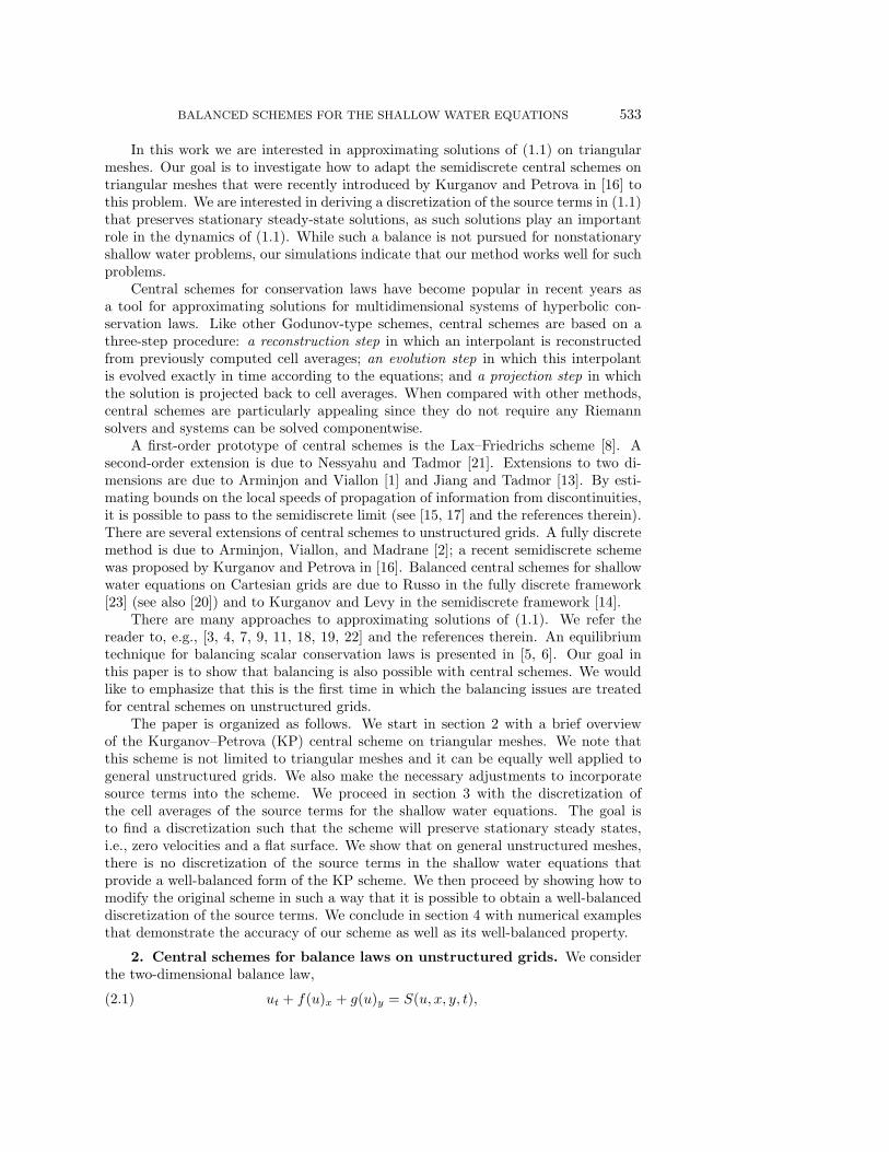
1. When the mesh is composed of triangles with one side that is parallel to thex-axis (see Figure 3.1), each cell has only two edges that contribute to the flux in thex-direction. In this case the system (3.9) can be solved. This result will enable usto introduce in section 3.2 a modification of the scheme (2.8) that can be balancedon general meshes. Due to symmetry considerations, such a mesh will not satisfythe balance conditions in the y-direction (that come from the third equation in (1.1))unless all triangles are right triangles that are aligned with both coordinate axes.


x

y

Fig. 3.1. An admissible triangular mesh.

2. The scheme can be balanced in both directions in the very special case ofCartesian grids. This corresponds to the case previously solved in [14]. The results of[14] when viewed from the point of view of the system (3.9) amount to the equality

B1(B1 − 2w) −B2(B2 − 2w) = (2w −B1 −B2)(B2 −B1).

Remark. If we assume a more general discretization of the cell average of (3.1) ofthe form

Sj = −N∑

k=1

gk(w −Bk)

N∑k′=1

akk′Bk′ ,(3.11)

then the system (3.9) is replaced by (denoting mk = mk/(2|Tj |))⎧⎪⎪⎪⎪⎨⎪⎪⎪⎪⎩

−2mk =∑N

k′=1 gk′ak′k, k = 1, . . . , N,

mk = −gkakk, k = 1, . . . , N,

gkakk′ = −gk′ak′k, k �= k′, k, k′ = 1, . . . , N.

(3.12)

The system (3.12) can be solved in the general case (unlike the system (3.9)). Forexample, in the case of a triangular grid (N = 3) one possible solution (assumingm1 �= 0 and m3 + 2m2 �= 0) is

g =

⎛⎜⎜⎝

−m1

m2 + m3

2

m3

2

⎞⎟⎟⎠, a =

⎛⎜⎜⎝

1 m3+2m2

2m1

m3

2m1

1 − 2m2

2m2+m3− m3

2m2+m3

1 1 −2

⎞⎟⎟⎠.(3.13)

If m1 = 0, the expression (3.13) can be replaced, e.g., by

g =

⎛⎜⎜⎝

0

m2 + m3

2

m3

2

⎞⎟⎟⎠, a =

⎛⎜⎜⎝

0 m3+2m2

m31

1 − 2m2

2m2+m3− m3

2m2+m3

1 1 −2

⎞⎟⎟⎠.(3.14)

If m3 + 2m2 = 0, a permutation of the numbering of the sides of the triangle willprovide a solution. Other solutions of (3.12) exist.

While formally being able to balance the scheme with the expressions (3.13) and(3.14), it remains unclear in what sense

∑k′ akk′Bk′ approximates the derivative Bx.

In other words, it is not obvious that the consistency of this discretization can beestablished. We therefore consider this approach unsatisfactory.


V1

V3

V2

V1

V2

V3

E2

E3

E1

E2

E3

E1

Fig. 3.2. The two types of triangles. Left: type 1. Right: type 2.

3.2. A new well-balanced scheme. The analysis in section 3.1 tells us thatbalancing the x-derivative flux term requires cells that have only 2 edges which havenormals with nonzero x-components (see Figure 3.1). This can be accomplished bysplitting our cells into subcells and solving the equation on these subcells. Similarly,the y-derivative flux term can be balanced by a different splitting of the cells. Wenow derive a new method based on this observation.

We focus on conformal triangular grids. Our ideas can be easily extended toother conformal unstructured meshes. In order to create a balanced scheme for (1.1),we propose to decompose every triangle Tj into several triangles as explained below.This requires a different decomposition for the two flux components. For the firstcomponent, f , we decompose Tj into two triangles, each of which has an edge parallelto the x-axis. For the second component of the flux we split Tj into two other triangles,each of which has an edge parallel to the y-axis.

We denote the vertices of Tj as Vjk, k = 1, 2, 3, and define the edges of Tj asEj1 = Vj2 −Vj1, Ej2 = Vj3 −Vj2, and Ej3 = Vj1 −Vj3. The midpoint of the kth edgeof Tj is Mjk. I (a, b) denotes the closed interval with endpoints a and b. We also useVjk,x (or Vjk,y) to denote the x (or y) component of Vjk. To simplify the treatment,we classify the triangles into two categories as portrayed in Figure 3.2.

(i) Type 1: one vertex Vj1 bisects the opposite edge in the y direction: they-component Vj1,y ∈ I (Vj2,y, Vj3,y) and a different vertex Vj2 bisects the oppositeedge in the x-direction: Vj2,x ∈ I (Vj1,x, Vj3,x). (See Figure 3.2 (left).)

(ii) Type 2: the same vertex Vj1 bisects the opposite edge in both the x and ydirections: Vj1,y ∈ I (Vj2,y, Vj3,y) and Vj1,x ∈ I (Vj2,x, Vj3,x). (See Figure 3.2 (right).)

Note that these definitions specify our vertex numbering convention. The decom-position for the g-flux will depend on the type of triangle.

3.2.1. The decomposition in the x-direction. For the flux in the x-direction,we decompose Tj into two triangles T x,1

j and T x,2j (see Figure 3.3). Define V x,1

j3

to be the intersection of edge Ej2 with the line y = Vj1,y. The vertices of T x,1j

are V x,1j1 := Vj1, V x,1

j2 := Vj2, and V x,1j3 . The vertices of T x,2

j are V x,2j1 := V x,1

j3 ,

V x,2j2 := Vj3, and V x,2

j3 := Vj1. For both triangles T x,ij , the lengths of the sides

are hx,ijk , the corresponding midpoints are Mx,i

jk , the interior and exterior speeds of

propagation are ain,out,x,ijk , and the normals are nx,i

jk = (nx,ijk,x, n

x,ijk,y). These definitions

imply Mx,1j1 = Mj1, M

x,2j2 = Mj3, h

x,1j1 = hj1, h

x,2j2 = hj3, h

x,1j2 + hx,2

j1 = hj2, nx,1j1 =


V1

V3

V2

Tx,1

Tx.2

M1 P

1

M3

P2

V3

x,1

Fig. 3.3. The triangle decomposition for the f-flux.

nj1,x, nx,1j2 = nx,2

j1 = nj2,x, nx,2j2 = nj3,x, and nx,1

j3,x = nx,2j3,x = 0. For the velocities

we have ain,out,x,1j1 = ain,out

j1 , ain,out,x,1j2 = ain,out

j2 , ain,out,x,2j1 = ain,out

j2 , and ain,out,x,2j2 =

ain,out

j3 . The velocity ain,out,x,ij3 does not play any role in the following computation since

nx,1j3,x = nx,2

j3,x = 0. Finally, the external reconstructions are denoted as ux,1j1 = uj1,

ux,1j2 = ux,2

j1 = uj2, and ux,2j2 = uj3.

On each triangle T x,ij we denote the cell average of the component of the flux in

the x-direction by Φij . It is given by

Φij = − 1

|T x,ij |

2∑k=1

hx,ijk n

x,ijk,x

ain,x,ijk + aout,x,i

jk

[ain,x,ijk f

(ux,ijk

(Mx,i

jk

))+ aout,x,i

jk f(uj

(Mx,i

jk

))]

for i = 1, 2. The cell average of the x-component of the flux over the entire cell Tj istaken to be the weighted average

Φj :=

∣∣∣T x,1j

∣∣∣|Tj |

Φ1j +

∣∣∣T x,2j

∣∣∣|Tj |

Φ2j .

Since∑3

k=1 hjknjk = 0 we have hx,1j1 nx,1

j1,x = −hx,1j2 nx,1

j2,x and hx,2j2 nx,2

j2,x = −hx,2j1 nx,2

j1,x.Hence, Φj can be rewritten as

Φj = −hj1nj1,x

|Tj |

[ainj1f

outj1 + aout

j1 finj1

ainj1 + aout

j1

−ainj2f (uj2 (Pj1)) + aout

j2 f (uj (Pj1))

ainj2 + aout

j2

](3.15)

−hj3nj3,x

|Tj |

[ainj3f

outj3 + aout

j3 finj3

ainj3 + aout

j3


j2 f (uj (Pj2))

ainj2 + aout

j2

],

where Pj1 := Mx,1j2 and Pj2 := Mx,2

j1 .Remark. We would like to note that the flux term (3.15) can be derived directly

from (2.6) by changing the quadrature points on Ej2 to P1 and P2.


V1

V2

V3

V1

V3

V2

Ty,1

Ty.2

M1

P3

M2

P4

V1

y,1V

1y,1

Ty,1

Ty.2

M1

M3

P4

P3

Fig. 3.4. The triangle decomposition for the g-flux. Left: type 1. Right: type 2.

3.2.2. The decomposition in the y-direction.Type 1 triangles. We decompose Tj into two triangles T y,1

j and T y,2j (see

Figure 3.4 (left)). The intersection of the edge Ej3 with the line x = Vj2,x is denoted

by V y,1j1 . The vertices of T y,1

j are V y,1j1 , V y,1

j2 := Vj1, and V y,1j3 := Vj2. The vertices

of T y,2j are V y,2

j1 := Vj2, Vy,2j2 := Vj3, and V y,2

j3 := V y,1j1 . As before, we have My,1

j2 =

Mj1, My,2j1 = Mj2, hy,1

j2 = hj1, hy,2j1 = hj2, hy,1

j1 + hy,2j2 = hj3. The normals are

ny,1j2 = nj1, n

y,1j1 = ny,2

j2 = nj3, ny,2j1 = nj2, n

y,1j3,y = ny,2

j3,y = 0 and the velocities are

ain,out,y,1j1 = ain,out

j3 , ain,out,y,1j2 = ain,out



j3 . The velocity

ain,out,y,ij3 does not appear in the result because ny,1

j3,y = ny,2j3,y = 0. Finally, the external

reconstructions are uy,1j1 = uj3, u

y,1j2 = uj1, u

y,2j1 = uj2, and uy,2

j2 = uj3.We denote the cell averages of the component of the flux in the y-direction on

each triangle T y,ij by Γi

j . It is given by

Γij := − 1

|T y,ij |

2∑k=1

hy,ijk n

y,ijk,y

ain,y,ijk + aout,y,i

jk

[ain,y,ijk g

(uy,ijk

(My,i

jk

))+ aout,y,i

jk g(uj

(My,i

jk

))]

for i = 1, 2. The cell average of the y-component of the flux over the entire cell Tj isthen given by the weighted average

Γj :=

∣∣∣T y,1j

∣∣∣|Tj |

Γ1j +

∣∣∣T y,2j

∣∣∣|Tj |

Γ2j .

Clearly hy,1j2 ny,1

j2,y = −hy,1j1 ny,1

j1,y and hy,2j1 ny,2

j1,y = −hy,2j2 ny,2

j2,y. Therefore Γj can berewritten as

Γj = −hj1nj1,y

|Tj |

[ainj1g

outj1 + aout

j1 ginj1

ainj1 + aout

j1

−ainj3g (uj3 (Pj3)) + aout

j3 g (uj (Pj3))

ainj3 + aout

j3

](3.16)

−hj2nj2,y

|Tj |

[ainj2g

outj2 + aout

j2 ginj2

ainj2 + aout

j2


j3 g (uj (Pj4))

ainj3 + aout

j3

],


where Pj3 := My,1j1 and Pj4 := My,2

j2 .

Type 2 triangles. This case corresponds to Figure 3.4 (right). Analogouscomputations to those for type 1 triangles provide the cell average of the y-componentof the flux over the cell Tj , which this time is given by

Γj = −hj1nj1,y

|Tj |

[ainj1g

outj1 + aout

j1 ginj1

ainj1 + aout

j1


j2 g (uj (Pj3))

ainj2 + aout

j2

](3.17)

−hj3nj3,y

|Tj |

[ainj3g

outj3 + aout

j3 ginj3

ainj3 + aout

j3


j2 g (uj (Pj4))

ainj2 + aout

j2

],

where Pj3 and Pj4 are given in Figure 3.4 (right).

3.2.3. The new method (for conservation laws). We would now like tocombine all the different ingredients that we developed in the previous section into onescheme. The scheme that we write here is still a scheme for approximating solutions ofthe conservation law (2.2) without the source term. Based on our preliminary analysisof section 3.1 we know that we will be able to find an admissible discretization of thesource terms that will result with a well-balanced scheme. We will treat the sourceterms in the next section.

We write two versions of the scheme based on the type of triangle. For type 1triangles, the discretization of the component of the flux in the x-direction, Φj is givenby (3.15) while the discretization of the component of the flux in the y-direction, Γj ,is given by (3.16). In this case the scheme takes the form

duj

dt= −hj1nj1,x

|Tj |

[ainj1f

outj1 + aout

j1 finj1

ainj1 + aout

j1


j2 f (uj (Pj1))

ainj2 + aout

j2

]

−hj3nj3,x

|Tj |

[ainj3f

outj3 + aout

j3 finj3

ainj3 + aout

j3


j2 f (uj (Pj2))

ainj2 + aout

j2

]

−hj1nj1,y

|Tj |

[ainj1g

outj1 + aout

j1 ginj1

ainj1 + aout

j1


j3 g (uj (Pj3))

ainj3 + aout

j3

](3.18)

−hj2nj2,y

|Tj |

[ainj2g

outj2 + aout

j2 ginj2

ainj2 + aout

j2

−ainj3g (uj3 (Pj4)) + ain

j3g (uj (Pj4))

ainj3 + aout

j3

]

+1

|Tj |

3∑k=1

hjk

ain

jkaout

jk

ain

jk + aout

jk

[uout

jk − uin

jk

].

Here P1 = V2 − 12E1,y

E2,yE2, P2 = V3 + 1

2E3,y

E2,yE2, P3 = V1 + 1

2E1,x

E3,xE3, and P4 = V3 −

12E2,x

E3,xE3.

For type 2 triangles we replace the discretization of Γj by the one given in (3.17)


ending with

duj

dt= −hj1nj1,x

|Tj |

[ainj1f

outj1 + aout

j1 finj1

ainj1 + aout

j1


j2 f (uj (Pj1))

ainj2 + aout

j2

]

−hj3nj3,x

|Tj |

[ainj3f

outj3 + aout

j3 finj3

ainj3 + aout

j3


j2 f (uj (Pj2))

ainj2 + aout

j2

]

−hj1nj1,y

|Tj |

[ainj1g

outj1 + aout

j1 ginj1

ainj1 + aout

j1


j2 g (uj (Pj3))

ainj2 + aout

j2

](3.19)

−hj3nj3,y

|Tj |

[ainj2g

outj3 + aout

j2 ginj3

ainj3 + aout

j3

−ainj2g (uj2 (Pj4)) + ain

j2g (uj (Pj4))

ainj2 + aout

j2

]

+1

|Tj |

3∑k=1

hjk

ain

jkaout

jk

ain

jk + aout

jk

[uout

jk − uin

jk

].

In this case P1 = V2 − 12E1,y

E2,yE2, P2 = V3 + 1

2E3,y

E2,yE2, P3 = V2 − 1

2E1,x

E2,xE2, and

P4 = V3 + 12E3,x

E2,xE2.

Remarks.

1. For a general triangulation our method will not be conservative because thefluxes from adjacent triangles will not in general be evaluated at the same point onthe edge. Our tests with irregular triangulations in section 4 show, however, that thisfailure of conservation does not lead to serious problems.

2. A simple case of interest is that of coordinate-aligned right triangles. Suchtriangles can be considered to be of type 1 with nj2,y = nj3,x = 0 and Pj1 = Mj2

and Pj3 = Mj3, which means that the method becomes (taking into account that∑3k=1 hjknjk = 0)

duj

dt= − 1

|Tj |

[ainj1f

outj1 + aout

j1 finj1

ainj1 + aout

j1

hj1nj1,x +ainj2f

outj2 + aout

j2 finj1

ainj2 + aout

j2

hj2nj2,x

]

− 1

|Tj |

[ainj1g

outj1 + aout

j1 ginj1

ainj1 + aout

j1

hj1nj1,y +ainj3g

outj3 + aout

j3 ginj1

ainj3 + aout

j3

hj3nj3,y

](3.20)

+1

|Tj |

3∑k=1

hjk

ain

jkaout

jk

ain

jk + aout

jk

[uout

jk − uin

jk

].

As expected, in this case the method (3.20) coincides with the KP method (2.7).

3.2.4. Adding the source term. We return to the shallow water equations(1.1). Our goal is now to find an admissible discretization of the cell average of thesource terms that will preserve stationary steady states. Such a term will be addedto the RHS of (3.18) or (3.19) depending on the type of the triangle. In the followingwe assume type 1 triangles. Similar analysis holds for type 2 triangles. We also notethat the first equation in the system (1.1) is homogeneous. This means that we onlyhave to consider the remaining two equations when dealing with the source terms.We recall from section 3.1 that in stationary steady states all the velocities are equal,ain

jk = aout

jk = ajk. Our new method (3.18) for the last two equations of (1.1) then


becomes

(3.21)

0 = −hj1nj1,x

2 |Tj |

[((w (Mj1) −B (Mj1))

2

0

)−(

(w (Pj1) −B (Pj1))2

0

)]

−hj3nj3,x

2 |Tj |

[((w (Mj3) −B (Mj3))

2

0

)−(

(w (Pj2) −B (Pj2))2

0

)]

−hj1nj1,y

2 |Tj |

[(0

(w (Mj1) −B (Mj1))2

)−(

0

(w (Pj3) −B (Pj3))2

)]

−hj2nj2,y

2 |Tj |

[(0

(w (Mj2) −B (Mj2))2

)−(

0

(w (Pj4) −B (Pj4))2

)]+

(S1j

S2j

).

The last term in (3.21) represents the average of the source, i.e., S1j = avg(−(w −

B)Bx) and S2j = avg(−(w −B)By), where both averages are taken over Tj .

We use (3.21) to determine the admissible discretizations of the cell averages ofthe source terms. For constant w the source terms (given by (3.21)) can be rewrittenas

S1j = −hj1nj1,x

2|Tj |[wMj1

−BMj1+ wPj1

−BPj1][BMj1

−BPj1]

−hj3nj3,x

2|Tj |[wMj3 −BMj3 + wPj2 −BPj2 ][BMj3 −BPj2 ],(3.22)

S2j = −hj1nj1,y

2|Tj |[wMj1 −BMj1

+ wPj3 −BPj3 ][BMj1 −BPj3]

−hj2nj2,y

2|Tj |[wMj2 −BMj2

+ wPj4 −BPj4 ][BMj2 −BPj4 ].

Here, we use the notation wM1 := w (Mj1), etc. We take the expressions in (3.22) asthe discretization of the source even when w is not constant. Similar expressions canbe easily written for type 2 triangles.

Lemma 3.1. The source discretizations Sij given by (3.22) are consistent approx-

imations of the source terms in (1.1) and lead to detailed balance in the stationarysteady-state case (3.21).

Before proving Lemma 3.1 we consider the following geometrical lemma.Lemma 3.2. With M and P defined as in section 3.2.1 (suppressing j),

M1,x − P1,x = − |T |h2n2,x

, M3,x − P2,x = − |T |h2n2,x

.

Proof. M1 = 12 (V1 + V2), and for some s, P1 = V2 + s (V3 − V2). We require that

P1,y = M1,y, which implies that

s =1

2

V1,y − V2,y

V3,y − V2,y.

Therefore

M1,x − P1,x =1

2(V1,x + V2,x) − V2,x − 1

2

V1,y − V2,y

V3,y − V2,y(V3,x − V2,x) = −1

2

E1 × E2

E2,y.


When the orientation of the vertices of Tj is clockwise, E1 × E2 = −2 |T | and n2 =1h2

(−E2,y, E2,x), while when the orientation is counterclockwise, E1 ×E2 = 2 |T | and

n2 = 1h2

(E2,y,−E2,x), so

M1,x − P1,x = − |T |h2n2,x

.

Similar arguments hold for M3,x − P2,x.Proof of Lemma 3.1. We show that S1

j ≈ avg(−(w − B)Bx). To simplify thenotations we suppress the index j. From Lemma 3.2 we know that M1,x − P1,x =

− |T |h2n2,x

. Since M1,y = P1,y we haveBM1

−BP1

M1,x−P1,x= Bx +O(|M1 − P1|2) at the midpoint

between M1 and P1. Hence the first part of S1j in (3.22) becomes

h1n1,x

2h2n2,x(wM1 −BM1 + wP1 −BP1)

BM1 −BP1

M1,x − P1,x

≈ h1n1,x

2h2n2,x(wM1

−BM1+ wP1

−BP1)Bx.

Applying a similar argument to the second term of S1j in (3.22) gives

S1j ≈ 1

2

(h1n1,x

h2n2,x(wM1

−BM1+ wP1

−BP1)(3.23)

+h3n3,x

h2n2,x(wM3

−BM3+ wP2

−BP2)

)Bx.

Clearly, the coefficient of Bx in (3.23) is a discretization of a weighted average of−(w −B). For example, when w −B is constant we have

S1j ≈ h1n1,x + h3n3,x

h2n2,x(w −B)Bx = − (w −B)Bx.

Similar arguments hold for S2j .

Remark. If we consider a Cartesian mesh split into triangles along a diagonal, itis easy to see that our method reduces to the method in [14].

4. Numerical examples. The scheme developed in section 3.2 did not assumeany particular reconstruction. There are several different second-order reconstructionson triangular meshes that are being used in the literature (see [16] and the referencestherein). We briefly describe the one we used in our simulations.

The starting point is the limited least-squares estimate of the gradients as donein [2]. The first step is to compute a least-squares estimate of the gradient of a fieldf on the triangle Tj , ∇jf . We then limit the gradient Djf component by componentas

Djf = MM(∇jf, ∇j1f, ∇j2f, ∇j3f

),

where ∇jkf is the least-squares gradient estimate on Tjk and MM stands for the usualMinMod limiter

MM (x1, x2, . . . ) :=

⎧⎨⎩

minj {xj} if xj > 0 ∀j,maxj {xj} if xj < 0 ∀j,0 otherwise.


Fig. 4.1. The two types of triangle meshes. Left: Uniform triangulation. Right: Perturbed(nonuniform) triangulation.

We use the gradients Dj to construct a piecewise linear reconstruction for the pointvalues of each triangle edge Ejk as

uj(�x) = uj + MM (Dju · (�x− �xj) ,Djku · (�x− �xj)).

Here Djku is the limited gradient estimate on Tjk, �xj is the center of Tj , and �x ∈ Ejk.We find that this double use of the MinMod limiter minimizes spurious oscillationswhile preserving the second-order accuracy of the reconstruction.

We use an adaptive time step given by

Δt = 0.9 minj

rj

|λjN |

,

where rj is the radius of Tj and |λjN | is the norm of the largest eigenvalues of the

Jacobian of the flux on Tj .We use two types of meshes in most of our simulations. The first is a uniform

triangulation of a Cartesian mesh with N ×N nodes and constant spacings Δx andΔy, which divides each Cartesian cell into four triangles. To test our method onmore general meshes, our second type of mesh is generated from a uniform triangularmesh with a perturbation of the coordinates of the interior vertices. Examples ofboth meshes are shown in Figure 4.1. The only exception is Example 6, which uses auniform triangulation of a warped Cartesian mesh.

Example 1: Accuracy tests for a two-dimensional Burgers equation.We test the accuracy of our method (3.18)–(3.19) on nonlinear problems by applyingit to the two-dimensional Burgers equation⎧⎨

⎩ut + 1

2

(u2

)x

+ 12

(u2

)y

= 0, [−2π, 2π]2,

u (x, y, t = 0) = sin(x+y

2

),

(4.1)

with periodic boundary conditions. The relative L1-error (i.e., the L1-error divided bythe L1-norm of the exact solution) of our method at T = 0.5 is shown in Table 4.1 foruniform and perturbed triangulations. The computed cell averages after singularityformation at T = 1.5 are shown in Figure 4.2. Note the sharp shocks that are capturedby our method.


Table 4.1

L1-error and convergence rates for Burgers equation (4.1) at T = 0.5 on a uniform and aperturbed triangulation of an N ×N Cartesian mesh.

Uniform triangulation Perturbed triangulation

N Relative L1-error L1-order Relative L1-error L1-order

10 0.064 — 0.064 —20 0.014 2.20 0.014 2.2040 4.68 × 10−3 1.58 4.65 × 10−3 1.5980 1.37 × 10−3 1.77 1.36 × 10−3 1.77

–10

–5

0

5

10 –10

–5

0

5

10–1

–0.5

0

0.5

1

x

y

u

–10 0 –10 0 10

–1

–0.8

–0.6

–0.4

–0.2

0

0.2

0.4

0.6

0.8

1Side view

u

x y

Fig. 4.2. Burgers equation at T = 1.5 on a uniform triangulation of a 20× 20 Cartesian mesh.Left: oblique view. Right: side view.

Example 2: The Sod problem. To test our method (3.18)–(3.19) on a systemof equations we apply it to the Sod problem for the Euler equations⎛

⎜⎜⎝ρρuρvE

⎞⎟⎟⎠

t

+

⎛⎜⎜⎝

ρuρu2 + pρuv

u (E + p)

⎞⎟⎟⎠

x

+

⎛⎜⎜⎝

ρvρuv

ρv2 + pv (E + p)

⎞⎟⎟⎠

y

= 0.(4.2)

Here ρ is the density, (u, v) is the velocity, and E is the energy. The equation of statefor the pressure is p = (γ − 1)

[E − ρ

2

(u2 + v2

)]. We set γ = 1.4 and take the initial

conditions (constant in the y-direction)

(p, ρ, u, v) =

{(1.0, 1.0, 0.0, 0.0) , x < 0.5,(0.1, 0.125, 0.0, 0.0) , x > 0.5.

(4.3)

Figure 4.3 shows the computed cell averages at T = 0.16 using our method fromsection 3.2 projected onto the y = 0 plane. A reference one-dimensional solution is alsoshown. The two-dimensional problem is run on both a uniform triangulation basedon a 300× 30 Cartesian mesh on the domain [0, 1]× [0, 0.1] as well as a perturbationof that mesh. The one-dimensional reference solution is computed using the second-order central method of [15] with 3000 points in the domain [0, 1]. As expected, thequality of the solution slightly degrades on the nonuniform mesh.

Example 3: A balance test. In this example we demonstrate the well-balancedproperty of our scheme (3.18)–(3.19) with the source discretization (3.22).


0 0.5 10

0.2

0.4

0.6

0.8

1

pres

sure

x0 0.5 1

0

0.2

0.4

0.6

0.8

1

u

x

0 0.5 10

0.2

0.4

0.6

0.8

1

pres

sure

x0 0.5 1

0

0.2

0.4

0.6

0.8

1

u

x

Fig. 4.3. The pressure (left) and u-velocity (right) fields of the Sod problem at T = 0.16 on auniform triangulation (top) and a perturbed triangulation (bottom). The circles show an orthogonalprojection onto the y = 0 plane of the solution of the two-dimensional problem on a triangular mesh.The line shows a one-dimensional reference solution computed with the second-order central-upwindmethod of [15].

As a simple test of balance, we consider the shallow water problem with initialconditions that represent a stationary steady state. We choose w (x, y, t = 0) = 2,u (x, y, t = 0) = v (x, y, t = 0) = 0, and a bottom topography given by B (x, y) =sin(2πx) + cos(2πy) on the domain [0, 1]2. We assume periodic boundary conditions.This initial value problem has the trivial stationary steady-state solution w (x, y, t) =2, u (x, y, t) = v (x, y, t) = 0 for all t.

The relative L1-errors at T = 1 on both uniform and perturbed triangulationsbased on a 10 × 10 Cartesian mesh are given in Table 4.2. This table also showsthe result found using the KP method [16] with the same source discretization (3.22)which is not balanced for this scheme. We see that our method balances to machineaccuracy.

Example 4: Propagating waves with a bottom topography. We apply ourmethod to a test problem from [18] of a small perturbation of a steady-state problemon the domain [0, 2]× [0, 1] with periodic boundary conditions in the y-direction. Thebottom topography is the elliptical Gaussian mound given by

B (x, y) = 0.8 exp(−5 (x− 0.9)

2 − 50 (y − 0.5)2),


Table 4.2

The relative L1-error in the balance for (3.18), (3.19), (3.22) and for the KP scheme with thesource discretization (3.22).

Method Uniform triangulation Perturbed triangulation

(3.18)–(3.19)–(3.22) 3.5 × 10−17 6.9 × 10−19

[16] + (3.22) 3.0 × 10−3 3.5 × 10−3

0 0.5 1 1.5 20

0.5

1T=0.6

0 0.5 1 1.5 20

0.5

1T=0.9

0 0.5 1 1.5 20

0.5

1T=1.2

0 0.5 1 1.5 20

0.5

1T=1.5

0 0.5 1 1.5 20

0.5

1T=1.8

0 0.5 1 1.5 20

0.5

1T=0.6

0 0.5 1 1.5 20

0.5

1T=0.9

0 0.5 1 1.5 20

0.5

1T=1.2

0 0.5 1 1.5 20

0.5

1T=1.5

0 0.5 1 1.5 20

0.5

1T=1.8

Fig. 4.4. Wave propagation over an elliptical hump at various times. Left: uniform triangula-tion based on a 200 × 100 mesh. Right: uniform triangulation based on a 400 × 200 mesh.


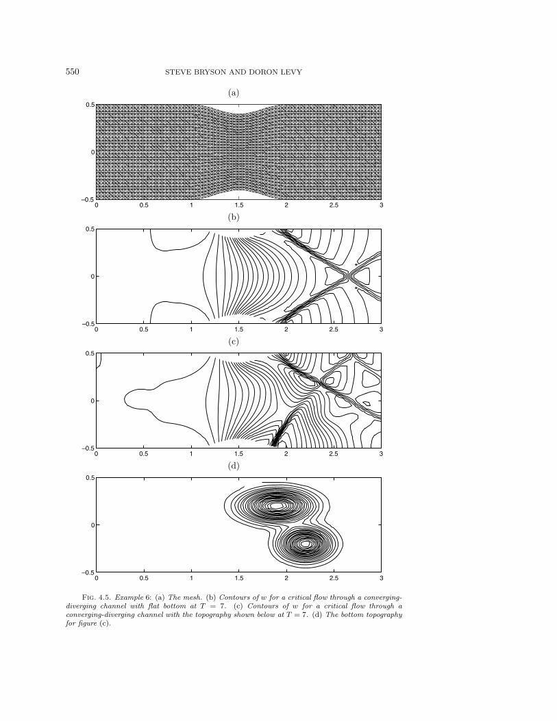
(a)

0 0.5 1 1.5 2 2.5 3–0.5

0

0.5

(b)

0 0.5 1 1.5 2 2.5 3–0.5

0

0.5

(c)

0 0.5 1 1.5 2 2.5 3–0.5

0

0.5

(d)

0 0.5 1 1.5 2 2.5 3–0.5

0

0.5

Fig. 4.5. Example 6: (a) The mesh. (b) Contours of w for a critical flow through a converging-diverging channel with flat bottom at T = 7. (c) Contours of w for a critical flow through aconverging-diverging channel with the topography shown below at T = 7. (d) The bottom topographyfor figure (c).


and the initial conditions are

(w, u, v) =

{(1.01, 0.0, 0.0) if 0.05 < x < 0.15,(1.0, 0.0, 0.0) otherwise.

Figure 4.4 shows the result of our method at various times on a uniform triangulationof both a 200×100 and 400×200 Cartesian mesh. These results are in good agreementwith other methods on Cartesian grids (see [14, 18]).

Example 5: Converging-diverging channel with bottom topography.Our final example is that of a converging-diverging channel with critical flow adaptedfrom [12]. The channel is defined on the domain [0, 3] × [−0.5, 0.5] with a half-cosineconstriction centered at x = 1.5. The mesh for this example is shown in Figure 4.5(a).It is a nonuniform triangulation obtained by warping a uniform triangulation of aCartesian mesh under the mapping (x, y) →

(x,

(1 − 0.2 cos2 (π (x− 1.5))

)y)

when|x− 1.5| < 0.5. The initial data is w = 1, u = v = 0. The y-boundaries are reflecting.The left x-boundary is an inflow boundary with u = 5.0 and the right x-boundaryis a zeroth-order outflow boundary. We run the simulations on a 90 × 30 mesh untilT = 7 after the steady state is achieved. We would like to emphasize that this is nota stationary steady state.

We first present this example with a flat bottom, with contours of w shown inFigure 4.5(b). Figure 4.5(c) shows the same channel at the same time with bottomtopography

B (x, y) = 0.8(exp

(−10 (x− 1.9)

2 − 50 (y − 0.2)2)

+ exp(−20 (x− 2.2)

2 − 50 (y + 0.2)2))

.

This topography is shown in Figure 4.5(d) and represents two elliptical Gaussianmounds just downflow from the constriction.

We choose the initial and boundary conditions such that stationary shocks aregenerated. The symmetry of the flat-bottom case (Figure 4.5(b)) is broken by thenonsymmetric bottom (Figures 4.5(c)–(d)). These results are in qualitative agreementwith those that are shown in [12]. We note that the simulations in [12] correspondonly to the flat bottom case.

5. Conclusion. In this paper we presented a well-balanced semidiscrete centralscheme on triangular meshes for shallow water equations with bottom topography.This scheme is derived by changing the quadrature rules for the flux integrals thatwere proposed in [16]. A careful discretization of the source term then allows us topreserve stationary steady states.

The numerical flux is complemented by a new second-order reconstruction ontriangular meshes. The accuracy and well-balanced properties of the scheme aredemonstrated in a variety of numerical simulations.

Several generalizations of this scheme are left for future research. This includesdry beds and dissipative systems.

Acknowledgments. We would like to thank Jonathan Goodman and BenoitPerthame for helpful discussions.


REFERENCES

[1] P. Arminjon and M.-C. Viallon, Generalisation du schema de Nessyahu-Tadmor pour uneequation hyperbolique a deux dimensions d’espace, C. R. Acad. Sci. Paris Ser. I Math., 320(1995), pp. 85–88.

[2] P. Arminjon, M.-C. Viallon, and A. Madrane, A finite volume extension of the Lax-Friedrichs and Nessyahu-Tadmor schemes for conservation laws on unstructured grids,Int. J. Comput. Fluid Dyn., 9 (1997), pp. 1–22.

[3] E. Audusse and M.-O. Bristeau, Transport of pollutant in shallow water: A two time stepskinetic method, M2AN Math. Model. Numer. Anal., 37 (2003), pp. 389–416.

[4] E. Audusse, M.-O. Bristeau, and B. Perthame, Kinetic Schemes for Saint-Venant Equa-tions with Source Terms on Unstructured Grids, INRIA report RR-3989, 2000.

[5] R. Botchorishvili, B. Perthame, and A. Vasseur, Equilibrium schemes for scalar conser-vation laws with stiff sources, Math. Comp., 72 (2003), pp. 131–157.

[6] R. Botchorishvili and O. Pironneau, Finite volume schemes with equilibrium-type dis-cretization of source terms for scalar conservation laws, J. Comput. Phys., 187 (2003),pp. 391–427.

[7] A. I. Delis and Th. Katsaounis, Relaxation schemes for the shallow water equations, Internat.J. Numer. Methods Fluids, 41 (2003), pp. 695–719.

[8] K. O. Friedrichs and P. D. Lax, Systems of conservation equations with a convex extension,Proc. Natl. Acad. Sci. USA, 68 (1971), pp. 1686–1688.

[9] T. Gallouet, J.-M. Herard, and N. Seguin, Some approximate Godunov schemes to computeshallow-water equations with topography, Comput. & Fluids., 32 (2003), pp. 479–513.

[10] J. F. Gerbeau and B. Perthame, Derivation of viscous Saint-Venant system for laminarshallow water; numerical validation, Discrete Contin. Dyn. Syst. Ser. B, 1 (2001), pp. 89–102.

[11] L. Gosse, A well-balanced scheme using non-conservative products designed for hyperbolicsystems of conservation laws with source terms, Math. Models Methods Appl. Sci., 11(2001), pp. 339–365.

[12] M. E. Hubbard, On the accuracy of one-dimensional models of steady converging/divergingopen channel flows, Internat. J. Numer. Methods Fluids, 35 (2001), pp. 785–808.

[13] G.-S. Jiang and E. Tadmor, Nonoscillatory central schemes for multidimensional hyperbolicconservation laws, SIAM J. Sci. Comput., 19 (1998), pp. 1892–1917.

[14] A. Kurganov and D. Levy, Central-upwind schemes for the Saint-Venant system, M2ANMath. Model. Numer. Anal., 36 (2002), pp. 397–425.

[15] A. Kurganov, S. Noelle, and G. Petrova, Semidiscrete central-upwind schemes for hyper-bolic conservation laws and Hamilton–Jacobi equations, SIAM J. Sci. Comput., 23 (2001),pp. 707–740.

[16] A. Kurganov and G. Petrova, Central-upwind schemes on triangular grids for hyperbolicsystems of conservation laws, Numer. Methods Partial Differential Equations, 21 (2005),pp. 536–552.

[17] A. Kurganov and E. Tadmor, New high-resolution central schemes for nonlinear conservationlaws and convection-diffusion equations, J. Comput. Phys., 160 (2000), pp. 214–282.

[18] R. J. LeVeque, Balancing source terms and flux gradients in high-resolution Godunov meth-ods: The quasi-steady wave-propagation algorithm, J. Comput. Phys., 146 (1998), pp. 346–365.

[19] R. J. LeVeque and D. S. Bale, Wave propagation methods for conservation laws with sourceterms, in Hyperbolic Problems: Theory, Numerics, Applications, Vol. II (Zurich, 1998),Internat. Ser. Numer. Math. 130, Birkhauser, Basel, 1999, pp. 609–618.

[20] S. F. Liotta, V. Romano, and G. Russo, Central schemes for systems of balance laws, inHyperbolic Problems: Theory, Numerics, Applications, Vol. II (Zurich, 1998), Internat.Ser. Numer. Math. 130, Birkhauser, Basel, 1999, pp. 651–660.

[21] H. Nessyahu and E. Tadmor, Non-oscillatory central differencing for hyperbolic conservationlaws, J. Comput. Phys., 87 (1990), pp. 408–463.

[22] B. Perthame and C. Simeoni, A kinetic scheme for the Saint-Venant system with a sourceterm, Calcolo, 38 (2001), pp. 201–231.

[23] G. Russo, Central schemes for balance laws, in Hyperbolic Problems: Theory, Numerics, Ap-plications, Vol. I, II (Magdeburg, 2000), Internat. Ser. Numer. Math. 140, 141, Birkhauser,Basel, 2001, pp. 821–829.

[24] A. J. C. de Saint-Venant, Theorie du mouvement non-permanent des eaux, avec applicationaux crues des riviere at a l’introduction des marees dans leur lit, C. R. Acad. Sci. Paris,73 (1871), pp. 147–154.

Date post:	14-Feb-2018
Category:	Documents
Upload:	lycong
View:	218 times
Download:	0 times

BALANCED CENTRAL SCHEMES FOR THE SHALLOW …dlevy/papers/water-sisc.pdf · Vol. 27, No. 2, pp....

Documents