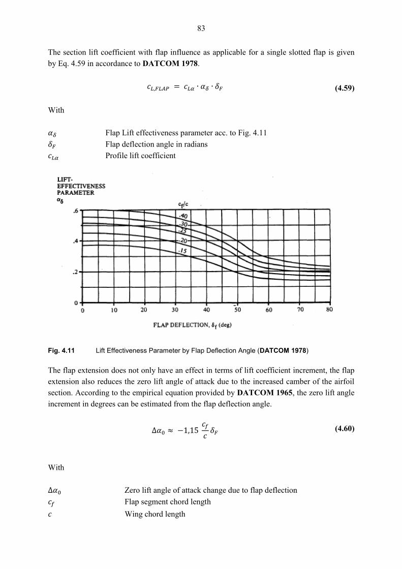
Page 1
Bachelor Thesis
Department Automotive and Aeronautical Engineering
Balanced Field Length Calculation for a Learjet 35A/36A with Under-Wing Stores on a Wet Runway
Florian Ehrig 31. August 2012
Page 2
2
Hochschule für Angewandte Wissenschaften Hamburg Fakultät Technik und Informatik Department Fahrzeugtechnik + Flugzeugbau Berliner Tor 9 20099 Hamburg
In Cooperation with: GFD Gesellschaft für Flugzieldarstellung mbH An EADS Subsidiary Flugplatz Hohn 24806 Hohn
Author: Florian Ehrig Date of Examination: 31.08.2012 1
st Examiner: Prof. Dr.-Ing. Dieter Scholz, MSME
2nd
Examiner: Prof. Dr.-Ing. Hartmut Zingel Industrial Supervising Tutor: Dipl.-Ing. Enrico Busse
Scholz
Notiz
Commercial use strictly prohibited. Your request may be directed to: Prof. Dr.-Ing. Dieter Scholz, MSME E-Mail see: http://www.ProfScholz.de Download this file from: http://Bibliothek.ProfScholz.de
Page 3
3
Abstract
The Learjet 35A/36A is a twin-engine business jet. In a special configuration, it can be fitted
with under-wing stores, a configuration for which no takeoff performance data on wet run-
ways is currently available. This report outlines the creation of a numerical takeoff perfor-
mance simulation for this specific aircraft on wet runways. The results shall be used to set up
takeoff performance charts that can be used in daily flight operations.
To obtain Balanced Field Lengths and Decision Speeds according to EASA CS-25 certifica-
tion specifications, the aircraft acceleration, takeoff and braking performance was determined.
A comprehensive aircraft parameter estimation has been performed, permitting to consider the
forces acting on the aircraft in various takeoff phases accurately in their dependency of time
and speed.
A focus of the parameter investigation was put on the precipitation drag acting on the aircraft
due to the wet runway conditions. A specific geometry-based investigation of the factors de-
termining the amount of spray drag acting on the Learjet 35A/36A airframe with under-wing
stores was performed. This permitted a conclusion on the additional drag due to water im-
pingement on the aircraft in the special takeoff configuration.
The results of the simulation were set in relation with the existing aircraft performance data
and a simplified calculation method. It was found that the simulation produces results of high
accuracy and the results show consistent behavior with a variation in input parameters.
Page 4
4
DEPARTMENT FAHRZEUGTECHNIK UND FLUGZEUGBAU
Balanced Field Length Calculation for a Learjet
35A/36A with Under-Wing Stores on a Wet Runway
Task for a Bachelor Thesis according to University Regulations
Background
Eleven aircraft of type Learjet 35A and Learjet 36A are operated by the company GFD Ge-
sellschaft für Flugzieldarstellung mbH based on the Military Airfield Hohn in the north of
Germany. The GFD-owned aircraft can be operated as Special Mission Aircraft with stores
mounted under each wing carrying external loads of up to 900 lbs (408 kg) on each side. Of
interest is the calculation of the Takeoff Field Length (TOFL) of the GFD Learjets when op-
erated with under-wing stores on a wet runway. The TOFL is the greater of the Balanced
Field Length (BFL) and 115% of the All-Engines-Operative Takeoff Distance. The BFL is
determined by the condition that the distance to continue a takeoff following a failure of an
engine at a critical engine failure speed is equal to the distance required to abort it. It repre-
sents the worst case scenario, since a failure at a lower speed requires less distance to abort,
whilst a failure at a higher speed requires less distance to continue the takeoff. V11 during
takeoff is the maximum speed at which the pilot is able to take the first action to stop the air-
plane (apply brakes) within the accelerate-stop distance and at the same time the minimum
speed at which the takeoff can be continued to achieve the required height above the takeoff
surface within the takeoff distance. The title of the project names specifically the BFL as it is
usually the distance that determines the TOFL for aircraft with two engines.
1 Critical Engine Failure Recognition Speed or Takeoff Decision Speed
Page 5
5
Task
Set up a calculation / simulation based on the integration of the differential equation describ-
ing the aircraft motion under BFL conditions to output the BFL and V1. The calculation
should be done for a set of specified input data. The simulation should be compared to per-
formance data from the Airplane Flight Manual (AFM).
Detailed tasks are:
Literature review and description of operational hazards during takeoff on wet and
contaminated runways.
Collection of all required geometrical and performance data of the Learjet 35A/36A.
Detailed review of certification rules related to takeoff performance calculations.
Derivation of equations required for the calculation / simulation of the BFL.
Literature review and extraction of key equations for the calculation of drag on a roll-
ing aircraft caused by a wet or contaminated runway (in contrast to a dry runway).
Investigation of further details for the performance calculation of the Learjet
35A/36A: Aircraft drag polar, drag due to spoilers, lift decrease due to spoilers, thrust
decay with speed and air density, idle thrust, brake coefficients, braking capabilities, ...
Set up, description, calibration and verification of the calculation / simulation.
Calculation of BFL and V1 for a set of specified input data.
Comparison of calculation results with simpler approaches (BFL from Raymer 1989;
other TOFL estimation methods).
The report should be written in English based on German standards on report writing.
Page 6
6
Declaration
I affirm that this report has been written entirely on my own, having used only the indicated
references and tools. Where citations have been taken from other work than the present report,
the source has been fully acknowledged and referenced.
Date Signature
Page 7
7
Acknowledgements
I would like to express my sincere appreciation to all supervisors that have been accompany-
ing me during the course of the project. Without the invaluable advice that only their experi-
ence and expertise could have provided, this work would not have been possible.
I am indebted to Prof. Dr.-Ing. Dieter Scholz, MSME, Dipl.-Ing. Enrico Busse and Dipl.-Ing.
Svend Engemann for having given me the opportunity to elaborate my bachelor thesis on this
exciting topic, and for their assistance and support provided in solving the challenges it in-
volved.
My special gratitude goes to Mr. Enrico Busse, who took a lot of time to provide excellent
advice, suggestions and help towards the creation of a sound report. His experience as certifi-
cation engineer and Learjet pilot that he shared with me on numerous occasions has contribut-
ed greatly to my formation in becoming an aeronautical engineer.
Page 8
8
Table of Contents
List of Figures ......................................................................................................................... 12
List of Tables ............................................................................................................................ 16
List of Symbols ........................................................................................................................ 18
Greek Symbols ......................................................................................................................... 20
Indices for Flight Phases .......................................................................................................... 21
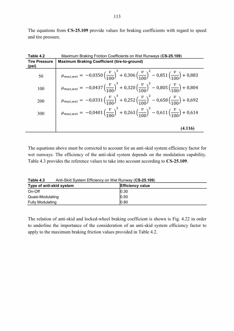
Indices for Aircraft Components .............................................................................................. 21
Other Indices ............................................................................................................................ 21
List of Abbreviations ................................................................................................................ 23
1 Introduction ......................................................................................................... 24
1.1 Motivation ........................................................................................................... 24
1.2 Definitions ........................................................................................................... 25
1.3 Project Objectives ................................................................................................ 27
1.4 Main Literature .................................................................................................... 28
1.5 Structure of the Report ......................................................................................... 29
2 Operational Hazards .......................................................................................... 31
2.1 Hazards from Wind, Rain, Snow and Ice ............................................................ 31
2.2 Definitions for Wet and Contaminated Runways ................................................ 32
2.3 Wet Runway Effects on Aircraft Performance .................................................... 33
2.3.1 Aquaplaning ......................................................................................................... 33
2.3.2 Acceleration .......................................................................................................... 35
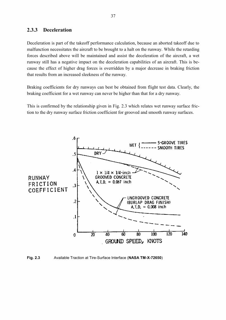
2.3.3 Deceleration ......................................................................................................... 37
2.3.4 Directional Stability ............................................................................................. 38
2.4 Responsibilities, Precautions and Airmanship ..................................................... 39
3 Certification Regulations ................................................................................... 40
3.1 Overview of Regulations for the Takeoff ............................................................ 40
3.2 Aircraft Speeds during Takeoff ........................................................................... 42
3.3 Distances in the Takeoff (Accelerate-Go) Case ................................................... 45
3.4 Distances in the Accelerate-Stop Case ................................................................. 48
3.5 Reaction Times after Critical Failure .................................................................... 50
3.6 Balanced Field Length ......................................................................................... 52
3.7 Takeoff Field Length ........................................................................................... 54
3.8 Consideration of Precipitation Drag on a Wet Runway ........................................ 55
4 Performance Calculation ................................................................................... 56
4.1 Liftoff Distance ................................................................................................... 56
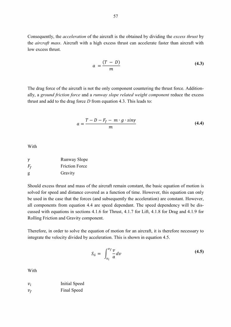
4.1.1 Equation of Motion – Derivation ........................................................................ 56
Page 9
9
4.1.2 Equation of Motion – Integration for Hand Calculations .................................... 58
4.1.3 Influence of Parameter Variation on Liftoff Distance ........................................... 60
4.1.4 Equation of Motion – Usage for Numerical Integration ..................................... 63
4.1.5 Density, Pressure and Reference Speeds in the Non-Standard Atmosphere ....... 66
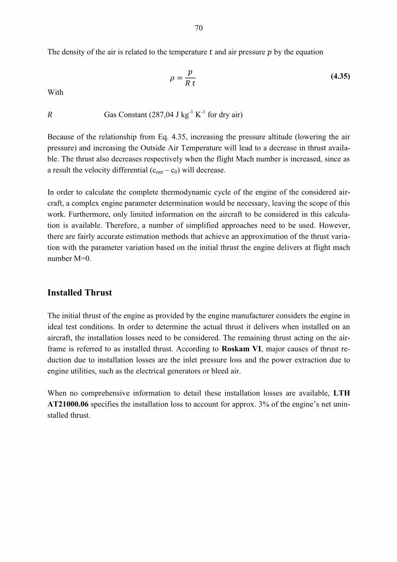
4.1.6 Thrust and Thrust Lapse ....................................................................................... 69
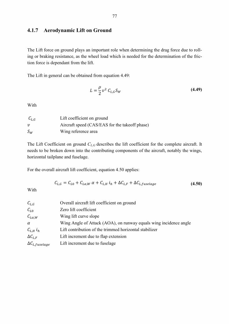
4.1.7 Aerodynamic Lift on Ground ............................................................................... 77
4.1.8 Aerodynamic Dragon Ground .............................................................................. 86
4.1.9 Rolling Friction and Gravity ................................................................................ 94
4.1.10 Displacement, Collision and Skin Friction Drag due to Water Spray ................. 97
4.2 Air Distance ....................................................................................................... 100
4.2.1 Rotation and Climb Trajectory ............................................................................ 102
4.2.2 Rotation and Climb Distances over Ground ........................................................ 104
4.3 Takeoff Distance – All Engines Operative ........................................................ 105
4.4 Takeoff Distance – One Engine Inoperative ...................................................... 106
4.4.1 Engine Failure Speed .......................................................................................... 106
4.4.2 Thrust and Drag after Engine Failure ................................................................ 107
4.5 Accelerate-Stop Distance .................................................................................. 111
4.5.1 Braking Force ..................................................................................................... 112
4.5.2 Drag and Lift Coefficients after Spoiler Deflection ........................................... 115
4.6 Balanced Field Length ........................................................................................ 118
4.7 Take-Off Field Length ....................................................................................... 120
4.8 Climb Weight Limit ............................................................................................ 121
5 Water Spray Impingement Drag ................................................................... 122
5.1 Literature Review .............................................................................................. 123
5.2 Spray Wave Types of Main and Front Wheels ................................................... 123
5.3 Spray Angle Assumptions .................................................................................. 124
5.4 Areas of the Aircraft Exposed to Water Spray .................................................... 130
5.5 Water Impingement Drag Force Determination ................................................. 132
6 Aircraft Parameters ......................................................................................... 138
6.1 General .............................................................................................................. 138
6.2 Geometry .......................................................................................................... 139
6.3 Mass ................................................................................................................... 140
6.4 Thrust ................................................................................................................... 141
6.5 Lift Coefficient .................................................................................................. 145
6.6 Drag Coefficient ................................................................................................ 148
6.7 Lift-to-Drag Ratio and Aircraft Polar .................................................................. 158
6.8 Braking Force ...................................................................................................... 160
6.9 Reaction Time Considerations ............................................................................ 162
6.10 Reference Speeds ................................................................................................ 164
6.11 Data for Precipitation Drag Determination ......................................................... 168
Page 10
10
7 Numerical Takeoff Simulation ........................................................................ 169
7.1 Simulation Concept ............................................................................................ 170
7.2 Verification and Calibration ............................................................................... 171
7.3 Simulation Architecture ...................................................................................... 173
7.4 Simulation in Octave and MATLAB ................................................................ 174
7.4.1 Main Function .................................................................................................... 174
7.4.2 Outer Loop - Distance Integration Functions ..................................................... 175
7.4.3 Inner Loop –Acceleration and Deceleration Functions ....................................... 178
8 Simulation Results and Result Comparison .................................................. 179
8.1 Simulation Results ............................................................................................... 179
8.1.1 Useful Result Range ............................................................................................ 181
8.1.2 Simulation Results for Wet Runway, No Stores ................................................. 182
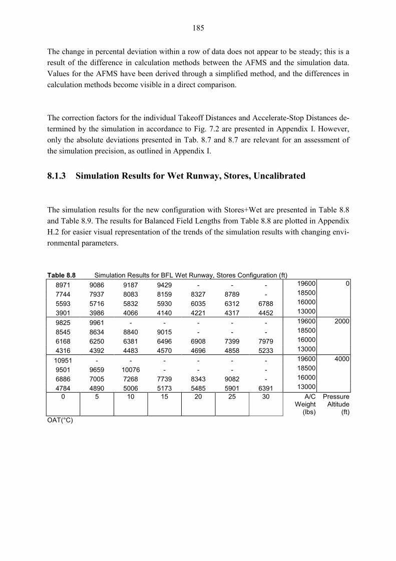
8.1.3 Simulation Results for Wet Runway, Stores, Uncalibrated ................................ 185
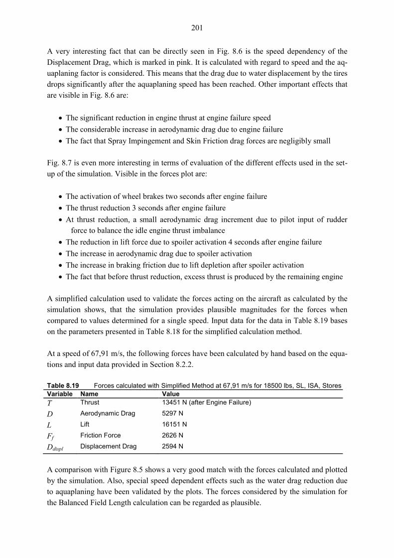
8.1.4 Simulation Results with Applied Calibration, Wet Runway, Stores ................... 186
8.2 Results Cross-Correlation ................................................................................... 188
8.2.1 Comparison of Simulation Results with existing Certified Data ........................ 188
8.2.2 Comparison of Takeoff Distance from Simulation with Simplified Method ...... 194
8.3 Validation of Main Forces during Takeoff Roll with Simplified Calculation .... 199
9 Validation of Simulation Results ..................................................................... 202
9.1 Possible Error Sources and Rectification ............................................................ 202
9.1.1 Programming Errors ............................................................................................ 202
9.1.2 Model Inaccuracies .............................................................................................. 203
9.1.3 Test Methods for Analysis .................................................................................. 203
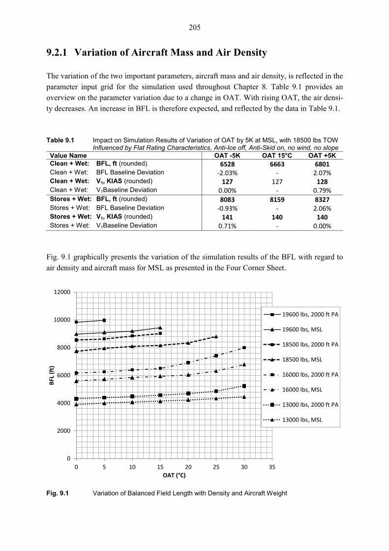
9.2 Parameter Variation Effects and Influence on Simulation Results ..................... 204
9.2.1 Variation of Aircraft Mass and Air Density ........................................................ 205
9.2.2 Variation of Aerodynamic Parameters ................................................................ 207
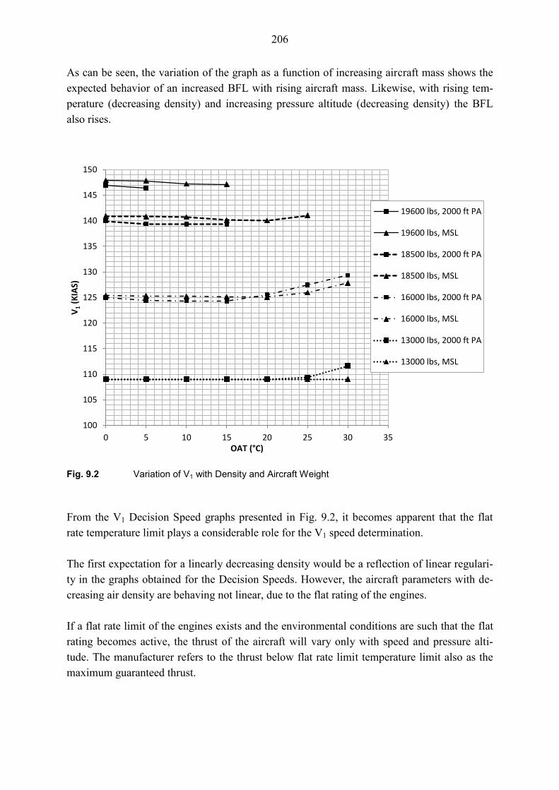
9.2.3 Variation of Thrust Parameters ........................................................................... 210
9.2.4 Variation of Precipitation Drag Force ................................................................. 211
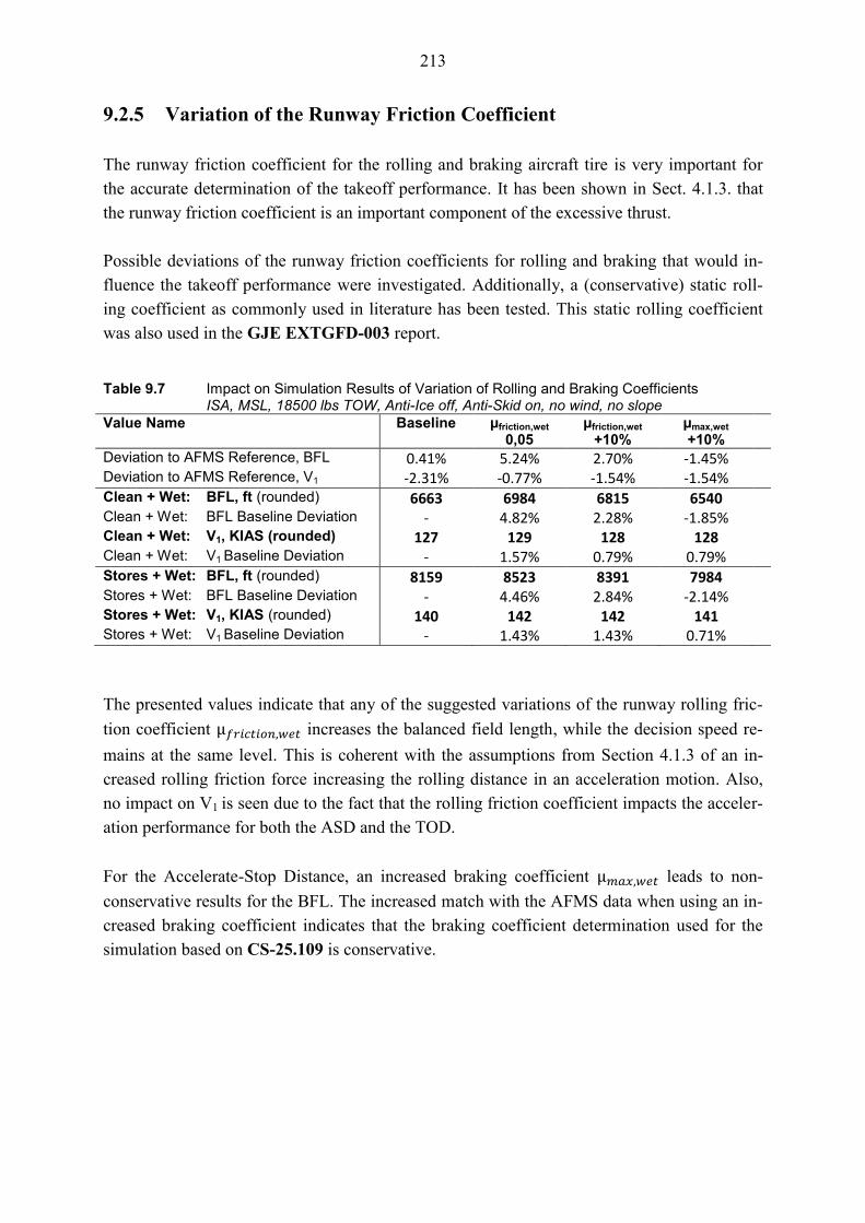
9.2.5 Variation of the Runway Friction Coefficient ..................................................... 213
9.2.6 Variation of the Wind and Runway Slope ........................................................... 214
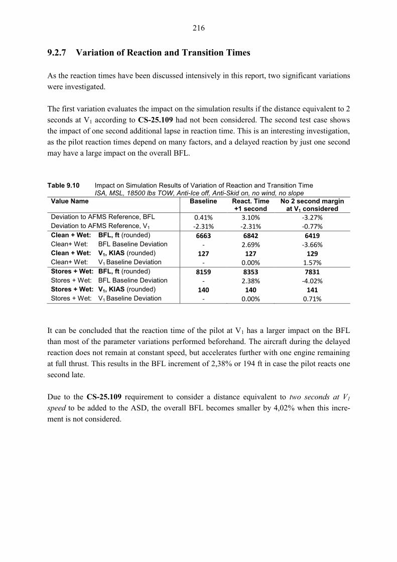
9.2.7 Variation of Reaction and Transition Times ....................................................... 216
10 Conclusions ....................................................................................................... 217
10.1 Conclusion on Modeling Precision ..................................................................... 217
10.2 Correlation of Expected and Actual Results ....................................................... 218
10.3 Calculation Approach Validation ........................................................................ 219
Page 11
11
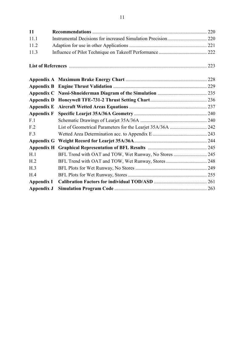
11 Recommendations ............................................................................................. 220
11.1 Instrumental Decisions for increased Simulation Precision ................................ 220
11.2 Adaption for use in other Applications ............................................................... 221
11.3 Influence of Pilot Technique on Takeoff Performance ....................................... 222
List of References ................................................................................................................ 223
Appendix A Maximum Brake Energy Chart .................................................................. 228
Appendix B Engine Thrust Validation ............................................................................ 229
Appendix C Nassi-Shneiderman Diagram of the Simulation ........................................ 235
Appendix D Honeywell TFE-731-2 Thrust Setting Chart .............................................. 236
Appendix E Aircraft Wetted Areas Equations ............................................................... 237
Appendix F Specific Learjet 35A/36A Geometry ........................................................... 240
F.1 Schematic Drawings of Learjet 35A/36A ...................................................... 240
F.2 List of Geometrical Parameters for the Learjet 35A/36A .............................. 242
F.3 Wetted Area Determination acc. to Appendix E ............................................ 243
Appendix G Weight Record for Learjet 35A/36A ........................................................... 244
Appendix H Graphical Representation of BFL Results ................................................ 245
H.1 BFL Trend with OAT and TOW, Wet Runway, No Stores ........................... 245
H.2 BFL Trend with OAT and TOW, Wet Runway, Stores ................................. 248
H.3 BFL Plots for Wet Runway, No Stores .......................................................... 249
H.4 BFL Plots for Wet Runway, Stores ................................................................ 255
Appendix I Calibration Factors for individual TOD/ASD ........................................... 261
Appendix J Simulation Program Code ........................................................................... 263
Page 12
12
List of Figures
Fig. 2.1 Effect of Speed on Water Drag Coefficients ......................................................... 34
Fig. 2.2 Precipitation Drag Forces due to Contaminated Runway Conditions ................... 35
Fig. 2.3 Available Traction at Tire-Surface Interface ......................................................... 37
Fig. 3.1 Takeoff Speeds and ground distances in AEO condition ...................................... 43
Fig. 3.2 Takeoff in OEI Conditions .................................................................................... 46
Fig. 3.3 Takeoff Run and Takeoff Distance with Clearway considered ............................ 47
Fig. 3.4 TORA, ASDA and TODA with Clear- and Stopway available ............................ 48
Fig. 3.5 Aborted Takeoff with Critical Engine Failure ...................................................... 49
Fig. 3.6 V1 and VEF Interdependence &Time Delay for Retardation Device Activation .. 51
Fig. 3.7 Balanced Field Length as Equal Distance of ASD and TOD ................................ 52
Fig. 3.8 Example Balanced Field Length – TOD and ASD Curve Intersection ................. 53
Fig. 4.1 Distance and Velocity for Acceleration with Decreasing Excess Thrust .............. 65
Fig. 4.2 Distance and Velocity for Deceleration with Negative Excess
Thrust and delayed Retardation Device Activation .............................................. 65
Fig. 4.3 Thrust Variation with Pressure Altitude, Mach Number and OAT, flat rated ...... 69
Fig. 4.4 Different Approaches to compare Mach Number Dependency of Thrust ............ 73
Fig. 4.5 Thrust Flat Rating for different Pressure Altitudes,
TFE-731-2 Turbofan Engine ................................................................................. 76
Fig. 4.6 Determination of the Mach Correction Factor for Zero Lift Angle of Attack ...... 80
Fig. 4.7 Determination of the Wing Twist to Zero Lift Angle of Attack Ratio .................. 80
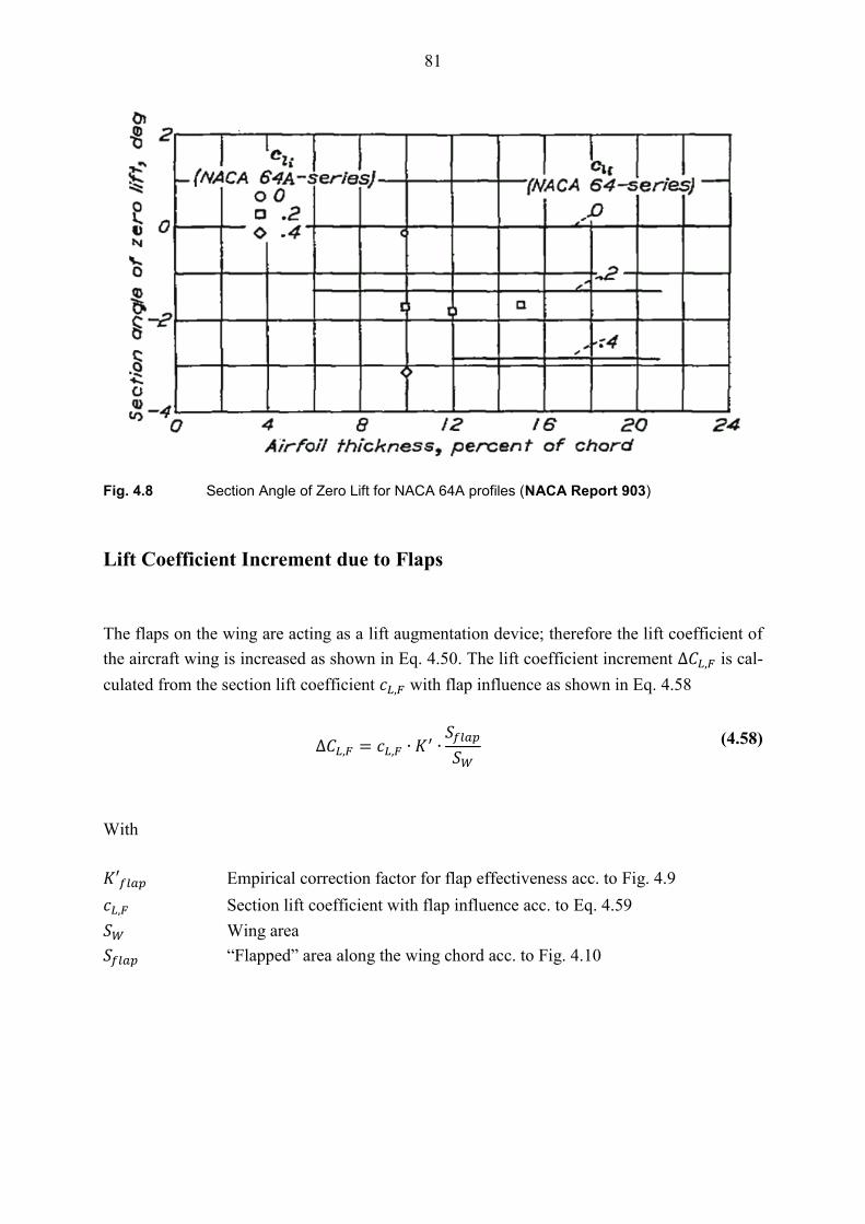
Fig. 4.8 Section Angle of Zero Lift for NACA 64A profiles ............................................. 81
Fig. 4.9 Empirical Correction Factor for Flap Effectiveness .............................................. 82
Fig. 4.10 Flapped Area of the Wing along the Chord Line .................................................. 82
Fig. 4.11 Lift Effectiveness Parameter by Flap Deflection Angle ....................................... 83
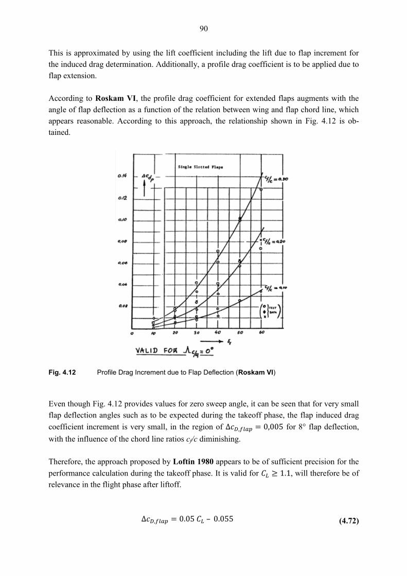
Fig. 4.12 Profile Drag Increment due to Flap Deflection ..................................................... 90
Fig. 4.13 Gear Drag Coefficient as a Function of the Flap Deflection Angle ...................... 91
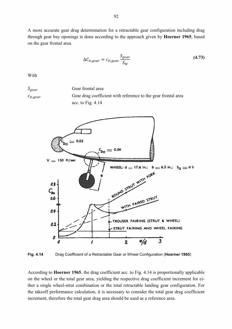
Fig. 4.14 Drag Coefficient of a Retractable Gear or Wheel Configuration .......................... 92
Fig. 4.15 Stores Configuration in External Rack or on Pylon .............................................. 93
Fig. 4.16 Runway Slope, Friction and Downhill Force in their Relation to each other ....... 94
Fig. 4.17 Dynamic Surface Rolling Coefficients for a Small Business Jet .......................... 96
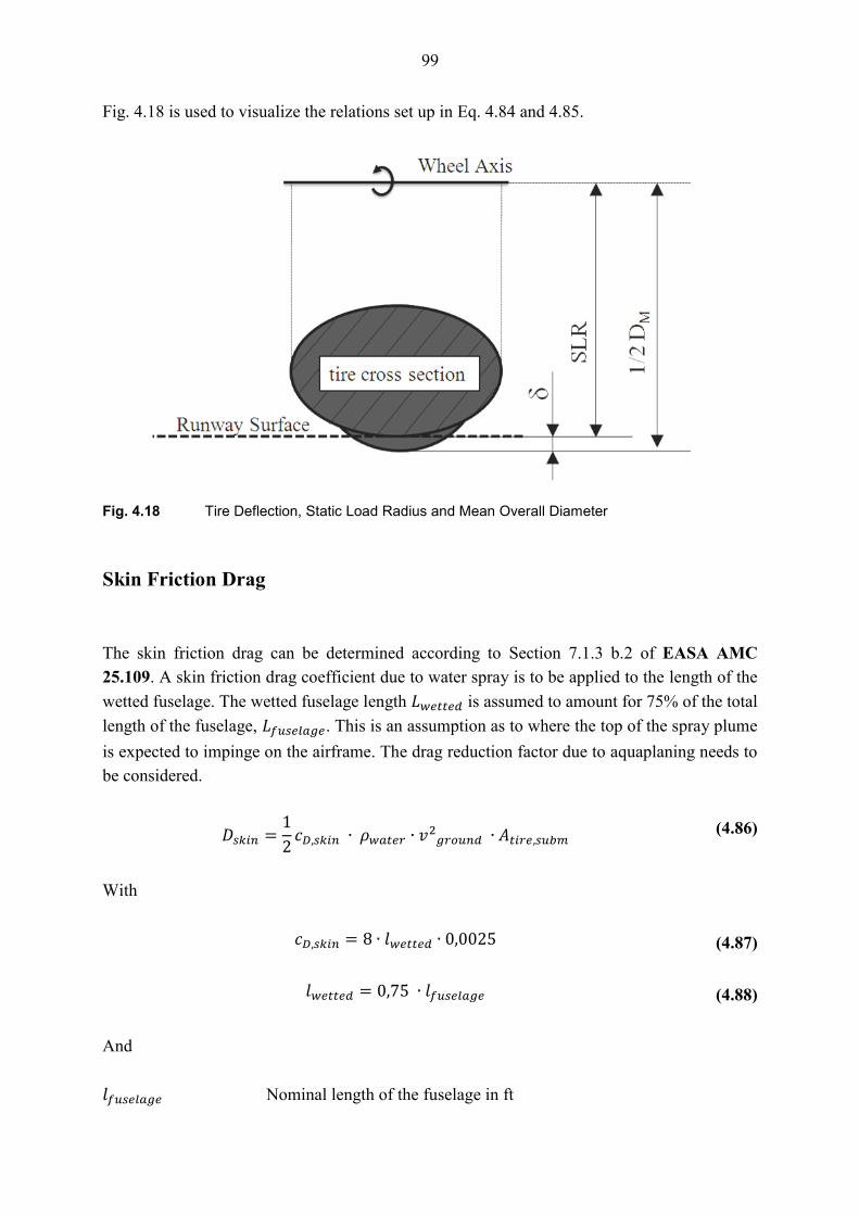
Fig. 4.18 Tire Deflection, Static Load Radius and Mean Overall Diameter ........................ 99
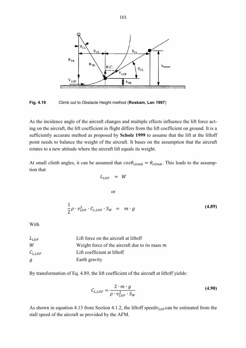
Fig. 4.19 Climb out to Obstacle Height Method ................................................................ 101
Fig. 4.20 Forces acting on the Aircraft in Engine Failure Case, Wings Leveled ............... 107
Fig. 4.21 Effective VTP Aspect Ratio of the Fin for a T-tail configuration ....................... 110
Fig. 4.22 Braking Friction Coefficient on Wet Runway, Maximum, Anti-Skid
and Locked Wheel ............................................................................................... 114
Fig. 4.23 Basic Braking Coefficients for Wet Runways .................................................... 115
Page 13
13
Fig. 4.24 Turbulent Flow behind a deflected Spoiler ......................................................... 116
Fig. 4.25 Extended Spoiler Geometry Upper Wing ........................................................... 117
Fig. 5.1 MTR-101 Pod installed under the wing of a Learjet 35A/36A ........................... 122
Fig. 5.2 Bow and side wave of spray plume ..................................................................... 124
Fig. 5.3 Spray Angle with regard to Aircraft and Aquaplaning Speed ............................. 125
Fig. 5.4 Chined Tire Deflection Spray Angle ................................................................... 127
Fig. 5.5 Learjet 35A/36A GFD Configuration Front Wheel Tire with shines ................. 128
Fig. 5.6 Overlay “CRspray” Calculation and Learjet 35A/36A ....................................... 129
Fig. 5.7 Overlay NASA TP-2718 Test Run and Learjet 35A/36A ................................... 129
Fig. 5.8 Under-Wing Store MTR-101 Dimensions .......................................................... 130
Fig. 5.9 Gear Geometry Front View Learjet 35A/36A, Measurements taken from
the Aircraft .......................................................................................................... 131
Fig. 5.10 NASA Spray Test Vehicle .................................................................................. 132
Fig. 5.11 NASA Spray Pattern of Test Run 33, Identification of Maximum
Spray Intensity Area ............................................................................................ 133
Fig. 6.1 Cutaway Picture of the Gates Learjet 35A/36A .................................................. 138
Fig. 6.2 Installed Thrust Variations with Pressure Altitude and OAT for
TFE731-2B-2 Engine .......................................................................................... 141
Fig. 6.3 Flat Rate Temperature limit with regard to Pressure altitude ............................. 144
Fig. 6.4 Plot of Lift Coefficient on Ground as used for the numerical calculation .......... 146
Fig. 6.5 Drag Coefficients Simulation for Learjet 35A/36A with Stores, Takeoff Case . 149
Fig. 6.6 Drag Coefficients Simulation for Learjet 35A/36A with Stores,
Accelerate-Stop Case .......................................................................................... 150
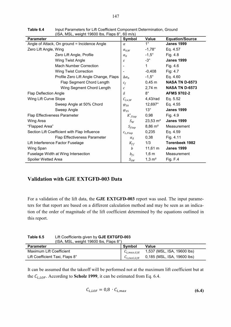
Fig. 6.7 Variation of Windmilling Drag with Mach Number ........................................... 154
Fig. 6.8 Variation of Drag Coefficient due to Asymmetrical Flight Condition
with Speed ........................................................................................................... 155
Fig. 6.9 Aircraft Polar, Learjet 35A/36A acc. to Parameter Estimations,
Varied Configurations ......................................................................................... 159
Fig. 6.10 Braking Friction Coefficient Dry Runway for a Learjet 35A/36A ..................... 160
Fig. 6.11 Braking Coefficient used in Simulation for the Learjet 35A, 36A ..................... 161
Fig. 6.12 Reaction Times and Aircraft Retardation with Engine Failure at t=0 ................. 163
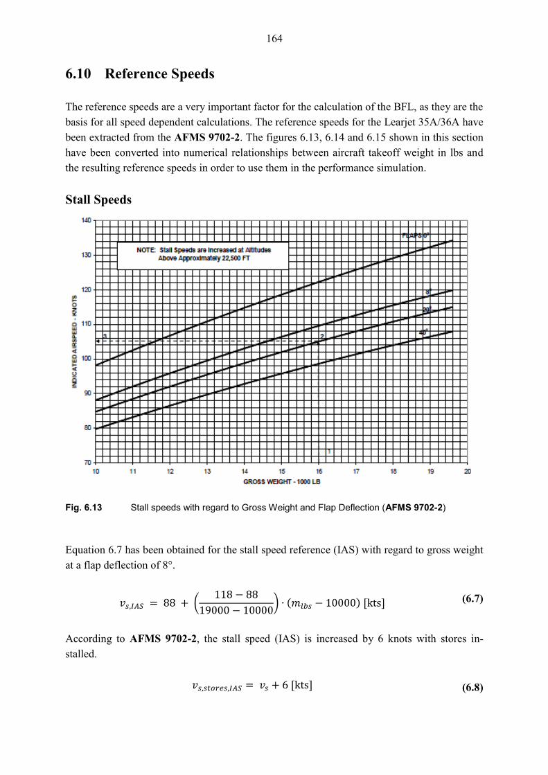
Fig. 6.13 Stall Speeds with regard to Gross Weight and Flap Deflection .......................... 164
Fig. 6.14 Rotation Speeds with regard to Gross Weight and Store Installation ................. 165
Fig. 6.15 Safe Climb speeds with regard to Gross Weight and Store Installation ............. 166
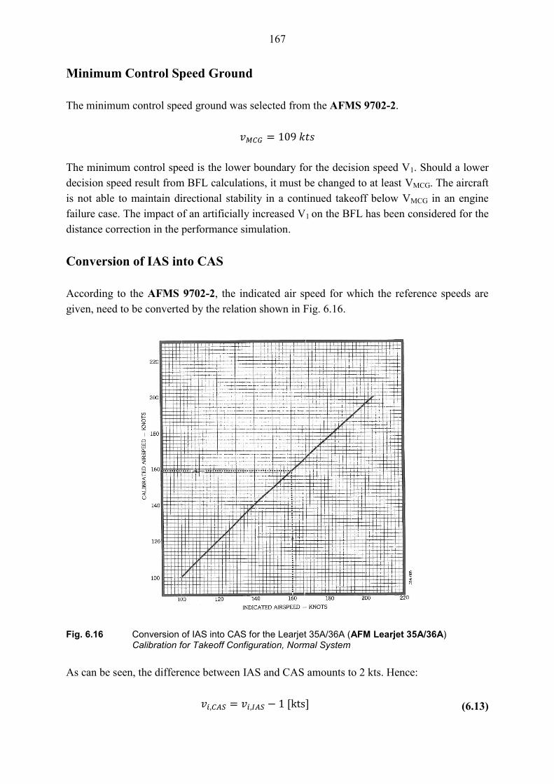
Fig. 6.16 Conversion of IAS into CAS for the Learjet 35A/36A ....................................... 167
Fig. 7.1 Four-Corner Sheet of existing certification data ............................................... 171
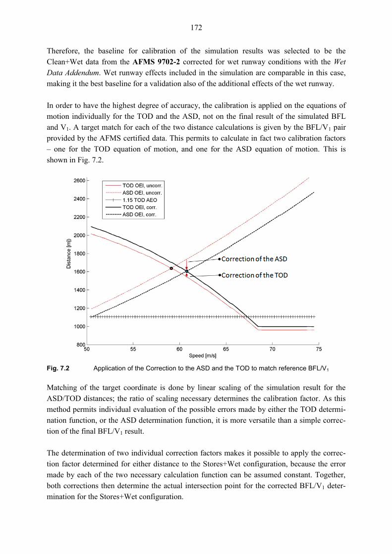
Fig. 7.2 Application of the Correction to the ASD and the TOD to match
Reference BFL/V1 .............................................................................................. 172
Fig. 7.3 Overall Simulation Architecture and Calibration Concept, Simplified .............. 173
Page 14
14
Fig. 7.4 Overall Accelerate-Stop Distance Function Architecture ................................... 176
Fig. 7.5 Overall Takeoff Distance Function Architecture ................................................ 177
Fig. 8.1 Precision of the Simulation with regard to Time Step Width ............................. 180
Fig. 8.2 Comparison of Simulation Results for BFL with and without Calibration ......... 187
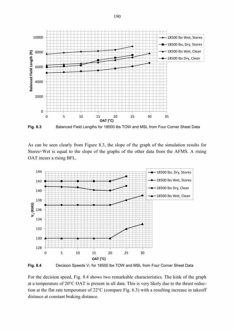
Fig. 8.3 Balanced Field Lengths for 18500 lbs TOW and MSL from Four Corner
Sheet Data ............................................................................................................ 190
Fig. 8.4 Decision Speeds V1 for 18500 lbs TOW and MSL from Four Corner
Sheet Data ............................................................................................................ 190
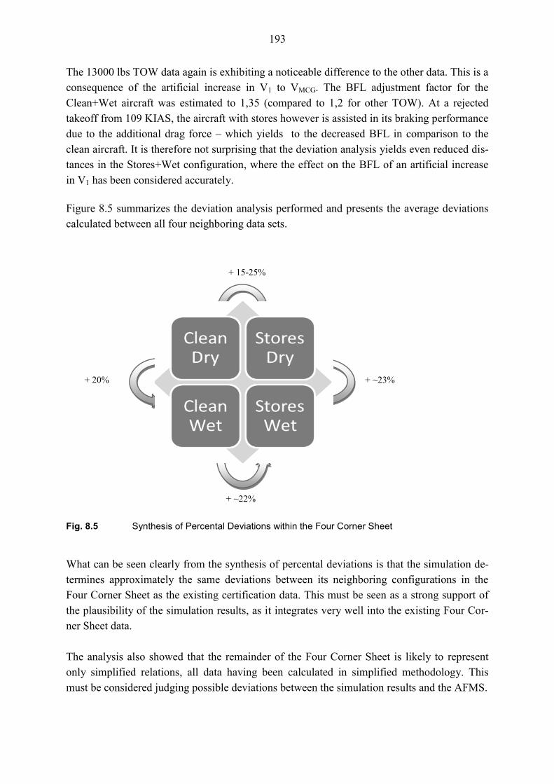
Fig. 8.5 Synthesis of Percental Deviations within the Four Corner Sheet ....................... 193
Fig. 8.6 Forces on the Aircraft during Acceleration with Engine Failure ........................ 200
Fig. 8.7 Forces on the Aircraft during Deceleration after Engine Failure ........................ 200
Fig. 9.1 Variation of Balanced Field Length with Density and Aircraft Weight ............. 205
Fig. 9.2 Variation of V1 with Density and Aircraft Weight .............................................. 206
Fig. A.1 Maximum Brake Energy Chart ........................................................................... 228
Fig. B.1 Validation of GJE Test Data with Academic Thrust Model for MSL, ISA ........ 229
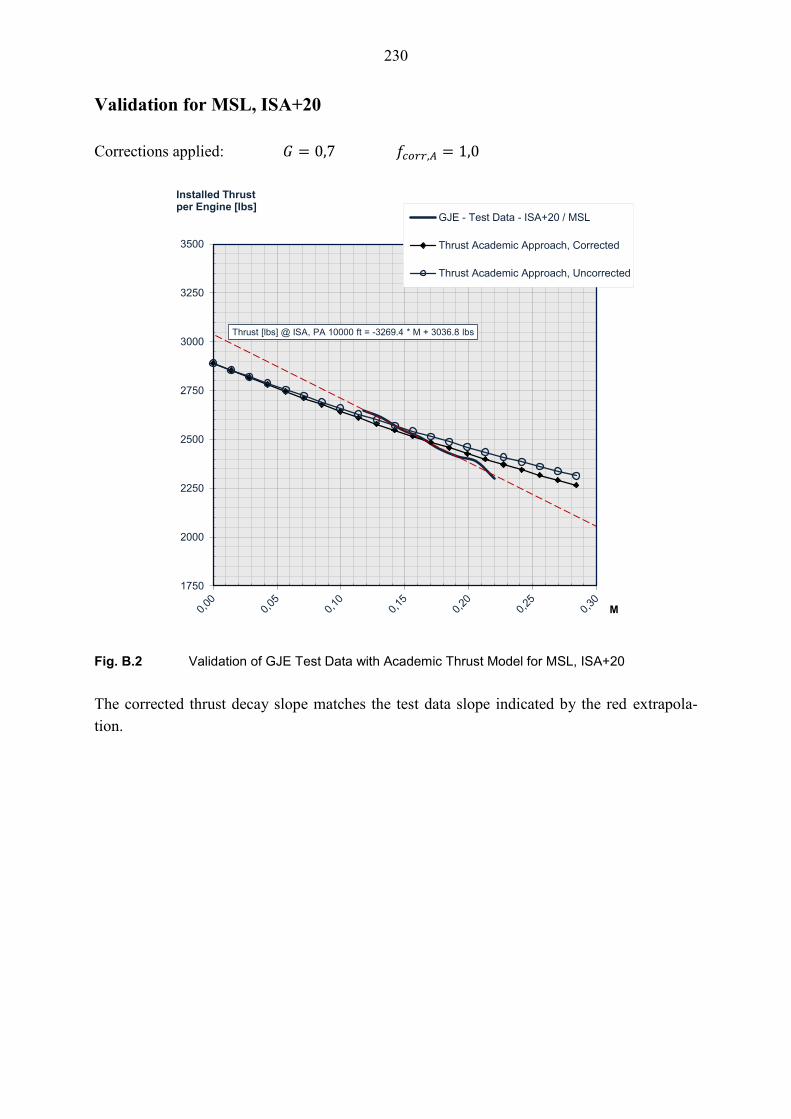
Fig. B.2 Validation of GJE Test Data with Academic Thrust Model for MSL, ISA+20 .. 230
Fig. B.3 Validation of GJE Test Data with Academic Thrust Model for 5000 ft, ISA ..... 231
Fig. B.4 Validation of GJE Test Data with Academic Thrust Model for 5000 ft,ISA+20 232
Fig. B.5 Validation of GJE Test Data with Academic Thrust Model for 10000 ft, ISA ... 233
Fig. B.6 Estimation of a Correction Factor for ‘A’ in the Academic Thrust Model ......... 234
Fig. C.1 Nassi-Shneiderman Diagram of the Simulation .................................................. 235
Fig. D1 Learjet TFE-731-2 Thrust Setting Chart ............................................................. 236
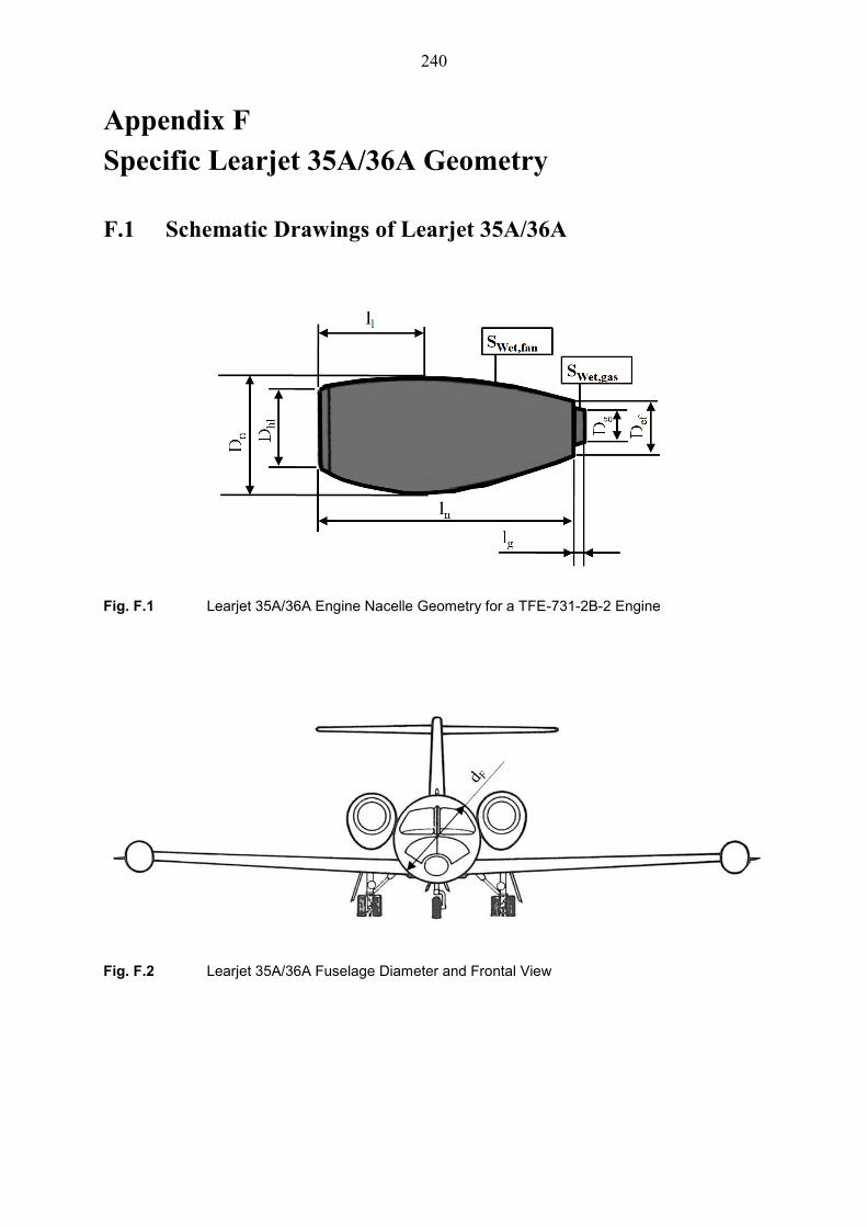
Fig. F.1 Learjet 35A/36A Engine Nacelle Geometry for a TFE-731-2B-2 Engine .......... 240
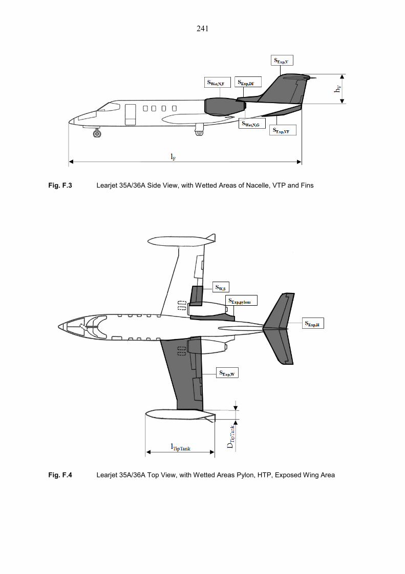
Fig. F.2 Learjet 35A/36A Fuselage Diameter and Frontal View ...................................... 240
Fig. F.3 Learjet 35A/36A Side View, with Wetted Areas of Nacelle, VTP and Fins ...... 241
Fig. F.4 Learjet 35A/36A Top View, with Wetted Areas Pylon, HTP, Exposed
Wing Area ........................................................................................................... 241
Fig. G.1 Weight Record for Learjet 35A/36A in GFD Configuration .............................. 244
Fig. H.1 Simulation Results for BFL, Wet Runway, No Stores, 19600 lbs TOW ............ 245
Fig. H.2 Simulation Results for BFL, Wet Runway, No Stores, 18500 lbs TOW ............ 245
Fig. H.3 Simulation Results for BFL, Wet Runway, No Stores, 16000 lbs TOW ............ 246
Fig. H.4 Simulation Results for BFL, Wet Runway, No Stores, 13000 lbs TOW ............ 246
Page 15
15
Fig. H.5 Simulation Results for BFL, Wet Runway, Stores, 19600 lbs TOW .................. 247
Fig. H.6 Simulation Results for BFL, Wet Runway, Stores, 18500 lbs TOW .................. 247
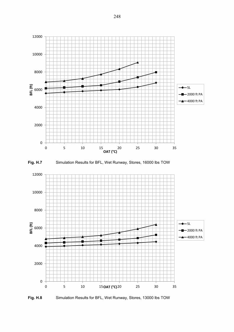
Fig. H.7 Simulation Results for BFL, Wet Runway, Stores, 16000 lbs TOW .................. 248
Fig. H.8 Simulation Results for BFL, Wet Runway, Stores, 13000 lbs TOW .................. 258
Fig. H.9 Balanced Field Length Plot, 15°C OAT, MSL, 19600 lbs TOW, NoStores ....... 249
Fig. H.10 Balanced Field Length Plot, 10°C OAT, 2000 ft PA, 19600 lbs TOW,NoStores249
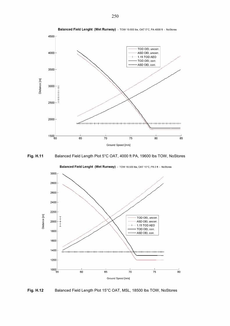
Fig. H.11 Balanced Field Length Plot 5°C OAT, 4000 ft PA, 19600 lbs TOW, NoStores 250
Fig. H.12 Balanced Field Length Plot 15°C OAT, MSL, 18500 lbs TOW, NoStores ........ 250
Fig. H.13 Balanced Field Length Plot 10°C OAT, 2000 ft PA, 18500 lbs TOW, NoStores251
Fig. H.14 Balanced Field Length Plot 5°C OAT, 4000 ft PA, 18500 lbs TOW, NoStores 251
Fig. H.15 Balanced Field Length Plot 15°C OAT, MSL, 16000 lbs TOW, NoStores ........ 252
Fig. H.16 Balanced Field Length Plot 10°C OAT, 2000 ft PA, 16000 lbs TOW, NoStores252
Fig. H.17 Balanced Field Length Plot 5°C OAT, 4000 ft PA, 16000 lbs TOW, NoStores 253
Fig. H.18 Balanced Field Length Plot 15°C OAT, MSL, 13000 lbs TOW, NoStores ........ 253
Fig. H.19 Balanced Field Length Plot 10°C OAT, 2000 ft PA, 13000 lbs TOW, NoStores254
Fig. H.20 Balanced Field Length Plot 5°C OAT, 4000 ft PA, 13000 lbs TOW, NoStores 254
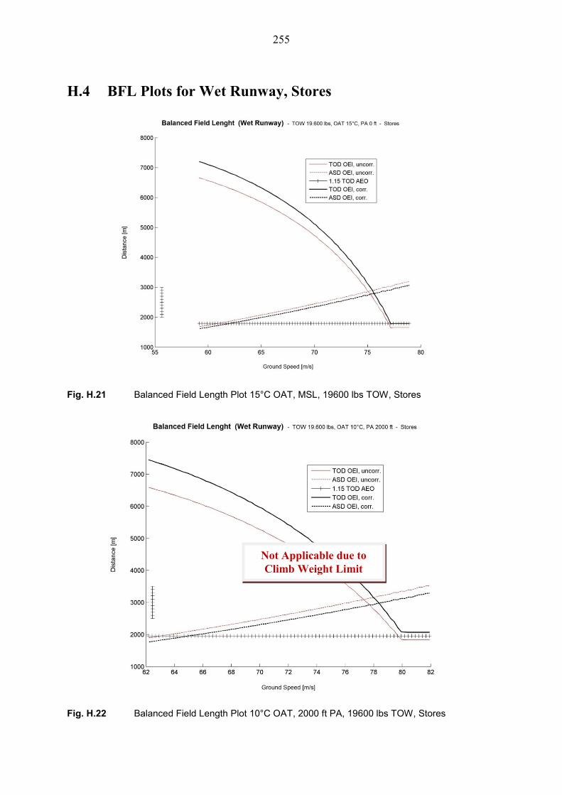
Fig. H.21 Balanced Field Length Plot, 15°C OAT, MSL, 19600 lbs TOW, Stores ............ 255
Fig. H.22 Balanced Field Length Plot, 10°C OAT, 2000 ft PA, 19600 lbs TOW, Stores .. 255
Fig. H.23 Balanced Field Length Plot 5°C OAT, 4000 ft PA, 19600 lbs TOW, Stores ..... 256
Fig. H.24 Balanced Field Length Plot 15°C OAT, MSL, 18500 lbs TOW, Stores ............. 256
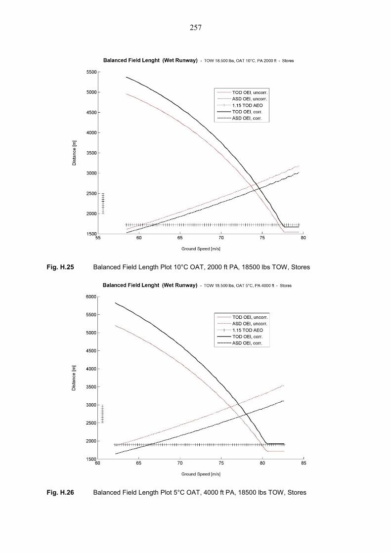
Fig. H.25 Balanced Field Length Plot 10°C OAT, 2000 ft PA, 18500 lbs TOW, Stores ... 257
Fig. H.26 Balanced Field Length Plot 5°C OAT, 4000 ft PA, 18500 lbs TOW, Stores ..... 257
Fig. H.27 Balanced Field Length Plot 15°C OAT, MSL, 16000 lbs TOW, Stores ............. 258
Fig. H.28 Balanced Field Length Plot 10°C OAT, 2000 ft PA, 16000 lbs TOW, Stores ... 258
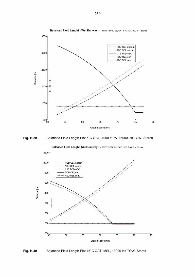
Fig. H.29 Balanced Field Length Plot 5°C OAT, 4000 ft PA, 16000 lbs TOW, Stores ..... 259
Fig. H.30 Balanced Field Length Plot 15°C OAT, MSL, 13000 lbs TOW, Stores ............. 259
Fig. H.31 Balanced Field Length Plot 10°C OAT, 2000 ft PA, 13000 lbs TOW, Stores ... 260
Fig. H.32 Balanced Field Length Plot 5°C OAT, 4000 ft PA, 13000 lbs TOW, Stores ..... 260
Fig. I.1 Balanced Field Length and V1 in dependence of individual Correction Factors 262
Page 16
16
List of Tables
Table 4.1 Static Surface Rolling Coefficients, from Scholz 1999 ............................... 95
Table 4.2 Maximum Braking Friction Coefficients on Wet Runways ...................... 113
Table 4.3 Anti-Skid System Efficiency on Wet Runway .......................................... 113
Table 4.4 Minimum Climb Gradients Specified by CS-25 ........................................ 121
Table 6.1 Wing Parameters for Aerodynamic Analysis ............................................ 140
Table 6.2 Honeywell TFE-731-2-2B Engine Characteristics .................................... 141
Table 6.3 Lift Coefficient and Lift Coefficient Components ..................................... 145
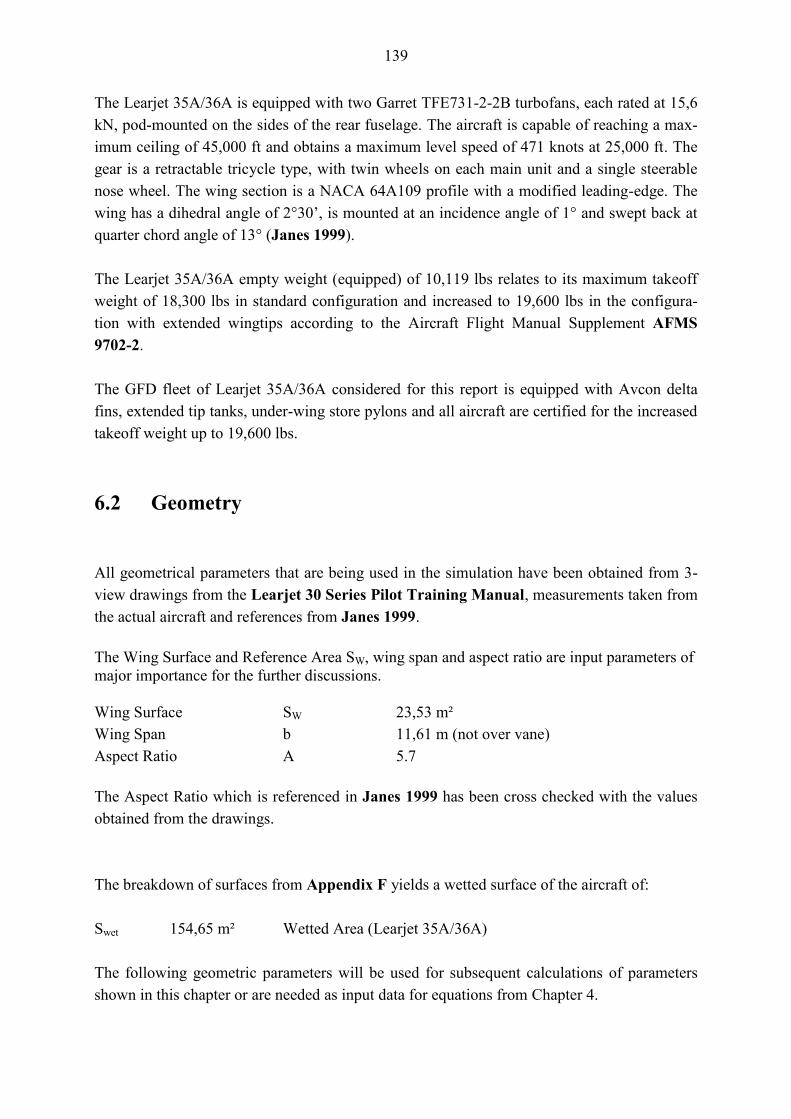
Table 6.4 Input Parameters for Lift Coefficient Component Determination, Ground 147
Table 6.5 Lift Coefficients given by GJE EXTGFD-003 .......................................... 147
Table 6.6 Drag Coefficients used in Takeoff Perf. Simulation, Stores installed ....... 148
Table 6.7 Profile Drag Coefficient Breakdown according to Roskam 1989 ............. 151
Table 6.8 Induced Drag Coefficient Calculation Parameters ..................................... 152
Table 6.9 Store Drag Coefficient Increment Calculation Parameters ........................ 153
Table 6.10 Gear Drag Coefficient Increment Calculation Parameters ........................ 153
Table 6.11 Windmilling Drag Coefficient Increment Calculation Parameters ............ 154
Table 6.12 Asymmetrical Flight Condition Drag Coefficient Increment
Calculation Parameters .............................................................................. 156
Table 6.13 Spoiler Deflection Condition Drag Coefficient Increment
Calculation Parameters .............................................................................. 157
Table 6.14 Drag Coefficients used in GJE EXTGFD-003 Takeoff Performance
Simulation .................................................................................................. 157
Table 6.15 Glide Ratio of Learjet 35A/36A as determined from
Parameter Estimation, AEO ....................................................................... 158
Table 6.16 Calculation Parameters for Precipitation Drag, Learjet 35A/36A ............. 168
Table 6.17 Learjet 35A/36A Tire Data ........................................................................ 168
Table 8.1 Comparison of Time-Step-Width Resolution Deviations in
Simulation Results ..................................................................................... 180
Table 8.2 Climb Weight Limit for Learjet 35A/36A in Extended Tip
Tank Configuration ................................................................................... 181
Table 8.3 Climb Weight Limit for Learjet 35A/36A in Extended Tip Tank
and Dual MTR-101 Stores Configuration ................................................. 181
Table 8.4 Simulation Results for BFL Wet Runway, No Stores Configuration (ft) .. 182
Table 8.5 Simulation Results for V1 Wet Runway, No Stores Configuration .......... 183
Table 8.6 Deviation of BFL calculated by the Simulation to AFM
Reference Data for Clean+Wet .................................................................. 184
Table 8.7 Deviation of V1 calculated by the Simulation to AFM
Reference Data for Clean+Wet .................................................................. 184
Table 8.8 Simulation Results for BFL Wet Runway, Stores Configuration (ft) ........ 185
Table 8.9 Simulation Results for V1 Wet Runway, Stores Configuration ................ 186
Page 17
17
Table 8.10 Simulation Results for BFL Wet Runway, Stores Configuration (ft),
Applied Calibration ................................................................................... 186
Table 8.11 Simulation Results for V1 Wet Runway, Stores Configuration,
Applied Calibration ................................................................................... 187
Table 8.12 Four Corner Sheet of BFL at SL with Simulation Results Stores+Wet ... 189
Table 8.13 Four Corner Sheet of V1 at SL with Simulation Results .......................... 189
Table 8.14 Deviation of BFL from Clean+Dry towards Clean+Wet values ............... 191
Table 8.15 Deviation of BFL from Clean+Dry towards Stores+Dry values ............... 191
Table 8.16 Deviation of BFL from Stores+Dry towards Stores+Wet values .............. 192
Table 8.17 Deviation of BFL from Clean+Wet towards Stores+Wet values .............. 192
Table 8.18 Input Parameters for the hand calculation ................................................. 196
Table 8.19 Forces calculated with Simplified Method at 67,91 m/s for 18500 lbs ..... 201
Table 9.1 Impact on Simulation Results of Variation of OAT by 5K at MSL,
with 18500 lbs TOW .................................................................................. 205
Table 9.2 Impact on Simulation Results of Variation of CL,G by 10%....................... 208
Table 9.3 Impact on Simulation Results of Variation of CD,TO by 10% ..................... 209
Table 9.4 Impact on Simulation Results of Variation of Installed Thrust ................. 210
Table 9.5 Impact on Simulation Results of Variation of Spray Impingement Drag .. 211
Table 9.6 Impact on Simulation Results of Variation of Precipitation
Displacement Drag ..................................................................................... 212
Table 9.7 Impact on Simulation Results of Variation of Rolling and
Braking Coefficients .................................................................................. 213
Table 9.8 Impact on Simulation Results of Variation of Wind Speed and
Runway Slope, 18500 lbs........................................................................... 214
Table 9.9 Impact on Simulation Results of Variation of Wind Speed and
Runway Slope, 16000 lbs........................................................................... 214
Table 9.10 Impact on Simulation Results of Variation of Reaction and
Transition Time .......................................................................................... 216
Table 10.1 Synthesis of Input Parameter Variation Impact on Simulation
Results based on a test case, 185000 lbs TOW, ISA, SL, Stores+Wet ...... 217
Table F.1 Measurements taken from the Learjet 35A/36A ........................................ 242
Table F.2 Exposed areas of the Learjet 35A/36A as shown in Appendix E .............. 242
Table F.3 Wetted Areas for the Learjet 35A/36A based on the Exposed Area
Calculation Method .................................................................................... 243
Table I.1 Calibration Factor on the TOD, Comparison of Simulation Result to
AFMS Data ................................................................................................ 261
Table I.2 Calibration Factor on the ASD, Comparison of Simulation Result to
AFMS Data ................................................................................................ 261
Page 18
18
List of Symbols
Speed of sound in standard conditions(340.294 m/s)
Acceleration in z-axis of the aircraft during rotation
Acceleration
Engine inlet area
Aspect ratio
Zero lift angle of attack change due to flap deflection
Tire frontal area submerged in water
Effective (aerodynamic) aspect ratio of the VTP
Wing span
VTP span
Effective tire width
Fuselage width at wing intersection
BPR Bypass-Ratio of the engine
Outflow speed of the engine
Wing chord length
Flap segment chord length
Chord at Wing Tip
Chord at Wing Root
Chord of the Spoiler
Drag coefficient
Drag coefficient increment
Lift Coefficient Aircraft
Lift coefficient airfoil/section lift coefficient
Lift coefficient per area
Zero lift coefficient
Wing lift curve slope
Profile lift coefficient
Lift contribution of the trimmed horizontal stabilizer
Lift increment
VTP profile lift coefficient after rudder deflection
Specific engine temperature parameters
Equivalent skin friction coefficient
Drag
Rim flange outer diameter
Mean overall tire diameter
Contaminant depth
Percental tire deflection,
Engine inlet diameter
Page 19
19
Lift-to-Drag Ratio
Brake Energy
Restitution Coefficient
Oswald factor
Correction/Adaption factor
Force
g Gravity
G Gas generator function
H Pressure altitude in ft
Wing-to-ground distance
Screen Height
Transition Height
Incidence angle horizontal stabilizer
Empirical correction factor for aerodynamic effectiveness
Spray angle factor
Lift interference factor
Store interference factor
Correction factor for VTP sweep
Temperature gradient with altitude
Length
Flight mach number
Mass
Mass flow
Normal Force on Wheel Strut
Number of tires
Barometric pressure
ISA standard ambient pressure
Ratio of total displaced water vs. water impinging on exposed area
Gas Constant
Radius of bow shaped rotation trajectory
Distance over ground
Geometrical reference area
SLR Static Load Radius
T Thrust
Static Thrust
ISA standard temperature
Temperature at test conditions
ISA temperature deviation
Thickness of the wing
Ground lift coefficient estimate
Fluid particle velocity
Page 20
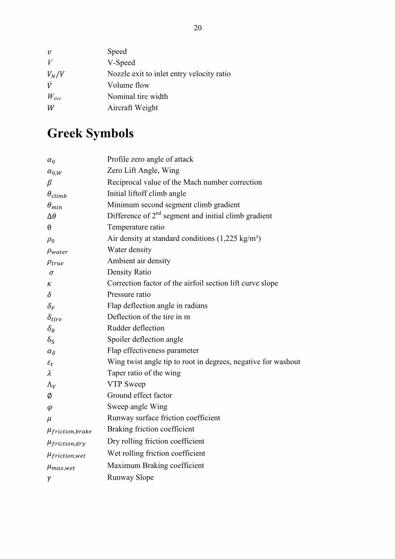
20
Speed
V V-Speed
Nozzle exit to inlet entry velocity ratio
Volume flow
Wtire Nominal tire width
Aircraft Weight
Greek Symbols
Profile zero angle of attack
Zero Lift Angle, Wing
Reciprocal value of the Mach number correction
Initial liftoff climb angle
Minimum second segment climb gradient
Difference of 2nd
segment and initial climb gradient
Temperature ratio
Air density at standard conditions (1,225 kg/m³)
Water density
Ambient air density
Density Ratio
Correction factor of the airfoil section lift curve slope
Pressure ratio
Flap deflection angle in radians
Deflection of the tire in m
Rudder deflection
Spoiler deflection angle
Flap effectiveness parameter
Wing twist angle tip to root in degrees, negative for washout
Taper ratio of the wing
VTP Sweep
Ground effect factor
Sweep angle Wing
Runway surface friction coefficient
Braking friction coefficient
Dry rolling friction coefficient
Wet rolling friction coefficient
Maximum Braking coefficient
Runway Slope
Page 21
21
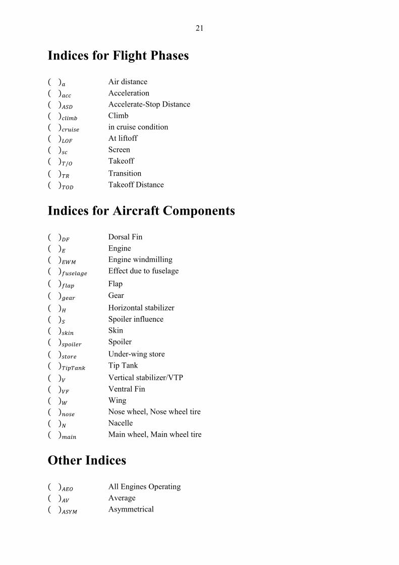
Indices for Flight Phases
( ) Air distance
( ) Acceleration
( ) Accelerate-Stop Distance
( ) Climb
( ) in cruise condition
( ) At liftoff
( ) Screen
( ) Takeoff
( ) Transition
( ) Takeoff Distance
Indices for Aircraft Components
( ) Dorsal Fin
( ) Engine
( ) Engine windmilling
( ) Effect due to fuselage
( ) Flap
( ) Gear
( ) Horizontal stabilizer
( ) Spoiler influence
( ) Skin
( ) Spoiler
( ) Under-wing store
( ) Tip Tank
( ) Vertical stabilizer/VTP
( ) Ventral Fin
( ) Wing
( ) Nose wheel, Nose wheel tire
( ) Nacelle
( ) Main wheel, Main wheel tire
Other Indices
( ) All Engines Operating
( ) Average
( ) Asymmetrical
Page 22
22
( ) Aquaplaning
( ) Climb
( ) Compressibility influence
( ) Correction
( ) Calibrated airspeed
( ) In degrees Celsius
( ) Displacement
( ) Dynamic
( ) Excess
( ) Exposed
( ) Friction
( ) Data from GJE EXTGFD-003
( ) Ground influence
( ) Horizontal
( ) Indicated Airspeed
( ) Induced
( ) Impingement
( ) Idle thrust
( ) In Kelvin
( ) From academic reference
( ) Load factor
( ) Maximum
( ) Minimum
( ) Minimum Control Ground
( ) Minimum Control Air
( ) Maximum Brake Energy
( ) One Engine Inoperative
( ) Profile
( ) Reflection
( ) Rudder
( ) Rotation
( ) Stall
( ) Half of the total value
( ) stopping
( ) True Airspeed
( ) Thrust factor
( ) Full Thrust
( ) total
( ) Wetted area
( ) In X-Direction of the aircraft
Page 23
23
List of Abbreviations AFM Airplane Flight Manual
AFMS Airplane Flight Manual Supplement
AMC Acceptable Mean of Compliance
AOA Angle of Attack
ASD Accelerate-Stop Distance
ASDA Accelerate-Stop Distance Available
BFL Balanced Field Length
BPR Bypass Ratio
CAS Calibrated Airspeed
CFD Computational Fluid Dynamics
CG Center of Gravity
EAS Equivalent Airspeed
EPR Engine Pressure Ratio
GFD Gesellschaft für Flugzieldarstellung
IAS Indicated Airspeed
ISA International Standard Atmosphere
ITT Interstage Turbine Temperature
KCAS Knots Calibrated Airspeed
KIAS Knots Indicated Airspeed
MAC Mean Aerodynamic Chord
MSL Mean Sea Level
NPA Notice of Proposed Amendments
NPRM Notices of Proposed Rule Making
OAT Outside Air Temperature
PA Pressure Altitude
PIC Pilot in Command
PNF Pilot Non Flying
QNH Barometric Pressure Adjusted to Sea Level
RPM Revolutions per Minute
RWY Runway
SL Sea Level
TAS True Airspeed
TOD Takeoff Distance
TODA Takeoff Distance Available
TOFL Takeoff Field Length
TOR Takeoff Run
TORA Takeoff Run Available
TOW Takeoff Weight
VTP Vertical Tailplane
ZFW Zero Fuel Weight
Page 24
24
1 Introduction
1.1 Motivation
The background of this project lies in the current certification status of the GFD fleet of Lear-
jet 35A/36A. Flight operation in the special configuration with under-wing stores installed is
currently only permitted for dry runway conditions.
In order to operate the aircraft with installed stores also in wet runway conditions, an adden-
dum is required that extends the operational envelope for takeoff on wet runways with under-
wing stores installed on the GFD fleet of Learjet 35A/36A. This report outlines the set-up of a
numerical takeoff performance simulation for this configuration. Because the results of this
report may be the basis of performance charts used in the daily flight operations, a focus has
been put on the very accurate determination and modeling of aircraft parameters and certifica-
tion requirements. This is also why a tendency to conservative approaches has been chosen in
cases where assumptions had to be taken.
No operational experience is available to give an indication on the order of magnitude of addi-
tional spray impingement drag due to under-wing stores installation. Therefore, this effect has
been a special area of investigation, since the certification requirements for wet and/or con-
taminated runways require the spray impingement drag to be considered, though without
providing specific equations to determine this fraction of the total precipitation drag.
Page 25
25
1.2 Definitions
Takeoff Distance (TOD)
According to CS-25.113, the Takeoff Distance (TOD) is the distance required for the aircraft
to reach an obstacle height above the runway surface measured from the brake release point.
The obstacle height to be cleared is 35 ft on a dry runway and 15 ft on a wet runway. The dis-
tinction between the All Engines Operative (AEO) and the One Engine Inoperative (OEI)
takeoff configuration is made. The configuration leading to the more conservative result be-
comes limiting.
Accelerate-Stop Distance (ASD)
In case of an aborted takeoff, CS-25.109 defines the Accelerate-Stop Distance (ASD) as the
overall ground distance that includes both the acceleration up to the speed at which the deci-
sion to abort the takeoff is made and the braking distance required to bring the aircraft to a
complete stop from this speed. Safety margins and pilot reaction times need to be considered.
Liftoff Distance
The Liftoff Distance is defined as the distance covered from the brake release point to the
point at which the aircraft first becomes airborne. The speed at which this distance is covered
is referred to as the Liftoff Speed, VLOF.
Balanced Field Length (BFL)
The Balanced Field Length (BFL) is the distance resulting from a critical engine failure at the
unique speed that leads to equal distances to either continue or abort the takeoff from this
speed. The TOD and the ASD are equal at the Balanced Field Length. The Balanced Field
Length therefore represents one possible limitation on the minimum runway length that needs
to be available for the aircraft taking off.
Decision Speed V1
The Decision Speed is the maximum speed to abort the takeoff and the minimum speed to
continue the takeoff when the runway length available equals the Balanced Field Length. It
therefore marks the critical engine failure recognition speed at which the any of the two deci-
sions to either continue or abort the takeoff would lead to the same overall distance, the Bal-
anced Field Length.
Page 26
26
Takeoff Field Length
The TOFL is the greater of the Balanced Field Length and 115% of the All-Engines-
Operative Takeoff Distance and determines the minimum field length that needs to be availa-
ble for takeoff.
Wet Runway
According to EU-OPS 1.480, a runway is to be considered wet, when the runway surface is
covered with precipitation of a depth of up to 3 mm, or when it is covered with precipitation
such that it causes the surface to appear reflective, without significant areas of standing water.
Contaminated Runway
According to EU-OPS 1.480, a runway is to be considered contaminated when more than
25% of the runway surface area within the required length is covered by precipitation of a
depth equivalent to 3 mm or more in water depth.
Indicated Airspeed (IAS)
The Indicated Airspeed is the speed value shown on the flight deck by the airspeed indicator.
It may be calibrated for aircraft specific errors to yield the calibrated airspeed (CAS).
Calibrated Airspeed (CAS)
The Calibrated Airspeed is the Indicated Airspeed corrected for the aircraft specific errors.
Without compressibility effects at high speeds, it is equal to the Equivalent Airspeed (EAS).
Equivalent Airspeed (EAS)
The Equivalent Airspeed is the speed at which the aircraft would have to fly at ISA, MSL
conditions when the dynamic pressure experienced by the aircraft in the actual flight condi-
tions was to equal the dynamic pressure at ISA, MSL.
True Airspeed (TAS)
The True Airspeed is the speed of the aircraft with respect to the surrounding mass of air.
Without wind influence, the True Airspeed equals the ground speed.
Critical Engine
According to CS-25 definitions, the critical engine is the one whose failure would most ad-
versely affect the performance or handling qualities of an aircraft.
Page 27
27
Bypass Ratio (BPR)
The Bypass Ratio is the ratio of the mass flow through the fan of a turbofan engine as com-
pared to the mass flow through the core of the engine.
Flat Rating
The term Flat Rating refers to the fact that the maximum deliverable thrust of an engine is
limited to a static maximum thrust rate for operation below a specific outside air temperature.
Hence, the engine thrust does not vary with temperature at outside air temperatures below the
flat rate temperature.
Precipitation Drag
Precipitation drag according to the EASA AMC-25.1591 refers to the drag force experienced
by an aircraft in wet or contaminated runway conditions. It consists of the displacement drag
of the tires through a water pool, the skin friction drag of water particles along the fuselage
and the spray impingement drag of water particles colliding with the exposed surfaces of the
aircraft.
1.3 Project Objectives
In terms of project objectives, there were three major fields of interest that are covered in this
report.
The first objective was to conduct a comprehensive investigation and determination of all rel-
evant aircraft parameters necessary for a detailed basic modeling of the aircraft. Only limited
aircraft performance data has been available, which is why the parameter determination was
done in a general approach applicable to any type of airplane. An overview on the parameters
required and applied either by certification or physical exigencies has been part of the analy-
sis. This permits to compare with other possible approaches the approach and assumptions
chosen for the performance simulation.
The second objective was to elaborate a simulation concept in a numerical computing envi-
ronment that permits to accurately model the aircraft performance during the takeoff with re-
gard to time- and speed dependant parameter variation. The numerical simulation method is
expected to offer a precision benefit over simplified approaches based on averaged parame-
ters. The numerical simulation shall be capable to deliver reliable charts for Balanced Field
Length and the Decision Speed V1 for a range of different airport environmental parameters.
Page 28
28
The third objective the report discusses is an analytical consideration of the spray impinge-
ment drag exerted on the aircraft fuselage by precipitation on the runway. Focus of this inves-
tigation was put on the large under-wing stores. The findings made and the approach chosen
can be of interest for other aircraft calculations.
1.4 Main Literature
Main assumptions and parameters for the report were taken from three major fields of refer-
ence data.
Since the results of the takeoff performance calculations shall be the baseline for actual air-
craft operations, one focus was put on the certification requirements governing takeoff per-
formance determination. The CS-25 and passages from EU-OPS 1 have been the basis for the
analysis, complemented by Acceptable Means of Compliance (AMC) applicable to certain
aspects of the discussed problems. This permitted to set up a basic simulation infrastructure
that could be fed with specific performance characteristics of the Learjet 35A/36A.
As only limited performance data of the Learjet 35A/36A in the specific operator’s configura-
tion is available, analytical approaches to determine aircraft performance parameters based
on geometry and other data available on the aircraft had to be investigated. Renowned litera-
ture from preliminary aircraft design was best suited for application in this purpose. Main
sources are the “Synthesis of Subsonic Airplane Design” by E. Torenbeek, as well as the vol-
ume “Airplane Design” by J. Roskam. Furthermore, “Aircraft Design – A conceptual ap-
proach” from D. P. Raymer was used mainly to obtain estimates from simple equations as a
means to validate the results obtained acc. to Roskam and Torenbeek. Also, “Fluid Dynamic
Drag” by S. F. Hoerner was a valuable source used for parts of the drag coefficient estimation.
Wet runway operations are one of the most dangerous operation scenarios for an aircraft.
Therefore, the effects of the wet runway conditions for the takeoff performance determination
were considered thoroughly. In addition to the certification documents, a number of re-
search papers investigating precipitation drag on a wet runway have therefore been analyzed.
Most notable in this respect is the work of NASA on “Measurements of Flow Rate and Tra-
jectory of Aircraft Tire-Generated Water Spray” as well as the ESDU document “Estimation
of spray patterns generated from the sides of aircraft tyres running in water or slush”. NLR
investigations of the latter documents in a CFD spray simulation and a comparison with flight
tested data has also proved to be of value for the analysis.
Also, three sources of aircraft performance data were used as a reference – the original AFM
of the Learjet 35A/36A, the AFMS 9702-2 Airplane Flight Manual Supplement as well as the
GJE EXTGFD-003 report.
Page 29
29
The GJE EXTGFD-003 report is the report that was used to create certified performance da-
ta for the aircraft with stores on a dry runway. It therefore serves as a good validation source
for the parameters determined on academic approaches.
The greatest challenge due to the complexity of the investigations was to select the approach
out of the many approaches proposed by the literature that was finally used in the perfor-
mance simulation for this report. The report therefore also serves to compare different ap-
proaches from the literature, if applicable.
1.5 Structure of the Report
The report is structured in eight main chapters that are arranged in a consecutive order.
Chapter 2 serves the reader to enter the topic of wet runway takeoff performance calcula-
tions. It is outlined which main factors have to be considered for the takeoff performance de-
termination specifically on wet runways, but also operational considerations are discussed.
Chapter 3 outlines the certification requirements and regulations that have been driving the
performance simulation development. The theory behind the various distance, reaction time
and speed definitions to be applied according to the certification documents is presented,
which is building the baseline for the subsequent calculations.
Chapter 4 contains all numerical relationships necessary to set up a numerical takeoff per-
formance simulation. It has been structured in a way that facilitates the distinction of the vari-
ous phases during the takeoff, in order for the reader to be able to trace the specific set of pa-
rameters that is employed in each of these phases. Numerical equations and estimation ap-
proaches are presented in this chapter, without referring to any specific aircraft. This permits
to neutrally describe model parameters without being influenced by specific characteristics,
and can therefore serve as the point of reference for the specific parameter discussion for the
Learjet 35A/36A performed in Chapter 6.
Chapter 5 outlines the investigation of additional drag force components due to the im-
pingement of water droplets on the aircraft surface performed for the Learjet 35A/36A. This
chapter takes into account a number of different research documents in order to analytically
determine the amount of drag caused by the specific Learjet 35A/36A geometry.
Chapter 6 is the point of convergence of all aircraft related parameter estimations developed
in Chapter 4 and shows the approaches selected from the literature in their application on the
specific aircraft.
Page 30
30
Chapter 7 presents the numerical takeoff performance simulation and gives an overview on
the functional architecture as well as the calibration concept employed. The simulation inte-
grates all relations outlined in the previous chapters of this report into a single program that
autonomously performs the takeoff performance simulation. The results obtained by this sim-
ulation are then validated, compared and analyzed in chapters 8, 9 and 10.
Chapter 8 therefore presents the simulation results obtained from the calculations. This in-
cludes a comparison of the results to known data and a simpler calculation method.
Chapter 9 is then used to outline possible error sources and influences on the takeoff perfor-
mance simulation. For that reason, a parameter variation analysis is presented that aims at val-
idating the behavior of the simulation with a change in the input parameters.
Chapters 10 and 11 bring the report to a conclusion with concluding remarks on the calcula-
tion and parameter estimation approach as well as recommendations for possible further im-
provements of the takeoff performance simulation.
Detailed analysis or validation that would leave the common thread of a chapter or section is
included in the Appendix of this report.
Page 31
31
2 Operational Hazards
2.1 Hazards from Wind, Rain, Snow and Ice
The takeoff phase is one of the most challenging and dangerous phases in the complete flight.
Many factors influence the safe conduct of a takeoff sequence. The presence of environmental
factors such as wind, rain, snow and ice is crucially impacting the performance of the aircraft
as compared to operation on a dry standard day.
Effect of Wind
The effect of wind on the performance determination is important to consider, as it can have a
different effect on the aircraft depending on its direction. The most favorable condition possi-
ble is the wind coming from the direction in which the aircraft is about to take off. This
headwind component will reduce the takeoff distance because the aircraft lifts off at a relative
air speed. A headwind component therefore requires less energy and acceleration distance
since a portion of the required liftoff speed is already imparted on the aircraft due to wind. In
contrast to this, an adverse effect will be seen when the wind comes from behind the aircraft
due to a reversal of the effect described above.
When the wind comes from a side angle (referred to as cross wind) to the runway, this will af-
fect the directional stability of the aircraft (especially in slick runway conditions) due to the
fact that a side force is acting on the aircraft as a whole, and a moment around the z axis is in-
duced through the rudder area which represents an disproportionally big partial area of the fu-
selage side view. This represents a hazard because of the risk to slide sideways off the runway
as well as through a yaw moment present as soon as ground contact is lost which leads to a
bank angle and might result in wing tip contact to the ground or destabilized takeoff. There-
fore, a maximum cross as well as tail wind speed needs to be predetermined.
Effect of Precipitation
Rain, snow and ice are having physical implications on the airplane itself as well as on the
runway surface conditions. The role of precipitation as runway contaminants is of high im-
portance for the takeoff distance and decision speed determination and is considered specifi-
cally in the upcoming sections. Snow and ice in this respect should be seen as to have the
same effect as rain, except for the greater magnitude of their impact. Icing on wings, engine
nacelles and control surfaces though is an effect does not occur in rain but poses a very con-
siderable threat that needs to be taken into account. Also, the damage to the aircraft due to
small stones contained in sputtered water or ice parts raised by the wheels being dashed
against the fuselage poses a further hazard to the aircraft (NLR-TP-2001-216).
Page 32
32
Even though jet engines are designed to ingest a certain amount of water while continuing to
operate normally, deteriorated and high intensity ground water spray is not beneficial for the
safe operation (risk of compressor stall, engine flame-out, and foreign object damage/FOD).
Therefore, the precipitation spray may not directly be pointed towards the engine intake
(EASA AMC E 790). Aircraft manufactures therefore foresee provisions to prevent the pre-
cipitation spray from being directed at sensitive areas. This consideration will be of im-
portance in the later determination of the actual spray geometry of the Learjet 35A/36A.
Another factor to consider is the reduced visibility in adverse weather conditions, possibly in-
creased by waft-back water or snow particles due to thrust reversing (NLR-TP-2001-204).
2.2 Definitions for Wet and Contaminated Runways
The calculations performed by means of the methods described in this report shall be done for
wet runway conditions. This term needs to be differentiated from the term contaminated run-
way conditions.
The margin for standing water depth on the runway for the classification as a wet runway is 3
mm, beyond which the runway is to be considered contaminated. It is to be always considered
contaminated when covered with snow, slush or ice.
EU-OPS 1.480
A runway is considered wet when the runway surface is covered
with water or equivalent, [with a depth less than or equal to 3 mm], or when there is a
sufficient moisture on the runway surface to cause it to appear reflective, but without
significant areas of standing water.”
(…)
A runway is considered to be contaminated when more than 25% of the runway surface area
(whether in isolated areas or not) within the required length and width being used, is covered by –
(a) surface water more than 1/8th inch (3mm) deep
(…)
According to EU-OPS 1.475 (d), a wet runway may, as long as it refers to a concrete/asphalt
covered runway, also be considered as dry in terms of performance parameters. However, a
damp runway is closer to a wet runway in terms of braking action, which therefore must spe-
cifically be addressed in a wet runway condition. However, no precipitation effects other than
the braking coefficient degradation are determined in the Certification Specification CS-
25.109.
Page 33
33
Normative literature or regulations such as EASA AMC 25.1591 exists specifically for con-
taminated runway conditions. The latter does include specific equations that can be used in
order to approximate specific physical precipitation effects upon the airplane. They will be
discussed in detail in the performance parameters discussion.
2.3 Wet Runway Effects on Aircraft Performance
The performance on wet runways changes in some crucial factors for the operation of the air-
craft. There are three major impacts on the aircraft performance that result from an operation
on a wet runway:
additional drag induced through the fluid-aircraft interaction
reduced braking force due to significantly decreased braking coefficient
Aquaplaning/Hydroplaning
These will be discussed in detail in the following sections.
2.3.1 Aquaplaning
According to NASA-TN-D-2056, aquaplaning occurs on smooth runways at a fluid depth of
2mm and more. For a wet runway with fluid depths of up to 3mm, it is therefore relevant to
consider aquaplaning.
The aquaplaning speed is determined from EASA AMC 25.1591 Section 7.1.1as
√
(1.1)
With
Tire pressure in lb/in²
Aircraft aquaplaning ground speed in kts
Aquaplaning has three major effects that are of importance and have to be considered in the
calculations.
Since the tire begins to float up, it subsequently loses contact to the runway surface (tarmac)
and directional control through wheel to ground contact is considerably reduced.
Page 34
34
This is of importance if the aircraft minimum control speed of the aircraft2on ground, VMCG, is
close to or even higher than the aquaplaning speed of the aircraft because then directional
control of the aircraft is very limited.
Likewise, braking forces, applied in case of an aborted takeoff, are reduced due to the flota-
tion of the tire.
A third factor of aquaplaning is the reduction of drag due to aquaplaning. As the tire starts to
float, it displaces less water, which leads to a decrease in the displacement drag force. EASA
AMC 25.1591 provides an estimation for the effect of the drag reduction due to aquaplaning
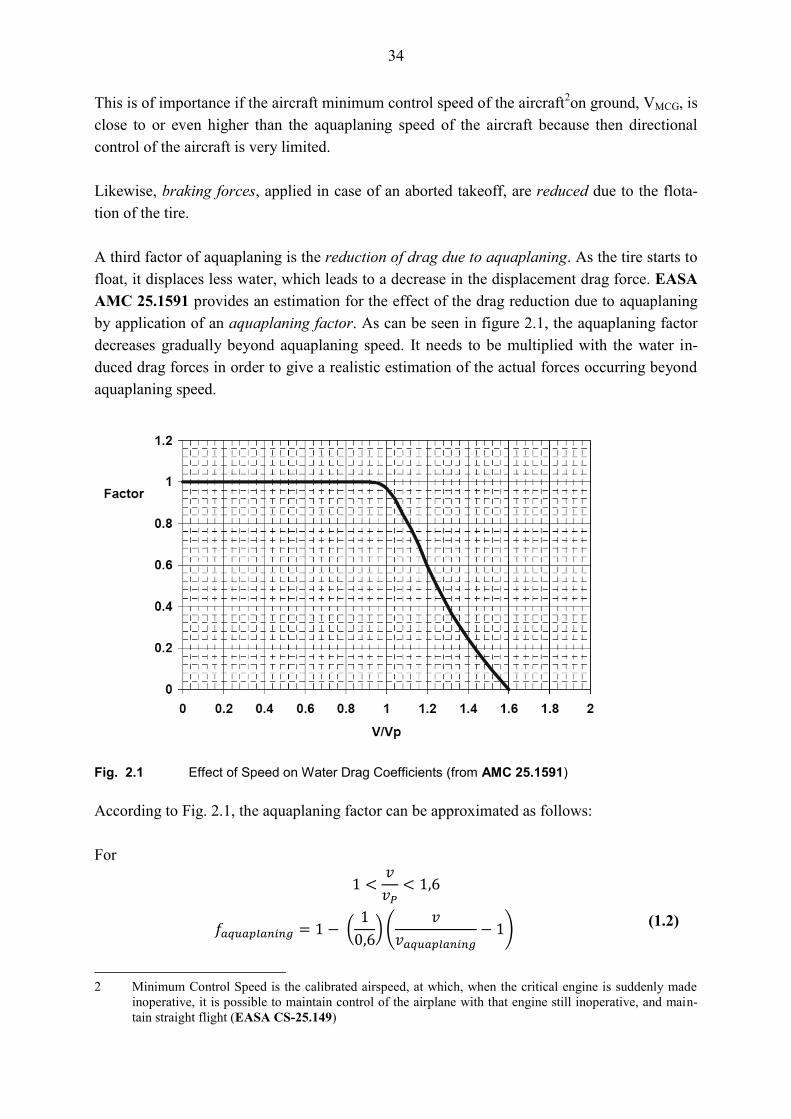
by application of an aquaplaning factor. As can be seen in figure 2.1, the aquaplaning factor
decreases gradually beyond aquaplaning speed. It needs to be multiplied with the water in-
duced drag forces in order to give a realistic estimation of the actual forces occurring beyond
aquaplaning speed.
Fig. 2.1 Effect of Speed on Water Drag Coefficients (from AMC 25.1591)
According to Fig. 2.1, the aquaplaning factor can be approximated as follows:
For
(
) (
)
(1.2)
2 Minimum Control Speed is the calibrated airspeed, at which, when the critical engine is suddenly made
inoperative, it is possible to maintain control of the airplane with that engine still inoperative, and main-
tain straight flight (EASA CS-25.149)
Page 35
35
With
Aquaplaning Factor
Aircraft Ground Speed
Aircraft aquaplaning ground speed
2.3.2 Acceleration
The acceleration capability of the aircraft is impacted by the wet runway conditions by nu-
merous factors. NLR-TP-2001-204 and the AMC 25.1591 outline 3 major precipitation drag
components for Aircraft operation on wet runways which are also referred to as precipitation
drag forces:
Displacement Drag (Tires)
Impingement/Collision Drag (direct collision on aircraft components)
Skin Friction Drag
Also, the tire-to-ground rolling friction on a wet runway is impacted by the wet runway condi-
tion. The detailed equations for this component will be discussed in Section 4.1.9.
Fig. 2.2 Precipitation Drag Forces due to Contaminated Runway Conditions
All these force components impact the acceleration capabilities of the aircraft negatively and
represent a drastic difference to a dry runway operation. According to NLR-TP-2001-204,
they are also subject to piloting technique, because the pilot can reduce or increase the amount
of drag by slight unloading/loading of the front wheel of the aircraft through elevator input
during the ground roll. If applied correctly, this technique can reduce the precipitation drag
during the acceleration, or increase the drag during the deceleration of the aircraft, as desired
by the applicant.
Page 36
36
Displacement Drag
The displacement drag is the drag force which results from the wheel contact to the runway
surface. Below aquaplaning speed, the wheel is creating a “dry spot” at its runway-tire contact
surface. Therefore, it has to displace the amount of water that was previously at this now dry
spot which creates a drag force. The faster the tire moves, the more energy is incurred in the
water bow wave that forms, until the surface tension of the water is overridden and a spray
pattern emerges. This spray itself then creates new forms of precipitation drag which are spray
collision (impingement) and skin friction drag.
Impingement Drag
As soon as the tire induced water wave emerges from the puddle, droplets may impinge on the
aircraft components. Unfortunately, the EASA AMC 25.1591 does not provide quantifiable
information to determine the magnitude of this impingement drag force. Therefore, as part of
the investigative objectives of this work, a special section is introduced to determine the actu-
al amount of collision drag especially due to the installation of under-wing stores but also on
other exposed surfaces of the airframe. The calculation of this retarding force requires to be
considered in dependence of speed, due to the fact that the collision impulse magnitude of wa-
ter droplets is speed-dependant. The drag reduction factor due to aquaplaning also needs to be
considered.
Skin Friction Drag
The skin friction drag that is mainly caused by the water spray from the front wheel is conser-
vatively considered through the simple equation provided in Section 7.1.3 b.2 of EASA AMC
25.1591. This equation determines a drag coefficient from the length of the wetted fuselage.
The wetted fuselage is assumed to amount for 75% of the total length of the fuselage, since
the top of the spray plume is expected to reach the fuselage behind the front wheel. The drag
reduction factor due to aquaplaning needs to be considered.
Rolling Friction
The rolling friction on a wet runway is higher than the rolling friction on a dry runway. The
determination of the friction force is requires the aircraft lift force as an input, because the
weight of the aircraft and the lift force together determine the normal force acting on the
wheels. This normal force then determines the retarding force component when multiplied
with the rolling friction coefficient for a wet runway.
Page 37
37
2.3.3 Deceleration
Deceleration is part of the takeoff performance calculation, because an aborted takeoff due to
malfunction necessitates the aircraft to be brought to a halt on the runway. While the retarding
forces described above will be maintained and assist the deceleration of the aircraft, a wet
runway still has a negative impact on the deceleration capabilities of an aircraft. This is be-
cause the effect of higher drag forces is overridden by a major decrease in braking friction
that results from an increased sleekness of the runway.
Braking coefficients for dry runways can best be obtained from flight test data. Clearly, the
braking coefficient for a wet runway can never be higher than that for a dry runway.
This is confirmed by the relationship given in Fig. 2.3 which relates wet runway surface fric-
tion to the dry runway surface friction coefficient for grooved and smooth runway surfaces.
Fig. 2.3 Available Traction at Tire-Surface Interface (NASA TM-X-72650)
Page 38
38
As can be seen clearly, the overall friction coefficient and hence the braking capability of the
aircraft wet runway is roughly half that of the aircraft on a dry runway.
The reduced deceleration performance of the aircraft and the reduced acceleration perfor-
mance of the aircraft combined result in higher Accelerate-Stop Distances for aborted takeoff
runs. Since one major retardation device are the aircraft brakes, the speed at which a flight can
safely be aborted and from which an aircraft can be brought to a complete stop on a runway of
specific length will always be lower in wet condition as compared to dry conditions.
2.3.4 Directional Stability
The directional stability of the aircraft refers to its movement along the runway center line.
Since the simulation as one of the project objectives outlined at the beginning of the report is
being developed for a longitudinal motion, the directional stability determination is beyond
the scope of this report. However, it is still an aspect influenced by the wet runway condi-
tions, so it shall be briefly discussed.
The major force that is playing a role in terms of directional stability on wet runways is the
sideways acting friction force of the tire. Similar to the linear motion friction, this force is be-
ing reduced by the adverse runway surface conditions. The aircraft can sustain less side
force/momentum on slick surfaces, which is of relevance when the pilot is required to exert
such a force in order to keep the aircraft on the runway center line during the takeoff run.
This effect is worsened by all factors that influence the momentum around the yaw-axis of the
aircraft, such as the loss of an engine (differential thrust), side wind but also aileron deflection
that might decrease the normal load on the critical tire and thus further reduce its sideway
friction force. The effect is also worsened by uneven distribution of the surface contaminant,
such as water or ice patches causing a braking action imbalance which may lead to the aircraft
veering off the runway.
Page 39
39
2.4 Responsibilities, Precautions and Airmanship
From a pilot’s point of view, the variety of factors effecting aircraft performance and handling
qualities plays a role in his overall flight condition assessment and the subsequent briefing. As
part of the flight preparation, all of these factors need to be considered.
According to EU-OPS 1.490 sections a) and b), the operator being the responsible pilot in
command (PIC) has to consider the maximum takeoff mass and the takeoff distances/V1 be-
fore taking off in his current configuration. The fact that these performance data are currently
not available for the Learjet 35A/36A discussed in this report with under-wing stores installed
in wet runway conditions motivates the investigations and calculations presented in this re-
port.
When determining the maximum takeoff mass, the operator/pilot has to take account for
headwind component, runway alignment distance, pressure altitude at aerodrome, ambient
temperature at aerodrome, runway slope as well as runway surface type and condition. It is
necessary for the flight crew to be prepared for a rejected takeoff during the takeoff roll,
therefore the briefing needs to address specifically the rejected takeoff case and the speed up
to which such an abort is still safe. The decision of whether to stop or to go is taken by the
PIC, because this decision action has a significant impact on the flight safety. The PIC will
therefore keep the hands on the thrust levers until the aircraft reaches the speed V1, even when
he is the pilot non-flying (PNF). If a malfunction or problem occurs during the takeoff roll,
the captain will call out his decision to confirm whether the takeoff run will be continued or
aborted3.
Therefore, the appropriate performance charts representing the present conditions or a correc-
tion factor to be applied to values for standard conditions are to be used in the flight prepara-
tion. These are contained in the AFM or the AFMS. Because the aerodynamic qualities of the
aircraft (influencing Vs, VMCG, VR, VMCA, V2) do not change for wet runway operations, none
of the aerodynamically derived aircraft speeds changes. Only V1 is impacted by the degraded
runway conditions, as discussed in Section 2.3.3.
3 The procedures described here are the standard procedures acc. toFAA AC 120-62. They can, however,
vary depending on the operator specific AFM procedures given for the respective flight crews.
Page 40
40
3 Certification Regulations
3.1 Overview of Regulations for the Takeoff
As for any other part of aviation, many regulatory requirements and definitions have been
made to describe the takeoff phase of the aircraft. Those that are relevant to the determination
of the takeoff distance and the abort speed shall be outlined in this paragraph.
The jet aircraft takeoff performance is being addressed in the Part 25 of both the Federal Avi-
ation Regulations (FAR) of the FAA (Federal Aviation Authority, USA) and in their equiva-
lent, the Certification Specifications CS-25 (former JAR-25) issued by the EASA (European
Aviation Safety Agency) in Europe. As the regulations of EASA and FAA contents are al-
most similar to each other, the EASA CS-25 shall be the reference for further argumentations
used in this report.
Generally, the relevant CS-25 sections are specifying the details to be available to the operator
in terms of aircraft performance information, the takeoff speeds, takeoff trajectory, as well as
providing definitions for the limiting takeoff distances necessary in two cases.
The distinction is made between the Accelerate-Go (Takeoff) and the Accelerate-Stop (Abort-
ed Takeoff) Case. The respective distances are the Takeoff Distance (TOD) and the Acceler-
ate-Stop Distance (ASD). Both of these cases distinguish again between an attempted takeoff
with All Engines Operating (AEO) and with One Engine Inoperative (OEI), the less favora-
ble, longer distance in either condition becomes limiting. In addition, there is other regulatory
material complementing the CS-25 for certain detailed aspects of the takeoff performance cal-
culations.
The regulation Section CS-25.105 specifies the general takeoff data that needs to be available
to execute a takeoff. It requires that takeoff speeds, distances and the takeoff path be deter-
mined for a selected aircraft configuration and runway condition as a function of weight, alti-
tude and ambient temperature. Subsequently, the definitions for these requirements are given
in the relevant sections of CS-25 listed below.
The takeoff speeds are defined in section CS-25.107, listing the definitions for VEF, the criti-
cal engine failure speed, V1, VMU, VR, VLOF, V2 and VFTO. All speeds except for VEF and V1
are determined from aerodynamic performance data of an aircraft.
Page 41
41
When these aerodynamically derived speeds are already known for an aircraft configuration,
the speed V1 and its associated VEF are therefore the only unknown parameters that need to be
determined with the new environmental conditions and effects outlined in Chapter 2. This is
the case for the calculation performed in this report for the Learjet 35A/36A, and the V1 speed
is derived from the Balanced Field Length Calculation discussed in Section 3.6.
The distance covered during an aborted takeoff is the Accelerate-Stop Distance (ASD), whose
definition is regulated by Section CS-25.109. It is applied for the case that the decision to
abort the takeoff run occurs before or at the takeoff decision speed V1. Both the AEO and the
OEI conditions are to be considered to determine the limiting condition. CS-25.109also speci-
fies basic braking friction values for wet runways as a function of tire pressure. These values
may be used if no more detailed test data for the specific aircraft are available.
The takeoff path is regulated in Section CS-25.111 and specifies the procedure from the point
at which the standing aircraft initiates the takeoff until transition to en-route configuration or a
point 1500 feet above ground and considers the case of an engine failure at VEF. It is of high
relevance for the takeoff calculations performed in this report, as it specifies the takeoff path
and procedure the aircraft needs to be able to follow when an engine failure occurs after V1. It
equally specifies minimum climb gradients during the takeoff path, which will play a role in
the validation of the final calculation results at the end of this report.
Section CS-25.113 defines the takeoff distance and the takeoff run. It differentiates the AEO
and the OEI conditions. For the OEI condition, a takeoff with assumed engine failure in ac-
cordance to CS-25.111 needs to be considered. For the AEO condition, a safety factor of 1,15
needs to be applied to the takeoff distance. The higher resulting distance from both methods
becomes limiting. Both conditions have been considered in this report.
Both takeoff and landing are the maneuvers associated with the highest risk during the flight.
In the history of the FAR/CS-25, many amendments have therefore been made to the original
certification requirements in order to account for lessons learned from previous incidents and
to improve the overall safety of aviation. These Amendments are proposed through JAA No-
tice for Proposed Amendments (NPA) and/or FAA Notices of Proposed Rule Making (NPRM)
and then introduced as FAR or CS Amendments. Of importance for this report is especially
the FAR Amendment 25-92 which includes the requirement to include specific considera-
tions for wet runway conditions in the takeoff performance calculations. Notable for this re-
port are also the FAR Amendment 25-42 in combination with the EASA AMC 25.101(h)(3)
with respect to the different pilot recognition and reaction times to be considered in the Ac-
celerate-Stop Distance calculation.
Page 42
42
In order to assist the practical application of the regulatory Certification Specifications (CS),
the EASA also issues Acceptable Means of Compliance (AMC) documents. These AMC pro-
vide qualified technical interpretative material that may, but does not have to be used, in order
to comply with certification requirements set by the CS. Acceptable Means of Compliance
documents have therefore been used in this report. The most important document used is the
EASA AMC 25.1591, which specifies equations and calculation approaches to assess the
takeoff performance on contaminated runways.
Due to the nature of frequently updated regulations, it is of importance to make a judgment on
the applicability of certain regulatory requirements when developing supplementary certifia-
ble calculations or design for a specific aircraft. Due to a “grandfathering clause”4 it can, but
does not have to be the most current version of the regulatory requirements that is applicable
to the existing aircraft.
3.2 Aircraft Speeds during Takeoff
For the aircraft, characteristic speeds are denominated with a capital V entailed by a subscript,
they are referred to as V-Speeds. V-Speeds are provided to the operator in Indicated Air
Speed (IAS) or Calibrated Air Speed (CAS), according to the speed displayed on his speed
indicator. During the takeoff roll in normal, AEO conditions, there are four major V-Speeds
that need to be considered for the performance calculation. These are the Takeoff Decision
Speed V1, the Rotation Speed VR, the Liftoff Speed VLOF and the safe climb speed V2. In OEI
conditions, the speed at which the engine fails, VEF, is another very important parameter. V1 is
the highest speed at which a takeoff can still safely be aborted and represents one of the most
important speeds in the takeoff performance determination.
There are a number of other relevant V-Speeds which are acting as limitations due to aerody-
namic or mechanic properties of the aircraft. In fig: 3.1, they are indicated with a red band for
the mechanical and with a blue band for the aerodynamically limiting speed regions.
4 This refers to the fact that older aircraft may still be certified under older regulatory requirements if the
original aircraft has been certified according to older standards applicable at the time of initial certifica-
tion.
Page 43
43
Fig. 3.1 Takeoff Speeds and ground distances in AEO condition (Airbus 2002)
From a mechanical point of view, one limiting speed is the maximum tire speed VTIRE, justi-
fied from the maximum centrifugal forces on the aircraft tires. Another limitation is the Max-
imum Brake Energy Speed VMBE. This is the takeoff mass dependent maximum speed up to
which the aircraft brakes are able to dissipate the kinetic energy of the airplane in a stopping
case. If the aircraft is faster and has kinetic energy higher than the maximum brake energy
limit, the aircraft braking system cannot sustain sufficient braking action to bring the aircraft
to a complete stop. As a consequence, the highest speed at which a takeoff could be aborted is
VMBE, an upper boundary for V1. CS-25.109 specifies that a flight test demonstration of the
maximum brake kinetic energy accelerate-stop distance must be conducted with no more than
10% of the allowable brake wear range remaining on each of the wheel brakes.
Aerodynamically justified characteristic V-Speeds have to be flight-tested, they will be found
in the AFM of a certified aircraft. They can be approximated as a function of the stall speed of
the aircraft at 1g vertical acceleration, VS,1g or VS. The estimation for VLOF is presented ac-
cording to Roskam VII, the VR and V2 estimations according to GJE EXTGFD-003.
(3.1)
(3.2)
(3.3)
Page 44
44
Also, the minimum control speeds have to be determined in flight test. CS-25.149 specifies
the VMC as follows:
VMC is the calibrated airspeed, at which, when the critical engine is suddenly made
inoperative, it is possible to maintain control of the aeroplane with that engine still inoperative,
and maintain straight flight with an angle of bank of not more than 5º.
The stability properties of the aircraft and the means to stabilize the aircraft on the ground are
different to those in the air; therefore there is a distinction between VMCG (ground) and VMCA
(air). Due to this stability criterion, the rotation speed VR can never be lower than VMCA.
Likewise, the decision speed V1 can never be lower than VMCG. The aircraft in an OEI condi-
tion would not be able to sustain stable conditions. This is of importance for the takeoff per-
formance calculation when the V1 and VR speeds coincide with the VMC requirements, usually
for low takeoff masses.
The Minimum Unstick Speed VMU shown in Fig. 3.1 is the lowest speed at which the aircraft
can get airborne. However, due to the large Angle of Attack (AOA) necessary, the lift-to-drag
ratio is unfavorable and not optimal to clear the obstacle height at minimum distance.
The following procedure describes a takeoff in AEO conditions as shown in Fig. 3.1. The
aircraft will accelerate from the brake release point passing the Takeoff Decision Speed V1
towards the rotation speed VR. The nose of the aircraft is rotated (about 3°/s5) and the aircraft
lifts off at liftoff attitude at the speed VLOF and climbs out accelerated. The objective is to pass
an obstacle at a specific height at the end of the runway at the safe climb speed V2. In case of
a wet runway, when the required obstacle clearance height is reduced to give a performance
benefit, the V2 can still be reached at the original obstacle clearance height defined for dry
runways.
In OEI conditions, an engine is assumed to fail at a specific speed VEF as defined in CS-
25.107. Should this critical malfunction occur before the decision speed V1, the pilot will take
action to abort the takeoff run. Should the engine fail after passing V1, the pilot will not abort
the takeoff run because the remaining stopping distance would not be sufficient, and continue
the takeoff under OEI conditions.
The following definition from CS-25.107 serves as a baseline for the further discussions and
calculations of the OEI condition in this report. It marks the difference between VEF and V1.
(a)(2) V1, in terms of calibrated airspeed, is selected by the applicant; however, V1
may not be less than VEF plus the speed gained with the critical engine inoperative
during the time interval between the instant at which the critical engine is failed, and
the instant at which the pilot recognises and reacts to the engine failure, as indicated
by the pilot's initiation of the first action (e.g. applying brakes, reducing thrust,
deploying speed brakes) to stop the aeroplane during accelerate-stop tests.
5 this pitch rate is a common orientation but may vary for specific aircraft and/or configurations
Page 45
45
The most critical VEF is so close before V1 that the engine failure recognition occurs exactly at
V1. This is the most critical and highest speed, because at V1 both GO or STOP decisions co-
incide and the aircraft will either have to accelerate with OEI from this lowest speed to pro-
ceed with a takeoff, or brake from this maximum reject speed down to a full stop. V1therefore
defines the boundary between the GO and the STOP case and its knowledge therefore is of
major importance in the takeoff preparations and will be determined in this report. In contrast
to the other speeds discussed, it is also dependent of the runway length available.
3.3 Distances in the Takeoff (Accelerate-Go) Case
The takeoff procedure of an aircraft can be divided into three major phases. The ground ac-
celeration phase, the rotation phase and the airborne acceleration phase together constitute the
Takeoff Distance (TOD). During the acceleration from brake release point to the point at
which VLOF is reached and runway contact is lost, the corresponding Liftoff Distance is cov-
ered. After liftoff during climb-out to screen height, the Air Distance is covered. The Liftoff
Distance also includes the Rotation Distance between the rotation point at VR and the liftoff
point. At the rotation point, the nose gear of the aircraft is raised from the runway to liftoff
AOA, while contact to the runway surface is sustained by the main gear.
Due to the requirement that a critical failure during the takeoff phase always has to be consid-
ered as discussed in Section 3.1, the AEO and the OEI conditions have to be calculated indi-
vidually to determine the limiting total TOD. When determining the takeoff performance in
an OEI condition, the ‘critical engine’ needs to be assumed to fail, which the CS-25 specifies
as the one that would most adversely affect the performance or handling qualities of an air-
craft.
Fig. 3.2 gives an overview on the discussed takeoff sequence for a takeoff in OEI conditions.
TOGA is the takeoff/go-around thrust, while N is the number of engines. This subscript is
used to distinguish the AEO (N) and OEI (N-1) conditions.
Page 46
46
Fig. 3.2 Takeoff in OEI Conditions (Airbus 2002)
The most important change between the certification requirements of the TOD of a wet run-
way compared to a dry runway is the reduction of the screen height from 35 ft to 15 ft as can
be seen in Fig. 3.2. This screen height is an assumed obstacle which the aircraft has to be able
to clear at the end of the Air Distance. CS-25.113 defines the Takeoff Distance as follows:
a) The takeoff distance on a dry runway is the greater of the following values:
TOD OEI dry as the Distance covered from the brake release to a point at which
the aircraft is 35 feet above the takeoff surface, assuming the failure
of the critical engine at VEF and recognition at V1,
1.15 factored TOD AEO dry equals 115% of the distance covered from brake release to a
point at which the aircraft is 35 feet above the takeoff surface,
assuming all engines operating.
b) The takeoff distance on a wet runway is the greater of the following values:
The take-off distance on a dry runway determined in accordance withCS-25.113 a)
TOD OEI wet as the Distance covered from brake release to a point at which the
aircraft is at 15 feet above the takeoff surface, ensuring the V2 speed to
be achieved before the airplane is 35 feet above the takeoff surface,
assuming failure of the critical engine at VEF and recognition at V1.
According to the above statement, the TOD on a dry runway, according to CS-25.113 b), can
also become limiting for the wet runway TOD. This seemingly redundant distinction is rele-
vant for aircraft that have a Thrust-to-Weight ratio so high that the reduced screen height of a
wet runway would lead to a smaller TOD than was needed on a dry runway.
Page 47
47
In the TOD calculation, the Air Distance does not necessarily have to be covered above the
actual runway surface. It can also be covered above a clearway, referring to a surface that
does not count as a part of the actual runway length, but is suitably shaped to allow the air-
craft to climb out to screen height, e.g. a grassy area at the end of the runway. It is beneficial
to consider the existence of a clearway, because it implies a performance benefit in the deter-
mination of the runway length required for takeoff.
In the case that a clearway is present, it is therefore necessary to distinguish between Takeoff
Distance and Takeoff Run (TOR). The TOR is related to the actual runway length that is used
for the acceleration to liftoff speed and may be smaller as the TOD because it takes into ac-
count the existence of a clearway to cover the Air Distance, as shown in Fig. 3.3.
Fig. 3.3 Takeoff Run and Takeoff Distance with Clearway considered (FAA AC 25-7B)
For a runway with clearway, CS 25.113 defines the Takeoff Run as follows:
a) The takeoff run on a dry runway is the greater of the following values
TOR OEI dry as the Distance covered from brake release to a point equidistant
between the point at which VLOF is reached and the point at which the
aircraft is 35 feet above the takeoff surface, assuming failure of the
critical engine at VEF and its recognition at V1,
115% of the TOR AEO dry as the distance covered from brake release to a
point equidistant between the point at which VLOF is reached and the
point at which the aircraft is 35 feet above the takeoff surface, assuming
all engines operating.
b) The takeoff run on a wet runway is the greater of the following values:
TOR OEI wet as the Distance covered from the brake release to a point at
which the aircraft is at 15ft above the takeoff surface, ensuring the V2
speed to be achieved before the airplane is 35 feet above the takeoff
surface, assuming the failure of the critical engine at VEF and
its recognition at V1.
115% of the TOR AEO wet as the distance covered from brake release to a
point equidistant between the point at which VLOF is reached and the
point at which the aircraft is 35 feet above the takeoff surface, assuming
all engines operating.
Page 48
48
According to CS-25.113, the TOD equals the TOR when no clearway is present. Without a
clear- or stopway available, a Balanced Field Length (BFL) can be determined. Consequently,
when a Balanced Field Length shall be determined such as in this report, the Takeoff Run
does not have to be considered separately and all relevant distances must be covered on or
above the runway surface.
For the purpose of flight planning, the pilot must match the Takeoff Distance (TOD) with the
Takeoff Distance Available at the airport (TODA), respectively the Takeoff Run (TOR) with
the Takeoff Run Available (TORA) when a clearway shall and may be considered. The Ac-
celerate Stop Distance Available (ASDA) is relevant for a rejected takeoff and is discussed in
Section 3.4. Fig. 3.4 shows a graphical representation of the relationships.
Fig. 3.4 TORA, ASDA and TODA with Clear- and Stopway available (Airbus 2002)
Page 49
49
3.4 Distances in the Accelerate-Stop Case
As opposed to the continuation of the takeoff after a critical failure such as the loss of an en-
gine, the pilot may also opt to bring the aircraft to a complete stop at or before V1 is reached.
Instead of further accelerating the aircraft, the pilot applies all available means of braking.
The overall ground distance that includes both the acceleration and the braking distance is
then referred to as the Accelerate Stop Distance (ASD).
Summarized according to CS-25.109, the ASD is defined as the sum of the distances to:
Accelerate the airplane with all engines operating to VEVENT,
Accelerate from VEVENT to V1 assuming the event motivating the rejection of the takeoff
occurs at VEVENT and the pilot takes the first action to reject the takeoff at V1
Come to a full stop
Plus a safety margin distance equivalent to 2 seconds at constant V1 speed
According to CS-25.109, the distinction between the AEO and the OEI case needs to be
made, the larger resulting Accelerate-Stop Distance of which condition becomes limiting. In
the OEI case, the trigger event is the engine failure occurring at VEF, and the aircraft is
brought to a stop with one inoperative engine. In the AEO case, the takeoff is rejected due to
an event which did not lead to the loss of an engine. Usually, the ASD under AEO conditions
is larger than under OEI conditions, as the failed engine produces a drag increment facilitating
the deceleration.
Fig. 3.5 Aborted Takeoff with Critical Engine Failure (Airbus 2002)
Page 50
50
If a stopway is available, in equivalence to the clearway philosophy this field may be used as
a performance benefit. The pilot may account for it in the Accelerate-Stop-Distance Available
(ASDA) when he compares this to the ASD for his operating conditions.
On wet runways, the reduced braking capacity needs to be taken into account for. CS-25.109
provides special braking friction coefficients for different surface and operating conditions for
wet runways.
3.5 Reaction Times after Critical Failure
When an engine of the aircraft fails or another event necessitates a rejected takeoff, the pilots
are required to react in a specified way in order to maintain control. The human reaction times
to activate the braking devices need to be taken into account for in the ASD by adding the dis-
tance equivalent to two seconds at V1 to the ASD. For a more detailed determination of these
reaction times, AMC 25.101 (h)(3) specifies the time steps to be considered between the acti-
vation of the retarding devices, while the two second distance shall be seen as a safety margin
to account for operational variability in the activation of braking devices.
As in the course of the report, a time-step based calculation method for the takeoff distances
will be shown, taking the detailed application sequence of braking devices into account is
possible. However, in the pace of historical development the CS/FAR-25 specification, there
have been a number of amendments with differing time step definitions. It is important to de-
termine if the original regulations valid at the time of first flight of the aircraft are to be taken
into consideration (grandfathering clause), or if the current regulatory basis should be applied.
According to Airbus 2002, the history of Amendments can be roughly divided into three
phases: before, within and after the CS/FAR Amendment 25-42 from March 1, 1978. The pre-
Amendment 25-42 CS/FAR 25 valid at first flight of the Learjet 35A/36A required no reac-
tion time distance to be added to the ASD. The CS/FAR Amendment 25-42 then required two
seconds of continued acceleration after V1 to add to the ASD. This was considered to be too
strict and the NPA 244 and NPRM 93-08 were incorporated into the CS-25.109 in 2000/1998.
This current version of the CS-25.109 requires adding two seconds at V1 speed to the total
distance instead of considering a continued acceleration. In turn it requires that the runway
surface condition is taken into account for (dry/wet), and specifies specific brake energy test-
ing requirements.
Page 51
51
For the deployment of braking means, FAA Advisory Circular AC 2025-7 (Chapter 2, section
2) specifies that the time delay between the activation of the second and third braking devices
is to be amounted for with one second each. This complies to AMC-25.101 (h)(3) which
states that the activation time delays must be validated with the operator and the demonstrated
time delays must be expanded as shown in Fig. 3.6.
Fig. 3.6 V1 and VEF Interdependence and Time Delay for Retardation Device Activation (AMC-
25.101 (h)(3))
In the case of the Learjet 35A/36A, applying the grandfathering clause in order to not consid-
er the two seconds reaction time distance in the ASD would not be conservative. It would also
require additional certification effort for the operator, because according to Airbus 1998 the
authorization to operate under the grandfathering clause must be obtained by the operator and
cannot be applied to an aircraft automatically.
Hence, for the calculations performed for the ASD in this report, the reaction times according
to Fig. 3.6 and AMC-25.101 (h)(3) are used, considering specific reaction times and a 2-
second equivalent distance margin at constant V1 speed.
Page 52
52
3.6 Balanced Field Length
As was pointed out in the previous sections, the decision speed V1 plays an important role in
the takeoff performance calculations. It requires considering the Takeoff as well as the Accel-
erate-Stop cases and their respective TOD and ASD. There is one single V1, at which reject-
ing the takeoff would lead to the same required distance as a continued takeoff. Rejecting the
takeoff after passing V1 would lead to a longer stopping distance and overall ASD than if the
takeoff was continued. The opposite is true for the TOD. Hence, the Balanced Field Length
(BFL) is the distance at which the TOD and the ASD are equal, as shown in Fig. 3.7. The
BFL therefore also represents a limitation to the minimum runway length that needs to be
available for the aircraft taking off, when no clear- or stopways are taken into account for.
Fig. 3.7 Balanced Field length as Equal Distance of ASD and TOD (Airbus 2002)
Considering a fixed takeoff-weight while varying the speed at which an engine is assumed to
fail, the following observations can be made for the TOD/ASD calculations:
If the assumed engine failure speed is increased gradually, the TOD required shrinks, since
the acceleration phase with all engines operating is longer. The same screen height at the end
of the airborne phase can be reached at a shorter overall distance.
At the same time, increasing VEF also increases the ASD, since both the distances due to the
reaction time delay as well as the total deceleration distance are becoming larger since more
kinetic energy is to be decelerated.
This means that the resulting distances TOD and ASD are essentially a function of VEF. If the
assumed engine failure speed is increased incrementally for the ASD and the TOD calculation
in the OEI case, two converging graphs are resulting.
Page 53
53
They are forming an intersection point at the BFL and the associated balanced V1. Figure 3.8
provides an example that was actually produced by the simulation developed and presented in
this report.
Fig. 3.8 Example Balanced Field Length – TOD and ASD Curve Intersection
As the Takeoff Distance (TOD) and Accelerate Stop Distance (ASD) definitions make a dis-
tinction between All Engines Operative (AEO) and One Engine Inoperative (OEI) conditions,
it is important to determine which one of the two possible conditions becomes then limiting
for the Balanced Field Length. Naturally, both ASD and TOD used in one Balanced Field
Length calculation need to be determined in the same assumed condition, either AEO or OEI.
An AEO Takeoff Distance constant is shown in Fig. 3.8 for comparison with an OEI Takeoff
Distance curve. When the Takeoff Distance with All Engines Operating is smaller than the
Takeoff Distance with One Engine Inoperative, as is usually the case for 2-engine aircraft,
any possible intersection point with an ASD curve would lead to non-conservative, smaller
Balanced Field Lengths. Hence, if the Takeoff Distance in All Engines Operative conditions
can be shown to be smaller than in One Engine Inoperative conditions, the latter becomes lim-
iting and represents the baseline for the BFL determination.
Page 54
54
3.7 Takeoff Field Length
After a number of definitions and descriptions for possible cases and distances covered in an
attempted or executed takeoff have been provided, the Takeoff Field Length (TOFL) refers to
the one that becomes limiting for the aircraft taking off. This distance can be:
115% of the TOD in AEO conditions
The TOD in an OEI condition
The ASD in either condition
The latter two points combined constitute the BFL, by definition as shown in Section 3.6.
Therefore, the TOFL definition can be simplified to being the limiting, greater distance of the
Balanced Field Length (BFL) and 115% of the All Engines Operative Takeoff Distance.
Because the TOFL is designed to accommodate the worst case, assuming a possible engine
failure, it is the minimum field length the takeoff runway must have for the taking off aircraft,
if no stop- or clearways are taken into account. As has been shown by calculation, for the
Learjet 35A/36A considered in this report, it is always the BFL that becomes limiting.
The knowledge of the pairs of data, Balanced Field Length and balanced V1 for each set of
environmental and aircraft configurations is necessary for the flight preparation and is differ-
ent for each variation of the influencing parameters. As this project shall provide preliminary
performance data to be used to develop operating charts for the actual operation of the air-
craft, the calculation of the BFL is performed for a range of varying density altitudes.
Page 55
55
3.8 Consideration of Precipitation Drag on a Wet Runway
The consideration of the takeoff performance on a wet runway is best done by developing a
numerical simulation that evaluates the equation of motion for a BFL on a wet runway. How-
ever, as outlined in Section 3.1, the CS-25.109 regulations do not consider any degradation to
the aircraft environment other than the reduced braking coefficient. The equations to estimate
precipitation drag components are provided in EASA AMC25.1591, a document that applies
to contaminated runways.
It is clear that by not considering precipitation drag effects on a wet runway, an error towards
less conservative takeoff performance results will be made, especially at the upper boundary
of the wet runway definition. Additional drag will necessarily occur not only on contaminated
but also wet runways, which by definition can be contaminated with up to 3 mm of precipita-
tion. The application of the EASA AMC 25.1591 for a water depth of 3 mm consequently
considers the critical boundary for a wet runway in a conservative and reliable manner. It also
allows considering additional impingement drag effects due to the installation of under-wing
stores. The determination of this effect was also one of the investigation objectives of this re-
port.
When the precise method of using a numerical simulation of the takeoff performance is avail-
able, it allows accounting for this additional drag component. Consequently, the precipitation
drag should and has been considered in the numerical takeoff performance simulation.
Page 56
56
4 Performance Calculation
The chapter is providing the input necessary to set up the performance calculation as a set of
functions grouped by the takeoff phase. The aircraft parameters change in each of these phas-
es; therefore this chapter is structured by takeoff phases, subdivided into the equations valid
for each phase. As the parameters are also structured by takeoff phase in the performance cal-
culation, this allows quick retrieval of the equations used for each of these phases.
4.1 Liftoff Distance
The Liftoff Distance as defined in the previous chapter is the distance that the aircraft covers
on the ground until it lifts off. Four main forces act on the aircraft, just as in the flight condi-
tion. Thrust, Drag, Lift and Weight in their combination produce an acceleration of the air-
craft during the ground roll.
During stable flight condition, the engine will provide thrust such as to balance the aircraft
drag. During the takeoff procedure, the engine must provide additional thrust to accelerate the
aircraft.
The thrust T and the drag D are force components in opposite directions and also vector quan-
tities having an associated magnitude and direction. The thrust reduced by the drag of the air-
craft is the excess thrust that accelerates the aircraft and is a vector quantity itself.
4.1.1 Equation of Motion – Derivation
According to Newton's second axiom, the law of motion, mass m multiplied by the accelera-
tion a equals the external force F on an object in the direction of the acceleration.
(4.1)
For the horizontal discussion of an aircraft such as in the takeoff phase, the horizontal net
force Fh is equal to the excess thrust Fex.
(4.2)
Page 57
57
Consequently, the acceleration of the aircraft is the obtained by dividing the excess thrust by
the aircraft mass. Aircraft with a high excess thrust can accelerate faster than aircraft with
low excess thrust.
( )
(4.3)
The drag force of the aircraft is not the only component countering the thrust force. Addition-
ally, a ground friction force and a runway slope related weight component reduce the excess
thrust and add to the drag force D from equation 4.3. This leads to:
(4.4)
With
Runway Slope
Friction Force
g Gravity
Should excess thrust and mass of the aircraft remain constant, the basic equation of motion is
solved for speed and distance covered as a function of time. However, this equation can only
be used in the case that the forces (and subsequently the acceleration) are constant. However,
all components from equation 4.4 are speed dependant. The speed dependency will be dis-
cussed with equations in sections 4.1.6 for Thrust, 4.1.7 for Lift, 4.1.8 for Drag and 4.1.9 for
Rolling Friction and Gravity component.
Therefore, in order to solve the equation of motion for an aircraft, it is therefore necessary to
integrate the velocity divided by acceleration. This is shown in equation 4.5.
∫
(4.5)
With
Initial Speed
Final Speed
Page 58
58
The acceleration a for the aircraft taking off is provided by equation 4.4. Combining equa-
tions 4.4 and 4.5 into an overall equation for the ground roll distance leads to the ground roll
distance presented in equation 4.6.
∫
(4.6)
The same equation can not only be used for the acceleration distance determination of the air-
craft – when a negative acceleration due to braking device deployment is obtained, equation
4.6 permits likewise to determine the stopping distance. In this case, the initial speed is the
speed at which the retardation of the aircraft is initiated, and the final speed is zero.
4.1.2 Equation of Motion – Integration for Hand Calculations
For usage of equation 4.6 for quick calculations without a computer, the integral needs to be
simplified. This is done assuming that the excess thrust is constant. In the above equation, the
initial speed is set to brake release, and the final speed of the takeoff run is the liftoff speed, at
which the aircraft leaves the runway.
A distance covered on the ground implies that the speeds used for the calculation are ground
speeds.
For the liftoff speed in the distance calculation equation, true air speed (TAS) has therefore to
be used. The wind speed is then subtracted from , which yields the liftoff ground
speed.
The simplification yields:
( )
(4.7)
With
(4.8)
(4.9)
( )
(4.10)
Page 59
59
And
Drag coefficient, to be determined acc. to Sect. 4.1.7
Lift coefficient, to be determined acc. to Sect. 4.1.8
Wing reference area
Air density
Average speed during the takeoff run
As Thrust, Lift and Drag actually vary with velocity, this velocity must be approximated and
an average constant speed for each of them determined. It is not sufficient to assume the forc-
es at the level at the beginning or the end of the takeoff run phase. The speed at which the av-
erage forces have to be determined according to Scholz 1999 is calculated from Eq. 4.11.
√
( (
))
(4.11)
In still wind, this reduces to
(4.12)
When the stall speed of the aircraft is known, VLOF can be determined according to Roskam
VII as
(4.13)
In Non-ISA environmental conditions, it is very important to consider the difference between
the ground speed and the speed indicated on board the aircraft, the format in which also the
reference speeds are given. This is discussed in Section 4.1.5.
Page 60
60
4.1.3 Influence of Parameter Variation on Liftoff Distance
When the basic parameters of the Liftoff Distance are changed, the Liftoff Distance changes
as a function of these variations. In order to prepare the validation of the results of the takeoff
performance calculation in Chapter 9, the expected variation of the Liftoff Distance shall be
discussed. This allows predicting expected trends to the Liftoff Distance when certain pa-
rameters are varied.
In order to show the effect of parameter variation on the Liftoff Distance (and therefore in
analogy on the Accelerate-Stop-Distance), the relationship presented in equation 4.7 shall be
presented in expanded form. For simplification reason during parameter impact assessment,
the Takeoff Distance shall be assumed proportional to the Liftoff Distance.
( ( ) )
( ) ( ) ( ( ) )
(4.14)
Equation 4.14 is very suitable to show the dependency of from the basic input parameters
which themselves again depend from a number of other variables. The factors that need to be
considered are:
Basic Parameters
Thrust
Drag
Lift
Friction
Aircraft Mass
Liftoff Ground Speed
Variables influencing the Basic Parameters
Air Density
Wind Component
Wing Reference Area
Aircraft Lift Coefficient
Aircraft Drag Coefficient
Runway surface friction coefficient
Runway slope
Thrust Factor (Engine Specific Behavior Characteristics)
Page 61
61
Dependency of the Liftoff Distance from Basic Parameters
As can clearly be seen from the basic Liftoff Distance equation, the distance is inversely re-
lated to the aircraft thrust. When the above equation was reduced to contain only the thrust in
the nominator, the following expression would be true.
(4.15)
The higher the thrust, the shorter is the expected Liftoff Distance. When thrust is reduced, the
distance is expected to rise. Due to the existence of other impacting forces, this relationship
however is not directly inversely proportional. For the consideration of the thrust force, an
engine dependent thrust factor may be considered, which accounts for specific characteristics
of the engine in certain conditions, such as for example a decrease in thrust due to an active
air conditioning system, or flat rating characteristics. This is further specified in Section 4.1.6.
The drag and friction force are acting in the same direction; therefore their impact shall be
summarized with the letter R for resistance, denoting either D or Ff.
(4.16)
The higher the resistance force, the smaller is the excess thrust as difference between thrust
and resistance. Consequently, the Liftoff Distance rises with rising resistance, either through
drag force or through friction force.
The lift force plays only a secondary role in the horizontal force calculation, because it is con-
tained in the determination of the friction force.
( )
(4.17)
In analogy to the above statement, the lower the lift force is, the higher will the friction force
become, which in turns increases the Liftoff Distance.
The aircraft mass is an interesting factor, because it is contained in both the denominator and
the nominator. The biggest influence has its presence in the denominator, because an increase
in aircraft mass has a direct influence on the Liftoff Distance when no runway slope is con-
sidered. Its influence is further increased by the fact that the aircraft mass is also contained in
the friction force equation. The higher the aircraft mass, the higher the friction force, with the
described consequences.
(4.18)
Page 62
62
Overall, a rising aircraft mass therefore has a rising impact on the Liftoff Distance. With run-
way slope consideration however, the aircraft mass can also have an inverse effect, if a
downward sloping runway is considered. The nominator term ( )makes that, in
case becomes negative, a force in the direction of the thrust force is created. This actually
increases the excess thrust, with the effects considered above. Inversely, an upward sloping
runway has the opposite effect and increases Liftoff Distance.
The Liftoff Ground Speed is a very important factor to consider, because it depends from the
wind component and the true liftoff air speed. As outlined in Section 4.1.5, the true liftoff air
speed varies as a function of air density. The lower the air density, the higher is the true air
speed at constant calibrated or equivalent air speed.
(4.19)
This relationship indicates that the higher the liftoff ground speed, the higher the Liftoff Dis-
tance becomes.
Influence of the Air Density on the Liftoff Distance
The Air density is the variable that is contained in most of the basic parameters used to deter-
mine the Liftoff Distance. It is dependent from air pressure and temperature, as outlined in
Section 4.1.5.
When the air density decreases, the following variables change: The liftoff ground speed in-
creases, the thrust decreases, the drag force decreases and the lift decreases whereby the fric-
tion force increases. For an explanation of the density influence on these basic parameters, re-
fer to sections 4.1.6, 4.1.7 and 4.1.8. From a decrease in density follows that the only favora-
ble effect for the overall Liftoff Distance is the decrease in drag force. Consequently, with de-
creasing air density, an increase in Liftoff Distance can be expected.
Influence of the Wind Component on the Liftoff Distance
The necessity of the use of ground speeds for the determination of the Liftoff Distance has al-
ready been outlined in Section 4.1.4. Because an aircraft lifts off not at a specific ground
speed, but at a specific relative equivalent air speed, the wind component needs to be consid-
ered in the distance evaluation. A headwind component reduces the liftoff ground speed and
thereby the Liftoff Distance, while a tailwind component has the inverse effect.
Page 63
63
Influence of Wing Surface, Aircraft Lift and Drag components
The above factors are determining the aerodynamic properties of the aircraft. As the wing sur-
face is the reference area for lift and drag coefficients, the aerodynamic forces increase with
an increase in wing area, when the coefficients remain constant. An increase of the aerody-
namic coefficients for lift or drag of course also leads to an increase in both lift and drag forc-
es with the respective effects on the Takeoff Distance as described above.
Runway Surface Friction Coefficient
The runway surface friction coefficient plays a very important role because of its direct influ-
ence on the friction force. Naturally, a higher friction coefficient induces a higher friction
force, with a resulting increase in Liftoff Distance. This is the main reason why a takeoff on a
wet runway is expected to require a longer Liftoff Distance than a takeoff on a dry runway.
More detailed considerations on the friction coefficient and other friction forces due to precip-
itation on the runway will be outlined in sections 4.1.9 and 4.1.10.
Impact of Parameter Variation on the Accelerate-Stop-Distance
The impact a parameter change has on the overall Accelerate-Stop Distance is inverse to the
impact it has on the Liftoff Distance. In the braking case, the objective of creating forces act-
ing on the aircraft is inverted, because the aircraft needs to create as much negative excessive
thrust through braking as possible in order to bring the aircraft to a stop. Therefore, the effects
that negatively influence the Liftoff Distance are beneficial for the Accelerate-Stop Distance.
4.1.4 Equation of Motion – Usage for Numerical Integration
The assumption of an average speed for the takeoff roll is a good method in order to get an
easy equation that is suitable to estimate the magnitude of the Takeoff Distances of an air-
craft. However, with rising speed, the acceleration usually decreases, especially in case of an
assumed engine failure. Therefore, a numerical method that integrates the distances time-step-
wise with regard to the changes in the acceleration at different speeds provides greatly im-
proved precision in the Takeoff Distance determination. A time step is the difference between
the times at each point at which aircraft parameters are evaluated, the time starts to count at
brake release.
There are various integration methods that permit time-step wise integration. A time-step-
wise integration is an iterative method, because variables are evaluated for specific increments
of the time parameter.
Page 64
64
The general principle about how an iterative method works is described in this section. The
difference between the iterative integration methods is the way in which the intervals are
evaluated, leading to different levels of precision. The Euler method is the easiest integration
method, and not specifically adapted to solving differential equations. In contrast to this, the
Runge-Kutta integration method offers the advantage to be especially conceived for evaluat-
ing a differential equation with regard to time. It was therefore applied to the calculation
method used in this report. As its specific operating principle is heavily linked to the set-up of
the calculation program used for this report, it will be described in more detail in Section
7.4.2.
The Takeoff Distance determination by a time-step method is a differential equation, since the
speed of a specific interval is determining the acceleration valid for this interval, which in turn
is the input for the next interval. In the subsequent step, a new speed is calculated as a func-
tion of the time step and the acceleration experienced during the previous step. This is shown
in Eq. 4.20.
( )
(4.20)
With
( )
(4.21)
Equation 4.20 shows how the acceleration and the time step t of each interval determine the
speed that is considered in the upcoming interval. From this relationship, it is possible to de-
termine the distance increment by a principle similar to the one shown in Eq. 4.22.
( )
(4.22)
Due to the iterative methodology, the accuracy of the final speeds and distances depends
heavily on the time step between each evaluation. Yechout 2003 suggests to use a time step
no larger than 0,1 seconds.
By applying the above approach, a relationship between speed and distance can be obtained
from the equation of motion. Plotting the distance with regard to the speed for each
time step increment yields the relationship represented in Fig. 4.1. This figure originates from
the performance simulation presented in this report and displays an OEI acceleration case. As
a result of the engine failure, is reduced after VEF and the decreased slope of the graph in
Fig. 4.1 reflects this clearly.
Page 65
65
Fig. 4.1 Distance and Velocity for Acceleration with Decreasing Excess Thrust
Any correlation between a speed and a distance can be obtained from this figure. Characteris-
tic speeds are VEF and VLOF. The plot of the liftoff speed directly shows the distance that has
been covered until this speed has been reached, which is the Liftoff Distance.
For a braking aircraft, the same equation of motion and integration remains valid, with the dif-
ference that the acceleration becomes negative as the aircraft brakes, leading to an inversion
of the graph shown above. In this case, the speed and distance at each time interval are small-
er than at the previous interval. This case is represented in Fig. 4.2 and originates as well from
the performance calculation presented in this report.
Fig. 4.2 Distance and Velocity for Deceleration with Negative Excess Thrust and delayed Re-
tardation Device Activation
Page 66
66
4.1.5 Density, Pressure and Reference Speeds in Non-Standard Atmos-
phere
The takeoff distance and speed charts need to reflect a range of different environmental condi-
tions if they shall be used in flight operations. Environmental parameters such as pressure,
density and temperature, are interdependent. This necessitates deciding which parameter vari-
ations need to be reflected in the actual takeoff performance charts.
Since the pilot will always be given the QNH of the aerodrome by means of the weather in-
formation system, he will be able to determine the pressure altitude of the aircraft easily. Fur-
thermore, he will have a readout of the total air temperature on the airfield through onboard
devices.
Therefore, the parameter variations that will need to be reflected in the takeoff performance
charts are Required Takeoff Field Length and V1 as a function of Pressure Altitude (PA) and
Outside Air Temperature (OAT).
The first step to calculate the parameters of a Non-ISA environment is to calculate the differ-
ence between the actual Outside Air Temperature and the standard temperature that
would be present in ISA conditions at the selected pressure altitude. The standard ISA tem-
perature in K is calculated according to Scholz 1999 by
(4.23)
With
Temperature gradient (1.981210-3
/ft)
H Pressure altitude in ft
Secondly, the true outside temperature in Kelvin needs to be known. It is converted from de-
grees Celsius to Kelvin by the following equation.
(4.24)
This can then be used to determine the temperature ratio ϴ from
(4.25)
Page 67
67
The difference in Kelvin between both temperatures is called ΔtISA.
(4.26)
For various parameters, the pressure at the current pressure altitude must be known. It
can be determined without the need to take into account any other ISA deviations at this point,
because pressure altitudes shall be the input values to the performance chart. The pressure ra-
tio δ can then be obtained as well.
(
)
(4.27)
(4.28)
With
Standard ISA pressure (101325 Pa)
From the temperature ratio ϴ, the speed of sound can be determined according to the fol-
lowing equation:
√
(4.29)
With
Speed of sound in standard conditions (340.294 m/s)
For the density and the density ratio , the following equations are valid (from Young
2001)
(4.30)
(4.31)
With
Density at standard conditions (1,225 kg/m³)
This allows determining the density at the considered environmental conditions in order to
calculate many depending factors such as the Lift and Drag forces.
Page 68
68
Reference Speeds in Non-ISA Conditions
Reference speeds for the operator of an aircraft are usually given in Calibrated Airspeed
(CAS) or Indicated Airspeed (IAS). In case a calibration is necessary to convert IAS into
CAS, the aircraft manufacturer will provide calibration charts. The CAS reflects the speed
that determines the aerodynamic properties (in incompressible flow), while the IAS is dis-
played on the flight deck of the aircraft; they are independent of changes in air density.
Compressibility corrections are necessary only for flight speeds greater than M=0.3 according
to Roskam, Lau 1997. Therefore, the CAS can be considered equal to Equivalent Air Speed
(EAS) during the takeoff phase.
What this means is that in Non-ISA conditions, the True Air Speed (TAS) will vary with a
change in environmental conditions, while CAS/EAS remain constant. It was pointed out that
for the determination of a distance over ground, it is necessary to consider ground speeds for
characteristic points such as the liftoff speed, signifying the Liftoff Distance. If the AFM val-
ues were not corrected to TAS, the overall distances calculations were erroneous.
Hence, a conversion of CAS (or EAS) in TAS becomes necessary, to be applied when AFM
values are used to determine a ground distance. Vice versa, ground speeds must be corrected
to EAS when aerodynamic forces at a specific ground speed shall be considered.
√
(4.32)
Page 69
69
4.1.6 Thrust and Thrust Lapse
The thrust of an aircraft varies considerably with a change in the parameters speed, air pres-
sure and outside air temperature. An analysis of the thermodynamic cycle of a specific engine
would yield the most accurate results. The influence on the thrust with variation of the im-
pacting parameters is shown in Fig. 4.3.
Fig. 4.3 Thrust Variation with Pressure Altitude, Mach Number and OAT, flat rated (AT21100.01)
The thrust of a jet engine is derived from the basic equation acc. to Bräunling 2004:
( )
(4.33)
With
Outflow speed of the engine
Flight speed
Mass flow through the engine
and
(4.34)
With
Aeng Engine inlet area
Air density
Page 70
70
The density of the air is related to the temperature and air pressure by the equation
(4.35)
With
Gas Constant (287,04 J kg-1
K-1
for dry air)
Because of the relationship from Eq. 4.35, increasing the pressure altitude (lowering the air
pressure) and increasing the Outside Air Temperature will lead to a decrease in thrust availa-
ble. The thrust also decreases respectively when the flight Mach number is increased, since as
a result the velocity differential (cout – c0) will decrease.
In order to calculate the complete thermodynamic cycle of the engine of the considered air-
craft, a complex engine parameter determination would be necessary, leaving the scope of this
work. Furthermore, only limited information on the aircraft to be considered in this calcula-
tion is available. Therefore, a number of simplified approaches need to be used. However,
there are fairly accurate estimation methods that achieve an approximation of the thrust varia-
tion with the parameter variation based on the initial thrust the engine delivers at flight mach
number M=0.
Installed Thrust
The initial thrust of the engine as provided by the engine manufacturer considers the engine in
ideal test conditions. In order to determine the actual thrust it delivers when installed on an
aircraft, the installation losses need to be considered. The remaining thrust acting on the air-
frame is referred to as installed thrust. According to Roskam VI, major causes of thrust re-
duction due to installation losses are the inlet pressure loss and the power extraction due to
engine utilities, such as the electrical generators or bleed air.
When no comprehensive information to detail these installation losses are available, LTH
AT21000.06 specifies the installation loss to account for approx. 3% of the engine’s net unin-
stalled thrust.
Page 71
71
Thrust Variation with Mach Number and Pressure Altitude
The installed initial thrust can then be varied according to the simplified approaches avail-
able to reflect the parameter influence on available thrust. The most commonly used models
are from Bartel & Young 2007, as well as Brüning, Hafer, Sachs 1993 and Torenbeek
1982. They all share a common structure where the following variables are used:
( )
(4.36)
With
Static thrust at M=0
, and are the parameters to vary the thrust output. The approaches use different meth-
ods to determine these parameters, leading to different levels of accuracy when compared to
test data.
A short overview on the different methods and models shall be given below.
Brüning, Hafer, Sachs 1993
( ) (
)
(4.37)
With
( ) (
)
(4.38)
( ) (
)
(4.39)
(4.40)
(4.41)
BPR Bypass-Ratio of the Engine
Page 72
72
Torenbeek 1982
( ( )
√( ) (
√
) )
(4.42)
With
G Gas generator function
G = 0.9 for low BPR
G = 1.1 for high BPR
Bartel & Young 2007
( ( )
√( )
( √ )
)
(4.43)
With
G Gas generator function
G = 0.9 for low BPR
G = 1.1 for high BPR
And
(
)
(
)
(4.44)
(
)
(
)
(4.45)
(
)
(
)
(4.46)
Page 73
73
Comparing these three approaches for the thrust variation due to Mach number from the plot
in Fig. 4.4, the slopes of thrust decay with Mach number increase show that compatible re-
sults are obtained. For these plots, an installed initial thrust at brake release of 3400 lbs has
been selected.
Furthermore, as the approach according to Bartel & Young 2007 is the only one to include
pressure altitude deviations in the basic equation, for demonstration the pressure altitude devi-
ations have been plotted as well in Fig. 4.4.
Fig. 4.4 Different Approaches to compare Mach Number Dependency of Thrust
(Baseline: Uninstalled Thrust TFE-731-2B-2 Engine)
As can be seen clearly in this figure, for the considered speed band up to M = 0,3 during the
takeoff phase, the three approaches deliver values for thrust are in close agreement with each
other. However, Torenbeek and Brüning do not describe the variation of thrust in dependence
of the pressure altitude. Therefore, for means of this report, the Bartel & Young 2007 ap-
proach was selected as the most accurate model to consider both Mach number and pressure
altitude corrections.
2000
2200
2400
2600
2800
3000
3200
3400
3600
Gro
ss T
hu
st (
lbs)
Mach Number M
Brüning
Torenbeek
B & Y
B & Y (2000 ft)
B & Y (4000 ft)
Page 74
74
Temperature Correction
Concerning the temperature correction, the engine would have to be numerically simulated
including pressure and temperature ratios between the different stages inside the engine. An-
other special concern is the flat-rate temperature of the engine, a concept that is outlined in the
following paragraphs.
Roskam VI suggests to have detailed manufacturer information at hand for the thrust lapse
due to temperature determination. When no detailed engine data is available, an estimation
based on generic approaches is necessary. This is generally done by a thrust lapse factor that
is multiplied with the difference to the reference temperature at which thrust data is availa-
ble. Approaches from EUROCONTROL 2009 and Raymer 1989 can be used to determine
this thrust lapse rate.
According to EUROCONTROL 2009, the thrust at Non-ISA conditions is determined
from Eq. 4.47.
( ( ))
(4.47)
With
Temperature difference between OAT and the reference ISA value
Nominal Thrust without temperature correction
Specific aircraft parameters
The coefficients and are provided for specific aircraft that do not reflect the aircraft
considered in this report. Furthermore, simplified flat rate temperature considerations through
the increment are already included in this equation, which can be determined more ac-
curately if certain information is available from the AFM. As the AFM is available for the air-
craft considered in this report and permits detailed flat rate temperature considerations, the
EUROCONTROL approach shall not be applied.
Raymer 1989 states that thrust can be corrected as shown in Eq. 4.48:
( )
(4.48)
With
Temperature difference between OAT and the reference ISA value
Nominal thrust without temperature correction
Page 75
75
Engine Flat Rate Characteristics
The flat-rate OAT is a temperature at which the engine has been flat-rated, which means that
in order to preserve the engine's durability and lifetime, the engine is de-rated from its maxi-
mum level of thrust for the respective environmental conditions.
Thrust decays with rising outside air temperature as can be seen in equation 4.35. However,
this would imply that a jet engine which is operated at lower temperatures than its respective
design point would consequently produce a higher thrust rating. Clearly though, this higher
thrust rate would increase the wear on the engine. The Interstage Turbine Temperature (ITT)
and max Revolutions per Minute (RPM) limits6 constitute the envelope for maximum thrust at
different altitudes and outside air temperatures.
According to Bräunling 2004, these temperature limits are a function of the pressure altitude.
A flat-rated engine produces thrust below its flat-rate temperature only at its flat-rate Engine
Pressure Ratio (EPR). The thrust limiting flat-rate temperature is also referred to as TREF.
What this means is that the density correction for the engine due to temperature influence as
outlined in the previous section is only applied for OAT greater than the flat rate temperature
limit. Below this limit, the thrust remains constant and varies only with pressure altitude and
Mach Number, as can be approximated by Bartel & Young 2007.
This relationship results in the thrust-to-OAT relationship shown in Fig. 4.5 which was de-
rived from the simulation and Learjet 35A/36A data presented in this report.
6 See Appendix D for Learjet TFE-731-2 ITT and RPM limit envelope chart
Page 76
76
Fig. 4.5 Thrust Flat Rating for different Pressure Altitudes, TFE-731-2 Turbofan Engine
Baseline: Installed Thrust on Learjet 35A/36A
The flat rate temperature limit is determined from the N1 RPM to OAT chart such as the one
attached in Appendix D of this report exemplarily for the Learjet 35A/36A. According to
Bräunling 2004, the flat rate temperature is reached at the OAT at which the N1 RPM for the
appropriate pressure altitude reaches its maximum. A detailed discussion on the flat rate tem-
perature limit determination of the exemplary Learjet 35A/36A engine from the ITT/RPM
limit chart is done in Section 6.7.
To conclude the thrust variation discussion, a consideration of installed vs. uninstalled thrust,
a flat-rated engine performance determination according to OAT flat rate limit and a Mach
number/pressure altitude correction according to Bartel & Young 2007 in combination with
Non-ISA Temperature Variation Corrections above the flat rate temperature will provide the
most reliable results. A validation against actual thrust data from flight test results will follow
in the parameter discussion to show that the theoretical assumptions also match the reality.
Page 77
77
4.1.7 Aerodynamic Lift on Ground
The Lift force on ground plays an important role when determining the drag force due to roll-
ing or braking resistance, as the wheel load which is needed for the determination of the fric-
tion force is dependant from the lift.
The Lift in general can be obtained from equation 4.49:
(4.49)
With
Lift coefficient on ground
Aircraft speed (CAS/EAS for the takeoff phase)
Wing reference area
The Lift Coefficient on ground CL,G describes the lift coefficient for the complete aircraft. It
needs to be broken down into the contributing components of the aircraft, notably the wings,
horizontal tailplane and fuselage.
For the overall aircraft lift coefficient, equation 4.50 applies:
(4.50)
With
Overall aircraft lift coefficient on ground
Zero lift coefficient
Wing lift curve slope
Wing Angle of Attack (AOA), on runway equals wing incidence angle
Lift contribution of the trimmed horizontal stabilizer
Lift increment due to flap extension
Lift increment due to fuselage
Page 78
78
Zero Lift and Wing Lift Coefficients
The wing lift coefficient consists of two parts, the zero lift coefficient of the wing and the lift
due to an incidence angle of the airfoil.
(4.51)
With
Wing Lift Coefficient
The wing lift coefficient estimation is made according to the approaches outlined in
DATCOM 1978. The estimation methods in this source are approximations derived from
numerous tests. The estimations do not consider boundary layer disturbances through surface
roughness, curvatures, heat transfer and pressure gradients, but will be of adequate precision
for means of this report.
The Wing Lift Curve Slope is determined from equation 4.52
√
(
)
(4.52)
With
√
(4.53)
And
A Aspect ratio of the wing
Reciprocal value of the Mach number correction
Correction factor of the airfoil section lift curve slope
Sweep angle at 50% cord
It is possible to reduce the correction factor of the airfoil section to 1, also the Mach number
correction factor may be set to 1 due to the fact that the takeoff phase as outlined in section
4.1.5 is situated in a low Mach number region.
Page 79
79
Hence, Eq. 4.53 simplifies to
√ ( )
(4.54)
In order to correct the sweep angle, a conversion according to Scholz 1999 is used.
(
)
(4.55)
With
Chord location at which sweep angle is desired
Chord location at which sweep angle is known
Taper ratio of the wing
For the Zero Lift Coefficient, the Eq. 4.56 applies, using the Wing Lift curve Slope from Eq.
4.54:
(4.56)
According to DATCOM1978, where the zero-lift angle of attack of the wing can be de-
termined from Eq. 4.57. A linear spanwise twist distribution is assumed.
(4.57)
With
Profile zero angle of attack (between -2° and -4°, Anderson 2007)
For NACA 64A airfoils, values are provided in Fig. 4.8
Wing twist angle tip to root in degrees, negative for washout
Mach Number correction acc. to Fig. 4.6
Change in zero lift angle of attack due to wing twist acc. to Fig. 4.7
Page 80
80
Fig. 4.6 Determination of the Mach Correction Factor for Zero Lift Angle of Attack (DATCOM
1978)
Fig. 4.7 Determination of the Wing Twist to Zero Lift Angle of Attack Ratio (DATCOM 1978)
As the Wing Lift Curve Slope is dependent from the Mach number, the lift coefficient
varies slightly with Mach number. If a time-step wise calculation method can be applied, the
lift coefficient should therefore be calculated for the appropriate velocity at that time. For
simplification, as the AOA does not change while the aircraft is on the runway, it can also be
assumed constant.
Page 81
81
Fig. 4.8 Section Angle of Zero Lift for NACA 64A profiles (NACA Report 903)
Lift Coefficient Increment due to Flaps
The flaps on the wing are acting as a lift augmentation device; therefore the lift coefficient of
the aircraft wing is increased as shown in Eq. 4.50. The lift coefficient increment is cal-
culated from the section lift coefficient with flap influence as shown in Eq. 4.58
(4.58)
With
Empirical correction factor for flap effectiveness acc. to Fig. 4.9
Section lift coefficient with flap influence acc. to Eq. 4.59
Wing area
“Flapped” area along the wing chord acc. to Fig. 4.10
Page 82
82
Fig. 4.9 Empirical correction Factor for Flap Effectiveness (DATCOM 1978)
Fig. 4.10 Flapped Area of the Wing along the Chord Line(Roskam VI)
Page 83
83
The section lift coefficient with flap influence as applicable for a single slotted flap is given
by Eq. 4.59 in accordance to DATCOM 1978.
(4.59)
With
Flap Lift effectiveness parameter acc. to Fig. 4.11
Flap deflection angle in radians
Profile lift coefficient
Fig. 4.11 Lift Effectiveness Parameter by Flap Deflection Angle (DATCOM 1978)
The flap extension does not only have an effect in terms of lift coefficient increment, the flap
extension also reduces the zero lift angle of attack due to the increased camber of the airfoil
section. According to the empirical equation provided by DATCOM 1965, the zero lift angle
increment in degrees can be estimated from the flap deflection angle.
(4.60)
With
Zero lift angle of attack change due to flap deflection
Flap segment chord length
Wing chord length
Page 84
84
Lift Coefficient Increment due to Fuselage Carryover
The lift coefficient of the aircraft as shown in Eq. 4.50 accounts for the lift contribution of the
horizontal stabilizer. By the presence of the fuselage, an interaction between the lift created
by the wing alone is also created. This effect shall be examined first, as it is related to the lift
increment due to flap extension.
According to Torenbeek 1982, it has to be considered that the lift distribution across the wing
is disturbed by the fuselage and reduced.
The easiest assumption would be to assume that the fuselage does not create any lift during
takeoff, which may be true for large flap deflections when a large gap between the flaps and
the fuselage exists. In this case it is valid that
(4.61)
With
Exposed wing area
Reference wing area
Fuselage area intersecting with the wing reference area
If this case shall be applied, in the lift force equation(see equation 4.49) the reference wing
area should be set as the net wing area .
If a more elaborated approach is chosen, Torenbeek 1982 suggests the lift carry-over by the
fuselage to be estimated from the lift generated by the wing center section if it was assumed to
be extended to the aircraft centerline.
Thus, the lift coefficient increment due to fuselage interference would be calcu-
lated from Eq. 4.62.
(4.62)
With
Lift interference factor (0 <Kff< 2/3) according to Torenbeek 1982
Fuselage width at wing intersection
Wing span
Page 85
85
As a lift increment to the overall aircraft lift coefficient is added, even though the overall wing
lift is disturbed by the fuselage, it is obvious that also in this case, the wing reference area in
Eq. 4.50 needs to be substituted by the exposed wing area as shown for Eq. 4.61. In this case
however, by using the increment, the lift over the fuselage is not assumed to be
zero.
Other lift increments due to the fuselage, such as the lift created by the cylindrical body, are
assumed to be zero, as the aircraft accelerating on the runway does not incur a fuselage angle
of attack.
Lift force on the Horizontal Tailplane
For the horizontal tailplane, two major effects need to be considered for the takeoff run. These
are the downwash created by the main wing, and the trim setting of the horizontal stabilizer
for the takeoff.
In case of a variable incidence horizontal stabilizer that pivots around its rear spar, as is the
case for the Learjet 35A/36A, the angle of attack of the complete horizontal stabilizer is al-
tered for trim setting. For takeoff, the trim setting should be set such that the elevator forces
necessary for the rotation are acceptable and the aircraft is trimmed out for the initial climb.
The more aft the Center of Gravity (CG) of the aircraft is located, the less nose-up force needs
to be created. For the engine-out analysis, the most aft CG is the most conservative assump-
tion that should be taken into account for the takeoff performance calculation. Hence, the nec-
essary trim force is reduced or may even be resulting in a slight nose-down trim setting as for
the Learjet 35A/36A.
The downwash effect on the horizontal stabilizer refers to the fact that the free stream velocity
vector on the horizontal tail plane is changed by the flow over the main wing. This leads to
the air flow acting on the horizontal stabilizer to come from a slight upward angle, reducing
the effective incidence angle of the horizontal stabilizer. This effect would therefore induce a
slight nose-up pitch moment. However, if the aircraft is equipped with a T-tail such as the
Learjet 35A/36A, according to Torenbeek 1982 the downwash effect on the horizontal stabi-
lizer is very small and can be neglected.
For means of this performance calculation, both effects are expected to be acting in opposite
directions and be of small magnitude, and have subsequently been considered negligible.
Page 86
86
4.1.8 Aerodynamic Drag on Ground
The drag force of the aircraft as shown in the equation of motion is a direct contributor to the
Takeoff Distance. As a result, the accurate determination of the drag coefficient is of high im-
portance for the set of parameters to be developed for the performance calculation.
The Drag in general can be obtained from equation 4.63:
(4.63)
With
Drag coefficient
Aircraft speed (CAS/EAS for the takeoff phase)
Wing reference area
The Drag Coefficient on ground CD describes the drag coefficient for the complete aircraft. It
needs to be broken down into the contributing components of the aircraft, notably the drag
due to lift, profile drag and additional drag force contributors.
For the overall aircraft drag coefficient, equation 4.64 applies:
(4.64)
With
Profile drag coefficient
Induced drag coefficient due to lift
Compressibility drag coefficient, negligible below M=0,3
The compressibility effect as outlined before is assumed to be zero due to the small flight
speeds experienced by the aircraft in the considered phase. The induced drag coefficient and
the profile drag coefficient are therefore the remaining drag coefficient contributors.
Page 87
87
Induced Drag Coefficient
For the induced drag coefficient on ground , equation 4.65 applies.
(4.65)
With
Oswald efficiency factor during takeoff run
Ground effect factor
The ground effect factor is determined as the runway surface influences the lift and especially
vortex generation around the wing. The ground effect reduces the drag due to lift.
(
)
(
)
(4.66)
With
h Wing-to-ground distance
b Wing span
Oswald Efficiency Factor
In order to correctly determine the induced drag coefficient, it is necessary to know the Os-
wald efficiency factor, taking in account any deviations from the optimal, elliptical lift distri-
bution on the wing. It can be determined in two ways.
According to Nita, Scholz 2012, the Oswald efficiency factor can be approximatively esti-
mated as a function of leading edge sweep angle and aspect ratio if no other aircraft data are
available, as shown in Eq. 4.67a with Eq. 4.67b.
( (
)
) ( (
)
)
(
)
(4.67a)
Where
(4.67b)
Page 88
88
With
Oswald efficiency factor
Fuselage diameter
Wing span
Statistical correction factor, Businessjet: (Nita, Scholz 2012)
Aspect ratio of the wing
Euler’s Number
Quarter chord sweep angle
However, the Oswald efficiency factor is degraded in takeoff configuration due to the exten-
sion of flaps which further make the lift distribution deviate from optimal conditions. There-
fore, an alternative approach is presented to obtain e during the ground roll from known data
of the aircraft in flight.
In reversal of Eq. 4.65 and assuming literature values for e from Scholz 1999, the following
relationships can be found and used with existing aircraft data.
(4.68)
This assumes that the induced drag coefficient in cruise is known, along with the correspond-
ing lift coefficient in cruise. With these parameters known, the Oswald efficiency factor can
be obtained by a relation to literature values.
(
)
(4.69)
With
Oswald factor for cruise from Scholz 1999 lecture notes
Assumed:
Oswald factor for takeoff from Scholz 1999 lecture notes
Assumed:
Page 89
89
Profile Drag Coefficient
The profile drag coefficient of the aircraft is constituted from the zero lift drag coefficient and
the sum of all drag coefficient increments due to additional contributors, such as flaps, ex-
tended gear, under-wing stores.
∑
(4.70)
Estimation of the Zero Lift Drag Coefficient
The first step in the profile drag coefficient estimation is the determination of the zero lift
drag coefficient of the aircraft.
The aircraft moving in the airflow creates various forms of drag through interference with the
air flow. Friction on the surfaces of the aircraft areas wetted by the air flow is the main con-
tributor to the zero drag coefficient.
According to Raymer 1989, it is estimated by applying an equivalent skin friction coefficient,
to the ratio of wing reference area to the total wetted area of the aircraft.
(4.71)
With
Area of the aircraft wetted by the air flow around all aircraft parts
Equivalent skin friction coefficient acc. to Raymer 1989
for civil jet aircraft
The equivalent skin friction coefficient can be augmented by 5% accounting for additional
drag creating items such as antennas, trim drag, interference drag, control surface gaps etc.
The wetted area of the aircraft is to be determined by making an analysis of the aircraft based
on geometrical surfaces that are measureable, the exposed areas Sexp. A set of specific equa-
tions permits to calculate the wetted areas from the exposed areas, these are provided in ap-
pendix E of this report along with an example for the Learjet 35A/36A.
Drag Increment due to Flap Extension
The drag increment due to the extension of the aircraft flaps is twofold. The first contribution
is the amount of drag the flaps create in the induced drag coefficient by augmenting the lift
coefficient for the aircraft.
Page 90
90
This is approximated by using the lift coefficient including the lift due to flap increment for
the induced drag determination. Additionally, a profile drag coefficient is to be applied due to
flap extension.
According to Roskam VI, the profile drag coefficient for extended flaps augments with the
angle of flap deflection as a function of the relation between wing and flap chord line, which
appears reasonable. According to this approach, the relationship shown in Fig. 4.12 is ob-
tained.
Fig. 4.12 Profile Drag Increment due to Flap Deflection (Roskam VI)
Even though Fig. 4.12 provides values for zero sweep angle, it can be seen that for very small
flap deflection angles such as to be expected during the takeoff phase, the flap induced drag
coefficient increment is very small, in the region of for 8° flap deflection,
with the influence of the chord line ratios cf/c diminishing.
Therefore, the approach proposed by Loftin 1980 appears to be of sufficient precision for the
performance calculation during the takeoff phase. It is valid for , will therefore be of
relevance in the flight phase after liftoff.
(4.72)
Page 91
91
Drag Increment due to Gear Extension
The drag increment due to gear extension can be determined based on many different meth-
ods. Generally, according to Roskam, Lan 1997, the gear drag is connected to the lift of the
aircraft wing due to downwash and vortex effects influencing the direction of the air flow di-
rected towards the gear. Fig. 4.13 shows this relationship directly as a function of the flap de-
flection angle.
Fig. 4.13 Gear Drag Coefficient as a Function of the Flap Deflection Angle (Roskam, Lan 1997)
Roskam I provides estimates for the gear drag coefficient increment in the range of
but declares this as a first, rough estimate.
Torenbeek 1982 provides two methods to determine the undercarriage drag coefficient in-
crement. The application of the first method, which is considering local flow conditions (but
not considering fuselage or wing gear bay openings), leads to a strongly airplane lift coeffi-
cient dependant gear drag coefficient increment in the range of:
( ) ( )
Page 92
92
A more accurate gear drag determination for a retractable gear configuration including drag
through gear bay openings is done according to the approach given by Hoerner 1965, based
on the gear frontal area.
(4.73)
With
Gear frontal area
Gear drag coefficient with reference to the gear frontal area
acc. to Fig. 4.14
Fig. 4.14 Drag Coefficient of a Retractable Gear or Wheel Configuration (Hoerner 1965)
According to Hoerner 1965, the drag coefficient acc. to Fig. 4.14 is proportionally applicable
on the wheel or the total gear area, yielding the respective drag coefficient increment for ei-
ther a single wheel-strut combination or the total retractable landing gear configuration. For
the takeoff performance calculation, it is necessary to consider the total gear drag coefficient
increment, therefore the total gear drag area should be used as a reference area.
Page 93
93
Drag Increment due to Under-Wing Stores Installation
The installation of additional items on the airframe has of course an impact on the overall pro-
file drag coefficient of the aircraft as well. As the aircraft considered in this report shall be
considered to be equipped with under-wing stores installed on racks under the wing, it is nec-
essary to estimate this drag increment.
According to Roskam VI, the store may be considered like a small fuselage section, with the
equivalent skin friction coefficient applied to the wetted area of the store surface. In an altered
form that relates the store drag coefficient directly to the total aircraft drag coefficient, the ap-
proach yields:
∑
(
)
(4.74)
With
Store interference factor acc. to Roskam VI
in configuration shown in Fig. 4.15
Equivalent skin friction coefficient of the store, analog to a fuselage
Wetted area of the store considered
Ratio to refer store equivalent skin friction coefficient to complete aircraft
Fig. 4.15 Stores Configuration in External Rack or on Pylon (Roskam VI)
Page 94
94
Plausibility Check of Lift to Drag Ratio
In order to validate the zero lift drag coefficient and the Oswald factor, a plausibility check
through the determination of the maximum Lift-to-Drag Ratio Emax can be carried out when
the required parameters are developed. This is in particular very useful due to the fact that for
the Oswald efficiency factor and the zero lift drag coefficient a number of assumptions had to
be taken.
For different aircraft configurations, it is therefore possible to determine Emax by Eq. 4.75 and
compare it to usual values or glide distance data from the AFM.
(
)
√
(4.75)
If reasonable values for this glide ratio are obtained, the parameters determined for the zero
lift drag coefficient and the Oswald efficiency factor can be judged to be reasonable as well in
their combination.
4.1.9 Rolling Friction and Gravity
Aircraft mass, gravity and runway friction force in combination with a runway slope are
closely related to each other. The runway friction Ff is determined from the normal force of
the tires on the runway surface and the friction coefficient, the downhill or uphill force de-
pends only on the aircraft mass and the runway slope. The general relationships are shown in
Fig. 4.16.
Fig. 4.16 Runway Slope, Friction and Downhill Force in their Relation to each other
Page 95
95
The weight of the aircraft and the lift force together determine the vertical force acting on the
wheel. This resulting force acting normal to the runway surface is then multiplied with the
rolling friction coefficient to yield the friction force component due to friction of the tire and
the runway.
If the friction coefficient can be assumed equal for the nose and the main wheel, the normal
forces acting on each of the wheels can be added up and yield the total aircraft mass. The fric-
tion forces and then simplify to the relation shown in Eq. 4.76.
( )
(4.76)
With
(4.77)
And
L Lift force of the Aircraft
Runway Slope
Aircraft mass
When the runway slope is not zero, the weight of the aircraft itself needs to be considered as
well due to the downhill force or the grade resistance, depending whether the runway is up-
ward or downward sloping.
(4.77)
Together, the above equations determine the complete force due to aircraft mass and runway
friction in consideration of a runway slope.
( )
(4.78)
In order to determine the friction force, it is necessary to determine the surface rolling friction
coefficients. According to Scholz 1999, there are different assumptions on the rolling friction
to be found in the literature.
Table 4.1 Static Surface Rolling Friction Coefficients, from Scholz 1999
Surface Kohlman 1992 Currey 1988 Torenbeek 1988
Concrete or Tarmac, wet and dry
0,02 ~ 0,05 0,008 ~ 0,02 0,02
According to Table 4.1, there is a wide spread from 0.02 to 0.05, furthermore no distinction
between wet and dry rolling friction is being made explicitly.
Page 96
96
According to NASA TP-D2770, the rolling friction (as well as the braking friction) varies
with speed. The time-step wise calculation method applied in this report permits using a vari-
able friction coefficient. Therefore, the data Fig. 4.17 is used. It shows a diagram derived
from flight test data with a Cessna Citation, a business jet of comparable size to a Learjet
35A/36A.
Fig. 4.17 Dynamic Surface Rolling Coefficients for a Small Business Jet (NASA TP-2770)
Based on Fig. 4.17, the surface rolling friction coefficient was read from the diagram for vari-
ous speeds and approximated linearly in order to obtain a equation that can be integrated in a
time-step wise takeoff performance simulation. The drag reduction factor due to aquaplaning
is not considered.
For the dry runway, the friction-coefficient to velocity equation was linearly approximated as:
(4.79)
For the wet runway, the friction-coefficient to velocity equation was linearly approximated as:
(4.80)
With
Aircraft ground speed in knots
Page 97
97
As can be seen from Eq. 4.79 and 4.80, the resulting rolling friction coefficients are in the
same order of magnitude as the constant friction coefficients provided in Table 4.1, with the
advantage of greater precision for the performance calculation.
4.1.10 Displacement, Collision and Skin Friction Drag due to Water Spray
As outlined in Chapter 2, there are different components of drag force which are acting on the
aircraft on a wet runway due to precipitation. This section shall now provide the equations
provided as acceptable means of compliance by EASA AMC 25.1591.
Displacement Drag of the Tires
In accordance to Section 7.1.2 of EASA AMC 25.1591,the displacement drag of the tires is
calculated from Eq. 4.81.
(4.81)
With
Tire water displacement drag component
Displacement drag coefficient, = 0,75 with reference to the
tire frontal area
Water density
Number of wheels
And as the tire frontal area submerged in water, to be calculated acc. to Eq. 4.82:
(4.82)
With
Effective tire width
Contaminant depth (water depth on the runway)
The drag determined like this for one wheel is then multiplied by the total number of wheels
on the aircraft if no differentiation between different tires or tire pressures needs to be made.
The drag reduction factor due to aquaplaning needs to be considered.
Page 98
98
Determination of the Effective Tire Width
The effective tire width according to EASA AMC 25.1591 needs to take into account the de-
flection of the loaded tire.
[(
) (
)
]
(4.83)
With
Wtire Nominal tire width
Deflection of the tire in m, to be obtained by manufacturer data
In order to calculate the tire deflection in m as required by Eq. 4.83, it is necessary to know
the geometry of the tire. According to Goodyear 2002, the normal deflection rate of an air-
craft tire lies between 31% and 35% of the nominal tire diameter for the static load case. By
knowing this deflection rate, it is possible to recalculate the actual deflection in absolute val-
ues by Eq. 4.84 from Goodyear 2002.
(
( )
)
(4.84)
With
SLR Static Load Radius
Mean overall tire diameter
Rim flange outer diameter
Percental tire deflection, acc. to Goodyear 2002
The nominal deflection then results from the difference between the mean overall tire diam-
eter and the Static Load Radius.
(
( )
)
(4.85)
Page 99
99
Fig. 4.18 is used to visualize the relations set up in Eq. 4.84 and 4.85.
Fig. 4.18 Tire Deflection, Static Load Radius and Mean Overall Diameter
Skin Friction Drag
The skin friction drag can be determined according to Section 7.1.3 b.2 of EASA AMC
25.109. A skin friction drag coefficient due to water spray is to be applied to the length of the
wetted fuselage. The wetted fuselage length is assumed to amount for 75% of the total
length of the fuselage, . This is an assumption as to where the top of the spray plume
is expected to impinge on the airframe. The drag reduction factor due to aquaplaning needs to
be considered.
(4.86)
With
(4.87)
(4.88)
And
Nominal length of the fuselage in ft
Page 100
100
Spray Impingement Drag
In contrast to the skin friction drag, there is no specific equation given for the impingement
drag in EASA AMC 25.1591 or EASA AMC 25.109, because this drag is highly dependent
on the aircraft geometry.
The impingement drag therefore varies from aircraft to aircraft, which is why Chapter 5 of
this report is dedicated to the water spray impingement drag determination. Chapter 5 will
therefore show a method to estimate the impingement drag as a function of geometry specific
properties of the Learjet 35A/36A. The approach could also be generalized and applied to
other aircraft, taking into account a changed aircraft geometry.
4.2 Air Distance
The previous sections discussed the aircraft accelerating on the runway, covering the Liftoff
Distance. After the Liftoff Distance has been covered and the aircraft has reached VLOF, the
aircraft will have to cover a certain distance in the air until passing the obstacle or screen
height. In the case of a BFL determination, the Air Distance is always part of the runway field
length required and needs to be considered.
A simplified approach not taking into account the acceleration of the aircraft between VLOF
and V2 is outlined in this section. This simplification can be made as the screen height is sig-
nificantly reduced on a wet runway, and the aircraft under this condition does not have to
reach V2 when clearing the reduced screen height of 15 feet on a wet runway. This has been
discussed in Section 3.3.
The method to determine the Air Distance is based on a simplified Roskam 1997 method
from Scholz 1999. This approach divides the aircraft trajectory after liftoff into two separate
trajectories, the bow-shaped rotation phase trajectory and the linear climb phase trajectory at
a constant climb angle as shown in Fig. 4.19.
Page 101
101
Fig. 4.19 Climb out to Obstacle Height method (Roskam, Lan 1997)
As the incidence angle of the aircraft changes and multiple effects influence the lift force act-
ing on the aircraft, the lift coefficient in flight differs from the lift coefficient on ground. It is a
sufficiently accurate method as proposed by Scholz 1999 to assume that the lift at the liftoff
point needs to balance the weight of the aircraft. It bases on the assumption that the aircraft
rotates to a new attitude where the aircraft lift equals its weight.
At small climb angles, it can be assumed that . This leads to the assump-
tion that
or
(4.89)
With
Lift force on the aircraft at liftoff
Weight force of the aircraft due to its mass
Lift coefficient at liftoff
Earth gravity
By transformation of Eq. 4.89, the lift coefficient of the aircraft at liftoff yields:
(4.90)
As shown in equation 4.13 from Section 4.1.2, the liftoff speed can be estimated from the
stall speed of the aircraft as provided by the AFM.
Page 102
102
4.2.1 Rotation and Climb Trajectory
During the bow shaped flight phase, the aircraft experiences an augmented g-load along its z
axis (yaw axis). The lift during the rotation phase must therefore balance the weight of the
aircraft augmented by the centrifugal acceleration which is greater than earth gravity. In
analogy to Eq. 4.89, the following assumption is made.
(4.91)
Substituting the acceleration and aircraft mass yields
(4.92)
With
Aircraft mass
Acceleration in z-axis of the aircraft during rotation
Radius of bow shaped rotation trajectory
Load Factor during Rotation Phase
In order to determine the radius of the bow shaped rotation trajectory, the load factor needs
to be determined. It results from the acceleration experienced by the aircraft in the z-axis.
(4.93)
From Eq. 4.93 follows through substitution:
(
)
(4.94)
Page 103
103
It can be assumed that the ratio of lift coefficients according to Scholz 1999 is in the order of:
(4.95)
This yields an estimation for the load factor experienced by the aircraft during the bow
shaped rotation trajectory.
Rotation Trajectory Bow Radius
Introducing the relation for L from Eq. 4.93 into equation 4.92 yields:
( )
(4.96)
This permits to determine the radius R by transformation of Eq. 4.96.
( )
(4.97)
The bow radius R can now be calculated by using the estimation for the load factor .
Transition Height
With R being known, the transition height between the bow shaped rotation phase and the
linear climb phase can be determined. The transition height takes place at the point where the
aircraft trajectory reaches the maximum constant climb angle possible for the aircraft configu-
ration. This means that the aircraft cannot further increase its climb angle and will follow a
linear climb trajectory from the transition height on.
From Fig. 4.19, the transition height can be determined geometrically to be:
( )
(4.98)
With
Transition Height
Page 104
104
The climb angle the aircraft is able to assume during the climb phase is a function of
the aircraft thrust, weight, lift and drag.
For small angles of , it can be assumed that W L. This yields:
(4.99)
Thus
(
)
(4.100)
4.2.2 Rotation and Climb Distances over Ground
For the rotation phase and the linear climb phase, two cases need to be distinguished:
A) The screen height has already been cleared when the transition height is reached
B) The screen height has not been cleared when the transition height is reached
Case A – Screen Height Cleared when Transition Height Reached
In this case, the Air Distance is determined from the rotation trajectory radius R intersection
with the screen height :
√ ( )
(4.101)
With
Screen Height
This can be further simplified if , the single summand allowing to simplify with
to:
√
(4.102)
Page 105
105
Case B – Screen height not Cleared when Transition Height Reached
If the screen height is not yet cleared when the bow shaped rotation phase trajectory blends
into the climb phase trajectory, the distance over ground covered at constant climb angle has
to be considered until the screen height is passed.
In this case, the climb phase distance needs to be added to the rotation phase distance.
For the distance covered over ground until reaching the transition height:
(4.103)
For the distance covered over ground in a linear climb trajectory at :
(4.104)
The total Air Distance is then calculated from the sum of the rotation phase distance and the
climb distance.
(4.105)
4.3 Takeoff Distance – All Engines Operative
When all engines are operative and no other malfunction occurs that would require the pilot to
abort the takeoff before V1, the takeoff will be executed as planned. The takeoff distance
AEO will actually be less than the minimum TOFL values provided by the AFM charts, since
the aircraft can take off using its full installed thrust.
The equations discussed in the previous sections of this chapter will be governing the takeoff
performance calculation.
Depending on the runway condition, the different forces (Thrust and Drag with elements of
the Drag determined through Lift and Weight) acting on the aircraft need to be considered
within the equation of motion until VLOF has been reached. This will determine the accelera-
tion distance. Then the Air Distance as outlined above is added to the acceleration distance.
The total Takeoff Distance (disregarding any clear- or stopways) is the sum of the Liftoff
and the Air Distances.
(4.106)
Page 106
106
4.4 Takeoff Distance – One Engine Inoperative
As opposed to the AEO takeoff case, should an engine fail during the takeoff phase, there are
major changes in the thrust and drag force balance that determines both acceleration and Air
Distance. Both distances will, as a result, become larger. The Takeoff Distance is determined
acc. to e. 4.106 but with changes in the parameter set of the aircraft.
As a primary consequence of an engine failure, the thrust-to-weight ratio declines. As it de-
clines, the climb angle of the aircraft equally declines, as expressed by Eq. 4.100. This means
that at an airport at which a limited field length is available, the weight of the aircraft becomes
a limiting factor in the takeoff preparations.
This section shall outline the equations applying to the calculation of an OEI case. The pa-
rameters discussed in the following sections will have to be applied to the baseline equations
outlined in the previous sections.
4.4.1 Engine Failure Speed
An engine failure can occur at any point during the flight. Even though an engine failure al-
ways represents a critical malfunction, the criticality of the incident depends on the speed the
aircraft has at the point at which the engine fails.
The later the engine fails, the more critical it becomes for the braking distance (see Acceler-
ate-Stop Distance section) but the less critical it becomes for the takeoff distance. The aircraft
can accelerate longer with both engines and the failed engine does not influence the accelera-
tion distance but for a smaller section. The concept of the BFL has been presented, from this
concept it becomes clear that the most critical engine failure speed is the one so close before
V1 that the first pilot action occurs exactly at V1. This critical engine failure speed is used as a
baseline to calculate both the Takeoff Distance as well as the Accelerate-Stop Distance in the
OEI conditions.
Page 107
107
4.4.2 Thrust and Drag after Engine Failure
When an engine fails and a thrust differential develops, the aircraft experiences a series of un-
favorable changes to elementary flight mechanical parameters. As the most evident conse-
quence the available thrust is reduced by the thrust originally produced by the failed engine.
Through the differential thrust conditions, the aircraft is subjected to a moment around the
yaw axis towards the inoperative engine which needs to be compensated by the pilot. In take-
off power settings, the thrust differential caused by a failed engine is maximized. Additional-
ly, the failed engine produces a considerable drag force, referred to as windmilling drag. The
yaw moment caused by the engine failure also leads to an asymmetrical flight condition, and a
high rudder deflection is necessary to maintain straight flight. Therefore, a windmilling and an
asymmetrical flight condition drag increment needs to be added to the overall drag coefficient
of the aircraft and the available thrust reduced.
This means, that in a continued takeoff under OEI conditions, the takeoff performance is dras-
tically degraded. In the air, the aircraft will not only yaw, but also bank by a maximum of 5
degrees7 to the side of the failed engine. This roll-yaw coupling creates a sideslip angle, but
reduces the rudder deflection necessary for balancing the asymmetrical flight condition. Ac-
cording to Torenbeek 1982, the wings level condition as shown in Fig. 4.20 is the worst case
scenario in terms of asymmetrical drag due to the very large rudder deflection necessary.
Fig. 4.20 Forces acting on the Aircraft in Engine Failure Case, Wings Leveled
7 The maximum roll angle in OEI condition is limited to 5° by CS 25.149
Page 108
108
Windmilling Drag
For the approaches presented in this section, the engine is assumed to fail in a way that wind-
milling of the engine8 is still possible, in contrast to a locked rotor engine failure.
According to Scholz 1999, the drag force of a windmilling engine lies between 15% (low
BPR) and 25% (high BPR) of the net thrust rating of the engine. This assumption can be used
for a preliminary sizing of the vertical tailplane (VTP) but is of limited precision for the take-
off performance calculation.
According to Torenbeek 1982, the drag force of a failed engine can also be determined ac-
cording to geometrical and engine specific parameters. It takes into account the spillage of the
inlet and the internal drag due to air flow through the windmilling engine.
(4.108)
The windmilling drag coefficient according to Torenbeek 1982 is referenced to the
engine inlet area, and has been re-referenced to the aircraft reference area .
(
(
))
(4.109)
With
Engine inlet diameter
Flight mach number
Nozzle exit to inlet entry velocity ratio
for low bypass engines (Torenbeek 1982)
Asymmetrical Flight Condition Drag Increment
The inoperative engine develops a yaw moment which depends on the distance between the
thrust vector and the Center of Gravity (CG). The pilot counteracts by using the rudder. In a
simplified and conservative approach, it shall be assumed that the complete yaw moment shall
be balanced by rudder deflection alone, as suggested by Torenbeek 1982. This leaves aside
the role of the wheel side force component on the runway and a possible sideslip angle in
flight, but spares to perform a complete yaw moment analysis. The chosen approach will be of
adequate precision and conservatism for means of the takeoff performance calculation.
8 Windmilling refers to the condition that the engine shaft and rotors can still turn and air can pass through
the blades rotated by the free-stream velocity
Page 109
109
Taking into account the equilibrium of momentum around the yaw axis of the aircraft, a rela-
tion between the forces from figure 4.20 can be obtained for a twin engine aircraft. This is
done to show the origins of the equation finally used for the drag increment calculation based
on Torenbeek 1982.
( )
(4.110)
With
Thrust produced by the remaining engine
Windmilling drag produced by the engine
Engine to CG distance
VTP to CG distance
Force from VTP due to Rudder
For a given aircraft power plant architecture, the required rudder force can be determined in
this way.
In order to determine the drag due to the rudder, the necessary rudder deflection could be de-
termined based on a DATCOM 1978 method.
(4.111)
With
Rudder deflection
VTP profile lift coefficient after rudder deflection
Rudder efficiency factor
Correction factor for VTP sweep
VTP area
However, this equation cannot easily be solved for the rudder deflection due to the fact
that the rudder efficiency factor changes with the HTP lift slope gradient, yielding an equation
with two unknown variables. Therefore, another approach from Torenbeek 1982 may be used
to estimate the profile drag increment due to rudder deflection directly. The equation from
Torenbeek adapted to a jet aircraft is given by Eq. 4.112.
(
)
(4.112)
Page 110
110
Where
(
)
( √
(
)
)
(4.113)
With
Effective (aerodynamic) aspect ratio of the VTP acc. to Fig. 4.21
Rudder surface
VTP area
Engine to CG distance
VTP 25% MAC to CG distance
It should be pointed out that the most adverse condition for the asymmetrical flight condition
is the one where the lever arm from CG to rudder is minimized. This is why the most con-
servative approach is to consider the aircraft it its max aft CG configuration.
Furthermore, as the dynamic pressure is contained within the equation for a drag coefficient,
it should not be included dynamically in a time-step wise calculation. Otherwise, the drag co-
efficient would rise incongruently with decreasing flight speed in a stopping motion. In reali-
ty, the increasing available tire side force to balance the yaw moment at low speeds would ra-
ther lead to a reduction in the required rudder deflection. It shall therefore be recommended to
determine an asymmetrical drag coefficient increment constant at a suitable flight speed, e.g.
at V1.
Fig. 4.21 Effective VTP Aspect Ratio of the Fin for a T-tail configuration (Torenbeek 1982)
Page 111
111
4.5 Accelerate-Stop Distance
Should the pilot opt to abort the takeoff due to an engine failure or another serious malfunc-
tion, he can choose to do so until reaching the decision or safe abort speed V1. The Acceler-
ate-Stop Distance is therefore divided into the acceleration phase and the deceleration phase,
at whose end the aircraft will have been brought to a complete stop.
(4.114)
According to the CS-25.109 requirement to take pilot reaction times into consideration, the
pilot will activate the first available means of braking at an interval of 1 second after engine
failure recognition.
In this case, as the aircraft does not leave the ground, the equation of motion can be applied
for both the acceleration as well as the deceleration phase. This has already been shown in
Section 4.1.4. As all means of braking are deployed, instead of a positive acceleration now a
negative acceleration should be achieved. Braking is initiated at VEF plus the speed gained un-
til pilot recognition as soon as he takes measures for an aborted takeoff, yielding negative ac-
celeration.
4.5.1 Braking Force
The primary means of braking in the Accelerate-Stop Case are the brakes, no thrust reverse is
considered as the aircraft considered in this report is not equipped with such a system. The
deceleration performance on a wet runway is degraded in comparison to a dry runway due to
increased sleekness.
The equation used to calculate the braking force is similar to the one used for the determina-
tion of the rolling friction force, the same concept applies. However, it is necessary to consid-
er only the braking wheels to exert a friction force to the runway, therefore the normal load
acting on the braking wheels cannot be considered equal to the complete aircraft weight any-
more. Also, a moment of inertia around the CG due to braking must be taken into account for.
Page 112
112
As a consequence, Eq. 4.115 includes a gear load factor to account for said effects.
( ( ) )
(4.115)
With
Braking friction coefficient
Aircraft Mass
Gravity
Runway slope
Gear load factor
The gear load factor is essentially the percentage of the aircraft weight actually acting as a
normal force on the braked wheels. In order to consider only the braking wheels of the main
gear, a weight record of the empty aircraft can be used. For the Learjet 35A/36A, an exempla-
ry weight record is shown in appendix G. Considering the empty aircraft weight record leads
to conservative results, as the fuel in the wings for takeoff is not considered. This may ac-
count for compensation of the amount the moment of inertia further decreases the load on the
main gear. This conservative assumption hence spares an analysis of the momentum balance
around the aircraft pitch axis.
Two different approaches to determine the braking friction are provided by CS-25.109 and
EASA AMC 25.109 to determine a speed-dependent braking friction coefficient. It is difficult
to determine an exact value for the braking friction, due to the fact that the sleekness of the
runway depends on many factors such as the macro- and micro-texture and tire residue on the
runway surface. Therefore, in flight operations, an effective runway braking action measured
by a friction tester can be made available to the operator.
However, the friction coefficient necessarily differs between the friction measurement device
and the actual aircraft and a prediction of actual braking coefficients is difficult. Therefore,
the equations provided by the certification specifications have been used, as no specific flight
tested data is available.
Page 113
113
The equations from CS-25.109 provide values for braking coefficients with regard to speed
and tire pressure.
Table 4.2 Maximum Braking Friction Coefficients on Wet Runways (CS-25.109)
Tire Pressure (psi)
Maximum Braking Coefficient (tire-to-ground)
50 (
)
(
)
(
)
100 (
)
(
)
(
)
200 (
)
(
)
(
)
300 (
)
(
)
(
)
(4.116)
The equations above must be corrected to account for an anti-skid system efficiency factor for
wet runways. The efficiency of the anti-skid system depends on the modulation capability.
Table 4.3 provides the reference values to take into account according to CS-25.109.
Table 4.3 Anti-Skid System Efficiency on Wet Runway (CS-25.109)
Type of anti-skid system Efficiency value
On-Off 0.30
Quasi-Modulating 0.50
Fully Modulating 0.80
The relation of anti-skid and locked-wheel braking coefficient is shown is Fig. 4.22 in order
to underline the importance of the consideration of an anti-skid system efficiency factor to
apply to the maximum braking friction values provided in Table 4.2.
Page 114
114
Fig. 4.22 Braking Friction Coefficient on Wet Runway, Maximum, Anti-Skid and Locked Wheel
(NASA TM-X-72650)
It is necessary to review the equations 4.116 from CS-25.109 with caution, since at low
speeds, the equations suggest a braking coefficient which is quite high. There is a chance that
the braking coefficient determined in accordance with above equations would lead to higher
braking coefficients for a wet runway than could be achieved even on a dry runway.
EASA AMC 25.109 is considering a different equation for the braking coefficient variation
with regard to speed. However, this document guides the estimation of influential factors on a
contaminated runway, and the braking friction coefficients may be too conservative for appli-
cation on a wet runway.
(
)
(
)
(
)
(4.117)
According to the document, Eq. 4.117 shall be used for the determination of the braking fric-
tion coefficient up to aquaplaning speed. Above aquaplaning speed, a constant aquaplaning
braking coefficient of 0,05 shall be used.
In order to have an appreciation of the different braking friction coefficient calculation ap-
proaches presented in this section, a plot showing them in relation to each other is shown in
Fig. 4.23. The CS-25.109 data is not including any correction factors due to anti-skid effi-
ciency acc. to Tab. 4.3.
Page 115
115
Fig. 4.23 Basic Braking Coefficients for Wet Runways, CS-25.109 and EASA AMC-25.1591
It is important to note that due to the spoiler deployment (refer to Section 4.5.2), a large por-
tion of the Lift force is depleted with the goal to increase the wheel load and thus the available
friction force when braking.
4.5.2 Drag and Lift Coefficients after Spoiler Deflection
As a means to assist the retardation of the aircraft, the spoilers may be extended from the
wings. Spoiler deflection has two effects: A disturbance of the air flow over the wings leads to
a large portion of the lift being lost, and the extended surface of the spoiler also exerts a drag
force on the aircraft.
Lift Coefficient with Turbulent Flow behind Spoiler Hinge Line
An approach based on Scholz 1999 is used to determine the lift coefficient after spoiler de-
flection. For the lift coefficient reduction, it is assumed that the wing has the same lift load per
area over the whole wing area. Thus, the lift coefficient which has been determined for the
wing without spoiler deflection can be converted into a lift coefficient per area .
(4.118)
0,000
0,100
0,200
0,300
0,400
0,500
0,600
0,700
0,800
0,900
1,000
0 10 20 30 40 50 60 70 80 90
Max
. Bra
kin
g C
oe
ffic
ien
t
Ground Speed [m/s]
CS-25.109, 50 psi
CS-25.109, 100 psi
CS-25.109, 200 psi
CS-25.109, 300 psi
AMC 25.1591
Page 116
116
It is assumed that the hinge line where the spoiler is extended into the air stream is the bound-
ary behind which the wing does not produce any more lift due to flow separation, as shown in
Fig. 4.24. For the determination of the lift coefficient after spoiler deployment, the complete
area behind the spoiler in the direction of the trailing edge along the spoiler hinge line there-
fore considered as lost as reference area for the lift coefficient of the wing. The area behind
the spoiler hinge line is referred to as the wetted spoiler area and needs to be determined
based on the actual wing geometry.
Fig. 4.24 Turbulent Flow behind a deflected Spoiler (Roskam III)
With this area being known, the new lift coefficient for the wing with extended spoilers
can be determined from equation 4.119.
( ) (
)
(4.119)
With
Lift coefficient after spoiler deflection
Wetted area of the wing behind the spoiler hinge line
Lift coefficient per area assuming equally distributed lift load
Page 117
117
Drag Coefficient Increment based on Flat Plate Drag Coefficient
The drag force evaluation equations for the spoiler when activated are taken from LTH BM
21 600-01 and consist of the literature drag coefficient value for a flat plate, deployed at an
angle of . The flow condition and force resultant are shown in Fig. 4.25.
Fig. 4.25 Extended Spoiler Geometry Upper Wing (Scholz 1997)
Eq. 4.120 provides the drag increment due to spoiler deflection directly with reference to the
aircraft.
( )
(4.120)
With
Spoiler area, projected in flight direction for swept wings
Spoiler deflection angle
Spoiler efficiency factor
For upper wing flow, Scholz 1997 suggests to use due to the increased local flow
velocity on the upper surface of the wing. For means of the performance calculation placed in
a relatively low speed environment, a conservative efficiency factor of will be used.
Both effects of the spoiler deflection need to be taken into consideration in the Lift and Drag
determination of the aircraft after spoiler deflection. This has a direct influence on the equa-
tion of motion.
Page 118
118
4.6 Balanced Field Length
With all of the parameters shown in the previous sections of this chapter, it is possible to
model the aircraft performance for calculation of the AEO Takeoff Distance, the OEI Takeoff
Distance and the Accelerate-Stop-Distance. As has been outlined also in Section 3.5, the ASD
will need to be determined under OEI conditions.
From the Balanced Field Length determination, the most critical engine failure speed can also
be determined. The equations of motion for acceleration and deceleration phase as well as the
Air Distance need to be fed into a performance simulation and will provide the intersection
point of TOD and ASD.
The iterative numerical integration method applied in this report to determine the BFL is pre-
sented in Chapter 7. All parameters and considerations outlined in chapters 3 and 4 have en-
tered the functional architecture of this simulation.
An empirical equation to calculate the BFL is given by Torenbeek 1982. This handbook
method is based on average accelerations and decelerations, and may be used to get an indica-
tion of the order of magnitude of the BFL. However, due to its empirical nature, it is only ap-
plicable to dry runways.
(
)(
) ( √
)
(4.121)
With
Balanced Field Length in ft
Difference of 2nd
segment and initial climb gradient acc. to Eq. 4.123
Aircraft Takeoff Weight (TOW)
Wing reference area
Ambient air density acc. to Eq. 4.30
Standard ISA air density
Gravity
Lift coefficient at liftoff, acc. to Eq. 4.90, in OEI configuration
Screen Height in ft
Average thrust acc. to Eq. 4.122 from Torenbeek 1982
Ground lift coefficient acc. to Eq. 4.124 from Torenbeek 1982
Page 119
119
The following equations are needed to determine input parameters needed for Eq. 4.121.
(
)
(4.122)
With
Engine Bypass Ratio
(4.123)
With
Minimum second segment climb angle acc. to CS-25.111
for twin engine aircraft
Initial liftoff climb angle acc. to Eq. 4.125
Ground Lift Coefficient approximation for BFL determination according to Torenbeek 1982:
(4.124)
In order to obtain correct results, it is important to used consistent units throughout the equa-
tion. Imperial units are used for the BFL and the screen height by Torenbeek 1982, therefore
SI units may be only be used in all terms where they are used as ratios.
Page 120
120
3.7 Takeoff Field Length
After a number of definitions and descriptions for possible cases and distances covered in an
attempted or executed takeoff have been provided, the Takeoff Field Length (TOFL) refers to
the one that becomes limiting for the aircraft taking off. This distance can be:
115% of the TOD in AEO conditions
The TOD in an OEI condition
The ASD in either condition
The latter two points combined constitute the BFL, by definition as shown in Section 3.6.
Therefore, the TOFL definition can be simplified to being the limiting, greater distance of the
Balanced Field Length (BFL) and 115% of the All Engines Operative Takeoff Distance.
Because the TOFL is designed to accommodate the worst case, assuming a possible engine
failure, it is the minimum field length the takeoff runway must have for the taking off aircraft,
if no stop- or clearways are taken into account. As has been shown by calculation, for the
Learjet 35A/36A considered in this report, it is always the BFL that becomes limiting.
The knowledge of the pairs of data, Balanced Field Length and balanced V1 for each set of
environmental and aircraft configurations is necessary for the flight preparation and is differ-
ent for each variation of the influencing parameters. As this project shall provide preliminary
performance data to be used to develop operating charts for the actual operation of the air-
craft, the calculation of the BFL is performed for a range of varying density altitudes.
Page 121
121
4.8 Climb Weight Limit
A limit to the takeoff performance of an aircraft is not only imposed through the available
length of the runway, but also through requirements originating from later phases of the take-
off along the takeoff path described by CS-25.111.
Once the screen height has been passed, the aircraft is required to maintain a continuous climb
gradient. Under certain OEI conditions, this climb gradient may become limiting to the ability
of the aircraft to safely perform a takeoff, even though the screen height could be cleared.
CS-25.111 specifies the minimum continuous climb gradient an aircraft has to be able to
achieve along the takeoff path. Depending on the number of engines, a specific minimum
climb gradient is required in different takeoff phases order to perform the takeoff procedure
according to regulatory requirements. Tab. 4.4 displays the minimum climb gradients required
for the continuous climb phase
Table 4.4 Minimum Climb Gradients specified by CS-25
Number of Engines 2 3 4
Initial Climb Gradient OEI >0% 0,3% 0,5%
Second Segment Climb Gradient OEI 2,4% 2,7% 3,0%
Continuous Final Climb Gradient 1,2% 1,5% 1,7%
The Thrust-to-Weight Ratio of an aircraft is the determining factor that decides on the climb
angle and respectively on the climb gradient that is achievable after takeoff. The higher
the aircraft weight or the smaller the aircraft thrust, the smaller the achievable climb angle.
Equation 8.1.1 provides the numerical evidence of this relationship.
(
)
(4.125)
Resulting from this requirement, for an aircraft with a given excess thrust output, the only var-
iable that can be adapted to ensure meeting the certification requirement is to impose a weight
limit for the aircraft in a given configuration. This limit is referred to as climb weight limit
and is a result of airborne flight characteristics. The climb weight limit is independent of run-
way conditions. Whenever a takeoff performance calculation for the ground and initial climb
phase up to screen height is performed, a cross check with the climb weight limit therefore
has to follow up in order to ensure that the aircraft performance is also sufficient for the sub-
sequent phases along the takeoff path.
Climb Weight Limit Charts consider this fact and have been used in the evaluation of the cal-
culated takeoff performance data of the Learjet 35A/36A.
Page 122
122
5 Water Spray Impingement Drag
It was outlined in Section 4.1.10 that the water spray plume displaced by the tires and imping-
ing on the fuselage creates a drag force. No generic equations can be provided by certification
specifications, as the aircraft surface that is exposed to direct spray impact depends largely on
the aircraft geometry and the tires used. The impingement forces occur at those parts of the
aircraft structure where a significant spray density is expected to impact on the surface at a
normal or non-oblique angle. Otherwise it would be considered in the skin friction drag force
component. The momentum loss of the mass of fluid when colliding with the aircraft is creat-
ing the drag force. According to EASA AMC-25.1591, this resulting drag forces must be tak-
en into account.
Due to specific tire geometry resulting in specific spray plume shapes and specific structural
geometries of the aircraft need to be taken into consideration. Therefore, in this section, spe-
cific parameters for the considered Learjet 35A/36A shall be investigated. However, the
methodology and references used may be applicable to other specific aircraft as well.
For the Learjet 35A/36A considered in this report, the impingement drag force determination
is of special interest due to the installation of under-wing stores. It has not been clear to what
extend the water spray from the tires will interact with the stores, motivating an extensive in-
vestigation.
As will be shown further on in this section, the stores may be subjected to a significant
amount of impinging spray due to their location under the wings. This is where the maximum
spray density is expected resulting from a specific front wheel tire geometry. The spray im-
pingement calculation however is done for the complete aircraft surface subjected to the spray
impingement, not only the stores are located in the potential spray plume.
Fig. 5.1 MTR-101 Pod installed under the wing of a Learjet 35A/36A
Page 123
123
5.1 Literature Review
The most accurate method to determine the impingement drag and especially the location of
the spray impingement is the actual flight test analysis. This method is applied for initial certi-
fication of any larger civil aircraft. It allows pinpointing dangerous effects due to the water
spray such as engine ingestion of water spray or impingement on control surfaces or flaps.
If flight test data for the specific aircraft are not available, test data from generic tire and ge-
ometry combinations can provide valuable information for the estimation of the generated
forces and spray angles. Most notable in this regard are NASA TP2718 providing actual flow
density information for a range of different aircraft tires and tire speeds. Furthermore, NLR-
TP-2001-490 relates analytical estimation based on a spray flow simulation to actual flight
test results. Test data from Barrett 1970 has been used to investigate the effect of spray angle
deviation due to chined tires.
For a purely analytical investigation of the spray impingement drag, one of two notable
sources used in this report is ESDU 83042 for an analysis of spray angles resulting from the
tire geometry. Further data has been taken from NLR-TP-2001-204 for analytical results de-
veloped with a spray flow simulation. It provides valuable information on restitution coeffi-
cient and impingement behavior of water droplets.
5.2 Spray Wave Types of Main and Front Wheels
Each of the wheels of the aircraft is creating a spray of water particles in specific trajectories
that impinge on the aircraft. NLR-TP-2001-204 outlines two different types of waves formed
when an aircraft tire is running through a water pool, side wave and bow wave. The type of
spray to be considered in the calculations must be known in order to estimate angles and force
components.
The side wave is formed by a spray plume directed sideways from the tire and forming a spray
envelope as shown in Fig. 5.2. The side wave is created on each side of a tire, its height and
angle depending on the velocity imparted on a fluid particle through the rolling tire. The bow
wave is created only between a dual-wheel gear setup. It could be seen as the merging of both
side wave plumes directed inwards of the dual-wheel, resulting in an out-canceling of side-
ways directed velocity components.
Page 124
124
Fig. 5.2 Bow and side wave of spray plume(NLR-TP-2001-204)
The aircraft tire causing the largest amount of water droplet impingement on the aircraft struc-
ture is the front wheel tire. The main gear spray is created below the wing and sideways of the
fuselage on either side. The only considerable amount of impingement drag through main
wheel spray could be created when the spray is colliding with the trailing edge of the wing
flaps at large deflections.
On the Learjet 35A/36A, due to the installation of under-wing stores, the flap deflection is
limited to 8° which is why this drag component is not considered in detail. For that reason, the
spray drag created by the front wheel and impinging on the aircraft fuselage in turn will be
considered conservatively.
5.3 Spray Angle Assumptions
In order to evaluate the amount of drag created by the front wheel tire spray, it is important to
know the angle at which the water is displaced sideways. The spray angle is defined between
the main axis of the spray and the tire z-axis as seen from the front.
Many assumptions on the spray angle are made by the different sources listed in Section 5.1.
Because the spray geometry relies very much on the tire configuration and the aircraft speed,
there is no generic angle provided for a generic tire as a function of aircraft speed.
In addition to this, the tire used for the Learjet 35A/36A is chined9, further rendering generic
spray angle estimations difficult.
9 A chined tire has an extension at either side of the profile that acts as a deflector and reduces the spray angle
Page 125
125
According to ESDU 83042, the effect of spray deflectors to a large extend depends on the leg
load and the water depth the chine has been designed and tested for.
However, not only the angle of the spray but also the source point of the sideways directed
water spray needs to be investigated. As can be seen in Fig. 5.2, the side wave does not form
at the tire-to-ground contact area. A source point estimation is outlined in ESDU 83042.
Therefore, the spray angle assumption used for this report relies on test data from other air-
craft, the ESDU 83042 spray angle estimations for non-chined tires and an assumption for the
chine influence based on the actual tire geometry of the Learjet 35A/36A.
An estimation of the spray angle with regard to aircraft speed is shown in Fig. 5.3. As can be
seen, the spray angle rises with rising aircraft speed until the aquaplaning speed has been
reached. The reduction of displaced water10
due to aquaplaning then results in a reduction of
the spray angle.
Fig. 5.3 Spray Angle with regard to Aircraft and Aquaplaning Speed (ESDU 83042)
10 See section 2.3 for the water displacement and aquaplaning speed relationship
Page 126
126
Based on ESDU 83042, the spray deflection angle of the front tire seems to be around 20° at
aquaplaning speed, which matches with the spray angle amplitude given in NASA TP2718.
The graph from Fig. 5.3 gives reason to assume that the amount of drag created by the water
spay is influenced by two factors. The first factor is the aquaplaning factor which has been
outlined in Section 2.3, reducing the amount of water displaced above aquaplaning speed. The
second factor is the dependency and variation of the spray angle with tire speed. This angle is
key to an assumption on the amount of exposed airframe surface. At low speeds, the angle
and therefore the amount of spray impingement can be assumed to be negligible. It is rising to
a maximum at aquaplaning speed. Expressed in an equation, this relationship leads to the as-
sumption of a correction factor applicable to the maximum expected amount of drag.
(5.1)
With
Speed dependant impingement drag
Static amount of impingement drag at aquaplaning speed (maximum)
And
For
(5.2)
For , the aquaplaning factor to be applied to precipitation drag forces
above aquaplaning is assumed to account for the subsequent reduction in impingement drag
force.
Concerning the effects of the chines, a study based on test data is used to investigate the be-
havior of the spray envelope deflected by tire shines. Barrett 1970 determines that chines
comparable to those installed on the Learjet 35A/36A (chine type 4) yield a spray envelope
boundary of 27° measured from the ground, as shown in Fig. 5.4. It must be noted that, in dis-
agreement with the other sources used, Barrett 1970 defines the spray deflection angle from
the ground upwards.
Page 127
127
Fig. 5.4 Chined Tire Deflection Spray Angle (Barrett 1970)
The task of the shines is to deflect the water spray towards a lower spray angle. As will be
shown in Fig. 5.6 and Fig. 5.7, the chines on the Learjet 35A/36A clearly have the task to
prevent water spray from being directed in the area of the engine inlets.
A picture of the considered nose wheel tire is given in Fig. 5.5. Geometrical relations and an-
gles are indicated by straight lines. The basic tire spray deflection angle without shines is as-
sumed to amount to 20° as of ESDU 83042. Added to this basic tire spray deflection angle is
then an assumed chine deflection angle of 30°.
When measured from the ground as in the definition used by Barrett 1970, the main axis of
the spray would then be directed upwards from the runway surface at an angle of approxi-
mately 30°. This matches closely with the spray envelope boundary of 27° degrees from Bar-
rett 1970 as shown in Fig. 5.4. This can be seen as a validation of the assumed spray angle
based on basic tire and shine geometry.
Page 128
128
Fig. 5.5 Learjet 35A/36A GFD configuration front wheel tire with shines
Flight tests performed by the NLR in a Citation II jet aircraft to validate the NLR-TP-2001-
204 study are shown in NLR-TP-2001-490. The NLR Citation II is equipped with the same
tire type as the Learjet 35A/36A from this report11
, with the exception that the Citation II tires
are not equipped with chines. In NLR-TP-2001-204, the spray flow simulation “CRspray” re-
sults developed for the NLR Citation II are provided in graphical form. Due to the similarity
of aircraft tires and aircraft size, the “CRspray” simulation results can be applied to the Lear-
jet 35A/36A with a certain degree of accuracy.
The spray envelopes shown in NLR-TP-2001-204 have therefore been overlaid to scale with
a frontal view of the Learjet 35A/36A due to the similarity of both aircraft. All spray enve-
lopes have been determined using a cross-ply tire without chines at an inflation of 35 psi and a
speed of 60 ft/s12
, a tire load of 500 lb and a pool depth of 0.6 inch. The effect of the chines on
the Learjet 35A/36A tire is estimated by a further rotation of the spray envelope by 30° as
shown in each figure.
Fig. 5.6 shows the graph obtained by “CRspray” overlaid with the Learjet 35A/36A geometry.
Fig. 5.7 shows a spray envelope measured in Test Run 39 of NASA TP2718 overlaid with the
Learjet 35A/36A geometry.
11 Tire type installed on the NLR Citation II Jet has been verified in a communication with NLR
12 This aircraft velocity corresponds to about 70% of the hydroplaning velocity (NLR-TP-2001-204)
Page 129
129
Fig. 5.6 Overlay “CRspray” Calculation and Learjet 35A/36A (based on NLR-TP-2001-204)
Fig. 5.7 Overlay NASA TP-2718 Test Run and Learjet 35A/36A (based on NLR-TP-2001-204)
Page 130
130
As can be seen clearly, the spray plume rises from the ground towards the aircraft structure
and the spray plume extends towards the engine ingestion area. With chines assumed and the
spray plume deflected by 30°, the engine ingestion area is not targeted by the spray. This can
be seen as a further validation of the assumption for the chine induced spray deflection.
However, the spray plume at 30° deflection is directed towards the area of the store attach-
ment points under the wings. This means that impinging spray could hit the stores frontally at
the maximum spray density. Since the approach to consider the chines is relatively simple, a
large conservatism may be applicable. The worst case scenario to consider would therefore be
the center of the spray plume to be targeted directly in the direction of the stores, with its
maximum density at the location of the stores.
In addition, it can be seen that also a section of the wing and the main landing gear is in the
trajectory of the spray wave. The exposed airframe due to water spray is therefore assumed to
consist of the under-wing store frontal area, the wing frontal section above the stores as well
as the main landing gear area on each side of the nose wheel.
5.4 Areas of the Aircraft Exposed to Water Spray
After the spray angle determination has been carried out and the impacted exposed parts of
the aircraft been found, the sum of the exposed area has to be determined.
For the determination of the exposed aircraft surface due to under-wing stores installed, the
largest stores certified for installation on the aircraft, MTR-101, have been taken as a baseline.
The MTR-101 dimensions are taken from Fig. 5.8.
Fig. 5.8 Under-Wing Store MTR-101 Dimensions
Page 131
131
Fig. 5.8 yields a frontal area of . The store also has a total wetted ar-
ea of .
The wing section at the location of the store shall be assumed to be impacted by the spray as
well. As the aircraft is equipped with a NACA 64A-109 airfoil, the thickness of the
wing amounts for 9% of the chord length13
. The root chord is 2,74 m long. Thus:
For the frontal area of this wing section, the width of a store is used to determine the dimen-
sions along the y-axis of the aircraft. This yields .
For the main gear area, the measurements from Fig. 5.9 have been used.
Fig. 5.9 Gear Geometry Front View Learjet 35A/36A, Measurements taken from the Aircraft
For the main gear, this yields a total frontal area of .
In total, this yields a total exposed area the Learjet 35A/36A of .
13 According to standard NACA nomenclature, the last two digits of the code number give the thickness in
percent of the chord length.
729 mm
655 mm
50 mm
394mm
659mm
136 mm
131 mm 141 mm
705 mm
378 mm
504 mm
49 mm
202 mm
71 mm
781 mm
Page 132
132
5.5 Water Impingement Drag Force Determination
For the estimation of the actual momentum loss induced drag force of the water impingement,
the NASA TP2718 research results were taken into account as the most valuable source of
specific data.
NASA conducted research for the NASA TP2718 with a range of different tire loadings,
types, deflections and speeds behind a dummy fuselage, as shown in Fig. 5.10. The form of a
typical side wave can also be seen in this figure. Water quantities were measured with a rack
of test tubes that would ingest the water quantities measured at the test location. Since there
are no test runs whose parameters would completely match the actual parameters used for this
report, all possible combinations that were tested by NASA were evaluated. The run that was
found to reflect the Learjet 35A/36A conditions most appropriately in terms of tire deflection,
speed and measurement location of the measurement board was then selected. The test run se-
lected was run 33 due to water depth, tire speed and especially the test rack measurement lo-
cation in the area of the under-wing stores. Focus of the investigation was the under-wing
store area, as the amount of impingement drag and its repercussion on the takeoff perfor-
mance has been the most unclear.
Fig. 5.10 NASA Spray Test Vehicle (NASA TP2718)
This allowed analysis of the chart from NASA TP2718 providing the water masses ingested
by each of the tubes of the test rack. Each tube location is signified by a small square, contain-
ing the amount of water ingested by it. As the test conditions used by NASA do not match the
parameters to be considered in this report completely, the study was used to estimate a rela-
tion between the total water mass displaced by the tire, and the water mass that is targeted at
the exposed area of the aircraft.
Page 133
133
Identification of the area of highest spray intensity equally determines the worst case place-
ment of an object placed in the water flow. This area is highlighted in Fig. 5.11.
Fig. 5.11 NASA Spray Pattern of Test Run 33, Identification of Maximum Spray Intensity Area
(NASA TP2718)
The blue square in Fig. 5.11 represents the sum of all areas exposed to the spray identified ac-
cording to the Learjet 35A/36A geometry. As the blue box is located where the maximum
density of the spray is obtained, the worst case scenario is covered by assuming that the ex-
posed areas are subjected to the highest spray intensity.
The absolute amount of water that was measured by all test tubes in total was counted by
summing up all values for each test tube in the whole chart. Then, summing up the amount of
water contained in the blue box alone led to the determination of a ratio between water out-
side and inside the blue box. This ratio reveals which amount of water compared to the total
displaced water will hit the exposed areas of the aircraft in a worst-case assumption.
It was found that the amount of water in this area of highest density accounts for 20-30% of
the total water masses displaced by the tires, also in other test runs. Consequently, for the fol-
lowing calculations, a ratio of 30% is assumed for the amount of water that actually impinges
on the exposed areas, compared to the total water mass displaced by the tires.
Page 134
134
The following equations derive a relation for the impingement drag force with regard to air-
craft speed and water depth. The total water mass displaced is given by Eq. 5.3
(5.3)
With
Total mass flow displaced by a tire
Total volume flow displaced by a tire
Density of water,
And
(5.4)
Frontal area of tire submerged in the runway contaminant, see Sect.
Aircraft Speed
The actual quantity of water impinging against the exposed areas of the aircraft is found from
Eq. 5.5. It gives the water mass flow on either side of the fuselage as . It is assumed
that no bow wave is formed, which is a valid and conservative approximation for a single
nose wheel tire such as the one installed on the Learjet 35A/36A.
(5.5)
With
Water mass flow against exposed area on either side of the fuselage
Ratio of total displaced water vs. water impinging on exposed area
For the Learjet 35A/36A geometry, a value of was determined.
From the water mass flow against the exposed areas of the aircraft, the resulting drag force
can be calculated based on a simplified NLR-TP-2001-204 method.
Boundary layer assumptions can and need to be neglected. Also, NLR-TP-2001-204 suggests
a restitution coefficient of 0.2, which reflects the energy dissipated in the inelastic collision of
water particles with the stores surface.
Page 135
135
This yields:
( ( ) )
(5.6)
With
Restitution Coefficient, = 0.2 acc. to NLR-TP-2001-204
Velocity of fluid particles reflected from impingement surface
Velocity of a fluid particle after impingement
Initial velocity of a fluid particle
Since the side wave directs the spay displaced by the frontal tire of the aircraft sideways, the
fluid particles are assumed to incur no acceleration along the runway centerline. Therefore,
the relative fluid particle velocity of a side wave spray droplet is assumed to be:
Furthermore, the exposed area of the aircraft is measured from a frontal view and assumed
flat, so it is plane and normal to the free stream direction. Therefore, the fluid particles are as-
sumed to not be reflected by the impingement surface perpendicular to the free stream direc-
tion. The relative speed between aircraft and fluid particle is assumed to be zero after colli-
sion. This yields:
Resulting from these simplifications, Eq. 5.6 reduces to:
( )
(5.7)
The spray angle correction factor may also be applied to Eq. 5.7 below aquaplaning
speed, yielding
( )
(5.8)
In the time-stepwise calculation method, this drag can be calculated for each aircraft speed.
For reference, it is also possible to convert the impingement drag force back to a drag coeffi-
cient increment due to water spray with reference to the complete aircraft as shown in Eq. 5.9.
Page 136
136
Determination of the Maximum Collision Drag Force
The equation derived for the collision drag needs to be validated, this shall be done for the
configuration of the Learjet 35A/36A.
The aquaplaning speed according to Eq. 1.1 is 92,2 kts for the nose wheel tire of the Learjet
35A/36A, inflated at 105 psi. The highest impingement drag will be measured at the aqua-
planing speed of .
For the nose wheel and contaminant depth, the following data is used.
The total water mass flow displaced is obtained from equation 5.3 and 5.4 as:
14,36 kg/s
With , the amount of water mass flow to hit the exposed areas of the Learjet
35A/36A would be:
= 2,15 kg/s
With the assumptions taken for the impingement drag, Eq. 5.8 yields
As can be seen, both the drag increment and the drag force are very small compared to other
contributors, even though a worst case with focus on the under-wing stores has been consid-
ered. It should be noted that the impact of deflected water from the underside of the wing and
potential interference effects have not been considered. This could be determined in a CFD
calculation.
Page 137
137
For comparison, at equal conditions as the ones used for the impingement drag calculation for
the Learjet 35A/36A, a skin friction drag of is determined according to Eq.
4.86. This takes into account the complete skin friction drag for the aircraft fuselage.
Backed by this figure, the relatively low impingement drag force determined by Eq. 5.8 does
seem to produce relatively coherent and plausible magnitudes for the drag force.
It should also be noted that the drag force data determined by flight test and CRspray simula-
tion from NLR-TP-2001-204, considering the Citation II of the NLR at a water depth of 12
mm, cannot be compared by linear scaling to the drag force values determined above for the
Learjet 35A/36A at 3 mm.
This is pointed out in NLR-TP-2001-490, comparing flight test results for precipitation drag
of a Dassault Falcon at a water depth of 20 mm to a Citation II at a water depth of 10 mm.
The doubling of the water depth increased the precipitation drag by a factor of 10.
Page 138
138
6 Aircraft Parameters
The takeoff performance calculation, notably the Balanced Field Length determination, is
based on the equations outlined in chapters 4 and 5. Chapter 6 serves to apply them to the
specific aircraft to be considered in the simulation. The input parameters used for this simula-
tion are clustered by flight mechanical forces. When applicable, the specific parameters
shown for the Learjet 35A/36A are validated with flight test data, literature values and refer-
ences from the AFM and AFMS.
6.1 General
The Learjet 35A and 36A versions shown in Fig. 6.1 are light twin-turbofan business jets
manufactured by Learjet Inc., a subsidiary of Bombardier Inc.
Fig. 6.1 Cutaway Picture of the Gates Learjet 35A/36A (Flightglobal)
The specific configuration of the operator GFD that operates the Learjet 35A/36A with under-
wing stores is referred to as EXTGFD configuration. This is the configuration considered in
this report. A report that was used to determine dry runway takeoff performance AFMS data
for the aircraft is available, and referred to as GJE EXTGFD-003.
Page 139
139
The Learjet 35A/36A is equipped with two Garret TFE731-2-2B turbofans, each rated at 15,6
kN, pod-mounted on the sides of the rear fuselage. The aircraft is capable of reaching a max-
imum ceiling of 45,000 ft and obtains a maximum level speed of 471 knots at 25,000 ft. The
gear is a retractable tricycle type, with twin wheels on each main unit and a single steerable
nose wheel. The wing section is a NACA 64A109 profile with a modified leading-edge. The
wing has a dihedral angle of 2°30’, is mounted at an incidence angle of 1° and swept back at
quarter chord angle of 13° (Janes 1999).
The Learjet 35A/36A empty weight (equipped) of 10,119 lbs relates to its maximum takeoff
weight of 18,300 lbs in standard configuration and increased to 19,600 lbs in the configura-
tion with extended wingtips according to the Aircraft Flight Manual Supplement AFMS
9702-2.
The GFD fleet of Learjet 35A/36A considered for this report is equipped with Avcon delta
fins, extended tip tanks, under-wing store pylons and all aircraft are certified for the increased
takeoff weight up to 19,600 lbs.
6.2 Geometry
All geometrical parameters that are being used in the simulation have been obtained from 3-
view drawings from the Learjet 30 Series Pilot Training Manual, measurements taken from
the actual aircraft and references from Janes 1999.
The Wing Surface and Reference Area SW, wing span and aspect ratio are input parameters of
major importance for the further discussions.
Wing Surface SW 23,53 m²
Wing Span b 11,61 m (not over vane)
Aspect Ratio A 5.7
The Aspect Ratio which is referenced in Janes 1999 has been cross checked with the values
obtained from the drawings.
The breakdown of surfaces from Appendix F yields a wetted surface of the aircraft of:
Swet 154,65 m² Wetted Area (Learjet 35A/36A)
The following geometric parameters will be used for subsequent calculations of parameters
shown in this chapter or are needed as input data for equations from Chapter 4.
Page 140
140
Table 6.1 Wing Parameters for Aerodynamic Analysis
Parameter Symbol Value Unit
Wing Span over Tip Tank (not over vane) b 11.61 m
Chord at Wing Tip 1.55 m
Chord at Wing Root 2.74 m
Chord of the Spoiler 0.3 m
Distance of the Wing to the Ground h 1.0 m
Wing Reference 23.53 m²
Exposed Wing Area 18,826 m²
“Flapped” Wing Surface, influenced by Flaps 8.86 m²
Wetted Area of the Wing due to Spoiler Deflection 1.3 m²
Wing Sweep at λ/4 13,00 º
Taper Ratio λ 0,57 -
Wing Twist -3 º
Incidence Angle α0 1 º
Angle of Attack during takeoff roll α0 1 º
Engine to CG Distance along pitch axis 1,24 m
VTP 25% MAC to CG Distance 4,97 m
VTP Area, total 3,73 m
VTP Span 1,81 m
VTP Sweep 36° °
6.3 Mass
The mass of the aircraft is to be varied according to the requirement to provide a takeoff per-
formance chart for various takeoff masses. When comparing the aircraft without stores to the
aircraft with stores, the aircraft mass is assumed to be constant.
The operation procedure of GFD when under-wing stores are installed is to compensate the
Zero Fuel Weight (ZFW) increment of the stores by taking less fuel on board. This means that
no specific weight variation needs to be applied for the aircraft with and without under-wing
stores.
Page 141
141
6.4 Thrust
The Learjet 35A/36A power plant TFE-731-2-2B has the characteristics shown in Tab. 4.2
acc. to the HONEYWELL TFE 731 Pilot Handbook.
Table6.2 Honeywell TFE-731-2-2B Engine Characteristics
Parameter Symbol Value Unit
By-pass-ratio BPR 2,51 -
Thrust per engine 3500 lbs
Idle thrust per engine 250 lbs
With an installation loss of 3% according to LTH AT21000.06, the net thrust per engine on
the Learjet 35A/36A (Anti-Ice OFF) is:
Limited test data for the TFE-731-2-B engine is available from GJE EXTGFD-003. The in-
stalled initial thrust at MSL, ISA can be validated with the respective graph for ISA,
MSL from figure 6.2 suggesting a of 3400 lbs at M=0.
Fig. 6.2 Installed Thrust Variations with Pressure Altitude and OAT for TFE731-2B-2 Engine
Linear Extrapolation of Test Data from GJE EXTGFD-003
1750
2000
2250
2500
2750
3000
3250
3500
Thrust per Engine [lbs]
M
GJE - Test Data - ISA / MSL
GJE - Test Data - ISA / PA 5000 ft
GJE - Test Data - ISA / PA 10000ft
GJE - Test Data - ISA+20 / MSL
GJE - Test Data - ISA+20 / PA 5000 ft
Page 142
142
As can be seen by the intersection of thrust slopes for different environmental parameters, the
GJE test data might be influenced by inaccuracies. The thrust gradient with regard to Mach
number should be constant. However, Fig. 6.2 represents the best available data for the in-
stalled engine.
Thrust Variation with Mach Number and Pressure Altitude
The GJE EXTGFD-003 report test data shown in Fig. 6.2 does not represent the environmen-
tal conditions that shall be considered in this report. Therefore, the thrust data used for the re-
port had to be calculated based on an academic approach.
For the determination of the thrust variation, the analysis from Section 4.1.6 was used to make
the decision to model the thrust according to Bartel & Young 2007 for pressure altitude and
Mach number. Furthermore, the temperature correction acc. to Raymer 1989 at temperatures
above the flat rate temperature limit was used.
The academic thrust model was then used to determine the thrust at the test conditions provid-
ed by GJE EXTGFD-003 shown in Fig. 6.2 in order to estimate the accuracy of the model.
The validation plots are included in Appendix B. The test data is matched excellently by the
academic approach at MSL, ISA. The academic thrust model matches with the test data, but
for all non-ISA conditions provides conservative results by an amount of approximately 10%.
In order to obtain realistic thrust data for the simulation, correction factors for certain varia-
bles in the academic approach that are used to calculate the thrust according to Bartel &
Young 2007 had to be found. Two variables proved to be especially useful to control and
adapt the academic thrust model. The Gas Generator Function G controls the slope of the
thrust decay graph with regard to Mach number, without changing the amount of static thrust.
The pressure ratio related term A given by Eq. 4.44 controls the offset of the graph along the
thrust axis, which allows it to scale thrust data to desired values.
The correction factors necessary to match the test data have been derived empirically from the
comparison between the graphs given in Appendix B. The correction aims at reducing the ex-
cessive conservatism that results from the application of the academic model. Correction fac-
tors used for G and A in each of the test cases are indicated for each figure. It was found that
the slope of the thrust decay had to be corrected as a function of Delta-ISA. It can also be seen
in Fig. 6.2 that the slope of the graph for ISA+20 thrust data differs to that of the thrust data at
ISA conditions. Furthermore, the correction for the pressure ratio related term A was found to
be a linear function of the pressure altitude. A plot showing the linear variation of A with
pressure altitude is shown in Fig. B.7.
Page 143
143
The determination of the necessary corrections resulted in two corrected equations for G and
A used as a replacement in the original Bartel & Young 2007 approach.
(6.1)
With
Delta-ISA Temperature difference in K acc. to Eq. 4.26
For ISA conditions, Eq. 6.1 yields as given as a reference for small By-Pass Ratios
(BPR) in the thrust decay approximation.
For the pressure ratio related term A from Eq. 4.44, a correction factor is used.
( (
)
(
) )
(6.2)
With derived from the corrections necessary to match the graphs
(6.3)
And
Pressure Altitude in ft
As a result of the corrections, the academic thrust model may be assumed to be of acceptable
accuracy for the takeoff performance determination. Due to the fact that the actual environ-
mental parameters to be used in this report differ far less from the ISA conditions than the
thrust validation data, less correction of the thrust model is required and good matching with
the test data is expected.
Page 144
144
Flat Rate Characteristics
According to the HONEYWELL TFE 731 Pilot Handbook, the engine is flat rated at 22°C
OAT at MSL, ISA. However, as outlined in Section 4.1.6, the flat rate temperature limit var-
ies with pressure altitude, so that a relation between pressure altitude and flat rate limit has to
be determined.
According to Bräunling 2004, the temperature at which the flat rate temperature limit is
reached is the temperature where a maximum RPM as percentage of N1 speed is obtained.
The Max RPM/ITT Limit Chart from the Learjet 35A/36A flight manual14
was used to deter-
mine this relation as a function of pressure altitudes and the OAT.
The resulting graph that shows the max RPM/ITT limit OAT, signifying the flat rate tempera-
ture, with regard to pressure altitude, is given in Fig. 6.3.
Fig. 6.3 Flat Rate Temperature Limit with Regard to Pressure Altitude, Based on Learjet TFE-731-2 Thrust Setting Chart, Appendix D
From Fig. 6.3, the flat rate limit temperature of the engine can be determined for each pres-
sure altitude. For example, at MSL, a flat rate temperature of 22°C OAT is achieved. This
matches with the data from the HONEYWELL TFE 731 Pilot Handbook. The flat rate
temperature limit then decays with rising pressure altitude.
14 See Appendix D
-2000
0
2000
4000
6000
8000
10000
12000
-20 -10 0 10 20 30
Pre
ssu
re A
ltit
ud
e (
ft)
Flat Rate Temperature (C)
Flat Rate Limit
Page 145
145
The flat rate temperature limits from Fig. 6.3 are used in the thrust model of the performance
calculation. Fig. 4.5 shows the thrust decay with OAT under consideration of the flat rate
temperature limit.
The failed engine produces windmilling drag, the resulting drag coefficient increment is de-
termined in Section 6.5.
6.5 Lift Coefficient
All following data are determined for the takeoff configuration with flaps deflected at 8°. The
lift-coefficient during the ground roll is determined speed-dependent from the equations of
Section 4.1.7.
For the determination of the ground lift coefficient , the lift coefficient components given
in Tab. 6.3 have been determined.
Table 6.3 Lift Coefficient and Lift Coefficient Components, Ground, Flaps 8°, ISA, MSL (ISA, MSL, weight 19600 lbs, Flaps 8°, 120 kts)
Parameter Symbol Value Equation
Lift Coefficient, Ground 0,243 Eq. 4.50
Lift Coefficient, Ground with Spoiler impact 0,223 Eq. 4.119
Lift Coefficient, Wing, without flaps 0,215 Eq. 4.51
Lift Coefficient, Aircraft, without flaps (for comparison) - 0,178 -
Zero Lift Coefficient 0,138 Eq. 4.56
Flap Lift Increment 0,08 Eq. 4.58
Fuselage Carryover Lift Increment 0,0081 Eq. 4.62
Fig. 6.4 provides the plot of the parameters from Tab. 6.3 with regard to speed. As can be
seen, the variation with speed is not very large.
Page 146
146
Fig. 6.4 Plot of Lift Coefficients and Components used for the numerical calculation (ISA, MSL, weight 19600 lbs, Flaps 8°)
For the calculation of the values from Tab. 6.3, the input parameters from Tab. 6.4 have been
used.
For the Air Distance, has been calculated based on the Lift-to-Weight balance assump-
tion according to Eq. 4.90. This lift coefficient in the performance calculation is therefore
varying with liftoff speed and takeoff weight for each aircraft configuration. For the maxi-
mum takeoff weight of 196000 lbs, at VLOF = 75 m/s, and with the parameters from Tab. 6.4,
this yielded an exemplary of:
Page 147
147
Table 6.4 Input Parameters for Lift Coefficient Component Determination, Ground (ISA, MSL, weight 19600 lbs, Flaps 8°, 60 m/s)
Parameter Symbol Value Equation/Source
Angle of Attack, On ground = Incidence Angle 1° Janes 1999
Zero Lift Angle, Wing -1,78° Eq. 4.57
Zero Lift Angle, Profile -1,5° Fig. 4.8
Wing Twist Angle -3° Janes 1999
Mach Number Correction - 1 Fig. 4.6
Wing Twist Correction - -0,408 Fig: 4.7
Profile Zero Lift Angle Change, Flaps -1,5° Eq. 4.60
Flap Segment Chord Length 0,45 m NASA TN D-6573
Wing Segment Chord Length 2,74 m NASA TN D-6573
Flap Deflection Angle 8° AFMS 9702-2
Wing Lift Curve Slope 4,43/rad Eq. 5.52
Sweep Angle at 50% Chord 12,697° Eq. 4.55
Sweep Angle 13° Janes 1999
Flap Effectiveness Parameter 0,98 Fig. 4.9
Wing Area 23,53 m² Janes 1999
“Flapped Area” 8,86 m² Measurement
Section Lift Coefficient with Flap Influence 0,235 Eq. 4.59
Flap Effectiveness Parameter 0,38 Fig. 4.11
Lift Interference Factor Fuselage 1/3 Torenbeek 1982
Wing Span 11,61 m Janes 1999
Fuselage Width at Wing Intersection 1,6 m Measurement
Spoiler Wetted Area 1,3 m² Fig. F.4
Validation with GJE EXTGFD-003 Data
For a validation of the lift data, the GJE EXTGFD-003 report was used. The input parame-
ters for that report are based on a different calculation method and may be seen as an indica-
tion of the order of magnitude of the lift coefficient determined by the equations outlined in
this report.
Table 6.5 Lift Coefficients given by GJE EXTGFD-003 (ISA, MSL, weight 19600 lbs, Flaps 8°)
Parameter Symbol Value
Maximum Lift Coefficient 1,537 (MSL, ISA, 19600 lbs)
Lift Coefficient Taxi, Flaps 8° 0,185 (MSL, ISA, 19600 lbs)
It can be assumed that the takeoff will be performed not at the maximum lift coefficient but at
the . According to Scholz 1999, it can be estimated from Eq. 6.4.
(6.4)
Page 148
148
For the Maximum Lift Coefficient given in Tab. 6.5, this yields:
Comparing this to the used for the numerical calculation of this report esti-
mated from the lift-to-weight balance, it can be concluded that both values lie in the same or-
der of magnitude, with a 6% deviation. The same is true for the ground lift coefficient, while
the deviation here is even larger. However, according NLR-TP-2001-490, the ground lift co-
efficient of a Citation II during ground roll lies in the region of . In the light of the
detailed lift coefficient estimation, this can be seen as an indication that the lift coefficient as-
sumed for the ground roll by GJE EXTGFD-003 is indeed too small.
To conclude, the lift coefficients used in the simulation are in the expected order of magni-
tude. The lift force however has only an indirect impact on the takeoff performance via the
normal load on the tires and resulting friction forces. Even the impact of a larger deviation of
the lift coefficient would, as is shown in Section 9.2.2, have only a reduced impact on the
overall BFL distance calculation.
6.6 Drag Coefficient
In contrast to the lift force, the drag force does directly influence the equation of motion in
longitudinal direction. For the drag coefficient, a careful inspection of the parameters used for
the drag coefficient determination is therefore necessary. Tab. 6.6 contains all drag coeffi-
cients used for the simulation.
Table 6.6 Drag Coefficients used in Takeoff Performance Simulation, Stores installed (ISA, MSL, weight 19600 lbs, Flaps 8°, 60 m/s)
Parameter Symbol Value Equation
Overall Aircraft Drag Coefficient, AEO 0,0606 Eq. 4.64
Overall Aircraft Drag Coefficient, Takeoff with OEI 0,0797 Eq. 4.64
Overall Aircraft Drag Coefficient, Stop with OEI 0,0979 Eq. 4.64
Induced Drag Coefficient, at 60 m/s 0,0031 Eq. 4.65
Profile Drag Coefficient 0,0575 Eq. 4.70
Zero Lift Drag Coefficient 0,0249 Eq. 4.71
Store Drag Increment, 2 MTR-101 installed 0,0136 Eq. 4.74
Gear Drag Coefficient Increment 0,0190 Eq. 4.73
Flap Drag Increment after Liftoff 0,0108 Eq. 4.72
Windmilling Drag Coefficient Increment 0,0100 Eq. 4.109
Asymmetrical Flight Condition Drag Increment, Full Thrust 0,0091 Eq. 4.112
Asymmetrical Flight Condition Drag Increment, Idle 0,0020 Eq. 4.112
Spoiler Drag Increment 0,0253 Eq. 4.120
Page 149
149
For both the takeoff and the accelerate-stop conditions, a plot of the resulting drag coefficients
with an assumed engine failure at 60 m/s has been created from the takeoff performance simu-
lation, shown in Fig. 6.5 and Fig. 6.6.
These plots are not considering the reaction times and are just shown to evaluate the magni-
tude of the drag coefficient changes after engine failure.
Fig. 6.5 Drag Coefficients Simulation for Learjet 35A/36A with Stores, Takeoff Case
(Transition from AEO to OEI conditions shown exemplarily at 60 kts)
Page 150
150
Fig. 6.6 Drag Coefficients Simulation for Learjet 35A/36A with Stores, Accelerate-Stop Case
(Transition from AEO to OEI conditions shown exemplarily at 60 kts)
The calculation parameters used to determine the values from Tab. 6.6 shall now be outlined
in detail for those drag coefficients and drag coefficient increments, where a more detailed
analysis was necessary.
Zero Lift Drag Coefficient
For the zero lift drag coefficient, the equivalent skin friction drag coefficient approach by
Raymer 1989 from Eq. 4.71 was used. For the determination of the wetted area of the air-
craft, a complete analysis of the Learjet 35A/36A based on geometrical measurements and
other data was performed. The analysis is included in Appendix F of this report, and yielded a
wetted area of . With a and a 5% increase covering antennas,
trim drag, interference drag, control surface gaps etc., this yielded a value for .
Page 151
151
For the special GFD operation configuration (EXTGFD), the extended tip tanks have to be
considered especially. According to the AFMS 9702-2, the extended tip tanks drag coefficient
increment amounts to . This was added to the and yielded the zero
lift coefficient used in the simulation.
Interestingly, this value relates very well to Roskam 1989 who provides the drag coefficient
breakdown for a Learjet 25 flying at Mach number , at .
Table 6.7 Profile Drag Coefficient Breakdown according to Roskam 1989
Parameter Value % of total
Basic Skin Friction drag 0,0180 53,25
Profile Drag Variation with Lift 0,0007 2,07
Interference Drag 0,0031 9,17
Roughness and Gap Drag 0,0015 4,44
(Induced Drag 0,0072 21,30)
(Compressibility Drag 0,0028 8,28)
(Trim drag 0,0005 1,48)
Total Drag Coefficient 0,0338 100
Total Lift Coefficient 0,336 -
The italic values in brackets do not apply for the takeoff speed range or are calculated by oth-
er methods as shown in this report. Compressibility and trim drag coefficient needs to be dis-
regarded as well as the induced drag which is calculated independently according to Eq.4.65.
This reduces the total drag breakdown of Roskam 1989 to which is very close
to the calculated via the equivalent skin friction coefficient.
Induced Drag Coefficient
The induced drag coefficient varies with the lift coefficient, as seen in Eq. 4.65. During the
ground roll, the angle of attack is assumed constant, which leads to an almost constant in-
duced drag coefficient as seen in Fig. 6.5 and 6.6. However, due to the lift coefficient reduc-
tion after spoiler deflection, the induced drag coefficient drops as a consequence, as can be
seen in Fig. 6.6.
For a validation, the overall drag coefficient has been determined at a static speed at a lift co-
efficient of as experienced by the aircraft at 60 m/s.
Page 152
152
The parameters from Tab. 6.8 were used to determine this drag coefficient acc. to Eq. 4.65. In
order to do this, the drag coefficient for the aircraft in cruise configuration needed to be
known. This has been done by using the lift and drag breakdown provided by Raymer 1989
as shown in Tab. 6.7.
Table 6.8 Induced Drag Coefficient Calculation Parameters (ISA, MSL, weight 19600 lbs, Flaps 8°, 60 m/s)
Parameter Symbol Value Equation/Source
Ground Effect Factor 0,65508 Eq. 4.66
Wing to Ground Distance 1 m Measurement
Wing Span 11,61 m Janes 1999
Oswald Efficiency Factor 0,72 Eq. 4.69
Literature Value e for Cruise 0,85 Scholz 1999
Literature Value e for Takeoff 0,7 Scholz 1999
Oswald Factor, Cruise, Learjet 0,876 Eq. 4.68
Lift Coefficient Cruise 0,336 Tab. 6.7, Raymer 1989
Ind. Drag Coefficient Cruise 0,0072 Tab. 6.7, Raymer 1989
Aspect Ratio 5,7 Janes 1999
Under-Wing Store Drag Coefficient Increment
The under-wing stores used by GFD are variable in shape and size. The largest under-wing
store MTR-101 has already been described in Section 5.4. GJE EXTGFD-003 provides the
drag coefficient increment of a single MTR-101 store as:
The approach proposed by Roskam VI was used to validate this store drag, but the certified
data from GJE EXTGFD-003 was used for the performance simulation as it has been certi-
fied.
According to Eq. 4.74 with the parameters from Tab. 6.9, one store yielded a total drag in-
crement of:
It can be seen that this estimation is very close to the value given by GJE EXTGFD-003 and
can be assumed as validated.
Page 153
153
Table 6.9 Store Drag Coefficient Increment Calculation Parameters, Approach Roskam VI
Parameter Symbol Value Equation/Source
Store Interference Factor 1,3 Roskam VI
Equivalent Skin Friction Coefficient, Store 0,0045 Estimation
Wetted Area of the Store 5,22 m² Measurement
Wing Area 23,53 m² Janes 1999
Gear Drag Coefficient Increment
It was chosen to use the approach by Hoerner 1965, as it promised the most accurate estima-
tion of the gear drag coefficient based on the specific Learjet 35A/36A configuration.
The calculation acc. to Eq. 4.73 yielded a value for the gear drag coefficient increment of:
It can be seen that this gear drag coefficient is in the proximity of the expected value from
Fig. 4.13 and also close to the value proposed by Roskam I and Torenbeek 1982. The data
from Tab. 6.10 has been used to determine the parameters needed for Eq. 7.73.
Table 6.10 Gear Drag Coefficient Increment Calculation Parameters, Approach Hoerner 1965
Parameter Symbol Value Equation/Source
Gear Strut Length to Wheel Diameter Ratio 2 Fig. 5.9
Gear Drag Coefficient based on Gear Area 0,70 Fig. 4.14
Frontal Gear Area (total) 0,64 m² Fig. 5.9
Wing Area 23,53 m² Janes 1999
Engine Windmilling Drag Coefficient Increment
According to Torenbeek 1982, the windmilling drag of the engine can be determined from
geometrical and engine specific characteristics. According to Eq. 4.109, the windmilling drag
coefficient in the speed region of was determined to be:
The input data from Tab. 6.11 was used to perform a variation of windmilling drag with Mach
Number as shown in Fig. 6.7.
Page 154
154
Table 6.11 Windmilling Drag Coefficient Increment Calculation Parameters
Parameter Symbol Value Equation/Source
Engine Inlet Diameter 0,716 m Measurement
Nozzle Exit to Inlet Entry Velocity Ratio 0,42 Torenbeek 1982
Wing Area 23,53 m² Janes 1999
Mach Number Varied See Fig. 6.7
Fig. 6.7 Variation of Windmilling Drag with Mach Number
As can be seen, the windmilling drag varies very little with the Mach number. Therefore, a
static value could be selected maintaining a good level of precision.
Asymmetrical Flight Condition Drag Coefficient Increment
As outlined in Section 4.4.2, the assumption of the windmilling induced yaw moment entirely
by rudder deflection as proposed by Torenbeek 1982 is a conservative assumption, not taking
into account any bank and sideslip angles or tire side forces on the runway. However, banking
of the aircraft while maintaining runway contact and shortly after takeoff is not possible, and
the tire side forces are expected to be low due to the slippery wet runway conditions. There-
fore, the approach presented in Eq. 4.112 to determine the asymmetry drag coefficient accord-
ing to Torenbeek 1982 was selected.
The determination of the asymmetry drag was already expected to be problematic due to the
fact that the dynamic pressure is part of the equation of the asymmetry drag coefficient incre-
ment. This leads to the fact that for small speeds, the asymmetry drag tends to become infi-
nitely large, because Eq. 4.112 is not designed for these very small speed regions.
0,0097
0,0098
0,0099
0,0100
0,0101
0,00 0,10 0,20 0,30 0,40 0,50
Win
dm
illin
g D
rag
Co
eff
icie
nt
Mach Number M
Windmilling Drag Coefficient
Page 155
155
The reason is that in theory, the rudder deflection required at low speeds is so large, that the
maximum rudder travel is reached and a wings-level flight cannot be maintained by the air-
craft. The equation however is designed to calculate a wings-level condition drag coefficient
increment. As can be seen in Fig. 6.8, in accordance with this theoretical reflection, the drag
coefficient below minimum control speed is rising towards unrealistic values.
Fig. 6.8 shows the variation of the asymmetrical drag coefficient according to Torenbeek
1982 with flight speed. With lower density, the drag coefficient rises. The thrust variation
with flight speed was done acc. to Sect. 6.4.
Fig. 6.8 Variation of Drag Coefficient due to Asymmetrical Flight Condition with Speed
Due to the strong dependency of this drag coefficient from speed, it could not be implemented
dynamically and speed dependent into the time-step wise calculation, especially in the stop
case. This would have led to very large, thus for the deceleration non-conservative drag coef-
ficients, even when the thrust reduction to idle thrust is considered.
Consequently, a reasonable Minimum-Maximum-Average Calculation was performed for the
speed range to be considered in the takeoff performance calculation. For the Learjet 35A/36A,
the minimum control speed ground, VMCG, is at 109 kts15
, and the maximum brake energy
speed VMB at 154 kts16
. This marked the minimum and maximum speeds considered in the es-
timation of the average drag coefficient increment due to asymmetrical flight conditions.
15 See AFMS 9702-2
16 See Appendix A for Maximum Brake Energy Chart of the Learjet 35A/36A
0,0000
0,0050
0,0100
0,0150
0,0200
0,0250
0,0300
0,0350
0,0400
100 110 120 130 140 150 160 170
ΔC
D A
SYM
Speed [KCAS]
ISA, 4000 ft, TOGA
ISA, 2000 ft PA, TOGA
ISA, MSL, TOGA
ISA, 4000 ft PA, IDLE
ISA, 2000 ft PA, IDLE
ISA, MSL, IDLE
Page 156
156
With the parameters from Tab. 6.12, this yielded average drag increments for a range of
ISA/MSL variations of:
At full takeoff thrust on remaining engine
At idle thrust on remaining engine
Table 6.12 Asymmetrical Flight Condition Drag Coefficient Increment Calculation Parameters
Parameter Symbol Value Equation/Source
Engine Windmilling Drag Coefficient 0,0100 Eq. 4.109, Tab. 6.11
Minimum Speed 109 kts VMCG
Maximum Speed 154 kts VMB
Asymmetrical Geometry Coefficient 0,100 Eq. 4.113
Engine to CG Distance 1,24 m Measurement
VTP 25% MAC to CG Distance 4,97 m Measurement, max aft CG
VTP Area, total 3,73 m² Measurement
Effective VTP Aspect Ratio 1,08 see below
Geometric VTP Aspect Ratio 0,878 ²/
VTP Span 1,81 m Measurement
VTP Efficiency Factor - 1,25 Fig. 4.21
VTP Sweep 36° Measurement
A side note should be made at this point, also to be seen as a validation of the drag increments
due to engine failure considered in the last two paragraphs. Comparing the overall drag force
created by engine windmilling and asymmetrical flight conditions together, a drag coefficient
at maximum differential thrust of is obtained.
At a speed of 70 m/s, this would lead to a total drag force due to engine failure of 1350,6 N,
determined at ISA, MSL. At a speed of 110 m/s, the drag force would be 3335 N. Compared
to the net thrust T0 of 3500 lbs or 15870 N, the drag due to engine failure would amount to
8,5% of the engine net thrust at 70 m/s, or 21% of the engine net thrust at 110 m/s.
This can be compared to the assumption from Scholz 1999 given in Section 4.4.2, stating that
an engine creates roughly around 15% of the net thrust in drag force after failure for a low-
bypass-ratio engine. It seems that this is just in middle of the values determined at high preci-
sion according to Torenbeek 1982.
Page 157
157
Spoiler Deflection Drag Coefficient Increment
The spoiler deflection drag coefficient increment was determined according to Eq. 4.120. The
parameters from Tab. 6.13 were used and yield:
Table 6.13 Spoiler Deflection Condition Drag Coefficient Increment Calculation Parameters
Parameter Symbol Value Equation/Source
Spoiler Deflection Angle 40° PM 103, 1992
Spoiler Efficiency Factor 1,0 LTH BM 21 600-01
Spoiler Area, projected in flight direction 0,561 Measurement
Validation with GJE EXTGFD-003 Data
There is also an overall drag coefficient given in GJE EXTGFD-003. As was outlined, the
calculation method employed by the latter does not match the approach chosen in this report.
Since no forces and coefficients were calculated time-step-wise, average values had to be
used. Consequently, the specific data derived for this report needs to be taken into perspective
of the average drag coefficient calculation employed by GJE EXTGFD-003. The drag coef-
ficients used by the latter are presented in Tab. 6.14.
Table 6.14 Drag Coefficients used in GJE EXTGFD-003 Takeoff Performance Simulation
Parameter Symbol Value Value used in Report
Overall Aircraft Drag Coefficient, AEO - 0,0606
Overall Aircraft Drag Coefficient, Takeoff with OEI 0,0682 0,0797
Overall Aircraft Drag Coefficient, Stop with OEI 0,0965 0,0979
Zero Lift Drag Coefficient 0,0238 0,0249
The GJE EXTGFD-003 drag coefficient for the OEI Takeoff is an average value and lies
roughly the middle of the drag coefficient OEI and the drag coefficient AEO determined for
this report. Furthermore, the drag coefficient in the stopping case, OEI, seems to match very
closely as well. In comparison, the simulation parameters are to be seen slightly conservative.
Therefore, the assumptions taken within this report for the drag coefficients can be assumed
as plausible input parameters to the takeoff performance simulation.
Page 158
158
6.7 Lift-to-Drag Ratio and Aircraft Polar
The Lift-to-Drag Ratio or glide ratio is used to evaluate the drag coefficient and the Oswald
factor chosen in Section 6.5. According to Eq. 4.68 and the parameters from Tab. 6.8, an Os-
wald factor in takeoff configuration of has been determined by using the Ray-
mer 1989 data for the Gates Learjet given in Tab. 6.7. According to the Raymer 1989 drag
breakdown, the Learjet shows an Oswald factor of in cruise.
The resulting glide ratio E is then determined from Eq. 4.75. A range of different configura-
tions has been investigated in order to be able to evaluate the result and its order of magni-
tude, as shown in Tab. 6.15. The OEI conditions were not included, as this would lead to no
Table 6.15 Glide Ratio of Learjet 35A/36A as determined from Parameter Estimation, AEO
Parameter Symbol CD,0 e Glide Ratio E
Glide Ratio, Climb Config, No Gear, No Stores, eT/O 0,0249 0,72 11,38
Glide Ratio, Climb Config, No Gear, Stores, eT/O 0,0385 0,72 9,5
Glide Ratio, Takeoff ConFig., No Stores, eT/O 0,0445 0,72 8,51
Glide Ratio, Takeoff ConFig., Stores, eT/O 0,0581 0,72 7,45
Glide Ratio, Clean Aircraft, Cruise, ecruise 0,0249 0,875 12,51
According to the Learjet 30 Series Pilot Training Manual, the aircraft is able to glide 2 nm
per 1000 ft. This would yield a glide ratio of 12,15. Certainly, this is a simplified reference
value, but it shows that the assumptions taken for the Learjet 35A/36A are in the correct order
of magnitude.
Furthermore, the aircraft polar could be plotted with the parameters determined for this report.
The aircraft polar is shown in Fig. 6.9.
Page 159
159
Fig. 6.9 Aircraft Polar, Learjet 35A/36A acc. to Parameter Estimations, Varied Configurations
As the aircraft polar is plotted, it becomes visible how large the impact of the drag increments
due to the aircraft (with stores) at takeoff configuration is when compared to the clean air-
craft. An engine inoperative configuration at full differential thrust is further degrading the
performance strongly. This may explain the rather low glide ratios obtained for these configu-
rations.
Page 160
160
6.8 Braking Force
For the rolling friction, values determined by NASA have been provided in Fig. 4.17 and have
been used for the simulation. In the deceleration case, the friction for a rolling tire is being re-
placed by the friction for a braking tire. For the simulation, the braking friction acc. to CS-
25.109 is being used, as presented in Tab. 4.2. An Anti-Skid efficiency factor of 0.8 was ap-
plied to the used at 200 psi tire pressure. This is an assumption including a
conservatism.
The advantage of existing data was used to obtain a Maximum Brake Energy Chart from GJE
EXTGFD-003. In this chart, the maximum achievable braking friction at various aircraft
speeds on a dry runway with worn-down brakes as required by CS-25.109 has been plotted.
The original Maximum Brake Energy Chart is included in Appendix A. Due to poor quality,
but also to produce a numerical relationship between the Learjet 35A/36A rolling speed and
maximum achievable tire friction, the chart has been digitalized and a trend line added. The
result is shown in Fig. 4.10. In order to convert aircraft speed into brake energy, Eq. 6.5 was
used.
(6.5)
Fig. 6.10 Braking Friction Coefficient Dry Runway for a Learjet 35A/36A (GJE EXTGFD-003)
A trend line approximation of second polynomial order yields equation 6.6 used for the report
to determine a speed dependent max. braking coefficient:
(6.6)
0
0,1
0,2
0,3
0,4
0,5
0,6
0 0,2 0,4 0,6 0,8 1 1,2 1,4 1,6
Max
Bra
kin
g C
oe
ffic
ien
t D
ry
Brake Energy in lbs∙ft²∙s-²
Page 161
161
The value is defined for . It will not drop below this value
due to the fact that EASA AMC 25.109 defined this as the lower boundary for .
This limitation conservatively then applies for a dry runway as well.
The data from Fig. 4.10 or Eq. 6.3 cannot directly be used as an input parameter to the simula-
tion due to the fact that a wet runway shall be considered. However, it was pointed out that
the braking friction can never be higher for a wet runway than for a dry runway. Therefore,
is used as the upper boundary for the determined acc. to CS-
25.109. This is of relevance for very low and high speeds, as can be seen in Fig. 6.11. In this
figure, obtained from the takeoff performance simulation, the Anti-Skid Correction factor of
0,8 is already applied on the CS-25.109 braking friction coefficients, because the Learjet
35A/36A operates with Anti-Skid ON.
Fig. 6.11 Braking Coefficient used in Simulation for the Learjet 35A, 36A
Page 162
162
Gear Load Factor
As pointed out in Sect. 4.5.1, the braking case brings with it a moment around the center of
gravity of the aircraft, so that the load on each gear strut changes. Furthermore, only the main
gear of the Learjet 35A/36A contributes with braking friction to decelerate the aircraft. The
nose wheel rolling friction is insignificant in comparison. Therefore, the amount of normal
load on the main gear struts had to be determined.
As the consideration of a momentum balance around the pitch axis of the aircraft should not
be performed in order to simplify the calculations, a good reference to estimate the load fac-
tors was the Weight Sheet of the Learjet 35A/36A obtained from the operator. This chart is
included in appendix G. It yielded a main-gear-to-nose-gear weight distribution ratio of 90%.
This means, that at operating empty weight (excluding crew), 90% of the aircraft mass is act-
ing on the four braked wheels of the main gear. With fuel and stores installed under the wings
thus close to the center of gravity, this would further increase this ratio.
To assume a gear load factor in Eq. 4.115 for the braking case is therefore es-
timated to be a conservative value that may include the margin of load change due to pitch ax-
is momentum.
6.9 Reaction Time Considerations
In the scope of this report, the certification requirements to take into account pilot reaction
times for the activation of braking devices have been used. They have been agreed upon with
the operator GFD. According to the AFMS 9702-2, the overall transition time from engine
failure to full stopping configuration is 2,5 seconds. The reaction times used in the simulation
have therefore been broken down into the following major phases after engine failure:
0,0 s The critical engine fails, while the other engine sustains thrust at 100%
1,0 s The pilot recognizes the engine failure, and needs another 0,5 seconds to react
1,5 s The pilot applies the wheel brakes
2,0 s The pilot reduces the thrust remaining on the healthy engine to idle
2,5 s The pilot extends the spoilers of the aircraft influencing lift and drag
Page 163
163
A plot of the acceleration experienced by the aircraft shortly after engine failure is shown in
Fig.6.12. It can be seen that the acceleration of the aircraft decreases with each activation of a
retardation device. It can also be seen that a single engine failure in a twin-engine jet has seri-
ous impacts on the acceleration performance of the aircraft caused by the loss of thrust and
increase in drag.
Fig. 6.12 Reaction Times and Aircraft Retardation with Engine Failure at t=0, Simplified
The distance margin equivalent to 2 seconds at V1 speed according to CS-25.109 has been
considered.
Page 164
164
6.10 Reference Speeds
The reference speeds are a very important factor for the calculation of the BFL, as they are the
basis for all speed dependent calculations. The reference speeds for the Learjet 35A/36A have
been extracted from the AFMS 9702-2. The figures 6.13, 6.14 and 6.15 shown in this section
have been converted into numerical relationships between aircraft takeoff weight in lbs and
the resulting reference speeds in order to use them in the performance simulation.
Stall Speeds
Fig. 6.13 Stall speeds with regard to Gross Weight and Flap Deflection (AFMS 9702-2)
Equation 6.7 has been obtained for the stall speed reference (IAS) with regard to gross weight
at a flap deflection of 8°.
(
) ( )
(6.7)
According to AFMS 9702-2, the stall speed (IAS) is increased by 6 knots with stores in-
stalled.
(6.8)
Page 165
165
Rotation Speeds
Fig. 6.14 Rotation Speeds with regard to Gross Weight and Store Installation (AFMS 9702-2)
For the no-stores configuration, the following equations for the rotation speed (IAS) could be
derived:
< 14000 lbs
(
) ( )
> 14000 lbs
(6.9)
For the stores configuration, the following equations could be derived:
kts
< 15100 lbs
(
) ( )
> 15100 lbs
(6.10)
Page 166
166
V2 Speeds
Fig. 6.15 Safe Climb speeds with regard to Gross Weight and Store Installation (AFMS 9702-2)
For the no-stores configuration, the following equations for the safe climb speeds (IAS) could
be derived:
<13000lbs
(
) ( )
> 13000 lbs
(6.11)
For the stores configuration, the following equations could be derived:
<15100lbs
(
) ( )
> 15100 lbs
(6.12)
Page 167
167
Minimum Control Speed Ground
The minimum control speed ground was selected from the AFMS 9702-2.
The minimum control speed is the lower boundary for the decision speed V1. Should a lower
decision speed result from BFL calculations, it must be changed to at least VMCG. The aircraft
is not able to maintain directional stability in a continued takeoff below VMCG in an engine
failure case. The impact of an artificially increased V1 on the BFL has been considered for the
distance correction in the performance simulation.
Conversion of IAS into CAS
According to the AFMS 9702-2, the indicated air speed for which the reference speeds are
given, need to be converted by the relation shown in Fig. 6.16.
Fig. 6.16 Conversion of IAS into CAS for the Learjet 35A/36A (AFM Learjet 35A/36A) Calibration for Takeoff Configuration, Normal System
As can be seen, the difference between IAS and CAS amounts to 2 kts. Hence:
(6.13)
Page 168
168
6.11 Data for Precipitation Drag Determination
As discussed in Section 4.1.10, the drag due to precipitation such as displacement, skin fric-
tion and impingement drag, is highly dependent on the aircraft tire properties. The Skin Fric-
tion Drag also requires knowledge of the wetted fuselage length. Therefore, this section shall
summarize the parameters used for the Learjet 35A/36A calculation, as given in Tab. 6.16.
Applied for the wet runway calculations were the displacement drag according to Eq. 4.81,
the skin friction drag according to Eq. 4.86 and the spray impingement drag according to Eq.
5.8.
Table 6.16 Calculation Parameters for Precipitation Drag, Learjet 35A/36A
Parameter Symbol Value Source
Effective Tire Width Nose Wheel 0,101 m Eq. 4.83
Effective Tire Width Main Wheel 0,127 m Eq. 4.83
Deflection Nose Wheel Tire 0,028 m Eq. 4.85
Deflection Main Wheel Tire 0,028 m Eq. 4.85
Percental Tire Deflection 32% Eq. 4.84
Contaminant Depth 0,003 m Definition Wet RWY
Nose Wheel Number 1 -
Main Wheel Number 4 -
Nose Wheel Pressure 175 psi Operator Information
Main Wheel Pressure 105 psi Operator Information
Fuselage Length 14,8 ft Measurement
In order to calculate the percental deflection of the tire, the data from Goodyear 2002 given
in Tab. 6.17 has been used. The GFD operated Learjet 35A/36A use the following tire sizes:
Nose Wheel: Goodyear 184 F10-2, chined “Rip DDT” 18x4,4 in
Main Wheels: Goodyear 187 K43-1, “Flight Eagle” 17,5x5,75 in
Table 6.17 Learjet 35A/36A Tire Data, Goodyear 2002
Parameter Symbol Nose Wheel Tire Main Wheel Tire
Static Load Radius 7,85 in 7,4 in
Mean Overall Tire Diameter 17,9 in 17,5 in
Rim Flange Outer Diameter 10,81 in 8,88 in
The validation and interpretation of the obtained precipitation drag forces is done in combina-
tion with other flight mechanical forces in Chapter 8.
Page 169
169
7 Numerical Takeoff Simulation
The numerical takeoff simulation is the tool that integrates all assumptions, parameters and
validated modeling of the Learjet 35A/36A. Its task is to determine a BFL and its associated
V1. For verification reasons, various other side parameters are also produced in a run of the
simulation program. A very important aspect of the simulation is the concept of normalization
or calibration of the results with reference to existing certification data. The choice of the cal-
ibration source data is outlined in Sect. 7.1.
As outlined in Section 4.1.4, the takeoff distances can be obtained by a numerical integration
of the equation of motion. A simulation framework for the BFL determination based on a
Runge-Kutta Integration Algorithm was developed in the Aero (Aircraft Design and Systems
Group) at HAW Hamburg University. This baseline has been used and expanded in the as-
pects necessary in order to match the specifications set forth by the project objectives.
The approach to use a numerical takeoff performance simulation stands in contrast to usual
methods to determine takeoff performance based on simplified equations with average speeds
and force components. Simplified approaches are based on the equation of motion simplifica-
tions outlined in Sect. 4.1.2. It has already been shown in Sect. 6.5 that average drag coeffi-
cients were used for the averaged equation of motion integration method. The numerical inte-
gration is expected to produce data of a very high accuracy, as all force components are con-
sidered with a high level of detail and in their speed and time dependency. The determination
of the decision speed V1 and the BFL for the Stores+Wet case is performed at a range of
combinations of takeoff weight, runway elevation and Delta-ISA temperature deviations in
order to obtain a data matrix that can be used for flight operations.
Chapter 7 shall outline the general structure of the developed takeoff simulation program. It
serves to understand how all equations and models described in the previous chapters have
been integrated into a simulation that determines the BFL and V1 from an array of given envi-
ronmental parameters. The detailed functionality of the code is explained by comments insert-
ed in the code, which is not included in the online version of this report. The following func-
tions constitute the simulation when executed together, and shall be presented in this chapter:
Main Function Main Program Steering File
Parameters_Learjet.m Parameter Input File
Take_off_1Eng.m Distance Integration Function: TOD, OEI
Take_off_AEO.m Distance Integration Function: TOD, AEO
Take_off_Acc_Stop.m Distance Integration Function: ASD, OEI
fsG_Learjet.m Acceleration Function for OEI cond.
fsG_Learjet_AEO.m Acceleration Function for AEO cond.
fsG_Learjet_Stop.m Deceleration Function for OEI cond.
Page 170
170
7.1 Simulation Concept
The general concept of the simulation is the numerical integration of two differential equa-
tions of motion, one for the Takeoff Distance (TOD) and one for the Accelerate Stop Distance
(ASD). The equation of motion is solved for a number of different assumed engine failure
speeds, yielding the two converging graphs shown in Fig. 3.8. The engine failure speed at
which both ASD and TOD equations of motion yield the same distance is also the distance at
which the decision to continue or abort the takeoff needs to be taken, thus V1.
As no data is available for the aircraft configuration with installed under-wings on a wet run-
way, it is necessary to check the plausibility of the results and to correct the simulation results
for possible error. Therefore, it is required to compare results of a configuration for which cer-
tified data is available with the simulation outputs for BFL and V1 of the same configuration
before calculating results for the new configuration.
It is always a considerable challenge to select the right parameters from a range of possible
equations and approaches, where different assumptions are possible. A reasonable set of ap-
proaches was chosen for this report. However, the simulation can only model the effects and
conditions that are considered within the equations used. The real aircraft might have still dif-
ferent parameters that are unknown to the simulation, and therefore a deviation of the simula-
tion results compared to the real certification data that have been partly flight-tested is very
likely.
This is why the calibration factor may be applied to the simulation results of the unknown
case, as it covers general uncertainties within the simulation which can be eliminated by the
calibration factor, given the fact that the reference data is of high enough precision.
Page 171
171
7.2 Verification and Calibration
Certified performance data already exists for the aircraft operation without stores in both the
dry and wet runway environments. This shall from now on be referred to as Clean+Dry, re-
spectively the Clean+Wet configuration. Certified performance data also exists for operation
with under-wing stores in the dry runway environment, the Stores+Dry configuration. Which
data is governing the calibration is an important decision, as the significance and validity of
the calibrated value depends directly from it.
The Clean+Dry performance data performance data was flight-tested and has been included in
the AFMS 9702-2. With the application of the Wet Data Addendum for the GFD fleet, correc-
tion factors may be applied to the Clean+Dry data to yield Clean+Wet takeoff performance
data. Certification of the Stores+Dry configuration was done with data from the GJE
EXTGFD-003 report that contains limited flight tested data, but is mostly based on an analyt-
ical approach. This data is also contained in the AFMS 9702-2. It would be possible to cali-
brate the simulation results from the Clean+Wet and the Stores+Dry configuration, as both in-
clude elements of the unknown configuration that shall be investigated.
The Four-Corner Sheet developed from the available data displays the configurations for
which existing data is available, as shown in Fig. 7.1. It indicates the missing set of data re-
quired for wet runway operation with under-wing stores configuration.
Fig.7.1 Four-Corner Sheet of existing certification data
Example: TOW = 19000 lbs, ISA, Stores (MTR-101), Units: knots, ft
The certification data of the clean configuration is seen to be the most accurate source of air-
craft information, because it reflects the purest data for the basic aircraft. The certification for
dry runways with under-wing stores was found to have certain assumptions taken that are not
entirely conservative.
Page 172
172
Therefore, the baseline for calibration of the simulation results was selected to be the
Clean+Wet data from the AFMS 9702-2 corrected for wet runway conditions with the Wet
Data Addendum. Wet runway effects included in the simulation are comparable in this case,
making it the best baseline for a validation also of the additional effects of the wet runway.
In order to have the highest degree of accuracy, the calibration is applied on the equations of
motion individually for the TOD and the ASD, not on the final result of the simulated BFL
and V1. A target match for each of the two distance calculations is given by the BFL/V1 pair
provided by the AFMS certified data. This permits to calculate in fact two calibration factors
– one for the TOD equation of motion, and one for the ASD equation of motion. This is
shown in Fig. 7.2.
Fig. 7.2 Application of the Correction to the ASD and the TOD to match reference BFL/V1
Matching of the target coordinate is done by linear scaling of the simulation result for the
ASD/TOD distances; the ratio of scaling necessary determines the calibration factor. As this
method permits individual evaluation of the possible errors made by either the TOD determi-
nation function, or the ASD determination function, it is more versatile than a simple correc-
tion of the final BFL/V1 result.
The determination of two individual correction factors makes it possible to apply the correc-
tion factor determined for either distance to the Stores+Wet configuration, because the error
made by each of the two necessary calculation function can be assumed constant. Together,
both corrections then determine the actual intersection point for the corrected BFL/V1 deter-
mination for the Stores+Wet configuration.
Page 173
173
7.3 Simulation Architecture
The inclusion of a calibration mechanism results in the simulation architecture shown in Fig.
7.3. The color code will be reapplied in the detailed architecture discussion and the Nassi-
Shneiderman Diagram of the program in Appendix C.
Fig. 7.3 Overall Simulation Architecture and Calibration Concept, Simplified
The general architectural outline shown in Fig. 7.3 is the architecture used in the main file.
The simulation is run for varying aircraft masses and varying outside air temperatures and
varying pressure altitudes – the results of which are summarized in a chart of the same struc-
ture as existing matrices of BFL/V1 for varying environmental parameters. This is done by
cycling the architecture shown in Fig. 7.3 that through a number of different environmental
variables and storing the results of each run into the specified field in an output file. That way,
the simulation automatically develops a set of output files filled with the data created by each
run of the Simulation.
Page 174
174
7.4 Simulation in Octave and MATLAB
The simulation was developed in a mathematical programming environment. Both Octave and
the common MATLAB® suite can read these input files.
The program consists of a main function which contains all structural elements of the program
in accordance to the Simulation Architecture. Within the main function, further detailed func-
tions are called in order to carry out specific integration tasks.
7.4.1 Main Function
The main goal of the main function is to obtain the intersection point of the TOD and ASD
curves and thus obtain a BFL and a V1. This is done twice within the simulation architecture
due to the calibration concept. In order to obtain TOD and ASD curves in a numerical simula-
tion, it is necessary to calculate specific TOD’s and ASD’s for specific engine failure speeds
VEF and then plot these distances as a function of VEF. From these plots, the BFL/V1 intersec-
tion point is determined.
In order to be able to determine TOD and ASD graphs, the main function is calling the dis-
tance integration functions in a loop for an increasing assumed engine failure. In the main
function, the resulting distances of TOD and ASD are the stored in an array and the intersec-
tion point (BFL, V1) determined. For cross-check reasons, the AEO TOD is also determined
for each environmental condition in order to check whether it actually yields smaller distances
than the BFL. No loop is required for the determination of the AEO TOD because no engine
failure speed needs to be iterated.
Page 175
175
7.4.2 Outer Loop - Distance Integration Functions
The TOD is determined in accordance to the flight path specifications as described in CS-
25.113, which was outlined in Section 3.3. The Accelerate-Stop Distance is determined in ac-
cordance to the requirements set forth by CS-25.109 for wet runways outlined in Section 3.4.
In each loop within which distance functions are called from the main function, each distance
function receives an assumed engine failure speed and puts out the resulting Takeoff- or Ac-
celerate-Stop-Distance for that engine failure speed. The synthesis for numerical integration
of the equation of motion was presented in Eq. 4.22. The Runge-Kutta integration algorithm
designated “ode23” in the script language is used to determine the distance increments for
each time step. At each time step, the velocity and acceleration experienced by the aircraft is
evaluated and yields the distance increment obtained the respective time step.
Accelerate-Stop Distance
The ASD is increasing with increasing engine failure speed. The aircraft accelerates until VEF,
and decelerates again until it comes to a complete stop. Therefore, the Accelerate-Stop Dis-
tance determining function Take_off_Acc_Stop.m is composed purely from two equations of
motion – a dedicated function solves the differential equation of motion for the acceleration,
and another dedicated function solves it for the deceleration.
The code was translated into a written series of operations to ease the overview on the numer-
ical ASD distance integration method, as shown in Fig. 7.4. Again, the color code is
reemployed in the Nassi-Shneiderman Diagram in Appendix C.
Page 176
176
Fig. 7.4 Overall Accelerate-Stop Distance Function Architecture
The color code is applied to the function code section shown below as an example:
functions_AS = Take_off_Acc_Stop (vEF)
%Calculation of the acceleration distance (s_Acc) y0=[0 0]; Parameters_Learjet
%Calculation of the stop distance (s_Stop) y0=[vEF 0];
s_AS = s_Acc+s_Stop;
options = odeset('MaxStep',0.1); [t,y]=ode23('fsG_Learjet_Stop',[0 250],y0,options); vStop = 0.0; s_Stop = interp1(y(:,1),y(:,2),vStop,'linear');
options = odeset('MaxStep',0.1); [t,y]=ode23('fsG_Learjet',[0 250],y0,options); s_Acc = interp1(y(:,1),y(:,2),vEF,'linear');
Page 177
177
Takeoff Distance
The TOD consists of an acceleration phase very similar to the acceleration phase in the Ac-
celerate-Stop-Case. However, after the VEF speed has been reached, the aircraft in this case
does not decelerate but instead accelerates further with reduced thrust until the liftoff speed
VLOF is reached. This VLOF therefore represents the transition speed for the distance determi-
nation of the Liftoff Distance. After VLOF is reached, the aircraft has to cover the Air Dis-
tance. This distance is calculated based on the principle outlined in Sect. 4.22.
The overall architecture of the TOD Integration Function Take_off_1Eng.m has been tran-
scribed as shown in Fig. 7.5 and the color code been applied.
Fig. 7.5 Overall Takeoff Distance Function Architecture
Page 178
178
7.4.3 Inner Loop –Acceleration and Deceleration Functions
As the distance integration functions need to evaluate an acceleration of a point mass at each
time step, this requires another function calculating this acceleration as a function of the speed
considered at the respective time step. Consequently, the acceleration acc. to Eq. 4.21 is de-
termined in two different functions for acceleration and deceleration that are called by the dis-
tance integration functions within the Runge-Kutta Integration algorithm.
These functions are fsG_Learjet.m for the forces governing the TOD OEI,
fsG_Learjet_AEO.m for the TOD AEO, and fsG_Learjet_Stop.m for the ASD OEI.
In order to determine the acceleration, all parameters determined for the Learjet 35A/36A are
applied and determine the excess thrust or retardation forces in dependence of speed. The
functions therefore receive the speed at the respective time step as an input. As ground speeds
are used in the equations of motion, a conversion into equivalent air speeds is done for all
aerodynamic forces.
Configuration changes as a function of the inputted time and velocity for each time step is
possible. This way, the inner loop functions are also capable of distinguishing key time steps
and key speeds such as the engine failure speed. Configuration parameters are selected as a
function of the key parameter, e.g. the activation of the spoiler drag coefficient at 3 seconds
after engine failure or engine failure drag activation and thrust reduction at VEF.
This way the reaction time considerations have been accurately modeled inside the simula-
tion. The distinction mechanism determines which forces are active and at which time step af-
ter VEF they are activated. With regard to the aircraft configuration (e.g. spoilers deployed,
brakes activated), a different acceleration is then obtained.
Page 179
179
8 Simulation Results and Result Comparison
8.1 Simulation Results
The simulation described in Chapter 7 was used to determine the Balanced Field Length and
associated decision speeds V1 for a range of different takeoff weights, pressure altitudes and
outside air temperatures (OAT).
An analysis with the Learjet 35A/36A operator GFD led to the selection of key environmental
parameters that were selected as the set of environmental conditions for which simulation re-
sults will be presented. The parameter grids presented in this chapter show the following pa-
rameters in their combination:
Takeoff Weight: 19600 lbs, 18500 lbs, 16000 lbs, 13000 lbs
Pressure Altitude: MSL (0 ft), 2000 ft, 4000 ft
Outside Air Temperature: OAT from 0°C to 30°C in steps of 5K
All results shown in this chapter have been calculated using a 0,1 seconds maximum time step
width for the Runge-Kutta Integration. The time step width between each point at which the
equation of motion is evaluated determines the precision of the simulation results, with 0,1
seconds time step width yielding more accurate results as a 1 second time step solution.
The error made by the simulation due to larger time steps than 0,1 seconds can be considera-
ble, because the TOD/ASD graph intersection coordinates determining BFL and V1 are de-
pendent from the steadiness of these two graphs. The variation in steadiness of these graphs
for different time step widths is a consequence of the Runge-Kutta integration algorithm per-
formed in a loop that determines the TOD/ASD for different engine failure speeds.
If the Runge-Kutta integration is not precise enough between the different engine failure
speed increments, neighboring increments for VEF may be exhibiting inconsistent values. The
intersection point of ASD and TOD can then not accurately be determined, as is shown exem-
plarily in Fig. 8.1.
Page 180
180
BFL at Time Step Width of 1 seconds BFL at Time Step Width of 0,1 seconds Fig. 8.1 Precision of the Simulation with regard to Time Step Width
Hence, the estimation of the error made by the simulation due to a deteriorated time step
width is not a proportional function of the time step used, as the peaks on each graph may cre-
ate intersection points with each other that are not predictable. This is shown in Tab. 8.1 for a
range of time step widths. From Fig. 8.1, it becomes apparent why a time step width of 0,1
seconds had to be used for the final results determination presented in this report.
Table 8.1 Comparison of Time-Step-Width Resolution Deviations in Simulation Results Test Case: 18500 lbs TOW, ISA, MSL
Value Name Time Step Width 0,1 seconds
Time Step Width 0,5 seconds
Time Step Width 1 seconds
Clean + Wet: BFL, ft (rounded) 6663 6714 6703 Clean + Wet: V1, KIAS (rounded) 127 127 127 Stores + Wet: BFL, ft (rounded) 8159 8160 8255 Stores + Wet: V1, KIAS (rounded) 140 140 140
Since minor undulations remain at 0,1 seconds precision of integration, the reasonable result
resolution of the simulation may be assumed to lie in the region of +/-1%, as can be seen in
Tab. 8.1.
8.1.1 Useful Result Range
Within the grid of parameters shown in Table 8.1, not all combinations of parameters are
leading to meaningful results. The aircraft performance may not be sufficient for a certain
combinations of environmental variables. Section 4.8 defines the Climb Weight Limit and de-
notes the importance of its consideration in the takeoff calculation as a requirement. For the
Learjet 35A/36A which is considered in the simulation, this requirement is reflected in a per-
formance chart given in the aircraft flight manual (AFM).
Page 181
181
For the aircraft with stores installed, the aircraft flight manual supplement AFMS 9702-2
gives corrections that need to be applied to the original AFM values due to the resulting per-
formance degradation. Resulting from both sources is the grid given in Table 8.2 and 8.3,
containing the climb weight limits as a function of environmental parameters.
Table 8.2 Climb Weight Limit for Learjet 35A/36A in Extended Tip Tank Configuration (from AFMS 9702-2)
19600 19600 19600 19600 19600 19600 19600 19600 0
19600 19600 19600 19600 19600 19600 19600 18500
19600 19600 19600 19600 19500 19600 19600 16000
19600 19600 19600 19600 19600 19600 19600 13000
19600 19600 19600 19600 19600 19485 18630 19600 2000
19600 19600 19600 19600 19600 19485 18630 18500
19600 19600 19600 19600 19600 19485 18630 16000
19600 19600 19600 19600 19600 19485 18630 13000
19600 19600 19600 19600 19350 18690 17620 19600 4000
19600 19600 19600 19600 19350 18690 17620 18500
19600 19600 19600 19600 19350 18690 17620 16000
19600 19600 19600 19600 19350 18690 17620 13000
0 5 10 15 20 25 30 A/C Weight
(lbs)
Pressure Altitude
(ft)
OAT(°C)
The climb weight limited chart for the aircraft with MTR-101 under-wing stores installed is
given in Table 8.3.
Table 8.3 Climb Weight Limit for Learjet 35A/36A in Extended Tip Tank and Dual MTR-101 Stores Configuration (from GFD Performance Outbound Chart)
19600 19600 19600 19600 19500 18750 17960 19600 0
19600 19600 19600 19600 19500 18750 17960 18500
19600 19600 19600 19600 19500 18750 17960 16000
19600 19600 19600 19600 19500 18750 17960 13000
19600 19600 19600 19035 18350 17685 16830 19600 2000
19600 19600 19600 19035 18350 17685 16830 18500
19600 19600 19600 19035 18350 17685 16830 16000
19600 19600 19600 19035 18350 17685 16830 13000
19600 19360 18850 18140 17550 16840 15820 19600 4000
19600 19360 18850 18140 17550 16840 15820 18500
19600 19360 18850 18140 17550 16840 15820 16000
19600 19360 18850 18140 17550 16840 15820 13000
0 5 10 15 20 25 30 A/C Weight
(lbs)
Pressure Altitude
(ft)
OAT(°C)
Page 182
182
Grayed out values indicate that the climb weight limit lies below the aircraft takeoff weight.
The aircraft would not be permitted to take off with this combination of parameters. As a con-
sequence, all fields marked in tables 8.2 and 8.3 have been considered unusable results, and
will therefore be excluded from the final result grids of takeoff performance data calculated
by the simulation.
8.1.2 Simulation Results for Wet Runway, No Stores
It has been outlined that the simulation concept is based on the calculation of results for two
configurations – the Clean+Wet configuration that known data exists for, and the Stores+Wet
configuration that is currently not certified.
Table 8.4 and Table 8.5 therefore first present the results calculated by the simulation for the
aircraft taking off on a wet runway in clean configuration, with no under-wing stores in-
stalled. For the integration, a time step width of 0,1 seconds has been used. In accordance to
Section 8.1, the climb weight limited results have been removed. The results for Balanced
Field Lengths from Table 8.8 are plotted in Appendix H.1 for easier visual representation of
the trends of the simulation results with changing environmental parameters.
Table 8.4 Simulation Results for BFL Wet Runway, No Stores Configuration (ft)
7243 7336 7482 7659 7830 8261 8890 19600 0
6314 6459 6528 6663 6801 7157 7704 18500
4543 4635 4728 4823 4924 5155 5532 16000
3978 4056 4131 4211 4288 4393 4520 13000
8040 8142 8338 8510 9046 - - 19600 2000
6982 7138 7297 7410 7874 8495 9209 18500
5083 5192 5293 5402 5674 6065 6557 16000
4385 4470 4550 4650 4771 4921 5079 13000
9011 9203 9584 10431 - - - 19600 4000
7813 8007 8307 8957 9709 10655 - 18500
5684 5798 6035 6424 6940 7450 8064 16000
4861 4953 5081 5241 5410 5613 5817 13000
0 5 10 15 20 25 30 A/C Weight
(lbs)
Pressure Altitude
(ft)
OAT(°C)
Page 183
183
Table 8.5 Simulation Results for V1 Wet Runway, No Stores Configuration (KIAS)
134 134 134 134 134 135 137 19600 0
128 128 127 127 128 129 131 18500
113 113 113 113 113 114 116 16000
109 109 109 109 109 109 109 13000
134 134 134 134 135 - - 19600 2000
128 128 128 127 129 131 133 18500
113 114 114 114 115 116 118 16000
109 109 109 109 109 109 109 13000
134 134 134 137 - - - 19600 4000
127 127 128 130 132 134 - 18500
114 114 114 116 117 119 121 16000
109 109 109 109 109 109 109 13000
0 5 10 15 20 25 30 A/C Weight
(lbs)
Pressure Altitude
(ft)
OAT(°C)
The results for Balanced Field Lengths from Table 8.4 are plotted in Appendix I.1 for easier
visual representation. As can be seen, the variation of BFL and V1 values is showing expected
behavior, with a tendency to higher values in the regions with decreasing air density.
The comparison with the reference data from the AFMS 9702-2 adapted to wet runway con-
ditions with the Wet Data Addendum for the GFD configuration is shown in tables 8.6 and
8.7.
The Wet Data Addendum is not applicable to takeoff weights below 15000 lbs due to mini-
mum control speed limitations. At low takeoff weights, irregularities occur as the VMCG be-
comes the lower boundary to V1. As a result, the BFL must be increased artificially as well,
which is not considered in the original Wet Data Addendum. In the simulation, the effect of
the minimum control speed to increase the BFL is fully considered. An adjustment factor of
1,35 multiplied instead of the 1,2 wet runway adjustment factor for the clean aircraft to ac-
count for an increased BFL due to artificial increase in V1 was estimated by the operator
GFD. It is not part of the original Wet Data Addendum, and the artificial increase in BFL and
V1 is not instrumental to indicate the natural deviations between the simulation and the AFMS
data.
Therefore, this data has been grayed out in tables 8.6 and 8.7. Furthermore, values that are ex-
cluded in the simulation results for the Stores+Wet configuration due to the climb weight lim-
it of the aircraft with stores are also marked in grey.
Positive percentages indicate the simulation yielding higher results than the reference data.
Page 184
184
Table 8.6 Deviation of BFL calculated by the Simulation to AFM Reference Data for Clean+Wet
3.9% 2.9% 1.5% 0.7% -1.0% 0.5% 2.2% 19600 0
1.2% 1.6% 0.4% 0.4% -2.3% -2.2% -2.0% 18500
-2.9% -2.5% -1.7% -1.0% -3.4% -3.9% -4.0% 16000
-3.4% -3.1% -2.5% -1.9% -4.3% -6.8% -6.5% 13000
2.4% 0.8% 1.3% 1.5% 2.1% - - 19600 2000
2.3% 2.0% 1.3% 0.1% 0.0% 0.8% -4.8% 18500
1.6% 1.8% 0.5% -0.6% -1.9% -1.9% -3.6% 16000
-0.4% -0.3% -1.7% -2.7% -5.3% -7.5% -7.6% 13000
7.9% 7.7% 7.2% 11.7% - - - 19600 4000
5.0% 4.9% 3.2% 5.9% 11.5% -4.6% - 18500
3.9% 3.5% 2.4% 3.9% 2.2% -0.5% -6.9% 16000
1.1% 0.8% -0.7% -1.5% -0.1% 2.4% 0.2% 13000
0 5 10 15 20 25 30 A/C Weight
(lbs)
Pressure Altitude
(ft)
OAT(°C)
Table 8.6 shows clearly that the simulation creates higher BFL results in most combinations
of environmental parameters, which means it is generally conservative in comparison to the
AFMS data with the Wet Runway Addendum.
Table 8.7 Deviation of V1 calculated by the Simulation to AFM Reference Data for Clean+Wet
-1.2% -1.5% -1.5% -1.5% -2.2% -2.1% -2.1% 19600 0
-1.6% -1.6% -1.9% -1.9% -1.9% -2.6% -1.8% 18500
-1.8% -1.8% -1.8% -1.8% -2.6% -1.7% -0.9% 16000
0.0% 0.0% 0.0% 0.0% 0.0% 0.0% 0.0% 13000
-1.5% -1.8% -2.5% -2.4% -1.4% - - 19600 2000
-1.9% -1.9% -1.9% -2.9% -2.5% -1.8% -1.7% 18500
-1.3% -1.3% -1.3% -2.1% -1.3% -0.8% -0.8% 16000
0.0% 0.0% 0.0% 0.0% 0.0% 0.0% 0.0% 13000
-1.7% -1.7% -2.0% -1.0% - - - 19600 4000
-3.5% -3.5% -3.1% -2.4% -1.7% -0.4% - 18500
-1.3% -1.2% -1.6% -1.2% -0.4% -0.8% -0.8% 16000
0.0% 0.0% 0.0% 0.0% 0.0% 0.0% 0.0% 13000
0 5 10 15 20 25 30 A/C Weight
(lbs)
Pressure Altitude
(ft)
OAT(°C)
It can be seen clearly from Table 8.7 that the V1 speeds are deviating with an average of -
1,3%, which means the simulation is calculating a decision speed that is 1,3% lower than the
reference value. This deviation indicates that the braking distance calculated by the simulation
is conservative in comparison with the AFMS data.
Page 185
185
The change in percental deviation within a row of data does not appear to be steady; this is a
result of the difference in calculation methods between the AFMS and the simulation data.
Values for the AFMS have been derived through a simplified method, and the differences in
calculation methods become visible in a direct comparison.
The correction factors for the individual Takeoff Distances and Accelerate-Stop Distances de-
termined by the simulation in accordance to Fig. 7.2 are presented in Appendix I. However,
only the absolute deviations presented in Tab. 8.7 and 8.7 are relevant for an assessment of
the simulation precision, as outlined in Appendix I.
8.1.3 Simulation Results for Wet Runway, Stores, Uncalibrated
The simulation results for the new configuration with Stores+Wet are presented in Table 8.8
and Table 8.9. The results for Balanced Field Lengths from Table 8.8 are plotted in Appendix
H.2 for easier visual representation of the trends of the simulation results with changing envi-
ronmental parameters.
Table 8.8 Simulation Results for BFL Wet Runway, Stores Configuration (ft)
8971 9086 9187 9429 - - - 19600 0
7744 7937 8083 8159 8327 8789 - 18500
5593 5716 5832 5930 6035 6312 6788 16000
3901 3986 4066 4140 4221 4317 4452 13000
9825 9961 - - - - - 19600 2000
8545 8634 8840 9015 - - - 18500
6168 6250 6381 6496 6908 7399 7979 16000
4316 4392 4483 4570 4696 4858 5233 13000
10951 - - - - - - 19600 4000
9501 9659 10076 - - - - 18500
6886 7005 7268 7739 8343 9082 - 16000
4784 4890 5006 5173 5485 5901 6391 13000
0 5 10 15 20 25 30 A/C Weight
(lbs)
Pressure Altitude
(ft)
OAT(°C)
Page 186
186
Table 8.9 Simulation Results for V1 Wet Runway, Stores Configuration (KIAS)
148 148 147 147 - - - 19600 0
141 141 141 140 140 141 - 18500
125 125 125 125 125 126 128 16000
109 109 109 109 109 109 109 13000
147 146 - - - - - 19600 2000
140 139 139 139 - - - 18500
125 124 124 124 126 127 129 16000
109 109 109 109 109 109 112 13000
146 - - - - - - 19600 4000
139 139 140 - - - - 18500
125 124 125 126 128 130 - 16000
109 109 109 109 111 112 115 13000
0 5 10 15 20 25 30 A/C Weight
(lbs)
Pressure Altitude
(ft)
OAT(°C)
It can be seen that the trends expected for the BFL and V1 towards higher values with lower
air density are followed by the simulation in general. For certain V1 speeds, at very low tem-
peratures the trend is inversed for a limited number of environmental and weight combina-
tions. This fact will need to be investigated in more detail in the validation of the results.
8.1.4 Simulation Results with Applied Calibration, Wet Runway, Stores
The simulation was set up in a specific way in order to offer the possibility to calculate cali-
bration factors from the comparison of the Clean+Wet data of simulation results and AFMS.
The correction factor was then to be applied on the new Stores+Wet configuration to account
for the error made by the simulation. The results with applied calibration are presented in ta-
bles 8.10 and 8.11.
Table 8.10 Simulation Results for BFL Wet Runway, Stores Configuration (ft), Applied Calibration
8477 8660 8951 9163 - - - 19600 0
7602 7719 7885 8018 8424 8760 - 18500
5702 5789 5865 5917 6172 6502 7041 16000
4063 4150 4199 4258 4441 4661 4791 13000
9408 9741 - - - - - 19600 2000
8180 8391 8589 8834 - - - 18500
6060 6176 6384 6504 6981 7513 8258 16000
4369 4430 4591 4734 4989 5297 5701 13000
10052 - - - - - - 19600 4000
8758 9016 9564 - - - - 18500
6598 6743 7020 7434 8229 9084 - 16000
4759 4882 5071 5286 5526 5819 6436 13000
0 5 10 15 20 25 30 A/C Weight
(lbs)
Pressure Altitude
(ft)
Page 187
187
Table 8.11 Simulation Results for V1 Wet Runway, Stores Configuration(KIAS), Appl. Calibration
149 148 148 148 - - - 19600 0
142 142 142 142 142 143 - 18500
127 127 127 127 127 127 129 16000
109 109 109 109 109 109 109 13000
148 148 - - - - - 19600 2000
141 141 141 142 - - - 18500
126 126 126 127 127 128 130 16000
109 109 109 109 109 109 112 13000
148 - - - - - - 19600 4000
142 142 143 - - - - 18500
126 126 126 128 129 131 - 16000
109 109 109 109 111 112 115 13000
0 5 10 15 20 25 30 A/C Weight
(lbs)
Pressure Altitude
(ft)
OAT(°C)
In comparison to the original simulation results, the application of the calibration factor leads
to slightly less conservative results in the lower OAT regions, while it leads to slightly higher
results for the BFL in the higher OAT regions. For better comparison, this has been visualized
in Fig. 8.2 for the BFL results at MSL.
Fig. 8.2 Comparison of Simulation Results for BFL with and without Calibration,
Stores+Wet configuration, MSL
2500
3500
4500
5500
6500
7500
8500
9500
10500
0 5 10 15 20 25 30 35
BFL
(ft
)
OAT (°C)
19600 lbs, Uncorrected
19600 lbs, Corrected
18500 lbs, Uncorrected
18500 lbs, Corrected
16000 lbs, Uncorrected
16000 lbs, Corrected
13000 lbs, Uncorrected
13000 lbs, Corrected
Page 188
188
It can be seen that the calibration leads to higher results than the original simulation data
mostly for small TOW, while for higher TOW, the uncalibrated simulation results are higher.
By a cross check with Table 8.6, this is coherent to the deviations calculated for the
Clean+Wet aircraft between simulation and AFMS reference at MSL. The data from Table
8.6 also suggests that the simulation is becoming more conservative with regard to the AFMS
data with rising pressure altitude.
It should be noted that for the further comparisons between simulation results and other refer-
ences, the uncorrected results will be used, as this is the only means to directly evaluate the
simulation results without interference through a calibration factor. Especially when compar-
ing simulation results to other fields in the Four Corner Sheet which are all based on the
AFMS data, it should be clear that the comparison must not be influenced through calibration
with those same AFMS data.
8.2 Results Cross-Correlation
In order to assess the plausibility of the results calculated by the simulation, the results have
to be correlated with other sources and methods that can serve as a reference. Certified refer-
ences that are existent as outlined before describe the aircraft in three conditions:
clean aircraft + dry runway configuration (Clean+Dry)
clean aircraft + wet runway configuration (Clean+Wet)(used for the calibration)
aircraft with stores + dry runway configuration (Stores+Dry)
Furthermore, a simplified calculation method shall be used as a basic reference to check
whether the results are in the same order of magnitude as the simulation results.
8.2.1 Comparison of Simulation Results with existing Certified Data
Integration of Simulation Results into the Four Corner Sheet Concept
The Four Corner Sheet was introduced in Chapter 7 in order to show possible relationships
between the three existing certified data sets and the expected simulation results. The relation-
ships between each of the four fields shall now be presented, completed with the actual results
and shown exemplarily at MSL in Tab. 8.12 and 8.13. Where the Climb Weight Limit be-
comes effective, the data field is left empty.
Page 189
189
Table 8.12 Four Corner Sheet of BFL at SL with Simulation Results Stores+Wet (Time Step 0,1 s)
Clean + Dry (AVCON STC ST00608WI and AFMS 9702-2)
Stores + Dry (AVCON STC ST00608WI and AFMS 9702-2)
Weight
(lbs)
5810 5940 6140 6340 6590 6850 7250 7260 7430 7680 7930 - - - 19600 5200 5300 5420 5530 5800 6100 6550 5980 6090 6230 6920 7250 7620 - 18500 3900 3960 4010 4060 4250 4470 4800 4490 4550 4610 4670 4890 5140 5520 16000 3050 3100 3140 3180 3320 3490 3580 3508 3565 3611 3657 3818 4014 4117 13000
6972 7128 7368 7608 7908 8220 8700 8971 9086 9187 9429 - - - 19600 6240 6360 6504 6636 6960 7320 7860 7744 7937 8083 8159 8327 8789 - 18500 4680 4752 4812 4872 5100 5364 5760 5593 5716 5832 5930 6035 6312 6788 16000 4118 4185 4239 4293 4482 4712 4833 3901 3986 4066 4140 4221 4317 4452 13000
Clean + Wet
(AVCON STC ST00608WI and AFMS 9702-2 + Wet Data Addendum applied/adjusted)
Stores + Wet (Simulation)
0 5 10 15 20 25 30 0 5 10 15 20 25 30 OAT (°C)
Table 8.13 Four Corner Sheet of V1 at SL with Simulation Results (Time Step 0,1 s)
Clean + Dry (AVCON STC ST00608WI and AFMS 9702-2)
Stores + Dry (AVCON STC ST00608WI and AFMS 9702-2)
Weight
(lbs)
142 142 142 142 143 144 145 147 147 147 147 - - - 19600 137 137 137 137 137 138 139 142 142 142 142 142 143 - 18500 122 122 122 122 123 124 125 127 127 127 127 128 129 130 16000 109 109 109 109 109 109 109 109 109 109 109 110 111 112 13000
136 136 136 136 137 138 140 148 148 147 147 - - - 19600 130 130 130 130 130 132 133 141 141 141 140 140 141 - 18500 115 115 115 115 116 116 117 125 125 125 125 125 126 128 16000 109 109 109 109 109 109 109 109 109 109 109 109 109 109 13000
Clean + Wet
(AVCON STC ST00608WI and AFMS 9702-2 + Wet Data Addendum applied/adjusted)
Stores + Wet (Simulation)
0 5 10 15 20 25 30 0 5 10 15 20 25 30 OAT (°C)
The takeoff weight of 18500 lbs was selected as a baseline for the test cases, because the same
test case is used in the results validation performed in Chapter 9.
The trend of higher BFL for lower air density conditions is clearly shown in Fig. 8.3, where
the results for MSL from the Four Corner Sheet are plotted.
Page 190
190
Fig. 8.3 Balanced Field Lengths for 18500 lbs TOW and MSL from Four Corner Sheet Data
As can be seen clearly from Figure 8.3, the slope of the graph of the simulation results for
Stores+Wet is equal to the slope of the graphs of the other data from the AFMS. A rising
OAT incurs a rising BFL.
Fig. 8.4 Decision Speeds V1 for 18500 lbs TOW and MSL from Four Corner Sheet Data
For the decision speed, Fig. 8.4 shows two remarkable characteristics. The kink of the graph
at a temperature of 20°C OAT is present in all data. This is very likely due to the thrust reduc-
tion at the flat rate temperature of 22°C (compare Fig. 6.3) with a resulting increase in takeoff
distance at constant braking distance.
0
2000
4000
6000
8000
10000
0 5 10 15 20 25 30 35
Bal
ance
d F
ield
Le
ngt
h (
ft)
OAT (°C)
18500 lbs Wet, Stores
18500 lbs, Dry, Stores
18500 lbs Wet, Clean
18500 lbs Dry, Clean
128
130
132
134
136
138
140
142
144
0 5 10 15 20 25 30
V1
(KIA
S)
OAT (°C)
18500 lbs, Dry, Stores
18500 lbs Wet, Stores
18500 lbs Dry, Clean
18500 lbs Wet, Clean
Page 191
191
This leads to an increasing decision speed, as the acceleration performance reduces consider-
ably, at relatively constant deceleration performance.
The second effect clearly visible in Fig. 8.4 is the fact that the decision speed calculated by
the simulation initially decreases at a constant rate with increasing OAT, while the other
graphs remain constant at the level before the flat rating becomes active. This effect is another
consequence of the flat rating behavior of the engine, and must be validated. This is done in
Sect. 9.2.1.
Percental Relationships between Data in the Four Corner Sheet
The percental deviation between the values of the Four Corner Sheet shows the relationship of
the four data corners to each other. The following percental data is given as calculated as the
difference between neighboring fields of the Four Corner Sheets. Four neighboring relation-
ships are present in a Four Corner Sheet, therefore four tables are presented in this paragraph.
Fig. 8.5 summarizes the data presented in tables 8.14 to 8.17. This allows an important con-
clusion on the calculation method used to obtain the simulation results.
Table 8.14 Deviation of BFL from Clean+Dry towards Clean+Wet values
20% 20% 20% 20% 20% 20% 20% 19600 Weight (lbs)
20% 20% 20% 20% 20% 20% 20% 18500
20% 20% 20% 20% 20% 20% 20% 16000
35% 35% 35% 35% 35% 35% 35% 13000
0 5 10 15 20 25 30 OAT(°C)
In Table 8.14, the upper left hand corner of the Four Corner Sheet was compared to the lower
left hand corner, it presents the deviation from the Clean+Dry data to the Clean+Wet data. In-
terestingly, the values for BFL of the wet runway are exactly 20% higher than the BFL values
for the dry runway. An exception is the correction for 13000 lbs, for which the effect of the
minimum control speed limit leading to higher BFL has already been discussed.
The simple relationship between the data for the Clean+Dry and the Clean+Wet values results
from the simple scaling method of the AFMS 9702-2 through the Wet Data Addendum to
yield wet runway data from dry runway data. Individual differences between different takeoff
weights and pressure altitudes are disregarded. The correction method must be evaluated ac-
cordingly in terms of precision.
Table 8.15 Deviation of BFL from Clean+Dry towards Stores+Dry values
25% 25% 25% 25% - - - 19600 Weight (lbs)
15% 15% 15% 25% 25% 25% - 18500
15% 15% 15% 15% 15% 15% 15% 16000
15% 15% 15% 15% 15% 15% 15% 13000
0 5 10 15 20 25 30 OAT(°C)
Page 192
192
In Table 8.15, the upper left hand corner of the Four Corner Sheet was compared to the upper
right hand corner. It presents the deviation from the Clean+Dry data to the Stores+Dry data.
The BFL values for the aircraft with stores are either 15% or 25% higher than the values for
the clean aircraft. From the GJE EXTJFD-003report it is known that a simplified calculation
method has been the baseline for the calculation of the AFMS 9702-2 data for the Stores+Dry
configuration. Hence, it is not surprising that there are also simplified relationships between
the performance data for these two aircraft configurations.
As the simulation however does not base on a simplified method but utilizes a completely dif-
ferent numerical integration method, it can be expected that the percental deviations between
different configurations are not constant. This is clearly confirmed by the data in Tab. 8.16
and 8.17.
Table 8.16 Deviation of BFL from Stores+Dry towards Stores+Wet values
24% 22% 20% 19% - - - 19600 Weight (lbs)
29% 30% 30% 18% 15% 15% - 18500
25% 26% 27% 27% 23% 23% 23% 16000
11% 12% 13% 13% 11% 8% 8% 13000
0 5 10 15 20 25 30 OAT(°C)
Table 8.16 suggests that the simulation results for BFL in the Stores+Wet configuration are
on average 23% higher than for the Stores+Dry configuration. This appears reasonable and
may be even conservative, given that the BFL for the clean conditions rises by 20% from the
Clean+Dry to the Clean+Wet configuration.
It should be noted that the cross check performed in Tab. 8.16 also satisfies the requirement of
CS-25.113 b) for wet runways, as outlined in Section 3.2. It has been shown that the takeoff
distances on a dry runway are lower than on a wet runway with the same aircraft configura-
tion. Hence, the wet data becomes limiting for the Stores+Wet configuration.
Table 8.17 Deviation of BFL from Clean+Wet towards Stores+Wet values
29% 27% 25% 24% #### #### #### 19600 Weight (lbs)
24% 25% 24% 23% 20% 20% #### 18500
20% 20% 21% 22% 18% 18% 18% 16000
-9% -8% -8% -7% -9% -12% -11% 13000
0 5 10 15 20 25 30 OAT(°C)
Shifting from the bottom left to the bottom right hand corner of the Four Corner Sheet, it pre-
sents the deviation from the Clean+Wet data to the Stores+Wet data. The BFL rises by an av-
erage of 14%. This is comparable to the rise of 22% in BFL (excluding 13000 lbs TOW)
when shifting from a Clean+Dry to a Stores+Dry configuration (top left to top right corner).
Page 193
193
The 13000 lbs TOW data again is exhibiting a noticeable difference to the other data. This is a
consequence of the artificial increase in V1 to VMCG. The BFL adjustment factor for the
Clean+Wet aircraft was estimated to 1,35 (compared to 1,2 for other TOW). At a rejected
takeoff from 109 KIAS, the aircraft with stores however is assisted in its braking performance
due to the additional drag force – which yields to the decreased BFL in comparison to the
clean aircraft. It is therefore not surprising that the deviation analysis yields even reduced dis-
tances in the Stores+Wet configuration, where the effect on the BFL of an artificial increase
in V1 has been considered accurately.
Figure 8.5 summarizes the deviation analysis performed and presents the average deviations
calculated between all four neighboring data sets.
Fig. 8.5 Synthesis of Percental Deviations within the Four Corner Sheet
What can be seen clearly from the synthesis of percental deviations is that the simulation de-
termines approximately the same deviations between its neighboring configurations in the
Four Corner Sheet as the existing certification data. This must be seen as a strong support of
the plausibility of the simulation results, as it integrates very well into the existing Four Cor-
ner Sheet data.
The analysis also showed that the remainder of the Four Corner Sheet is likely to represent
only simplified relations, all data having been calculated in simplified methodology. This
must be considered judging possible deviations between the simulation results and the AFMS.
+ ~23%
+ ~22%
+ 20%
+ 15-25%
Page 194
194
8.2.2 Comparison of Takeoff Distance from Simulation with
Simplified Method
For the comparison of the simulation results with a simplified method, the approach presented
in Section 4.1.2 for hand calculations is used and further. The simplified approach presented
in this section is comparable to the simplified approach used in the GJE EXTGFD-003 report
for the determination of the AFMS data.
The ground roll distance can be determined from the basic equation 8.1.
∫
(8.1)
With
Final Speed
Initial Speed
With the assumption of constant forces present during the ground roll, equation 8.1 can be
simplified to yield:
(
)
(8.2)
This is an extension of the equation 4.7, because it permits dividing the ground roll into dif-
ferent segments. The takeoff run is marked by the significant event of an engine failure. If no
distinction between the segments was made along the entire takeoff run from brake release to
liftoff speed, average drag coefficients and thrust values would have to be used to account for
the loss in thrust and increase in drag due to OEI conditions. This was done in the GJE
EXTGFD-003 report.
As the hand calculation shall enable a comparison with the simulation results and the V1
speed is known, this section shall employ the simplified method divided in two ground roll
segments.
The first segment starts at brake release and covers a distance up to V1, where an engine is as-
sumed to fail, which is of course a simplified assumption. The second segment covers a dis-
tance from V1 to VLOF, where the aircraft lifts off. A third segment is the distance covered in
the air until the screen height is passed, for which the approach presented in Section 4.2 is
used.
Page 195
195
The input parameters given in Table 8.18 are needed for the calculation. They are based on
the parameters determined and presented in this report and have been validated in Chapter 6.
As a test case, an aircraft of 18500 lbs takeoff weight at ISA conditions has been considered.
Due to water on the runway, the friction force Ff contains also the displacement, impingement
and skin friction drag forces. These have been calculated according to the equations provided
in Section 4.1.9, respectively 5.5.
For the simplified method, this yields a total friction force of:
( )
(8.3)
With
(8.4)
(8.5)
And
Average speed for considered segment
Average aquaplaning factor acc. to Eq. 1.2 at average speed
Submerged tire frontal area acc. to Eq. 4.82
Page 196
196
Table 8.18 Input Parameters for the hand calculation
Variable Name Value Source
m Aircraft Mass 18500 lbs Test Case
V1 Decision Speed 132 kts AMFS 9702-2
VS Stall Speed 116,33 kts AMFS 9702-2
VLOF Liftoff Speed 139,6 kts Calculated according to Eq. 4.13 from VS
VAV1 Average Speed 1 98,7 kts Average Speed for Segment 1
VAV2 Average Speed 2 136,2 kts Average Speed for Segment 2
ρAir Air Density 1,225 kg/m³ ISA Conditions
ρSpray Water Density 1000 kg/m³ Simplified Conditions
faquaplaning Aquaplaning Factor 1,0 @ VAV1 Drag Reduction due to Aquaplaning
faquaplaning Aquaplaning Factor 0,24 @ VAV2 Drag Reduction due to Aquaplaning
g Gravity 9,81 m/s² Standard Value
S Wing Area 23,53 m² According to Section 6.2
cD,AEO Drag Coefficient 0,0606 Before Engine Failure, Stores installed
cD,OEI Drag Coefficient 0,0797 After Engine Failure, Stores installed
cL Lift Coefficient 0,243 Ground Roll Lift Coefficient
Tav1 Thrust per Engine at VAV1 3024 lbs from GJE EXTGFD-003, at VA,V1
Tav2 Thrust per Engine at VAV2 2880 lbs from GJE EXTGFD-003, at VA,V2
µ Rolling Friction at VAV1 0,0397 Acc. to Fig. 4.17, NASA TP-2770
µ Rolling Friction at VAV2 0,0443 Acc. to Fig. 4.17, NASA TP-2770
Atire,subm Submerged Tire Area 0,0003 m² Simplified for all Wheels from Eq. 4.82
ntire Number or Tires 5 Learjet 35A/36A Basic Information
Dskin,av Average Skin Friction Drag 46,8 N Acc. to Eq. 4.86, at V1
Ddispl,av Averg. Displacement Drag 2594 N Acc. to Eq. 4.81, at V1
Store Impgmt. Drag 163,4 N Refer to Section 5.4
First TOD Segment
The first segment of the Takeoff Distance is covered on the ground between zero initial speed
at brake release and engine failure speed, assumed at V1. Therefore, the simplified method
from equation 8.2 reduces to:
(
)
(8.6)
Page 197
197
For the calculation of the forces, the average speed VAV1 was used. As defined in Section
4.1.2, it amounts to 70,7% of the segment final speed.
(8.7)
From this phase, the first segment distance was determined to be
Second TOD Segment
The second segment of the Takeoff Distance is covered between the speeds V1 and VLOF.
Therefore, equation 8.2 is adapted and yields:
(
)
(8.8)
However, in contrast to the first TOD Segment, the average speed for this part of this segment
could not be 70,7% of the final speed VLOF, as this value would be below the initial speed V1.
Therefore, the average speed VAV2 was selected to be the mean of VLOF and V1. From this
phase, the second segment distance was then determined to be
The Liftoff Distance therefore amounts to
(8.9)
The Takeoff Distance is determined when the third segment, the air distance until clearance of
the obstacle height, is added to the Liftoff Distance.
Page 198
198
Third TOD Segment
The air distance is calculated from the equations provided in Section 4.2. All required pa-
rameters are given in Table 8.18. This leads to
, therefore the climb distance also has to be calculated.
The total Air Distance is then determined from the sum of the rotation phase distance and
the climb distance .
Following these segmental calculations, the sum of all three segments determines the Takeoff
Distance.
(8.10)
It amounts to
The Balanced Field Length calculated by the simulation for the same test case of the wet air-
craft with stores at 18500 lbs and ISA, SL amounted to 8159 ft.
This leads to a deviation of 0,6% with an indication for conservatism of the simulation. The
deviation is in the same region and aligns with the deviation of 0,4% that was determined be-
tween the AFMS data and the simulation result for the same test case as shown in Tab. 8.6.
It is therefore a further reference point to the assumption that the simulation is producing con-
sistent, and generally slightly higher results for the BFL as is determined with a simplified
method, even if the simplified method precision has been augmented by dividing the Liftoff
Distance in two segments in the above example.
Page 199
199
The empirical equation from Torenbeek 1982 could not be used for the validation of the sim-
ulation results for a wet runway, as it is applicable for dry runways only. An exemplary calcu-
lation of the test case presented in this section using the necessary input parameters which
have been presented in this report, it yields a distance of 7432 ft for the BFL in Stores+Dry
configuration. This is only 3,7% short of the AFMS value given for the same configuration.
8.3 Comparison of Main Forces during Takeoff Ground Roll
with Simplified Calculation
Two plots created by the simulation representing the forces during the takeoff roll shall be
presented to facilitate the assessment of the relations between the different forces. This will
also make it easier to assess the impact of a variation of these parameters. The simulation has
been programmed to plot all forces occurring during the takeoff roll for each condition con-
sidered. This makes it easy to track, evaluate and understand forces influencing the takeoff
roll and see their variation with speed.
The forces plot will now also serve to validate many time-step-dependent effects that have
been included in the simulation, notably the time reaction time between the activation of dif-
ferent retarding forces in the case of an aborted takeoff.
Figure 8.6 provides the forces in case of a continued takeoff with an engine failure occurring
at VEF. Figure 8.7 provides the forces in case of an aborted takeoff with engine failure at VEF,
its recognition at V1, and the subsequent activation of retarding devices at a rate of one per se-
cond. Therefore, the x-axis of Figure 8.7 is reflecting time in seconds after VEF.
Page 200
200
Fig. 8.6 Forces on the Aircraft during Acceleration with Engine Failure
18500 lbs TOW, ISA, SL, Stores+Wet
Fig. 8.7 Forces on the Aircraft during Deceleration after Engine Failure
18500 lbs TOW, ISA, SL, Stores+Wet
Page 201
201
A very interesting fact that can be directly seen in Fig. 8.6 is the speed dependency of the
Displacement Drag, which is marked in pink. It is calculated with regard to speed and the aq-
uaplaning factor is considered. This means that the drag due to water displacement by the tires
drops significantly after the aquaplaning speed has been reached. Other important effects that
are visible in Fig. 8.6 are:
The significant reduction in engine thrust at engine failure speed
The considerable increase in aerodynamic drag due to engine failure
The fact that Spray Impingement and Skin Friction drag forces are negligibly small
Fig. 8.7 is even more interesting in terms of evaluation of the different effects used in the set-
up of the simulation. Visible in the forces plot are:
The activation of wheel brakes two seconds after engine failure
The thrust reduction 3 seconds after engine failure
At thrust reduction, a small aerodynamic drag increment due to pilot input of rudder
force to balance the idle engine thrust imbalance
The reduction in lift force due to spoiler activation 4 seconds after engine failure
The increase in aerodynamic drag due to spoiler activation
The increase in braking friction due to lift depletion after spoiler activation
The fact that before thrust reduction, excess thrust is produced by the remaining engine
A simplified calculation used to validate the forces acting on the aircraft as calculated by the
simulation shows, that the simulation provides plausible magnitudes for the forces when
compared to values determined for a single speed. Input data for the data in Table 8.19 bases
on the parameters presented in Table 8.18 for the simplified calculation method.
At a speed of 67,91 m/s, the following forces have been calculated by hand based on the equa-
tions and input data provided in Section 8.2.2.
Table 8.19 Forces calculated with Simplified Method at 67,91 m/s for 18500 lbs, SL, ISA, Stores
Variable Name Value
T Thrust 13451 N (after Engine Failure)
D Aerodynamic Drag 5297 N
L Lift 16151 N
Ff Friction Force 2626 N
Ddispl Displacement Drag 2594 N
A comparison with Figure 8.5 shows a very good match with the forces calculated and plotted
by the simulation. Also, special speed dependent effects such as the water drag reduction due
to aquaplaning have been validated by the plots. The forces considered by the simulation for
the Balanced Field Length calculation can be regarded as plausible.
Page 202
202
9 Validation of the Simulation Results
9.1 Possible Error Sources and Rectification
9.1.1 Programming Errors
There are three general types of programming errors that need to be considered – Syntax, Se-
mantic and Logic errors.
Syntax errors are relatively easy to discover, as the programming language usually detects
them already during the writing process. These kinds of errors are usually discovered during
the programming phase. Semantic errors occur and are detected during execution of the pro-
gram when inconsistencies lead to impossibility to execute a code section, such as for exam-
ple caused by a division by zero. These kinds of errors are then discovered during execution
of the code. As the simulation has undergone rigid testing and been executed for a range of
diverse input parameters, Syntax and Semantic errors have been progressively eliminated.
The most challenging types of errors though are Logic errors, as these errors do produce a
program code that is executable and produces results. However, these kinds of errors occur,
when the specification for the program has not been respected (for example procedures de-
fined in certification documents), or simply when wrong equations or conversions have been
used.
Logic errors therefore can only be found when understanding the expected results of the pro-
gram (such as the direction of variation of results with parameter variation) and a cross-check
of the results produced by the program with these expectations. Already the comparison of
simulation results with other sources of data as performed in Chapter 8 has been a very im-
portant part of the elimination of programming errors and showed consistent results. Logic er-
rors can also be discovered when unexpected unsteadiness or spikes are found in a consistent
row of results over a range of consistent input parameter variations (e.g. a constant change of
BFL with OAT increase).
As these kinds of errors are generally difficult to detect, a cross checking mechanism has al-
ready been built into the very structure of the simulation. This is the calculation of the calibra-
tion factors between simulation results for the known case, and the comparison to reference
data, as described in Section 7.2. As this verification method is an integral component of the
simulation and is always executed at each run of the simulation, it was possible to determine
certain logic errors relatively early in the design process, because errors either in the Acceler-
ate-Stop or the Takeoff case would directly be reflected by a large deviation of either of the
two curves in the Balanced Field Length chart.
Page 203
203
9.1.2 Model Inaccuracies
As for any computer simulation, the degree at which physical reality can be represented
through equations and their interactions cannot be exhaustive. Model inaccuracies are, how-
ever, not unexpected, because models were selected and simplifications were made that have
rendered analytical treatment of the physical problem possible in the first place. Therefore,
listing the models used for the simulation and investigating their deviation to known values
from test data or other references is an invaluable tool to gain trust and be able to validate the
simulation results.
The general models used in this simulation describe the Thrust, the Lift, the Drag and the
Friction model of the aircraft. For all of these models, it was necessary to assume certain sim-
plifications in order to represent physical properties in the simulation.
As model inaccuracies can best be determined by validation with other sources, Chapter 6
(Aircraft Parameters) of this report validated data from the models used in the simulation with
other references. Therefore, the model input parameters do not have to be re-examined in this
section. However, an additional source of trust in the simulation is the analysis of parameter
variation effects, as this shows whether the ensemble of all models used in interaction with
each other produces consistent results.
9.1.3 Test Methods for Analysis
The previous two sections have already given some information on how certain types of er-
rors and inaccuracies can be detected and assessed or rectified. The most important means
discussed were the comparison of the models and the simulation results to known data.
For the execution of a parameter variation impact assessment to validate model accuracy, a
test case needs to be selected. Subsequently, input parameters can be either increased or de-
creased by a certain percentage, variables made constants (from literature values), certain in-
dividual model effects be turned on or off for the test case run. A comparison with the base-
line results then facilitates the impact assessment.
This analysis in turn allows for two major conclusions:
The first conclusion can be drawn on whether logic errors in the simulation are still present, or
if the variation of the results with the variation of impact parameters produces results in ac-
cordance to the expected variation.
Page 204
204
The second conclusion concerns an assessment on the need for precision in the models used
by the program. Through deviation of a model parameter, it becomes clear by how much a
change of this parameter impacts the final result. If a substantial variation of the final result is
found, it should be considered to define the respective model in a more precise and detailed
way in order to prevent larger deviations.
In practice, this was done for this simulation with the models for Thrust of the aircraft, by
choosing the most detailed academic thrust model applicable to the scarce information availa-
ble on the engine, and by further specifying special engine parameters such as thrust variation
due to flat rating, as well as a correction factor application to match test data. As another ex-
ample, also the rolling friction of the aircraft was reconsidered and the static friction coeffi-
cient from common aircraft preliminary design literature replaced by a speed dependent roll-
ing friction coefficient from NASA flight test data.
9.2 Parameter Variation Effects and Influence on Simulation
Results
For the analysis of the parameter deviation effects, it is very important to have an expectation
towards the result after the parameter was varied. Therefore, Section 4.1.3 gave an overview
on the expected deviations in Takeoff Distance due to parameter variation. Present section
consequently verifies the correct behavior of the simulation with varying input parameters,
and furthermore allows a conclusion on the impact of certain model assumptions.
When judging deviations to the AFMS data, the fact that this data also bases on a simplified
calculation method must be taken into account, with respective accuracy. However, as certi-
fied material, the data may serve as a good reference for comparison with the simulation re-
sults during the parameter variation.
Page 205
205
9.2.1 Variation of Aircraft Mass and Air Density
The variation of the two important parameters, aircraft mass and air density, is reflected in the
parameter input grid for the simulation used throughout Chapter 8. Table 9.1 provides an
overview on the parameter variation due to a change in OAT. With rising OAT, the air densi-
ty decreases. An increase in BFL is therefore expected, and reflected by the data in Table 9.1.
Table 9.1 Impact on Simulation Results of Variation of OAT by 5K at MSL, with 18500 lbs TOW Influenced by Flat Rating Characteristics, Anti-Ice off, Anti-Skid on, no wind, no slope
Value Name OAT -5K OAT 15°C OAT +5K
Clean + Wet: BFL, ft (rounded) 6528 6663 6801 Clean + Wet: BFL Baseline Deviation -2.03% - 2.07% Clean + Wet: V1, KIAS (rounded) 127 127 128 Clean + Wet: V1Baseline Deviation 0.00% - 0.79% Stores + Wet: BFL, ft (rounded) 8083 8159 8327 Stores + Wet: BFL Baseline Deviation -0.93% - 2.06% Stores + Wet: V1, KIAS (rounded) 141 140 140 Stores + Wet: V1Baseline Deviation 0.71% - 0.00%
Fig. 9.1 graphically presents the variation of the simulation results of the BFL with regard to
air density and aircraft mass for MSL as presented in the Four Corner Sheet.
Fig. 9.1 Variation of Balanced Field Length with Density and Aircraft Weight
0
2000
4000
6000
8000
10000
12000
0 5 10 15 20 25 30 35
BFL
(ft
)
OAT (°C)
19600 lbs, 2000 ft PA
19600 lbs, MSL
18500 lbs, 2000 ft PA
18500 lbs, MSL
16000 lbs, 2000 ft PA
16000 lbs, MSL
13000 lbs, 2000 ft PA
13000 lbs, MSL
Page 206
206
As can be seen, the variation of the graph as a function of increasing aircraft mass shows the
expected behavior of an increased BFL with rising aircraft mass. Likewise, with rising tem-
perature (decreasing density) and increasing pressure altitude (decreasing density) the BFL
also rises.
Fig. 9.2 Variation of V1 with Density and Aircraft Weight
From the V1 Decision Speed graphs presented in Fig. 9.2, it becomes apparent that the flat
rate temperature limit plays a considerable role for the V1 speed determination.
The first expectation for a linearly decreasing density would be a reflection of linear regulari-
ty in the graphs obtained for the Decision Speeds. However, the aircraft parameters with de-
creasing air density are behaving not linear, due to the flat rating of the engines.
If a flat rate limit of the engines exists and the environmental conditions are such that the flat
rating becomes active, the thrust of the aircraft will vary only with speed and pressure alti-
tude. The manufacturer refers to the thrust below flat rate limit temperature limit also as the
maximum guaranteed thrust.
100
105
110
115
120
125
130
135
140
145
150
0 5 10 15 20 25 30 35
V1 (
KIA
S)
OAT (°C)
19600 lbs, 2000 ft PA
19600 lbs, MSL
18500 lbs, 2000 ft PA
18500 lbs, MSL
16000 lbs, 2000 ft PA
16000 lbs, MSL
13000 lbs, 2000 ft PA
13000 lbs, MSL
Page 207
207
Consequently, the thrust below the flat rate limit temperature for a certain pressure altitude
can be assumed constant. The limitations on engine performance through the engine control
system are turned off and the engine reacts as predicted with regard to air density as soon as
the OAT rises over the flat rate temperature limit. Consequently, a kink can be perceived in
Figure 9.1 and Figure 9.2 at the respective flat rate temperature limits.
According to Fig. 6.3, the flat rate temperature limit at sea level is located at 22°C OAT, the
flat rate limit at 2000 ft PA at 16°C OAT. Allowing a certain amount of tolerance, the de-
scribed kink due to flat rating can also be recognized in the appropriate graphs of Figure 9.1
and Fig. 9.2. An exception is again the graph for 13000 lbs TOW due to the fact that V1 was
artificially increased to VMCG.
According to Eq. 4.14, if the thrust is assumed constant below flat rate limit temperature, the
only three remaining parameters varying with density are then the liftoff ground speed as well
as the drag and lift forces of the aircraft.
The lift plays only a secondary role in the horizontal distance calculation, as its only impact is
the impact on friction force. It will be shown in Section 9.2.2 that a decrease in Lift actually
has a beneficial effect on Balanced Field Length due to increased braking performance. Con-
sequently, the drag force reduction due to decreasing air density impacts the overall BFL
much more with a flat-rated engine behavior than without.
As will be shown in Section 4.2.2, a reduced drag coefficient reduces the V1 considerably due
to the fact that the aircraft acceleration and takeoff performance improves while the braking
performance deteriorates. Inversely, with decreased air density the liftoff ground speed in-
creases, yielding higher Takeoff Distances.
Therefore, the takeoff distance is impacted by a reduction in drag and an increase in liftoff
ground speed, while the deceleration distance is impacted only by the reduction in drag. Both
effects lead to higher distances, but the relative impact on the ASD is higher than the impact
on the TOD. Hence, the BFL becomes larger, while a slight decrease in V1 may occur as long
as the engine remains flat rated.
9.2.2 Variation of Aerodynamic Parameters
For impact assessment of aerodynamic parameters variation, a test case has been selected and
variations been determined at a 0,1 seconds time step width resolution. This test case referred
to as Baseline in all tables is the Learjet 35A/36A at 18500 lbs TOW on a wet runway, with
MSL and ISA conditions.
Page 208
208
For the evaluation of the BFL and V1 results from a parameter variation, the simulation results
for the Clean+Wet and the Stores+Wet aircraft are provided in this section. This is done in
order to determine the consistency in the parameter deviation Impact. Furthermore, in analogy
to the method described in Section 8.2.1, the percental deviation of the simulation values with
regard to the certified data provided by the AFMS is shown. This will allow an assessment on
the question whether a parameter variation will enhance or deteriorate the match between
simulation and AFMS values.
Lift Variation
The ground lift coefficient CL,G variation was performed by a magnitude of +/-10%.
Table 9.2 Impact on Simulation Results of Variation of CL,G by 10% ISA, MSL, 18500 lbs TOW, Anti-Ice off, Anti-Skid on, no wind, no slope
Value Name CL,TO +10% Baseline CL,TO -10%
Deviation to AFMS Reference, BFL 0.74% 0.41% 0.98% Deviation to AFMS Reference, V1 -2.31% -2.31% -1.54% Clean + Wet: BFL, ft (rounded) 6685 6663 6701 Clean + Wet: BFL Baseline Deviation 0.33% - 0.57% Clean + Wet: V1, KIAS (rounded) 127 127 128 Clean + Wet: V1 Baseline Deviation 0.00% - 0.79% Stores + Wet: BFL, ft (rounded) 8183 8159 8190 Stores + Wet: BFL Baseline Deviation 0.29% - 0.38% Stores + Wet: V1, KIAS (rounded) 140 140 141 Stores + Wet: V1 Baseline Deviation 0.00% - 0.71%
The effect of the ground lift coefficient is only indirectly a part of the equation of motion –
through the normal force component on the wheels that determine rolling and braking friction.
A decreased lift coefficient should increase both the rolling and the braking friction. For the
ASD, these effects are antagonist with regard to the overall distance due to decreased acceler-
ation and increased braking performance. Consequently, the impact of the lift model variation
on the overall simulation results in terms of BFL is very small. The simulation assessment
shows that the overall distances are varying by a rather small amount below the 1% range of
precision of the simulation results. This is the reason why the results do not show a consistent
behavior – expected was the BFL distance to rise with increased lift coefficient, while a de-
creased lift coefficient should lead to a lower Balanced Field Length. Hence, due to the small
effect smaller than 1% with regard to BFL, the simulation is not capable of measuring the var-
iation, which leads to the results shown in Tab. 9.2.
The simulation provides the same type of results for both aircraft configurations shown.
Page 209
209
Drag Variation
For the drag coefficient CD,TO, a variation was performed by +/-10%. Also, a variation of the
drag coefficient increment due to the failed engine ∆CD,OEI was performed by +/- 20%. The
value ∆CD,OEI comprises both the drag due to engine windmilling as well as the increased drag
due to the asymmetrical flight condition.
Table 9.3 Impact on Simulation Results of Variation of CD
ISA, MSL, 18500 lbs TOW, Anti-Ice off, Anti-Skid on, no wind, no slope
Value Name Baseline CD,TO
+10% CD,TO
-10% CD,OEI
+20% CD,OEI
-20%
Deviation to AFMS Reference, BFL 0.41% 3.12% -1.31% 1.96% -0.87% Deviation to AFMS Reference, V1 -2.31% -0.77% -3.08% -1.54% -2.31% Clean + Wet: BFL, ft (rounded) 6663 6843 6549 6766 6578 Clean + Wet: BFL Baseline Deviation - 2.70% -1.71% 1.55% -1.28% Clean + Wet: V1, KIAS (rounded) 127 129 126 128 127 Clean + Wet: V1 Baseline Deviation - 1.57% -0.79% 0.79% 0.00% Stores + Wet: BFL, ft (rounded) 8159 8538 7922 8315 8056 Stores + Wet: BFL Baseline Deviation - 4.65% -2.90% 1.91% -1.26% Stores + Wet: V1, KIAS (rounded) 140 144 138 142 139 Stores + Wet: V1 Baseline Deviation - 2.86% -1.43% 1.43% -0.71%
The unfavorable impact of a 10% higher drag coefficient leads to a 4,65% increase in Bal-
anced Field Length for the aircraft with stores, the beneficial effect of a decreased drag coef-
ficient leads to a respective decrease of the BFL by -2,90%. The simulation shows consistent
behavior for both configurations selected, for the overall drag coefficient as well as for the
drag due to engine failure.
A higher drag coefficient increases the decision speed V1, as the braking performance of the
aircraft is assisted by higher drag, so the takeoff acceleration can be aborted at a later point
during the takeoff. The inverse is true for the decreased drag coefficient.
While increasing the drag coefficient by 10% leads the V1 deviation compared to AFMS ref-
erence data to be smaller, it actually increases the error for the BFL made by the simulation.
Both effects are opposing each other, which leaves the original drag coefficient seem a good
compromise between both possible variations.
Page 210
210
9.2.3 Variation of Thrust Parameters
The thrust is the only force actually creating excessive thrust that accelerates the aircraft. As
shown in Section 4.1.3, its variation can have significant impact on the actual Takeoff Dis-
tance.
For impact assessment of thrust parameters variation, the same test case as for the aerodynam-
ic parameter variation has been selected.
Table 9.4 Impact on Simulation Results of Variation of Installed Thrust ISA, MSL, 18500 lbs TOW, Anti-Ice off, Anti-Skid on, no wind, no slope
Value Name T+10% Baseline T -10%
Deviation to AFMS Reference, BFL -10.52% 0.41% 16.15% Deviation to AFMS Reference, V1 -5.38% -2.31% 2.31% Clean + Wet: BFL, ft (rounded) 5938 6663 7708 Clean + Wet: BFL Baseline Deviation -10.88% - 15.68% Clean + Wet: V1, KIAS (rounded) 123 127 133 Clean + Wet: V1 Baseline Deviation -3.15% - 4.72% Stores + Wet: BFL, ft (rounded) 7194 8159 9414 Stores + Wet: BFL Baseline Deviation -11.83% - 15.38% Stores + Wet: V1, KIAS (rounded) 135 140 146 Stores + Wet: V1 Baseline Deviation -3.57% - 4.29%
The analysis of the thrust variation shows expected behavior. An increase in thrust by 10%
shortens the BFL by ca. 965 ft; a decrease by 10% lengthens it by ca. 1225 ft.
The V1 speed decreases with an increase in thrust, as the aircraft is higher performing and can
perform a takeoff with OEI from a lower speed, while the braking performance remains con-
stant. This appears consistent and the representation of this relationship in the results pro-
duced by the simulation supports the credibility of the simulation model.
The relatively large deviations in BFL due to thrust variation have been expected before, so
they are not surprising. This motivated the correction of the thrust model based on test data in
order to yield realistic values.
As a result of the comparison of the deviations to the AFMS reference data, the value chosen
for the net thrust in the simulation according to the academic model can be seen as reliable,
slightly conservative and of consistent behavior.
Page 211
211
9.2.4 Variation of Precipitation Drag Force
The water drag force determination due to store installation has played an important role in
the analysis of the Learjet 35A/36A wet runway takeoff performance. A considerable effort
has been invested into the calculation of the drag force created through impingement of water
particles on the exposed areas of the aircraft, notably the under-wing stores.
Therefore, this force component was validated and compared through a parameter variation.
Deactivating the spray impingement drag component for the analysis does not incur any
change to the aerodynamic characteristics of the aircraft. It impacts only the spray impinge-
ment drag force on the under-wing store.
Table 9.5 Impact on Simulation Results of Variation of Spray Impingement Drag ISA, MSL, 18500 lbs TOW, Anti-Ice off, Anti-Skid on, no wind, no slope
Value Name Store Impingement Drag off Baseline
Deviation to AFMS Reference, BFL 0.41% 0.41% Deviation to AFMS Reference, V1 -2.31% -2.31% Clean + Wet: BFL, ft (rounded) 6663 6663 Clean + Wet: BFL Baseline Deviation - - Clean + Wet: V1, KIAS (rounded) 127 127 Clean + Wet: V1 Baseline Deviation - - Stores + Wet: BFL, ft (rounded) 8158 8159 Stores + Wet: BFL Baseline Deviation 0.01% - Stores + Wet: V1, KIAS (rounded) 140 140 Stores + Wet: V1 Baseline Deviation 0.00% -
The calculation of percental deviations to the AFMS data does not change, because the air-
craft without stores does not change. Consequently, the calculation results for the clean air-
craft are equal to the baseline.
For the store impingement drag, no influence on the V1 can be determined, and the BFL al-
most neither changes. This has two major reasons – the first, and causal reason is the small
magnitude of the spray impingement drag force. The aquaplaning factor and speed dependen-
cy further reduce the impact on the excess thrust balance. The resultant drag force is so small
that a variation does not produce any significant changes to the overall takeoff performance of
the aircraft. The second reason for this variation not being measured is the simulation useful
result precision. Due to the drag force being very minor, the estimated 1% precision of the
simulation results for the BFL is clearly undershot by the effect the variation creates, consid-
ering an average spray impingement drag force of 80 N, compared to 13451 N of thrust force.
Therefore, the total impingement drag effect is so small that it is not reasonably measureable
in a parameter variation.
Page 212
212
The direct conclusion from this result is that the increase in Balanced Field Length on a wet
runway due to stores installation can be attributed almost entirely to the increase in aerody-
namic drag. This appears only consequent, considering that each store adds 6,8 drag counts to
the zero lift drag coefficient of the aircraft. In a dual store configuration, aerodynamic drag is
therefore increased by almost 20% in AEO conditions. The precision set forth in the determi-
nation of the spray impingement drag in view of these Figures seems disproportionate to the
effect that is produced at small water depths.
However, the spray impingement drag force is not the only force that has been considered by
applying the EASA AMC-25.1591 to the wet runway conditions. While the skin friction drag
is even smaller than the spray impingement drag due to under-wing stores installation as
shown in Tab. 8.19, a large drag force is created by the displacement of the tires. Hence, the
variation of the displacement drag Ddisp with regard to the overall simulation result was also
investigated.
Table 9.6 Impact on Simulation Results of Variation of Precipitation Displacement Drag ISA, MSL, 18500 lbs TOW, Anti-Ice off, Anti-Skid on, no wind, no slope
Value Name Baseline Ddisp +5% Ddisp -5%
Deviation to AFMS Reference, BFL 0.41% 1.34% -0.20% Deviation to AFMS Reference, V1 -2.31% -1.54% -2.31% Clean + Wet: BFL, ft (rounded) 6663 6725 6623 Clean + Wet: BFL Baseline Deviation - 0.93% -0.60% Clean + Wet: V1, KIAS (rounded) 127 128 127 Clean + Wet: V1 Baseline Deviation - 0.79% 0.00% Stores + Wet: BFL, ft (rounded) 8159 8223 8096 Stores + Wet: BFL Baseline Deviation - 0.78% -0.77% Stores + Wet: V1, KIAS (rounded) 140 141 140 Stores + Wet: V1 Baseline Deviation - 0.71% 0.00%
It can be seen that an increased displacement drag leads to an increased BFL and V1. The im-
pact of a displacement drag component variation on the overall BFL is in the region of 0,8%
for the aircraft with stores. It becomes apparent that the choice of considering the displace-
ment drag on a wet runway was a decision that leads the simulation to producing conservative
results.
Page 213
213
9.2.5 Variation of the Runway Friction Coefficient
The runway friction coefficient for the rolling and braking aircraft tire is very important for
the accurate determination of the takeoff performance. It has been shown in Sect. 4.1.3. that
the runway friction coefficient is an important component of the excessive thrust.
Possible deviations of the runway friction coefficients for rolling and braking that would in-
fluence the takeoff performance were investigated. Additionally, a (conservative) static roll-
ing coefficient as commonly used in literature has been tested. This static rolling coefficient
was also used in the GJE EXTGFD-003 report.
Table 9.7 Impact on Simulation Results of Variation of Rolling and Braking Coefficients ISA, MSL, 18500 lbs TOW, Anti-Ice off, Anti-Skid on, no wind, no slope
Value Name Baseline µfriction,wet
0,05 µfriction,wet
+10% µmax,wet
+10%
Deviation to AFMS Reference, BFL 0.41% 5.24% 2.70% -1.45% Deviation to AFMS Reference, V1 -2.31% -0.77% -1.54% -1.54% Clean + Wet: BFL, ft (rounded) 6663 6984 6815 6540 Clean + Wet: BFL Baseline Deviation - 4.82% 2.28% -1.85% Clean + Wet: V1, KIAS (rounded) 127 129 128 128 Clean + Wet: V1 Baseline Deviation - 1.57% 0.79% 0.79% Stores + Wet: BFL, ft (rounded) 8159 8523 8391 7984 Stores + Wet: BFL Baseline Deviation - 4.46% 2.84% -2.14% Stores + Wet: V1, KIAS (rounded) 140 142 142 141 Stores + Wet: V1 Baseline Deviation - 1.43% 1.43% 0.71%
The presented values indicate that any of the suggested variations of the runway rolling fric-
tion coefficient increases the balanced field length, while the decision speed re-
mains at the same level. This is coherent with the assumptions from Section 4.1.3 of an in-
creased rolling friction force increasing the rolling distance in an acceleration motion. Also,
no impact on V1 is seen due to the fact that the rolling friction coefficient impacts the acceler-
ation performance for both the ASD and the TOD.
For the Accelerate-Stop Distance, an increased braking coefficient leads to non-
conservative results for the BFL. The increased match with the AFMS data when using an in-
creased braking coefficient indicates that the braking coefficient determination used for the
simulation based on CS-25.109 is conservative.
Page 214
214
9.2.6 Variation of the Wind and Runway Slope
According to CS-25.105 d), the takeoff data for an aircraft must include corrections for run-
way gradients. Therefore a parameter variation was performed. The given values are only test
cases and do not constitute limitations.
The impact of a runway slope γ or runway gradient variation on the Liftoff Distance has been
shown analytically. An uphill slope increases the acceleration distance, while a negative slope
lengthens the acceleration distance. Factors that are positive for the Liftoff Distance have an
inverted effect on the Accelerate Stop Distance. Because a downhill slope decreases the brak-
ing force or negative excessive thrust of the aircraft due to the aircraft weight component,
while an uphill sloped runway helps in braking performance, a runway slope clearly has an
antagonist effect on the two distances assessed in the Balanced Field Length consideration.
The impact of the wind force VW has been discussed in Section 4.1.2. A headwind is benefi-
cial for the takeoff performance, as the necessary liftoff ground speed decreases, while a tail-
wind is having an inverse impact on the takeoff performance. However, the expected perfor-
mance benefit or penalty is not proportional to the nominal wind speed due to CS-25.105 im-
plications.
Only 50% of the headwind component of the nominal speed wind may be considered for the
estimation of a takeoff performance benefit, while 150% of the tailwind component of the
nominal wind speed must be considered for a takeoff performance penalty.
According to this requirement, a nominal (measured) headwind speed vW,Head of 10 kts reduc-
es to 5 kts for consideration in the simulation, while a tail wind speed vW,Tail of 2,5 kts in-
creases to 3,75 kts for consideration in the simulation.
The data presented in Tab. 9.8 represents the maximum variations for which reasonable simu-
lation results could be obtained, which was relevant for the tailwind and uphill conditions.
Table 9.8 Impact on Simulation Results of Variation of Wind Speed and Runway Slope,18500lbs
ISA, MSL, 18500 lbs TOW, Anti-Ice off, Anti-Skid on
Value Name Baseline vW,Head
10 kts vW,Tail
2,5 kts gradient +0,5%
(uphill)
gradient -2%
(downhill)
Clean + Wet: BFL, ft (rounded) 6663 6054 7125 7015 5642 Clean+ Wet: BFL Baseline Deviation - -9.14% 6.93% 5.28% -15.32% Clean + Wet: V1, KIAS (rounded) 127 122 131 131 115 Clean+ Wet: V1 Baseline Deviation - -3.94% 3.15% 3.15% -9.45% Stores + Wet: BFL, ft (rounded) 8159 7469 8754 8698 6810 Stores + Wet: BFL Baseline Deviation - -8.46% 7.29% 6.61% -16.53% Stores + Wet: V1, KIAS (rounded) 140 135 145 144 126 Stores + Wet: V1 Baseline Deviation - -3.57% 3.57% 2.86% -10.00%
Page 215
215
As expected, the BFL for the headwind case was reduced for both the aircraft with stores and
the clean aircraft. A reduction in V1 indicates that the aircraft is supported in its takeoff per-
formance through the wind component and can sustain a takeoff from a lower engine failure
speed.
The inverse is true for the tailwind component consideration. As 150% of the wind compo-
nent have to be considered as a penalty, the performance degradation due to tail wind are very
large, and the BFL is increased by 7,28% even at a nominal tailwind component of only 2,5
kts. As the tailwind component impacts takeoff performance negatively, while the braking
performance remains quasi constant, the increase in V1 is consistent.
For the runway slope considerations, the expectations following the analysis of the impact of
a sloped runway from Sect. 4.1.3 have been met. The antagonist influence on the BFL appears
to be smaller with regard to the Accelerate-Stop Distance than on the Takeoff Distance, as the
BFL increases by 6,61% at an uphill gradient of 0,5%, while it decreases by 16,5% at a
downhill gradient of 2%.
As the Accelerate-Stop Distance contains an acceleration segment that is influenced in the
same way as the Takeoff Distance by a sloping runway, the ASD is in part also adversely in-
fluenced by an uphill slope, which explains the above relations.
As the variation of wind and slope proved to be rather restrictive for the 18500 lbs TOW test
case, a variation for a 16000 lbs TOW was also performed, as shown in Tab. 9.9. The given
data do not represent limitations, but a common scenario at the GFD operations homebase on
the airfield Hohn. Coherent results to the data from Tab. 9.8 were obtained.
Table 9.9 Impact on Simulation Results of Variation of Wind Speed and Runway Slope,16000lbs ISA, MSL, 16000 lbs TOW, Anti-Ice off, Anti-Skid on
Value Name Baseline vW,Head
10 kts vW,Tail
10 kts gradient +0,5%
(uphill)
gradient -0,5%
(downhill)
Clean + Wet: BFL, ft (rounded) 4823 4479 6377 5032 4681 Clean+ Wet: BFL Baseline Deviation - -7.13% 32.22% 4.33% -2.94% Clean + Wet: V1, KIAS (rounded) 113 109 129 116 111 Clean+ Wet: V1 Baseline Deviation - -3.54% 14.16% 2.65% -1.77% Stores + Wet: BFL, ft (rounded) 5930 5336 7657 6172 5644 Stores + Wet: BFL Baseline Deviation - -10.02% 29.12% 4.08% -4.82% Stores + Wet: V1, KIAS (rounded) 125 119 141 128 122 Stores + Wet: V1 Baseline Deviation - -4.80% 12.80% 2.40% -2.40%
Page 216
216
9.2.7 Variation of Reaction and Transition Times
As the reaction times have been discussed intensively in this report, two significant variations
were investigated.
The first variation evaluates the impact on the simulation results if the distance equivalent to 2
seconds at V1 according to CS-25.109 had not been considered. The second test case shows
the impact of one second additional lapse in reaction time. This is an interesting investigation,
as the pilot reaction times depend on many factors, and a delayed reaction by just one second
may have a large impact on the overall BFL.
Table 9.10 Impact on Simulation Results of Variation of Reaction and Transition Time ISA, MSL, 18500 lbs TOW, Anti-Ice off, Anti-Skid on, no wind, no slope
Value Name Baseline React. Time +1 second
No 2 second margin at V1 considered
Deviation to AFMS Reference, BFL 0.41% 3.10% -3.27% Deviation to AFMS Reference, V1 -2.31% -2.31% -0.77% Clean + Wet: BFL, ft (rounded) 6663 6842 6419 Clean+ Wet: BFL Baseline Deviation - 2.69% -3.66% Clean + Wet: V1, KIAS (rounded) 127 127 129 Clean+ Wet: V1 Baseline Deviation - 0.00% 1.57% Stores + Wet: BFL, ft (rounded) 8159 8353 7831 Stores + Wet: BFL Baseline Deviation - 2.38% -4.02% Stores + Wet: V1, KIAS (rounded) 140 140 141 Stores + Wet: V1 Baseline Deviation - 0.00% 0.71%
It can be concluded that the reaction time of the pilot at V1 has a larger impact on the BFL
than most of the parameter variations performed beforehand. The aircraft during the delayed
reaction does not remain at constant speed, but accelerates further with one engine remaining
at full thrust. This results in the BFL increment of 2,38% or 194 ft in case the pilot reacts one
second late.
Due to the CS-25.109 requirement to consider a distance equivalent to two seconds at V1
speed to be added to the ASD, the overall BFL becomes smaller by 4,02% when this incre-
ment is not considered.
Page 217
217
10 Conclusions
10.1 Conclusion on Modeling Precision
The calculations performed by the simulation appear to be consistent with the expectations an
analytical assessment of the equations of motion has produced. Trust in the simulation ap-
proach and plausibility could be gained due to the behavior of the simulation as predicted.
A synthesis of model input parameter variation impact on the overall simulation result is giv-
en in Table 10.1. The parameters that have been varied to validate the overall Lift, Drag,
Thrust and Friction Model, are shown with their degree of variation. The impact of the indi-
cated deviation on the BFL and V1 is shown in columns 3 and 4. The qualitative impact as-
sessment performed in column 5 is based on the deviation the parameter variation creates with
respect to the original simulation result.
Table 10.1 Synthesis of Input Parameter Variation Impact on Simulation Results based on a test case; 185000 lbs TOW, ISA, SL, Stores+Wet
Parameter Variation Deviation Impact on BFL,Store
Deviation Impact on
V1,Store
Relative Impact of Parameter
CL,TO +10% 0,29 % 0 % Small CL,TO -10% 0,38 % 0,71 % Small CD,TO +10% 4,65 % 2,86 % Large CD,TO -10% -2,90 % -1,43 % Large CD,OEI +20% 1,91 % 1,43 % Medium
CD,OEI -20% -1,26 % -0,71 % Medium T +10% -11,83 % -3,57 % Large T -10% 15,38 % 4,29 % Large Store Impingement Drag off 0,01 % 0 % Small Ddisp +5% 0,78 % 0,71 % Small Ddisp -5% -0,77 % 0 % Small µfriction,wet 0,05 static 4,46 % 1,43 % Large µfriction,wet +10% 2,84 % 4,43 % Large µmax,wet +10% -2,14 % 0,71 % Large React. Time +1 second 2,38 % 0 % Large No 2 second margin at V1 considered - -4,02 % 0,71 % Large
From this analysis, it becomes obvious that deviations in the Drag, Thrust and the ground roll
friction model have the highest impact on the simulation results. Furthermore, in comparison
with the impact of a 1 second lapse in pilot reaction, most other variation impacts appear
comparatively small. The Thrust, Drag, Friction and Reaction time models should therefore
have the highest amount of precision, as a deviation in these models would influence the final
simulation result most. Other models used in the simulation, such as the lift model, have only
a relatively marginal impact on the overall simulation results.
Page 218
218
10.2 Correlation of Expected and Actual Results
It has been shown in Section 9.2 that the behavior of the simulation with variation of essential
parameters reflects closely the expectations which were developed from analysis of the equa-
tion of motion. The individual models and input parameters that were used for the simulation
were verified with other sources and checked for individual plausibility. This establishes trust
in the plausibility of the results obtained by the simulation for a range of varying input param-
eters.
A comparison of the simulation results with the AFMS values needs to be done with caution,
as a simplified method has been used for the calculation of the AFMS values. In the case of
the GJE EXTGFD-003, it was shown that assumptions taken were in some cases simplified
or not conservative enough.
As this data however is the only source that could be used to validate the simulation results,
the simulation results for the BFL and V1 have been compared to existing data. This compari-
son revealed that the simulation results are generally conservative, and a very small deviation
to the AFMS values is obtained for the BFL results of the simulation depending on the TOW
and OAT considered. V1 results obtained by the simulation are generally smaller than the ref-
erence data.
A simplified calculation method has been used to evaluate simulation results for BFL and
forces acting on the aircraft. It was a comparable approach to the one used in GJE EXTGFD-
003. This simplified calculation has shown that the simulation creates reasonable results and
is conservative.
A comparison of the steadiness of the graphs of the AFMS values and the simulation results
showed that the simulation creates graphs with a higher variability in slope. The overall run
and inclination of theses graphs however is comparable. The variation of the simulation re-
sults with varying air density has been explained and been determined to result primarily from
the thrust flat rate model.
Page 219
219
10.3 Calculation Approach Validation
A calculation method for a Balanced Field Length and its associated decision speed V1 was
developed for the takeoff performance determination of a Learjet 35A/36A, impacted espe-
cially through the wet runway conditions and the presence of under-wing stores.
The modeling approach differs to other standard calculation methods for Balanced Field
Lengths that are based on a simplification of speed dependent variables for the integration
process. The approach that was chosen in this report to model the aircraft performance is
providing the remarkable benefit that any parameter of the aircraft can be considered precisely
in its speed and time dependency. Hence, given that the precision of the models used in this
integration process is high enough, the approach chosen for the simulation presented in this
report is capable of producing performance results of a very high accuracy.
Furthermore, the numerical simulation provides another very remarkable benefit. Due to the
creation of Balanced Field Lengths graphs, as shown in Appendix H, it is now possible for the
operator to consider stop- and clearways as a performance benefit. This is not possible with
the data currently available to the operator. By going off-balance to either side of the
ASD/TOD intersection, a higher ASDA or TODA due to stop- or clearway may be consid-
ered. In conclusion, the operation at higher Takeoff Weights from previously limited condi-
tions is possible. This extension of the takeoff operation envelope comes in addition to the
performance data creation for the Stores+Wet conditions.
All models used by the simulation have been validated by a cross-check with existing data
from reference documents, and by cross checking the internal models and deviations on the
overall simulation result.
By all the means employed for checking the plausibility and reliability of the simulation, no
significant contradictions have been found, even though the simulation approach varies signif-
icantly from the calculation approach used in other sources for BFL and V1 data, such as the
GJE EXTGFD-003 report. This shows that the approach for the calculation of pairs of BFL
and V1 that was chosen in this report is producing valid results.
An additional conservatism of the simulation is owed to the fact that the equations from AMC
25.1591 normally applicable for contaminated runways have been applied to the wet runway
conditions by request of the operator. As the data derived by the simulation shall be used in
actual flight operations, such conservatism must be seen as a beneficial safety factor.
A final method of testing and validating the simulation results would be the conduct of flight
tests and subsequent parameter capturing. By measuring the horizontal acceleration experi-
enced by the aircraft, this test data could be used to validate the acceleration considered time-
step-wise by the simulation.
Page 220
220
11 Recommendations
11.1 Instrumental Decisions for Increased Simulation Precision
As has been shown in Section 10.1, not all model data that were developed for the simulation
required the level of detail that was applied in their determination. The most striking example
is the estimation of the impingement drag, which was determined in a highly detailed way,
but the final impact on the overall Balanced Field Length calculation was small.
Other model data was only discovered during the development process to be of high im-
portance. An example is the rolling friction coefficient. The analysis of parameter variation
showed clearly in which way the use of a detailed rolling friction model with regard to aircraft
speed was beneficial to increase the precision of the simulation.
The calculation of a calibration factor from the simulation results to match the AFMS values
for known results (Wet+Clean) was initially thought to compensate any inaccuracies in the
models used. Application of the calibration to the Stores+Wet conditions however showed
that not always conservative results were obtained by the simulation. The investigation
showed also that the basis for the calibration, the AFMS reference data, based on simplified
assumptions and may not be seen to be of significantly higher precision than the detailed nu-
merical integration based calculation applied by the simulation.
Consequently, the intent of eliminating any model inaccuracies through the application of a
calibration factor must be cautiously regarded, due to the limited precision of the reference
data. However, the concept of the calibration factor determination was very beneficial during
the development of the simulation. Especially the application of two individual correction fac-
tors allowed tracking the quality of the models used by the simulation for the TOD and ASD
determination individually. This was a very efficient means to identify needs where to aug-
ment model precision in order to match the AFMS reference values more precisely, and is the
only reason why the simulation is now presented with such a high number of detailed model
data.
As a consequence of the final simulation to contain so many detailed sub-models with various
interdependent parameters, the simulation creates very accurate results even without the ap-
plication of a general correction factor.
Page 221
221
11.2 Adaption for use in other Applications
The simulation approach can be applied to assess the takeoff performance of any other air-
craft, given that the Learjet specific input parameters are changed. By comparing the takeoff
performance data of another aircraft to the simulation results with adapted input parameters,
this could be used as another means to validate the calculation approach chosen in the simula-
tion.
The following parameters applying to the Learjet 35A/36A need to be adapted to match the
data of another airplane:
Airplane Geometry
Airplane Takeoff Configuration
Aerodynamic Speeds and Speed Corrections
Lift Coefficient (Profile, Wing, Overall Airplane, and Lift Coefficient Increments)
Drag Coefficient (AEO and OEI conditions)
Engine Data and Flat Rating Behavior
Maximum Brake Energy Data
Tire and Wheel Data
Operator-specific Reaction Times
Water Spray Geometry
If more precise data is available for the new airplane, an optimization of the important model
data used by the simulation should be attempted. The important model data that have a high
impact on the overall simulation results are the Thrust Model, the Drag Model and the Fric-
tion Force Model.
Additional model data that could be developed for a further gain in precision could concern
the motion around more axes. An investigation of the motion around the pitch axis with re-
gard to the center of gravity may yield higher precision in the individual wheel loads with
changing acceleration. An analysis of the moment around the yaw axis should provide further
details on the OEI conditions, especially due to asymmetric flight. In addition to the consider-
ation of the longitudinal motion of the aircraft along the runway, sideway forces due to OEI
conditions and cross wind may lead to stability and control questions that can be solved by the
investigation of the moments around the bank and the yaw axis. Lastly, the acceleration of the
aircraft to V2 after liftoff should be considered, especially if dry runway conditions are to be
evaluated.
Page 222
222
11.3 Variation of Takeoff Performance with Pilot Technique
The results for BFL and V1 that have been obtained through analytical methods are veritable
data for the planning of the aircraft takeoff performance. However, it should not be forgotten
that human factors also have a great influence on the takeoff performance. The influence of a
time delay of only 1 second in recognition to an engine failure has already been discussed.
Also the pilot technique, especially during the rotation phase, has a very large impact on the
overall Takeoff Distance. When the pilot over-rotates during liftoff, the aircraft might reach
the maximum lift coefficient, which in turn increases the aerodynamic drag beyond the opti-
mum, so that the Takeoff Performance is impacted.
The rationale of providing V1 speeds with a precision of 1 knot is clearly a result of the ana-
lytical method used. In theory though, with vibration in the cockpit and on an analog air speed
indicator with a small resolution such as the one installed in the Learjet 35A/36A, it must be
clear that the speed cannot always be read out at a 1 knot resolution. If during acceleration,
the V1 speed was erroneously missed by only 1 knot due to readout error by the pilot, the
Takeoff Distance may rise by approx. 200 ft.
Herrington 1966 states the following:
“Even with highly trained pilots, it is difficult to make the aircraft take off at the same value of lift
coefficient each time. As this is the rule rather than the exception, a rigorous mathematical treat-
ment of reducing observed take-off data to standard conditions is not warranted; therefore, no
mathematically exact solutions will be given for reducing data.”
The mentioned data reduction refers to the Flight Test Engineering task of validating the ana-
lytical takeoff performance calculations through flight test data.
This final statement shall not challenge the analytical precision that was used to determine the
takeoff performance of the Learjet presented by this report. It shall demonstrate that with all
mathematical precision that can be applied, the human factor side in the takeoff performance
estimation must not be forgotten, because it plays a crucially important role in the concrete
takeoff performance behavior of the aircraft.
Page 223
223
List of References
AFM Learjet 35A/36A
GATES LEARJET CORPORATION: Gates Learjet35A/36A
withFC-200 Autopilot, FAA Approved Airplane Flight
Manual. Wichita, Kansas : 1981
AFMS 9702-2
AVCON INDUSTRIES, INC.: FAA Approved Airplane Flight
Manual Supplement. AFMS 9702-2. Newton, Kansas:
1997
Airbus 1998
AIRBUS OPERATIONS SAS: Getting to Grips with ETOPS.
Blagnac : 1998. – Customer Services
Airbus 2002
AIRBUS OPERATIONS SAS: Getting to Grips with Aircraft
Performance. Blagnac : 2002. – Customer Services
Anderson 2007
ANDERSON, John D.: Fundamentals of Aerodynamics.
New York : McGraw Hill, 2007
Barrett 1970
BARRETT, R.V.: Research into Slush Drag, Wheel Spray
and Aquaplaning at Bristol University using Small
Pneumatic Tyres. London : Her Majesty’s Stationery Of-
fice, 1970 – Ministry of Defence, R & M No. 3682
Bartel & Young 2007
BARTEL, Matthias; YOUNG, Trevor.: Simplified Thrust
and Fuel Consumption Models for Modern Two-Shaft
Turbofan Engines. AIAA ATIO Conference, and CEIAT
International Conference on Innovation and Integration in
Aerospace Sciences No7, Belfast : AIAA 2007
Bräunling 2004
BRÄUNLING, Willy J.G.: Flugzeugtriebwerke: Grundla-
gen, Aero-Thermodynamik, Kreisprozesse, Thermische
Turbomaschinen, Komponenten- und Emissionen. Berlin-
Heidelberg : Springer-Verlag, 2004
Brüning, Hafer, Sachs 1993
BRÜNING, G.; HAFER, X., SACHS, G.: Flugleistungen.
Berlin-Heidelberg : Springer-Verlag, 1993
CS-25
EUROPEAN AVIATION SAFETY AGENCY: Certifica-
tion Specifications and Acceptable Means of Compliance
for Large Aeroplanes CS25. Köln : EASA, 2012. –
Amendment 12
Page 224
224
DATCOM 1965
HOAK, D.E.; ELLISON, D.E.: USAF Stability and Control
Datcom. Wright-Patterson Air Force Base, Ohio : Flight
Control Division, Air Force Flight Dynamics Laboratory,
1965
DATCOM 1978
HOAK, D.E.; ELLISON, D.E.: USAF Stability and Control
Datcom. Wright-Patterson Air Force Base, Ohio : Flight
Control Division, Air Force Flight Dynamics Laboratory,
1978
ESDU 83042
ENGINEERING SCIENCE DATA UNIT: Estimation of spray
patterns generated from the sides of aircraft tyres run-
ning in water or slush. Item No. 83042.London : ESDU,
1983
EU-OPS 1
EUROPEAN AVIATION SAFETY AGENCY: Commercial Air
Transportation. Commission Regulation EC No
859/2008. Köln : EASA, 2008
EUROCONTROL 2009
EUROCONTROL: Base of Aircraft Data (BADA) Aircraft
Performance Modeling Report, EEC Technical/Scientific
Report No. 2009-009. Brussels : EUROCONTROL, 2009
FAA AC 25-7B
FEDERAL AVIATION ADMINISTRATION: Flight Test Guide
for Certification of Transport Category Airplanes. Wash-
ington, D.C. : FAA, 2011
Flightglobal
FLIGHTGLOBAL: Learjet 35A/36A Cutaway,
URL:http://www.flightglobal.com/airspace/media/busine
ssaircraftcutaways/gates-learjet-35-36-cutaway-
5694.aspx (09.08.2012)
Goodyear 2002
GOODYEAR, GLOBAL AVIATION TIRES: Aircraft Tire Data
Book. Akron, Ohio : Goodyear, 2002
GJE EXTGFD-003
G.J. ENTERPRIZES. INC.: Performance Substantiation
Learjet 35A/36A with AVCON Delta Fins, External Tip
Tanks, Increased TOW and Underwing Stores. Prepared
by C. Gene Voorhees. FAA-Project No. ST 1413WI-T,
G.J. Enterprizes, 1997
Page 225
225
Herrington 1966
HERRINGTON, Russell M.: Flight Test Engineering Hand-
book. Edwards Air Force Base : AFFTC, 1966. – AF
Technical Report 6273
Hoerner 1965
HOERNER, Sighard F.: Fluid-Dynamic Drag. Bakersfield :
Hoerner Fluid Dynamics, 1965
Janes 1999
JACKSON, Paul (Editor): Jane’s All the Worlds Aircraft
Edition 1999-2000. Couldson : Janes Information Group,
1999
Learjet 30 Series Pilot
Training Manual
FLIGHT SAFETY INTERNATIONAL, INC.: Learjet 30 Series
Pilot Training Manual. Flushing, New York : Flight
Safety, 1986
Loftin 1980
LOFTIN, Laurence K.: Subsonic aircraft: Evolution and
the matching of size to performance. Hampton, VA :
NASA Langley Research Center, 1980
LTH AT21000.06
BIEHL, H.: Rechnerische Ermittlung der installierten
Leistungen von Turbostrahltriebwerken. MBB-UFE
(Messerschmitt-Bolkow-Blohm), 1989. –AT 21 000-05.
– Distribution: LTH
LTH BM 21 600-01
GRIESER, SCHOERNACK: Luftkräfte auf Bremsklappen,
Spoiler und Spreizklappen. Dornier GmbH/IABG, 1976.
- Reference Number BM 21 600-01. – Distribution: LTH
NACA Report 903
LOFTIN, Laurence K.: Theoretical and Experimental Data
for a number of NACA 6A-Series Airfoil Sections. Lang-
ley Field : National Advisory Committee for Aeronautics
(NACA), 1948
NASA TM-X-72650
HORNE, Walter B.: Technical Memorandum: Wet Run-
ways. Hampton, VA : NASA Langley Research Center,
1975
NASA TN D-6573
SODERMAN, Paul T.; AIKEN, Thomas N.: Full-Scale
Wind-Tunnel Tests of a Small Unpowered Jet Aircraft
with a T-Tail. Washington, D.C. : NASA, 1971
Page 226
226
NASA TP2718
DAUGHERTY, Robert H.; STUBBS, Sandy M.: Measure-
ments of Flow Rate and Trajectory of Aircraft Tire-
Generated Water Spray. Hampton, VA : NASA Langley
Research Center, 1987
NASA-TN-D-2056
HORNE, Walter B.; DREHER, Robert C.: Phenomena of
Pneumatic Tire Hydroplaning. Hampton, VA : NASA
Langley Research Center, 1963
Nita, Scholz 2012
NIŢĂ, Mihaela; SCHOLZ, Dieter: Estimating the Oswald
Factor from Basic Aircraft Geometrical Parameters.
From: DGLR: Deutscher Luft- und Raumfahrtkongress
2012 : Tagungsband - Manuskripte (DLRK, Hamburg,
10. - 12. September 2012). - Download:
http://OPerA.ProfScholz.de
NLR-TP-2001-204
GOODEN, J.H.M.: CRspray - Impingement drag calcula-
tion of aircraft on water-contaminated runways. Amster-
dam : National Aerospace Laboratory of the Netherlands,
2001
NLR-TP-2001-216
VAN ES, G.W.H.; ROELEN, A.L.C.; KRUIJSEN, E.A.C.:
Safety aspects of aircraft performance on wet and con-
taminated runways. Amsterdam : National Aerospace
Laboratory of the Netherlands, 2001
NLR-TP-2001-490
GIESBERTS, M.K.H.: Test and evaluation of precipitation
drag on an aircraft caused by snow and standing water
on a runway. Amsterdam : National Aerospace Laborato-
ry of the Netherlands, 2001
Raymer 1989
RAYMER, Daniel P.: Aircraft Design: A Conceptual Ap-
proach. Washington, D.C. : AIAA, 1989
Roskam I
ROSKAM, Jan: Airplane Design I: Preliminary Sizing of
Airplanes. Lawrence, KS : DARcorporation, 1985
Roskam III
ROSKAM, Jan: Airplane Design III: Layout Design of
Cockpit, Fuselage, Wing and Empennage: Cutaways and
Inboard Profiles. Lawrence, KS : DARcorporation, 1986
Page 227
227
Roskam VI
ROSKAM, Jan: Airplane Design VI: Preliminary Calcula-
tion of Aerodynamic, Thrust and Power Characteristics.
Lawrence, KS : DARcorporation, 1987
Roskam VII
ROSKAM, Jan: Airplane Design VII: Determination of
Stability, Control and Performance Characteristics: FAR
and Military Requirements.
Lawrence, KS : DARcorporation, 1986
Roskam, Lan 1997
ROSKAM, Jan; LAN, C.T.E.: Airplane Aerodynamics and
Performance. Lawrence, KS : DARcorporation, 1997
Scholz 1997
SCHOLZ, Dieter: Entwicklung eines CAE- Werkzeuges zum
Entwurf von Flugsteuerungs- und Hydrauliksystemen.
Fortschritt-Berichte VDI, Reihe 20, Nr. 262, Düsseldorf :
VDI, 1997
Scholz 1999
SCHOLZ, Dieter: Skript zur Vorlesung Flugzeugentwurf.
Hamburg, Universität für Angewandte Wissenschaften
Hamburg, Fachbereich Fahrzeugtechnik und Flugzeug-
bau, Vorlesungsskript, 1999
Torenbeek 1982
TORENBEEK, Egbert: Synthesis of Subsonic Airplane De-
sign. London : Kluwer Academic Publishers, 1982
Yechout 2003
YECHOUT, Thomas R.: Introduction to Aircraft Flight
Mechanics: Performance, Static Stability, Dynamic Sta-
bility and Classical Feedback Control. Reston, VA :
AIAA, 2003
Young 2001
YOUNG, Trevor: Flight Mechanics. Limerick, University
of Limerick, Department of Mechanical and Aeronautical
Engineering, Lecture Notes, 2001
Page 228
228
Appendix A
Maximum Brake Energy Chart
The data was presented in GJE EXTGFD-003 at present quality.
Fig. A.1 Maximum Brake Energy Chart (GJE EXTGFD-003)
Page 229
229
Appendix B
Engine Thrust Validation
The test data obtained from GJE EXTGFD-003 is presented in comparison with the correct-
ed and uncorrected thrust from the academic approach as presented in Sect. 6.4.
Validation for MSL, ISA
No corrections of the academic thrust model were necessary for MSL, ISA. The installed net
thrust of 3400 lbs is matched by the extrapolation of the test data as well as the academic ap-
proach.
Fig. B.1 Validation of GJE Test Data with Academic Thrust Model for MSL, ISA
1750
2000
2250
2500
2750
3000
3250
3500
Installed Thrust per Engine [lbs]
M
GJE - Test Data - ISA / MSL
Thrust Academic Approach
Page 230
230
Validation for MSL, ISA+20
Corrections applied:
Fig. B.2 Validation of GJE Test Data with Academic Thrust Model for MSL, ISA+20
The corrected thrust decay slope matches the test data slope indicated by the red extrapola-
tion.
Thrust [lbs] @ ISA, PA 10000 ft = -3269.4 * M + 3036.8 lbs
1750
2000
2250
2500
2750
3000
3250
3500
Installed Thrust per Engine [lbs]
M
GJE - Test Data - ISA+20 / MSL
Thrust Academic Approach, Corrected
Thrust Academic Approach, Uncorrected
Page 231
231
Validation for 5000 ft PA, ISA
Corrections applied:
Fig. B.3 Validation of GJE Test Data with Academic Thrust Model for 5000 ft PA, ISA
1750
2000
2250
2500
2750
3000
3250
3500
Installed Thrust per Engine [lbs]
M
GJE - Test Data - ISA / PA 5000 ft
Thrust Academic Approach, Corrected
Thrust Academic Approach, Uncorrected
Page 232
232
Validation for 5000 ft PA, ISA+20K
Corrections applied:
Fig. B.4 Validation of GJE Test Data with Academic Thrust Model for 5000 ft PA, ISA+20
1750
2000
2250
2500
2750
3000
3250
3500
Installed Thrust per Engine [lbs]
M
GJE - Test Data - ISA+20 / PA 5000 ft
Thrust Academic Approach, Corrected
Thrust Academic Approach, Uncorrected
Page 233
233
Validation for 10000 ft PA, ISA
Corrections applied:
Fig. B.5 Validation of GJE Test Data with Academic Thrust Model for 10000 ft PA, ISA
1750
2000
2250
2500
2750
3000
3250
3500
Installed Thrust per Engine [lbs]
M
GJE - Test Data - ISA / PA 10000ft
Thrust Academic Approach, Corrected
Thrust Academic Approach, Uncorrected
Page 234
234
Estimation of fcorr,A for the correction of ‘A’ in Academic Thrust Model
Fig. B.6 Estimation of a Correction Factor for ‘A’ in the Academic Thrust Model
As can be seen in Fig. B.6, the correction factor necessary to scale the thrust obtained in the
academic approach to the test data by a correction factor to the ‘A’ term is a function of the
pressure altitude.
The three data points available from the test data indicate a linear relationship. Hence, Eq. 6.2
is the approximation of a linear function through all three data points shown in Fig. B.6.
0,99
1
1,01
1,02
1,03
1,04
1,05
1,06
1,07
1,08
1,09
0 2000 4000 6000 8000 10000 12000
f co
rr,A
Pressure Altitude [ft]
Correction Factor for A
Page 235
235
Appendix C
Nassi-Shneiderman Diagram of the Simulation
Compare Color coding to Fig. 7.3
Red – Clean Aircraft Calculation
Green – Stores Aircraft Calculation
Yellow – Calibration Appliance
Ocean – Final Result Determination
Compare Color coding to Fig. 7.4
Dark Blue – Acceleration Diff. Eq.
Orange – Deceleration Diff. Eq.
Pink – Total Distance Calculation
Fig. C.1 Nassi-Shneiderman Diagram of the Simu-lation
Page 236
236
Appendix D
Honeywell TFE-731-2 Thrust Setting Chart
Fig. D1 Learjet TFE-731-2 Thrust Setting Chart (Learjet 35A/36A Flight Manual)
Page 237
237
Appendix E
Aircraft Wetted Area Equations
The following equations have been used to determine the wetted area of the aircraft.
Wing (Torenbeek 1982):
1
125.012 exp,
r
Wwetc
tSS
(E.1)
With
Sexp Exposed wing area
τ Ratio of relative airfoil thicknesses acc. to Eq. E.2
λ Taper Ratio acc. to Eq. E.3
(
)
(
)
(E.2)
According to Torenbeek 1982, in this case the root section is not taken at the wing centerline
as usual, but at the wing-fuselage intersection.
(E.3)
Horizontal and Vertical Empennage:
The same equation as for the wing is used.
Hr
HHwetc
tSS
,
exp,, 25.012
(E.4)
Vr
VVwetc
tSS
,
exp,, 25.012
(E.5)
Page 238
238
Assumptions:
Relative thicknesses is constant, τ =1
t/cH is 10% less than for the wing
Dorsal, Ventral Fin, Tip Tank Fin and Pylons:
The same equation as for the wing is used for the dorsal and ventral fin.
VFr
VFVFwetc
tSS
,
exp,, 25.012
(E.6)
DFr
DFDFwetc
tSS
,
exp,, 25.012
(E.7)
TipTankFTipTankFwet SS exp,, 2
(E.8)
pylonspylonswet SS exp,, 2
(E.9)
Assumptions:
Relative thicknesses is constant ->τ =1
Page 239
239
Fuselage (F) (when λF ≥ 4.5, Torenbeek 1982):
2
3/2
,
11
21
FF
FFFwet ldS
(E.10)
With
dF Fuselage diameter
lF Fuselage length
λF Fuselage fineness ratio, λF = lF/ dF
Tiptanks (when λF ≥ 4.5, Torenbeek 1982):
The same equation as for the fuselage is used.
2
3/2
,
11
21
TipTankTipTank
TipTankTipTankTipTankwet ldS
(E.11)
With
DTipTank Tip Tank diameter
lTipTank Tip Tank length
λTipTank Tip Tank fineness ratio,
λTipTank lTipTank/ dTipTank
Nacelles:
gaswetfanwetNwet SSS ,,,
(E.12)
n
ef
n
l
nn
hll
n
l
nnfanwetD
D
l
l
Dl
Dl
l
lDlS 115.18.035.02,
(E.13)
gggaswet DlS ,
(E.14)
With geometrical parameters acc. to Fig. F.1
Page 240
240
Appendix F
Specific Learjet 35A/36A Geometry
F.1 Schematic Drawings of Learjet 35A/36A
Fig. F.1 Learjet 35A/36A Engine Nacelle Geometry for a TFE-731-2B-2 Engine
Fig. F.2 Learjet 35A/36A Fuselage Diameter and Frontal View
Page 241
241
Fig. F.3 Learjet 35A/36A Side View, with Wetted Areas of Nacelle, VTP and Fins
Fig. F.4 Learjet 35A/36A Top View, with Wetted Areas Pylon, HTP, Exposed Wing Area
Page 242
242
F.2 List of Geometrical Parameters for the Learjet 35A/36A
Parameters shown in this section have been determined in a previous investigation conducted
in the Aero Group of the Hamburg University of Applied Science under the lead of Prof. Dr.
Dieter Scholz, MSME. They have been determined based on actual measurements taken on
the Learjet 35A/36A by an assistant to the Aero Group.
Table F.1 Measurements taken from the Learjet 35A/36A
Parameter Name Symbol Value Unit
Fuselage Length 13,900 m
Fuselage Diameter 1,580 m
Wing Area 23,530 m²
Thickness Ratio Wing Tip 0,090 -
Chord Length Wing Tip 1,550 m
Thickness Wing Tip 0,140 m
Thickness Ratio Wing Root, Assumption: t/c constant 0,090 -
Chord Length Wing Root 2,740 m
Chord Length at Intersection of Wing and Fuselage 2,600 m
Thickness Wing Root 0,247 m
Thickness at the intersection Wing-Fuselage 0,234 m
Projected Area of extended Spoiler in Windstream 0,516 m²
Horizontal tailplane span 4,470 m
Chord at tip for the HTP 0,740 m
Chord at root for the HTP 1,580 m
Thickness Ratio HTP, Assumption: t/cH = 10% t/cr 0,081 -
Vertical Empennage height 1,810 m
Chord at tip for the VTP 2,720 m
Chord at root for the VTP 1,600 m
Thickness at root for the VTP 0,280 m
Thickness Ratio VTP 0,103 -
Number of Engines 2,000 -
Thickness Ventral Fin and Dorsal Fin, Estimate 0,100 m
Chord Length Ventral Fin and Dorsal Fin, Estimate 2,400 m
Number of Tip Tanks 2,000 -
Tip Tank Length 4,200 m
Tip Tank Diameter 0,600 m
Table F.2 Exposed areas of the Learjet 35A/36A as shown in Appendix E
Parameter Name Symbol Value Unit
Exposed Wing Area 18,826 m²
Exposed Area of Horizontal Empennage 4,100 m²
Exposed Area of vertical Empennage 3,730 m²
Exposed Area AVCON Dorsal Fin 1,500 m²
Exposed Area Ventral Fin 0,325 m²
Exposed Area Pylons 0,973 m²
Exposed Area Tip Tank 0,164 m²
Page 243
243
F.3 Wetted Area Determination acc. to Appendix E
The wetted areas determined with the parameters from Appendix F.2 are a result of the inves-
tigations and measurements performed at Aero. They have been applied for this report.
Table F.3 Wetted Areas for the Learjet 35A/36A based on the Exposed Area Calculation Method
Parameter Name, Location Symbol Value Unit
Fuselage
Fuselage Fineness Ratio 8,797 m²
Wetted Area Fuselage 58,847 m²
Wing
Taper Ratio Wing 0,596
Thickness Wing 1,000
Wetted Area Wings 38,499 m²
Horizontal Empennage
Wetted Area HTP 8,366 m²
Vertical Empennage
Wetted Area VTP 7,652 m²
Nacelle
Wetted Area Fan Nacelle 6,577 m²
Wetted Area Exhaust Nozzle 0,123 m²
Wetted Area Nacelle, total 6,699 m²
Pylon
Wetted Area Pylons 1,946 m²
Tip Tank
Fineness Ratio Tip Tank (basic) 7,000
Wetted Area Tip Tank 6,455 m²
Tip Tank Fin
Wetted Area Tip Tank Fin 0,328 m²
Dorsal Fin
Wetted Area Dorsal Fin 3,000 m²
Ventral Fin
Wetted Area Ventral Fin 0,657 m²
Base Wetted Area
Wetted Area, Sum 150,878 m²
Wetted Area Final Result (incl. 2,5% margin)
Wetted Area Learjet 35A/36A 154,650 m²
The resulting wetted area includes a factor of 2,5% which accounts for additional measure-
ment / scaling inaccuracies and elements not being accounted for such as antennas etc.
Page 244
244
Appendix G Weight Record for Learjet 35A/36A
Fig. G.1 Weight Record for Learjet 35A/36A in GFD Configuration
Page 245
245
Appendix H
Graphical Representation of BFL Results
H.1 BFL Trend with OAT and TOW, Wet Runway, No Stores
Fig. H.1 Simulation Results for BFL, Wet Runway, No Stores, 19600 lbs TOW
Fig. H.2 Simulation Results for BFL, Wet Runway, No Stores, 18500 lbs TOW
0
2000
4000
6000
8000
10000
12000
0 5 10 15 20 25 30 35
BFL
(ft
)
OAT (°C)
SL
2000 ft PA
4000 ft PA
0
2000
4000
6000
8000
10000
12000
0 5 10 15 20 25 30 35
BFL
(ft
)
OAT (°C)
SL
2000 ft PA
4000 ft PA
Page 246
246
Fig. H.3 Simulation Results for BFL, Wet Runway, No Stores, 16000 lbs TOW
Fig. H.4 Simulation Results for BFL, Wet Runway, No Stores, 13000 lbs TOW
0
2000
4000
6000
8000
10000
12000
0 5 10 15 20 25 30 35
BFL
(ft
)
OAT (°C)
SL
2000 ft PA
4000 ft PA
0
2000
4000
6000
8000
10000
12000
0 5 10 15 20 25 30 35
BFL
(ft
)
OAT (°C)
SL
2000 ft PA
4000 ft PA
Page 247
247
H.2 BFL Trend with OAT and TOW, Wet Runway, Stores
Fig. H.5 Simulation Results for BFL, Wet Runway, Stores, 19600 lbs TOW
Fig. H.6 Simulation Results for BFL, Wet Runway, Stores, 18500 lbs TOW
0
2000
4000
6000
8000
10000
12000
0 2 4 6 8 10 12 14 16
BFL
(ft
)
OAT (°C)
SL
2000 ft PA
4000 ft PA
0
2000
4000
6000
8000
10000
12000
0 5 10 15 20 25 30
BFL
(ft
)
OAT (°C)
SL
2000 ft PA
4000 ft PA
Page 248
248
Fig. H.7 Simulation Results for BFL, Wet Runway, Stores, 16000 lbs TOW
Fig. H.8 Simulation Results for BFL, Wet Runway, Stores, 13000 lbs TOW
0
2000
4000
6000
8000
10000
12000
0 5 10 15 20 25 30 35
BFL
(ft
)
OAT (°C)
SL
2000 ft PA
4000 ft PA
0
2000
4000
6000
8000
10000
12000
0 5 10 15 20 25 30 35
BFL
(ft
)
OAT (°C)
SL
2000 ft PA
4000 ft PA
Page 249
249
H.3 BFL Plots for Wet Runway, No Stores
Fig. H.9 Balanced Field Length Plot 15°C OAT, MSL, 19600 lbs TOW, NoStores
Fig. H.10 Balanced Field Length Plot 10°C OAT, 2000 ft PA, 19600 lbs TOW, NoStores
Page 250
250
Fig. H.11 Balanced Field Length Plot 5°C OAT, 4000 ft PA, 19600 lbs TOW, NoStores
Fig. H.12 Balanced Field Length Plot 15°C OAT, MSL, 18500 lbs TOW, NoStores
Page 251
251
Fig. H.13 Balanced Field Length Plot 10°C OAT, 2000 ft PA, 18500 lbs TOW, NoStores
Fig. H.14 Balanced Field Length Plot 5°C OAT, 4000 ft PA, 18500 lbs TOW, NoStores
Page 252
252
Fig. H.15 Balanced Field Length Plot 15°C OAT, MSL, 16000 lbs TOW, NoStores
Fig. H.16 Balanced Field Length Plot 10°C OAT, 2000 ft PA, 16000 lbs TOW, NoStores
Page 253
253
Fig. H.17 Balanced Field Length Plot 5°C OAT, 4000 ft PA, 16000 lbs TOW, NoStores
Fig. H.18 Balanced Field Length Plot 15°C OAT, MSL, 13000 lbs TOW, NoStores
Page 254
254
Fig. H.19 Balanced Field Length Plot 10°C OAT, 2000 ft PA, 13000 lbs TOW, NoStores
Fig. H.20 Balanced Field Length Plot 5°C OAT, 4000 ft PA, 13000 lbs TOW, NoStores
Page 255
255
H.4 BFL Plots for Wet Runway, Stores
Fig. H.21 Balanced Field Length Plot 15°C OAT, MSL, 19600 lbs TOW, Stores
Fig. H.22 Balanced Field Length Plot 10°C OAT, 2000 ft PA, 19600 lbs TOW, Stores
Not Applicable due to
Climb Weight Limit
Page 256
256
Fig. H.23 Balanced Field Length Plot 5°C OAT, 4000 ft PA, 19600 lbs TOW, Stores
Fig. H.24 Balanced Field Length Plot 15°C OAT, MSL, 18500 lbs TOW, Stores
Not Applicable due to
Climb Weight Limit
Page 257
257
Fig. H.25 Balanced Field Length Plot 10°C OAT, 2000 ft PA, 18500 lbs TOW, Stores
Fig. H.26 Balanced Field Length Plot 5°C OAT, 4000 ft PA, 18500 lbs TOW, Stores
Page 258
258
Fig. H.27 Balanced Field Length Plot 15°C OAT, MSL, 16000 lbs TOW, Stores
Fig. H.28 Balanced Field Length Plot 10°C OAT, 2000 ft PA, 16000 lbs TOW, Stores
Page 259
259
Fig. H.29 Balanced Field Length Plot 5°C OAT, 4000 ft PA, 16000 lbs TOW, Stores
Fig. H.30 Balanced Field Length Plot 15°C OAT, MSL, 13000 lbs TOW, Stores
Page 260
260
Fig. H.31 Balanced Field Length Plot 10°C OAT, 2000 ft PA, 13000 lbs TOW, Stores
Fig. H.32 Balanced Field Length Plot 5°C OAT, 4000 ft PA, 13000 lbs TOW, Stores
Page 261
261
Appendix I
Calibration Factors for individual TOD/ASD
In Section 7.2, the concept of calibration of the individual Accelerate-Stop and Takeoff
Curves has been discussed. The calibration concept is used in order to match the Accelerate-
Stop and the Takeoff Distances to certified data. This concept therefore provides an individual
correction factor for each of the two distances.
Tables I.1 and I.2 present the calibration factors obtained by comparison of the Clean+Wet
configuration.
Table I.1 Calibration Factor on the TOD, Comparison of Simulation Result to AFMS Data
-3.9% -4.9% -6.9% -8.2% -14.8% -14.6% -16.4% 19600 0
-7.1% -7.6% -8.1% -7.8% -10.9% -16.0% -14.4% 18500
-7.3% -6.8% -6.0% -5.2% -10.2% -8.8% -7.9% 16000
-4.1% -4.1% -3.3% -2.8% -5.2% -8.0% -7.6% 13000
-7.3% -8.5% -13.1% -13.2% -6.9% - - 19600 2000
-6.7% -7.4% -8.4% -13.2% -13.6% -10.8% -20.2% 18500
-3.0% -2.8% -3.9% -7.5% -6.0% -4.6% -8.2% 16000
-1.2% -0.9% -2.4% -3.6% -6.2% -9.0% -8.9% 13000
-2.1% -2.4% -4.6% 2.0% - - - 19600 4000
-11.2% -12.0% -11.6% -8.0% -0.3% -9.0% - 18500
0.5% -0.2% -2.4% 0.1% -0.8% -4.4% -12.2% 16000
0.5% 0.2% -1.3% -2.2% -0.7% 1.4% -0.7% 13000
0 5 10 15 20 25 30 A/C Weight
(lbs)
Pressure Altitude
(ft)
OAT(°C)
Table I.2 Calibration Factor on the ASD, Comparison of Simulation Result to AFMS Data
6.3% 6.1% 4.8% 4.0% 4.0% 4.9% 6.8% 19600 0
4.6% 4.7% 4.5% 4.8% 2.2% 3.6% 2.2% 18500
0.8% 1.3% 2.0% 2.7% 1.9% -0.4% -2.1% 16000
-4.1% -4.1% -3.3% -2.8% -5.2% -8.0% -7.6% 13000
5.4% 4.8% 6.7% 6.9% 5.5% - - 19600 2000
6.2% 6.0% 5.4% 6.3% 5.5% 4.9% -0.9% 18500
4.2% 4.4% 3.3% 4.0% 0.9% 0.0% -2.0% 16000
-1.2% -0.9% -2.4% -3.6% -6.2% -9.0% -8.9% 13000
10.7% 10.7% 10.9% 12.3% - - - 19600 4000
12.3% 11.9% 9.9% 10.9% 13.6% -3.8% - 18500
6.3% 6.1% 5.8% 6.4% 2.9% 1.0% -5.5% 16000
0.5% 0.2% -1.3% -2.2% -0.7% 1.4% -0.7% 13000
0 5 10 15 20 25 30 A/C Weight
(lbs)
Pressure Altitude
(ft)
OAT(°C)
Page 262
262
Despite the corrections needed to scale the individual distances appear to be quite high, they
do not represent the absolute deviation between the AFMS reference data and the simulation
results for BFL and V1. The absolute deviation to the reference as presented in Tab. 8.6 and
8.7. is much smaller.
The intersection point of the two TOD/ASD graphs determines the final BFL result, and the
intersection point location is a function of both individual calibration factors. Hence, the final
deviation of BFL and V1 can be much smaller than the individual calibration factors would
suggest.
Figure I.1 shall illustrate this fact. Two arbitrarily selected Balanced Field Length Intersection
Charts have been selected to show that the final intersection point of two graphs can be creat-
ing conservative final results even if individual calibration factors appear to be not conserva-
tive. The original simulation results are shown by the red graphs, corrected results are shown
by the black graphs. When the red graph lies below the black graph, it means that the individ-
ual distance had to be scaled up in order to match the AFMS reference value.
Fig. I.1 Balanced Field Length and V1 in dependence of individual Correction Factors
No conclusion on the conservatism of the final simulation result can therefore be made when
regarding the individual calibration factors alone. Consequently, the analysis of the simulation
final results must be based on the absolute deviations to AFMS data, as presented in Tab. 8.6
and 8.7.
Page 263
263
Appendix J
Simulation Program Code
For reason of resource and intellectual property protection, the actual code
cannot be presented in the online version of this report and has been excluded
from this report version.
The Simulation is executable by OCTAVE or MATLAB®. It is necessary to name the func-
tions according to the subtitles used in this Appendix. All functions need to be contained in
the same storage location. Furthermore, it is required to provide two Excel files containing the
reference BFL and V1 data. The data must be arranged in a 7x12 matrix as shown in Table
8.1. The Excel files must be named as follows:
Takeoff_Speed_Chart.xls
Takeoff_Distance_Chart.xls
Upon successful execution, the storage folder will contain a number of output files in .dat
format. These are text files that can be imported into common spreadsheet software.
When run for a test case, the simulation produces the following textual output in the work-
space.
--------------------------------------------
Select one of the following weights from the List, type
1 for: 19600 lbs
2 for: 18500 lbs
3 for: 16000 lbs
4 for: 13000 lbs
Select one of the following Temperature conditions from the List, type
1 for: 0 deg C conditions
2 for: 5 deg C conditions
3 for: 10 deg C conditions
4 for: 15 deg C conditions
5 for: 20 deg C conditions
6 for: 25 deg C conditions
7 for: 30 deg C conditions
Select one of the following altitude conditions from the List, type
1 for: pressure altitude of 0 feet
2 for: pressure altitude of 2000 feet
3 for: pressure altitude of 4000 feet
TOM selected [lbs]: 18500
Temperature conditions selected : 15deg C
Altitude conditions selected : 0 feet pressure altitude
All speeds shown in Matlab Execution File are TAS, all speeds stored in Excel are EAS
Reference v1 speed from GFD handbook (wet) : 130 knots
Reference T/O distance from GFD handbook (wet) : 6636 feet
Page 264
264
vEF for the forces graphics [m/s] to verify with the graphs: 66.3633
vEF at which the iteration loop will start [kts]: 109
New Simulation (wet)
vs (kts): 115.3333
vR (kts): 146.5769
v2 (kts): 149.0769
Check vEFmax=V2 of vEF= 149.3348
reached after increment 84
Results without stores and wet runway [kts](uncorrected):
v1: 126.0086
s: 6847.9307
Correction factor EF: 1.0779
Correction factor AS: 0.91863
Results without stores and wet runway [kts](corrected):
v1: 129.4104
s: 6665.6657
Correction accuracy: 0.99683
vs (kts): 121.3333
vR (kts): 146.5769
v2 (kts): 149.0769
Check vEFmax = V2 ?: 149.3348
reached after increment 84
With stores and wet runway [kts](uncorrected):
v1: 138.6436
s: 8328.6371
Correction Factor Go-Case considered: 1.0779
Correction Factor Stop-Case considered: 0.91863
Results with stores and wet runway [kts](corrected):
v1: 141.0734
s: 7975.0274
Simulation Performed
Page 265
265
Simulation Code Section Pages 265-307 Removed from Online Report Version