Balancing within the Margin: Causal Effect Estimation

with Support Vector Machines∗

Marc Ratkovic†

December 5, 2014

Abstract

Matching and weighting methods are commonly used to reduce confounding bias in observa-

tional studies. Many existing methods are sensitive to user-provided inputs, provide little formal

guidance in selecting these inputs, and do not necessarily return a balanced subset of the data. The

proposed method adapts the support vector machine classifier in order to provide a fully automated,

nonparametric procedure for identifying the largest balanced subset of the data. The method allows

for a sensitivity analysis and an assessment of the common support assumption. Two applications, a

simulation study and a benchmark dataset, illustrate the method’s use and efficacy.

Key Words: Causal inference, propensity score estimation, nonparametric methods, program evalu-

ation, support vector machines

∗A previous version of this paper was presented at the Joint Statistical Meeting, August 4, 2011; the Midwest Political

Science Association Annual Meeting, April 14, 2012; and the Atlantic Causal Inference Conference, May 24, 2012. I

thank Kosuke Imai for continued support throughout this project. I also thank Luke Keele, Kyle Marquardt, Jasjeet Sekhon,

and participants at Princeton’s Political Methodology Seminar, Princeton’s Machine Learning Seminar, and Yale’s ISPS

Experiments Seminar for useful comments and feedback.†Assistant Professor, Department of Politics, Princeton University, Princeton NJ 08544. Email: ratkovic@princeton.edu

URL: http://www.princeton.edu/ ratkovic

1 Introduction

Matching and weighting methods are a longstanding and effective strategy for reducing bias in obser-

vational studies (Cochran, 1968; Cochran and Rubin, 1973; Rosenbaum and Rubin, 1983, 1985; Rosen-

baum, 2002; Stuart, 2010). The goal of these methods is to weight or subset the control observations

such that their observed pre-treatment characteristics are similar to the treated units. Under assumptions

of exogeneity, common support, and no interference among units, the average treatment effect can be

estimated without bias. Confounding bias is eliminated after the data are balanced (Ho et al., 2007); that

is, the treatment is approximately independent of observed pre-treatment covariates.

While promising in theory, the researcher implementing currently available methods faces several

challenges. First, most methods require various user inputs, such as a functional form for modeling

the treatment assignment probability, the number of untreated observations to match to each treated

observation, caliper and bin sizes, or measure of in-sample balance (Heckman et al., 1997; Hill et al.,

2011; Austin, 2011). Second, the results are often sensitive to these inputs (Smith and Todd, 2005; Kang

and Schafer, 2007; Imai and Ratkovic, 2014), and there exists little theoretical guidance to aid in their

selection. In practice, this uncertainty leads to an approach that iterates between specifying user inputs

and assessing in-sample balance (Ho et al., 2007), without any guarantee that balance is achieved. Third,

the researcher has little guidance in assessing the common support assumption (Crump et al., 2009).

Fourth, the researcher faces a trade-off between selecting a smaller matched sample, with better in-

sample balance, or a larger matched sample, with worse in-sample balance, but more powerful inference

on the outcome of interest (Iacus et al., 2011).

In this paper, I propose a method that adapts the support vector machine classifier (SVM, Cortes

and Vapnik (1995)) to identify a balanced subset of the data. The method offers several advantages

over existing methods. I show that the proposed method targets a subset of the data for which the

joint distribution of the covariates is balanced across the treatment levels in expectation. I also show

1

that the proposed method targets the largest such subset of the data, maximizing the statistical power

of the subsequent treatment effect estimation. Estimating the largest balanced subset is of particular

importance, as commonly implemented matching estimators are inefficient (Abadie and Imbens, 2006).

Rather than estimating a treatment assignment probability, say with a logistic regression, the SVM

directly classifies an observation as treated or not (Lin, 2002; Friedman and Fayyad, 1997). The proposed

method estimates a decision boundary, such that observations on one side are classified as treated, and

those on the other side as untreated. The method also identifies a subset of the observations near the

decision boundary such that their class assignment cannot be distinguished from sampling noise. I refer

to these observations as marginal, in that they are difficult to classify. I show an exact correspondence,

asymptotically, between marginal observations and the largest balanced subset of the data. Intuitively,

the marginal observations are balanced, as they fall near the decision boundary (Rubin and Stuart, 2006;

Crump et al., 2009). As well, the SVM maximizes the width of the margin (Scholkopf and Smola, 2001),

identifying the largest subset of balanced observations. The proposed method fits an SVM with the

treatment and pre-treatment covariates centered such that, for the marginal observations, the treatment is

uncorrelated with the pre-treatment covariates. Extension from the linear covariates to a nonparametric

basis generalizes the mean independence result to joint independence.

The Bayesian implemnentation allows several advantages (Polson and Scott, 2011). First, sampling

from the posterior provides a natural means for characterizing the uncertainty in the effect estimate,

avoiding the approximations common to weighting and matching methods (Lunceford and Davidian,

2004; Abadie and Imbens, 2006, 2008). Second, the common support assumption can be assessed

through exploring the posterior density of the observations that fall in the margin. Third, the method

allows a straightforward means for conducting a sensitivity analysis.

I illustrate the proposed method through two sets of analyses. The first is a simulation study with data

generated from a standard nonlinear functional form (Friedman, 1991; Chipman et al., 2010). I show

that the proposed method returns competitive results, performing particularly well in the presence of

2

extraneous covariates. Next, I apply the method to a benchmark dataset assessing the results of a work-

training program on future income (LaLonde, 1986; Dehejia and Wahba, 1999). The SVM method,

both parametric and nonparametric, are shown to perform well relative to existing matching methods.

Specifically, the nonparametric SVM outperforms the parametric, but both consistently return estimates

with the lowest bias among existing methods. Both are competitive in terms of root mean squared error,

performing well among most scenarios. I plan to make publicly available software implementing the

methods and analyses in this paper.

The paper progresses in three parts. First, I introduce the proposed method, showing how the SVM

can achieve balance between treated and control units. Second, I illustrate the method both simulated

and observational data. A conclusion and technical appendix follows.

2 The Proposed Method

This section describes the proposed method within the potential outcomes framework for causal infer-

ence. I then introduce the assumptions sufficient to identify an unbiased treatment effect estimate. After

introducing the proposed method, I discuss its relation to existing matching methods.

2.1 The Setup

Assume a simple random sample of size N , with the treatment level for individual i denoted Ti ∈ 0, 1.

The N1 treated units area assigned a value of 1 and the N0 untreated units are assigned a value of

zero 0, with N = N0 + N1. The potential outcome function maps every possible treatment level to

an outcome, for each individual (Holland, 1986). Denote individual i’s observed k-dimensional vector

of pre-treatment covariates Xi ∼ FX with support X . All second moments of FX are assumed finite.

Independent, identically distributed realizations of (Yi, Ti, Xi) are observed for each unit, where Yi =

Yi(Ti).

The fundamental quantity of interest is the treatment effect, given as τi = Yi(1) − Yi(0). Of course,

3

only one treatment/outcome combination can be observed for each individual, so two assumptions are

made to identify the treatment effect. The first, the Stable Unit Treatment Value Assumption (SUTVA),

assumes no interference among units and no multiple versions of the treatment (Rubin, 1990). SUTVA

cannot be verified from the data. If the researcher knows the nature of the interference among units, then

this knowledge can be incorporated into estimation of the treatment effect (Aronow and Samii, 2013). I

assume SUTVA holds through this analysis.

Second, the Strong Ignorability of Treatment Assignment Assumption (Rosenbaum and Rubin, 1983)

requires that every potential outcome has non-zero probability of treatment assignment, and that the treat-

ment assignment is independent of the potential outcomes, conditional on observed covariates. Formally,

Strong Ignorability has two components

1. Common Support: 0 < P (Ti|Xi) < 1 ∀ (Ti, Xi)

2. No Omitted Confounders: Yi(t)⊥⊥Ti|Xi, for t ∈ 0, 1.

The first, the Common Support assumption, requires a non-deterministic treatment rule in order to en-

sure the existence of a counterfactual. The second assumption requires that the observed pre-treatment

covariates are sufficient to characterize the treatment assignment mechanism. I discuss below how to

the proposed method allows the researcher to assess the Common Support and No Omitted Confounder

assumptions.

SUTVA and Strong Ignorability allow identification of the two most commonly encountered esti-

mands: the average treatment effect (ATE), τ = E(τi), and average treatment effect on the treated

(ATT), τ = E(τi|Ti = 1). The ATT is a common estimand in program evaluation, where the researcher

estimates the impact of a program on its participants. A matching method that discards treated observa-

tions changes the estimand from the ATT to a local ATT.

4

2.2 The Proposed Method

I begin this presentation illustrating the basic insights of the proposed method with a linear classifier.

I show first that the marginal cases are balanced-in-mean, and next that every observation balanced-in-

mean is marginal. This equivalence implies an exact asymptotic correspondence between the marginal

cases and the largest balanced subset. The result is then extended to a nonparametric setting, establishing

joint independence between the treatment assignment and covariates. Finally, I discuss how to assess the

Common Support and No Omitted Confounder assumptions in the proposed framework.

Achieving Mean Independence. Assume a binary treatment and target functional the line X>i β, for

vector β. Denote T ∗i = 2Ti − 1, such that T ∗i ∈ 1,−1. Next, center the covariate basis, Xi on the

treated observations as

X∗i = Xi −∑N

i=1Xi · 1Ti = 1∑Ni=1 1Ti = 1

(1)

which ensures that∑N

i=1X∗i · 1Ti = 1 = ~0.

Similar to SVMs, the proposed method minimizes an empirical hinge loss, with |z|+ = max(z, 0),

of the form (Wahba, 2002),

L(β) =∑i:Ti=0

|1− T ∗i X∗>i β|+ (2)

The SVM estimates the fitted treatment assignment as sgn(T ∗i

)where T ∗i = X∗>i β. Denote the

marginal observations as M = i : 1 − T ∗i X∗>i β > 0. The observations in M will be shown to

be balanced in mean across the covariates Xi. Note that the marginal observations are a subset of the

support vectors, the set i : 1 − T ∗i X∗>i β ≥ 0. The observations for which this inequality is exact are

not included in the balanced subset, since the first derivative of L(·) does not exist at these observations.

Equation 2 has a first order condition of the form

N∑i=1

X∗i · 1Ti = 0, i ∈M =N∑i=1

X∗i · 1Ti = 1 = ~0 (3)

5

where the first equality comes from expanding∑N

i=1 T∗i X

∗i · 1i ∈ M and the second comes from the

centering of X∗i . The first and second terms in equation (3) can be divided by any arbitrary constant, and

the equality will still hold. Therefore, the law of large numbers implies,

E(X∗i |Ti = 1) = E(X∗i |Ti = 0, i ∈M) = ~0 (4)

See Hastie et al. (2004) for a related connection between SVMs and a Parzen window.

Expanding Equation 4 through the law of total expectation, splitting the marginal observations into

those with positive and negative fitted values, gives:

E(X∗i |Ti = 1) =

E(X∗i |Ti = 0, T ∗i > 0, i ∈M) Pr(T ∗i > 0

)+ E(X∗i |Ti = 0, T ∗i ≤ 0, i ∈M) Pr

(T ∗i ≤ 0

)= ~0.

(5)

The SVM targets the optimal decision boundary, such that Pr(T ∗i ≤ 0

)= Pr

(T ∗i > 0

)= 1

2, the

optimal Bayes’ classifier (Lin, 2002). With N the size of the entire sample, N1 the number of treated

observations, N+0,M the number of untreated marginal observations with a positive T ∗i , and N−0,M the

number of untreated marginal observations with a negative value of T ∗i , the plug-in principle gives the

following balancing weights:

wi =

N/N1; Ti = 1

N/(2N+

0,M)

; Ti = 0, T ∗i > 0, i ∈M

N/(2N−0,M

)Ti = 0, T ∗i ≤ 0, i ∈M

0; Ti = 0, i 6∈ M

(6)

Under SUTVA and Strong Ignorability, these weights produce an unbiased estimate of the ATT

τ =1

N

N∑i=1

wi(TiYi − (1− Ti)Yi) =1

N

N∑i=1

wiT∗i Yi. (7)

6

Identifying the Largest Subset. Let B denote the largest subset of the data balanced in mean, such

that E(T ∗i X∗i |i ∈ B) = 0 and 0 < P (Ti = 1|Xi, i ∈ B) < 1. Decompose B into two disjoint subsets: a

marginal subset, BM = i : i ∈ B, i ∈ M, and a non-marginal subset, B∼M = i : i ∈ B, i 6∈ M,

such that B = BM⋃B∼M. For the marginal subset, E(1−T ∗i X∗>i β

∣∣i ∈ BM) > 0; for the non-marginal

subset E(1− T ∗i X∗>i β∣∣i ∈ B∼M) ≤ 0. In this section, I show that B∼M is empty.

Define the misclassification loss as the sign-disagreement between X∗>i β and T ∗i ,

Misclassifcation Loss: 1− 1T ∗i = sgn(X∗>i β), (8)

and the Bayes Risk as the expectation of this loss. The Bayes Risk is non-convex and its minimization

computationally infeasible (NP-hard), so the hinge-loss is often minimized in its stead. The hinge-loss

is convex, leading to easier optimization and a unique minimizer, while providing a least upper bound

on the Bayes Risk (Wahba, 2002), as:

1− E(1T ∗i = sgn(X∗>i β)) ≤ E(|1− T ∗i X∗>i β|+

)(9)

Equality holds when E(T ∗i X∗>i β) = 0. Classification rules generated from minimizing the hinge-loss

will minimize the Bayes Risk, asymptotically (Lin, 2002).

Assume β is the minimizer of the equation (2) and that B∼M is non-empty. Since the subset

B∼M is balanced-in-mean, Xi carries no information on Ti, and therefore the optimal classifier is

T = sgnP (Ti = 1|i ∈ B∼M)− 1

2

. Taking P (T ∗i = T |i ∈ B∼M) = p, the classifier will achieve

Bayes Risk

1− E(1T ∗i = T|i ∈ B∼M) = 1− p, (10)

Yet, these observations are not marginal, which implies

E(|1− T ∗i X∗>i β|+|i ∈ B∼M

)= 0, (11)

Substituting equations (10) and (11) into inequality (9) implies 1 − p ≤ 0. This implies that p > 1, or

p = 1. Both scenarios generate a contradiction, implying directly that B∼M must be empty.

7

Achieving Joint Independence. If the covariate distribution is not ellipsoidal, balancing on means

does not guarantee balance across the full covariate distribution (Rubin and Thomas, 1992; Rubin and

Stuart, 2006). To guarantee joint independence between treatment and the pre-treatment covariates, I

generalize the result above. To do this, I balance in mean along a set of nonparametric bases constructed

fromXi, which is sufficient to extend the results on mean-balance to joint independence. The proposition

is given below, with proof in the appendix.

PROPOSITION 1 Joint Independence between Treatment Assignment and Covariates with a Binary Treat-

ment

For a binary treatment, Ti, and T ∗i = 2Ti − 1, assume a latent sign functional η(·) such that

sgn(E(T ∗i |Xi)) = sgn(η(Xi)), where η(·) is a bounded and twice-differentiable function. Denote

η∗(·) = η(·)− E(η(·)|Ti = 1).

If η∗(Xi) is an estimated minimizer of E(|1− T ∗i η∗(Xi)|+) then

M =i : η(Xi) > −1;Ti = 0 ∪ Ti = 1

(12)

characterizes the largest set of observations such that the treatment is jointly independent of the pre-

treatment covariates.

The proof proceeds by showing that E(η∗(Xi)|i ∈ M) = 0, which implies that the balanced cases

lie along the linear discriminant between the two classes (see also Rubin and Stuart, 2006; Crump et al.,

2009). The proposed method naturally identifies this region, characterizing a subset of observations of

uncertain class assignment, as would be achieved through randomization.

2.3 Implementation

I consider two separate models: a parametric and nonparametric specification. The parametric specifi-

cation fits a model linear in X∗i , as in the discussion above. The nonparametric specification constructs

a set of nonparametric bases from the observed covariates and uses these to classify the observations.

8

Estimation is done via Markov Chain Monte Carlo (MCMC).

For the parametric specification, I assume that T ∗i = X∗>i β, with β a vector of parameters corre-

sponding with each element of X∗i . Each covariate in X∗i is standardized such that it has mean zero and

standard deviation one on the treated observations. The model is estimated through minimizing

argminβ

N∑i=1

1 (Ti = 0) |1− T ∗i X∗>i β|+ + λ

K∑k=1

β2k (13)

The MCMC method for estimation involves augmenting the data such that the posterior density of β is

conditionally normal. The penalty term,∑K

k=1 β2k , is then interpreted as a normal prior over the covariates

in X∗i . For a full exposition, see Polson and Scott (2011).

For the nonparametric specification, the means of representing the target functional, η∗(·), in terms

of observed data is well-established (Scholkopf et al., 2001; Scholkopf and Smola, 2001; Wahba, 1990;

Kimeldorf and Wahba, 1971). I model the treatment as a sum of Gaussian radial basis functions. Let

NK denote the number of treated observations used as points of evaluation (knots) for constructing the

nonparametric bases, with indices j ∈ 1, 2, . . . , NK. Define the N ×NK matrix

Rθ = [rij] =[exp

−θ(Xi −Xj)

>V −1X (Xi −Xj)]

(14)

where VX is the sample covariance of the covariates for the treated observations. The subscript θ em-

phasizes that the matrix is a function of the bandwidth parameter θ. Let R∗θ denote the matrix R with

columns centered on the treated observations, and let Rθ,kern denote the NK × NK symmetric matrix

with rows and columns corresponding to the points of evaluation. The projection of the target functional

on the data admits the representation

η = R∗θ c (15)

where c is NK × 1 vector of coefficients estimated as

c = argminc

∑Ti=0

|1− T ∗iNK∑j=1

Rθ,ijcj|+ + λc>Rθ,kernc (16)

9

Conditional on the bandwidth parameter, θ, estimation is identical to the parametric model: the data are

augmented such that the posterior density of c is conditionally normal, and the penalty term is incorpo-

rated as a prior. The bandwidth parameter is estimated using a Hamiltonian Monte Carlo method using

code taken directly from Neal (2011). Rather than conduct a grid search for (λ, θ), the proposed method

provides a means of estimating both.

Every posterior draw generates new fitted values and balancing weights. For both models, denote the

fitted values and weights for the ith observation from the gth posterior draw as T (g)∗i and w(g)

i , respec-

tively. The posterior estimate for the treatment effect in the gth draw can be estimated as

τ (g) =1

N

N∑i=1

w(g)i T ∗i Yi (17)

and the posterior mean for the treatment effect can be estimated as

τ =1

G

G∑g=1

τ (g). (18)

Measures of uncertainty, such as the quantiles of the treatment effect, can be calculated directly fromτ (g)Gg=1

. One statistic of interest, which I will use below in a sensitivity analysis, is the posterior mass

on the same side of zero as τ :

p =1

G

G∑g=1

1

sgn

(τ (g)) = sgn(τ) (19)

2.4 Assessing the Strong Ignorability Assumption

The Strong Ignorability Assumption has two components: Common Support and No Omitted Con-

foundrs. In this section, I show how to assess each of these components within the proposed framework.

First, I present two means for assessing the the Common Support assumption is violated. Second, I show

how to conduct a sensitivity analysis within the proposed framework.

Assessing Common Support There are two different ways in which the common support assumption,

that 0 < Pr(Ti = 1|Xi) < 1, might be violated. The first I refer to as lack of control overlap: there may

10

not be sufficient control observations that overlap with the treated observations. The second I refer to

as lack of treatment overlap: there may be some treated observations that lie outside the support of the

untreated observations. In this situation, we can only identify a local treatment effect (LATT) for those

treated observations that share support with the control observations. The proposed method offers means

of assessing both types of overlap directly.

The first measure assesses control overlap. DenoteM0 = i : i ∈M, Ti = 0 as the set of marginal

untreated observations. These are the observations used in estimating the causal effect. The estimated

posterior density|M(g)

0 |

allows the researcher to assess how many observations are used in estimating

the causal effect. This proportion of time this set is empty provides an estimate of the probability of no

common support.

The second measure assesses treatment overlap. The hinge-loss provides an upper bound on the

misclassification loss. Treated observations that can be classified perfectly do not share common support

with the untreated observations. By saying that observation i is classified perfectly, I mean that they are

treated observations classified as treated (T ∗i > 0) and it is outside the margin (|T ∗i | ≥ 1). Combined,

this gives as a measure of treatment overlap for each treated observation i the value

Pr(T ∗i > 1|Ti = 1) =1

G

G∑g=1

1(T

(g)∗i ≥ 1

). (20)

Sensitivity Analysis The second component of Strong Ignorability is the No Omitted Confounders

assumption: Yi(1), Yi(0)⊥⊥Ti|Xi. In the presence of an omitted confounder, observationally equivalent

observations will have different probabilities of receiving the treatement. A sensitivity analysis involves

introducing a parameter, u, that is assumed both unobserved and predictive of treatment. The value at

which this confounder affects inference on the treatment effect serves as an estimate of the estimate’s

sensitivity to the No Omitted Confounder assumption (Rosenbaum, 2002).

Within the proposed framework, I conduct a sensitivity analysis in two steps. First, the fitted values

11

for the untreated observations are shifted by some value, u:

T ∗i (u) =

T ∗i ; Ti = 1

T ∗i + u; Ti = 0

(21)

Since the predictors in both the parametric and nonparametric models are centered on the treated obser-

vation, any unobserved confounder will have no effect on the fitted values of the treated observations.

For each value of u, weights are constructed as in Equation 6. Denote w(g)i (u) the weights from the gth

draw of the MCMC chain, g ∈ 1, 2, . . . , G, and the treatment effect as a function of these weights

τ (g)(u) =1

N

N∑i=1

w(g)i (u)T ∗i Yi, (22)

where τ(0) = 1G

∑Gi=1τ (g)(0) is the estimated effect that corresponds with no omitted confounders, τ .

The sensitivity analysis for the proposed method involves moving u through its range and estimating the

proprotion of time the confounded posterior mean and unconfounded effect estimate agree in sign,

p(u) =1

G

G∑i=1

1

sgn

(τ (g)(u)

)= sgn

(τ) . (23)

Plotting u versus p(u) allows the researcher to assess the extent to which an unobserved confounder

could change the posterior inference.

2.5 Existing Matching Methods

The proposed method takes as its starting point concerns raised and addressed by several existing meth-

ods. The SVM offers several advantages over currently existing methods. First, the proposed method

targets the largest matched subset, generating efficient effect estimates. Second, the proposed method

minimizes covariate imbalance and predicts treatment assignment at the same time, as the hinge-loss

is a measure of both covariate imbalance and model mis-fit. Third, the proposed method estimates the

model through Markov Chain Monte Carlo, allowing for a natural characterization of the uncertainty

in the researcher’s estimate of the ATT. Fourth, the method allows for an assessment of the Common

Support assumption.

12

The propensity score, P (Ti = t|Xi), can be used to achieve balance (Rosenbaum and Rubin, 1983).

Specification of the propensity function is a non-trivial task (Ho et al., 2007), and different propensity

specifications can lead to different results. Recent work has attempted to ameliorate concerns over func-

tional form through nonparametric estimation of the propensity function. For example, TWANG uses

boosted regression trees to estimate propensity scores and then uses a balance statistic as a stopping rule

in the boosting algorithm (McCaffrey et al., 2013; Mccaffrey et al., 2004). Hill et al. (2011) has also

pursued tree based methods in estimating propensity scores and treatment effects, while Diamond and

Sekhon (2013) implement several machine learning algorithms when estimating the propensity score.

The nonparametric version of the proposed method shares these authors’ concerns with functional form

specification, but uses Gaussian radial basis functions to fit a potentially smooth, nonlinear boundary

between the treated and untreated observations.

Several methods adjust a generalized linear model for the propesity function in some manner so as

to discourage the worst behavior of propensity score generated weights (e.g., Kang and Schafer, 2007).

The Covariate Balancing Propensity Score (CBPS) of Imai and Ratkovic (2014) combines the estimating

equations of a logistic regression with a measure of in-sample mean imbalance, producing an estimator

they term CBPS-2. Zigler and Dominici (2014) develop a joint model of the treatment assignment and

outcome, developing a fully Bayesian model that accounts for model uncertainty of both the treatment

and outcome (see also McCandless et al., 2009; Alvarez and Levin, 2014).

Rather than balancing after propensity score estimation, several recent methods target in-sample

covariate discrepancy directly. Imai and Ratkovic (2014) offer a second estimator, termed CBPS-1, that

disregards the estimating equations from the logistic regression and simply estimates propensity scores

such that the propensity-based weights produce exact in-sample mean covariate balance. The CBPS-1

estimator is one of several that generate perfect in-sample mean covariate balance (Hainmueller, 2012;

Graham et al., 2012). The parametric version of the proposed method is closest to CBPS-1 in that the

empircal loss is increasing in mean covariate imbalance.

13

Other estimators target covariate balance directly, without relying on either linearity assumptions

or the propensity score. Genetic Matching (GenMatch, Diamond and Sekhon (2013); Sekhon (2011)),

uses a stochastic optimizer to minimize a pre-specified discrepancy measure (such as p-values from t-

and KS-statistics) between the pre-treatment covariates of the treated and untreated observations in the

matched sample. Coarsened Exact Matching (CEM, Iacus et al. (2011)), generates weights from a multi-

dimensional histogram along the coarsened pre-treatment covariates. The nonparametric implementation

of the proposed method shares these methods’ concerns with balancing across the full joint distribution

as, again, the empircal loss is increasing in covariate imbalance across the nonparametric bases.

Finally, the researcher may have some substantive knowledge as to which variables are the most

important to balance along. Several methods In the presence of strong substantive knowledge, blocking

at the matching stage or post-stratifying on known prognostic covariates after matching can be used to

reduce variance in the effect estimates (Zigler and Dominici, 2014; Miratrix et al., 2012; Yang et al.,

Forthcoming; Rosenbaum et al., 2007). The proposed method accommodates differential weighting of

covariates, simply through adjusting the relative weights of the covariates in the linear model or when

constructing the radial basis functions. In the examples below, I assume an equal weighting for each

covariate, and no exact matching.

3 Applications

In the first application, the proposed method is shown to perform favorably on data simulated from a

standard nonlinear data generating process (Friedman, 1991; Chipman et al., 2010). When estimating

a treatment effect, the proposed method generally produces a lower bias and root-mean-squared error

than several existing methods. In the second application, the proposed method is applied to a benchmark

dataset, the National Supported Work program (LaLonde, 1986). The data come from a field experiment

in which hard-to-employ individuals were randomly assigned to receive job support, or to a control group

that received no support. The proposed method is evaluated in its ability to recover a treatment effect of

14

zero from a known placebo group, and in its ability to identify a suitable reference group from a separate,

observational dataset.

3.1 Simulation Evidence

A simulation study was conducted in order to assess the proposed method’s ability to accurately recover

a known treatment effect. Simulations were varied along two dimensions. The total sample size, N ,

was varied along 250, 500, 1000, and in each simulation exactly 100 observations were placed in the

treatment condition. Second, in each simulation, the number of irrelevant covariates was varied along

0, 10, 25. Each simulation was run for each sample size and number of irrelevant covariates, generating

9 total simulation setups each run 1000 times.

The treatment assignment and potential outcomes are all a function of the same nonlinear function

of the first five covariate values, Friedman’s five-variable test function. For a given individual, the vector

Xi = [xi1, xi2, xi3, xi4, xi5, . . . , xiK ] with xiji.i.d.∼ U(0, 1) was generated. The potential outcomes and

true propensity scores are all functions of the Friedman’s five-variable test function, defined as

f(Xi) = 10 sin (π · xi1 · xi2) + 20(xi3 − .5)2 + 10xi4 + 5xi5 (24)

For the simulations, the potential outcomes are calcualted as

Yi(0) = f(Xi); Yi(1) = −f(Xi) (25)

and the 100 treated observations are sampled with probability

Pr(Ti = 1|Xi) ∝ exp (f(Xi)/2) . (26)

The observed outcome is constructed as Yi = TiYi(1) + (1 − Ti)Yi(0) and the sample ATT for each

simulation is calculated as 1100

∑Ni=1Yi(1)− Yi(0)1(Ti = 1).

Two different sets of three methods were asseessed. The first three, the parametric methods, are those

that require specificaiton of the functional form of the treatment assignment mechanism. For the first,

15

I use the parametric SVM (Parametric SVM), fitting a decision boundary linear in Xi. Second, I use a

logistic regression estimated propensity score (Rosenbaum and Rubin, 1985; Ho et al., 2011). Weights

from a logistic regression performed poorly, but placing a ridge penalty over the parameters improved

the performance dramatically. The ridge penalty parameter was selected via ten-fold cross-validation. I

present results using weights derived from the penalized logistic regression (Logistic). Third, I use the

covariate-balancing propensity score weights labeled CBPS-1 in Imai and Ratkovic (2014). The CBPS-1

weights achieve perfect in-sample mean covariate balance, while the CBPS-2 weights adjudicate between

covariate balance and the likelihood function. I use CBPS-1 as it performed better in both the simulations

and the empirical example below.

The next three methods are nonparametric in that they do not require the researcher to specify a

functional form for the treatment assignment mechanism. The first is the nonparametric SVM (Non-

parametric SVM), using the Gaussian radial basis functions as described above. The second is TWANG

(McCaffrey et al., 2013), a method which fits the propensity scores using boosted regression trees. The

third, Genetic Matching (Diamond and Sekhon, 2013), uses a genetic algorithm to estimate weights bal-

ancing the marginal density of each covariate between the treated and untreated groups. In order to ensure

a fair comparison, each parametric method and nonparametric method was given only the covariates Xi.

Simulation results appear in Figure 1. Methods were compared along three different dimensions:

bias of the treatment effect (left), root mean squared error of the treatment effect (center), and Kullbeck-

Leibler divergence between the true and estimated weights. The rows contain simulations with no ir-

relevant confounders (top), ten irrelevant confounders (middle), and twenty five irrelevant confounders

(bottom).

Across all three simulations, both the parametric and nonparametric SVM fared well. With no irrele-

vant confounders (top row), the SVM methods dominates all methods save GenMatch and, at the largest

sample size, TWANG. The performance of the SVM methods deteriorates the least, though, with the

addition of irrelevant confounders. In the presence of either ten or twenty-five confounders (bottom two

16

23

45

6

250 500 1000

SVMCBPSLogistic

SVMTWANGGenMatch

Parametric Models Nonparametric Models

23

45

6

250 500 1000

23

45

6

250 500 1000

23

45

6

250 500 1000

SVMCBPSLogistic

SVMTWANGGenMatch

Parametric Models Nonparametric Models

23

45

6

250 500 1000

23

45

6

250 500 1000

12

34

56

250 500 1000

SVMCBPSLogistic

SVMTWANGGenMatch

Parametric Models Nonparametric Models

12

34

56

250 500 1000

12

34

56

250 500 1000Sample Size Sample Size Sample Size

Bias RMS KL Divergence

No

Irre

leva

nt C

onfo

unde

rsTe

n Ir

rele

vant

Con

foun

ders

Twen

ty F

ive

Irre

leva

nt C

onfo

unde

rs

Figure 1: Simulation results, nonparametric and parametric methods. This figure presents simu-lation results for six matching methods, three parametric and three nonparametric, comparing each interms of bias (left column), root mean squared error (middle column) and Kullbeck-Leibler divergencebetween the true and estimated weights (right column). With no confounders, the SVM methods performcomparably to TWANG and are dominated by GenMatch. In the presence of irrelevant confounders, theSVM methods dominate the others, with the nonparametric SVM performing comparable but better thanthe parametric version.

rows), the SVM methods dominate the existing methods. Towards smaller sample sizes, the parametric

SVM performs comparable to the CBPS, as both have an objective function targeting mean-imbalance.

17

In larger samples, the parametric SVM proves less biased and more efficient than the CBPS method. The

nonparametic SVM dominates the other methods in the presence of confounders.

The parametric SVM performs quite well, with results close to the nonparametric SVM. Given that

the two perform comparably, a result I also uncover below in observational data, the question of which

to select depends on the needs of the researcher. If the researcher has confidence in the underlying

model, or wishes to characterize and report the effect of individual covariates on treatment assignment, I

recommend the parametric SVM. If the researcher is concerned about higher-order nonlinearities, or has

dozens or scores of potentially irrelevant covariates, I suggest the nonparametric SVM.

3.2 Empirical Analysis

A central goal of causal inference is estimating causal effects from observational data. LaLonde (1986)

established what has since become a benchmark dataset for assessing matching and weighting methods.

The full data consist of data from a field experiment, the Manpower Demonstration Research Corpora-

tion’s National Supported Work (NSW) Program, and observational data drawn from a national survey,

either the Current Population Study or Panel Study for Income Dynamics. The experimental benchmark

for the treatement effect is estimated from the experimental data, and methods are assessed in their abil-

ity to replicate this result using control observations drawn from the observational data. After LaLonde’s

initial analysis, this data has been analyzed by a variety of scholars (Dehejia and Wahba, 1999; Smith

and Todd, 2005; Diamond and Sekhon, 2013; Imai and Ratkovic, 2014).

The NSW study was conducted from 1975 to 1978 over 15 sites in the United States. Disadvantaged

workers who qualified for this job training program consisted of welfare recipients, ex-addicts, young

school dropouts, and ex-offenders. Participants were unemployed and had not maintained a job for

more than three months of the past half year. The job training was randomly administered to 3, 214

such workers while 3, 402 belonged to the control group. This analysis focuses upon a subset of these

individuals, the “LaLonde Sample”, that has previously used by other researchers (LaLonde, 1986; Smith

18

and Todd, 2005; Diamond and Sekhon, 2013; Imai and Ratkovic, 2014). I focus on the LaLonde Sample

as previous work has found acheiving balance on this subset particularly challenging; see Diamond and

Sekhon (2013) for a complete discussion of the different subsets of the NSW data.

The outcome of interest, Yi(·), is post-program earnings as measured in 1978. The pre-treatment

covariates in Xi include 1975 earnings, 1974 earnings, age, years of education, race (black, white, or

Hispanic), marriage status (married or single), whether unemployed through 1974, whether unemployed

through 1974, and whether a worker has a high school degree.1 The observational data used to generate

a control comparison group is from the 1978 Panel Study for Income Dynamics, labeled PSID-1 in

Dehejia and Wahba (1999). In the PSID-1 dataset, N = 2490, and all pre-treatment covariates in the

experimental data are observed for each individual.

I conduct two different analyses. The first includes individuals who took part in the NSW program

along with those from the PSID sample. The goal is to recover the experimental estimate of $886 (s.e. =

472). As I do not know the true experimental effect, but only its estimate, the second analysis includes

those who did not take part in the NSW program along with those from the PSID sample. As neither

the experimental nor PSID sample received the treatment, the true effect is known to be $0 for each

individual. This estimand has been termed “evaluation bias,” by Smith and Todd (2005), and has been

considered elsewhere by Imai and Ratkovic (2014).

In each analysis, I fit the six different methods from the simulations: the nonparametric and paramet-

ric SVM, TWANG, GenMatch, the Covariate Balancing Propensity Score (CBPS), and a ridge-penalized

logistic regression. As the LaLonde data is a well-established benchmark dataset, I refer to the authors’

original work for selecting functional form and tuning parameter specifications for each method. When

implementing TWANG, the number of trees for boosting is set at 5000, with an interaction depth of 2 and

a gradient boosting shrinkage parameter of 0.01. Stoppage is measured in terms of the mean standardized

11975 and 1974 earnings are operationalized as earnings one and two years prior to the program, respectively. These time

periods overlap closely but not precisely with the calendar years. See (Smith and Todd, 2005).

19

effect size (Ridgeway et al., 2014).

Imai and Ratkovic (2014) offer two CBPS estimators, one which achieves perfect in-sample mean

balance along covariates (CBPS-1) and another that combines these in-sample balance conditions with

the estimating equations of a logistic regression (CBPS-2). I found that CBPS-1 performs better than

CBPS-2 on this data, so I present results from the CBPS-1 estimator. Following Diamond and Sekhon

(2013), GenMatch is fit using all one-way interactions among the original covariates and the population

size for the genetic algorithm was set at 1,000 (ten times the default option). For both GenMatch and

CBPS, weighting produced better estimates than matching, so I consider only the weighted estimates.

Finally, as with the simulations, placing a ridge penalty over the logistic regression and selecting the

parameter using ten-fold cross-validation led to a dramatic improvement, a practice I continue in this

section.

Both the nonparametric and parametric SVM models are given simply the matrix of covariates. For

the nonparametric SVM, I use 100 randomly selected observations from among the treated as points of

evaluation for the radial basis function. For both models, I use a burnin of 5,000, and then generate

draw 10,000 draws from the posterior, saving every 10th. Aside from specifying the number of posterior

samples, neither SVM method requires tuning. Within the parametric model, the tuning parameter on

the prior (λ) is estimated internally. Within the nonparametric model, the tuning parameter (λ) and radial

basis function bandwidth parameter (θ) are estimated internally.

Effect Estimates The estimated treatment effect for each method is presented in Table 1. The top

half of the table contains the results from the analysis containing the experimentally treated observations

and controls drawn from the PSID sample. The target is taken as the experimental benchmark of $886.

The bottom half comes from the second analysis, with the same set of controls from above but treated

observations drawn from the untreated NSW sample. As no one in this group actually received the

treatment effect, the true effect is zero.

Consider the top half of the table, with treated units drawn from the experimentally treated sample.

20

NSW Treated and PSID Observations, Benchmark = $886Nonparametric Methods Parametric Methods

Estimator SVM TWANG GenMatch SVM CBPS Logistic

Difference-in-MeansBias -210.58 -403.57 -501.19 -312.60 -483.85 -679.46RMS 504.23 1081.49 1128.86 635.95 825.60 1167.87

RegressionBias -26.19 -455.72 -549.58 -278.70 -483.84 -529.33RMS 545.80 799.95 918.31 656.24 606.20 808.93

NSW Untreated and PSID Observations, Truth = $0Nonparametric Methods Parametric Methods

Estimator SVM TWANG GenMatch SVM CBPS Logistic

Difference-in-MeansBias 158.89 -470.60 235.70 -64.38 -185.72 -823.81RMS 573.97 1069.37 1022.25 690.08 741.30 1258.44

RegressionBias 45.84 -541.90 266.91 -28.03 -185.71 -474.00RMS 431.31 781.27 629.58 565.48 396.52 686.34

Table 1: Effect estimates, by method. This table summarizes results for each of the six methods inestimating the treatment effect (top half) and evaluation bias (bottom half) in the NSW data with controlsdrawn from the PSID data. In each half, the top half estimates the effect using a weighted difference-in-means; the bottom half adjusts for pre-treatment covariates with a regression model. Across models, theSVM methods achieve the lowest bias. The regression-adjusted nonparametric SVM is approximatelyunbiased in both analyses. The parametric SVM performs comparable to its nonparametric counterpart.The covariate-adjusted CBPS estimates achieve the lowest, or nearly lowest, RMS across specifications,though this low RMS comes at the cost of increased bias.

The first two rows report the treatment estimate from a weighted difference-in-means. The next two

rows report the effect estimate using weighted least squares, with the covariates in Xi included in the

regression. For both the difference-in-means and regression estimates, the nonparametric SVM has

the lowest bias among all methods, and the parametric SVM has the second lowest bias. Using the

difference-in-means estimate, the nonparametric and parametric SVM also have the smallest RMS error.

The nonparametric SVM has the lowest RMS error among regression-adjusted estimates, and is nearly

unbiased. The regression adjusted CBPS estimate has a lower RMS error than the parametric SVM, but

this comes at the cost of an increased bias of more than $200 in magnitude. Among the other methods,

TWANG and CBPS perform comparably, where TWANG has a lower bias but CBPS a lower RMS error.

21

GenMatch and the penalized logistic regression also perform similarly, producing a higher RMS and bias

than TWANG and CBPS.

Next, consider the bottom half of the table, with treated units drawn from the experimental controls.

This is a placebo test, designed such that each effect estimate is a measure of evaluation bias. Several

of the results are similar to the previous analysis. The nonparametric and parametric SVM have the

first and second lowest bias among methods, though in this data the parametric SVM outperforms the

nonparametric. The parametric SVM estimates are approximately unbiased for both estimators. With the

difference-in-means estimator, the nonparametric and parametric SVM have the first and second lowest

RMS error, respectively. Among regression-adjusted estimates, the CBPS achieves the lowest RMS error.

The nonparametric and parametric SVM have the second and third lowest RMS error, respectively. As

before, the regression-adjusted CBPS estiames have a low RMS error but larger bias than the parametric

and nonparametric SVM estimates. GenMatch performs better on this dataset, performing better than

TWANG and the logistic propensity scores in terms of bias and RMS, but worse than both SVM estimates

and the CBPS estimates.

The SVM methods return reliable effect estimates in the LaLonde data. The two implementations,

parametric and nonparametric, consistently achieve a low bias. They also achieve a lower RMS than

most models, except for the regression-adjusted CBPS effect estimate. The CBPS estimate, though,

still has a substantively larger bias. On the whole, the two SVM methods generally outperform existing

methods on this dataset.

Assessing the Common Support Assumption Previous studies have found this subset of the data

particularly challenging to both balance and recover reasonable effect estimates (Diamond and Sekhon,

2013; Imai and Ratkovic, 2014). I consider three possible reasons for this problem, and show how the

proposed method allows diagnosing these problems: lack of control overlap, lack of treatment overlap,

and sensitivity to an omitted confounder.

The simplest way to assess control overlap is to analyze the posterior density of the size of the un-

22

treated marginal observations, |M0|. The parametric SVM uses 72.2 untreated observations on average,

with 90% of the posterior mass falling between 59 and 88, when estimating the treatment effect. The

nonparametric SVM returns similar values, with a posterior mean of 74.9 and 90% of the posterior mass

falling between 61 and 90. The PSID sample appears to have substantial covariate overlap with the NSW

treated sample.

Next I consider the issue of treatment overlap, as to whether there are treated observations that are

outside the overlap of the PSID sample. I find suggestive evidence of a lack of covariate overlap be-

tween the treated and controls for a proportion of the NSW treated sample. Across the 1000 posterior

draws, there are 27 treated observations in the nonparametric model that fall outside the overlap of the

control observations 100% of the time, or approximately 9% of all treated observations. For the para-

metric model, there are 45: the 27 from the nonparametric model and 18 additional observations, or

approximately 15%.

Figure 2 plots 1974 versus 1975 earnings for the treated observations. Darker points have a higher

estimated posterior probability of falling outside the common support region. Points labeled with an “x”

denote unmarried individuals with no high school degree; points labeled “o” denote individuals either

married or with a high school degree. First, all of the treated observations outside the support region

had no earnings in 1974. Earnings in 1975 seems have to no discernible effect on the individual falling

in the common support region. The marginal effect of 1974 earnings is not sufficient to explain lack of

overlap: there are 131 individuals in the treatment group with no 1974 earnings (44.1%), but there are 215

such individuals in the PSID sample (8.6%). The problem becomes clearer, though, when considering

unmarried individuals with no high school degree and no earnings in 1974. There are 79 such individuals

in the treated NSW sample (26.5%), but only 12 in the PSID sample (0.005%). The probability of being

outside the overlap region and of being unmarried with no high school degree and no 1974 earnings

correlate above 0.8, suggesting that there may not be suitable overlap in the control observations for this

particular subset of the data. The benchmark experimental estimate for these individuals is $1731.54,

23

o

oooo

o

ooo

o

o o

oo

ooo

o

xx

o

o

o

oo

o

x

ooo

o

oo

o

o

oxx

oo oo

oo

o

ooo

oo

o

o

oooooo

o

o

oo

o

xo

o

o

xo

x

x

xo

x

ox

xx

x

xx

o

xx

xx

x

xx xx

xx

o

o

x

ox

x

ox

x

x

xxx

x

x

xx

x

o

x

xx o

xxx o o

x

x

x

o

o

xx

x

xxx

o

o

x

ox

o

o

x

x

oo

o

ox

o

xo

o

ooo

o

o

o

oooo

o

o

o

o

o

oo

o

oo

o

oo

o

oo

o

o

x

o

o

xxxx

xx

x

x

xx

x

xx x

x

xx

x

xxx

x

xx

x

x xx

xxx

x

xxx

x

xx

x

xxxx

x

x

x

xx

x

x

xx

x

xx

xx

x

x

x

x

x

x

x

xxx

xx

x

xx

xxx

x

x

x

xx

x

x

x

xxx

x

xx

x

xx

x

xxx

x

xx

xx

x

xxx

x

x

x

xx

x

x

x

xx

x

0 10 100 1000 10000

010

100

1000

1000

0

1974 Earnings

1975

Ear

ning

sxo

Unmarried and no HS DegreeMarried or HS Degree

Note: Darker points are more likely to violate the Common Support Assumption

1974 Versus 1975 Earnings, Treated Observations

Figure 2: Assessing support for treated observations. This figure contains 1975 versus 1974 earningsfor the treated observations. Darker points have a higher estimated posterior probability of falling outsidethe common support region. Points labeled with an “x” denote unmarried individuals with no highschool degree; points labeled “o” denote individuals either married or with a high school degree. Lack oftreatment overlap seems to consist of unmarried individuals with no high school degree and zero earningsin 1974. Earnings in 1975 do not seem to predict treatment support.

almost twice the experimental benchark in the whole NSW sample. Missing this subset, with such a

large effect, will induce a downwards bias in the effect estimate, as the local effect for the observations

in the common support region is well below the sample ATT. Lack of treatment overlap may help explain

the consistent negative bias observed in the top half of Table 1.

24

−40

00−

2000

020

0040

00 Nonparametric SVMParametric SVM

Experimental Benchmark, $886

−1 −0.8 −0.6 −0.4 −0.2 0 0.2 0.4 0.6 0.8 1Value of Unobserved Confounder (u)

Trea

tmen

t Effe

ct (

1978

Ear

ning

s)

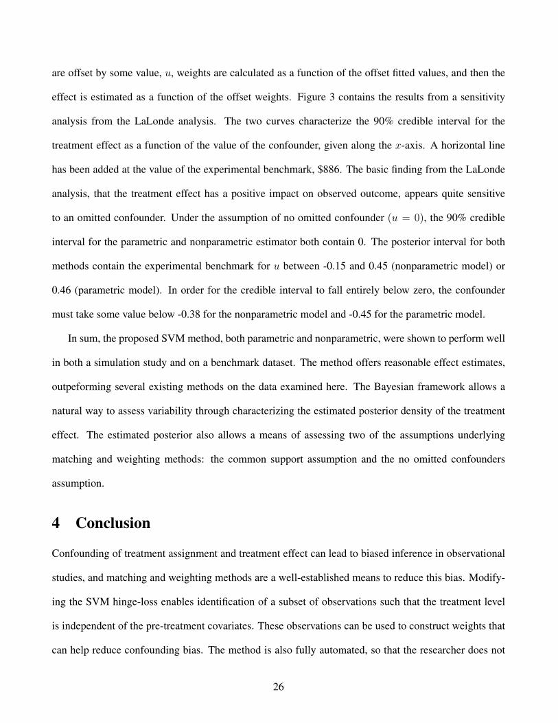
Sensitivity Analysis:90% Posterior Interval by Value of Unobserved Confounder

Figure 3: Sensitivity analysis using the LaLonde data. The two curves characterize the 90% posteriorcredible interval for the treatment effect as a function of the value of the confounder, given along thex-axis. A horizontal line has been added at the value of the experimental benchmark, $886. The basicfinding from the LaLonde analysis, that the treatment effect has a positive impact on observed outcome,appears quite sensitive to an omitted confounder. Under the assumption of no omitted confounder (u =0), the 90% posterior credible interval for the parametric and nonparametric estimator both contain 0.

Sensitivity Analysis Unobserved confounders pose an ineluctable problem to the applied researcher,

by definition. Best practice involves asking how big an unobserved confounder must be in order to affect

the subsequent inference on the outcome (Rosenbaum, 2002). As described above, the proposed method

allows a straightforward means for conducting a sensitivity analysis: the fitted values for a given model

25

are offset by some value, u, weights are calculated as a function of the offset fitted values, and then the

effect is estimated as a function of the offset weights. Figure 3 contains the results from a sensitivity

analysis from the LaLonde analysis. The two curves characterize the 90% credible interval for the

treatment effect as a function of the value of the confounder, given along the x-axis. A horizontal line

has been added at the value of the experimental benchmark, $886. The basic finding from the LaLonde

analysis, that the treatment effect has a positive impact on observed outcome, appears quite sensitive

to an omitted confounder. Under the assumption of no omitted confounder (u = 0), the 90% credible

interval for the parametric and nonparametric estimator both contain 0. The posterior interval for both

methods contain the experimental benchmark for u between -0.15 and 0.45 (nonparametric model) or

0.46 (parametric model). In order for the credible interval to fall entirely below zero, the confounder

must take some value below -0.38 for the nonparametric model and -0.45 for the parametric model.

In sum, the proposed SVM method, both parametric and nonparametric, were shown to perform well

in both a simulation study and on a benchmark dataset. The method offers reasonable effect estimates,

outpeforming several existing methods on the data examined here. The Bayesian framework allows a

natural way to assess variability through characterizing the estimated posterior density of the treatment

effect. The estimated posterior also allows a means of assessing two of the assumptions underlying

matching and weighting methods: the common support assumption and the no omitted confounders

assumption.

4 Conclusion

Confounding of treatment assignment and treatment effect can lead to biased inference in observational

studies, and matching and weighting methods are a well-established means to reduce this bias. Modify-

ing the SVM hinge-loss enables identification of a subset of observations such that the treatment level

is independent of the pre-treatment covariates. These observations can be used to construct weights that

can help reduce confounding bias. The method is also fully automated, so that the researcher does not

26

have to alternate between fitting a model and assessing balance, while the use of a nonparametric, smooth

basis helps relieve concerns over functional form assumptions.

The proposed method has been shown to perform well both in theory and in practice. In theory, the

proposed method has been shown to target the largest balanced subset of the data. Doing so maximizes

the power in the subsequent effect estimates. The Bayesian implementation allows a natural means

for assessing uncertainty in the effect estimate, as well as a means of assessing the common support

assumption and conducting a sensitivity analysis.

In practice, the proposed method performed well both on simulated and observational data. In the

simulation study, both SVM methods were resistant to the inclusion of irrelevant covariates–a problem

commonly encountered by the applied researcher who may have many potential confounders each with

either a small or negligible effect on treatment assignment. In observational data, the SVM methods

returned the lowest bias and, with a few exceptions, the lowest RMS error. Assessining the common

support assumption suggested why existing methods confront a negative bias in the observational data:

there appears a subset of individuals who both have an unusually large treatment effect and have very

few potential matches in the reservoir of controls. Broadly, across datasets and analyses, the nonpara-

metric method outperformed the parametric implementation, but the parametric method often compared

favorably to cutting-edge methods.

27

ReferencesAbadie, A. and Imbens, G. W. (2006). Large sample properties of matching estimators for average

treatment effects. Econometrica 74, 1, 235–267.

Abadie, A. and Imbens, G. W. (2008). On the failure of the bootstrap for matching estimators. Econo-

metrica 76, 6, 1537–1557.

Alvarez, R. M. and Levin, I. (2014). Uncertain neighbors: Bayesian propensity score matching for causal

inference. Working Paper.

Aronow, P. and Samii, C. (2013). Estimating average causal effects under interference between units.

Working Paper.

Austin, P. C. (2011). Optimal caliper widths for propensity-score matching when estimating differences

in means and differences in proportions in observational studies. Pharmaceutical Statistics 10, 2,

150–161.

Chipman, H. A., George, E. I., and McCulloch, R. E. (2010). BART: Bayesian additive regression trees.

Annals of Applied Statistics 4, 1, 266–298.

Cochran, W. G. (1968). The effectiveness of adjustment by subclassification in removing bias in obser-

vational studies. Biometrics 24, 295–313.

Cochran, W. G. and Rubin, D. B. (1973). Controlling bias in observational studies: A review. Sankhya:

The Indian Journal of Statistics, Series A 35, 417–446.

Cortes, C. and Vapnik, V. (1995). Support-vector networks. Machine Learning 20, 3, 273–297.

Crump, R., Hotz, V. J., Imbens, G., and Mitnik, O. (2009). Dealing with limited overlap in estimation of

average treatment effects. Biometrika 96, 1, 187–199.

Dehejia, R. H. and Wahba, S. (1999). Causal effects in nonexperimental studies: Reevaluating the

evaluation of training programs. Journal of the American Statistical Association 94, 1053–1062.

Diamond, A. and Sekhon, J. (2013). Genetic matching for estimating causal effects. Review of Econonics

and Statistics 95, 3, 932–945.

Friedman, J. (1991). Multivariate adaptive regression splines. The Annals of Statistics 19, 1, 1–67.

Friedman, J. H. and Fayyad, U. (1997). On bias, variance, 0/1-loss, and the curse-of-dimensionality.

Data Mining and Knowledge Discovery 1, 55–77.

28

Graham, B. S., Campos de Xavier Pinto, C., and Egel, D. (2012). Inverse probability tilting for moment

condition models with missing data. Review of Economic Studies 79, 3, 1053–1079.

Hainmueller, J. (2012). Entropy Balancing for Causal Effects: A Multivariate Reweighting Method to

Produce Balanced Samples in Observational Studies. Political Analysis 20, 1, 25–46.

Hastie, T., Rosset, S., Tibshirani, R., and Zhu, J. (2004). The entire regularization path for the support

vector machine. Journal of Machine Learning Research 5, 1391–1415.

Heckman, J. J., Ichimura, H., and Todd, P. (1997). Matching as an econometric evaluation estimator:

Evidence from evaluating a job training programme. Review of Economic Studies 64, 4, 605–654.

Hill, J., Weiss, C., and Zhai, F. (2011). Challenges with propensity score strategies in a high-dimensional

setting and a potential alternative. Multivariate Behavioral Research 46.

Ho, D. E., Imai, K., King, G., and Stuart, E. A. (2007). Matching as nonparametric preprocessing for

reducing model dependence in parametric causal inference. Political Analysis 15, 3, 199–236.

Ho, D. E., Imai, K., King, G., and Stuart, E. A. (2011). MatchIt: Nonparametric preprocessing for

parametric causal inference. Journal of Statistical Software 42, 8, 1–28.

Holland, P. W. (1986). Statistics and causal inference (with discussion). Journal of the American Statis-

tical Association 81, 945–960.

Iacus, S., King, G., and Porro, G. (2011). Multivariate matching methods that are monotonic imbalance

bounding. Journal of the American Statistical Association 106, 189–213.

Imai, K. and Ratkovic, M. (2014). Covariate balancing propensity score. Journal of the Royal Statistical

Society, Series B 76, 1, 243–263.

Kang, J. D. and Schafer, J. L. (2007). Demystifying double robustness: A comparison of alternative

strategies for estimating a population mean from incomplete data (with discussions). Statistical Sci-

ence 22, 4, 523–539.

Kimeldorf, G. S. and Wahba, G. (1971). Some results on Tchebycheffian spline functions. Journal of

Mathematical Analysis and Applications 33, 1, 82–95.

LaLonde, R. J. (1986). Evaluating the econometric evaluations of training programs with experimental

data. American Economic Review 76, 4, 604–620.

Lin, Y. (2002). Support vector machines and the Bayes rule in classification. Data Mining and Knowl-

edge Discovery 6, 259–275.

29

Lunceford, J. K. and Davidian, M. (2004). Stratification and weighting via the propensity score in

estimation of causal treatment effects: a comparative study. Statistics in Medicine 23, 19, 2937–2960.

McCaffrey, D. F., Griffin, B. A., Almirall, D., Slaughter, M. E., Ramchand, R., and Burgette, L. F. (2013).

A tutorial on propensity score estimation for multiple treatments using generalized boosted models.

Statistics in Medicine 32, 10, 3388–3414.

Mccaffrey, D. F., Ridgeway, G., and Morral, A. R. (2004). Propensity score estimation with boosted

regression for evaluating causal effects in observational studies. Psychological Methods 9, 403–425.

McCandless, L. C., Gustafson, P., Austin, P. C., and Levy, A. R. (2009). Covariate balance in a bayesian

propensity score analysis of beta blocker therapy in heart failure patients. Epidemiologic Perspectives

& Innovations 6, 5.

Miratrix, L., Sekhon, J., and Yu, B. (2012). Adjusting treatment effect estimates by post-stratification in

randomized experiments. Unpublished manuscript.

Neal, R. (2011). Mcmc using hamiltonian dynamics. In S. Brooks, A. Gelman, G. Jones, and X.-L.

Meng, eds., Handbook of Markov Chain Monte Carlo, CRC Handbooks of Modern Statistical Method.

Chapman and Hall.

Polson, N. and Scott, S. (2011). Data augmentation for support vector machines. Bayesian Analysis 6,

1, 1–24.

Ridgeway, G., McCaffrey, D., Morral, A., Burgette, L., and Griffin, B. A. (2014). Toolkit for weighting

and analysis of nonequivalent groups: A tutorial for the twang package. R Vignette.

Rosenbaum, P. R. (2002). Observational Studies. Springer-Verlag, New York, 2nd edn.

Rosenbaum, P. R., Ross, R. N., and Silber, J. H. (2007). Minimum distance matched sampling with fine

balance in an observational study of treatment for ovarian cancer. Journal of the American Statistical

Association 102, 477, 75–83.

Rosenbaum, P. R. and Rubin, D. B. (1983). The central role of the propensity score in observational

studies for causal effects. Biometrika 70, 1, 41–55.

Rosenbaum, P. R. and Rubin, D. B. (1985). Constructing a control group using multivariate matched

sampling methods that incorporate the propensity score. The American Statistician 39, 33–38.

Rubin, D. B. (1990). Comments on “On the application of probability theory to agricultural experiments.

Essay on principles. Section 9”. Statistical Science 5, 472–480.

30

Rubin, D. B. and Stuart, E. A. (2006). Affinely invariant matching methods with mixtures of ellipsoidally

symmetric distributions. Annals of Statistics 34, 4, 1814–1826.

Rubin, D. B. and Thomas, N. (1992). Affinely invariant matching methods with ellipsoidal distributions.

The Annals of Statistics 20, 1079–1093.

Scholkopf, B., Herbrich, R., and Smola, A. J. (2001). A generalized representer theorem. In Proceedings

of the Annual Conference on Computational Learning Theory, 416–426.

Scholkopf, B. and Smola, A. J. (2001). Learning with Kernels: Support Vector Machines, Regularization,

Optimization, and Beyond. MIT Press, Cambridge, MA, USA.

Sekhon, J. S. (2011). Multivariate and propensity score matching software with automated balance

optimization: The Matching package for R. Journal of Statistical Software 42, 7, 1–52.

Smith, J. and Todd, P. (2005). Does matching overcome LaLonde’s critique of nonexperimental estima-

tors? Journal of Econometrics 125, 1-2, 305–353.

Stuart, E. A. (2010). Matching methods for causal inference: A review and a look forward. Statistical

Science 25, 1, 1–21.

Wahba, G. (1990). Spline Models for Observational Data. SIAM, Philadelphia, PA, USA.

Wahba, G. (2002). Soft and hard classification by reproducing kernel Hilbert space methods. Proceedings

of the National Academy of Sciences 99, 26, 16524–16530.

Yang, D., Small, D., Silber, J., and Rosenbaum, P. (Forthcoming). Optimal matching with minimal

deviation from fine balance in a study of obesity and surgical outcomes. Biometrics .

Zigler, C. M. and Dominici, F. (2014). Uncertainty in propensity score estimation: Bayesian methods for

variable selection and model-averaged causal effects. Journal of the Americal Statistical Association

109, 505, 95–107.

31

A Proposition Proofs

PROOF 1 Joint Independence between Treatment Assignment and Covariates with a Binary Treatment

Assume η(·) such that sgn(E(T ∗i |Xi)) = sgn(η(Xi)) and η(·) is bounded, twice differentiable,

and lives in a reproducing kernel Hilbert space, H = H0 ⊕ H1, equipped with eigenfunctional bases1, ψj(·)

, eigenvalues

1, λj

, inner product < ·, · >H, and

∑j λ

2j < ∞. This implies η(Xi)

admits representation µ +∑

j αjψj(Xi). Denote η∗(Xi) =∑

j α∗jψ∗j (Xi), where ψ∗j (·) = ψj(·) −

E(ψj(·)|Ti = 1).

Take as the loss function E(|1 − T ∗i η∗(Xi)|+), andM the σ-algebra i : 1 − T ∗i η∗(Xi) > 0. The

first order condition after differentiating with respect to αj gives

E(T ∗i ψ

∗(Xi)|i ∈M)

= 0 (27)

⇒ E(ψ∗j (Xi)|i ∈M, Ti = 1

)= E

(ψ∗j (Xi)|i ∈M, Ti = 0

)= 0 (28)

⇒ E(η∗(Xi)|i ∈M, Ti = 1

)= E

(η∗(Xi)|i ∈M, Ti = 0

)= 0 (29)

⇒ E(η(Xi)|i ∈M, Ti = 1

)= E

(η(Xi)|i ∈M, Ti = 0

)= µ0, (30)

where the lines after the first follow from the centering of ψ∗j (·), the linearity of the expectation operator,

and the fact that η(·) and η∗(·) differ by only a constant, denoted µ0.

Next, noting that sgn(E(Ti|Xi)) = sgn(η(Xi)), equation 30 implies

E(|η(Xi)| · sgn(η(Xi))

∣∣i ∈M, Ti = 1)

=

E(|η(Xi)| · sgn(η(Xi))

∣∣i ∈M, Ti = 0)

= µ0 (31)

⇒ E(|η(Xi)|

∣∣Xi, i ∈M, Ti = 1)

=

E(− |η(Xi)|

∣∣Xi, i ∈M, Ti = 0)

= µ0 (32)

32

which clearly implies that η(Xi) = 0 for all i ∈ M and that µ0 = 0. Since η(Xi) is 0 overM, in this

region, Ti⊥⊥Xi.

In proving Ti⊥⊥Xi ⇒ i ∈ M, let B = i : Ti⊥⊥Xi, and define BM = i ∈ B⋂i ∈ M and

B∼M = i ∈ B⋂i ∈MC. Ti⊥⊥Xi ⇒ i ∈M is equivalent to B∼M = ∅.

Now, B∼M = ∅ implies there exists a region such that |1 − T ∗i η∗(Xi)|+ = 0 and Ti⊥⊥Xi. Since

the hinge-loss bounds the Bayes Risk from above (Wahba, 2002; Lin, 2002), this implies a Bayes Risk

for B∼M of zero. Since Ti⊥⊥Xi, Xi carries no information on Ti, so the classifier achieves Bayes Risk

1− P (T ∗i = sgn(E(T ∗i |i ∈ B∼M)

)= 1− p. This implies 1− p ≤ 0. p, a probability, cannot be greater

than 1 and p 6= 1, due to the common support assumption.

Therefore, there is an exact correspondence between marginal and balanced observations, asymptot-

ically.

Abstract Word Count:106

Body Word Count: 10,701

33