Bandwidth Prediction based on Nu-Support Vector Regression and

Bandwidth Prediction based on Nu-Support Vector Regression and ParallelHybrid Particle Swarm Optimization

Liang Hu 1 , Xilong Che 1∗, Xiaochun Cheng 2

1 College of Computer Science and Technology, Jilin University,No.2699 Qianjin Street, 130012, China.

E-mail: [email protected] (Liang Hu); [email protected] (Xilong Che)2 School of Computing Science, Middlesex University,

The Burroughs, Hendon, London NW4 4BT, England, UK.E-mail: [email protected]

Abstract

This paper addresses the problem of generating multi-step-ahead bandwidth prediction. Variation ofbandwidth is modeled as a Nu-Support Vector Regression (Nu-SVR) procedure. A parallel procedureis proposed to hybridize constant and binary Particle Swarm Optimization (PSO) together for optimizingfeature selection and hyper-parameter selection. Experimental results on benchmark data set show that theNu-SVR model optimized achieves better accuracy than BP neural network and SVR without optimiza-tion. As a combination of feature selection and hyper-parameter selection, parallel hybrid PSO achievesbetter convergence performance than individual ones, and it can improve the accuracy of prediction modelefficiently.

Keywords: bandwidth prediction; hyper-parameter selection; feature selection; nu-support vector regres-sion; parallel hybrid particle swarm optimization

1. Introduction

In the context of networks, bandwidth quantifies thedata rate that a network link or path can transfer.The bandwidth among computing nodes directly im-pacts application performance and quality of ser-vice. Growing complexity of distributed environ-ment is calling for accurate bandwidth prediction asdirection for package routing 1, congestion control2, bandwidth reservation 3, etc. The prediction stepalso extends from one-step-ahead 4 to multi-step-ahead 5.

This research focuses on modeling and optimiz-

ing methodologies for bandwidth prediction. Weconsider variation of bandwidth as a time series re-gression procedure that exploits the relationship be-tween past observation and future prediction. Re-gression is a feasible way proved by many re-searches 3,5,6 and our previous investigation 7.

We would like to further discuss the model opti-mization issues including hyper-parameter selectionand feature selection. Main contributions of this pa-per are as follows:

• to validate nu-support vector regression as methodto model multi-step-ahead bandwidth prediction;

∗Corresponding Author.

International Journal of Computational Intelligence Systems, Vol.3, No. 1 (April, 2010), 70-83

Published by Atlantis Press Copyright: the authors 70

zegerkarssen

Texte tapé à la machine

Received: 18-12-2008 Accepted: 27-11-2009

L. Hu et al

• to propose a parallel hybrid particle swarm op-timization algorithm to jointly perform hyper-parameter selection and feature selection;

• to introduce an accuracy and efficiency based cri-terion for model evaluation of bandwidth predic-tion.

The rest of this literature is organized as fol-lows: Section 2 provides a brief overview of relatedworks. Section 3 illustrates the modeling methodof bandwidth prediction in details. Section 4 givesthe parallel hybrid optimizing strategy consideringboth hyper-parameter selection and feature selec-tion. Section 5 proceeds prediction experiments onbenchmark data set and discusses comparative re-sults. Section 6 closes with conclusions as well asdirections for future research.

2. Related Works

The importance of bandwidth prediction has at-tracted efforts from a large number of researchers.Many algorithms have been presented in modelingbandwidth variation. Linear models can be imple-mented easily and fitted efficiently, therefore theyare adopted as prediction methods in many projects.Resource Prediction System (RPS) 6 is a famousproject in which bandwidth is modeled using lin-ear time series models, including AR (purely au-toregressive), MA (purely moving average), ARMA(autoregressive moving average), ARIMA (autore-gressive integrated moving average), and ARFIMA(autoregressive fractionally integrated moving av-erage). These models are also verified in the re-search of Yao et al. 8. Another well known sys-tem for network prediction is the Network WeatherService (NWS) 4. Wolski et al. comparedthe performance of forecasts generated using SNP(Semi Nonparametric Time Series Analysis), withthe techniques implemented by the NWS, such asRUN AVG (running average), LAST (last measure-ment), MEDIAN (median filter), GRAD (stochasticgradient) and so on. In the research of Nicholson 9,Markov model is employed in BreadCrumbs projectfor forecasting connectivity.

However, linear models are incapable of han-dling nonlinear conditions which exist in most of

applications. As a nonlinear pioneer of intelligentmethods, Artificial Neural Networks (ANNs) wereintroduced by many researchers in modeling band-width prediction. Liu et al. 2 designed an ANN pre-dictor which can predict the bursty available band-width for ABR traffic. Eswaradass et al. 10 proposedan ANN based approach for network performanceprediction, tested the ANN mechanism on classi-cal trace files and compared its performance withthe NWS system. Experimental results showed theANN approach always provides an improved predic-tion over that of NWS. Recurrent neural networksare also employed in several network applications11,12. However, the structures of neural networksare given directly by experience in these ANN re-searches, and there is not analytic mechanism to en-sure these structures suitable for other applications.Besides, there is an inherent limitation in ANNs forthe reason that ANN models are based on Empiri-cal Risk Minimization (ERM) principle 13, which isshort of overcoming under-fitting or over-fitting.

As a promising solution to nonlinear regres-sion problems, Support Vector Machines (SVMs)14 have recently been winning popularity due totheir remarkable characteristics such as good gen-eralization performance, the absence of local min-ima and sparse representation of the solution. Unlikethe ERM principle commonly used in conventionalregression techniques, SVM was proposed basedon Structural Risk Minimization (SRM) principle,which tries to control model complexity as well asthe upper bound of generalization risk, rather thanminimizing the training error only, thus is expectedto achieve better performance.

In the research of Mariyam et al. 15, SVM is em-ployed to predict TCP throughput. Available band-width, queuing delay, and packet loss are chosenas input features and throughput as output label.They also compared the accuracy of SVM predic-tor to linear History-Based (HB) predictor 16 andindicated superior performance. They emphasizedthe importance of feature selection on preventingover-fitting, but they only chose features accordingto experience rather than selection strategy. Theyused cross-validation 17 to select parameters for pre-diction models, nevertheless, two parameters were


Bandwidth Prediction Nu-SVR PH-PSO

selected separately rather than jointly, which willlead to performance degradation. Huang et al. 3

performed SVM and Particle Swarm Optimization(PSO) separately in building predictors so as to con-trol utility of resource, it is in fact a simple applica-tion of the two methods, which means no further im-provement is discussed to enhance the model’s per-formance.

Prem and Raghavan 5 have also explored the pos-sibility of applying SVM on bandwidth prediction,and indicated that the SVMs prediction are more ac-curate and outperform the classical methods such asAutoregressive based ones and Mean/Median basedones. However, there are still shortages in their re-search that deserve further discussion:

• the number of sample features reaches to 40, butthere is no feature selection method employed,thus resulting in a huge storage space and a longtraining time;

• no pretreatment strategy is announced. Samplevalues with big metric will bring numerical diffi-culties during calculation and lead to high regres-sion error;

• they achieve q-step-ahead prediction based on(q−1)-step-ahead prediction. It is usually impos-sible to control prediction accuracy within suchiterative mechanism;

• the hyper-parameters of prediction model aregiven directly without selection procedure, whichwill lower the generalization performance of pre-diction model.

In our previous work 7, we have proposed asearch strategy to select hyper-parameters, however,feature selection is not taken into consideration. Inthis paper, we attempt to introduce an evolutionaryalgorithm in optimizing bandwidth prediction modelfor the expectation of achieving high efficiency andlow error. The motivation of choosing and improv-ing the PSO is owing to its superior performanceamong evolutionary-based optimization algorithms18 and wide adaptability in many practical applica-tions.

3. Modeling Prediction with Nu-SVR

3.1. Prediction problem statement

Predicting bandwidth variation is a kind of regres-sion procedure as far as its essence is concerned.Bandwidth of a link bd can be expressed by bd(t)because its state value varies dynamically, such val-ues are monitored and recorded to form bandwidthtime series, denoted as Z = {zu}U

u=1, where zu ∈R,U ∈ N. Let zt stand for value of current time,then Z− = {zu}t

u=1, Z+ = {zu}Uu=t+1 can be used to

represent history set and future set separately, wheret ∈ (1,U). We define F : Z− → Z+ as predictionfunction set, then any element f ∈ F is a predictionfunction. In this research, we focus on q-step-aheadprediction function, its definition is given in Eq. (1).

f : zt+q = f (zt ,zt−1,zt−2, ...,zt−m+1).q,m ∈ N (1)

The prediction framework is schematicallyshown in Fig. 1. The bandwidth data set is di-vided into three parts: training set, validation setand test set. The training set is used to build pre-diction model, which is optimized using validationset and evaluated using test set. The model takeshistorical data as input and generates prediction forfuture variation.

Training set Validation set Test set

History Bandwidth Prediction Model Future

Train Optimize Test

Fig. 1. Prediction framework.

3.2. Data pretreatment

Spot set of time series Z = {zu}Uu=1 can’t

feed prediction model directly, therefore wetransform it into standard sample set (with


L. Hu et al

full features) G, detailed as follows: G ={zt ,zt−q,zt−q−1,zt−q−2, ...,zt−q−m+1}U

t=q+m, it can berewritten as G = {zi+q+m−1,zi+m−1,zi+m−2, ...,zi}l

i=1,l =U−q−m+1, where zi+q+m−1 is the labeled out-put value, (zi+m−1,zi+m−2, ...,zi) is the vector of minput features and l is the number of samples in G.It is in fact a segmentation based on overlapped timewindows with equal length, as is shown in Fig. 2.

Furthermore, it is necessary to scale data be-fore applying Nu-SVR method on them: feature val-ues in greater numeric ranges will dominate thosein smaller ones; values with large attribute maycause numerical difficulties during calculation andlead to malfunction of Nu-SVR’s kernel functionswhich are usually hypersensitive in a narrow inter-val. Let G

′= {yi,Xi}l

i=1 denote the scaled sampleset, where yi = z

′i+q+m−1 is a labeled value, Xi =

(z′i+m−1,z

′i+m−2, ...,z

′i) is a vector containing m fea-

tures. Scaling and unscaling function are expressedas Eq. (2) and (3).

z′= g(z) =

(ub− lb)(z− zmin)zmax− zmin + lb (2)

z = g−1(z′) =

(zmax− zmin)(z′− lb)

ub− lb+ zmin (3)

Where z is original value, z′

is scaled value indestination interval [lb,up] with lb as lower boundand ub as upper bound; zmax is the maximum valueof Z, and zmin is the minimum value of Z.

3.3. Modeling with Nu-SVR

With the pretreated sample set G′= {(yi,Xi)}l

i=1 ,where Xi ∈ Rm is the i-th vector containing m inputfeatures and yi ∈R is the corresponding desired out-put label, then modeling is achieved by training aregression function f :

f : Xi 7→ yi (4)

Nu-SVR 19 is a new regression version of SVM.In the following, we will explain in detail how to ap-ply its theory for prediction in the modeling stage.

To understand such method, we start from buildingprediction model using linear regression function:

y = f (X) = wT X +b (5)

Where w is the weight vector corresponding toX , and b is the bias. The generalization performanceof such linear function f (X) is fairly limited and un-able to reflect the true regression procedure. In orderto overcome such weakness, a standard mathemati-cal solution is the introduction of ϕ(X), which is anonlinear mapping function from the input space toa higher dimensional feature space. For example,let’s assume that X = ( j,k), then we can augment itwith ϕ(X) = ( j,k, j2,k2, jk). By using ϕ(X), we canreach to infinite dimensions for a more expressivef . However, it seems computationally impossible inthat case. In fact, we don’t have to compute ϕ(X)at all, we just need to compute the inner productϕ(Xi)T ϕ(X j) instead, such artful mechanism will beillustrated latter in this subsection. With the help ofϕ(X), linear regression function Eq. (5) is extendedto nonlinear function Eq. (6):

y = f (X) = W T ϕ(X)+b (6)

Where W is the weight vector corresponding toϕ(X). Based on the SRM principle of SVM, ourgoal is to estimate the coefficients (W and b) fol-lowing two rules at the same time: first, in order toachieve best performance, f (Xi) should be as closeas possible to the truth yi for all training samples;second, in order to prevent over-fitting, f (X) shouldbe as flat as possible. Then we arrive at how to mea-sure the “closeness” and “flatness”.

ε-insensitive loss function Lε is introduced tomeasure such “closeness”, as in Eq. (7). It measuresthe absolute error between prediction and true value,but with a tolerance of ε . If f (X) is in the tolerancerange of y± ε , no loss is considered; if a samplefalls out of such range, the distance between sam-ple and ε tube is denoted by slack variables ζi andζ ∗i , as is illustrated by Fig. 3. On the other hand,the parameter norm of f (X) is ||W ||2 = W TW , it isused to measure the “flatness”: smaller norm meanssmoother function.



Z zU zU−1 zU−2 ... zU−q zU−q−1 zU−q−2 ... zU−q−m+1 zU−q−m zU−q−m−1 ... z11st sample: ◦ • • • • •2nd sample: ◦ • • • • •3rd sample: ◦ • • • • •..th sample:

Figure 2: Creation of sample set.

Lε =

{0 |yi− f (Xi)|6 ε,

|yi− f (Xi)|− ε elsewhere.(7)

x

x

xx

x

xxx

x

xx

x

x

x

+ε−ε

x

ξ+ε

−ε0

ξ

Fig. 3. Theory of slack variable.

Hence we need to minimize the empirical error(overall loss on the training set) ∑l

i=1 Lε(yi, f (Xi))and the parameter norm ||W ||2 at the same time,which is equivalent to the following programmingproblem, namely primal problem of SVR:

min12

W TW +C1l

l

∑i=1

(ζi +ζ ∗i )

s.t.

(W T ϕ(Xi)+b)− yi 6 ε +ζi,

yi− (W T ϕ(Xi)+b) 6 ε +ζ ∗i ,

ζi,ζ ∗i > 0, i = 1, ..., l.

(8)

Where C is the regularized constant determiningthe trade-off between the empirical error and the pa-rameter norm. We still face the problem of choosingan adequate parameter ε in order to achieve goodperformance. Scholkopf 19,20 modified Eq. (8) suchthat ε also becomes a variable of the problem, andintroduced an extra term ν (nu) which attempts tominimize ε . To be more precise, they proved that νis an upper bound on the fraction of margin errors

and a lower bound on the fraction of support vec-tors. In addition, with probability 1, asymptotically,ν equals to both fractions. Accordingly Eq. (8) isadapted as follows, namely primal problem of Nu-SVR:

min12

W TW +C(νε +1l

l

∑i=1

(ζi +ζ ∗i ))

s.t.

(W T ϕ(Xi)+b)− yi 6 ε +ζi,

yi− (W T ϕ(Xi)+b) 6 ε +ζ ∗i ,

ε,ζi,ζ ∗i > 0, i = 1, ..., l.

(9)

Here 06 ν 61. By introducing Lagrange multi-pliers α,α∗,η ,η∗,β , a Lagrange function L is con-structed as follows:

L(α,α∗,η ,η∗,β ) =

12

W TW +Cνε +C1l

l

∑i=1

(ζi +ζ ∗i )−l

∑i=1

(ηiζi +η∗i ζ ∗i )−l

∑i=1

αi(ε +ζi + yi−W T ϕ(Xi)−b)−l

∑i=1

α∗i (ε +ζ ∗i − yi +W T ϕ(Xi)+b)−βε

(10)

It is understood that the Lagrange multipliersin Eq. (10) have to satisfy positive constraints, i.e.α(∗)

i ,η(∗)i ,β > 0. Here (∗) means condition with or

without ∗. It follows from the saddle point condi-tion that the partial derivatives of L with respect tothe primal variables (W,ε,b,ζ (∗)

i ) have to vanish foroptimality:


L. Hu et al

∂W L = 0→W =l

∑i=1

(αi−α∗i )ϕ(Xi)

∂bL = 0→l

∑i=1

(αi−α∗i ) = 0

∂εL = 0→Cν−l

∑i=1

(αi +α∗i )−β = 0

∂ζ (∗)i

L = 0→ Cl−α(∗)

i −η(∗)i = 0

(11)

Substituting function Eq. (11) into functionEq. (9) yields the following programming problem,namely dual problem of Nu-SVR:

min12

l

∑i, j=1

(α∗i −αi)Qi j(α∗

j −α j)−

l

∑i=1

yi(α∗i −αi)

s.t.

l

∑i, j=1

(α∗i −αi) = 0,

0 6l

∑i, j=1

(α∗i +αi) 6 Cν ,

0 6 α∗i ,αi 6 C

l, i = 1, ..., l.

(12)

Where Q denotes the matrix of kernel functions,with Qi j = K(Xi,X j) = ϕ(Xi)T ϕ(X j) as kernel func-tion. It can be seen from Eq. (12) that the Lagrangemultipliers ηi,η∗i ,β have been eliminated already.In order to solve such dual problem, we just need tocompute the inner product ϕ(Xi)T ϕ(X j) instead ofϕ(X) itself. Substituting W = ∑l

i=1(αi−α∗i )ϕ(Xi)

and Qi j = K(Xi,X j) = ϕ(Xi)T ϕ(X j) into Eq. (6)yields the prediction function:

y = f (x) =l

∑i=1

(αi−α∗i )K(Xi,X)+b (13)

This is the so-called support vector expansion.Based on the Karush-Kuhn-Tucker (KKT) 21,22 con-ditions of Quadratic Programming (QP) problem,

only a number of coefficients (αi−α∗i ) will be as-

sumed nonzero. Accordingly, the data samples asso-ciated with them are referred to as Support Vectors(SVs), which have the approximation errors equal toor larger than ε . According to Eq. (13), it is evidentthat support vectors are the only samples in trainingset that are used in determining the prediction func-tion f (X). The prediction function structure of SVMis given in Fig. 4.

f(X)

(X1) (X2) (X) (Xn-1) (Xn)

X1 X2 X Xn-1 Xn

K(X2, X)K(X1, X) K(Xn-1, X) K(Xn, X)

Fig. 4. Prediction function structure of SVM.

3.4. Kernel functions

In the prediction model achieved above, kernel func-tion Qi j = K(Xi,X j) = ϕ(Xi)T ϕ(X j) is introducedto compute inner product of augmented samples.It decides the complexity of prediction function,therefore affects the performance of Nu-SVR model.There are four kernel functions frequently used:

(a) Polynomial Function (PF):K(Xi,X j) = (γ(XT

i X j)+a)b,γ > 0,a ∈ R,b ∈ N;

(b) Radial Basis Function (RBF):K(Xi,X j) = exp(−γ||Xi−X j||2),γ > 0;

(c) Sigmoid Function (SF):K(Xi,X j) = tanh(γ(XT

i X j)− c),γ > 0,c ∈ R;

(d) Linear Function (LF):K(Xi,X j) = XT

i X j.

In general, RBF kernel is a reasonable firstchoice in training SVM. According to research ofKeerthi and Lin 23, RBF kernel with certain parame-ters can get same performance as LF and SF kernel.



Unlike LF kernel, it nonlinearly maps samples intoa higher dimensional space, so it can handle the casewhen the relation between class labels and attributesis nonlinear. Values of PF kernel may go to infin-ity or zero when the degree is large, in contrast toRBF kernel of which key point is from zero to one.Therefore, RBF has less numerical difficulties. Inaddition, it has less hyper-parameters (only γ) whichinfluence the complexity of model selection than PFkernel. Therefore, RBF kernel is our choice in train-ing SVMs. It is clear that once hyper-parameters ofmodel and features of samples are selected, Eq. (13)is achievable by evaluating (αi−α∗

i ) and b. Libsvmtoolkit 24 is employed to solve such QP problem.

4. Optimizing Prediction with PH-PSO

Generalization performance of prediction model re-lies directly on the choice of hyper-parameters. Inaddition, irrelevant features in samples will alsospoil the accuracy and efficiency of model. Be-sides, hyper-parameter selection and feature selec-tion also correlate with each other. Accordingly, theoptimization problem concerning the two is codedwith a hybrid vector PR, which consists of real num-bers and binary numbers. As Nu-SVR is able to se-lect ε by itself, only C and γ are considered hyper-parameters. The value 1 or 0 for b fs, respectively,stands for whether the corresponding feature in sam-ples is selected. With [C−,C+], [γ−,γ+] as the valueintervals and Fit(•) as the target function, the com-binational optimization concerning hyper-parameterselection and feature selection jointly can be ex-pressed as:

max Fit(PR)

s.t.

PR = {C,γ,b f1,b f2, ...,b fm},C ∈ [C−,C+],γ ∈ [γ−,γ+],

b fs ∈ {0,1},s = 1,2, ...,m.

(14)

Because PSO is powerful, easy to implement,and computationally efficient, it is employed andadapted to optimize our prediction model. PSO wasproposed by Dr. Kennedy and Dr. Eberhart in1995 25, inspired by social behavior of nature sys-tem, such as bird flocking or fish schooling. There

are mainly two types of PSO distinguished by dif-ferent updating rules for calculation of particles’ po-sition and velocity: continuous version 25,26 and dis-crete version 27. Concerning characteristics of ourproblem, this study proposes a combinational op-timization algorithm which hybridizes continuousPSO and discrete PSO together, in hope of improv-ing performance of prediction model, as is explainedin details:

The system is initialized with a population ofrandom particles and searches a multi-dimensionalsolution space for optima by updating particle gen-erations. Each particle moves based on the directionof local best solution discovered by itself and globalbest solution discovered by the swarm. Each parti-cle calculates its own velocity and updates its posi-tion in each iteration until the termination conditionis met. Supposing P particles in a D-dimensionalsearch space:

(a) AP×D denotes the position matrix of all parti-cles, p = 1,2, ...,P,d = 1,2, ...,D, row vectorap in A denotes the position of the p-th parti-cle, recorded as ap = {ap1,ap2, ...,apD};

(b) VP×D denotes the velocity matrix of all par-ticles, row vector vp in V denotes the ve-locity of the p-th particle, recorded as vp ={vp1,vp2, ...,vpD};

(c) LBP×D denotes the local best position of allparticles, row vector lbp in LB denotes the lo-cal best position of the p-th particle, recordedas lbp = {lbp1, lbp2, ..., lbpD};

(d) Row vector gb = {gb1,gb2, ...,gbD} denotesthe global best position shared by all particles.

The particle is represented by the hybrid vectorPR. During each iteration the real and binary parts ofPR are updated jointly using different rules, namelyEq. (15) and Eq. (16) for real part and Eq. (17) forbinary part.

vpd(t +1) = w× vpd(t)+

c1× rdm1(0,1)× (lbpd(t)−apd(t))+

c2× rdm2(0,1)× (gbd(t)−apd(t)).

apd(t +1) = apd(t)+ vpd(t +1).

(15)


L. Hu et al

apd =

Amin apd < Amin;apd Amin < apd < Amax;Amax apd > Amax.

vpd =

−V max vpd <−V max;vpd −V max < vpd < V max;V max vpd > V max.

(16)

vpd(t +1) = w× vpd(t)+

c1× rdm1(0,1)× (lbpd(t)−apd(t))+

c2× rdm2(0,1)× (gbd(t)−apd(t)).

i f (rdm(0,1) < Sg(vpd(t +1)))

then apd(t +1) = 1,

else apd(t +1) = 0;

Sg(v) =1

1+ e−v .

(17)

The problem-dependent constants Amin, Amax andV max are defined in order to clamp the excessiveroaming of particles, as in Eq. (16). V max is an im-portant parameter. It determines the resolution, orfineness, with which regions between the presentposition and the target (best so far) position aresearched. If V max is too high, particles may fly pastgood solutions. On the other hand, if V max is toosmall, particles may be short at exploring ability andtrapped in local optima. The relationship betweenvelocity and position is illustrated by Fig. 5.

apd(t+1)

apd(t)

gbd(t)

lbpd(t)c1 rdm1(0,1) (lbpd(t)-apd(t))

c2 rdm2(0,1) (gbd(t)-apd(t))

w vpd(t) vpd(t+1)

Fig. 5. Relationship between velocity and position.

rdm(0,1), rdm1(0,1) and rdm2(0,1) are randomnumbers evenly distributed, respectively, in [0,1]. t

denotes the step of iteration. Inertia weight w playsthe role of balancing global search and local search,it can be a positive constant or even a positive lin-ear/nonlinear function of time. Acceleration con-stant c1 and c2 represent personal and social learningfactors, respectively; if c1 = 0, then the particle onlyhas social experience, it may converge fast but fallinto local minima easily; if c2 = 0, then the parti-cle only has personal experience, all particles in theswarm become moving by themselves without inter-action, thus the probability of finding best solutionis very little; if c1 = c2 = 0, then the particle doesnot have any experience, all particles in the swarmbecome disorderly and unsystematic. Sg(•) is a sig-moid function limiting transformation.

Fitness definition. The definition of fitnessfunction is crucial in that it determines what a PSOshould optimize. Besides, the particle with high fit-ness value has high probability to effect other’s posi-tions during iterations. Accuracy and efficiency areboth concerned in evaluating the fitness of predictionmodel, in other words, a model is better (with largerfitness) only if it has lower prediction error as wellas less training time, thus comes to a relationshipof symmetrical inverse proportion. Moreover, whenthe training time is acceptable, accuracy is consid-ered prior, so we design the fitness function usingEq. (18). Where MSEt is the training mean squarederror, h is a constant controlling the bound of fitnessand Tt denotes the model’s training time.

Fitness =h

MSEt × lnTt

MSEt =1l

l

∑i=1

(yi− f (Xi))2(18)

Cross-Validation. There are three commonways of calculating MSEt : cross-validation 17, full-validation 7 and leave-one-out (LOO) 28. In r-foldcross-validation, the validation set is divided intor subsets of equal size. Sequentially one subsetis tested using the model trained on the remain-ing (r − 1) subsets. Thus, each instance of thewhole validation set is predicted once so the cross-validation accuracy is the mean squared error in to-tal.

Full-validation is an extreme of the r-fold cross-



validation when r is 1. In full-validation, the entirevalidation set is used as training set, and also usedas test set. Whereas, LOO is another extreme of ther-fold cross-validation when r equals l, l is the totalsample number of validation set.

In full-validation, model training is performedonce only so that computational time is short. How-ever, prediction error is estimated using seen sam-ples, which makes it impossible to reflect model’sgeneralization performance on unseen samples. Onthe contrary, LOO makes full use of seen samples topredict unseen ones, yet computational time is toolong in that model training has to be performed ltimes. Traditional 5-fold cross-validation is a trade-off between the two, so that it is chosen as errorestimation method in fitness calculation.

Finish

Termination condition ?

Yes

No

Initialize system

Update local best/global best

Update

velocity

and

position

Preprocessing

Fitness evaluation

Preprocessing

Fitness evaluation

Preprocessing

Fitness evaluation

Preprocessing

Fitness evaluation

Preprocessing

Fitness evaluation

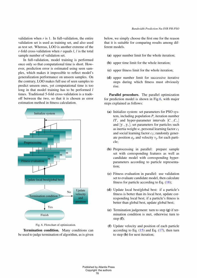
Fig. 6. Flowchart of optimization.

Termination condition. Many conditions canbe used to judge termination of algorithm, as is given

below, we simply choose the first one for the reasonthat it is suitable for comparing results among dif-ferent models.

(a) upper number limit for the whole iteration;

(b) upper time limit for the whole iteration;

(c) upper fitness limit for the whole iteration;

(d) upper number limit for successive iterativesteps during which fitness must obviouslyrise.

Parallel procedure. The parallel optimizationfor prediction model is shown in Fig.6, with majorsteps explained as follows:

(a) Initialize system: set parameters for PSO sys-tem, including population P, iteration numberIT , and hyper-parameter intervals [C−,C+]and [γ−,γ+]; set parameters for particles suchas inertia weight w, personal learning factor c1and social learning factor c2; randomly gener-ate position ap and velocity vp for each parti-cle;

(b) Preprocessing in parallel: prepare sampleset with corresponding features as well ascandidate model with corresponding hyper-parameters according to particle representa-tion;

(c) Fitness evaluation in parallel: use validationset to evaluate candidate model, then calculatefitness for particle according to Eq. (18);

(d) Update local best/global best: if a particle’sfitness is better than its local best, update cor-responding local best; if a particle’s fitness isbetter than global best, update global best;

(e) Termination judgement: turn to step (g) if ter-mination condition is met, otherwise turn tostep (f);

(f) Update velocity and position of each particleaccording to Eq. (15) and Eq. (17), then turnto step (b) for next iteration;


L. Hu et al

(g) Finish: output global best, prepare sample setwith selected features and prediction modelwith selected hyper-parameters according torepresentation of global best.

5. Experiments and Discussions

After the presentation of modeling and optimizingmechanisms, the following questions have furthermotivated us for experiments.◦ Is the model feasible for one-step-ahead pre-

diction or multi-step-ahead prediction ?• We compare different models for q-step-ahead

bandwidth prediction, q = 1,2,3,4,5 are concerned.◦ Are the efficiency and accuracy acceptable ?•We log parallel/serial CPU time for optimizing

models, and employ Mean Absolute Error (MAE) tomeasure prediction accuracy, as in Eq. (19), where zand z∗ denote true value and predicted value in orig-inal interval. We also implement Back PropagationNeural Network (BPNN) for comparison.

MAE =1l

l

∑i=1|z− z∗| (19)

◦ Are there remarkable differences among opti-mizing strategies ?• We implement four different strategies includ-

ing feature selection with hyper-parameter selection(FH), feature selection without hyper-parameter se-lection (F0), hyper-parameter selection without fea-ture selection (0H), and parameters given directlywithout any optimization mechanism, same way asin 5 (00).◦ Does the optimizing procedure converge dur-

ing proper iterations ?• We record the iteration number and corre-

sponding global best fitness to evaluate convergenceof optimizing procedure.

5.1. Preparations for experiments

Experiment nodes are running under Fedora CoreLinux 9.0 system and connected by 100MB switch-hub. Each node is equipped with single Intel Pen-tium IV 3.0GHz CPU and 1GB-DDR400Hz MEM-ORY. One node is used to control the overall opti-

mizing procedure, and the rest nodes are used forfitness evaluation in parallel. The number of nodesused for fitness evaluation is equal to the number ofparticles in PH-PSO algorithm. The control programand optimizing programs are coded in java, and de-ployed on different nodes in the form of web service.All the tests are implemented through dynamic col-laboration of such services.

Table 1. Statistics of data sets.

General statistic valueSet size 1511Minimum 3.05Maximum 334.0Mean 85.14908008Variance 1932.83648856

For the purpose of giving comparable and repro-ducible results, we prefer using public data ratherthan historical data recorded by ourselves. We chose“iepm-bw.bnl.gov.iperf” 29 as benchmark data set.It is published by the Stanford Linear AcceleratorCenter, University of Stanford. After pretreatmentto original data, the latest 200 samples are sequen-tially chosen to form experiment data set, which isthen divided into training set, validation set and testset, with a proportion of 100:50:50. Summary statis-tics for data set are listed in Table. 1.

Table 2. Parameters initialization.

parameter value description[lb,up] [0,1] destination intervalm 10 number of full featuresν 0.54 extra term for minimizing ε[γ−,γ+] [2−10,210] parameter for RBF kernel[C−,C+] [2−10,210] regularized term for SVRw 1.4→ 0.5 inertia weight for PSOc1,c2 2,2 acceleration constants for PSOIT 100 iteration times for PSOP 10 number of particles for PSOh 0.01 fitness constant for PSObpIn 10 input number for BPNNbpHid 5 hidden number for BPNNbpOut 1 output number for BPNNsteps 500 train steps for BPNN



1 2 3 4 517

18

19

20

21

22

23

axis q−step−ahead

axis

MA

E (

Mbp

s)

MAE results (Zoom out)

F00HFH00BP

(a) MAE(Zoom Out)

1 2 3 4 517.6

17.7

17.8

17.9

18

18.1

axis q−step−aheadax

is M

AE

(M

bps)

MAE results (Zoom in)

F00HFH00

(b) MAE(Zoom In)

1 2 3 4 50

10

20

30

40

50

60


axis

SV

num

ber

SV results (bandwidth)

F00HFH00

(c) number of SVs

Figure 7: prediction models.

Parameters are also initialized with values thatare commonly used: fix ν based on the research of30, set acceleration constants c1 and c2 according to25, decrease inertia weight w linearly with time asproposed in 26, and change C,γ exponentially dur-ing optimization 31, detailed in Table.2.

5.2. Results and discussions

The MAE results of different models are shownin Fig. 7(a) and Fig. 7(b). For all q-cases, theSVMs achieve better accuracy than BPNN. MAEof SVMs stays below 17.9 Mbps, there is no re-markable difference between one-step-ahead predic-tion and multi-step-ahead prediction. As predictionstep q increases, there is not an obvious ascendingtrend in MAE on experiment data set, which meansthat our modeling method is suitable for both one-step-ahead and multi-step-ahead bandwidth predic-tion. Furthermore, comparing four strategies, theintroduction of optimizing mechanism helps to en-hance the accuracy of prediction model, especiallythe combinational optimization FH which achieveslower error in most of the q-cases.

A remarkable characteristic of SVR/Nu-SVR isthe sparse representation of the solution, namelymodel with less support vectors is better in achiev-ing same accuracy. It can be seen from Fig. 7(b)and 7(c) that Nu-SVR models being optimized havehigher accuracy than SVR model without optimiz-ing strategy, whereas support vector numbers of Nu-SVR models are over 50 compared to SVR whose

number is less than 10. We can see there is a tradeoffbetween model accuracy and solution sparseness:model with more support vectors are more compli-cated as well as more capable in characterization.

Four strategies are different in efficiency, the par-allel/serial CPU time of each is compared in Fig. 8.From each sub-figure, we can see that the CPUtime does not show a remarkable tendency as stepq increases. 0H costs more time than FH and F0,which means the model’s training time can be obvi-ously reduced by feature selection rather than hyper-parameter selection. From comparison between par-allel and serial time, it is clear that the introductionof parallelization can remarkably speed up the opti-mizing procedure, especially the combinational op-timization FH within 3 seconds for experiment dataset.

The global best fitness during each iteration islogged for convergence comparison, as is shown inFig. 9. FH wins the best fitness in all the q-caseswith 0H as the last, which implies that combina-tional optimization FH as a whole outperforms in-dividual optimization F0 or 0H. Landscape compar-ison among different q-cases are shown in Fig. 9(f),no obvious trend on fitness is found when predic-tion step q increases. From Sub-figures in Fig. 9 wecan count times that prematurity happens: 3 timesin F0, 5 times in 0H, and 2 times in FH. It is im-plied that the combinational optimization convergesduring proper iterations in most of the q cases.


L. Hu et al

1 2 3 4 51500

2000

2500

3000


axis

par

alle

lTim

e (m

s)

parallelTime results (bandwidth)

F00HFH

(a) parallelTime

1 2 3 4 51

1.5

2

2.5x 10

4

axis q−step−aheadax

is s

eria

lTim

e (m

s)

serialTime results (bandwidth)

F00HFH

(b) serialTime

Figure 8: Optimizing time.

0 50 100

0.16

0.18

0.2

0.22

0.24

axis iteration number

axis

fitn

ess

convergence results (bandwidth, q=1)

F00HFH

(a) q=1

0 50 100

0.16

0.18

0.2

0.22

0.24


axis

fitn

ess


F00HFH

(b) q=2

0 50 1000.16

0.18

0.2

0.22

0.24


axis

fitn

ess


F00HFH

(c) q=3

0 50 100

0.2

0.25

0.3

0.35


axis

fitn

ess


F00HFH

(d) q=4

0 50 100

0.16

0.18

0.2

0.22

0.24


axis

fitn

ess


F00HFH

(e) q=5

0 50 100

0.2

0.25

0.3

0.35


axis

fitn

ess

convergence results (bandwidth, FH)

q=1

q=2

q=3

q=4

q=5

(f) FH landscape

Figure 9: Convergence results.



6. Conclusions and Future works

In this paper, Nu-Support Vector Regression (Nu-SVR) is employed to model one-step-ahead andmulti-step-ahead bandwidth prediction. Model opti-mization issues including hyper-parameter selectionand feature selection are also discussed. A Paral-lel Hybrid Particle Swarm Optimization (PH-PSO)algorithm is proposed to improve the accuracy andefficiency of prediction model.

Prediction results shows that the SVMs achievebetter accuracy than BPNN. Mean Absolute Error(MAE) does not show remarkable ascending ten-dency while prediction step is growing, thereforeNu-SVR is feasible for modeling bandwidth pre-diction in not only one-step-ahead but also multi-step-ahead settings. Comparative results also indi-cate that optimizing time can be obviously reducedby feature selection rather than hyper-parameter se-lection. As a combination of feature selection andhyper-parameter selection, PH-PSO achieves betterconvergence performance than individual ones. Itcan improve the accuracy of prediction model inrather short time, namely less than 3 seconds.

Our future work will extend in two ways. First,there are still unsatisfied results that are calling forfurther improvements; for example, to prevent pre-maturity in optimizing procedure. Second, consid-ering the diversity of networks, more elements andapplication instances should be verified to supportthe feasibility of our methods.

Acknowledgments

This work is funded by: National Natural Sci-ence Foundation of China under Grant No.60873235&60473099 and by Science-TechnologyDevelopment Key Project of Jilin Province of Chinaunder Grant No. 20080318 and by Program of NewCentury Excellent Talents in University of China un-der Grant No. NCET-06-0300.

References

1. L. Dai, Y. Xue, B. Chang, Y. Cao, and Y. Cui, “Op-timal Routing for Wireless Mesh Networks With Dy-

namic Traffic Demand,” Mobile Netw Appl., 13, 97-116 (2008).

2. Z. X. Liu, X. P. Guan, and H. H. Wu, “Bandwidth pre-diction and congestion control for abr traffic based onneural networks,” Lecture Notes in Computer Science,3973/2006, 202–207 (2006).

3. C. J. Huang, Y. T. Chuang, W. K. Lai, Y. H. Sun, andC. T. Guan, “Adaptive resource reservation schemesfor proportional DiffServ enabled fourth-generationmobile communications system,” Comput. Commun.,30(7), 1613–1623 (2007).

4. R. Wolski, L. Miller, G. Obertelli, and M. Swany,“Performance Information Services for Computa-tional Grids,” In: Resource Management for GridComputing, J. Nabrzyski, J. Schopf, and J. Weglarz,editors, Kluwer Publishers, Fall (2003).

5. H. Prem and N. R. S. Raghavan, “A Support Vec-tor Machine Based Approach for Forecasting of Net-work Weather Services,” J. Grid Comput., 4(1), 89–114 (2006).

6. P. A. Dinda, “Design, Implementation, and Perfor-mance of an Extensible Toolkit for Resource Predic-tion in Distributed Systems,” IEEE Trans. ParallelDistrib. Syst., 17(2), 160–173 (2006).

7. L. Hu and X. L. Che, “Design and Implementation ofBandwidth Prediction based on Grid Service,” Proc.10th IEEE International Conference on High Per-formance Computing and Communications (HPCC-08, September 25-27, 2008, Dalian, China), 45–52(2008).

8. J. Yao, S. S. Kanhere, and M. Hassan, “An Empiri-cal Study of Bandwidth Predictability in Mobile Com-puting,” Proc. 3rd ACM International Workshop onWireless Network Tesbeds, Experimental Evaluationsand Characterization (WINTECH2008) in conjunc-tion with ACM MOBICOM2008, San Francisco, USA,September (2008).

9. A. J. Nicholson and B. D. Noble, “BreadCrumbs:forecasting mobile connectivity,” Proc. MOBI-COM08, 46–57 (2008).

10. A. Eswaradass, X. H. Sun, and M. Wu, “A neu-ral network based predictive mechanism for availablebandwidth,” Proc. 19th International Parallel andDistributed Processing Symposium (IPDPS05, April),33a (2005).

11. J. Zhang and I. Marsic, “Link quality and signal-to-noise Ratio in 802.11 WLAN with fading: ATime-Series Analysis,” Proc. IEEE 64th VehicularTechnology Conference (VTC-2006-Fall), Montreal,Canada, September, “Modeling and Simulation ofMobile Wireless Systems”, 1–5 (2006).

12. Gowrishankar and P. S. Satyanarayana, “Recurrentneural network based BER prediction for NLOS chan-nels,” Proc. 4th International Conference on MobileTechnology, Applications, and Systems and the 1st In-


L. Hu et al

ternational Symposium on Computer Human interac-tion in Mobile Technology (Mobility’07, Singapore,September 10-12), 410–416 (2007).

13. P. F. Pai, W. C. Hong, P. T. Chang, and C. T. Chen,“The application of support vector machines to fore-cast tourist arrivals in Barbados: An empirical study,”International Journal of Management, 23(2), 375–385(2006).

14. V. N. Vapnik, “The Nature of Statistical Learning The-ory,” 2nd ed, Springer-Verlag, New York (1999).

15. M. Mariyam, S. Joel, B. Paul, and X. J. Zhu, “A ma-chine learning approach to TCP throughput predic-tion,” Proc. 2007 ACM SIGMETRICS InternationalConference on Measurement and Modeling of Com-puter Systems (San Diego, California, USA, June 12-16), SIGMETRICS ’07, 97–108 (2007).

16. Q. He, C. Dovrolis, and M. Ammar, “On the pre-dictability of large transfer TCP throughput,” Proc.SIGCOMM’05 (Philadelphia, Pennsylvania, USA,August 21-26), 35(4), 145–156 (2005).

17. M. W. Browne, “Cross-validation methods,” Journalof Mathematical Psychology, 44(1), 108–132 (2000).

18. E. Elbeltagi, T. Hegazy, and D. Grierson, “Compar-ison among five evolutionary-based optimization al-gorithms,” Advanced Engineering Informatics, 19(1),43–53 (2005).

19. B. Scholkopf, A. J. Smola, R. C. Williamson, and P.L. Bartlett, “New support vector algorithms,” NeuralComputation, 12(5), 1207–1245 (2000).

20. A. J. Smola and B. Scholkopf, “A tutorial on supportvector regression,” Statistics and Computing, 14(3),199–222 (2004).

21. W. Karush, “Minima of functions of several variableswith inequalities as side constraints,” Masters thesis,Dept. of Mathematics, Univ. of Chicago (1939).

22. H. W. Kuhn and A. W. Tucker, “Nonlinear program-ming,” Proc. 2nd Berkeley Symposium on Mathemat-

ical Statistics and Probabilistics (Berkeley), 481–492(1951).

23. S. S. Keerthi and C. J. Lin, “Asymptotic behaviors ofsupport vector machines with Gaussian kernel,” Neu-ral Computation, 15(7), 1667–1689 (2003).

24. C. C. Chang and C. J. Lin, “LIBSVM: a li-brary for support vector machines,” Available:http://www.csie.ntu.edu.tw/˜cjlin/libsvm/ , May 1(2008).

25. J. Kennedy and R. C. Eberhart, “Particle swarmoptimization,” Proc. IEEE International Conferenceon Neural Networks (Perth,Australia), 4, 1942–1948(1995).

26. Y. Shi and R. C. Eberhart, “A modified particle swarmoptimizer,” Proc. IEEE International Conference onEvolutionary Computation, 69–73 (1998).

27. J. Kennedy and R. C. Eberhart, “A Discrete BinaryVersion of the Particle Swarm Optimization,” Proc.IEEE International Conference on Neural Networks(Perth, Australia), 5, 4104–4108 (1997).

28. K. Fukunaga and D. M. Hummels, “Leave-one-outprocedures for nonparametric error estimates,” IEEETransactions on Pattern Analysis and Machine Intel-ligence, 11(4), 421–423 (1989).

29. Bandwidth data set, Available:http://www.slac.stanford.edu/comp/net/iepm-bw.slac.stanford.edu/combinedata/. Aug 01 (2006).

30. A. Chalimourda, B. Scholkopf, and A. J. Smola, “Ex-perimentally optimal nu in support vector regressionfor different noise models and parameter settings,”Neural Networks, 17, 127–141 (2004).

31. C. W. Hsu, C. C. Chang, and C. J. Lin, “A prac-tical guide to support vector classification,” De-partment of Computer Science and InformationEngineering, National Taiwan University, Avail-able: http://www.csie.ntu.edu.tw/˜cjlin/papers/guide/guide.pdf (2003).


Date post:	03-Feb-2022
Category:	Documents
Upload:	others
View:	4 times
Download:	0 times

Bandwidth Prediction based on Nu-Support Vector Regression and

Documents