i Bank Lending to Rural vs. Urban Firms in the United States Before, During, and After the Great Financial Crisis by Rebel A. Cole, Ph.D. Krähenbühl Global Consulting Delray Beach, FL 33483 for Office of Advocacy U.S. Small Business Administration under contract number SBAHQ-17-M-0108 Release Date: May 5, 2020 This report was developed under a contract with the Small Business Administration, Office of Advocacy, and contains information and analysis that were reviewed by officials of the Office of Advocacy. However, the final conclusions of the report do not necessarily reflect the views of the Office of Advocacy.
Transcript
i
Bank Lending to Rural vs. Urban Firms in the United States
Before, During, and After the Great Financial Crisis
by
Rebel A. Cole, Ph.D. Krähenbühl Global Consulting
Delray Beach, FL 33483
for
Office of Advocacy U.S. Small Business Administration
under contract number SBAHQ-17-M-0108 Release Date: May 5, 2020
This report was developed under a contract with the Small Business Administration, Office of Advocacy, and contains information and analysis that were reviewed by officials of the Office of Advocacy. However, the final conclusions of the report do not necessarily reflect the views of the Office of Advocacy.
i
Table of Contents Executive Summary ........................................................................................................................ ii 1. Background ............................................................................................................................. - 4 - 2. Literature Review.................................................................................................................... - 6 -
2.1. Availability of Credit to Small Businesses ...................................................................... - 6 - 2.2. Availability of Credit to Rural Small Businesses .......................................................... - 10 -
6.1. Univariate Results ......................................................................................................... - 19 - 6.1.1. Amounts of Originations by Loan Size ...................................................................... - 19 - 6.1.2. Amounts of Originations to Firms with Revenues less than $1 Million .................... - 22 - 6.1.3. Numbers of Originations by Loan Size ...................................................................... - 24 - 6.1.4. Numbers of Originations to Firms with Revenues less than $1 Million .................... - 27 - 6.2. Multivariate Results ...................................................................................................... - 28 - 6.2.1. Descriptive Statistics .................................................................................................. - 29 - 6.2.2. Multivariate Regression Models of the Amount of Small-Business-Loan
Originations................................................................................................................ - 30 - 6.2.4. Multivariate Regression Models of the Number of Small-Business-Loan
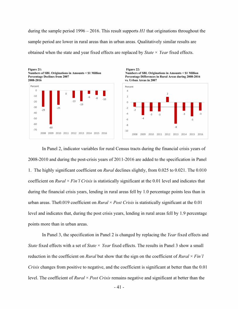
List of Figures Figure 1: SBL Originations < $100,000, Aggregate Dollar Amounts in Urban vs. Rural Areas ......... - 20 - Figure 2: SBL Originations $100,000-$1 Million, Aggregate Dollar Amounts in Urban vs. Rural Areas .. - 20 - Figure 3: SBL Originations per Capita, < $100,000, Average Dollar Amounts per Capita in Urban vs. Rural Areas .................................................................................................................................... - 20 - Figure 4: SBL Originations per Capita, $100,000-$1 Million, Average Dollar Amounts per Capita in Urban vs. Rural Areas ............................................................................................................................ - 20 - Figure 5: SBL Originations to Firms with Revenues < $1 Million, Aggregate Dollar Amounts in Urban vs. Rural Areas …… ........................................................................................................................... - 23 - Figure 6: SBL Originations to Firms with Revenues < $1 Million, Average Dollar Amounts per Capita in Urban vs. Rural Areas ........................................................................................................................... - 23 - Figure 7: SBL Originations < $100,000, Aggregate Number of Loans in Urban vs. Rural Areas ........ - 25 - Figure 8: SBL Originations $100,000-$1 Million, Aggregate Number of Loans in Urban vs. Rural Areas .. .................................................................................................................................... - 25 - Figure 9: SBL Originations < $100,000, Average Number of Loans per Capita in Urban vs. Rural Areas ….. ............................................................................................................................................ - 25 - Figure 10: SBL Originations $100,000-$1 Million, Average Number of Loans per Capita in Urban vs. Rural Areas - 25 - Figure 11: SBL Originations to Firms with Revenues < $1 Million, Number of Loans in Urban vs. Rural Areas ……………………...………………………………………………........................................... - 27 - Figure 12: SBL Originations to Firms with Revenues < $1 Million, Number of Loans per Capita in Urban vs. Rural Areas ....................................................................................................................................... - 27 - Figure 13: Amounts of SBL Originations < $1 Million, Percentage Declines ......................... ……………...32 Figure 14: Amounts of SBL Originations < $1 Million, Percentage Differences in Rural vs. Urban Areas .. ……………... .................................................................................................................. 32 Figure 15: Amounts of SBL Originations in Amounts < $100,000, Percentage Declines .................... - 34 - Figure 16: Amounts of SBL Originations in Amounts < $100,000, Percentage Differences in Rural vs. Urban Areas ........................................................................................................................................... - 34 - Figure 17: Amounts of SBL Originations in Amounts $250,000-$1 Million, Percentage Declines ..... - 36 - Figure 18: Amounts of SBL Originations in Amounts $250,000-$1 Million, Percentage Differences in Rural vs. Urban Areas ............................................................................................................................ - 36 - Figure 19: Amounts in SBL Originations to Firms with Revenues <$ Million, Percentage Declines . - 38 - Figure 20: Amounts in SBL Originations to Firms with Revenues <$1 Million, Percentage Differences in Rural vs. Urban Areas ……………….. ................................................................................................. - 38 - Figure 21: Numbers of SBL Originations in Amounts < $1 Million, Percentage Declines .................. - 41 - Figure 22: Numbers of SBL Originations in Amounts < $1 Million, Percentage Differences in Rural vs. Urban Areas ........................................................................................................................................... - 41 - Figure 23: Numbers of SBL Originations, $250,000-$1 Million, Percentage Declines ...... ………………. - 44 - Figure 24: Numbers of SBL Originations, $250,000-$1 Million, Percentage Differences in Rural vs. Urban Areas ........................................................................................................................................... - 44 - Figure 25: Numbers of SBL Originations to Firms with Revenues >$1 Million, Percentage Declines . - 47 - Figure 26: Numbers of SBL Originations to Firms with Revenues >$1 Million, Percentage Differences in Rural vs. Urban Areas ............................................................................................................................ - 47 - Figure 27: Summary of Findings from Multivariate Regression Analysis Regarding Small-Business-Loan Originations............................................................................................................................................ - 49 -
iii
List of Tables Table 1: Dollar Amounts of Small-Business-Loan Originations by Loan Size ..................................... - 57 - Table 2: Dollar Amounts per Capita of Small-Business-Loan Originations by Loan Size ................... - 58 - Table 3: Amounts of Small-Business-Loan Originations to Firms with Revenues < $1 Million .......... - 59 - Table 4: Numbers of Small-Business-Loan Originations by Loan Size ................................................ - 60 - Table 5: Small-Business-Loan Originations per Capita by Loan Size .................................................. - 61 - Table 6: Numbers of Small-Business-Loan Originations to Firms with Revenues < $1 Million .......... - 62 - Table 7: Descriptive Statistics for Regression Dependent Variables and Control Variables ................ - 63 - Table 8: Regression Models of the Amount of Small-Business Loan Originations in Amounts < $1Million
.................................................................................................................................................. - 64 - Table 9: Regression Models of the Amount of Small-Business Loan Originations in Amounts < $100,000-
65 - Table 10: Regression Models of the Amount of Small-Business Loan Originations in Amounts $250,000-
$1 Million ................................................................................................................................. - 66 - Table 11: Regression Models of the Amount of Small-Business Loan Originations to Firms with
Revenues < $1 Million .............................................................................................................. - 67 - Table 12: Regression Models of the Number of Small-Business Loan Originations in Amounts < $1
Million ...................................................................................................................................... - 68 - Table 13: Regression Models of the Number of Small-Business Loan Originations in Amounts <$100,000
.................................................................................................................................................. - 69 - Table 14: Regression Models of the Number of Small-Business Loan Originations in Amounts $250,000-
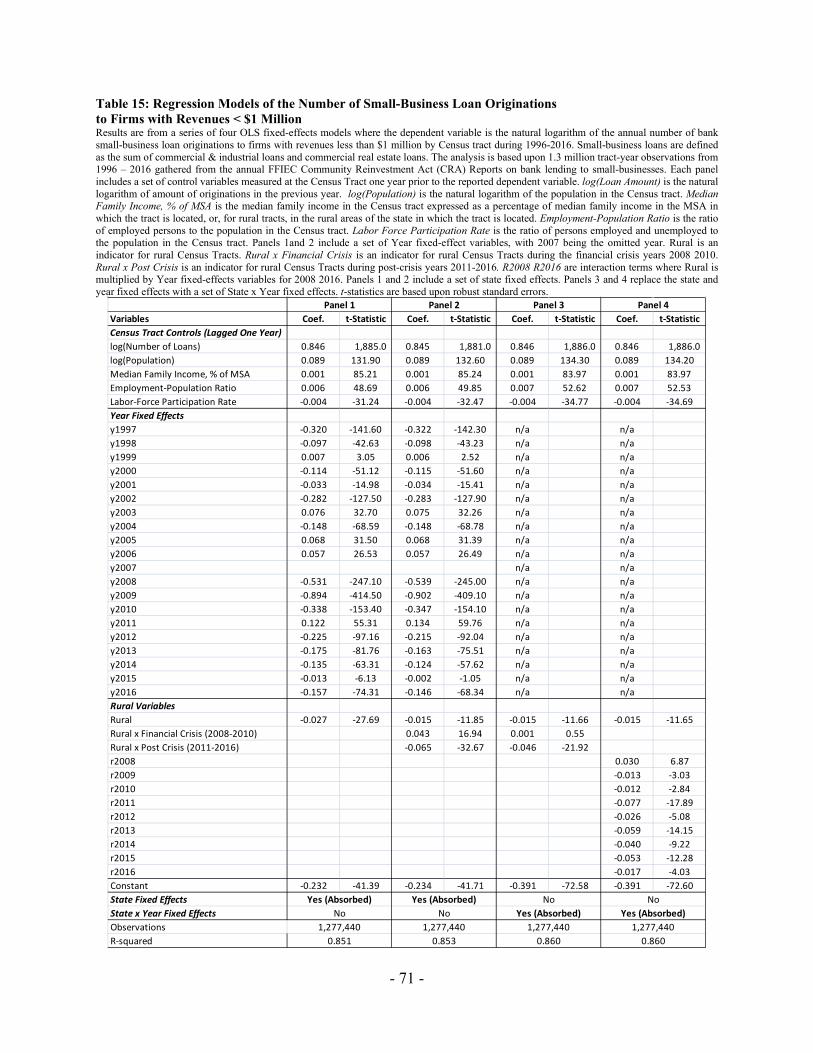
1 Million ................................................................................................................................... - 70 - Table 15: Regression Models of the Number of Small-Business Loan Originations to Firms with Revenues
< $1 Million .............................................................................................................................. - 71 -
- 1 -
Executive Summary
The ability of small businesses to access financing continues to be one of the most
pressing policy issues in the U.S. Given the well-documented role of small businesses in creating
jobs and economic growth, policymakers and regulators must act to ensure that creditworthy
firms and their owners are able to obtain sufficient financing for the businesses to survive
economic downturns and grow during other periods. Without adequate financing, small
businesses will not be able continue their critical contributions to economic growth and
employment.
The data on small-business lending collected by bank regulators to comply with the
Community Reinvestment Act (CRA) of 1977 provides analysts, policymakers, regulators and
the public with information on how much lending each bank is doing in each neighborhood. The
first round of CRA data were released in 1997 and provides information on bank lending during
calendar year 1996, and subsequent rounds have been released each year through 2016. With
information on both the amount and number of loans made by banks in each Census tract, these
data provide incredibly detailed information on the status of bank lending to small businesses in
more than 30,000 neighborhoods. Only banks with assets above a threshold are subject to the
CRA reporting requirements. Although almost 90 percent of banks are exempt, those banks
account for only about 25 percent of total assets.
This report provides an analysis of how lending changed overall and in rural vs. urban
areas before, during, and after the financial crisis of 2008-2010. The analysis shows that rural
firms have poorer access to bank credit than their urban counterparts in terms of both the amount
and number of loans, and that this situation has deteriorated, rather than improved during the
post-crisis years of 2011-2016.
- 2 -
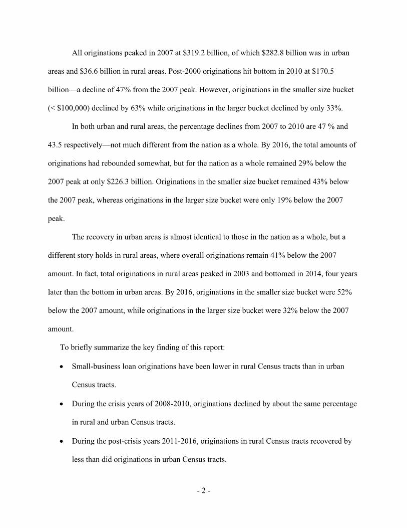
All originations peaked in 2007 at $319.2 billion, of which $282.8 billion was in urban
areas and $36.6 billion in rural areas. Post-2000 originations hit bottom in 2010 at $170.5
billion—a decline of 47% from the 2007 peak. However, originations in the smaller size bucket
(< $100,000) declined by 63% while originations in the larger bucket declined by only 33%.
In both urban and rural areas, the percentage declines from 2007 to 2010 are 47 % and
43.5 respectively—not much different from the nation as a whole. By 2016, the total amounts of
originations had rebounded somewhat, but for the nation as a whole remained 29% below the
2007 peak at only $226.3 billion. Originations in the smaller size bucket remained 43% below
the 2007 peak, whereas originations in the larger size bucket were only 19% below the 2007
peak.
The recovery in urban areas is almost identical to those in the nation as a whole, but a
different story holds in rural areas, where overall originations remain 41% below the 2007
amount. In fact, total originations in rural areas peaked in 2003 and bottomed in 2014, four years
later than the bottom in urban areas. By 2016, originations in the smaller size bucket were 52%
below the 2007 amount, while originations in the larger size bucket were 32% below the 2007
amount.
To briefly summarize the key finding of this report:
• Small-business loan originations have been lower in rural Census tracts than in urban
Census tracts.
• During the crisis years of 2008-2010, originations declined by about the same percentage
in rural and urban Census tracts.
• During the post-crisis years 2011-2016, originations in rural Census tracts recovered by
less than did originations in urban Census tracts.
- 3 -
• These results hold for both the amount and number of small-business loan originations.
The results of this study suggest that inadequate access to financing is an issue that
disproportionately affects rural small businesses. Moreover, the results show that this issue
became even more pronounced during, and, especially, after the financial crisis of 2008-2010.
Future research that may be helpful in formulating policy responses could explore the roles of
differences in the determinants of the supply and demand for loans, including issues like
differences in the availability of business opportunities and differences in the availability of
suitable collateral.
- 4 -
1. Background
During the financial crisis, credit markets in the U.S. virtually froze up. Lax underwriting
standards led to unprecedented levels of nonperforming loans that led bank regulators to close
almost 500 banks during 2009-2012. Cole (2012) documents how these developments affected
bank lending to small businesses, plummeting from 2008 highs by almost 20% during 2009-
2010. Moreover, he also provides evidence that the decline in lending was much greater at large
than at small banks, even though failures were heavily concentrated among small rather than
large banks. Cole (2018) extends this analysis through the recovery years of 2011-2015 and finds
little evidence of a recovery in small-business lending.
The current study extends the works of Cole (2012, 2018) by analyzing FFIEC data at the
census-tract level on bank originations of small-business loans to test whether the decline in
lending documented in those (and other) studies disproportionately impacted small businesses
located in rural areas during the crisis years 2008–2010; and, if so, whether there has been any
sort of recovery during the post-crisis years 2011–2016. The current study also tests whether
banks made fewer loans to small businesses in rural areas before, as well as during and after the
financial crisis. The analysis reveals that banks made fewer loans to rural small businesses
before, during, and after the financial crisis; that rural small businesses were, indeed,
disproportionately hurt during the crisis years relative to urban small businesses, which also were
hurt, but not as severely; and that rural small businesses saw less of a recovery during the post-
crisis years than did their urban counterparts. These findings support efforts by policymakers and
bank regulators to find new policies and regulations that can boost bank small-business lending
in rural areas.
- 5 -
The availability of credit is one of the most fundamental issues facing a small business
and therefore, has received much attention in the academic literature (See, for example, Petersen
and Rajan, 1994; Berger and Udell, 1995; Cole, 1998; Cole, Goldberg and White, 2004; Berger
and Udell, 1995, 1996, 1998a; Cole, 2008, 2009, 2010, 2012, 2018; Cole and Sokolyk, 2016;
Jagtiani and Lemiux, 2016).
Both theory dating back to Shumpeter (1934)1 and more recent empirical research (e.g.,
King and Levine, 1993a, 1993b; Rajan and Zingales, 1998) indicate that capital-constrained
firms grow more slowly, hire fewer workers and make fewer productive investments than firms
utilizing debt in their capital structure. A better understanding of how the bank lending to rural
small businesses fared during the crisis years of 2009 – 2010 and the post-crisis recovery years
of 2011- 2016 should provide policymakers with guidance on how to tailor economic and tax
policies to boost bank lending to small rural firms. These policies will help to increase both
employment and GDP, especially in rural neighborhoods, and reducing disparities in wealth
between rural and urban business owners.
Why is this analysis of importance? According to the U.S. Department of Treasury and
Internal Revenue Service, there were more than 33 million businesses that filed taxes for 2013,
of which 24 million were nonfarm sole proprietorships, 4.3 million were S-corps, 3.5 million
were partnerships and 1.6 million were C-corporations; all but about 10,000 C-corporations were
privately held and the vast majority have annual revenues less than $1 million.2 Small firms are
1 Aghion and Howitt (1988) provide a comprehensive exposition of Schumpeter’s theory of economic growth. 2 See the U.S. Internal Revenue Service statistics for integrated business data at: https://www.irs.gov/uac/soi-tax-stats-integrated-business-data. The year 2013 is used for reference because it was the latest year for which statistics were available at the time this article was written.
vital to the U.S. economy. According to the U.S. Small Business Administration, small
businesses account for 99.9% of all businesses; 48% of private-sector employment; half of all
U.S. private-sector employment and produced 63% of net job growth in the U.S. between 1992
and 2013.3 Therefore, a better understanding of how bank credit to small businesses was affected
by the financial crisis can help policymakers take actions that will lead to more credit, which will
translate into more jobs and faster economic growth.
The current study contributes to the literature on the availability of credit to small
businesses by providing the first rigorous analysis of how bank loan originations to rural small
businesses fared during the crisis and post-crisis years of 2009-2010. New evidence presented in
this study, finding that how rural small businesses were disproportionately impacted relative to
their urban counterparts, suggests that policymakers and regulators need to craft new economic
and tax policies as well as new regulations to encourage banks to boost their lending to small
firms located in rural areas.
2. Literature Review
2.1. Availability of Credit to Small Businesses
The issue of the availability of credit to small businesses has been studied by financial
economists for at least sixty years, dating back at least to Wendt (1946), who examines
availability of loans to small businesses in California. Since then, scores of articles have
addressed this issue.
3 See, “Frequently Asked Questions,” Office of Advocacy, U.S. Small Business Administration (2016) at: https://www.sba.gov/sites/default/files/advocacy/SB-FAQ-2016_WEB.pdf. The SBA defines a small business as “an independent firm with fewer than 500 employees.” We follow that definition in this research.
This review of the literature is limited to the most prominent studies of bank lending
using bank-level loan data that have appeared in the financial economics literature during the
past few years, especially those that use the FFIEC CRA data on small business loan originations
by banks.4 The study most closely related to this one from a methodological viewpoint is Peek
and Rosengren (1998), who examine the impact of bank mergers on small business lending.5
Like us, they examine the change in small business lending (as measured by the ratio of small-
business loans to total assets) by groups of banks subject to different “treatments.” In their study,
the treatment is whether or not the bank was involved in a merger, whereas, in our study, the
treatment is whether or not the borrower is located in a rural census tract. Peek and Rosengren
find that small-business lending of the consolidated bank (post-merger) converges towards the
small-business lending of the pre-merger acquirer rather than that of the pre-merger target.
Ou and Williams (2009) use data from a variety of sources, including the FFIEC Call
Reports, to provide an overview of small business lending by U.S. financial institutions during
the past decade. Using the FFIEC data, they present aggregate statistics from 1995 – 2007 on
small business lending by depository institutions, including a breakdown by institution size and a
discussion on the growing importance of business credit-card loans.
Li (2013) also looks at how the financial crisis affected bank lending, but her focus is on
lending by banks that participated in the Capital Purchase Program (“CPP”). She finds that CPP
4 There also is a related body of work on the availability of credit that relies upon information on the Surveys of Small Business Finances (SSBFs). See, for example, Petersen and Rajan (1994), Berger and Udell (1995), Cole (1998, 2008, 2009, 2010), and Cole, Goldberg and White (2004), Craig and Hardee (2007); Hardee (2007); and Rice and Strahan (2010). 5 There also are a number of other studies that examine how mergers affect small-business lending, including Berger et al. (1998) and Cole and Walraven (1998), but the methodologies in those studies differ from the methodology used here. In addition, many of those studies examine data from the Survey of Terms of Bank Lending rather than from the June Call Reports.
- 8 -
investments boosted bank lending at capital constrained banks by 6.41% per annum. However,
her analysis looks at changes in lending only from 2008Q3 to 2009Q2, so it does not exploit the
panel nature of bank data nor does it capture the full effects of the Great Financial Crisis (GFC).
Cole (2012) uses FFIEC data on the stock of small business loans to examine how small
business lending by banks changed during the GFC years. He finds that, from June 2008 to June
2011, small-business lending declined by $116 billion, or almost 18%, from $659 billion to only
$543 billion; and that small commercial & industrial lending declined by even more, falling by
more than 20% over the same period. Cole also examines lending by banks that did and did not
participate in the CPP. Contrary to Li (2013), who examined all business lending, he finds that
banks participating in the CPP cut small business lending by even more than non-participants.
Finally, Cole documents a strong negative relation between bank size and business lending, and a
strong positive relation between bank capital adequacy and business lending.
Mills and McCarthy (2015) provide an assessment of access to credit by small businesses
during the post-crisis recovery years and how technology may play an important future role.
They argue that structural barriers are at play, such as ongoing consolidation in the banking
industry and high transaction costs of small-dollar-value loans, that impede bank lending to small
businesses. They posit that emerging online lenders may help to mitigate these structural barriers
by providing an alternative supply of small business credit.
Jagtiani and Lemieux (2016) use FFIEC Call Report data on the amount of small business
loans outstanding at depository institutions to document how, since the 1990s, the market share
of small business loans has risen at large banks at the expense of community banks--a trend that
accelerated following onset of the GFC in 2008. They also find that, during the run-up to the
- 9 -
GFC when housing prices were rising rapidly, small businesses increased the use of home equity
lines of credit to fund their operations.
Three recent papers (Bord et al. 2017; Flannery and Lin, 2016; and Jang, 2017) have used
county-level FFIEC data on small business loan originations to analyze the impact of housing
prices on small-business lending during the recent financial crisis.
Bord et al. (2017) use CRA loan-origination data from 2005-2013 to analyze the role of
large banks in propagating financial shocks across the U.S. economy. They find that banks
operating in the counties most severely affected by the decline in housing prices reduced small-
business loan originations even in counties where housing prices were not severely affected by
the crisis. In many cases, these banks ceased to lend in unaffected counties. In contrast, banks not
exposed to loans in severely affected counties expanded their operations. Finally, they report that
their findings persist for years after the initial shock.
Flannery and Lin (2016) use CRA loan-origination data from the pre-crisis period 1996-
2006 analyze how increases in house prices affected small-business lending. They find that the
real estate bubble caused growth not only in real-estate loans, but also in small-business
commercial & industrial loans, even after controlling for local economic conditions.
Jang (2017) uses CRA loan-origination data from 2005-2010 to analyze the effect of the
TARP on the propagation of real estate shocks via geographically diversified U.S. banks.
Employing a difference-in-differences identification strategy, she finds that the amount of TARP
money provided to banks in distressed areas is positively associated with small-business loan
originations in non-distressed areas. She also finds that TARP funds helped recipient banks
return faster to their pre-crisis franchise values.
- 10 -
Rupasingha and Wang (2017) study how access to capital affects the growth rate of U.S.
small businesses. They find that small business growth is positively related to small-business
lending, using county-level CRA data on small-business lending and county-level data on the
number of establishments.
Conroy et al. (2017) examine how changes in small-business lending affects the
subsequent births of establishments. Using annual county-level CRA data on small-business
originations and county-level Census data on establishment births from the Census’ Business
Information Tracking Series they find that the establishment birth rate is higher in counties
where the levels and change in the level of small-business lending are greater. Moreover, they
find that these effects are stronger in rural than in urban counties.
Cole (2018) uses bank-level FFIEC Call Report data on the stock of small-business loans
outstanding as well as bank-level FFIEC CRA loan-origination data on the flow of small-
business loans (i.e., originations) to examine how small-business lending by banks changed
during the GFC crisis years of 2009-2010 as well as during the post-crisis years of 2011-2015.
He finds that bank lending to small businesses remained depressed throughout the post-crisis
years, while total-business lending saw somewhat of a recovery. His analysis also documents
that the declines in small-business lending were significantly greater at large banks than at small
banks, and at banks in worse financial condition than at banks in better financial condition.
2.2. Availability of Credit to Rural Small Businesses
An exhaustive search of the academic literature reveals that there are only a handful of
studies that analyze small-business lending to rural U.S. firms. While there are a number of
studies that look at the availability of credit to rural firms in developing countries, these are of
little relevance to the current study. The closest study to the current one is Laderman and Reid
- 11 -
(2010), who use CRA data on small-business lending to look at lending in low and middle-
income (LMI) areas during the financial crisis. For the entire U.S., they report dramatic declines
in both the number and amount of small-business loan originations from 2007 to 2009. Their
multivariate analysis provides some evidence that lending declined even more in LMI areas than
in middle-income and upper-income areas. However, they do not look directly at lending in rural
versus urban markets.
DeYoung et al. (2012) analyze data on about 18,000 U.S. Small Business Administration
loans made by urban and rural community banks during 1984 – 2001 to investigate how
“ruralness” affects loan default rates. They hypothesize that rural bankers have better
information about their borrowers from closer ties within the rural communities, which should
lead to better underwriting decisions. They find support for this hypothesis in that loans issued
by rural banks and loans issued to rural borrowers default less frequently than comparable urban
loans. They also find that default rates are higher when a banker lends to a borrower who is
located outside of the banker’s geographic market. Their findings provide a possible explanation
for why rural community banks continue to play an important role in lending to small businesses.
Hall and Yeager (2002) analyze financial data from a sample of small rural banks located
in the Midwest to test whether local economic activity affects performance. They examine bank
performance as measured by profitability and asset quality—two of the components of the
CAMELS rating system. They examine local economic activity as measured by unemployment,
employment growth, personal income growth, and per capita income growth at both the county
and state level for the county and state in which their sample banks are located. Surprisingly,
they find that economic activity measured at the state-level, but not county-level, affect the
financial performance of these banks.
- 12 -
3. Data
To conduct this study, the author used data from a number of sources. The primary
source is the FFIEC’s Community Reinvestment Act (CRA) database.6 The CRA was passed
into law in 1977 by Congress (12 U.S.C. 2901) and has been implemented by bank regulators
(see 12 CFR parts 25, 228, 345, and 195). Congress intended that CRA would encourage each
financial institution to take steps to meet the credit needs of borrowers in the localities in which
the institution does business.
In part, the CRA regulations require that financial institutions report annually information
on their lending to small businesses. In particular, they are required to report the numbers and
amounts of business loans originated in amounts less than $100,000, $100,000 - $250,000, and
$250,000 - $1 million. In addition, they must report the number and amount of loans originated
to firms with less than $1 million in revenues. Because these are originations rather than
outstanding portfolio amounts, they represent the flow of new loans to small businesses, whereas
the Call Report data analyzed by Cole (2012, 2018) and others represent the stock of loans to
small business. The FFIEC makes available aggregate loan originations at the granularity of the
state, MSA, county, and Census tract as well as for the country as a whole. Identification by
Census tract enables researchers to merge the loan-origination data with demographic data from
the U.S. Census to identify the urban vs. rural location (and other characteristics) of each census
tract, which are used as proxies for ownership of the firm.
6 The CRA data on small-business loan originations are available for public download from the FFIEC's website at: http://www.ffiec.gov/cra/default.htm.
The CRA provides relief for small banks that are assumed to make business loans only to
small firms; while the threshold for this reporting has changed each year, in general since 2005,
banks with assets less than $1 billion have been exempt from the CRA reporting requirement.
This exemption covers almost 90% of banks by number, but only about 25% by assets.7
Nevertheless, it is an important shortcoming of this source of data; the data are not complete and
do not cover small community banks. The CRA data on small-business loan originations used in
this study span the years 1996 - 2016.
In order to identify lending to rural vs. urban firms, the author obtained Census
demographic (and other) data at the Census-tract level from the FFIEC’s website,8 which were
merged with the Census-tract CRA loan origination data. A Census tract is classified as “rural”
when the Census MSA/MD code is set to a value of 9999, which indicates that the tract falls
outside of a Metropolitan Statistical Area/Metropolitan Division.9 The FFIEC Census data also
provide information at the Census-tract level on a number of variables that can be used to
construct control variables for the analysis. These include population, median family income,
7 These statistics are based upon the author’s calculations using CRA and Call Report data. Similar statistics have been reported by other researchers. 8 These data are available for download at: https://www.ffiec.gov/censusapp.htm. Although there are annual datasets for 1996 through 2016, the 1990 Census data are used for 1996 – 2002, the 2000 Census data are used for 2003-2012, and the 2010 Census data are used for 2013-2016. Hence, there are only three different time-series values over the 21-year period. As described below, the author linearly interpolates data for each non-Census year, using 2016 data from the American Community Survey as the endpoint for 2011-2016. 9 This definition of “rural” includes “Micropolitan Area,” which the OMB defines as a county or county equivalent containing an urban area with a population of at least 10,000 but less than 50,000. A county or county equivalent containing an urban area with a population of 50,000 or more is defined as “Metropolitan Area.” Together, Micropolitan and Metropolitan Areas are known as “Core-Based Statistical Areas” or CBSAs. An alternative definition of rural not used in this study would be areas outside of CBSAs. Yet another definition would be to make use the population in each Census tract that are classified as urban and rural; and classify based upon which is larger. For more information, go to: https://www.census.gov/programs-surveys/metro-micro/about.html
median age, and employment status, among others. The use of data at the Census-tract level
rather than the county or state levels allows more precise matching of lending data to control
variables. The FFIEC Census data are augmented with data from the 2016 five-year estimates
from the Census’ American Community Survey (ACS).10 The author then used the 1990, 2000,
and 2010 Census data and 2016 ACS data to linearly interpolate annual observations for each
control variable.
4. Methodology
4.1 Univariate Tests
In order to provide new evidence on how the financial crisis affected bank lending to
rural small businesses, this study employs both univariate and multivariate tests. First, univariate
tests are used to analyze small-business loan originations in aggregate and by rural vs. urban
census tract. Eight different measures are analyzed; four that measure the dollar amount of small-
business loan originations and four that measure the number of small-business loan originations.
For both number and amount, the four measures are:
• small-business loans originated in amounts less than $100,000;
• small-business loans originated in amounts of $100,000 $250,000;
• small-business loans originated in amounts of $250,000 $1 million; and
• Small-business loans originated to firms with revenues less than $1 million.
4.2 Multivariate Tests
This study also conducts multivariate tests on the data. Statistical techniques that exploit
10 The data and accompanying documentation are available from the Census webpage: https://www.census.gov/acs/www/data/data-tables-and-tools/data-profiles/2016/
the panel nature of the dataset are used to explain eight different measures of small-business
lending--four that measure the dollar amount of small-business loan originations and four that
measure the number of small-business loan originations. More specifically, a variation of the
"difference-in-difference" methodology," which dates back to the seminal study by Ashenfelter
and Card (1985), is used to analyze differences in lending by banks in urban and rural areas.
Imbens and Wooldridge (2007, p. 1) explain the methodology as follows:
"The simplest set-up is one where outcomes are observed for two groups for two
time periods. One of the groups is exposed to a treatment in the second period but
not in the first period. The second group is not exposed to the treatment during
either period. In the case where the same units within a group are observed in
each time period, the average gain in the second (control) group is subtracted
from the average gain in the first (treatment) group. This removes biases in
second-period comparisons between the treatment and control group that could be
the result from permanent differences between those groups, as well as biases
from comparisons over time in the treatment group that could be the result of
trends."
In the current study, two groups—small businesses located in urban vs. rural census
tracts—are exposed to an exogenous shock—the financial crisis. One can then observe whether
the two groups experience differential outcomes in response to the exogenous shock. This is
analogous to a medical experiment that tests whether a particular drug, such as aspirin, has a
differential effect on men and women, allowing for causal inference. (See, e.g., Roncaglioni et
al., 2001.)
Our general model takes the form:
- 16 -
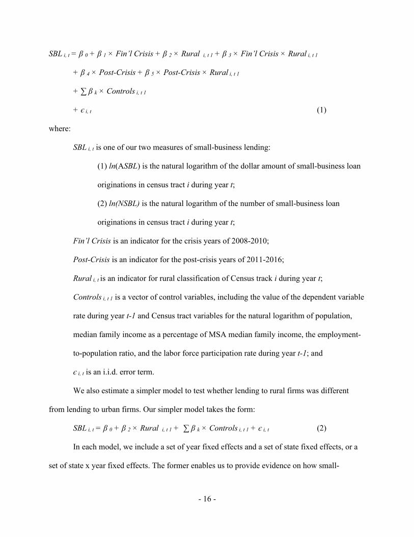
SBL i, t = β 0 + β 1 × Fin’l Crisis + β 2 × Rural i, t 1 + β 3 × Fin’l Crisis × Rural i, t 1
+ β 4 × Post-Crisis + β 5 × Post-Crisis × Rural i, t 1
+ ∑ β k × Controls i, t 1
+ є i, t (1)
where:
SBL i, t is one of our two measures of small-business lending:
(1) ln(ASBL) is the natural logarithm of the dollar amount of small-business loan
originations in census tract i during year t;
(2) ln(NSBL) is the natural logarithm of the number of small-business loan
originations in census tract i during year t;
Fin’l Crisis is an indicator for the crisis years of 2008-2010;
Post-Crisis is an indicator for the post-crisis years of 2011-2016;
Rural i, t is an indicator for rural classification of Census track i during year t;
Controls i, t 1 is a vector of control variables, including the value of the dependent variable
rate during year t-1 and Census tract variables for the natural logarithm of population,
median family income as a percentage of MSA median family income, the employment-
to-population ratio, and the labor force participation rate during year t-1; and
є i, t is an i.i.d. error term.
We also estimate a simpler model to test whether lending to rural firms was different
from lending to urban firms. Our simpler model takes the form:
SBL i, t = β 0 + β 2 × Rural i, t 1 + ∑ β k × Controls i, t 1 + є i, t (2)
In each model, we include a set of year fixed effects and a set of state fixed effects, or a
set of state x year fixed effects. The former enables us to provide evidence on how small-
- 17 -
business lending declined in each year following onset of the financial crisis. The latter enables
us to better control for differences in loan demand across time by state. Although a difference-
in-difference style of model is used, we do not attempt to identify causal relationships with this
analysis.
5. Hypotheses
The primary hypotheses to be tested in this study revolve around the crisis and post-crisis
indicator variables, the treatment variables that indicate rural Census tracts, and the interaction of
the treatment variables with the crisis and post-crisis indicator variables.
H1: Small-business-loan originations throughout the sample period are lower in rural census
tracts than in urban census tracts.
The expectation is that small-business loan originations in rural census tracts are lower than in
urban census tracts because of the challenges faced by businesses in rural areas. This implies that
the expected β 2 coefficient for Rural i, t 1 in equation (2) is negative and statistically significant.
H2A: During the financial-crisis years 2008-2010, small-business-loan originations in rural
census tracts declined by a greater percentage than did originations in urban census tracts
during those years.
Following onset of the financial crisis in 2008, the expectation is that small-business-loan
originations in rural census tracts declined by a greater percentage than did originations in urban
census tracts as banks sought to boost their capital ratios by reducing small-business loans in
general and by reducing loans to borrowers more distant from their headquarters, which are in
- 18 -
urban areas. Bankers would be more loyal to their more credit-worthy customers. This implies
that the coefficient β 3 on Fin’l Crisis × Rural i, t 1 in eq. (1) is negative and statistically
significant.
H2B (alternative to H2A): During the financial crisis years 2008-2010, small-business-loan
originations in rural census tracts declined by less than did originations in urban census tracts
during those years.
As an alternative to H2A, the expectation is that, following onset of the financial crisis in 2008,
small-business-loan originations in rural census tracts declined by less than did originations in
urban census tracts as bankers sought to raise their capital ratios by reducing originations to less
creditworthy borrowers. DeYoung et al. (2012) provide evidence that rural small businesses are
less likely to default than are their urban counterparts. This implies that the expected coefficient
β 3 on Crisis × Rural i, t 1 in eq. (1) is positive and significantly different from zero.
H3A: During the post-crisis years 2011-2016, small-business loan originations in rural census
tracts recovered by a greater percentage than did originations in urban census tracts during
those years.
The expectation is that small-business loan originations, in general, recovered post crisis (β 4 >
0), but we also expect that originations in rural census tracts recovered by more than originations
in urban census tracts, as bankers sought to expand credit to their more creditworthy customers.
This implies that the coefficient β 5 on Post-Crisis × Rural i, t 1 is positive and statistically
significant.
- 19 -
H3B (alternative to H3A): During the post-crisis years 2011-2016, small-business loan
originations in rural census tracts recovered by less than did originations in urban census
tracts during those years.
As an alternative to H3A, the expectation is that small-business-loan originations recovered post
crisis (β 4 > 0), but that originations in rural census tracts recovered by less than originations in
urban census tracts, as bankers returned to funding their less creditworthy borrowers.
This implies that the coefficient β 5 on Post-Crisis × Rural i, t 1 is negative and statistically
significant.
6. Results
6.1. Univariate Results
6.1.1. Amounts of Originations by Loan Size
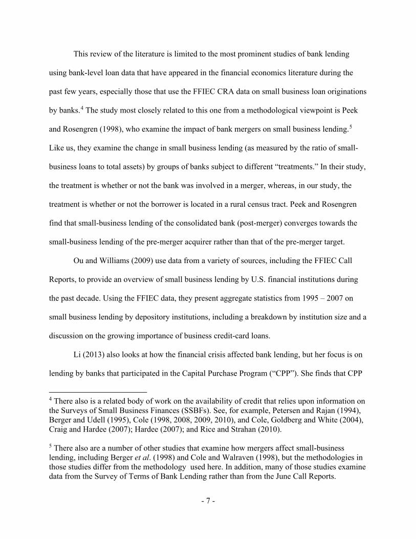
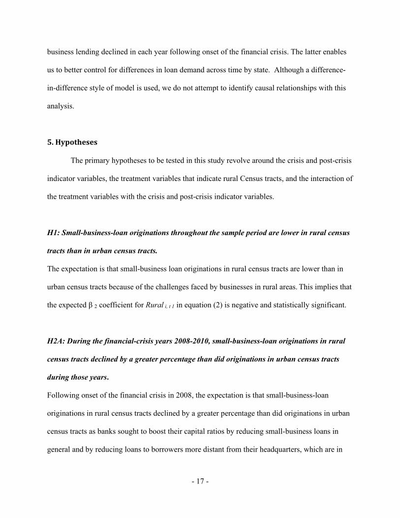
Figures 1 – 2 show the aggregate amounts of small-business-loan originations by year for
two size buckets of loans: less than $100,000, and $100,000 to $1 million. This information also
appears in tabular form in Table 1. Aggregate originations peaked in 2007 at $319 billion, of
which $282 billion was in urban areas and $37 billion in rural areas. Post-2000, aggregate
originations hit bottom in 2010 at $170 billion—a decline of 47% from the 2007 peak. However,
originations in the smaller size bucket (< $100,000) declined by 63% while originations in the
larger bucket declined by only 33%.
- 20 -
Figure 1: Figure 2: SBL Originations, 1996-2016 SBL Originations, 1996-2016 Originated in Amounts < $100,000 Originated in Amounts $100,000 $1 Million Aggregate Dollar Amounts in Urban vs. Rural Areas Aggregate Dollar Amounts in Urban vs. Rural Areas
0
5
10
15
20
25
30
35
0
20
40
60
80
100
120
140
160
180
200
1996 2000 2004 2008 2012 2016
$ Billions
Urban Rural
0
5
10
15
20
25
30
35
0
20
40
60
80
100
120
140
160
180
200
1996 2000 2004 2008 2012 2016
$ Billions
Urban Rural
Figure 3: Figure 4: SBL Originations per Capita, 1996-2016 SBL Originations per Capita, 1996-2016 Originated in Amounts < $100,000 Originated in Amounts $100,000 $1 Million Average Dollar Amounts per Capita in Urban vs. Rural Areas Average Dollar Amounts per Capita in Urban vs. Rural Areas
0
50
100
150
200
250
300
350
400
0
100
200
300
400
500
600
1996 2000 2004 2008 2012 2016
Dollars per Capita
Urban Rural
0
100
200
300
400
500
600
0100200300400500600700800900
1,000
1996 2000 2004 2008 2012 2016
Dollars per Capital
Urban Rural
In both urban and rural areas, the percentage declines from 2007 to 2010 are almost
identical to the nation as a whole. By 2016, the aggregate originations had rebounded somewhat,
but for the nation as a whole remained 29% below the 2007 peak at only $226 billion.
Originations in the smaller size bucket remained 43% below the 2007 peak, whereas originations
in the larger size bucket were only 18% below the 2007 peak.
- 21 -
The recovery in urban areas is almost identical to those in the nation as a whole, but a
different story holds in rural areas, where overall originations remain 41% below the 2007 peak.
In fact, total originations in rural areas bottomed in 2014, four years later than the bottom in
urban areas. Rural originations in the smaller size bucket were 52% below the 2007 peak, while
rural originations in the larger size bucket were 32% below the 2007 peak. In summary,
originations in both urban and rural areas dropped by more than 40% during the crisis years;
from 2010 to 2016, originations have rebounded noticeably in urban areas, but there has been
almost no such recovery in rural areas. Overall, the univariate statistics indicate that originations
in both urban and rural areas suffered about equally during the crisis years of 2008 – 2010, but
that there has been much less of a recovery in rural areas. These results support only hypothesis
H3B: during the post-crisis years of 2011 – 2016, originations in rural areas recovered by less
than did originations in urban areas.
The geographic boundaries of MSAs are often altered a few years after a decennial
census.11 Changes in classification from rural to urban following the 2010 Census may account
for some or all of the observed decrease the total lending amounts for rural areas, creating
patterns like those shown in Figures 1 and 2 above.
To address this issue, loan amounts in each Census tract can be scaled by the population
in each Census tract. The average of loan amounts per capita should provide a more meaningful
comparison of trends and a more direct univariate comparison of rural to urban lending levels.12
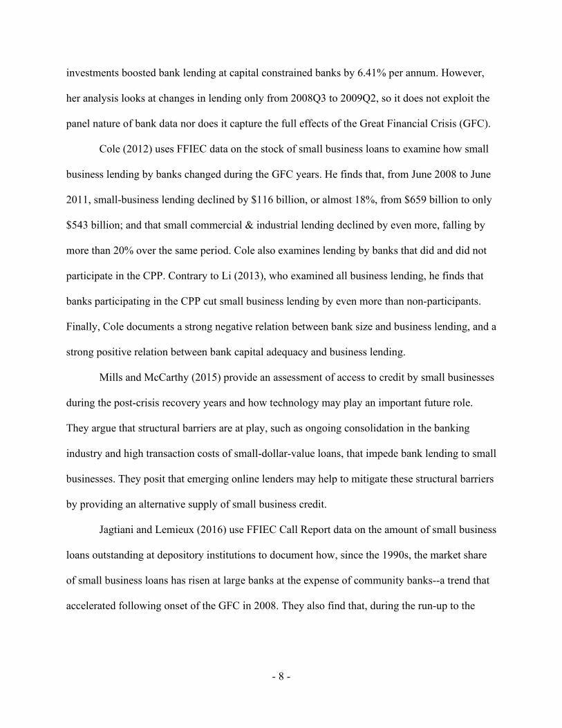
Figures 3 – 4 show the average amounts of small-business-loan originations per capita by year
for two size buckets of loans: less than $100,000, and $100,000 to $1 million. This information
11 For details, see information at the website of the U.S. Census: https://www.census.gov/programs-surveys/acs/geography-acs/concepts-definitions.html. 12 The author is grateful to peer reviewers and SBA staff for suggesting this line of analysis.
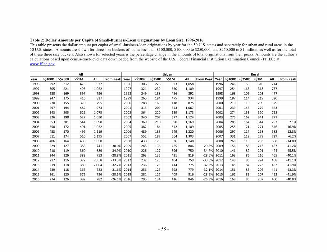
also appears in tabular form in Table 2. Both Figures 3 and 4 show a less pronounced rebound in
lending to firms in urban areas relative to firms in rural areas than do Figures 1 and 2, indicating
that changes in MSA boundaries may account for some of the differences shown in Figures 1
and 2.
Average originations per capita peaked nationally in 2007 at $1,195; for urban areas in
2007 at $1,303; and for rural areas in 2004 at only $793. Post-2000, average originations per
capita nationally hit bottom in 2010 at $689—a decline of 42% from the 2007 peak. However,
originations in the smaller size bucket (< $100,000) declined by 59% from their 2007 to the 2010
trough while originations in the larger bucket declined by only 30% from peak to trough.
By 2016, average originations per capita nationally had recovered somewhat, but
remained 35% below their peak; originations in urban areas also had recovered to 35% below
their 2007 peak, but originations in rural areas remained near crisis lows, down 42% from their
2004 peak.
In summary, originations per capita in both urban and rural areas dropped by more than
40% during the crisis years; from 2010 to 2016, originations per capita in urban areas recovered
somewhat, but there has been almost no such recovery in rural areas. Overall, the univariate
statistics indicate that originations in both urban and rural areas suffered about equally during the
crisis years of 2008 – 2010, but that there has been less of a recovery in rural areas. These results
support only hypothesis H3B: during the post-crisis years of 2011 – 2016, originations in rural
areas recovered by less than did originations in urban areas.
6.1.2. Amounts of Originations to Firms with Revenues less than $1 Million
In addition to collecting information on small-business-loan originations by size of the
loan, the FFIEC also collects information on small-business-loan originations to firms with
- 23 -
revenues less than $1 million. Because mid-size and even large firms may borrow in amount less
than $1 million, information on firms with revenues less than $1 million is more indicative of
lending to truly small businesses.
Figure 5: Figure 6: SBL Originations, 1996-2016 SBL Originations, 1996-2016 Originated to Firms with Revenues < $1 Million Originated to Firms with Revenues < $1 Million Aggregate Dollar Amounts in Urban vs. Rural Areas Average Dollar Amounts per Capita in Urban vs. Rural Areas
0
5
10
15
20
25
30
0
20
40
60
80
100
120
140
1996 2000 2004 2008 2012 2016
$ Billions
Urban Rural
0
100
200
300
400
500
600
0
100
200
300
400
500
600
1996 2000 2004 2008 2012 2016
Dollars per Capita
Urban Rural
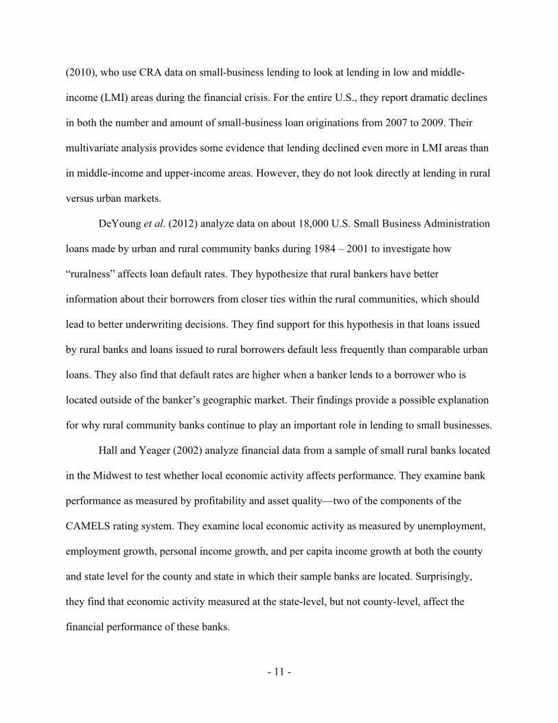
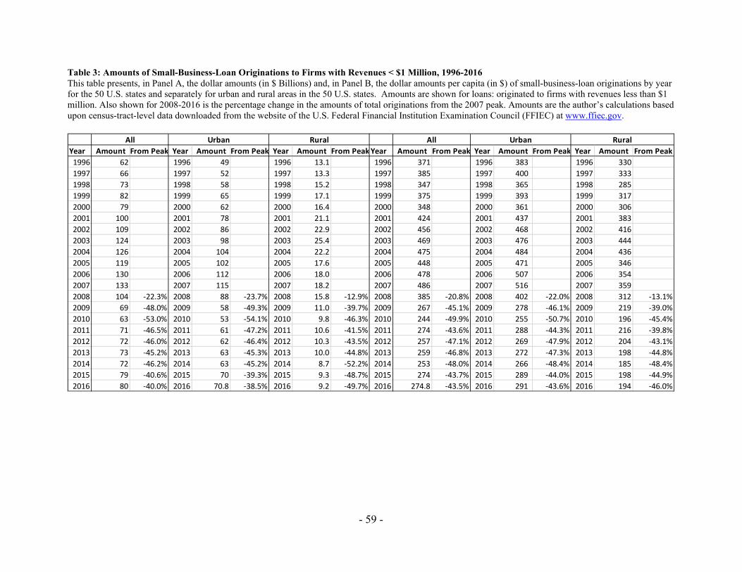
Figures 5 and 6 show the aggregate dollar amounts (in $ millions) and average dollar
amounts per capita, respectively, of small-business-loan originations to firms with revenues less
than $1 million in urban and rural areas. This information also appears in tabular form in
Table 3.
As was true for aggregate amounts by loan size, the aggregate loan amounts to firms with
revenues less than $1 million peaked during 2007. Originations nationally peaked at $133
billion, of which $115 billion were in urban areas and $18 billion were in rural areas. Overall,
originations hit bottom in 2010 at $62.6 billion—a decline of 53%. Originations in urban areas
also hit bottom in 2010 down 53%. However, originations in rural areas did not bottom until
2014 down 52%.
By 2016, the aggregate amounts of originations to firms with revenues less than $1
million had rebounded somewhat, but for the nation as a whole remained 40% below the 2007
- 24 -
peak at only $80 billion. In 2016, originations in urban areas were 38% below the peak, but, in
rural areas, originations were still 50% below the peak. These results provide support for H3B,
that during the post-crisis years of 2011 – 2016, originations in rural areas recovered by less than
did originations in urban areas.
As shown in Panel B of Table 3 and Figure 6, the average amount of originations per
capita nationally also peaked in 2007 at $486 and in urban areas at $516; however, the peak rural
areas occurred in 2003 at $444. Nationally and in urban areas, originations per capita hit bottom
in 2010 at $244 and $$255, respectively; but in rural areas, originations per capita hit bottom in
2014 at $185. Since the bottoms, originations per capita have recovered to $291 in urban areas
but only to $194 in rural areas.
In summary, the results for average originations to firms with revenues less than $1
million provide support for hypothesis H3B: during the post-crisis years of 2011 – 2016,
originations in rural areas recovered by less than did originations in urban areas.
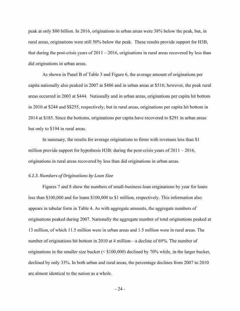
6.1.3. Numbers of Originations by Loan Size
Figures 7 and 8 show the numbers of small-business-loan originations by year for loans
less than $100,000 and for loans $100,000 to $1 million, respectively. This information also
appears in tabular form in Table 4. As with aggregate amounts, the aggregate numbers of
originations peaked during 2007. Nationally the aggregate number of total originations peaked at
13 million, of which 11.5 million were in urban areas and 1.5 million were in rural areas. The
number of originations hit bottom in 2010 at 4 million—a decline of 69%. The number of
originations in the smaller size bucket (< $100,000) declined by 70% while, in the larger bucket,
declined by only 33%. In both urban and rural areas, the percentage declines from 2007 to 2010
are almost identical to the nation as a whole.
- 25 -
Figure 7: Figure 8: SBL Originations 1996-2016 SBL Originations 1996-2016 Originated in Amounts < $100,000 Originated in Amounts $100,000 $1 Million Aggregate Number of Loans in Urban vs. Rural Areas Aggregate Number of Loans in Urban vs. Rural Areas
0.0
0.5
1.0
1.5
2.0
0
2
4
6
8
10
12
1996 2000 2004 2008 2012 2016
Millions
UrbanRural
0.00
0.02
0.04
0.06
0.08
0.10
0.0
0.1
0.2
0.3
0.4
0.5
1996 2000 2004 2008 2012 2016
Millions
UrbanRural
Figure 9: Figure 10: SBL Originations 1996-2016 SBL Originations 1996-2016 Originated in Amounts < $100,000 Originated in Amounts $100,000 $1 Million Average Number of Loans per Capita in Urban vs. Rural Areas Average Number of Loans per Capita in Urban vs. Rural Areas
0.00
0.01
0.02
0.03
0.04
0.05
0.00
0.01
0.02
0.03
0.04
0.05
1996 2000 2004 2008 2012 2016
Num
ber o
f Loa
ns p
er C
apita
UrbanRural
0.000
0.001
0.002
0.003
0.000
0.001
0.002
0.003
1996 2000 2004 2008 2012 2016
Num
ber o
f Loa
ns p
er C
apita
s
UrbanRural
By 2016, the numbers of originations had rebounded somewhat, but, nationally, remained
54% below the 2007 peak at only 6.0 billion. Originations in the smaller size bucket remained
55% below the 2007 peak, whereas originations in the larger size bucket were only 19% below
the 2007 peak. The recovery in urban areas is almost identical to those at the national level, but
once again a different story holds in rural areas, where the aggregate number of originations
remains 63% below the 2007 peak.
- 26 -
In summary, the number of originations in both urban and rural areas dropped by almost
70% during the peak crisis years. Since 2010, the rebound in number of originations has been
much stronger in urban relative to rural areas. Overall, these results provide support for H3B,
that, during the post-crisis years of 2011 – 2016, originations in rural areas recovered by less
than did originations in urban areas.
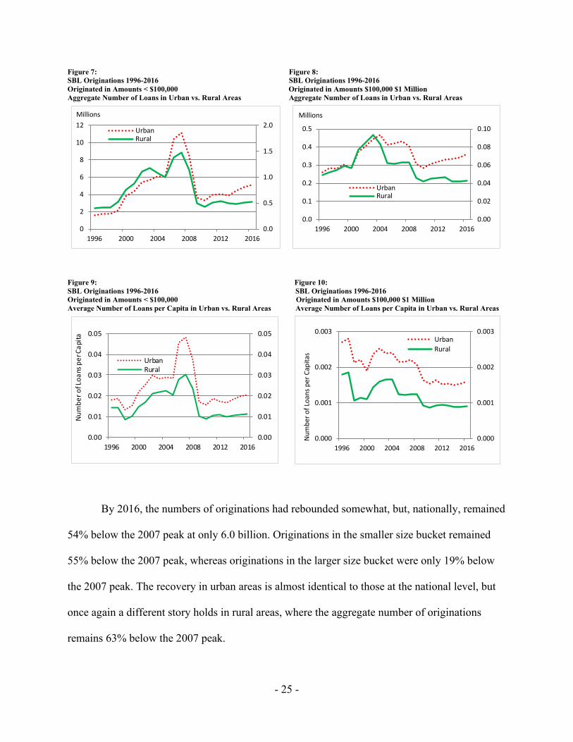
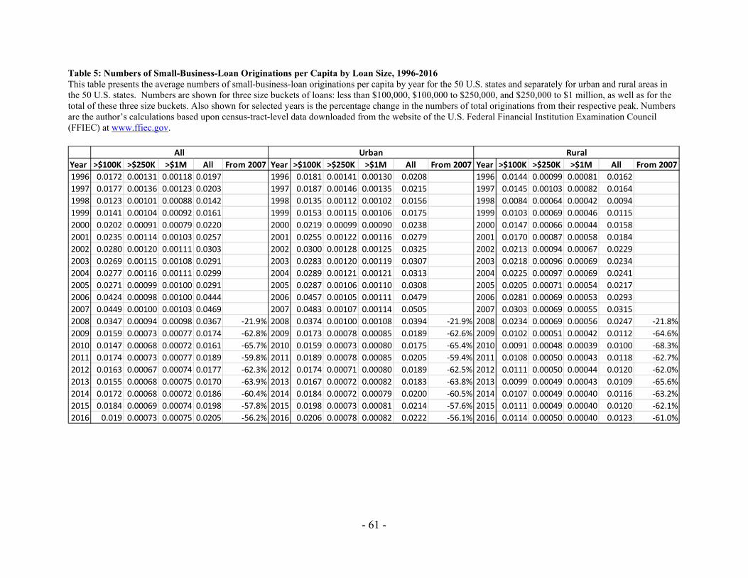
Figures 9 and 10 show the average numbers of small-business-loan originations per
capita by year for loans less than $100,000 and for loans $100,000 to $1 million, respectively.
This information also appears in tabular form in Table 5. The average numbers of loans per
capita peaked during 2007 at 0.047 nationally; at 0.051 in urban areas; and at 0.032 in rural
areas. The number of originations per capita hit bottom nationally in 2010 at 0.016—a decline of
66%. Similar percentage declines were seen in both urban and rural areas.
By 2016, the average numbers of originations per capita had rebounded somewhat, but,
for the nation as a whole, remained 56% below the 2007 peak at only 0.021. The recovery in
urban areas is almost identical to those nationally; but in rural areas, the average number of
originations per capita remained at 61% below the 2007 peak.
In summary, the average number of originations per capita in both urban and rural areas
dropped by almost 70% during the peak crisis years. Since 2010, the rebound in number of
originations has been somewhat stronger in urban relative to rural areas. Overall, these results
provide support for H3B, that, during the post-crisis years of 2011 – 2016, originations in rural
areas recovered by less than did originations in urban areas.
- 27 -
Figure 11: Figure 12: SBL Originations 1996-2016 SBL Originations 1996-2016 Firms with Revenues < $1 Million Firms with Revenues < $1 Million Number of Loans in Urban vs. Rural Areas Number of Loans per Capita in Urban vs. Rural Areas
0.0
0.2
0.4
0.6
0.8
1.0
0
1
2
3
4
5
1996 2000 2004 2008 2012 2016
Millions of Loans
UrbanRural
0.000
0.005
0.010
0.015
0.020
0.025
0.000
0.005
0.010
0.015
0.020
0.025
1996 2000 2004 2008 2012 2016
Num
ber o
f Loa
ns p
er C
apita
UrbanRural
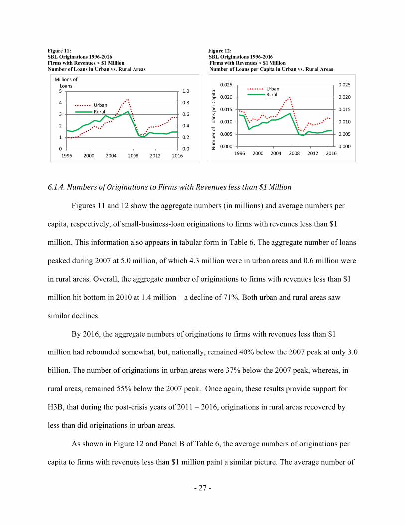
6.1.4. Numbers of Originations to Firms with Revenues less than $1 Million
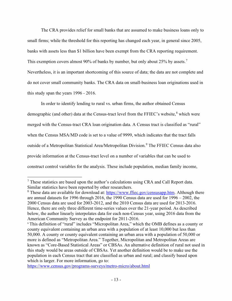
Figures 11 and 12 show the aggregate numbers (in millions) and average numbers per
capita, respectively, of small-business-loan originations to firms with revenues less than $1
million. This information also appears in tabular form in Table 6. The aggregate number of loans
peaked during 2007 at 5.0 million, of which 4.3 million were in urban areas and 0.6 million were
in rural areas. Overall, the aggregate number of originations to firms with revenues less than $1
million hit bottom in 2010 at 1.4 million—a decline of 71%. Both urban and rural areas saw
similar declines.
By 2016, the aggregate numbers of originations to firms with revenues less than $1
million had rebounded somewhat, but, nationally, remained 40% below the 2007 peak at only 3.0
billion. The number of originations in urban areas were 37% below the 2007 peak, whereas, in
rural areas, remained 55% below the 2007 peak. Once again, these results provide support for
H3B, that during the post-crisis years of 2011 – 2016, originations in rural areas recovered by
less than did originations in urban areas.
As shown in Figure 12 and Panel B of Table 6, the average numbers of originations per
capita to firms with revenues less than $1 million paint a similar picture. The average number of
- 28 -
originations per capita peaked during 2007 at 0.019 nationally; at 0.020 in urban areas and at
0.013 in rural areas. This metric hit bottom in 2010 down 68% nationally. Both urban and rural
areas saw similar declines.
By 2016, the average numbers of originations per capita to firms with revenues less than
$1 million had rebounded somewhat, but, both nationally and in urban areas, remained 43%
below the 2007 peak. In rural areas, this metric remained 51% below the 2007 peak. Once again,
these results provide support for H3B, that during the post-crisis years of 2011 – 2016,
originations in rural areas recovered by less than did originations in urban areas.
6.2. Multivariate Results
In addition to the univariate evidence presented above, this section presents multivariate
evidence based on panel-data regression models analyzing the amounts and numbers of small-
business-loan originations. While the univariate results highlight differences in small business
lending between Census tracts in urban and rural areas, they do not control for important
differences in the characteristics of urban versus rural firms. One important difference is
population. Rural areas may have fewer loans simply because they have fewer people. Other
important differences are age, income, and employment.
Four models are estimated for four measures of the amounts and four measures of the
number of small-business-loan-originations: amounts and numbers of originations in amounts
less than $1 million, amounts and numbers of originations in amounts less than $100,000,
amounts and numbers of originations in amounts greater than $250,000 and less than $1 million,
and amounts and numbers of originations to firms with revenues less than $1 million. For each of
the eight dependent variables, the first model (shown in Panel 1) corresponds to eq. (2), and
- 29 -
includes only the control variables, a set of Year fixed effects (with 2007 being the omitted
“baseline” year), and an indicator for rural Census tracts.13 The control variables are from the
most recently available Census (1990, 2000 or 2010) and include the natural logarithm of tract
population, the median family income as a percentage of median MSA income, the ratio of
employment to population, and the labor force participation rate (the sum of employment and
unemployment divided by population). This model provides for a clean test of hypothesis H1.
The second model (shown in Panel 2) augments the first model with an interaction of Rural and
Fin’l Crisis plus an interaction of Rural and Post Crisis. These interaction terms provide a means
for testing hypotheses H2 and H3. The third model (shown in Panel 3) is similar to the second
model but replaces the year fixed effects and state fixed effects with a set of 2,000 State × Year
fixed effects, i.e. one indicator for each state and year pair (50 states times 20 years). State and
state-year fixed effects are “absorbed” so there are no coefficients for these variables.14
The fourth model (shown in Panel 4) is similar to the third model but replaces the interaction of
Rural and Fin’l Crisis and the interaction of Rural and Post Crisis with a set of indicators for
rural Census tracts in each year during 2008 – 2016.
6.2.1. Descriptive Statistics
Table 7 presents descriptive statistics for the Census-tract dependent and control
variables that are included in the multivariate analysis. During 1996-2016, the Census-tract
average amounts of originations in the small, middle, and large size buckets were $1.130 million,
$558 thousand and $1.645 million, respectively. The average amount of originations to firms
with revenues less than $1 million was $1.383 million. The average numbers of originations in
13 The first three models also include a set of state fixed effects, but these variables are not shown in the tables. 14 The averages of all explanatory variables are calculated for each state-year pair and these are subtracted from the values of the explanatory variables, leaving deviations from the means.
- 30 -
the small, medium, and large size buckets were 86.3, 3.2, and 3.1, respectively. The average
number of originations to firms with revenues less than $1 million was 38.8. When one compares
the average amounts and numbers of originations between urban and rural tracts, one finds that
the averages in rural tracts are significantly small. For the average amounts in the small, medium,
and large size buckets, rural originations are 67%, 74%, and 53% as large as in urban areas. For
the average amount to firms with revenues less than $1 million, rural originations are 81% as
large as in urban areas. For the average numbers in the small, medium, and large size buckets,
rural originations are 62%, 77%, and 56% as large as in urban areas. For the average number to
firms with revenues less than $1 million, rural originations are 74% as large as in urban areas.
Table 7 also presents descriptive statistics for five tract-level control variables. The average
population was 4,264 but was 4,372 in urban areas and 3,827 in rural areas. The average median
family income as a percentage of MSA median family income was 100.35 but was 100.66 in
urban areas and 99.10 in rural areas. The average median family age was 35.6 but was 35.2 in
urban areas and 37.1 in rural areas. The average employment-population ratio was 59.3 but was
60.2 in urban areas and 55.7 in rural areas. Finally, the average labor-force participation rate was
63.7, but was 64.6 in urban areas and 59.8 in rural areas. Each of these differences in means is
statistically significant.
6.2.2. Multivariate Regression Models of the Amount of Small-Business-Loan Originations
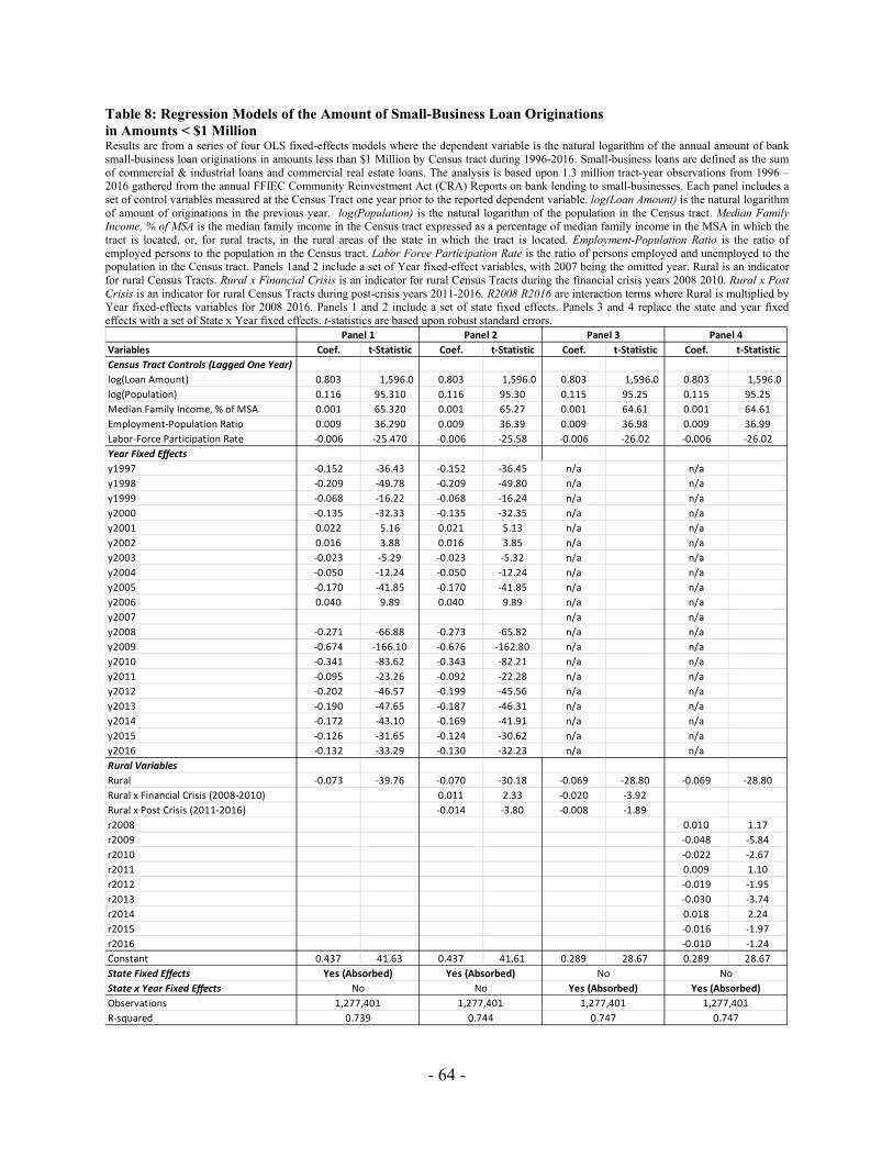
Table 8 presents the results from a series of regression models where the dependent
variable is the natural logarithm of the amounts of small-business-loan originations in amounts
less than $1 million. The adjusted R2 indicates that the model explains approximately 75% of the
variability in the data. Each of the year fixed effects for 2008 – 2016 is estimated with great
precision, as indicated by the extremely large t-statistics shown in the first three models.
- 31 -
Figure 13: Figure 14: Amounts of SBL Originations in Amounts < $1 Million Amounts of SBL Originations in Amounts < $1 Million Percentage Declines from 2007 Percentage Differences in Rural Areas during 2008-2016 2008-2016 vs. Urban Areas in 2007
-24
-49
-29
-9
-18 -17 -16-12 -12
-60
-50
-40
-30
-20
-10
0
2008 2009 2010 2011 2012 2013 2014 2015 2016
Percent
-5.7
-11.4
-8.9
-5.8
-8.6-9.6
-4.8
-8.3-7.7
-12
-10
-8
-6
-4
-2
0
2008 2009 2010 2011 2012 2013 2014 2015 2016
Percent
As shown in Figure 13, these coefficients indicate that, relative to the omitted year of 2007, the
amounts of originations dropped by 24% in 2008, 49% in 2009, and 29% in 2010.15 In 2011,
originations were down by only 9% relative to 2007, but then deteriorated again during 2012-
2014 (down 18%, 17%, and 16%, respectively). During 2015 and 2016, originations remained
more than ten percent below those in 2007. Over this same period, total business loans rose by
more than 46%.16 So, almost a decade after the onset of the financial crisis, the amount of small-
business-loan originations in amounts less than $1 million remains significantly below pre-crisis
levels, even as total business lending has risen by almost half.
The key variables of interest in Table 8 are the indicator for rural Census tracts and the
crisis and year interactions with this indicator. Panel 1 includes only an indicator for rural Census
tracts, providing a clean test of H1. The highly significant coefficient on Rural indicates that, on
average, originations in rural areas were exp (-0.073) – 1 = 7.0% lower than originations in urban
areas during the sample period 1996 – 2016. This result strongly supports H1 that originations
15 In a semi-logarithmic model like this one, one must transform the coefficient to obtain the implied percentage change in the dependent variable. The transformation is to exponentiate the coefficient and then subtract one. In Excel, this calculation is “exp(coefficient) – 1.” See Halvorsen and Palmquist (1980). 16 This figure is based upon the author’s calculations using data reported in the FDIC’s Quarterly Banking Profiles.
- 32 -
throughout the sample period are lower in rural areas than in urban areas. Qualitatively similar
results are obtained when the state fixed effects are replaced by State × Year fixed effects.
In Panel 2, indicator variables for rural Census tracts during the financial crisis years of
2008-2010 and during the post-crisis years of 2011-2016 are added to the specification in Panel
1. The highly significant coefficient on Rural declines only slightly, from 0.073 to 0.070. The
0.011 coefficient on Rural × Fin’l Crisis is statistically significant at the 0.05 level and indicates
that, during the financial crisis years, lending in rural areas fell by 1.1 percentage points less than
in urban areas. The0.014 coefficient on Rural × Post Crisis is statistically significant at the 0.01
level and indicates that, during the post crisis years, lending in rural areas fell by 1.4 percentage
points more than in urban areas.
In Panel 3, the specification in Panel 2 is changed by replacing the year fixed effects and
state fixed effects with a set of State ×Year fixed effects. This better controls for changes in local
economic conditions, as it controls for unobserved state-level heterogeneity in each year. The
results in Panel 3 show almost no effect on the coefficient on Rural but show that the sign on the
coefficient of Rural × Fin’l Crisis changes from positive to negative, and the coefficient is
significant at better than the 0.01 level. The interaction of Rural and post-crisis remains negative
and significant, but only at the 0.10 level. These results provide support for H2A that small-
business loan originations during the crisis years declined by more at rural than at urban firms,
and for H3B that small-business loans during the post-crisis years recovered by less at rural than
at urban firms.
In Panel 4, the specification in Panel 3 is altered by replacing the two rural crisis
interaction variables with a set of nine Year × Rural indicators. This model sheds additional light
upon changes in rural lending within the two crisis periods. The coefficients for 2009 and 2010
- 33 -
are negative and significant at better than the 0.01 level, while the coefficients for 2008 is
positive but not significantly different from zero. Taken together, these results support H2A that,
during the financial crisis years, originations in rural census tracts declined by a greater
percentage than did originations in urban census tracts. During the post crisis years, four of the
coefficient are negative (2012, 2013, 2015, and 2016) and two are positive (2011 and 2014). The
negative coefficient for 2013 is significant at better than the 0.01 level while the negative
coefficient for 2015 is significant at the 0.05 level and the negative coefficient for 2012 is
significant at the 0.06 level. Taken together, these results provide weak evidence in favor of H3B
that originations in rural census tracts recovered by less than did originations in urban census
tracts during the post-crisis years 2011 – 2016.
To calculate the percentage difference for originations in rural areas by year relative to
originations to urban firms during the omitted year of 2007, one adds the average effect during
the pre-crisis period with the Year × Rural interaction effect. As shown in Figure 14, the
interaction terms indicate that, relative to 2007, originations in rural areas were 5%11% lower
during 2008 – 2016.
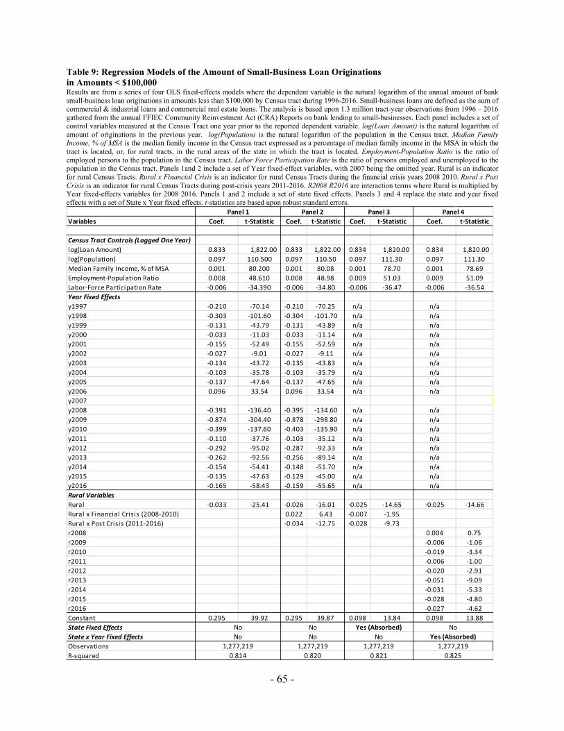
Table 9 presents the results from a series of regression models where the dependent
variable is the natural logarithm of the amount of small-business-loan originations in amounts
less than $100,000. This is the smallest of the three size buckets and hence, is better
representative of lending to truly small businesses. Data from the Federal Reserve Board’s 2003
Survey of Small Businesses indicate that the average small business in the U.S. had only about
$60,000 in total assets (Cole and Sokolyk, 2016).
As shown in Figure 15, the year coefficients indicate that, relative to the omitted year of
2007, the amounts of originations in amounts less than $100,000 dropped by 33% in 2008, 58%
- 34 -
in 2009, and 33% in 2010. In 2011, originations were down by only 10% relative to 2007, but
then deteriorated again during 2012 – 2013 (down 25% and 22%, respectively). During 2016,
originations remained 15% below those in 2007.
Figure 15: Figure 16: Amounts of SBL Originations in Amounts < $100,000 Amounts of SBL Originations in Amounts < $100,000 Percentage Declines from 2007 Percentage Differences in Rural Areas during 2008-2016 2008-2016 vs. Urban Areas in 2007
-33
-58
-33
-10
-25 -23
-14 -12 -15
-70
-60
-50
-40
-30
-20
-10
0
2008 2009 2010 2011 2012 2013 2014 2015 2016
Percent
-2.0-3.1
-4.4
-3.0
-4.4
-7.4
-5.5 -5.2 -5.1
-8
-7
-6
-5
-4
-3
-2
-1
0
2008 2009 2010 2011 2012 2013 2014 2015 2016
Percent
In Panel 1, the highly significant coefficient on Rural indicates that, on average,
originations in rural areas were exp (-0.033) – 1 = 3.2% lower than originations in urban areas
during the sample period 1996 – 2016. This result strongly supports H1 that originations
throughout the sample period are lower in rural areas than in urban areas. Qualitatively similar
results are obtained when the State and Year fixed effects are replaced by State × Year fixed
effects.
In Panel 2, indicator variables for rural Census tracts during the financial crisis years of
2008-2010 and during the post-crisis years of 2011-2016 are added to the specification in Panel
1. The highly significant coefficient on Rural declines slightly, from 0.033 to 0.026. The 0.022
coefficient on Rural × Fin’l Crisis is statistically significant at the 0.05 level and indicates that,
during the financial crisis years, lending in rural areas fell by 2.2 percentage points less than in
urban areas. The0.034 coefficient on Rural × Post Crisis is statistically significant at the 0.01
- 35 -
level and indicates that, during the post crisis years, lending in rural areas fell by 3.3 percentage
points more than in urban areas.
In Panel 3, the specification in Panel 2 is changed by replacing the year fixed effects and
state fixed effects with a set of state x year fixed effects. The results in Panel 3 show almost no
effect on the coefficient on Rural but show that the sign on the coefficient of Rural × Fin’l Crisis
changes from positive to negative, and the coefficient is significant at better than the 0.06 level.
The interaction of Rural and post-crisis remains negative and significant at better than the 0.01
level. These results provide support for H2A that small-business loan originations during the
crisis years declined by more at rural than at urban firms, and for H3B that small-business loans
during the post-crisis years recovered by less at rural than at urban firms.
In Panel 4, the specification in Panel 3 is altered by replacing the two rural crisis
interaction variables with a set of nine Year × Rural indicators. The coefficients for 2009 and
2010 are negative and, for 2010, significant at better than the 0.01 level, while the coefficient for
2008 is positive but not significantly different from zero. Taken together, these results support
H2A that, during the financial crisis years, originations in rural census tracts declined by a
greater percentage than did originations in urban census tracts. During the post crisis years, each
of the six coefficients is negative and five are significant at the 0.05 level or better. Taken
together, these results provide strong evidence in favor of H3B that originations in rural census
tracts recovered by less than did originations in urban census tracts during the post-crisis years
2011 – 2016.
As shown in Figure 16, the interaction terms indicate that originations in rural areas
during 2008 – 2016 were 2% 7% lower than in urban areas during 2007.
- 36 -
Table 10 presents the results from a series of regression models where the dependent
variable is the natural logarithm of the amounts of small-business-loan originations in the largest
size bucket—amounts greater than $250,000 and less than $1 million.
Figure 17: Figure 18: Amounts of SBL Originations in Amounts $250,000-$1 Million Amounts of SBL Originations in Amounts $250,000-$1 Million Percentage Declines from 2007 Percentage Differences in Rural vs. Urban Areas 2008-2016 2008-2016
-15
-49-41
-24 -21 -24
-34-28
-24
-60
-50
-40
-30
-20
-10
0
2008 2009 2010 2011 2012 2013 2014 2015 2016
Percent
-32
-39-36 -36
-39
-34
-25
-32-36
-45-40-35-30-25-20-15-10
-50
2008 2009 2010 2011 2012 2013 2014 2015 2016
Percent
As shown in Figure 17, the year coefficients indicate that, relative to the omitted year of
2007, the amounts of originations dropped by 15% in 2008, 49% in 2009, and 41% in 2010. In
2011-2016, originations were down by 20% 35% relative to 2007. During 2016, originations
remained more than twenty percent below those in 2007.
In Panel 1, the highly significant coefficient on Rural indicates that, on average,
originations in rural areas were exp (-0.470) – 1 = 37.5% lower than originations in urban areas
during the sample period 1996 – 2016. This result strongly supports H1 that originations
throughout the sample period are lower in rural areas than in urban areas. Qualitatively similar
results are obtained when the State and Year fixed effects are replaced by State × Year fixed
effects.
In Panel 2, indicator variables for rural Census tracts during the financial crisis years of
2008-2010 and during the post-crisis years of 2011-2016 are added to the specification in Panel
- 37 -
1. The highly significant coefficient on Rural rises slightly, from0.470 to0.499. The 0.083
coefficient on Rural × Fin’l Crisis is statistically significant at the 0.05 level and indicates that,
during the financial crisis years, lending in rural areas fell by 8.7 percentage points less than in
urban areas. The 0.058 coefficient on Rural × Post Crisis is statistically significant at the 0.01
level and indicates that, during the post crisis years, lending in rural areas fell by 5.9 percentage
points less than in urban areas.
In Panel 3, the specification in Panel 2 is changed by replacing the year fixed effects and
state fixed effects with a set of State × Year fixed effects. The results in Panel 3 show almost no
effect on the coefficient on Rural but show that the coefficient of Rural × Fin’l Crisis declines in
magnitude from 0.083 to 0.037 but remains significant at better than the 0.05 level. The
interaction of Rural and post-crisis remains positive and significant at better than the 0.101 level.
These results provide support for H2B that small-business loan originations during the crisis
years declined by less at rural than at urban firms, and support for H3A that small-business loans
during the post-crisis years recovered by more at rural than at urban firms.
In Panel 4, the specification in Panel 3 is altered by replacing the two rural crisis
interaction variables with a set of nine Year × Rural indicators. The coefficients for 2008, 2009,
and 2010 are positive and, for 2008, significant at better than the 0.05 level. Taken together,
these results support H2B that, during the financial crisis years, originations in rural census tracts
declined by a smaller percentage than did originations in urban census tracts. During the post
crisis years, each of the six coefficients is positive and three are significant at the 0.10 level or
better. Taken together, these results provide evidence in favor of H3A that originations in rural
census tracts recovered by more than did originations in urban census tracts during the post-crisis
years 2011 – 2016.
- 38 -
As shown in Figure 18, the interaction terms indicate that originations in rural areas
during 2008 – 2016 were 25% 39% lower than in urban areas during 2007.
Table 11 presents the results from a series of regression models where the dependent
variable is the natural logarithm of the amount of small-business-loan originations the firms with
revenues less than $1 million. Many researchers consider this measure the most representative of
lending to truly small businesses. Data from the Federal Reserve Board’s 2003 Survey of Small
Businesses indicate that the average small business in the U.S. had about $600,000 in revenues
(Cole and Sokolyk, 2016).
Figure 19: Figure 20: Amounts in SBL Originations to Firms Amounts in SBL Originations to Firms with with Revenues <$ Million Revenues <$1 Million Percentage Declines from 2007 Percentage Differences in Rural Areas during 2008-2016 2008-2016 vs. Urban Areas in 2007
-33
-52
-36
-11
-26-21 -21
-11
-18
-60
-50
-40
-30
-20
-10
0
2008 2009 2010 2011 2012 2013 2014 2015 2016
Percent
-6
-10-9 -9
-13
-10-9 -9
-11
-14
-12
-10
-8
-6
-4
-2
0
2008 2009 2010 2011 2012 2013 2014 2015 2016
Percent
As shown in Figure 19, the year coefficients indicate that, relative to the omitted year of
2007, the amounts of originations dropped by 33% in 2008, 52% in 2009, and 36% in 2010. In
2011, originations were down by only 12% relative to 2007, but then deteriorated again during
2012 – 2014 (down 25%, 21%, and 22%, respectively). During 2016, originations remained 17%
below those in 2007. These are very similar to the results reported for the smallest size bucket of
originations shown in Table 7 and Figure 9.
- 39 -
In Panel 1, the highly significant coefficient on Rural indicates that, on average,
originations in rural areas were exp (-0.078) – 1 = 7.5% lower than originations in urban areas
during the sample period 1996 – 2016. This result strongly supports H1 that originations
throughout the sample period are lower in rural areas than in urban areas. Qualitatively similar
results are obtained when the state and year fixed effects are replaced by state x year fixed
effects.
In Panel 2, indicator variables for rural Census tracts during the financial crisis years of
2008-2010 and during the post-crisis years of 2011-2016 are added to the specification in Panel
1. The highly significant coefficient on Rural declines slightly, from 0.078 to 0.065. The 0.022
coefficient on Rural × Fin’l Crisis is statistically significant at the 0.01 level and indicates that
during the financial crisis years, lending in rural areas fell by 2.2 percentage points less than in
urban areas. The0.059 coefficient on Rural × Post Crisis is statistically significant at the 0.01
level and indicates that, during the post crisis years, lending in rural areas fell by 5.7 percentage
points more than in urban areas.
In Panel 3, the specification in Panel 2 is changed by replacing the year fixed effects and
state fixed effects with a set of State × Year fixed effects. The results in Panel 3 show almost no
effect on the coefficient on Rural but show that the sign on the coefficient of Rural x Fin’l Crisis
changes from positive to negative, and the coefficient is significant at better than the 0.05 level.
The coefficient of Rural × Post Crisis remains negative and significant at better than the 0.01
level. These results provide support for H2A that small-business loan originations during the
crisis years declined by more at rural than at urban firms, and for H3B that small-business loans
during the post-crisis years recovered by less at rural than at urban firms.
- 40 -
In Panel 4, the specification in Panel 3 is altered by replacing the two rural crisis
interaction variables with a set of nine Year × Rural indicators. The coefficients for 2009 and
2010 are negative and significant at better than the 0.10 level, while the coefficient for 2008 is
positive but not significantly different from zero. Taken together, these results support H2A that,
during the financial crisis years, originations in rural census tracts declined by a greater
percentage than did originations in urban census tracts. During the post crisis years, each of the
six coefficients is negative and significant at the 0.05 level or better. Taken together, these results
provide strong evidence in favor of H3B that originations in rural census tracts recovered by less
than did originations in urban census tracts during the post-crisis years 2011 – 2016. As shown in
Figure 20, the interaction terms indicate that originations in rural areas during 2008 – 2016 were
6% 13% lower than in urban areas during 2007.
6.2.4. Multivariate Regression Models of the Number of Small-Business-Loan Originations
Table 12 presents the results from a series of regression models where the dependent
variable is the natural logarithm of the number of small-business-loan originations in amounts
less than $1 million. The adjusted R2 in each of these models is greater than 0.90.
As shown in Figure 21, the year coefficients indicate that, relative to the omitted year of
2007, the numbers of originations dropped by 29% in 2008, 60% in 2009, and 25% in 2010. In
2011, originations were essentially even with 2007, but then deteriorated again during 2012 –
2013 (down 14% and 19%, respectively). During 2014 – 2016, the number of originations
remained about eight percent below those in 2007.
In Panel 1, the highly significant coefficient on Rural indicates that, on average,
originations in rural areas were exp (-0.025) – 1 = 2.4% lower than originations in urban areas
- 41 -
during the sample period 1996 – 2016. This result supports H1 that originations throughout the
sample period are lower in rural areas than in urban areas. Qualitatively similar results are
obtained when the state and year fixed effects are replaced by State × Year fixed effects.
Figure 21: Figure 22: Numbers of SBL Originations in Amounts < $1 Million Numbers of SBL Originations in Amounts < $1 Million Percentage Declines from 2007 Percentage Differences in Rural Areas during 2008-2016 2008-2016 vs. Urban Areas in 2007
-29
-60
-25
0
-13-19
-6 -8 -10
-70
-60
-50
-40
-30
-20
-10
0
2008 2009 2010 2011 2012 2013 2014 2015 2016
Percent
-2
-4-3 -3
2
-8
-3
-5
-3
-10
-8
-6
-4
-2
0
2
4
2008 2009 2010 2011 2012 2013 2014 2015 2016
Percent
In Panel 2, indicator variables for rural Census tracts during the financial crisis years of
2008-2010 and during the post-crisis years of 2011-2016 are added to the specification in Panel
1. The highly significant coefficient on Rural declines slightly, from 0.025 to 0.021. The 0.010
coefficient on Rural × Fin’l Crisis is statistically significant at the 0.01 level and indicates that
during the financial crisis years, lending in rural areas fell by 1.0 percentage points less than in
urban areas. The0.019 coefficient on Rural × Post Crisis is statistically significant at the 0.01
level and indicates that, during the post crisis years, lending in rural areas fell by 1.9 percentage
points more than in urban areas.
In Panel 3, the specification in Panel 2 is changed by replacing the Year fixed effects and
State fixed effects with a set of State × Year fixed effects. The results in Panel 3 show a small
reduction in the coefficient on Rural but show that the sign on the coefficient of Rural × Fin’l
Crisis changes from positive to negative, and the coefficient is significant at better than the 0.01
level. The coefficient of Rural × Post Crisis remains negative and significant at better than the
- 42 -
0.01 level. These results provide support for H2A that small-business loan originations during
the crisis years declined by more at rural than at urban firms, and for H3B that small-business
loans during the post-crisis years recovered by less at rural than at urban firms.
In Panel 4, the specification in Panel 3 is altered by replacing the two rural crisis
interaction variables with a set of nine Year × Rural indicators. The coefficients for 2009 and
2010 are negative and significant at better than the 0.01 level, while the coefficient for 2008 is
positive but not significantly different from zero. Taken together, these results support H2A that,
during the financial crisis years, originations in rural census tracts declined by a greater
percentage than did originations in urban census tracts. During the post crisis years, five of the
six coefficients are negative and significant at the 0.01 level or better, while R2012 is positive
and significant at the 0.01 level. Taken together, these results still provide strong evidence in
favor of H3B that originations in rural census tracts recovered by less than did originations in
urban census tracts during the post-crisis years 2011 – 2016.
As shown in Figure 22, the interaction terms indicate that originations in rural areas
during 2008 – 2016 were 2% 8% lower than in urban areas during 2007, except for 2012 when
they were 2% higher.
Table 11 presents the results from a series of regression models where the dependent
variable is the natural logarithm of the number of small-business-loan originations in amounts
less than $100,000. In general, these results are very similar to those in Table 10 because the
number of loans in this size bucket account for the vast majority of all small-business loans, as
shown in Figure 4 above.
In Panel 1, the highly significant coefficient on Rural indicates that, on average,
originations in rural areas were exp (-0.026) – 1 = 2.5% lower than originations in urban areas
- 43 -
during the sample period 1996 – 2016. This result supports H1 that originations throughout the
sample period are lower in rural areas than in urban areas. Qualitatively similar results are
obtained when the state and year fixed effects are replaced by state x year fixed effects.
In Panel 2, indicator variables for rural Census tracts during the financial crisis years of
2008-2010 and during the post-crisis years of 2011-2016 are added to the specification in Panel
1. The highly significant coefficient on Rural declines slightly, from 0.026 to 0.021. The 0.009
coefficient on Rural × Fin’l Crisis is statistically significant at the 0.01 level and indicates that
during the financial crisis years, lending in rural areas fell by 0.9 percentage points less than in
urban areas. The 0.021 coefficients on Rural × Post Crisis is statistically significant at the 0.01
level and indicates that, during the post crisis years, lending in rural areas fell by 2.0 percentage
points more than in urban areas.
In Panel 3, the specification in Panel 2 is changed by replacing the year fixed effects and
state fixed effects with a set of state x year fixed effects. The results in Panel 3 show a small
reduction in the coefficient on Rural but show that the sign on the coefficient of Rural × Fin’l
Crisis changes from positive to negative, and the coefficient is significant at better than the 0.01
level. The coefficient of Rural × Post Crisis remains negative and significant at better than the
0.01 level. These results provide support for H2A that small-business loan originations during
the crisis years declined by more at rural than at urban firms, and for H3B that small-business
loans during the post-crisis years recovered by less at rural than at urban firms.
In Panel 4, the specification in Panel 3 is altered by replacing the two rural crisis
interaction variables with a set of nine Year × Rural indicators. The coefficients for 2009 and
2010 are negative and significant at better than the 0.01 level, while the coefficient for 2008 is
positive but not significantly different from zero. Taken together, these results support H2A that,
- 44 -
during the financial crisis years, originations in rural census tracts declined by a greater
percentage than did originations in urban census tracts. During the post crisis years, five of the
six coefficients are negative and significant at the 0.01 level or better, while R2012 is positive
and significant at the 0.01 level. Taken together, these results still provide strong evidence in
favor of H3B that originations in rural census tracts recovered by less than did originations in
urban census tracts during the post-crisis years 2011 – 2016.
Table 14 presents the results from a series of regression models where the dependent
variable is the natural logarithm of the number of small-business-loan originations in amounts
greater than $250,000 and less than $1 million. The adjusted R2s for these models, in the range of
0.60, are much lower than those for the smallest size bucket (< $100,000) shown in Table 11.
Figure 23: Figure 24: Numbers of SBL Originations in Amounts $250,000 $1 Million Numbers of SBL Originations in Amounts $250,000 $1 Million Percentage Declines from 2007 Percentage Differences in Rural Areas during 2008-2016 2008-2016 vs. Urban Areas in 2007
-6
-5
-6
-8 -8
-6
-5
-7-8
-10
-9
-8
-7
-6
-5
-4
-3
-2
-1
0
2008 2009 2010 2011 2012 2013 2014 2015 2016
Percent
As shown in Figure 23, the year coefficients indicate that, relative to the omitted year of
2007, the numbers of originations dropped by 6% in 2008, 18% in 2009, and 11% in 2010. These
declines are only about one-third as large as those for the number of originations in amounts less
than $100,000, but still are both statistically and economically significant. During 2011 – 2012,
originations were down only 4%, but then deteriorated somewhat during 2013 – 2014 (down 5%
- 45 -
and 9%, respectively). During 2015 – 2016, the number of originations remained about five
percent below those in 2007.
In Panel 1, the highly significant coefficient on Rural indicates that, on average,
originations in rural areas were exp (-0.079) – 1 = 7.6% lower than originations in urban areas
during the sample period 1996 – 2016. This result supports H1 that originations throughout the
sample period are lower in rural areas than in urban areas. Qualitatively similar results are
obtained when the state and year fixed effects are replaced by state x year fixed effects.
In Panel 2, indicator variables for rural Census tracts during the financial crisis years of
2008-2010 and during the post-crisis years of 2011-2016 are added to the specification in Panel
1. The highly significant coefficient on Rural increases slightly, from 0.079 to 0.088. The 0.038
coefficient on Rural × Fin’l Crisis is statistically significant at the 0.01 level and indicates that,
during the financial crisis years, lending in rural areas fell by 3.9 percentage points less than in
urban areas. The 0.013 coefficient on Rural × Post Crisis is statistically significant at the 0.01
level and indicates that, during the post crisis years, lending in rural areas fell by 1.3 percentage
points less than in urban areas.
In Panel 3, the specification in Panel 2 is changed by replacing the year fixed effects and
state fixed effects with a set of State × Year fixed effects. The results in Panel 3 show small
changes in the coefficients, but the coefficients on both Rural × Fin’l Crisis and Rural × Post
Crisis remain positive and significant at better than the 0.01 level. These results provide support
for H2B that small-business loan originations during the crisis years declined by less at rural than
at urban firms, and for H3A that small-business loans during the post-crisis years recovered by
more at rural than at urban firms.
- 46 -
In Panel 4, the specification in Panel 3 is altered by replacing the two rural crisis
interaction variables with a set of nine Year × Rural indicators. The coefficients for 2008, 2009,
and 2010 are positive and significant at better than the 0.01 level. Taken together, these results
support H2B that during the financial crisis years, originations in rural census tracts declined by a
smaller percentage than did originations in urban census tracts. During the post crisis years, each
of the six coefficients are negative and three are significant at the 0.05 level or better. Taken
together, these results provide strong evidence in favor of H3A that originations in rural census
tracts recovered by more than did originations in urban census tracts during the post-crisis years
2011 – 2016.
As shown in Figure 24, the interaction terms indicate that originations in rural areas
during 2008 – 2016 were 5% 8% lower than in urban areas during 2007.
Table 15 presents the results from a series of regression models where the dependent
variable is the natural logarithm of the number of small-business-loan originations to firms with
revenues less than $1 million. The adjusted R2s for these models, in the range of 0.85, are similar
to those for the smallest size bucket (< $100,000) shown in Table 9.
As shown in Figure 25, the year coefficients indicate that, relative to the omitted year of
2007, the numbers of originations dropped by 42% in 2008, 59% in 2009, and 29% in 2010.
These declines are very similar to those for the number of originations in amounts less than
$100,000. During 2011, originations rebounded strongly, up 14% relative to 2007, but then
deteriorated during 2012 – 2014 (down 19%, 15%, and 12%, respectively). During 2015,
originations were flat relative to 2007, but turned south again during 2016, down 14% from 2007
levels.
- 47 -
Figure 25: Figure 26: Numbers of SBL Originations to Firms with Revenues $1 Million Numbers of SBL Originations to Firms with Revenues $1 Million Percentage Declines from 2007 Percentage Differences in Rural Areas during 2008-2016 2008-2016 vs. Urban Areas in 2007
-42
-59
-29
14
-19 -15 -12
-0.2
-14
-70-60-50-40-30-20-10
01020
2008 2009 2010 2011 2012 2013 2014 2015 2016
Percent
1.6
-2.7 -2.7
-8.9
-4.0
-7.2
-5.3-6.6
-3.2
-10.0
-8.0
-6.0
-4.0
-2.0
0.0
2.0
4.0
2008 2009 2010 2011 2012 2013 2014 2015 2016
Percent
In Panel 1, the significant coefficient on Rural indicates that, on average, originations in
rural areas were exp (-0.027) – 1 = 2.6% lower than originations in urban areas during the
sample period 1996 – 2016. This result supports H1 that originations throughout the sample
period are lower in rural areas than in urban areas. Qualitatively similar results are obtained
when the state and year fixed effects are replaced by state x year fixed effects.
In Panel 2, indicator variables for rural Census tracts during the financial crisis years of
2008-2010 and during the post-crisis years of 2011-2016 are added to the specification in
Panel 1. The highly significant coefficient on Rural declines from 0.026 to 0.015. The 0.043
coefficient on Rural × Fin’l Crisis is statistically significant at the 0.01 level and indicates that
during the financial crisis years, lending in rural areas fell by 4.4 percentage points less than in
urban areas. The0.065 coefficient on Rural × Post Crisis is statistically significant at the 0.01
level and indicates that during the post crisis years, lending in rural areas fell by 6.3 percentage
points more than in urban areas.
In Panel 3, the specification in Panel 2 is changed by replacing the year fixed effects and
state fixed effects with a set of State × Year fixed effects. The results in Panel 3 show no change
in the coefficient on Rural but show that the on the coefficient of Rural × Fin’l Crisis drops from
- 48 -
0.043 to a statistically insignificant 0.001. The coefficient of Rural × Post Crisis remains
negative and significant at better than the 0.01 level. These results provide no support for H2A or
H2B regarding small-business loan originations during the crisis years, but strongly support H3B
that small-business loans during the post-crisis years recovered by less at rural than at urban
firms.
In Panel 4, the specification in Panel 3 is altered by replacing the two rural crisis
interaction variables with a set of nine Year × Rural indicators. The coefficient for 2008 is
positive and significant at better than the 0.01 level, while the coefficients for both 2009 and
2010 are negative and significant at better than the 0.01 level. Taken together, these results
provide at least weak support H2A that, during the financial crisis years, originations in rural
census tracts declined by a greater percentage than did originations in urban census tracts.
During the post crisis years, each of the six coefficients are negative and significant at the 0.01
level or better. Taken together, these results still provide strong evidence in favor of H3B that
originations in rural census tracts recovered by less than did originations in urban census tracts
during the post-crisis years 2011 – 2016.
As shown in Figure 26, the interaction terms indicate that originations in rural areas
during 2008 – 2016 were 2% 9% lower than in urban areas during 2007, with the exception of
2008 when they were 2% higher.
6.2.4. Robustness Tests
The models above include the natural logarithm of population as a control variable. Some
researchers, such as Conroy et al. (2017), prefer to scale the loan data by population rather than
include population as a control variable. When the analysis above is repeated using this
alternative specification, the results are qualitatively unchanged.
- 49 -
The preferred model above includes year x state fixed effects. When the analysis is
repeated using county fixed effects, the results are qualitatively unchanged.
The t-statistics in the models above are based upon robust standard errors. When the
analysis is repeated using standard errors clustered at the county or Census tract, the results are
qualitatively unchanged.
Figure 27: Summary of Findings from Multivariate Regression Analysis Regarding Small-Business-Loan Originations during 1996 – 2016
Amounts <$1M
Amounts <$100K
Amounts $250K-$1M
Amounts Revenues
<$1M
Numbers <$1M
Numbers <$100K
Numbers $250K-$1M
Numbers Revenues
<$1MH1 Small-business loan originations throughout
the sample period are lower in rural census tracts than in urban census tracts.
Yes. Yes. Yes. Yes. Yes. Yes. Yes. Yes.
H2A During the crisis years 2008-2010, small-business loan originations in rural census tracts declined by a greater percentage than did originations in urban census tracts during those years.
Yes. Yes. No. Yes. Yes. Yes. No. No.
H2B During the crisis years 2008-2010, small-business loan originations in rural census tracts declined by no more than did originations in urban census tracts during those years.
No. No. Yes. No. No. No. Yes. No.
H3A During the post-crisis years 2011-2016, small-business loan originations in rural census tracts recovered by a greater percentage than did originations in urban census tracts during those years.
No. No. Yes. No. No. No. Yes. No.
H3B During the post-crisis years 2011-2016, small-business loan originations in rural census tracts recovered by less than did originations in urban census tracts during those years.
Yes. Yes. No. Yes. Yes. Yes. No. Yes.
Dependent Variable
Hypothesis
6.2.5. Summary of Findings from Multivariate Regression Analysis
Figure 27 summarizes the findings from the multivariate regression analysis presented in
Tables 613 and discussed above. Each of the eight models provides support for H1, which
hypothesized that small-business-loan originations throughout the sample period are lower in
rural census tracts than in urban census tracts. The average differentials are not only statistically
significant, they also are economically significant. For the largest size bucket of loans, the
amount of originations in rural areas was lower by 37 percent per year, while the number of
originations in rural areas was lower by eight percent per year.
- 50 -
Six of the eight models provide support for H2A, which hypothesized that, during the
crisis years 2008-2010, small-business loan originations in rural census tracts declined by a
greater percentage than did originations in urban census tracts during those years. The same six
models provide support for H3B, which hypothesized that, during the post-crisis years 2011-
2016, small-business-loan originations in rural census tracts recovered by less than did
originations in urban census tracts during those years.
The two models that failed to support both H2A and H3B were the models where the
dependent variables were the numbers and the amounts of originations in amounts of $250,000
$1 Million. This is the largest of the three size buckets of small-business loans, and many in the
past have argued that such loans are more representative of mid-market firms rather than of
small-businesses.
The finding here certainly suggests that there are fundamental differences in these larger
loans and the loans in the smallest size bucket as well as loans originated to firms with revenues
less than $1 million. Bankers and industry analysts have argued that there are large fixed-amount
origination costs that have increased in the Dodd-Frank era, making smaller loans increasing less
profitable, or even unprofitable. The results reported here suggest that banks reporting the CRA
data analyzed in this study have disproportionately reduced their rural lending in the form of
smaller loans in favor of larger loans.
- 51 -
7. Summary and Conclusions
As the first rigorous analysis based upon tract-level loan origination data on how the
financial crisis and post-crisis recovery impacted bank lending to rural U.S. small businesses, the
current study provides both academics and policymakers with new insights into how the
financial crisis and post-crisis recovery have affected the availability of credit to small rural
firms as compared with urban small firms. It also details how to tailor macroeconomic policies,
regulations, and taxes to help rural small businesses to obtain needed credit. This is critically
important because theory suggests that credit-constrained firms will be smaller, less likely to hire
new employees, and less likely to make new long-term investments that could improve economic
growth. Policies that help these firms improve their capitalization should lead to higher growth in
both employment and output (GDP).
The analysis reveals that small-business-loan originations collapsed during the financial
crisis in both urban and rural areas, but, during post-crisis years, rural originations have
recovered to a much lesser extent than have urban originations.
The multivariate analysis reveals strong differences in the recovery by size of loan. Post-
crisis, originations of loans in amount > $250,000 - $1 million have been stronger in rural areas
than in urban areas, while originations of smaller loans have been much weaker in rural areas
relative to urban areas.
From a policy perspective, the results lead to several recommendations. The most
obvious is for regulators and policymakers to incentivize banks to originate more small-business
loans in rural and other less-served areas, such as low-income and minority areas. One such
option being discussed is to count such loans as “community development loans” when
evaluating a bank’s CRA rating. This would seem to be an especially promising avenue for
- 52 -
incentivizing the “big four” banks with at least $1 trillion in assets that control almost half of
industry assets. Another option would be to expand both the number and amount of loans in rural
areas that are guaranteed by U.S. Small Business Administration loans. Such guarantees reduce
potential losses from making loans and should increase the supply of credit in favored areas.
Another policy would be to reduce the underwriting burden on banks that make small-
business loans in terms of documentation for exam classification purposes. Many in the banking
industry have blamed increased underwriting burden from the Dodd-Frank Act as one reason for
the sluggish bank lending to small businesses (see Decker et al. (2016), and Bordo and Duca,
(2018)). Such “low-doc” loans were used with some success during the 1991-1993 credit crisis.
Yet another policy would be to encourage the growth of small-business lending by
nonbank lenders. Recent changes to small-business loan limits on the almost 6,000 U.S. credit
unions are one such action. A credit union had been limited to investing 12.25 percent of its total
assets in business loans to members, and many credit unions had reached this limit; the proposed
change increases this limit to 27.5 percent of assets. Credit union lending to small businesses has
more than doubled from 2008 to 2016, from $30 billion to $60 billion, while bank lending to
small businesses over the same period has declined by almost $100 billion.
Finally, policymakers and regulators should be careful not to strangle the nascent
FinTech industry, which is growing its small-business lending portfolio at triple-digit rates.
There are calls to more strictly regulate firms in this industry, which may prevent these firms
from serving as a viable alternative to commercial bank lenders.
Certainly, additional research is called for on this important issue. The current study is
limited by the use of aggregate data, albeit at a very granular level. Such data to not allow one to
provide evidence on what types of banks have disproportionately reduced their lending in rural
- 53 -
areas. Future research should look at what types of banks are responsible for the results
documented here. For example, is this result attributable to a decline in rural lending by the
largest banks, which have become much larger since the onset of the financial crisis? The current
analysis also is limited by the coverage of the CRA origination data. Only banks with more than
$1 billion in assets are required to file the CRA reports that are the source of the data. Are
community banks and credit unions stepping in to fill the void in rural lending left by the banks
required to report CRA data? This would be a fruitful avenue for future research.
- 54 -
References
Ashenfelter, O., Card, D. (1985). Using the longitudinal structure of earnings to estimate the effect of training programs. Review of Economics and Statistics 67, 648-660. Aghion, P., Howitt, P. (1988). Endogenous growth theory. Vol. 1, 1st ed. The MIT Press. Berger, A., Saunders, A., Scalise, J., Udell, G. (1998). The effects of bank mergers and acquisitions on small business lending. Journal of Financial Economics 50, 187-229 Berger, A., Udell, G. (1995). Relationship lending and lines of credit in small firm finance. Journal of Business 68, 351-381. Berger, A., Udell, G. (1996). Universal banking and the future of small business lending. In: Saunders, A., Walter, I. (Eds.), Financial System Design: The Case for Universal Banking. Irwin, Burr Ridge, IL, pp. 559 – 627. Berger, A., Udell, G. (1998a). The economics of small business finance: The roles of private equity and debt markets in the financial growth cycle. Journal of Banking & Finance 22 (6-8), 613–673. Berger, A., Udell, G. (1998b). The institutional memory hypothesis and the pro-cyclicality of bank lending behavior, Journal of Financial Intermediation 13, 458 – 495. Bord, V., Ivashina, V., Taliaferro, R. (2017). Large banks and the transmission of financial shock. SSRN working paper. Available at: http://ssrn.com/abstract=2688738. Bordo, M., Duca, J. (2018). The impact of the Dodd-Frank Act on small business. NBER Working Paper No. 24501. Cole, R. (1998). The importance of relationships to the availability of credit. Journal of Banking and Finance 22, 959-997. Cole, R. (2008). What do we know about the capital structure of privately held firms? Evidence from the Surveys of Small Business Finance. U.S. Small Business Administration Economic Research Study No. 324. Cole, R. (2009). Who needs credit and who gets credit? Evidence from the Surveys of Small Business Finance. In Small Business in Focus: Finance. A Compendium of Research by the Small Business Administration Office of Advocacy, July. 95-133. Cole, R. (2010). Bank credit, trade credit, or no credit: Evidence from the Surveys of Small Business Finances. U.S. Small Business Administration Economic Research Study No. 365. Cole, R. (2012). How did the financial crisis affect small-business lending in the U.S.? U.S. Small Business Administration Research Study No. 399. Cole, R. (2018). How Did Small-Business Lending in the U.S. Recover After the Great Financial Crisis? U.S. Small Business Administration Economic Research Study No. 439. Cole, R., Sokolyk, T. (2016). Who needs credit and who gets credit? Evidence from the Surveys of Small Business Finance. Journal of Financial Stability 24, 40-60. Cole, R., Goldberg, L., White, L. (2004). Cookie-cutter versus character: The micro structure of small-business lending by large and small banks. Journal of Financial and Quantitative Analysis 39, 227-251. Cole, R., Walraven, N. (1998). Banking consolidation and the availability of credit to small businesses. Available at SSRN: http://ssrn.com/abstract=1007062.
- 55 -
Conroy, T., Low, S., Weiler, S. (2017). Fueling job engines: Impacts of small business loans on establishment births in metropolitan and nonmetro counties. Contemporary Economic Policy 35, 578-595. Craig, S., Hardee, P. (2007). The impact of bank consolidation on small business credit availability. Journal of Banking and Finance 31, 1237-1263. Decker, R., Haltiwanger, J., Jarmin, R.S., Miranda, J. (2016). Declining business dynamism: What we know and the way forward. American Economic Review 106, 203-07. DeYoung, R., Glennon, D., Nigro, P., Spong, K. (2012). Small business lending and social capital: Are rural relationships different? University of Kansas Center for Banking Excellence Research Paper. Flannery, M., Lin, L. (2016). House prices, bank balance sheets, and bank credit supply. Paper presented at the 2016 China International Conference in Finance in Xiamen, PRC held July 7-10, 2016. Hall, J., Yeager, T. (2002). Does “relationship lending” protect small banks when the local economy stumbles? The Regional Economist, Federal Reserve Bank of St. Louis. Hardee, P. (2007). A two-step analysis of standardized versus relationship bank lending to small firms. U.S. Small Business Administration Research Study No. 305. Haynes, B., Ou, C., Berney, R. (1999). Small business borrowing from large and small banks. In J.L. Blanton, A. Williams and S.L.W. Rhine, ed.: Business Access to Capital and Credit, Federal Reserve System, 287-327. Halvorsen, R., Palmquist, R. (1980). The interpretation of dummy variables in semilogarithmic equations. American Economic Review 70, 474-475. Imbens, G., Rubin J., (2007). “What’s new in Econometrics” Lecture 10, Difference in differences estimation, NBER Summer Institute. Jagtiani, J., Lemieux, C. (2016). Small business lending: Challenges and opportunities for community banks. Federal Reserve Bank of Philadelphia Working Paper No. 16-08. Jang, K. (2017). The effect of TARP on the propagation of real estate shocks: Evidence from geographically diversified banks. Journal of Banking and Finance 83, 173-192. King, R., Levine, R., (1993a). Finance and growth: Schumpeter might be right. Quarterly Journal of Economics 108, 717-737. King, R., Levine, R., (1993b). Finance, entrepreneurship and growth. Journal of Monetary Economics 32, 513-542. Laderman, E., Reid, J. (2010). The Community Reinvestment Act and small business lending in lowand moderate-income areas during the financial crisis. Federal Reserve Bank of San Francisco working paper. Li, L. (2013). TARP funds distribution and bank loan growth. Journal of Banking and Finance 37, 4777–4792 Mills, K., McCarthy, B. (2015). The state of small-business lending: Credit access during the recovery and how technology may change the game. Harvard Business School Working Paper 15-004. Ou, C., Williams, V. (2009). Lending to small businesses by financial institutions in the United States. In Small Business in Focus: Finance. A Compendium of Research by the Small Business Administration Office of Advocacy, July, 9-38. Peek, J., Rosengren, E., (1996). Small business credit availability: how important is size of lender? In: Saunders, A., Walter, I. (Eds.), Financial System Design: The Case for Universal Banking. Irwin, Burr Ridge, IL, pp. 628 – 655.
- 56 -
Peek, J., Rosengren, E. (1998). Bank consolidation and small business lending: It’s not just bank size that matters. Journal of Banking and Finance 22, Aug. 799-819. Petersen, M., Rajan, R. (1994). The benefits of lending relationships: Evidence from small business data. Journal of Finance 46, 3-37. Rajan, R., Zingales, L. (1998). Financial dependence and growth. American Economic Review 88, 559-586. Rice, T., Strahan, P. (2010). Does credit competition affect small‐firm finance? Journal of Finance 65, 861-889. Roncaglioni, M., Collaborative Group of the Primary Prevention Project. ( 2001). Low-dose aspirin and vitamin E in people at cardiovascular risk: a randomised trial in general practice. The Lancet 357 (9250), 89-95. Rupasingha. A., Wang, K. (2017) Access to capital and small business growth: evidence from CRA loans data. Annals or Regional Science 59, 15-41. Schumpeter, J. (1934). The theory of economic development: An inquiry into profits, capital, credit, interest, and the business cycle. (Vol. 55). Transaction Publishers. Wendt, P. (1947). The availability of capital to small businesses in California. The Journal of Finance 2 (2), 43-54.
- 57 -
Tables
Table 1: Dollar Amounts of Small-Business-Loan Originations by Loan Size, 1996-2016 This table presents the dollar amount (in $ Billions) of small-business-loan originations by year for the 50 U.S. states and separately for urban and rural areas in the 50 U.S. states. Amounts are shown for three size buckets of loans: less than $100,000, $100,000 to $250,000, and $250,000 to $1 million, as well as for the total of these three size buckets. Also shown for 2008-2016 is the percentage change in the amounts of total originations from the 2007 peak. Amounts are the author’s calculations based upon census-tract-level data downloaded from the website of the U.S. Federal Financial Institution Examination Council (FFIEC) at www.ffiec.gov.
Table 2: Dollar Amounts per Capita of Small-Business-Loan Originations by Loan Size, 1996-2016 This table presents the dollar amount per capita of small-business-loan originations by year for the 50 U.S. states and separately for urban and rural areas in the 50 U.S. states. Amounts are shown for three size buckets of loans: less than $100,000, $100,000 to $250,000, and $250,000 to $1 million, as well as for the total of these three size buckets. Also shown for selected years is the percentage change in the amounts of total originations from their peaks. Amounts are the author’s calculations based upon census-tract-level data downloaded from the website of the U.S. Federal Financial Institution Examination Council (FFIEC) at www.ffiec.gov.
Table 3: Amounts of Small-Business-Loan Originations to Firms with Revenues < $1 Million, 1996-2016 This table presents, in Panel A, the dollar amounts (in $ Billions) and, in Panel B, the dollar amounts per capita (in $) of small-business-loan originations by year for the 50 U.S. states and separately for urban and rural areas in the 50 U.S. states. Amounts are shown for loans: originated to firms with revenues less than $1 million. Also shown for 2008-2016 is the percentage change in the amounts of total originations from the 2007 peak. Amounts are the author’s calculations based upon census-tract-level data downloaded from the website of the U.S. Federal Financial Institution Examination Council (FFIEC) at www.ffiec.gov.
Table 4: Numbers of Small-Business-Loan Originations by Loan Size, 1996-2016 This table presents the numbers of small-business-loan originations (in millions of loans) by year for the 50 U.S. states and separately for urban and rural areas in the 50 U.S. states. Numbers are shown for three size buckets of loans: less than $100,000, $100,000 to $250,000, and $250,000 to $1 million, as well as for the total of these three size buckets. Also shown for 2008-2016 is the percentage change in the numbers of total originations from the 2007 peak. Numbers are the author’s calculations based upon census-tract-level data downloaded from the website of the U.S. Federal Financial Institution Examination Council (FFIEC) at www.ffiec.gov.
Table 5: Numbers of Small-Business-Loan Originations per Capita by Loan Size, 1996-2016 This table presents the average numbers of small-business-loan originations per capita by year for the 50 U.S. states and separately for urban and rural areas in the 50 U.S. states. Numbers are shown for three size buckets of loans: less than $100,000, $100,000 to $250,000, and $250,000 to $1 million, as well as for the total of these three size buckets. Also shown for selected years is the percentage change in the numbers of total originations from their respective peak. Numbers are the author’s calculations based upon census-tract-level data downloaded from the website of the U.S. Federal Financial Institution Examination Council (FFIEC) at www.ffiec.gov.
Table 6: Numbers of Small-Business-Loan Originations to Firms with Revenues < $1 Million, 1996-2016 This table presents, in Panel A, the numbers (in millions), and, in Panel B, the numbers per capita, of small-business-loan originations by year for the 50 U.S. states and separately for urban and rural areas in the 50 U.S. states. Numbers are shown for loans originated to firms with revenues less than $1 million. Also shown for 2008-2016 is the percentage change in the numbers of total originations from the 2007 peak. Numbers are the author’s calculations based upon census-tract-level data downloaded from the website of the U.S. Federal Financial Institution Examination Council (FFIEC) at www.ffiec.gov.
Table 7: Descriptive Statistics for Regression Dependent Variables and Control Variables This table presents descriptive statistics for control variables that appear in regression models to explain small-business-loan originations in urban and rural areas. Amounts and numbers are shown for three size buckets of loans: less than $100,000, $100,000 to $250,000, and $250,000 to $1 million, as well as for the total of these three size buckets Also shown are amounts and numbers for loan originations to firms with revenues less than $1 Million. Population is the population in the Census tract. Median Family Income, % of MSA is the median family income in the Census tract expressed as a percentage of median family income in the MSA in which the tract is located, or, for rural tracts, in the rural areas of the state in which the tract is located. Employment-Population Ratio is the ratio of employed persons to the population in the Census tract. Labor Force Participation Rate is the ratio of persons employed and unemployed to the population in the Census tract. Control variables are measured at the Census Tract one year prior to the reported dependent variable. Amounts are the author’s calculations based upon Census-tract-level data downloaded from the website of the U.S. Federal Financial Institution Examination Council (FFIEC) at www.ffiec.gov.
Table 8: Regression Models of the Amount of Small-Business Loan Originations in Amounts < $1 Million Results are from a series of four OLS fixed-effects models where the dependent variable is the natural logarithm of the annual amount of bank small-business loan originations in amounts less than $1 Million by Census tract during 1996-2016. Small-business loans are defined as the sum of commercial & industrial loans and commercial real estate loans. The analysis is based upon 1.3 million tract-year observations from 1996 – 2016 gathered from the annual FFIEC Community Reinvestment Act (CRA) Reports on bank lending to small-businesses. Each panel includes a set of control variables measured at the Census Tract one year prior to the reported dependent variable. log(Loan Amount) is the natural logarithm of amount of originations in the previous year. log(Population) is the natural logarithm of the population in the Census tract. Median Family Income, % of MSA is the median family income in the Census tract expressed as a percentage of median family income in the MSA in which the tract is located, or, for rural tracts, in the rural areas of the state in which the tract is located. Employment-Population Ratio is the ratio of employed persons to the population in the Census tract. Labor Force Participation Rate is the ratio of persons employed and unemployed to the population in the Census tract. Panels 1and 2 include a set of Year fixed-effect variables, with 2007 being the omitted year. Rural is an indicator for rural Census Tracts. Rural x Financial Crisis is an indicator for rural Census Tracts during the financial crisis years 2008 2010. Rural x Post Crisis is an indicator for rural Census Tracts during post-crisis years 2011-2016. R2008 R2016 are interaction terms where Rural is multiplied by Year fixed-effects variables for 2008 2016. Panels 1 and 2 include a set of state fixed effects. Panels 3 and 4 replace the state and year fixed effects with a set of State x Year fixed effects. t-statistics are based upon robust standard errors.
Table 9: Regression Models of the Amount of Small-Business Loan Originations in Amounts < $100,000 Results are from a series of four OLS fixed-effects models where the dependent variable is the natural logarithm of the annual amount of bank small-business loan originations in amounts less than $100,000 by Census tract during 1996-2016. Small-business loans are defined as the sum of commercial & industrial loans and commercial real estate loans. The analysis is based upon 1.3 million tract-year observations from 1996 – 2016 gathered from the annual FFIEC Community Reinvestment Act (CRA) Reports on bank lending to small-businesses. Each panel includes a set of control variables measured at the Census Tract one year prior to the reported dependent variable. log(Loan Amount) is the natural logarithm of amount of originations in the previous year. log(Population) is the natural logarithm of the population in the Census tract. Median Family Income, % of MSA is the median family income in the Census tract expressed as a percentage of median family income in the MSA in which the tract is located, or, for rural tracts, in the rural areas of the state in which the tract is located. Employment-Population Ratio is the ratio of employed persons to the population in the Census tract. Labor Force Participation Rate is the ratio of persons employed and unemployed to the population in the Census tract. Panels 1and 2 include a set of Year fixed-effect variables, with 2007 being the omitted year. Rural is an indicator for rural Census Tracts. Rural x Financial Crisis is an indicator for rural Census Tracts during the financial crisis years 2008 2010. Rural x Post Crisis is an indicator for rural Census Tracts during post-crisis years 2011-2016. R2008 R2016 are interaction terms where Rural is multiplied by Year fixed-effects variables for 2008 2016. Panels 1 and 2 include a set of state fixed effects. Panels 3 and 4 replace the state and year fixed effects with a set of State x Year fixed effects. t-statistics are based upon robust standard errors.
Table 10: Regression Models of the Amount of Small-Business Loan Originations in Amounts $250,000 $1 Million Results are from a series of four OLS fixed-effects models where the dependent variable is the natural logarithm of the annual amount of bank small-business loan originations in amounts of $250,000 $1 Million by Census tract during 1996-2016. Small-business loans are defined as the sum of commercial & industrial loans and commercial real estate loans. The analysis is based upon 1.3 million tract-year observations from 1996 – 2016 gathered from the annual FFIEC Community Reinvestment Act (CRA) Reports on bank lending to small-businesses. Each panel includes a set of control variables measured at the Census Tract one year prior to the reported dependent variable. log(Loan Amount) is the natural logarithm of amount of originations in the previous year. log(Population) is the natural logarithm of the population in the Census tract. Median Family Income, % of MSA is the median family income in the Census tract expressed as a percentage of median family income in the MSA in which the tract is located, or, for rural tracts, in the rural areas of the state in which the tract is located. Employment-Population Ratio is the ratio of employed persons to the population in the Census tract. Labor Force Participation Rate is the ratio of persons employed and unemployed to the population in the Census tract. Panels 1and 2 include a set of Year fixed-effect variables, with 2007 being the omitted year. Rural is an indicator for rural Census Tracts. Rural x Financial Crisis is an indicator for rural Census Tracts during the financial crisis years 2008 2010. Rural x Post Crisis is an indicator for rural Census Tracts during post-crisis years 2011-2016. R2008 R2016 are interaction terms where Rural is multiplied by Year fixed-effects variables for 2008 2016. Panels 1 and 2 include a set of state fixed effects. Panels 3 and 4 replace the state and year fixed effects with a set of State x Year fixed effects. t-statistics are based upon robust standard errors.
Table 11: Regression Models of the Amount of Small-Business Loan Originations to Firms with Revenues < $1 Million Results are from a series of four OLS fixed-effects models where the dependent variable is the natural logarithm of the annual amount of bank small-business loan originations to firms with revenues less than $1 million by Census tract during 1996-2016. Small-business loans are defined as the sum of commercial & industrial loans and commercial real estate loans. The analysis is based upon 1.3 million tract-year observations from 1996 – 2016 gathered from the annual FFIEC Community Reinvestment Act (CRA) Reports on bank lending to small-businesses. Each panel includes a set of control variables measured at the Census Tract one year prior to the reported dependent variable. log(Loan Amount) is the natural logarithm of amount of originations in the previous year. log(Population) is the natural logarithm of the population in the Census tract. Median Family Income, % of MSA is the median family income in the Census tract expressed as a percentage of median family income in the MSA in which the tract is located, or, for rural tracts, in the rural areas of the state in which the tract is located. Employment-Population Ratio is the ratio of employed persons to the population in the Census tract. Labor Force Participation Rate is the ratio of persons employed and unemployed to the population in the Census tract. Panels 1and 2 include a set of Year fixed-effect variables, with 2007 being the omitted year. Rural is an indicator for rural Census Tracts. Rural x Financial Crisis is an indicator for rural Census Tracts during the financial crisis years 2008 2010. Rural x Post Crisis is an indicator for rural Census Tracts during post-crisis years 2011-2016. R2008 R2016 are interaction terms where Rural is multiplied by Year fixed-effects variables for 2008 2016. Panels 1 and 2 include a set of state fixed effects. Panels 3 and 4 replace the state and year fixed effects with a set of State x Year fixed effects. t-statistics are based upon robust standard errors.
Table 12: Regression Models of the Number of Small-Business Loan Originations in Amounts < $1 Million Results are from a series of four OLS fixed-effects models where the dependent variable is the natural logarithm of the annual number of bank small-business loan originations in amounts less than $1 Million by Census tract during 1996-2016. Small-business loans are defined as the sum of commercial & industrial loans and commercial real estate loans. The analysis is based upon 1.3 million tract-year observations from 1996 – 2016 gathered from the annual FFIEC Community Reinvestment Act (CRA) Reports on bank lending to small-businesses. Each panel includes a set of control variables measured at the Census Tract one year prior to the reported dependent variable. log(Loan Amount) is the natural logarithm of amount of originations in the previous year. log(Population) is the natural logarithm of the population in the Census tract. Median Family Income, % of MSA is the median family income in the Census tract expressed as a percentage of median family income in the MSA in which the tract is located, or, for rural tracts, in the rural areas of the state in which the tract is located. Employment-Population Ratio is the ratio of employed persons to the population in the Census tract. Labor Force Participation Rate is the ratio of persons employed and unemployed to the population in the Census tract. Panels 1and 2 include a set of Year fixed-effect variables, with 2007 being the omitted year. Rural is an indicator for rural Census Tracts. Rural x Financial Crisis is an indicator for rural Census Tracts during the financial crisis years 2008 2010. Rural x Post Crisis is an indicator for rural Census Tracts during post-crisis years 2011-2016. R2008 R2016 are interaction terms where Rural is multiplied by Year fixed-effects variables for 2008 2016. Panels 1 and 2 include a set of state fixed effects. Panels 3 and 4 replace the state and year fixed effects with a set of State x Year fixed effects. t-statistics are based upon robust standard errors.
Table 13: Regression Models of the Number of Small-Business Loan Originations in Amounts < $100,000 Results are from a series of four OLS fixed-effects models where the dependent variable is the natural logarithm of the annual number of bank small-business loan originations in amounts less than $100,000 by Census tract during 1996-2016. Small-business loans are defined as the sum of commercial & industrial loans and commercial real estate loans. The analysis is based upon 1.3 million tract-year observations from 1996 – 2016 gathered from the annual FFIEC Community Reinvestment Act (CRA) Reports on bank lending to small-businesses. Each panel includes a set of control variables measured at the Census Tract one year prior to the reported dependent variable. log(Loan Amount) is the natural logarithm of amount of originations in the previous year. log(Population) is the natural logarithm of the population in the Census tract. Median Family Income, % of MSA is the median family income in the Census tract expressed as a percentage of median family income in the MSA in which the tract is located, or, for rural tracts, in the rural areas of the state in which the tract is located. Employment-Population Ratio is the ratio of employed persons to the population in the Census tract. Labor Force Participation Rate is the ratio of persons employed and unemployed to the population in the Census tract. Panels 1and 2 include a set of Year fixed-effect variables, with 2007 being the omitted year. Rural is an indicator for rural Census Tracts. Rural x Financial Crisis is an indicator for rural Census Tracts during the financial crisis years 2008 2010. Rural x Post Crisis is an indicator for rural Census Tracts during post-crisis years 2011-2016. R2008 R2016 are interaction terms where Rural is multiplied by Year fixed-effects variables for 2008 2016. Panels 1 and 2 include a set of state fixed effects. Panels 3 and 4 replace the state and year fixed effects with a set of State x Year fixed effects. t-statistics are based upon robust standard errors.
Table 14: Regression Models of the Number of Small-Business Loan Originations in Amounts $250,000 $1 Million Results are from a series of four OLS fixed-effects models where the dependent variable is the natural logarithm of the annual number of bank small-business loan originations in amounts of $250,000 $1 Million by Census tract during 1996-2016. Small-business loans are defined as the sum of commercial & industrial loans and commercial real estate loans. The analysis is based upon 1.3 million tract-year observations from 1996 – 2016 gathered from the annual FFIEC Community Reinvestment Act (CRA) Reports on bank lending to small-businesses. Each panel includes a set of control variables measured at the Census Tract one year prior to the reported dependent variable. log(Loan Amount) is the natural logarithm of amount of originations in the previous year. log(Population) is the natural logarithm of the population in the Census tract. Median Family Income, % of MSA is the median family income in the Census tract expressed as a percentage of median family income in the MSA in which the tract is located, or, for rural tracts, in the rural areas of the state in which the tract is located. Employment-Population Ratio is the ratio of employed persons to the population in the Census tract. Labor Force Participation Rate is the ratio of persons employed and unemployed to the population in the Census tract. Panels 1and 2 include a set of Year fixed-effect variables, with 2007 being the omitted year. Rural is an indicator for rural Census Tracts. Rural x Financial Crisis is an indicator for rural Census Tracts during the financial crisis years 2008 2010. Rural x Post Crisis is an indicator for rural Census Tracts during post-crisis years 2011-2016. R2008 R2016 are interaction terms where Rural is multiplied by Year fixed-effects variables for 2008 2016. Panels 1 and 2 include a set of state fixed effects. Panels 3 and 4 replace the state and year fixed effects with a set of State x Year fixed effects. t-statistics are based upon robust standard errors.
Table 15: Regression Models of the Number of Small-Business Loan Originations to Firms with Revenues < $1 Million Results are from a series of four OLS fixed-effects models where the dependent variable is the natural logarithm of the annual number of bank small-business loan originations to firms with revenues less than $1 million by Census tract during 1996-2016. Small-business loans are defined as the sum of commercial & industrial loans and commercial real estate loans. The analysis is based upon 1.3 million tract-year observations from 1996 – 2016 gathered from the annual FFIEC Community Reinvestment Act (CRA) Reports on bank lending to small-businesses. Each panel includes a set of control variables measured at the Census Tract one year prior to the reported dependent variable. log(Loan Amount) is the natural logarithm of amount of originations in the previous year. log(Population) is the natural logarithm of the population in the Census tract. Median Family Income, % of MSA is the median family income in the Census tract expressed as a percentage of median family income in the MSA in which the tract is located, or, for rural tracts, in the rural areas of the state in which the tract is located. Employment-Population Ratio is the ratio of employed persons to the population in the Census tract. Labor Force Participation Rate is the ratio of persons employed and unemployed to the population in the Census tract. Panels 1and 2 include a set of Year fixed-effect variables, with 2007 being the omitted year. Rural is an indicator for rural Census Tracts. Rural x Financial Crisis is an indicator for rural Census Tracts during the financial crisis years 2008 2010. Rural x Post Crisis is an indicator for rural Census Tracts during post-crisis years 2011-2016. R2008 R2016 are interaction terms where Rural is multiplied by Year fixed-effects variables for 2008 2016. Panels 1 and 2 include a set of state fixed effects. Panels 3 and 4 replace the state and year fixed effects with a set of State x Year fixed effects. t-statistics are based upon robust standard errors.