1 BANK MARKET POWER AND SME FINANCING CONSTRAINTS Santiago Carbó-Valverde Department of Economics University of Granada Francisco Rodríguez-Fernández Department of Economics University of Granada Gregory F. Udell Kelley School of Business Indiana University This draft: December 2005 Abstract Theoretical models of lending and industrial organization theory predict that firm access to credit depends critically on bank market structure. However, empirical studies offer mixed results. Some studies find that higher concentration is associated with higher credit availability consistent with the information hypothesis that less competitive banks have more incentive to invest in soft information. Other empirical studies, however, find support for the market power hypothesis that credit rationing is higher in less competitive bank markets. This study tests these two competing hypotheses by employing for the first time a competition indicator from the Industrial Organization literature – the Lerner index – as an alternative to traditional measures of concentration. We test the information and the market power hypotheses using alternative measures and firm borrowing constraints. We find that the results are sensitive to the choice between IO margins and traditional concentration measures. In particular, the HHI seems to support the information hypothesis while the Lerner index supports the market power hypothesis. The Lerner index, however, is found to be a more consistent indicator of market power across different measures of financing constraints. Moreover, the Lerner index is found to exhibit the larger marginal effect on the probability that a firm is financially constrained among a large set of firm level, bank market and environmental control variables. Our results are robust to alternative measures of financial constraints and cast doubt on the validity of relying on concentration measures as proxies of competition in corporate lending relationships (247 words). Corresponding author: Gregory F. Udell, Finance Department, Kelley School of Business, Indiana University, 1309 East Tenth Street, Bloomington, IN 47405-1701, USA e-mail address: [email protected]_________________________________________ ACKNOWLEDGEMENTS: The authors thank the Spanish Savings Banks Foundation (Funcas) for financial support. We thank comments from Allen Berger, Tim Hannan and Joaquin Maudos. We also thank comments from Tony Saunders, José Manuel Campa, Hans Degryse and other participants in the I Fall Workshop on Economics held in Granada in October 2005.
Transcript
1
BANK MARKET POWER AND SME FINANCING CONSTRAINTS
Santiago Carbó-Valverde
Department of Economics
University of Granada
Francisco Rodríguez-Fernández
Department of Economics
University of Granada
Gregory F. Udell
Kelley School of Business
Indiana University
This draft: December 2005
Abstract
Theoretical models of lending and industrial organization theory predict that firm access to credit
depends critically on bank market structure. However, empirical studies offer mixed results. Some studies
find that higher concentration is associated with higher credit availability consistent with the information hypothesis that less competitive banks have more incentive to invest in soft information. Other empirical
studies, however, find support for the market power hypothesis that credit rationing is higher in less
competitive bank markets. This study tests these two competing hypotheses by employing for the first time
a competition indicator from the Industrial Organization literature – the Lerner index – as an alternative to
traditional measures of concentration. We test the information and the market power hypotheses using
alternative measures and firm borrowing constraints. We find that the results are sensitive to the choice
between IO margins and traditional concentration measures. In particular, the HHI seems to support the
information hypothesis while the Lerner index supports the market power hypothesis. The Lerner index,
however, is found to be a more consistent indicator of market power across different measures of financing
constraints. Moreover, the Lerner index is found to exhibit the larger marginal effect on the probability that
a firm is financially constrained among a large set of firm level, bank market and environmental control
variables. Our results are robust to alternative measures of financial constraints and cast doubt on the
validity of relying on concentration measures as proxies of competition in corporate lending relationships
(247 words).
Corresponding author: Gregory F. Udell, Finance Department, Kelley School of Business,
Indiana University, 1309 East Tenth Street, Bloomington, IN 47405-1701, USA
II.A. The Literature on Relationship Lending and Competition
The seminal work of Stiglitz and Weiss (1981) suggested that deviations from the
perfect markets assumption of symmetric information could explain the existence of a
loan market equilibrium characterized by excess demand for credit. This, in turn,
spawned a keen interest among economists in explaining how financial system
architecture might mitigate this problem. Initially much of this research effort was
focused on the role of financial institutions resulting in the development of the modern
theory of banks as delegated monitors (e.g., Diamond, 1984, Ramakrishnan and Thakor,
1984; Boyd and Prescott, 1986). Subsequent empirical work found support for this
“uniqueness” view of banks (e.g., James, 1987; Lummer and McConnell, 1989).
Arguably, the problems created by asymmetric information are more acute for SMEs than
large enterprises because these firms are much more informationally opaque (e.g., Berger
and Udell, 1998). Thus, the role of banks may be most important in providing credit to
SMEs.
Later in the decade attention began to shift to an examination of exactly how
banks mitigated the problems that arise from asymmetric information about borrower
quality. Research initially focused on specific contract terms that banks use in
constructing commercial loan contracts – a strand of the literature that continues today.
These contract terms include outside collateral (Bester, 1985; Stiglitz and Weiss, 1986;
7
Chan and Kanatas, 1985; Besanko and Thakor, 1987a,b; Boot, Thakor, and Udell, 1991;
Berger and Udell, 1990), inside collateral (e.g., Smith and Warner, 1979; Stulz and
Johnson, 1985; Swary and Udell, 1988; Gorton and Kahn, 1997; Welch, 1997; Klapper,
1998; John, Lynch, and Puri, 2003), personal guarantees (e.g., Avery et al., 1998; Berger
and Udell, 1998; Lel and Udell, 2002), and forward commitments (Melnik and Plaut,
1986; Boot, Thakor, and Udell, 1987; Kanatas, 1987; Thakor and Udell, 1987; Sofianos,
Wachtel and Melnik, 1990; Berkovitch and Greenbaum, 1991; Avery and Berger, 1991a;
Berger and Udell, 1992; Morgan 1994, 1998).3
In the 1990s researchers began to examine a potentially more comprehensive
explanation for how banks and other financial institutions might mitigate information
problems in SME commercial lending. This approach has focused on “lending
technologies” rather than on individual elements of the commercial loan contract. A
lending technology can be defined as a combination of screening mechanisms, contract
elements, and monitoring strategies (Berger and Udell, forthcoming). Most of the
attention in this strand of the literature has focused on one specific lending technology,
“relationship lending” first formally modeled in Petersen and Rajan (1995). Relationship
lending “is based significantly on ‘soft’ qualitative information gathered through contact
over time with the SME and often with its owner and members of the local community”
(Berger and Udell, forthcoming). Soft information can include assessments of an SME’s
future prospects compiled from past interactions with its suppliers, customers,
competitors, or neighboring businesses (Petersen and Rajan, 1994; Berger and Udell,
1995; Mester et al., 1998; Degryse and van Cayseele, 2000). The balance of the
3 Outside collateral refers to collateral that is not the property of the borrowing firm. Typically this
involves assets owned personally by the entrepreneur such as real estate. Inside collateral refers to
collateral that is the property of the borrowing firm (see Berger and Udell, 1998).
8
empirical evidence suggests that the strength of the bank-borrower relationship is
positively related to credit availability and credit terms such as loan interest rates and
collateral requirements (e.g., Petersen and Rajan, 1994, 1995; Berger and Udell, 1995;
Cole, 1998; Elsas and Krahnen, 1998; Harhoff and Körting 1998a).4 This research has
also investigated the propensity of different types of banks to provide relationship lending
with the general conclusion being that smaller domestic banks may have comparative
advantage in delivering relationship lending (e.g., Hannan, 1991; Haynes, Ou, and
Berney 1999; Stein, 2002; Berger and Udell, 2002; Haynes, Ou, and Berney, 1999;
Berger and Udell, 1996; Berger, 2004; Carter et al., 2004; Cole, Goldberg and White,
2004; Carter and McNulty, 2005; Berger et al., 2005).
A key unresolved issue associated with relationship lending is the link between
market power and the feasibility of this lending technology. In particular, a key feature
of the Petersen and Rajan (1995) (PR) theoretical model of relationship lending is the role
of competition.5 PR demonstrate theoretically that when loan markets are competitive
commercial lenders will have less incentive to invest in relationship building. This is the
essence of the information hypothesis introduced in the first section of our paper.
Interestingly, an alternative theoretical model suggests that competitive markets may be
4 There is now very large literature on relationship lending much of which addresses the specific issue of
the association between the strength of the bank-borrower relationship and credit availability and price. No
less than three survey articles have been published that are substantially or entirely devoted to the subject of
relationship lending (Berger and Udell, 1998; Boot; 2000; and Elyasiani and Goldberg, 2004). Collectively
these surveys contain a comprehensive assessment of the evidence linking relationship strength and credit
availability – both pro and con. 5 Another theoretical model suggests that the impact of competition involves a trade-off between the
borrower’s incentive problem and higher monitoring effort but when the second effect dominates it is
optimal for banks to have some market power (Caminal and Matutes, 2002). There is also a paper that
offers a model that includes both informational effects associated with the incentive to acquire private
information along with the traditional (i.e., SCP) effects that work to restrict the supply of credit. This
model shows that net effect depends on the cost of information access and is ultimately an empirical issue
(de Mello 2004).
9
conducive to relationship building (Boot and Thakor, 2000).6 More broadly the
information hypothesis is inconsistent with the traditional ‘market power’ view of market
that argues that competition promotes credit availability – our market power hypothesis.
The resolution of these conflicting views is not only interesting from the perspective of
understanding the nature of relationship lending, it also interesting because the issue of
the competitiveness of the global banking industry has become a front-burner issue given
the possibility that the global consolidation of the banking industry could produce a less
competitive commercial loan market. Of particular concern is the prospect that
consolidation could lead to a contraction in the number of banks that specialize in
relationship lending – smaller community banks.7,8
Which of these views best describes the nature of relationship lending – the
information hypothesis vs. the market power hypothesis – is ultimately an empirical issue.
As we noted in the introduction, however, the relatively new empirical literature on this
controversy is split. This literature has collectively deployed a number of different
methodologies and national data sets. The bulk of the papers in this literature directly test
these hypotheses in the sense that market power is a key explanatory variable. Unlike our
analysis, all of these papers solely rely on concentration variables to measure market
power in local banking markets.
Some of the papers that have empirically investigated the information vs. market
power hypotheses use measures of dependence on trade credit as proxies for credit
6 There is also theoretical work that suggests that increased competition in loan markets is associated with
more credit availability for “informationally captured” firms and is associated with a decrease in quality of
informed banks’ loan portfolios (i.e., a “flight to captivity) (Dell’Ariccia and Marquez, 2005). 7 For an analysis of the current and potential future role of small community banks in providing relationship
lending in a U.S. context, see DeYoung et al., 2004). 8 For a comprehensive summary of the broader literature on bank competition and concentration as it
relates to the performance of banks see Berger et al. (2004).
10
availability. The implicit assumption in these papers is that trade credit is one of the most
expensive forms of external finance. These papers, for example, find support for the
information hypotheses by showing a positive correlation between the level competition
and dependence on trade credit (Petersen and Rajan, 1995; de Mello, 2004; and Fisher,
2005).9 Other methodologies using standard measures of concentration have also
provided, on balance, support for the information hypothesis including: a study that used
U.S. Internal Revenue Service data to examine the probability of receiving a loan and
disbursement loans (Zarutskie, 2003); a cross-country analysis that found that
concentration is associated with growth in industrial sectors that are more dependent on
external finance (Cetorelli and Gambera, 2001); and, a study that found that banks in
more concentrated markets acquire more information about their borrowers (Fisher,
2005).
Several other analyses have either found a lack of evidence to support the
information hypothesis or found support for the market power hypothesis. Returning to
the dependence on trade credit, two studies did not find any association between
concentration and dependence on trade credit (Jayaratne and Wolken, 1999, and Berger et
al., 2004). One study found that Hausbank status is positively related to better access to
information and that the likelihood of observing a Hausbank relationship is positively
related to competition in the market, at least for low and intermediate levels of
concentration (Elsas, 2005). Another study using survey data found that entrepreneurs’
perception of the quality of service and credit availability was positively related to
competition (although loan rates were not) (Scott and Dunkelberg, 2005).
9 One recent paper points out that the evidence that trade is expensive is weak. Moreover, this paper argues
that it is difficult to reconcile the ubiquitous nature of trade credit with it being a relatively expensive
source of credit (Miwa and Ramseyer 2005).
11
Some studies have found indirect evidence inconsistent with the information
hypothesis. Two studies have found evidence inconsistent with the “lock-in” element of
the PR (1995) model (and other theoretical models, e.g., Sharpe, 1990; and Petersen and
Rajan, 1992). One indirect analysis, however, can be viewed as providing support for the
information hypothesis finding in one of two empirical specifications a positive
association between the strength of a banking relationship as measured by its length and
the level of concentration in the market (Berger et al., 2004).
One final note on the literature related to our study. Until very recently the
research literature on lending technologies has focused implicitly on just two categories –
relationship lending and transactions lending. The implicit assumption in this literature
has been that “transactions lending” is a single homogeneous lending technology that
differs from relationship lending in that it is based on hard information rather than soft
information. Furthermore, relationship lending is ideally suited for providing credit to
informationally opaque SMEs while transactions lending is ideally suited for
informationally transparent enterprises – large enterprises and possible some larger
SMEs. This dichotomous view dovetails nicely with the research findings noted above
that indicate that small banks have a comparative advantage in relationship lending while
large banks have a comparative in transactions lending.
Recent work, however, notes that this paradigm is incomplete and misleading on
one key dimension: the assumption that transactions lending is a single homogeneous
lending technology. Specifically, this research highlights that there are many transactions
lending technologies including financial statement lending (which relies on audited
12
financial statements), asset-based lending10
, factoring, small business credit scoring, fixed
asset lending and leasing. This new research points out that the last five of these are
ideally suited for some types of opaque SMEs. This research also points out that data
limitations have made it virtually impossible to control for these technologies in credit
availability research even though all but one of these technologies has been in existence
for decades – in at least some countries (Berger and Udell, forthcoming). Small business
credit scoring, the exception, has been existence in at least one country, the U.S., for over
a dozen years.
The inability to control for the lending technology is particularly problematic for
studies that test the information hypothesis because this hypothesis only applies to one
lending technology, relationship lending. Arguably this problem is most acute for studies
that test the information hypothesis using U.S. data because all of these technologies exist
in significant amounts in the U.S. (Berger and Udell, forthcoming). Many of the
empirical studies identified above were indeed based on U.S. data and, therefore, are
most vulnerable to this criticism.11
As we noted in the introduction, one virtue of using
Spanish data is that it is highly likely that most of the borrowers in our data set our
relationship borrowers. Certainly, in comparison to the U.S., this is likely to be the case
because neither asset-based lending nor small business credit scoring exist in Spain.
10
The term “asset-based lending” has been used in many different contexts. Here we are using the term to
refer strictly to the well-defined category of lending that deploys intensive and idiosyncratic monitoring
techniques in conjunction with lending against accounts receivable, inventory and equipment (Udell, 2004).
In the four countries in the world where this type of lending exists (Australia, Canada, the U.K. and the
U.S.), there are separate industry associations connected to this technology (e.g., the Commercial Finance
Association in the U.S.). 11
The studies cited above that depend on U.S. data are Petersen and Rajan (1995), Jayaratne and Wolken
(1999), de Mello (2004), Zarutskie (2003), Berger et al. (2004), Scott and Dunkelberg (2005).
13
II.B. The Literature on Proxies of Market Power
A key distinction between our paper and the existing literature on market power
and credit availability is that we do not rely on measures of local banking market
concentration as our measure of market power. Many empirical studies have considered
concentration as a proxy for bank market power following the Structure-Conduct-
Performance (SCP) paradigm (Berger and Hannan, 1989; Hannan and Berger, 1991).
However, several contributions to the banking literature during the last two decades have
cast doubt on the consistency and robustness of concentration as an indicator of market
power (Berger, 1995; Rhoades, 1995; Jackson 1997; Hannan, 1997). Although the SCP
hypothesis of a positive relationship between concentration and profits can be derived
from oligopoly theory under the assumption of Cournot behavior, it is not warranted
under alternative models. Some empirical studies have even tested and rejected the
hypothesis of Cournot conduct in the banking industry (Roberts, 1984; Berg and Kim,
1994). Econometric developments have permitted the emergence of empirical papers
from the so-called New Empirical Industrial Organization (NEIO) perspective, by
directly estimating the parameters of a firm's behavioral equation to directly obtain price
to marginal costs indicators such as the Lerner Index (Schmalensee, 1989). Although
price to marginal costs indicators are not “new” from a theoretical standpoint, marginal
costs have only been econometrically estimated during the last two decades. Applications
to the banking industry as Shaffer (1993), Ribon and Yosha (1999) or Maudos and
Fernández de Guevara (2004) have already shown that these price to marginal costs
indicators are frequently uncorrelated with concentration ratios. This issue of the choice
14
of the appropriate proxy for market power is crucial if bank market structure conditions
significantly determine the ability of firms to obtain funding.
III. Data
The dataset contains firm-level information from the Bureau-Van-Dijk Amadeus
database. Our sample consists of 30,897 Spanish SMEs using annual data for the period
1994-2002. It is a balanced panel and it sums up to 278,073 panel data observations.
75.71% of the firms are small firms (23,394), while the 24.29% (7,503) are medium-sized
firms. We define the 17 administrative regions of Spain as the relevant markets for firms.
The sample composition across regions and sectors is shown in Table 1. Consistent with
our market definition, the set of variables that describe the banking conditions have been
computed as weighted averages of the values of these variables for the banks operating in
these regions (using bank total assets as the weighting factor). These bank market
variables have been computed from an auxiliary sample of individual bank balance sheet
and income statement data that represent more than the 90% of total bank assets in
Spain12
.
There are four different sets of variables: (i) firm financing constraints that
comprise our dependent variables; (ii) firm characteristics that affect firm financing
decisions; (iii) bank market characteristics, including concentration and price to marginal
cost competition indicators; and (iv) environmental financial and economic control
variables.
12
The bank sample consists of 38 commercial banks and the 46 savings banks operating in Spain. Balance
sheet and income statement information were provided by the Spanish Commercial Banks Association
(AEB) and the Spanish Savings Bank Confederation (CECA).
15
III.A Dependent Variables
With regard to our dependent variables, firm financing constraints, we use,
various trade credit and lending ratios:
- Trade credit/total liabilities: Our first alternative measure of financing
constraints is dependence on trade credit. It is probably the most widely employed proxy
for firm financing constraints. Its use is justified by the assumption that trade credit is
effectively the most expensive source of SME financing because of the common practice
of offering high discounts for early payment (e.g., Petersen and Rajan 1995, de Mello
2004 and Fisher 2005).
- Trade credit/tangible assets: As an alternative to normalizing the amount of trade
credit by total liabilities, we use trade credit normalized by tangible assets. Tangible
assets may sustain more external financing because tangibility mitigates contractibility
problems (Almeida and Campello, 2004). If tangible assets act in this fashion, and trade
credit is the most expensive source of external credit then we would expect that
unconstrained firms would use trade credit relative to tangible assets.
- Sales growth: This variable is likely both directly and indirectly related to firm
financing constraints. On the one hand, it has been employed as a measure of investment
opportunities and current cash-flows, which are expected to reduce borrowing constraints
(Fazzari et al. 2000). On the other hand, Lamont et al. (2001) also employed the negative
values of sales growth as an indicator of financial distress for constrained firms.
Some research indicates that the assumption that trade credit is the most (or one of
the most) expensive source of SME finance is based on an overly-simplistic calculation
of its cost. These estimates of the annual rate on trade credit is computed from only two
16
of the terms of credit: the discount (e.g., 2% in ten days) the stated maturity (e.g., net 30
days). This calculation, it is argued, ignores at least two other pricing elements: the price
of the underlying goods and the actual maturity (which may be very different from the
stated maturity). Moreover, the ubiquitous nature of trade credit globally appears
inconsistent with it being the most expensive source of external finance (Miwa and
Ramseyer 2005). Similarly, Kaplan and Zingales (1997) demonstrates that the
relationship between investment-cash flow correlations and borrowing constraints are
likely to vary significantly depending on the level of sales. As an alternative measure of
credit constraints we use:
- Loans/tangible assets: As we noted above tangible assets can mitigate
information problems associated with financial contracting. These assets can be used, for
example, for collateral in bank loans. Thus, the loans/tangible assets ratio can be viewed
as a loan-to-value ratio that reflects a lender’s willingness to lend against hard assets.
This ratio can also be viewed as a robustness check for our variable “trade credit/tangible
assets”. The trade credit/tangible assets and loans/tangible assets should offer the
opposite results holding constant potential accounting bias in both cases.
III.B.1. Explanatory Variables – Market Power
Our key explanatory variables, and the main focus or our paper, are our two
alternative measures of market power:
- HHI bank deposits: This variable is the Herfindahl-Hirschman concentration
index in the deposit markets. This index is computed as the sum of the squared market
shares of each one of the banks operating in a given region. Existing studies offer
17
controversial results as far as the relationship between concentration and funding
availability is concerned. Some studies have found evidence that concentration has
positive effects on credit availability (i.e., Cetorelli and Gambera 2001, and Fisher 2005).
However, other studies have found evidence of the negative effects of concentration of
firm financing (i.e., Jayaratne and Wolken 1999, and Berger et al., 2004). The
coefficient on HHI bank deposits will enable us to compare the impact of concentration
on financing constraints in Spain with the results found in other countries.
- Lerner index: The Lerner index is defined as the ratio “(price of total assets-
marginal costs of total assets)/price”. The price of total assets is directly computed from
the bank-level auxiliary data as the average ratio of “bank revenue/total assets” for the
banks operating in a give region. Marginal costs are estimated from a translog cost
function with a single output (total assets) and three inputs (deposits, labor and physical
capital). A detailed specification of the translog function employed is given in Appendix
A. To our knowledge, there are no previous papers employing the Lerner index as a
measure of competition to study firm financing constraints.
III.B.2. Explanatory Variables – Other Bank Market Characteristics
- Average bank size: This variable is measured as the log of the ratio “total assets
of banks operating in a given region/number of bank institutions in this region”. Some
previous studies on the relationship between bank size and SMEs financing argue that
there are potential disadvantages for large banks in lending to informationally opaque
small businesses. Large banks are hypothesized to have difficulty extending relationship
loans to informationally opaque small businesses because of organizational diseconomies
18
of providing relationship lending services (Williamson 1967, 1988) and because “soft”
information may be difficult to transmit through the communication channels of large
organizations (Stein 2002) and may create agency problems (Berger and Udell 2002).
However, Berger et al. (forthcoming) did not find evidence that larger banks make
disproportionately fewer small business loans. They argue that large banks tend to adjust
to the competitive conditions in local markets. They also may have this capacity due to
the existence of internal capital markets. As they are large enough and they operate in
various regional markets, large banks may transfer liquidity from one region to another
region (Houston and James, 1998).
- Bank credit risk: Bank credit risk is measured by the average ratio of “loan
losses to total loans” in a given region. We use this variable to control for any differences
across regions in the propensity of banks to supply credit to borrowers of different risk.
It may also capture any differences across regions in the supply of bank credit related to
the ex post performance of their loan portfolios.
- Number of bank branches: This a bank service variable reflecting the physical
bank infrastructure available in the region where this firm operates. Lending restrictions
are expected to be lower in those regions where bank services are more widespread.
Studies such as Jayaratne and Wolken (1999) have shown that branching deregulation,
and the subsequent increase of bank branches in regional markets in the US resulted in
lower financing constraints for SMEs.
- Bank profitability: the standard return on assets (ROA) ratio is employed as a
measure of bank profitability. Bank profitability is typically used as a control variable to
19
capture any link between bank performance and the local supply of credit (Carter et al.,
2004).
- Bank inefficiency: the average ratio “operating expenses/gross income” in a
given region is employed as a bank cost efficiency measure. More inefficient bank
markets are expected to reflect an inferior allocation of resources which may be
associated with firms in the market facing higher financing constraints (Schiantarelli,
The “investment” variable employed is the estimated value of coefficient “χ” is taken as
the cash-flow investment correlation. To use this methodology, we have employed the
same investment variable (Capital expenditures) employed by Kaplan and Zingales
(1997) and Fazzari et al. (2000). In order to compare the cash-flow investment
correlations with the level of financing constraints, the Euler equation has been estimated
for the four quartiles going from less constrained (quartile 1) to most constrained firms
(quartile 4) (using “trade credit/total liabilities” as an example),. The results are shown in
Table 11. Interestingly, the cash-flow investment correlations are monotonic. They
increase significantly from quartile 1 to quartile 2 and from quartile 2 to quartile 3.
However, they seem to maintain a very high value over the median (quartiles 3 and 4).
Therefore, we may, at least, assume that a monotonic relationship holds between cash
flow-investment correlation and firms financing constraints at least for firms below and
over the median value of “trade credit/total liabilities”. That is, in general our borrowing
constraints are correlated with investment-cash flow correlations in the predicted way.
The second set of additional robustness check refers to the consistency of
competition measures. Together with the HHI of bank deposits, various concentration
measures were considered. First of all, we substituted the HHI of bank deposits with the
one (CR1), three (CR3) and five (CR5) largest banks, respectively. The HHI was not
robust to alternative specifications. Only the CR3 measure appeared to be negatively and
significantly related to the financing constraint variables (as the HHI of bank deposits).
The HHI of bank loans and of bank total assets were also included as concentration
38
measures and only the former provided statistically significant results in line with those
of the HHI of bank deposits. The inconsistency of the concentration measures castes
some doubt on the accuracy of concentration as a measure of market power.
Various alternative variables were also tested as a robustness check for the Lerner
index. A general concern about the use of the Lerner index is the problem of endogeneity
since there are influences that may simultaneously affect both financing constraint
measures and the Lerner index, such as the business cycle or some bank characteristics.
As a first robustness check, only the numerator of this index – the mark-up of price over
marginal costs - was included as a dependent variable. The aim was to abstract both
prices and marginal costs (in levels) from business cycle influences, as in Maudos and
Fernández de Guevara (2004). While the price of total assets is influenced by business
cycle effects the net interest margin is not. The results were very similar to those obtained
using the Lerner index. A second alternative measure to the Lerner index was the ratio
“(interest revenue-interest expense)/total assets”. This ratio proxies pricing behavior in
both loan and deposit markets while the Lerner index is more inclusive (including all
earning assets). As in the case of the Lerner index, interest margins over total assets were
found to be positively and significantly related to borrowing constraints. A third
robustness check for the Lerner index consists of including the price of total assets and
marginal costs separately as explanatory variables. As expected, prices were found to be
positively and significantly related to borrowing constraints while marginal costs were
negatively and significantly related to the borrowing constraints variables. An additional
concern with regard to endogeneity is the possible correlation between the Lerner index
and other bank market characteristics such as bank profitability. However, the correlation
39
coefficient between both variables (0.19) is too low as to impose separability in the
estimation of the effects of bank market power and profitability in the regressions. The
endogeneity of the Lerner index was also examined by ‘instrumenting’ the variable. In
particular, the price variable in both the numerator and the denominator of the Lerner
index was replaced by a ‘predicted value’ of this price. The predictions were obtained
from a simple regression of the price variable of the level of bank capitalization (capital
to total assets ratio) which is found to be correlated with bank prices but not with
financing constraints20
. The ‘instrumented’ Lerner index offer very similar results to
those obtained using the standard Lerner index variable.
Finally, an additional test was undertaken to analyze the stability of the estimated
parameters -in the dynamic panel equations- over time. Therefore, separate yearly cross-
section OLS regressions were undertaken as a robustness check for dynamic panel
estimations. The coefficients of all the explanatory factors remain relatively stable over
time21
with the HHI of bank deposits being the main exception. In particular, the HHI
was found to be positively and significantly related to borrowing constraints in 1994,
1995 and 1996, it was not statistically significant in 1997 and only achieved a negative
sign from 1998 onwards. This result also suggests that the econometric outcomes from
concentration measures are frequently spurious and that changes in bank market structure
in recent years are better captured by looking at price to marginal costs indicators such as
the Lerner index.22
20
The correlation coefficient between bank capital and bank prices is found to be high and positive (0.7),
while the correlation of bank capital on the financing constraint measures was not higher than 0.13 in any
case. 21
With poorer economic significance compared to dynamic panel outcomes. 22
The overtime econometric inconsistency of the HHI as an explanatory variable of competitive behavior
has been also shown for the US by Moore (1998).
40
VIII. Conclusions
Corporate financing is one of the key pillars of the nexus between the financial
sector and economic growth. For SMEs banks appear to play a particularly relevant role
in providing external financing, since these firms are much more dependent on bank
financing than their larger counterparts. This study analyzes a potentially critical factor in
SME lending, the effect of bank market competition on firm borrowing constraints. Most
previous studies of SME financing have confined their analysis to concentration
indicators such as the Herfindahl Hisrchman index (HHI) as proxies of banking market
competition. However, several studies have suggested that concentration measures are
spurious indicators of bank market power and that other alternative measures based on
direct estimations of prices and marginal costs such as the Lerner index are more accurate
indicators of bank competition.
The relationship between bank competition and firm financing has been studied in
the context of two main competing hypotheses. The market power view holds that
concentrated banking markets are associated with less credit availability and a higher
price for credit. However, an alternative view, the information hypothesis that has
emerged during the last decade, argues that competitive banking markets can weaken
relationship-building by depriving banks of the incentive to invest in soft information.
Therefore, according to the information hypothesis, higher bank market power will
reduce firm financing constraints. However, most of the studies that have found empirical
support for the information hypothesis have relied on the HHI concentration indicators.
41
In addition, most of them have studied this issue on data from the US where relationship
lending is just one lending technology among many others.
This study offers new evidence on the relationship between bank market
competition and firm financing constraints. Employing a large sample of firms and
combining firm level data with bank level conditions in the markets where each firm
operates, both concentration (HHI) and price to marginal costs indicators (specifically,
the Lerner index) are analyzed as measures of bank competition. These measures are
included along with other firm level, bank market and environmental control factors as
determinants of firm borrowing constraints. Similarly, various measures of firm
borrowing constraints are considered, including various accounting indicators and a
classification from a disequilibrium model of bank lending. Our results are consistent
across alternative specifications of borrowing constraints. In addition, they are consistent
across alternative specifications of market power. However, they are not consistent
across measures of bank market power. Specifically, the HHI and the Lerner index offer
consistently opposite results. However, we find that the Lerner index is a considerably
more accurate measure of competition. This lack of accuracy is in line with other
findings in the banking literature that shed doubt on the strength of concentration as
measure of market power (e.g., Berger, 1995; Rhoades, 1995; Jackson 1997; Hannan,
1997; Dick, 2005). Taking the Lerner index as the more reliable reference, our results
show that bank market power increases firm financing constraints. Moreover, probit
model results reveal that market power has the greater marginal effect on the probability
that a firm is financially constrained among the posited set of explanatory factors. All in
all, we argue that our results provide more support for the market structure hypothesis in
42
bank lending relationships. Our findings also raise doubts about the value of relying
exclusively, or even primarily, on concentration indicators as measures of bank
competitive conditions in studies of bank-firm relationships.
43
References
Almeida, H. and M. Campello (2004): Financial Constraints, Asset Tangibility, and Corporate Investment, Working Paper, New York University and University of Illinois.
Angelini, P. and N. Cetorelli (1999): Bank Competition and Regulatory Reform: The Case of the Italian Banking Industry, Working Paper, Research Department, Federal
Reserve Bank of Chicago, December (WP-99-32).
Arellano, M. and S. Bond (1991): “Some tests of specification for panel data: Monte
Carlo evidence and an application to employment equation”, Review of Economic Studies 58: 277-287.
Arellano M. and O. Bover (1995): “Another Look at the Instrumental-Variable Estimation
of Error-Components Models,” Journal of Econometrics, 68: 29-51.
Atanasova, C.V. and N. Wilson (2004): ‘Disequilibrium in the UK Corporate Loan
Market’, Journal of Banking and Finance, 28: 595-614.
Avery, R. B. and A. N. Berger (1991a) "Loan Commitments and Bank Risk Exposure"
Journal of Banking and Finance, 15: 173-92.
Avery, R., Bostic, R. and K. Samolyk (1998): “The Role of Personal Wealth in Small
Business Finance,” Journal of Banking and Finance, 22: 1019-1061.
Bakker, M. H. R., Klapper, L. and G. F. Udell (2004): Financing Small- and Medium-Size Enterprises with Factoring: Global Growth in Factoring—and Its Potential in Eastern Europe. Washington, DC: World Bank.
Becchetti, L. and J. Sierra (2003): “Bankruptcy risk and productive efficiency in
manufacturing firms”, Journal of Banking and Finance, 27: 2099-2120
Berg, S. A., and M. Kim (1994): “Oligopolistic Interdependence and the Structure of
Production in Banking: An Empirical Evaluation”, Journal of Money, Credit, and Banking, 26: 309-22.
Berger, A. N. (1995): “The Profit Structure Relationship in Banking. Tests of Market-
Power and Efficient-Structure Hypotheses”, Journal of Money, Credit, and Banking 27:
404-431.
Berger, A. N., (2004): Potential Competitive Effects of Basel II on Banks in SME Credit Markets in the United States, Finance and Economics Discussion Series paper 2004-12,
Board of Governors of the Federal Reserve System.
44
Berger, A. N. and T. Hannan (1989): “The Price-Concentration Relationship in Banking”.
The Review of Economics and Statistics, Volume 71, Issue 2 291-299.
Berger, A.N., Hasan, I., Klapper, L.F. (2004): “Further evidence on the link between
finance and growth: An international analysis of community banking and economic
performance”, Journal of Financial Services Research 25: 169-202.
Berger, A. N. and G. F. Udell (1990): “Collateral, loan quality, and bank risk,” Journal of Monetary Economics, 25: 21-42.
Berger, A.N. and G. F. Udell (1992): “Some evidence on the empirical significance of
credit rationing” Journal of Political Economy, 100: 1047-1077.
Berger, A. N. and G. F. Udell (1995): “Relationship lending and lines of credit in small
firm finance”, Journal of Business, 68: 351-381.
Berger, A. N. and G. F. Udell (1996). “Universal Banking and the Future of Small
Business Lending,” in by A. Saunders and I. Walter (eds.): Universal Banking: Financial System Design Reconsidered, Chicago: Irwin Professional Publishing: 558-627.
Berger, A.N. and G.F. Udell (1998): “The economics of small business finance: The roles
of private equity and debt markets in the financial growth cycle,” Journal of Banking and Finance, 22: 613-673
Berger, A. N., and G. F. Udell (2002): “Small Business Credit Availability and
Relationship Lending: The Importance of Bank Organizational Structure,” Economic Journal,112: 32-53.
Berger, A.N. and G.F. Udell (forthcoming): “A More Complete Conceptual Framework
for SME Finance”, Journal of Banking and Finance, forthcoming.
Berger, A. N., Rosen, R.J. and G. F. Udell (forthcoming): “Does Market Size Structure
Affect Competition? The Case of Small Business Lending”, Journal of Banking and Finance, forthcoming.
Berger, A. N., Demirguc-Kunt, A., Levine, R. and J. G. Haubrich (2004): “Bank
Concentration and Competition: An Evolution in the Making’, Journal of Money, Credit, and Banking, 36: 433-451.
Berger, A, N., Miller, N. H., Petersen, M. A., Rajan, R. and J. Stein (2005): "Does
function follow organizational form? Evidence from the lending practices of large and
small banks" Journal of Financial Economics, 76: 237-269
Berkovitch, E. and S. I. Greenbaum (1990): “The Loan Commitment as an Optimal
Financing Contract”, Journal of Financial and Quantitative Analysis 26: 83-95.
45
Besanko, D. and A. Thakor, (1987a): “Collateral and rationing: Sorting Equilibria in
monopolistic and competitive credit markets,” International Economic Review, 28: 671-
89.
Besanko, D. and A. Thakor (1987b): “Competitive equilibrium in the credit market under
asymmetric information” Journal of Economic Theory, 71: 291-99.
Bester, H. (1985): "Screening vs. Rationing in Credit Markets with Imperfect
Information.'' American Economic Review, 75: 850-855.
Blundell, R., Bond, S. and F. Windmeijer (2000): Estimation in dynamic panel models: Improving on the performance on the standard GMM estimator, The Institute for Fiscal
Studies, WP 00/12.
Bond, S., and C. Meghir (1994) “Dynamic investment models and the firm’s financial
policy.”, Review of Economic Studies, 61:197-222.
Boot, A. and A. Thakor (2000): “Can Relationship Banking Survive Competition?”,
Journal of Finance, 55: 679-713.
Boot, A. W. A., Thakor, A.V. and G. F. Udell (1987): “Competition, Risk Neutrality and
Loan Commitments”, Journal of Banking and Finance 11: 449-471.
Boot, A., Thakor A. and G. F. Udell (1991): “Secured lending and default risk:
Equilibrium analysis and policy implications and empirical results” Economic Journal, 101: 458-72.
Boyd, J. and E.C. Prescott (1986): "Financial Intermediary-Coalitions," Journal of Economic Theory, 38: 211-232.
Butler, J. and R. Moffitt, R. (1982): “A computationally efficient quadrature procedure
for the one-factor multinomial probit model”, Econometrica, 50: 761-764.
Caminal, R., and C. Matutes (2002): “Market Power and Banking Failures”, International Journal of Industrial Organization 20: 1341-1361.
Carbó, S., Humphrey, D. and F. Rodríguez (2003): “Deregulation, bank competition and
regional growth”, Regional Studies 37: 227-237.
Carter, D. A., and J. E. McNulty (2005): Deregulation, Technological Change, and the Business Lending Performance of Large and Small Banks, mimeo.
Carter, D. A., McNulty, J.E. and J. A. Verbrugge (2004): “Do Small Banks have an
Advantage in Lending? An Examination of Risk-adjusted Yields on Business Loans at
Large and Small Banks”, Journal of Financial Services Research, 25: 233-252.
46
Cetorelli, N. and M. Gambera (2001): “Banking Market Structure, Financial Dependence
and Growth: International Evidence from Industry Data”, Journal of Finance, 56: 617-
648.
Chamberlain, G. (1984): “Panel data”, in Griliches, Z. and M.D. Intrilgator (eds.),
Handbook of Econometrics, North Holland:1247-1318.
Chan, Y.S. and G. Kanatas (1985): “Asymmetric valuation and the role of collateral in
loan agreements”, Journal of Money, Credit and Banking, 17: 85-95.
Cole, R. (1998). ‘The importance of relationships to the availability of credit.’ Journal of Banking and Finance, 22: 959-77.
Cole, R. A., Goldberg, L.G. and L. J. White (2004): “Cookie-cutter versus character: The
Micro Structure of Small Business Lending by Large and Small Banks.” Journal of Financial and Quantitative Analysis, 39: 227-251.
De Mello, J.M.P. (2004): Market Power and Availability of Credit: An Empirical Investigation of the Small Firms Credit Market, mimeo.
Degryse, H., and P. Cayseele (2000): ‘Relationship lending within a bank-based system:
Evidence from European small business data.’ Journal of Financial Intermediation, 9:
90-109.
Dell'Arricia, G. and R. Marquez (2004): “Information and Bank Credit Allocation”,
Journal of Financial Economics, forthcoming.
Demirgüç-Kunt, A. and V. Maksimovic (1998): “Law, finance and firm growth”, Journal of Finance, 53: 2107-2137.
Demirgüç-Kunt, A. and V. Maksimovic (1999): “Institutions, Financial Markets and Firm
Debt Maturity,” Journal of Financial Economics, 54, 66-97 .
Demirguc-Kunt, A., and V. Maksimovic (2001): Firms as Financial Intermediaries: Evidence from Trade Credit Data, Working Paper, World Bank and the University of
Maryland.
Dick, A.A. (2005): "Market Size, Service Quality and Competition in Banking", Journal of Money, Credit and Banking, forthcoming.
Elsas, R. (2005): “Empirical Determinants of Relationship Lending”, Journal of Financial Intermediation, 14: 32-57.
Elsas, R. and J.P. Krahnen (1998): “Is relationship lending special? Evidence from credit-
file data in Germany”, Journal of Banking and Finance, 22: 1283-1316.
Evans, D. and B. Jovanovic (1989): “An Estimated Model of Entrepreneurial Choice
47
Under Liquidity Constraints”, Journal of Political Economy, 97: 808-827.
Fazzari, S. M., Hubbard, R. G. and B. C. Petersen (2000): Financing Constraints and Corporate Investment: Response to Kaplan and Zingales" NBER Working Papers 5462.
Gersovitz, M. (1980): “On classification probabilities for the disequilibrium model”,
Journal of Econometrics, 14: 239–246.
Gorton, G., and J. Kahn (1997): The design of bank loan contracts, collateral, and renegotiation, University of Pennsylvania Working Paper.
Greenwald, B. and J. E. Stiglitz (1986): “Externalities in Economies with Imperfect
Information and Incomplete Markets,” Quarterly Journal of Economics , May: 229-264.
Hannan, T. H. (1991): “Bank commercial loan markets and the role of market structure:
Evidence from surveys of commercial lending”, Journal of Banking and Finance, 15:
133-149.
Hannan, T.H. (1997): Market share inequality, the number of competitors, and the HHI:
An examination of bank pricing, Review of Industrial Organization 12: 23-35.
Hannan, T.H. y A. Berger (1991): “The Rigidity of Prices: Evidence from the Banking
Industry”, American Economic Review, 81: 938-945.
Harhoff, D. and T. Körting, T. (1998): “Lending relationships in Germany: Empirical
results from survey data”, Journal of Banking and Finance, 22: 1317-54.
Haynes, G., Ou, C. and R. Berney (1999): “Small Business Borrowing from Large and
Small Banks” Proceedings of the Federal Reserve Bank of Chicago March: 287-293
Hines, J.R. Jr. and R. Thaler (1995): “The flypaper effect”, Journal of Economic Perspectives, 9: 217-226.
Houston, J.F., and C. James (1998): “Do bank internal capital markets promote
lending?”, Journal of Banking and Finance, 22: 899-918.
Jackson, W. (1997): “Market structure and the speed of adjustment: Evidence of
nonmonotonicity”, Review of Industrial Organization, 12: 37-57.
James, C. (1987): "Some Evidence on the Uniqueness of Bank Loans," Journal of Financial Economics, 19: 217-235.
Jayaratne, J., and J.D. Wolken (1999): “How important are small banks to small business
lending? New evidence from a survey to small businesses” Journal of Banking and Finance 23: 427-458.
48
John, K., A. Lynch, and M. Puri (2003): “Credit ratings, collateral and loan
characteristics: Implications for yield”, Journal of Business, 76: 371-410.
Kanatas, G. (1987): “Commercial Paper, Bank Reserve Requirements, and the
Informational Role of Loan Commitments”, Journal of Banking and Finance, 11: 425-
448.
Kaplan, S. and L. Zingales, 1997, “Do Financing Constraints Explain why Investment is
Correlated with Cash Flow?” Quarterly Journal of Economics, 112, pp. 169-215.
Klapper, L., (1998): Short-term collateralization: Theory and evidence, New York
University working paper.
Lamont, O., C. Polk and J. Saá-Requejo (2001): “Financial constraints and stock returns”,
Review of Financial Studies, 14: 529-54.
Lel, U. and G. Udell (2002): Financial Constraints, Start-up Firms and Personal Commitments, mimeo.
Lummer, S. L., and J.J. McConnell (1989). "Further Evidence on the Bank Lending
Process and the Capital Market Response to Bank Loan Agreements," Journal of Financial Economics, 25: 99-122.
Maddala, G. S. (1983): Limited-Dependent and Qualitative Variables in Econometrics, Cambridge: Cambridge University Press.
Maddala, G. S. and F.D. Nelson (1974): “Maximum likelihood methods for models of
markets in disequilibrium”, Econometrica 42: 1003–1030.
Maudos, J. and J. Fernandez de Guevara (2004): “Factors explaining the interest margin
in the banking sectors of the European Union’, Journal of Banking and Finance, 28:
2259-2281.
Melnik, A., S. E. Plaut (1986): “Loan Commitment Contracts, Terms of Lending, and
Credit Allocation” Journal of Finance, 41: 425-435.
Mester, Loretta J., Leonard I. Nakamura, and Micheline Renault, “Checking Accounts
and Bank Monitoring,” Working Paper, Federal Reserve Bank of Philadelphia (October
1998).
Miwa, Y., J.M. Ramseyer (2005). “Trade Credit, Bank Loans, and Monitoring: Evidence
from Japan.” University of Tokyo Working Paper.
Moore, R. R. (1998), “Concentration, Technology, and Market Power in Banking: Is
Distance Dead?”, Financial Industry Studies, Federal Reserve Bank of Dallas, December,
Journal of Money, Credit, and Banking, 26: 87-101.
Morgan, D. P. (1998): “The Credit Effects of Monetary Policy: Evidence Using Loan
Commitments.” Journal of Money Credit and Banking, 30: 102-118.
Ogawa, K., K. Suzuki (2000): “Uncertainty and investment: some evidence from the
panel data of Japanese manufacturing firms”, Japanese Economic Review, 51: 170-192.
Ongena, S., and D.C. Smith (2001): “The duration of bank relationships”, Journal of Financial Economics, 61: 449-475.
Petersen, M. A. and R. G. Rajan (1992): The Benefits of Firm-Creditor Relationships: Evidence from Small Business Data" University of Chicago Working Paper no. 362.
Petersen, Ml A. and R. G. Rajan (1994): "The Benefits of Lending Relationships:
Evidence from Small Business Data", Journal of Finance, 49: 3-37.
Petersen, M.A. and R.G. Rajan (1995): “The effect of credit market competition on
lending relationships”, Quarterly Journal of Economics 110: 407-443.
Rajan, R. and L. Zingales (1998): “Financial dependence and growth”, American Economic Review 88: 559-586.
Rhoades, S. A. (1995): "Market Share Inequality, the HHI, and Other Measures of the
Firm-Composition of A Market", Review of Industrial Organization: 657-674.
Ribon, S. and O. Yosha (1999): Financial Liberalization and Competition in Banking: An Empirical Investigation, Tel Aviv University, Working Paper, 23-99.
Roberts, M. (1984): “Testing oligopolistic behavior”, International Journal of Industrial Organization, 2: 367–383.
Schiantarelli, F. (1995): “Financial Constraints and Investment: A Critical Review of
Methodological Issues and International Evidence,” in J. Peek and E. Rosengren (eds.),
Federal Reserve Bank of Boston Conference Series No. 39.
Schmalensee, R. (1989): “Inter-industry Studies of Structure and Performance”, in R.
Schmalensee and R.D. Willig (eds.), Handbook of Industrial Organisation, 2: 951-1009.
North-Holland, Amsterdam.
Scott J.A. and W.C. Dunkelberg (2005): "Bank Mergers and Small Firm Financing”,
Journal of Money, Credit and Banking, forthcoming.
50
Shaffer, S. (1993): “A test of competition in Canadian Banking”, Journal of Money, Credit and Banking, 25: 49-61
Sharpe, S. A. (1990): “Asymmetric information, bank lending and implicit contracts: A
stylized model of customer relationships”, Journal of Finance, 55: 1069-1087.
Shikimi, M. (2005): Do Firms Benefit from Multiple Banking Relationships? Evidence from Small and Medium-Sized Firms in Japan, Discussion Paper Series, nº70.
Hitotsubashi University Research Unit for Statistical Analysis in Social Sciences.
Smith, C. and J. Warner (1979): “On financial contracting: an analysis of bond
covenants”, Journal of Financial Economics, 7: 117-161.
Sofianos, G., Wachtel, P. and A. Melnik (1990): “Loan Commitments and Monetary
Policy,” Journal of Banking and Finance, 14: 677-89.
Stein, J. C. (2002), “Information Production and Capital Allocation: Decentralized versus
Hierarchical Firms” Journal of Finance, 57: 1891-1921.
Stiglitz, J.E. and A. Weiss (1981): “Credit rationing in markets with imperfect
information”. American Economic Review, 71:393-410.
Stulz, R. and H. Johnson (1985): “An analysis of secured debt”, Journal of Financial Economics, 14: 501-512.
Swary, I. and G.F. Udell (1988): Information Production and the Secured Line of Credit, New York University working paper (March).
Thakor, A. V. and G. F. Udell (1987): “An Economic Rationale for the Pricing
Structure of Bank Loan Commitments”, Journal of Banking and Finance 11: 271-289.
Welch, I. (1997): “Why is bank debt senior? A theory of asymmetry and claim priority
based on influence costs”, Review of Financial Studies, 10: 1203-1236.
Zarutskie, R. (2003): Does Bank Competition Affect How Much Firms Can Borrow? New Evidence from the U.S., presented at Corporate Governance: Implications
for Financial Services Firms, 39th Annual Conference on Bank Structure and
Competition, Chicago, May 7-9, 2003.
51
Appendix A: Translog function to compute marginal costs in regional bank markets
Bank marginal costs are computed using a single output (total assets) translog cost
function with two cost share equations over 1994-2002:
[ ]ln ' + ' + ' (ln ) (ln )
(- ) (ln ) ln ln ( - )(ln )
ln + ln ( ) ( ) ln
ln (ln ) (- ) ln (ln
α α φ δ φ η ρ ρ
ρ ρ β β λ λ
γ γ γ γ γ γ
γ γ γ
= + + + +
+ − + + + −
+ + + + +
+ + −
22
0 1 11 1 1 11 1 12 2
11 12 3 1 1 2 2 1 2 3
2 2 2
11 1 22 2 11 12 12 22 3
12 1 2 11 12 1
1 1
2 2
1
1
2
t t tTC Q t Q t Q t Q R Q R
Q R R R R
R R R
R R R ) ( ) ln (ln )
'ln 'ln 'ln
γ γ
µ µ µ ε
+ −
+ + + +
3 12 22 2 3
1 1 2 2 3 3t t t
R R R
t R t R t R
[A1]
1SH ln ln (- - ) 'ρ β γ γ γ γ µ= + + + + +11 1 11 1 12 2 11 12 3 1kQ R R R t [A2]
2 12 2 22 2 12 1 22 12 3 2ln ln (- - ) 'ρ β γ γ γ γ µ= + + + + + kSH Q R R R t [A3]
where the standard symmetry, summation, and cross-equation restrictions are imposed and lnTC
is the log of total operating and interest cost; lnQ is the log of the value of total assets (an
indicator of total banking output); lnRi is the log of each one of the three input prices (deposit and
other funding interest rate, average price of labor, and the average price of physical capital); SH1
and SH2 are the cost share equations of deposit and other funding interest expense and labor cost
share (the cost share of physical capital is excluded); t is a time dummy reflecting the effects of
technical change on costs over time.
52
Appendix B: Computing probabilities from the disequilibrium model of firm
financing constraints
According to the results from the disequilibrium model in section V.B., a firm is
defined as financially constrained in year t if the probability that the desired amount of
bank credit in year t exceeds the maximum amount of credit available in the same year is
greater than 0.5. Following Gersovitz (1980), the probability that firm will face a
financial constraint in year is derived as follows:
Pr( ) Pr( )d d s s
d s d d d s s s it itit it it it it it
X Xloan loan X u X u
β ββ β
σ
−> = + > + = Φ
(B1)
where ditX and s
itX denote the variables that determine firms’ loan demand and the
maximum amount of credit available to firms, respectively. The error terms are assumed
to be distributed normally, 2 var( )d sit itu uσ = − , and Φ (.) is a standard normal distribution
function. Since ( )d d dit itE loan X β= and ( )s s s
it itE loan X β= , Pr( ) 0.5d sit itloan loan> > , if and
only if ( ) ( )d sit itE loan E loan> .
53
Table 1. Sample composition by region an sector REGION FIRMS OBSERVATIONS
ANDALUSIA 1.830 16.470
ARAGON 1.810 16.290
ASTURIAS 905 8.145
BALEARIC ISLANDS 781 7.029
CANARY ISLANDS 259 2.331
CANTABRIA 173 1.557 CASTILE LA MANCHA 1.750 15.750 CASTILE AND LEÓN 963 8.667 CATALONIA 8.767 78.903 COMUNIDAD VALENCIANA 3.640 32.760 EXTREMADURA 648 5.832 GALICIA 1.800 16.200
MADRID 3.660 32.940
MURCIA 756 6.804
NAVARRA 838 7.542
BASQUE COUNTRY 1.816 16.344
RIOJA 501 4.509
SECTOR FIRMS REGIONS
MANUFACTURES OF FOOD PRODUCTS AND BEVERAGES 2583 23247
MANUFACTURES OF TEXTILES AND DRESSING 1917 17253 MANUFACTURES OF WOOD, PAPER, PRINTING AND RECORDED MEDIA PRODUCTS 1564 14076 MANUFACTURES OF CHEMICAL, PLASTIC, MINERAL AND METAL PRODUCTS 3296 29664 MANUFACTURES OF MACHINERY AND EQUIPMENT AND TRASNSPORT VEHICLES 1947 17523
MANUFACTURES OF FURNITURE AND RECYCLING 513 4617
ELECTRICITY, GAS AND WATER SUPPLY 78 702
CONSTRUCTION 4428 39852
SALE, MAINTENANCE AND REPAIR OF MOTOR VEHICLES 1339 12051
WHOLESALE TRADE AND COMISSION TRADE 6439 57951
HOTELS AND RESTAURANTS 2484 22356
TRANSPORT SERVICES 1272 11448
REAL STATE ACTIVITIES 2236 20124
RENTING OF MACHINERY AND EQUIPMENT 112 1008
COMPUTER AND RELATED ACTIVITIES 203 1827
OTHER RETAIL TRADE PRODUCTS AND SERVICES 471 4239
OTHER 15 135
TOTAL 30.897 278.073
54
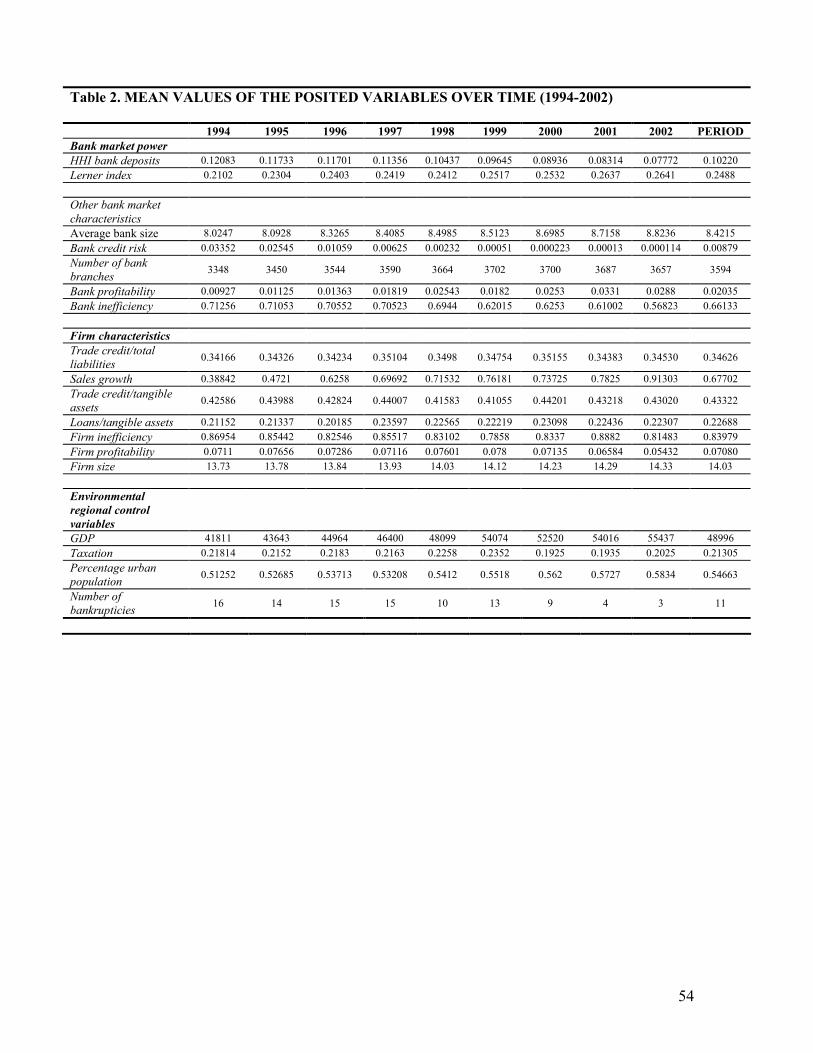
Table 2. MEAN VALUES OF THE POSITED VARIABLES OVER TIME (1994-2002)
1994 1995 1996 1997 1998 1999 2000 2001 2002 PERIOD
Table 10. SMEs Financing constraints and firm, bank market and environmental conditions.
PROBIT random effects panel data results. Dependent variable = 1 if the firm is financially constrained, 0 otherwise number of points in Hermite quadrature = 20 p-values in parenthesis (I) (II)
Esitmate
Economic
significance
(marginal effecta)
Esitmate
Economic
significance
(marginal effect a)
Constant 3.4174***
(0.000) -
3.3164***
(0.000) -
Bank market power
HHI bank deposits -0.39593**
(0.010) -35.42 - -
Lerner index - - 0.02889***
(0.000) 11.3
Other bank market characteristics
Average bank size -0.40918**
(0.042) -4.12
-0.62672**
(0.041) -4.26
Bank credit risk -2.5549***
(0.000) -4.62
-2.1420***
(0.000) -5.83
Number of bank branches -0.00016***
(0.000) -0.0085
-0.000159***
(0.001) -0.0091
Bank profitability -0.281142**
(0.032) -9.67
-0.13310
(0.315) -4.01
Bank inefficiency 0.08840***
(0.005) 0.56
0.01699***
(0.000) 0.98
Firm characteristics
Firm inefficiency 0.03413***
(0.004) 2.57
0.04880**
(0.011) 6.90
Firm profitability -0.09564***
(0.000) -3.13
-0.09535***
(0.000) -4.04
Firm size 0.27370***
(0.000) 7.85
0.26986***
(0.000) 7.82
Environmental regional control variables
GDP -0.13E-05***
(0.000) -0.067
-0.15E-05***
(0.000) -0.10
Taxation 0.00040
(0.550) 0.00097
0.00047
(0.488) 0.00010
Percentage urban population 0.20669***
(0.000) 0.95
0.22799***
(0.005) 0.91
Number of bankrupticies 0.01165**
(0.014) 0.58
0.00945***
(0.000) 0.51
ρ 0.82352***
(0.000)
0.82718***
(0.000)
LR (zero slopes) 6286.44
(0.000)
5238.25
(0.000)
Log likelihood -51920.8 -44813.9
Fraction of correct predictions (%) 69.19 68.78
Observations 278.073 278.073
Number of firms 30.897 30.897
(a) marginal effects in percentage points calculated at sample means * Statistically significant at 10% level ** Statistically significant at 5% level *** Statistically significant at 1% level
62
Table 11. Cash flow-investment correlations and financing constraints. Dependent variable: Capital expenditurest/