WP/07/215

Bank Ownership, Market Structure and Risk

Gianni De Nicolò and

Elena Loukoianova

1

© 2007 International Monetary Fund WP/07/215 IMF Working Paper Research Department

Bank Ownership, Market Structure and Risk

Prepared by Gianni De Nicolò and Elena Loukoianova1

Authorized for distribution by Krishna Srinivasan

September 2007

Abstract This Working Paper should not be reported as representing the views of the IMF. The views expressed in this Working Paper are those of the author(s) and do not necessarily represent those of the IMF or IMF policy. Working Papers describe research in progress by the author(s) and are published to elicit comments and to further debate.

This paper presents a model of a banking industry with heterogeneous banks that delivers predictions on the relationship between banks’ risk of failure, market structure, bank ownership, and banks’ screening and bankruptcy costs. These predictions are explored empirically using a panel of individual banks data and ownership information including more than 10,000 bank-year observations for 133 non-industrialized countries during the 1993-2004 period. Four main results obtain. First, the positive and significant relationship between bank concentration and bank risk of failure found in Boyd, De Nicolò and Al Jalal (2006) is stronger when bank ownership is taken into account, and it is strongest when state-owned banks have sizeable market shares. Second, conditional on country and firm specific characteristics, the risk profiles of foreign (state-owned) banks are significantly higher than (not significantly different from) those of private domestic banks. Third, private domestic banks do take on more risk as a result of larger market shares of both state-owned and foreign banks. Fourth, the model rationalizes this evidence if both state-owned and foreign banks have either larger screening and/or lower bankruptcy costs than private domestic banks, banks’ differences in market shares, screening or bankruptcy costs are not too large, and loan markets are sufficiently segmented across banks of different ownership. JEL Classification Numbers: G21, G32, L13 Keywords: Bank Ownership, Concentration, Risk Author’s E-Mail Address: gdenicolo@imf.org and eloukoianova@imf.org

1 We thank seminar participants at the IMF, the Said Business School at Oxford University, the European Central Bank, the Bank of Italy, the Federal Reserve Bank of New York, the Bank for International Settlements, the CFS-Deutsche Bundensbank-Wharton conference on “Public versus Private Ownership of Financial Institutions”, the 43rd.FED Chicago conference on Bank Structure and Competition, and especially Giorgio Gobbi, Alain Ize, Isabel Schnabel, Steve Seelig and Oren Sussman, for comments and suggestions.

2

Contents Page I. Introduction .......................................................................................................................... 3 II. The Model ........................................................................................................................... 5 A. Homogenous Banks ................................................................................................ 7 B. Heterogenous Banks................................................................................................ 9 III. A Helicopter Tour of the Data ......................................................................................... 13 A. Bank Asset Shares by Ownership ......................................................................... 14 B. Balance Sheet Composition .................................................................................. 14 C. Cost and Profitability ............................................................................................ 14 D. Capitalization and Loan Quality ........................................................................... 15 E. Summary................................................................................................................ 15 IV. Evidence .......................................................................................................................... 16 A. Regression Specifications ..................................................................................... 16 B. Z-score Regressions .............................................................................................. 19 C. Theory and Evidence............................................................................................. 20 D. Regressions of Z-score Components..................................................................... 21 E. Balance Sheet Composition Regressions .............................................................. 23 V. Conclusion ........................................................................................................................ 24 Appendix ................................................................................................................................ 26 References.............................................................................................................................. 30 Tables 1. Market Shares of Banks by Ownership ..................................................................... 32 2. Asset and Liability Composition ............................................................................... 34 3. Cost and Profitability ................................................................................................. 35 4. Loan Quality and Capitalization ................................................................................ 37 5. Description of Variables ............................................................................................ 38 6. Dependent Variable: Z(t) ........................................................................................... 39 7. Dependent Variable: ROA(t) ..................................................................................... 40 8. Dependent Variable: LEQTA(t) ................................................................................ 41 9. Dependent Variable: Ln [σ (ROA(t)]........................................................................ 42 10. Dependent Variable: LGTLA(t) ................................................................................ 43 11. Dependent Variable: LDEPL(t) ................................................................................. 44

3

I. INTRODUCTION

The entry of foreign banks in emerging and developing economies has been intense since the early 1990s. During the same period, privatizations of state-owned banks have been also undertaken in several countries, while consolidation has advanced in many banking industries around the world. Understanding the financial stability implications of bank state-ownership and the increasing presence of foreign banks in host countries is a high priority in policymakers’ agendas. Yet, the literature has focused primarily on comparisons of bank efficiency and on the implications of bank ownership for growth and the provision of credit. 2 To our knowledge, no study has explicitly examined the joint effects of bank ownership and market structure on banks’ risk profiles, and addressed the following questions: Do risk profiles of private domestic, state-owned and foreign banks differ significantly across market structures? Do private domestic banks take on more risk as a result of larger market shares of either foreign or state-owned banks? Answers to these questions are essential for understanding the implications of bank ownership and market structure for financial stability. This paper addresses these questions theoretically and empirically. It presents a model of a banking industry with heterogeneous banks that delivers predictions on the relationship between banks’ risk of failure, market structure, and bank screening and bankruptcy costs. The model guides the empirical analysis, in the sense that measures of market structure and bank risk are derived from the model, and a set of regressions is specified consistently with the model’s equilibrium conditions. The empirical analysis aims at gauging the impact of market structure and bank ownership on the risk profiles, profitability, volatility of earnings, and on uses and sources of funding of private domestic, state-owned and foreign banks. This analysis is carried out using a panel of individual banks data and ownership information including more than 10,000 bank-year observations for 133 non-industrialized countries during the 1993-2004 period. The results of this empirical analysis are interpreted in light of theory, identifying under which assumptions, if any, theory may rationalize the evidence.

The model has two main features. First, banks compete both in the loan and deposit markets, and both the firms that borrow from banks and the banks themselves are subject to moral hazard, as in Boyd and De Nicolò (2005). Second, banks differ in two dimensions: the efficiency of the screening technology to identify borrowers’ quality, and the level of bankruptcy costs. The latter costs are interpreted as embedding managerial reputation costs as well as implicit or explicit government guarantees. Bank differences in screening and bankruptcy costs are then mapped into different bank ownership. In equilibrium, the degree of bank heterogeneity may translate into either homogenous or heterogeneous responses of different banks to certain changes in parameters. If either banks’ 2 On entry and activities of foreign banks in emerging market economies, see Domanski (2005) and Committee on the Global Financial System (2004, 2005). On state-owned banks and privatizations, see Andrews (2005), La Porta and others (2002) and Boehmer, Nash and Netter (2005). On consolidation, see De Nicolò and others (2004).

4

screening and bankruptcy costs are markedly different among different bank types, then the model can predict bank responses of different sign. Conversely, if these bank characteristics are sufficiently similar, then the model can predict bank responses of the same sign. For example, a ceteris paribus increase in market shares of banks of a certain type may result in more risk taking of banks of a different type. This kind of negative “externality” underpins many conjectures often made in policy discussions about the effects of competition of banks of a certain type, say foreign banks, on the stability of banks of a different types, say private domestic banks. Another example is provided by De Nicolò (2000), who finds that private banks operating in industrialized countries with a larger share of bank assets under state-ownership exhibit higher insolvency risk. This finding suggests the possible existence of another type of “negative” externality affecting private domestic banks. The model identifies conditions under which such externalities may arise, and the empirical analysis aims at assessing whether these externalities are quantitatively relevant. The analysis of the data begins with simple tests of difference of unconditional means for measures of balance sheet composition, cost, profitability, capitalization, and loan quality of private domestic, state-owned and foreign banks. There are significant differences among private, state-owned, and foreign banks in terms of balance sheet composition and loan quality. In terms of profitability, costs, and capitalization, however, these differences vary greatly across countries, often with opposite signs. Subsequently, we present the results of a set of regressions that relate measures of overall and ownership-specific concentration measures to measures of bank risk of failure, profitability, volatility of earnings, capitalization, and asset and liabilities composition. These regressions also allow us to test differences of conditional means of all the indicators considered across bank ownership.

The following main results obtain. First, the positive and significant relationship between bank concentration and bank risk of failure found in Boyd, De Nicolò and Jalal (2006) (BDNJ henceforth) is stronger when bank ownership is taken into account, and it is strongest when state-owned banks have sizeable market shares. Second, conditional on country and firm specific characteristics, the risk profiles of foreign (state-owned) banks are on average significantly higher (not significantly different from) than those of private domestic banks. Third, private domestic banks do indeed take on more risk as a result of larger market shares of both state-owned and foreign banks. Lastly, the model rationalizes this evidence under the assumptions that both state-owned and foreign banks have either larger screening and/or monitoring costs or lower bankruptcy costs than private domestic banks, banks’ differences in market shares, screening or bankruptcy costs are not too large, and loan markets are sufficiently segmented across bank of different ownership. These assumptions are consistent with standard incentive theory under moral hazard, as well as with the evidence of many empirical analyses of individual country data available in the literature. The remainder of the paper is composed of four sections and an Appendix. Section II presents the model. Section III describes the data and carries out simple comparisons of unconditional means. Section IV presents the regression analysis, its results, and discusses under what conditions the model can rationalize the evidence. Section V concludes with a

5

brief discussion of broad policy implications. Proofs of all propositions are detailed in the Appendix.

II. THE MODEL

The economy is composed of three groups of agents: entrepreneurs, depositors and N banks. All agents are risk-neutral. There are two periods: 0 and 1.

Entrepreneurs There is a continuum of entrepreneurs indexed by ( , ) [0, ] [0,1]a b a x∈ . Parameter a indexes the productivity of an entrepreneur, while parameter b indexes her reservation utility level. Entrepreneurs have no initial resources but have access to a project that requires a fixed amount of date 0 investment, standardized to 1. The project yields a random return at date 1 as a function of effort exerted by the entrepreneur at date 0. Specifically, at date 1 the project yields ( )X a with probability (0,1)P∈ (the good state), and 0 otherwise, and projects returns are perfectly correlated across entrepreneurs, The output function in the good state ( )X a is assumed to satisfy ( ) 0X a > for all *[ , ]a a a∈ , with * 0a > , ( ) 0X a′ > and ( ) 0X a′′ < . An entrepreneur chooses P by incurring an effort cost of 20.5P , and such choice is unobservable to outsiders.

Entrepreneurs learn their productivity parameter a (their type) only after investing at date 0. Thus, the expected return of the project of any entrepreneur who has chosen a level of effort

P is 0

( ) ( )a

ER P X a g a da≡ ∫ , where ( )g a is the density of the distribution of entrepreneurs

over *[ , ]a a . We assume that ER is sufficiently small so that even with available financing at zero cost, no entrepreneur would undertake a project unless his productivity could be known prior to investing. The reservation utility level of any entrepreneur b is distributed on the unit interval with density (.)f and twice-differentiable, strictly increasing distribution function (.)F , with (.) 0F ′ > and (.) 0F ′′ ≤ .

Entrepreneurs of a certain productivity type a can be identified by banks at a screening cost prior to investing, and an entrepreneur’s productivity type becomes known to her once screened.3 If an entrepreneur can obtain a loan from a bank, this is granted under a simple debt contract. Such contract stipulates that if the project is successful, the bank receives a payment ( )R a . If the project is unsuccessful, the bank gets nothing. Under such contract, an entrepreneur would choose [0,1]P∈ to maximize:

2( ( ) ( )) 0.5P X a R a P− − (1) 3 The assumption that only banks can infer the entrepreneur’s productivity type by screening is made for simplicity, and can be viewed as the mirror image of the assumption that only entrepreneurs can screen their projects made in Bernanke and Gertler (1990).

6

The unique interior solution to (1) satisfies:

( , ) ( ) ( )P R a X a R a= − (2),

and the relevant profit is given by 20.5( ( ) ( ))X a R a− . An entrepreneur ( , )a b who does not undertake the project attains a utility level b . Thus, an entrepreneur with reservation utility level b will accept the loan and undertake the project if

20.5( ( ) ( ))X a R a b− ≥ (3)

Let *b denote the value of b that satisfies (3) at equality, and let 1(.) (.)g F −≡ . If type- a

entrepreneurs are financed, the total demand for loans is given by *

*

0

( ) ( )b

L F b f b db≡ = ∫ .

This expression defines implicitly the inverse loan demand function of type- a entrepreneurs:

12( , ) ( ) 2 ( )R L a X a g L= − (4)

The partial derivatives of this function satisfy 0LR < , ( ) 0aR X a′= > , while the cross partial derivatives are zero. Substituting (4) in (2), the probability of a successful outcome is

12( ) 2 ( )P L g L= (5),

which satisfies 0P′ > and 0P′′ < . Depositors Depositors cannot observe entrepreneurs’ types. Thus, they do not finance entrepreneurs directly. Instead, they deposit their funds in a bank at date 0 to receive interest plus principal at date 1. Deposits are fully insured, so that the total supply of deposits does not depend on risk, and it is represented by an upward sloping inverse supply curve, denoted by ( )Dr ⋅ , which is assumed to satisfy 0Dr′ > and 0Dr′′ ≥ .

Banks On the funding side, banks collect insured deposits, and for this insurance, they pay a flat rate insurance premium, standardized to zero. On the lending side, banks choose which type of entrepreneurs to finance, and provide funds to them through simple debt contracts. Specifically, banks can identify entrepreneurs of type a at a “screening” cost aσ per unit invested. Thus, higher screening costs are incurred to identify entrepreneurs of higher quality. As noted, once screened by a bank, entrepreneurs learn their productivity type. However, banks cannot observe entrepreneurs’ effort choice P . In setting the lending rate,

7

they take into account the best choice of effort of entrepreneurs in response to any offered loan rate.

Since banks invest only in loans, if the borrowers of a bank default, the bank itself defaults. In such an event, a bank incurs a “bankruptcy” costs per unit lent 0γ > . As noted, this cost can be interpreted as capturing net managerial reputation costs as well as implicit or explicit government guarantees.

The mechanics of the model with heterogeneous banks is best illustrated by analyzing first the version of the model with homogenous banks, which is described next.

A. Homogenous Banks

Suppose all banks incur the same screening, monitoring and bankruptcy costs per unit lent. Let iD denote total deposits of bank i ,

1

Nii

Z D=

≡ ∑ denote total deposits and i jj iD D− ≠

≡ ∑

denote the sum of deposits chosen by all banks except bank i . Each bank chooses the entrepreneur type to finance (parameter a ) and the amount of deposits to lend so as to maximize profits, given similar choices of the other banks and taking into account the entrepreneurs’ choice of P .

Thus, each bank chooses ( ) 2,a D R+∈ to maximize

( )( ) ( )( , ) ( ) (1 )i i D i iP D D R D D a r D D D P D D D aDγ σ− − − −+ + − + − − + − (6)

Let Z ND≡ denote total deposits, which equal total loans in equilibrium. Under the assumption that the objective function (6) is strictly concave in D , an interior symmetric Nash equilibrium is characterized by the following conditions:

( ) ( ) ( ), , , , , 0DR Z a r Z F Z a Nγ σ γ− + − = (7),

( ) ( ) 0P Z X a σ′ − = (8), where

( ) ( ) ( )( )( )

, ( ) ( ), , , ,

( )D Zr Z R Z a P Z Z a N

F Z a NP Z Z P Z N

γ σσ γ

′ − + +≡

′ +. (9)

By the monotonicity of function (.)X ′ , equation (8) can be inverted to yield the equilibrium choice of a as a function of total deposits and the screening cost parameter:. .

1( / ( )) ( / ( ))a X P Z g P Zσ σ−′= ≡ (10).

8

Note that / ( ) 0a g P Zσ ′= < since 0g′ < : for any given total amount of deposits, a is decreasing in screening costs σ . Note also that changes in a are positively associated with changes in total deposits Z , since 2( ) /( ( )) 0Za g P Z P Z′ ′= − > ,

Substituting (10) in (7), we get

( ) ( ) ( )ˆ ˆ, , , , 0DR Z r Z a F Z Nσ μ γ σ γ− − + − = (11),

where ( )ˆ , ( , ( / ( ))R Z R Z g P Zσ σ≡ and ( ) ( )ˆ , , , , ( / ( )), , ,F Z N F Z g P Z Nσ γ σ σ γ≡ .

Totally differentiating equations (11) with respect to Z and the parameters N , σ , and γ , we obtain:

ˆ ˆ ˆ ˆ ˆ ˆ( ) ( ) ( 1)Z D Z NR r F dZ F dN F R d ad F dσ σ γσ μ γ′− − = + − + + − (12),

Recall that the equilibrium probability of a successful outcome 12( ) 2 ( )P Z g Z= (equation

(5)) and the equilibrium choice of a (equation (10)) are uniquely determined by, and strictly increases in, the equilibrium level of total deposits, Z . Therefore, the sign of dP and that of da ) are the same as the sign of dZ . , The comparative statics results with respect to N and σ are summarized in the following:

Proposition 1

(a) If 0dN > and 0d dσ γ= = , then 0dZ > , 0dP > and 0da > ;

(b) If 0dσ < and 0dN dγ= = , then 0dZ > , 0dP > and 0da > .

The interpretation of these results is straightforward. As N increases (part(a)) competition increases. Hence, total deposits increase and bank risk of failure decreases (1 P− decreases). This result is, essentially, that obtained by Boyd and De Nicolò (2005). When competition increases, banks charge lower loan rates, thereby giving entrepreneurs an incentive to take on less risk. Similarly, as screening costs σ decline (part (b)), banks’ optimally choose entrepreneurs of better quality (a larger a ), and such quality’s improvement entails an upward shift of the inverse supply schedule (see equation (4)). As a result, banks expand total deposits, and their risk of failure (1 P− ) declines.

Differing from the foregoing results, the comparative statics with respect to bankruptcy costs γ can be non-monotonic, as shown in the following

Proposition 2 Let MZ denote the total amount of deposits chosen by a monopolist and let 0dγ > and 0dN dσ= = . If 1 ( ) ( )M M MP Z Z P Z′< + , then 0dZ > , 0dP > and 0da > for

all N N< ,, while 0dZ < , 0dP < and 0da < for all N N> .

9

This result establishes an important interdependence between the degree of competition and the risk incentives associated with variations in bankruptcy costs. Recall that an increase (decrease) in these costs may be viewed as associated with smaller (larger) safety net guarantees and/or higher (lower) managerial reputation costs.

When the degree of competition is relatively low ( N is not too large), as bankruptcy costs γ increase, the marginal option value of limited liability net of bankruptcy costs decreases. This gives banks an incentive to increase their expected profits by reducing their risk of failure through charging lower loan rates. In essence, this is the well known risk shifting result typically obtained by considering an individual firm and assuming there are no strategic interactions among firms. However, this result is reversed when the degree of competition is relatively high ( N is sufficiently large). In this case, the marginal option value of limited liability net of bankruptcy costs increases, giving banks an incentive to rise expected profits by taking more risk through charging higher loan rates.

B. Heterogeneous Banks

We now consider two types of banks, indexed by 1,2j = , which differ with respect to the “efficiency” of their screening technology ( 1 2σ σ≠ ) and the “size” of their bankruptcy costs ( 1 2γ γ≠ ).

Let ji kk i

D D− ≠≡∑ denote the sum of deposits chosen by all type-j banks except type-j bank

i . As before, each bank chooses the entrepreneur type and deposits so as to maximize profits, given similar choices of the other banks and taking into account the entrepreneurs’ choice of P . Note that in choosing the type of entrepreneurs to finance, each bank type effectively chooses a different loan demand function. Loan markets are therefore endogenously segmented, and no entrepreneur of any type different from the one chosen by a bank type will ever be financed by any other bank type. Thus, the strategic interaction of banks of different types in the loan market is indirect, since it passes through the channel of competition in the deposit market. Of course, banks of the same type compete directly in both loan and deposit markets.

Thus, each type-j bank chooses ( ) 2,a D R+∈ to maximize

( )( ) ( )( , ) ( ) (1 )j j j j ji i D i i j jP D D R D D a r D D D P D D D aDγ σ− − − −+ + − + − − + − (13.j).

Denote with j j jZ N D≡ total bank-j deposits (equal to total bank-j loans in equilibrium), and with 1 2Z Z Z≡ + total deposits. For j=1,2, an interior symmetric Nash equilibrium is characterized by the following conditions:

( ) ( )1 2 1 2, ( , , , , , ) 0jj j D j j j j jR Z a r Z Z F Z Z a Nγ σ γ− + + − = (14.j),

( ) ( ) 0j j jP Z X a σ′ − = (15.j),

10

where

( ) ( )( )

( )1 2

1 2

, ( ) ( )( , , , , , )

( )jD Z j j j j j j j jj

j j j jj j j j

r Z Z R Z a P Z Z a NF Z Z a N

P Z Z P Z N

γ σσ γ

′ + − + +≡

′ +. (16.j)

Following the procedure described previously, we substitute the optimal level of a implied by (15.j) in (14.j) and (16.j), for j=1,2, and define:

( )ˆ , ( , ( / ( ))j j j j j jR Z R Z g P Zσ σ≡ , and

( ) ( )1 2 1 2ˆ , , , , , , ( / ( )), , ,j

j j j j j j j j jF Z Z N F Z Z g P Z Nσ γ σ σ γ≡ .

Totally differentiating the resulting equations (13.j) and (14.j) with respect to jZ the parameters jN , jσ , and jγ , for j=1,2, we get

1 1 2 1 1 1 1

1 1 1 1 11 2 1 1 1

ˆ ˆ ˆ ˆ ˆ ˆ ˆ( ) ( ) ( ) ( 1)Z D Z D Z NR r F dZ r F dZ F dN F R d F d Hσ σ γσ γ′ ′− − − + = + − + − ≡ ( 17),

1 2 2 2 2 2 2

2 2 2 2 21 2 2 2 2

ˆ ˆ ˆ ˆ ˆ ˆ ˆ( ) ( ) ( ) ( 1)D Z Z D Z Nr F dZ R r F dZ F dN F R d F d Hσ σ γσ γ′ ′− + + − − = + − + − ≡ (18)

Let Δ denote the determinant of system (16)-(17). Applying Cramer rule, we get

2 2 2

1 1 1 2 11

ˆ ˆ ˆ[ ( ) ( )]Z D Z D ZdZ H R r F H r F− ′ ′= Δ − − + + (19),

and 1 1 1

1 2 1 1 22

ˆ ˆ ˆ[ ( ) ( )]Z D Z D ZdZ H R r F H r F− ′ ′= Δ − − + + . (20).

The sign of the determinant Δ depends on the size of the curvature of banks’ revenue functions. For example, if ˆ ˆ ˆ| |

j j k

j jZ D Z D ZR r F r F′ ′− − > + for j,k=1,2, j k≠ , then Δ is strictly

positive. In what follows we assume 0Δ > , noting that if 0Δ < all results reported below hold with all implications reversed.

The comparative statics results with respect to changes in the number of banks are summarized in the following:

Proposition 3 Assume 0Δ > , and let 1 0dN > , 2 0dN > and 0j jd dσ γ= = , j=1,2.

(a) If 1 2 1/ (0, )dN dN A∈ , then 1 0dZ < , 1 0dP < , 1 0da < , and 2 0dZ > , 2 0dP > , 2 0da > ;

11

(b) If 1 2 1 2/ ( , )dN dN A A∈ , then 1 0dZ > , 1 0dP > , 1 0da > , and 2 0dZ > , 2 0dP > , 2 0da > ;

(c) If 1 2 2/dN dN A> , then 1 0dZ > , 1 0dP > , 1 0da > , and 2 0dZ < , 2 0dP < , 2 0da < ,

where 2 1 2 1 1

1 2 2 1 2

2 2 2 1

1 21 2 1 1

ˆ ˆ ˆ ˆ ˆ( ) ( )0 ˆ ˆ ˆ ˆ ˆ( ) ( )

N D Z N Z D Z

N Z D Z N D Z

F r F F R r FA A

F R r F F r F

′ ′+ − −< ≡ − < ≡ −

′ ′− − +. 4

Unlike the homogenous case, an increase in competition due to an increase in the number of both types of banks may result in either similar or different banks’ risk taking responses. Specifically, these responses will be similar (different) the smaller (larger) is the relative change in the number of banks. This is because when the number of banks of both types increases, the increase in competition in the deposit market will be symmetric for both bank types since they experience the same increase in funding costs, but it will be asymmetric in the loan market, since they choose different loan demand schedules, hence different marginal revenues. The asymmetric effect will dominate on net, generating different risk responses, the largest is the asymmetry in the change in the number of banks (parts (a)and (c)), while the symmetry effect will dominate on net whenever the relative change in the number of banks is not too large or too small (part (b)).

This result can be further explained as follows. As the increase in the number of type-1 banks is small relative to that of type-2 banks (part (a)), total deposits of both bank types increase, raising their funding costs symmetrically. However, type-1 banks’ reduction in revenues due to increased competition in the loan market is proportionally smaller than the corresponding reduction in revenues for type-2 banks. Thus, type-1 banks will have an incentive to reduce lending, increase lending rates and risk, since at the margin, the improvement in expected profits obtainable from this strategy is superior to the alternative of increasing lending and decreasing risk. The same mechanism, but in reverse, holds for type-2 banks, who will increase lending and decrease risk. Of course, the same effects, with the type of banks interchanged, will hold when the increase in the number of type-2 banks is small relative to that of type-1 banks (part (c)). In both these cases, the asymmetric change in competition in loan markets dominates. By contrast, if the relative changes in the number of banks is not too large (part (b)), the change in risk for both type of banks will move in the same direction. In this case, a uniform, albeit “asymmetric” increase in competition will generate a result similar qualitatively to the one obtained in the homogenous case, although the size of changes in deposit demand, supply and risk of failure of different bank types will clearly differ.

Similar results hold when screening costs change, but the range of variations differ from those defined previously, as shown in the following proposition:,

Proposition 4 Assume 0Δ > and let 1 0dσ < , 2 0dσ < and 0j jdN dγ= = , j=1,2. 4 Note that the comparative statics formulation of this proposition and those that follow include the case of changing one parameter of a bank type keeping the parameters of the other bank type fixed

12

(a) If 1 2 1/ (0, )d d Bσ σ ∈ , then 1 0dZ < , 1 0dP < , 1 0da < , and 2 0dZ > , 2 0dP > , 2 0da > ;

(b). If 1 2 1 2/ ( , )d d B Bσ σ ∈ , then 1 0dZ > , 1 0dP > , 1 0da > , and 2 0dZ > , 2 0dP > , 2 0da > ;

(c). If 1 2 2/d d Bσ σ > , then 1 0dZ > , 1 0dP > , 1 0da > , and 2 0dZ < , 2 0dP < , 2 0da < ,

where 2 2 1 2 2 1 1

1 1 2 2 1 1 1

2 12 2

1 22 2

ˆ ˆ ˆ ˆ ˆ ˆ ˆ( ) ( ) ( ) ( )0 ˆ ˆ ˆ ˆ ˆ ˆ ˆ( )( ) ( )( )

D Z Z D Z

Z D Z D Z

F R a r F F R a R r FB B

F R R r F F R r Fσ σ σ σ

σ σ σ σ

′ ′− + − − −< ≡ − < ≡ −

′ ′− − − − +

It is important to note that an improvement in entrepreneurs’ quality due to a decline in screening costs of both bank types does not necessarily imply a reduction in bank risk (as in the model with homogenous banks), since banks trade-off at the margin both the marginal benefits of improving entrepreneurs’ quality and the rents that are obtainable from changes in market power in both loans and deposit markets .

Lastly, results qualitatively similar to the previous ones obtain when we consider changes in bankruptcy costs for both bank types. Here, however, we need to take into account the fact that the sign of banks’ responses will change depending on whether or not the number of banks of each type is below or above the relevant threshold levels jN as defined in Proposition 2.

Proposition 5 Assume 0Δ > ; 1 ( ) ( )jM jM jMP Z Z P Z′< + , j=1,2, and let 1 0dγ > , 2 0dγ > and 0j jdN dσ= = , j=1.2. Furthermore, let

2 1

1 2 2

2 2

1 1 2

ˆ ˆ( 1)( )ˆ ˆ ˆ( 1)( )

D Z

Z D Z

F r FC

F R r Fγ

γ

′− +≡ −

′− − − ; 2 1 1

1 1

2 1

2 1 2

ˆ ˆ ˆ( 1)( )ˆ ˆ( 1)( )

Z D Z

D Z

F R r FC

F r Fγ

γ

′− − −≡ −

′− +;

(i) 1 0C > and 2 0C > ; and (ii) 1 0C < and 2 0C < ,

(a) If (i) and 1 2 1/ (0, )d d Cγ γ ∈ , then 1 0dZ > , 1 0dP > , 1 0da > , and

2 0dZ < , 2 0dP < , 2 0da < ;

(b). If (i) and 1 2 1 2/ ( , )d d C Cγ γ ∈ , then 1 0dZ > , 1 0dP > , 1 0da > , and

2 0dZ > , 2 0dP > , 2 0da > ;

(c). If (i) and 1 2 2/d d Cγ γ > , then 1 0dZ > , 1 0dP > , 1 0da > , and 2 0dZ < , 2 0dP < , 2 0da <

(d) If (ii) and 1 2/ 0d dγ γ > , then 1 0dZ > , 1 0dP > , 1 0da > , and 2 0dZ < , 2 0dP < , 2 0da < .

13

As in the case of changes in screening costs, note that an increase in bankruptcy costs does not necessarily imply a reduction in bank risk, since banks trade-off at the margin both the benefits of the option value of limited liability net of bankruptcy costs and the rents that derive from changes in market power in both loans and deposit markets.

In sum, this model predicts either similar or different changes in the risk profiles of different types of banks in response to changes in parameters. In reality, variations in the degree of competition and in screening and bankruptcy costs may occur simultaneously, and the model can yield a wide variety of predictions depending on the relative size of changes of parameters. However, the key difference among these predictions is whether changes in risk profiles of different types of banks will move in opposite or similar directions.

The empirical analysis, to which we now turn, reveals which of these two possibilities is consistent with the data, and which changes in parameter configurations of the model, if any, can rationalize the evidence when differences in banks’ screening and bankruptcy costs are mapped into different ownership structures.

III. A HELICOPTER TOUR OF THE DATA

We consider individual banks data for 133 countries excluding major developed countries for the 1993-2004 period taken from the Fitch IBCA’s Bank Scope database. There are between 10,000 and 18,000 bank-year observations with unconsolidated balance sheet information in our sample, depending on the availability of specific variables. The majority ownership of banks is identified using information from Bankscope, annual reports and other public information sources. We also cross-checked and used the ownership information contained in the smaller dataset for non-developed economies constructed by Micco, Panizza, and Yanez (2006), as well as the privatization database used by Boehmer, Nash and Netter (2005),5 and integrated this information with our dataset.

As our dataset on ownership information for non-industrialized economies is substantially larger than any other used in the literature to date, we find it informative to compare several indicators of bank asset shares by ownership, and examine differences in unconditional means of balance sheet composition indicators, costs and profitability, loan quality and capitalization.6 Statistics for these indicators are reported for the full sample, as well as for countries grouped by PPP-adjusted GDP per capita levels and by the following geographical regions: Africa, Middle East, Commonwealth of Independent States (CIS), Central and Eastern Europe and Baltics (CEEB), Central America and Caribbean, South America, and Far East and Asia.

5 We thank Ugo Panizza and Robert Nash for sharing their bank ownership and privatization data sets.

6 In terms of bank-year observations, our sample is about 15 percent smaller than the sample used in BDNJ, owing to our inability to classify the ownership of all banks.

14

A. Bank Asset Shares by Ownership

Table 1 reports the evolution of bank asset shares by ownership since 1994. For the entire sample, the share of foreign-owned banks in the total sample increased, whereas the share of private and state-owned banks declined. While the share of foreign banks increased across all income groups except low-middle income group ( i.e. countries with income between US$3,175 to US$5,860 at PPP), that of state-owned banks declined over time in the low income group, while it increased in other income groups. When these changes are examined by region, the share of foreign banks increased on average in most regions, while the share of state-owned banks has on average increased or not changed with the exception of Africa.

In sum, despite the notable increase in the number of privatization in some countries, the market share of state-owned banks remains still significant.

B. Balance Sheet Composition

On the asset side, the (gross) loan-to-asset ratio of state-owned banks is uniformly lower than that of both private domestic banks and foreign banks in total, as well as by income level and region (Table 2.1), with the exception of the high-middle income group and Middle East. This may in part reflect the role of state-owned banks in absorbing government issued bonds in most countries. On the other hand, the loan-to-asset ratio of private domestic banks is on average higher than that of foreign banks except in the CEEB region.7 Yet, we note that differences in loan allocations among the two groups are not large quantitatively in most regions, except in the CIS.

On the liability side (Table 2.2), state-owned banks exhibit a ratio of deposits to liabilities lower that of private domestic and foreign banks in the total sample and in all subgroups. Thus, deposits as a source of funding appear relatively less important for state-owned banks. By contrast, this ratio is uniformly higher for private domestic banks relative to foreign banks in the total sample and all subgroups, as well as in all regions except Africa, the CIS, and the CEEB.

C. Cost and Profitability

The cost-to-income ratios of state-owned banks are lower than those of private domestic and foreign banks in the total sample and for all income groups except the highest income group, where state-owned banks exhibit ratios higher than those of private domestic banks (Table 3.1). Yet, a great deal of heterogeneity emerges when we compare these ratios across regions. State-owned banks have ratios significantly higher than both private domestic and foreign banks in Central and South America, while they are significantly lower in the Middle East and the CEEB. Similarly, the same degree of heterogeneity is apparent when comparing these ratios for private domestic and foreign banks, whose differences vary both by income group and region. 7 Using a substantially smaller sample for the period 1996-2000 and a slightly different country and bank classification, Bonin and others (2005) find essentially the same patterns.

15

Regarding indicators of profitability, net interest margins of foreign and private domestic banks are higher than those of state-owned banks in all income groups, and all regions (Table 3.2) with the exception of CEEB, where state-owned banks exhibit a higher net interest margin than foreign banks. Foreign banks have a lower net interest margin than private domestic banks in the high middle income group, CIS, CEEB, and South America regions, while the reverse is true in the total sample as well as the rest of the subgroups.8

Return on average assets in the total sample is lower for state-owned banks than for foreign and private domestic banks (Tables 3.3), while return on average equity is lower for foreign banks than for state-owned and private domestic banks (Table 3.4). However, private domestic banks have a lower return on average assets than foreign banks in high middle income group, Middle East, and CIS. State-owned banks have higher return on average equity than private domestic banks in the CIS, the CEEB, and Far East and Asia, and in low income group. Also, private banks have a lower return on average equity than foreign banks in the low, middle, and high middle income groups, Middle East, CEEB, Central America and Caribbean, and Far East and Asia. The reverse relations holds for Africa, CIS, and South America.

Overall, heterogeneity in relative profitability of banks of different ownership across income levels and regions is pervasive.

D. Capitalization and Loan Quality

The capitalization of state-owned banks is significantly lower than that of private and foreign banks in the total sample, as well as in all income groups and most regions with the notable exception of Africa (Table 4.2), where these relationships are reversed. On the other hand, foreign banks exhibit a capitalization higher than private banks in the total sample, in most income groups and in the Africa, Middle East, Far East and Asia, and South America regions. Regarding loan quality, we should observe that reported non-performing loans are notoriously difficult to compare across countries and we have information on only about one half of bank-year observations in our sample. Keeping these caveats in mind, we note that state-owned banks exhibit ratios of non-performing loans to total loans higher than those of private and foreign banks in the total sample, as well as in all income subgroups (Table 4.1), but these differences are not significant in several regions. On the other hand, private domestic banks exhibit a ratio higher than that of foreign banks in the high middle income group, as well as in the Africa, Middle East, CIS, and CEEB regions.

E. Summary

The picture emerging from these comparisons is one of significant differences among private, state-owned and foreign banks in terms of balance sheet compositions and loan 8 The studies by Micco and others (2006), Bonin and others (2005), and Claessens and others (2001) find broadly the same empirical regularities using smaller samples and/or different time periods.

16

quality, but also heterogeneity of these differences across both income groups and regions in terms of profitability, costs and capitalization. Yet, the differences identified here only pertain comparisons of unconditional means. Next, we turn to regressions which present comparisons and determinants of bank risk measures, their components, and asset and liability structure conditional on market structure, country and firm characteristics.

IV. EVIDENCE

Our measure of bank risk is proxy of banks’ probability of failure. As in BDNJ, bank risk is measured by a Z-score defined at each date as ( ) / ( )t t t tZ ROA EQTA ROAσ= + , where tROA is the return on average assets, tEQTA is the equity-to-assets ratio, and

1( ) | |t t ttROA ROA T ROAσ −= − ∑ .

Market structure and the relevant degree of competition are measured with concentration measures inclusive of all banks analyzed and conditional on bank ownership, given by the Hirschmann-Hirfendahl Indices (HHIs). A limitation of the HHI as a measure of competitive conditions is that the relevant market for each bank in a country is identified with the country itself. This is why we did not include in the sample banks from the U.S., Western Europe and Japan, since in these cases defining the nation as a market is problematic both because of the country’s economic size and because of the presence of many international banks.

Empirical counterparts of versions of the equilibrium conditions of our model are given by the specifications of panel regression models described next.

A. Regression Specifications

Let the dependent variable ijtX denote the Z-score, or one of its components, of bank’s i in country j at date t . The square asset market share of bank i in country j at date t is denoted by 2

ijtS , and the HHI index of country j at date t is given by 2jt ijti

HHI S≡∑ . Let private domestic, state-owned , foreign banks and unclassified banks be indexed by

{ , , , }k B P S F U∈ ≡ , and denote with kI the relevant indicator functions.

The first set of regressions is given by the following country fixed effects specifications:

(1) 1 1 1ijt j j jt jt ijt ijtjX a I A HHI Y Zβ γ δ ε− − −= + + + + +∑

(2) 1 1 1{ }ijt j j k k jt jt ijt ijtj k B UX a I A I HHI Y Zβ γ δ ε− − −∈ −

= + + + + +∑ ∑

(3) 1 1 1{ } { }ijt j j k k k k jt jt ijt ijtj k B U k B UX a I A I I HHI Y Zβ γ δ ε− − −∈ − ∈ −

= + + + + +∑ ∑ ∑

The coefficients ja are country-specific intercepts, where jI denotes the relevant indicator functions. The kA coefficients are conditional means of the dependent variable by ownership. The coefficients β s measure the impact of a change in HHI on the dependent variable next

17

period. jtY is a vector of country-specific controls and ijtZ a vector of bank-specific controls as of date t , which we detail below. All right-hand side time-varying variables are lagged one year so as to capture variations in the dependent variable as a function of pre-determined past values of independent variables.

In regression (1) the conditional means and the coefficient β are restricted to be the same, that is, irrespective of bank ownership. In regression (2) we allow the conditional means to differ by ownership, while in regression (3) both the conditional means and the coefficient

sβ are allowed to vary by ownership. These three regressions allows us to gauge the extent to which the relationship between the dependent variable and HHI varies when bank ownership is taken into account, and to test differences in the conditional means of the dependent variable.

The second set of regressions is the same as the first, except that we control for time invariant firm specific effects:

(4) 1 1 1ijt i jt jt ijt ijtX a HHI Y Zβ γ δ ε− − −= + + + +

(5) 1 1 1{ }ijt i k k jt jt ijt ijtk B UX a I HHI Y Zβ γ δ ε− − −∈ −

= + + + +∑

In regression (4) , as in (2), we restrict the coefficient β to be ownership invariant, while in regression (5), as in (3), we allow the conditional means to differ by ownership. The results of these regressions are compared to regressions (2) and (3) to assess whether the relationship between the dependent variable and HHI continues to hold when a full set of time-invariant controls is introduced.

As noted, the regressions described so far can be interpreted broadly as statistical models consistent with the conditions characterizing Nash equilibria in our model. Yet, as illustrated in the model with heterogeneous banks, the effects of changes in parameters on the equilibrium choices of banks of each type can be either similar or different. Thus, we wish to measure the effects of changes in HHI on risk profiles when these changes are the result of changes in the combined market shares of all competitors of a banks of a given ownership type. To this end, we construct the concentration index 2

ijt mjtm iHHIC S

≠≡∑ , which measures

concentration of all competitors of bank i , and indexes 2,

kijt mjtm i m k

HHIC S≠ ∈

≡∑ , which

measure concentration of all type- k competitors of bank i . Of course, such indexes satisfy kijt ijtk B

HHIC HHIC∈

=∑ .

Furthermore, let “ controls ” denote 21 1 1 1

Ui k k ijt U ijt jt ijtk B

a I S HHIC Y Zα β γ δ− − − −∈+ + + +∑ , where

we control for a bank’s market share by ownership and for the HHI of unclassified banks, in addition to country-specific and firm specific variables,. The third set of regressions is given by

(6) ( ) 1{ }P

ijt kP SF k ijt ijtk B UX I HHIC controlsβ ε−∈ −

= + +∑

18

(7) ( ) 1{ }S

ijt kS PF k ijt ijtk B UX I HHIC controlsβ ε−∈ −

= + +∑

(8) ( ) 1{ }F

ijt kF PS k ijt ijtk B UX I HHIC controlsβ ε−∈ −

= + +∑

Coefficients ( )kl qvβ measure the sensitivity of the dependent variable of a type k bank to a change in the HHI of type- l competitors, when such a change is counterbalanced by a decrease in the sum of the HHIs of type- q and type- v competitors.9 For example, coefficient ( )PS PFβ measures the sensitivity of the dependent variable of a private domestic to a change in the HHI of state-owned bank competitors when this change is counterbalanced by a decline in the sum of the HHIs of private domestic and foreign bank competitors. These regressions allow us to gauge the extent of strategic interactions among banks of different ownership when the change in the HHI of one type competitor are occurring at the expense of the market shares of either one, or both other types’ competitors.

In addition, the informational content of the above regressions can be enhanced by considering counterbalancing changes of HHIs of one type of bank only. The last set of regressions is thus given by:

(9) ( ) 1 ( ) 1{ }P S

ijt kP F k ijt kS F k ijt ijtk B U k BX I HHIC I HHIC controlsβ β ε− −∈ − ∈

= + + +∑ ∑

(10) ( ) 1 ( ) 1{ }P F

ijt kP S k ijt kF S k ijt ijtk B U k BX I HHIC I HHIC controlsβ β ε− −∈ − ∈

= + + +∑ ∑

(11) ( ) 1 ( ) 1{ } { }S F

ijt kS P k ijt kF S k ijt ijtk B U k B UX I HHIC I HHIC controlsβ β ε− −∈ − ∈ −

= + + +∑ ∑

Here, coefficients ( )kl qβ measure the sensitivity of the dependent variable of a type k bank to a change in the HHI of type- l competitors, when such a change is counterbalanced by a decrease in the HHIs of type- q competitors. For example, coefficient ( )PS Fβ measures the sensitivity of the dependent variable of a private domestic to a change in the HHI of state-owned bank competitors conditional on the HHI of private domestic banks competitors being constant, when this change is counterbalanced by a decline in the HHIs of foreign bank competitors. These regressions complement regressions (6)-(8) since they allow us to gauge the strategic interactions among banks of different ownership when the increase (decrease) in the HHI of one type competitor are counterbalanced by a decline (increase) in the HHI of only one other bank type competitor.

In all regressions, the country-specific variables that control for cross-country differences in the evolution of the macroeconomy, in the supply of and demand for banking services and for market size are GDP per capita at PPP, real GDP growth, inflation and the nominal

9 Recall that the market shares of N firms or groups are linearly dependent. Therefore, convex functions of these shares, such as the HHIs, are (non-linearly) dependent.

19

exchange rate. Cross-country differences in the risks of the macroeconomic environment are controlled for with the volatility of GDP growth, inflation and the nominal exchange rate. The firm-specific variables are the logarithm of asset size, and the loan-to-asset, deposits- to-liabilities and cost-to-income ratios, which control for banks’ differences in size, asset and liability structure, and cost efficiency. The definitions of all variables are summarized in Table 5. As our focus is on estimates of parameters A s and β s, to save on space we do not report estimates of the coefficients of the control variables.

B. Z-Score Regressions

The regressions with the Z-score as the dependent variable are presented in Table 6. As in BDNJ, the relationship between bank risk and concentration is positive (recall that a decrease in the Z-score denotes higher risk) and significant in both regressions (1) and (4). Importantly, this positive and significant relationship also holds when we use a measure of loan portfolio risk, given by the ratio of non-performing loans to gross loans,10 as well as when we use an indicator of systemic risk in the banking system, given by the average Z-score across banks (Table 6, Appendix).

When we control for bank ownership, the coefficient β (regression (2)) and those associated with each bank type becomes larger in absolute value in both regressions (2) and (3), indicating that such positive relationship is stronger when bank ownership is taken into account. Furthermore, note that the coefficients associated with HHI satisfy 0 F P Sβ β β≥ > > (regressions (3) and (5)). Thus, the coefficient of state-owned banks is the largest in absolute value, the second largest is that of private domestic banks, while that of foreign banks is not significantly different from zero at standard significance levels. Overall, these results indicate that the positive impact of concentration on bank risk profiles is the largest, the larger is the market share of state-owned banks.

With regard to conditional means, the Z-score’s mean of state-owned banks is significantly lower than that of private domestic banks in regression (2), but becomes not significantly different from that of private domestic banks’ in regression (3). This result indicates that comparisons of conditional means that do not take into account differences in both market and ownership structures may conceal important information. Effectively, the comparatively higher conditional mean of the risk profiles of state-owned banks found with regression (2) appears primarily driven by market structure, that is, it depends on whether state-owned banks have or do not have significant market shares. By contrast, the conditional mean of the Z-score of foreign banks is significantly lower than that of private banks in both regressions (2) and (3), indicating significantly higher risk profiles for these banks compared to private domestic banks.

Next, we consider the coefficients measuring the (strategic) risk interactions among private domestic, state-owned and foreign banks (regressions 6-11).

10 Note that in this case the size of the sample is reduced by about a half owing to data availability.

20

Private domestic banks increase risk most, and significantly so, in response to an increase in the HHI of foreign bank competitors (coefficients (.)PFβ ); their second largest, and significant, increase in risk is in response to an increase in the HHI of state-owned bank competitors (coefficients (.)PSβ ) . By contrast, the coefficients measuring their change in risk in response to changes in the HHI of private domestic bank competitors are not significantly different from zero ( coefficients (.)PPβ ).

Turning to state-owned banks, they increase risk most when the HHI of state-owned bank competitors increase (coefficients (.)SSβ ). Moreover, they increase risk in response to an increase in the HHI of private domestic bank competitors, but they decrease it in response to an increase in the HHI of foreign bank competitors.11 Yet, both sets of coefficients associated with these responses (coefficients (.)SPβ and (.)SFβ ) are not statistically significant at conventional confidence levels.

Finally, foreign banks decrease risk in response to a positive change in the HHI of private domestic bank competitors, but increase risk in response to a positive change in the HHI of state-owned bank competitors, although the relevant set of coefficients (.)FPβ and (.)FSβ ) are not statistically significant. Interestingly, they also decrease risk in response to an increase in the HHI of their foreign bank competitors.

For robustness, we run all the above regressions controlling for banking crises, and obtained results essentially identical to those just presented. Thus, our key findings can be summarized as follows:

1. The positive relationship between concentration and bank risk of failure uncovered in BDNJ, and found here with a slightly smaller sample, is stronger when bank ownership is taken into account, and it is the strongest when state-owned banks have sizeable market shares.

2. The risk profiles of foreign banks are on average higher than those of private domestic banks, while the risk profiles of state-owned banks are not significantly different than those of private domestic banks;

3. Private domestic banks turn out to be riskier the larger are the combined market shares of either their state-owned bank competitors, or their foreign bank competitors, or both.

C. Theory and Evidence

Under what conditions the model can rationalize these three findings? Note first that the implications of the model turn out to be consistent with the data only if the determinant Δ of

11 This may in part be due to acquisitions of state-owned banks by foreign banks

21

the system (16)-(17) is strictly positive.12 As noted in the previous section, sufficient conditions for 0Δ > are that at an optimum, the curvature of a bank’s revenue function with respect to its own choice of lending is larger in absolute value than the change in revenues implied by a change in the deposits of competitors. In other words, if 0Δ > the loan markets of banks of different ownership are sufficiently segmented. Indeed, this assumption is theoretically reasonable and consistent with the evidence available for many countries.13 The first finding can be rationalized by the model if a state-owned bank is assumed to be characterized by either larger screening costs, or lower bankruptcy costs than a private domestic bank. Lower bankruptcy costs for state-owned banks can be associated with larger government guarantees, which in turn may give less incentives for these banks to invest in better screening technologies. The second finding can be rationalized if foreign banks are assumed to have either larger screening costs than private domestic banks because of their unfamiliarity with local markets, or lower bankruptcy costs associated with comparatively larger “guarantees” from their parents, or a combination of both. Yet, differences in screening costs, if they exist, are likely to be temporary, since foreign banks can acquire local expertise by buying local banks or can accumulate local knowledge through experience.14 Another complementary explanation for the finding of the relatively higher riskiness of foreign banks may be simply that the risk profiles of foreign subsidiaries are just a component of the risk profile of the group they belong to, and international diversification of such a group could be easily consistent with each of its components being more risky. Lastly, the third finding can be rationalized by all comparative statics exercises summarized in parts (b) of Propositions 3-5, which assume that cross-sectional variations in “relative” competition, screening, and bankruptcy costs are not too large. In sum, under reasonable assumptions consistent with standard incentive theory under moral hazard and available evidence, our model can deliver predictions consistent with our key findings.

D. Regressions of Z-Score Components

We now look at each component of the Z-score, returns on assets, capitalization and volatility of earnings. The goal here is to gain insights on which differences in these components may explain differences in overall risk of banks with different ownership, how 12 Recall that if 0Δ < , all implications of Propositions 3-5 are reversed. In particular, bank risk declines with concentration, which is an implication rejected by the data. 13 With regard to foreign banks, see De Haas and Naborg (2006), Mian (2006) and Committee on the Global Financial System (2004, 2005). With regard to state-owned banks, see Imai (2006), Micco and others (2006), Dinc (2005), Khwja and Mian (2005) and Sapienza (2004).

14 This is supported by the survey evidence for eight CEEB countries reported by De Haas and Naaborg (2006).

22

they are related to market structure, and through which channels strategic interactions among different types of banks are at play.

Returns on Assets (ROA) Tables 7 report regressions with ROA as the dependent variable. Note first that there is no robust relationship between bank profitability and concentration when strategic interactions are not taken into account. This is true when the coefficient associated with HHI is not allowed to differ by bank ownership (regressions (1), (2) and (4)). When we control for bank ownership in the country fixed effect regression (3), the coefficient Sβ is negative and significant, while the coefficient Fβ is positive and significant. However, in the firm fixed effect regression (5) these coefficients are both positive but not significant.

With regard to conditional means, the ROA of state-owned banks is significantly lower than that of private domestic banks in regression (2), but becomes not significantly different from that private domestic banks’ in regression (3). As in the case of the Z-score, this result indicates that when profitability is compared conditionally on market structure, state-owned banks are not less profitable than private domestic banks. In other words, state-owned banks are less profitable only when they have sizeable market shares. By contrast, the conditional mean of foreign banks’ ROA is significantly lower than that of private banks in both regressions (2) and (3). This may be in part due to relatively large entry costs these banks may have borne in the first years of their operations.

When we consider strategic interactions (regressions (6)-(11)), the following results obtain. The profitability of private domestic banks improves significantly in response to an increase in the HHI of both private domestic bank and foreign bank competitors (coefficients (.)PPβ and (.)PFβ ). The same is true for state-owned banks in response to a positive change in the HHI of private domestic bank competitors (coefficients (.)SPβ ). One interpretation of these results is that the strategic interaction among private domestic, state-owned and foreign banks may have resulted in an increase in market segmentation, allowing banks to enhance their “local” market power and the associated rents, boasting their profitability through this channel. Another complementary explanation is that the competitive pressure of other bank types may induce private domestic banks to improve their efficiency. Nevertheless, these positive effects suggests that differences in profitability are not likely to account for the differences and strategic responses in risk profiles uncovered earlier.

Bank capitalization In the regressions of Table 8, the dependent variable is the transformation of the ratio of equity to assets ( /(1 ))t t tLEQTA Ln EQTA EQTA= − , which guarantees that the regressions’ predicted values of the equity-to-assets ratio lie in the unit interval.

Two main results obtain. First, as in BDNJ, there is a negative and significant relationship between bank capitalization and concentration, but it is the strongest for state-

23

owned banks (regressions (1)-(5)), despite the fact that, conditionally on market structure, state-owned banks have on average larger capitalization ratios (regressions (2) and (3)). Second, the capitalization of private domestic banks declines significantly in response to an increase in the HHI of state-owned bank competitors (coefficients (.)PSβ ), and the same result obtains for state-owned banks in response to a positive change in the HHI of state-owned bank competitors.

These findings suggest that differences in capitalization partly account for the differences and strategic responses in risk profiles of private domestic and state-owned banks.

Volatility of earnings In the regressions of Table 9, the dependent variable is the transformation Ln[σ(ROA(t))], which guarantees that the regressions’ predicted values of the volatility of earnings are non-negative.

In the country-fixed effects regressions (1)-(3) there is a positive and significant relationship between volatility of earnings and concentration, which appears to be the strongest for foreign banks, followed by state-owned banks, which on average have higher volatility of earnings than private domestic banks. Yet, the fixed effect regressions (3) and (4) exhibit coefficients not statistically significant from zero.

In addition, the set of coefficients gauging the interaction effects in regressions (6)-(11) are generally not statistically significant from zero with three exceptions: the response of state-owned banks to increases in the HHI of foreign bank competitors (coefficients (.)SFβ ); the response of foreign banks to increases in the HHI of state-owned bank competitors (coefficients (.)SFβ ), which are both negative and significant; and that of foreign banks to an increase in the HHI of state-owned bank competitors, which is positive and statistically significant in two cases.

These results suggest that differences in volatility of earnings partly account for the differences and strategic responses in risk profiles of foreign versus state-owned banks.

E. Balance Sheet Composition Regressions

By construction, our model is silent regarding the implications of market structure and bank ownership for balance sheet composition. However, BDNJ show that models in which banks are allowed to invest in a riskless asset predict a negative relationship between the ratio of loans to assets and concentration for several parameter configurations. Here, we wish to assess whether such relationship varies significantly across both market structures and bank ownership. Since choices of asset and liabilities composition are banks’ joint decisions that impact on their risk profiles, evidence regarding these choices may also shed further light on the empirical results illustrated above.

24

Table 10 and 11 reports regressions where the dependent variables are transformations of the ratios of loans to assets and deposits to liabilities respectively. These transformations guarantee that the regressions’ predicted values of these ratios lie in the unit interval.

With regard to loan-to-asset ratios, we note three results. First, the negative and significant relationship between loan to asset ratios and concentration found in BDNJ is confirmed in our sample (regressions (1)-(5)). However, the loan to asset ratios of banks of different ownership exhibit different sensitivities to concentration, and in the firm fixed effect regression (5) the relationship is stronger for foreign and private banks, while state-owned banks’ ratio does not appear to move significantly. Second, in regressions (2)-(3), both state-owned and foreign banks’ loan-to-assets ratios are significantly lower than those of private banks. Third, in regressions (6)-(11), the loan to asset ratio of all banks declines significantly in response to a positive change of the HHI of state-owned bank competitors (coefficients

(.)PSβ and (.)SSβ and (.)FSβ ), while that of foreign banks increases in response to an increase in the HHI of foreign bank competitors. The results for the ratio of deposits to liabilities are essentially the same, although in the regressions ((6)-(11) most coefficients are not significant at standard confidence levels.

Summing up, both loan to asset and deposit-to-liabilities ratios of state-owned banks appear significantly lower than those of private banks, the latter result in part owing to their relatively more intense reliance on non-deposit sources of finance. In addition, the relationship between both these ratios and HHI is negative. These findings suggest that both the provision of lending and deposit services are comparatively lower in more concentrated banking systems, and the magnitude of this “underprovision” depends significantly on the relative market share of banks with different ownership. Together with the findings on banks’ risk previously illustrated, these results suggest that the higher risk profiles of banks of different ownership in concentrated banking systems is likely driven by higher risk-taking in both banks’ traditional lending activities and investment in securities.

V. CONCLUSION

This paper presented a model of banking industry equilibrium under moral hazard with banks differing according to screening and bankruptcy costs. We showed that the model can deliver predictions broadly consistent with the evidence under reasonable assumptions about the degree of segmentation of loan markets, and under a standard mapping of differences in screening and bankruptcy costs into different bank ownership. Panel regressions estimated on a large sample of bank observations in non-industrialized countries during the 1993-2004 period indicate that: (1) the positive and significant relationship between bank concentration and bank risk of failure is stronger when bank ownership is taken into account, and it is the strongest when state-owned banks have sizeable market shares; (2) the risk profiles of foreign banks are on average higher than those of private domestic banks, but those of state-owned banks are not significantly different from those of private banks; and (3) private domestic banks take on more risk as a result of larger market shares of both state-owned and foreign banks.

25

Two broad implications for policy emerge from our analysis. First, when interpreted through the lenses of our model, our findings unveil the key links between bank ownership, the competitive environment in which banks operate, and the role of implicit or explicit guarantees among banks of different ownership. Indeed, the relevance of market structure and guarantees appears of first order importance for bank risk and financial stability, while the role of bank ownership, when considered in isolation, appears of second order importance. Thus, the efficiency of financial stability reviews of mergers, of bank competition policies, privatizations, and of the design of the risk incentives embedded in safety nets is likely to be enhanced with an explicit recognition of the nexus between market structure and bank ownership, and the potential for “externalities” associated with different bank ownership.

Second, policy concerns regarding the role of foreign banks for the stability of banking systems in host countries seem to be warranted in the following sense. Our analysis suggests that a key issue is the extent to which a foreign bank subsidiary acquires relevant market power and at the same time is “guaranteed” by its parent. This is because its potential to take on more risk can arise from both its market power in the host country and the diversification strategies of the group it belongs to. More explicit modeling of foreign banks operations as groups and more detailed evidence are clearly needed. Nevertheless, our results suggest the desirability of enhanced coordination among host and home country authorities on both financial stability and competition policies.

Finally, our evidence suggests that a more detailed modeling of partially segmented loan and deposit markets, as well as an explicit modeling of a foreign bank as a component of an international group, can be developments of theory fruitful for both positive and normative purposes, and likely to yield sharper theoretical predictions and more precise measurement. As usual, more research needs to be done.

26

Appendix

Proposition 1

(a) If 0dN > and 0d dσ γ= = , then 0dZ > , 0dP > and 0da > ;

(b) If 0dσ < and 0dN dγ= = , then 0dZ > , 0dP > and 0da > .

Proof.:

By the assumed strict concavity in D of objective (6), 0Z D ZR r F′− − < .

(a) In any symmetric Nash equilibrium, banks’ profits are non negative, that is

( )( )( , ) ( ) ( )DP Z R Z a r Z a aμ γ γ σ− − + ≥ + . By (7), this inequality is equivalent to

( ) ( ), , , , ( )P Z F Z a N aγ σ γ σ≥ + , which rearranged is ( ) ( )( )

( )

2, ( )D Zr Z R Z a P Za

P Zγ σ

′ −+ ≤

′.

By differentiating (9), it can be easily verified that the sign of 0NF < is determined by the

sign of ( ) ( )( )

( )

2, ( )( ) D Zr Z R Z a P Z

aP Z

γ σ′ −

+ −′

. Thus, 0NF ≤ and if profits are strictly

positive 0NF < . It is also evident that the sign of NF is the same as the sign of ˆNF . Using

(12), the result follows.

(b) ( ) ( / ( ))ˆ ˆ [ ( / ( )) ( / ( )) / ( )]( ) ( ) ( )

N X a g P ZF R g P Z g P Z P ZP Z Z P Z P Zσ σ

σσ σ σ′ ′

′− = + +′ +

. The

1 ( ) ( ) ( )( / ( )) ( / ( ))[ ]( ) / ( ) ( ) / ( ) ( )

P Z X a X ag P Z g P ZP Z Z N P Z P Z Z N P Z P Z

σ σ′ ′

′= + −′ ′+ +

by (8), where

the term is square brackets is negative. Thus, ˆ ˆ 0F Rσ σ− > and the result follows using (12)..

Q.E.D.

27

Proposition 2 Let MZ denote the total amount of deposits chosen by a monopolist and let 0dγ > and 0dN dσ= = . If 1 ( ) ( )M M MP Z Z P Z′< + , then 0dZ > , 0dP > and 0da > for

all N N< ,, while 0dZ < , 0dP < and 0da < for all N N> .

Proof: By differentiation of (9), 1 ( )0Fγ − < > if ( )1 ( ) ( )P Z Z P ZN′

< > + . As N →∞ ,

( ) ( ) ( ) 1P Z Z P Z P ZN′

+ → < , while by assumption ( ) ( ) 1M M MP Z Z P Z′ + > . Thus, by

continuity there exists a threshold number of banks 0N > such that ( )1 ( )P Z Z P ZN′

> + for

all N N> . Thus, 1 0Fγ − < for all N N< , and 1 0Fγ − > for all N N> . Clearly, the sign of

1Fγ − is the same as the sign of ˆ 1Fγ − . Using (10), the result follows. Q.E.D.

Proposition 3 Assume 0Δ > , and let 1 0dN > , 2 0dN > and 0j jd dσ γ= = , j=1,2.

(a) If 1 2 1/ (0, )dN dN A∈ , then 1 0dZ < , 1 0dP < , 1 0da < , and 2 0dZ > , 2 0dP > , 2 0da > ;

(b) If 1 2 1 2/ ( , )dN dN A A∈ , then 1 0dZ > , 1 0dP > , 1 0da > , and 2 0dZ > , 2 0dP > , 2 0da > ;

(c) If 1 2 2/dN dN A> , then 1 0dZ > , 1 0dP > , 1 0da > , and 2 0dZ < , 2 0dP < , 2 0da < ,

where 2 1 2 1 1

1 2 2 1 2

2 2 2 1

1 21 2 1 1

ˆ ˆ ˆ ˆ ˆ( ) ( )0 ˆ ˆ ˆ ˆ ˆ( ) ( )

N D Z N Z D Z

N Z D Z N D Z

F r F F R r FA A

F R r F F r F

′ ′+ − −< ≡ − < ≡ −

′ ′− − +.

Proof: First, we establish the signs of 1

1NF and

2

2NF . In any symmetric Nash equilibrium,

banks’ profits are non negative, which implies that

( )( )1 2( , ) ( )jj j j D j j j j jP Z R Z a r Z Z a aμ γ γ σ− + − + ≥ + , j=1,2. By (14.j), this inequality is

equivalent to ( ) 1 2( , , , , , )j jj j j j j j j jP Z F Z Z a N s aγ γ σ≥ + , which, rearranged, yields

( ) ( )( )( )

21 2 , ( )j

D Z j j jj j j j

j

r Z Z R Z a P Za

P Zγ σ

′ + −+ <

′if profits are strictly positive. By

differentiating (16.j), it can be verified that the sign of 1jNF is determined by the sign of

28

( ) ( )( )( )

21 2 , ( )j

D Z j j jj j j j

j

r Z Z R Z a P Za

P Zγ σ

′ + −+ −

′, Thus, 1 0

jNF < . By the same arguments,

2 0jNF < . Clearly, the sign of 1

jNF and 2jNF is the same as the sign of 1ˆ

jNF and 2ˆjNF .

By the maintained assumptions, equations (19) and (20) become:

1 2 2 2 2

1 1 1 2 11

ˆ ˆ ˆ ˆ ˆ[ ( ) ( )]N Z D Z N D ZdZ F R r F F r F− ′ ′= Δ − − + + (A.19),

and 2 1 1 1 1

1 2 1 1 22

ˆ ˆ ˆ ˆ ˆ[ ( ) ( )]N Z D Z N D ZdZ F R r F F r F− ′ ′= Δ − − + + . (A.20).

Thus,

1 ( )0dZ > < if 2 2

1 2 2

2 11

1 1 12

ˆ ˆ( )( ) 0ˆ ˆ ˆ( )

N D Z

N Z D Z

F r FdN AdN F R r F

′ +> < ≡ − >

′− − and

2 ( )0dZ > < if 2 1 1

1 1

2 11

2 1 22

ˆ ˆ ˆ( )( ) 0ˆ ˆ( )

N Z D Z

N D Z

F R r FdN AdN F r F

′− −< > ≡ − >

′ + , where 1 2A A< since 0Δ > .

Results (a)-(c) follow. Q.E.D.

Proposition 4 Assume 0Δ > and let 1 0dσ < , 2 0dσ < and 0j jdN dγ= = , j=1,2.

(a) If 1 2 1/ (0, )d d Bσ σ ∈ , then 1 0dZ < , 1 0dP < , 1 0da < , and 2 0dZ > , 2 0dP > , 2 0da > ;

(b). If 1 2 1 2/ ( , )d d B Bσ σ ∈ , then 1 0dZ > , 1 0dP > , 1 0da > , and 2 0dZ > , 2 0dP > , 2 0da > ;

(c). If 1 2 2/d d Bσ σ > , then 1 0dZ > , 1 0dP > , 1 0da > , and 2 0dZ < , 2 0dP < , 2 0da < ,

where 2 2 1 2 2 1 1

1 1 2 2 1 1 1

2 1

1 22 2

ˆ ˆ ˆ ˆ ˆ ˆ ˆ( )( ) ( )( )0 ˆ ˆ ˆ ˆ ˆ ˆ ˆ( )( ) ( )( )

D Z Z D Z

Z D Z D Z

F R r F F R R r FB B

F R R r F F R r Fσ σ σ σ

σ σ σ σ

′ ′− + − − −< ≡ − < ≡ −

′ ′− − − − +

Proof: The results (a)-(c) can be obtained by straightforward manipulation of equations

(19) and (20) along the lines of Proposition 3. Q.E.D.

29

Proposition 5 Assume 0Δ > ; 1 ( ) ( )jM jM jMP Z Z P Z′< + , j=1,2, and let 1 0dγ > , 2 0dγ > and 0j jdN dσ= = , j=1.2. Furthermore, let

2 1

1 2 2

2 2

1 1 2

ˆ ˆ( 1)( )ˆ ˆ ˆ( 1)( )

D Z

Z D Z

F r FC

F R r Fγ

γ

′− +≡ −

′− − − ; 2 1 1

1 1

2 1

2 1 2

ˆ ˆ ˆ( 1)( )ˆ ˆ( 1)( )

Z D Z

D Z

F R r FC

F r Fγ

γ

′− − −≡ −

′− +;

(i) 1 0C > and 2 0C > ; and (ii) 1 0C < and 2 0C < ,

(a) If (i) and 1 2 1/ (0, )d d Cγ γ ∈ , then 1 0dZ > , 1 0dP > , 1 0da > , and

2 0dZ < , 2 0dP < , 2 0da < ;

(b). If (i) and 1 2 1 2/ ( , )d d C Cγ γ ∈ , then 1 0dZ > , 1 0dP > , 1 0da > , and

2 0dZ > , 2 0dP > , 2 0da > ;

(c). If (i) and 1 2 2/d d Cγ γ > , then 1 0dZ > , 1 0dP > , 1 0da > , and 2 0dZ < , 2 0dP < , 2 0da <

(d) If (ii) and 1 2/ 0d dγ γ > , then 1 0dZ > , 1 0dP > , 1 0da > , and 2 0dZ < , 2 0dP < , 2 0da < .

Proof: 1 ( )0j

jFγ − < > if ( )1 ( ) ( )j

jP Z Z P ZN′

< > + ,for j=1,2. By continuity, there exist

threshold numbers of banks 0jN > such that 1 0j

jFγ − > for all j jN N> . Using this, results

(a)-(d) can be obtained by straightforward manipulation of equations (19) and (20) along the

lines of Proposition 3. Q.E.D.

30

REFERENCES

Andrews, Michael A., 2005, “State-Owned Banks, Stability, Privatization and Growth: Practical Policy Decisions in a World Without Empirical Proof,” IMF Working Paper 05/10 (Washington: International Monetary Fund).

Bernanke, Ben, and Mark Gertler, 1990, “Financial Fragility and Economic Performance,” Quarterly Journal of Economics, Vol. 105, Issue 1, pp. 87-114.

Boehmer, Ekkehart, Robert C. Nash, and Jeffry M. Netter, 2005, “Bank Privatization in Developing and Developed Countries: Cross-Sectional Evidence on the Impact of Economic and Political Factors,” Journal of Banking and Finance, Vol. 29, Issues 8-9, pp. 1981-2013.

Bonin, John, Iftekhar Hasan, and Paul Wachtel, 2005, “Bank Performance, Efficiency, and Ownership in Transition Countries,” Journal of Banking and Finance, Vol. 29, Issue 1, pp. 31-53.

Boyd, John H., and Gianni De Nicolò, 2005, “The Theory of Bank Risk Taking and Competition Revisited,” Journal of Finance, Volume 60, Issue 3, pp. 1329-1343.

Boyd, John H., Gianni De Nicolò, and Abu M. Jalal, 2006, “Bank Risk Taking and

Competition Revisited: New Theory and New Evidence,” IMF Working Paper 06/297.

Claessens, Stijn, Asli Demirguc-Kunt, and Harry Huizinga, 2001, “How Does Foreign Entry Affect Domestic Banking Markets?”, Journal of Banking and Finance, Vol. 25, pp. 891-911.

Committee on the Global Financial System (CGFS), 2004, “Foreign Direct Investment in the Financial Sector of Emerging Market Economies,” 2004, Bank for International Settlements, March.

Committee on the Global Financial System (CGFS), 2005, “Foreign Direct Investment in the Financial Sector — Experiences in Asia, Central and Eastern Europe and Latin America,” summary of follow-up workshops to the CFGS report “Foreign Direct Investment in the Financial Sector of Emerging Market Economies,” Bank for International Settlements, June.

De Haas, Ralph and Ilko Naaborg, 2006, “Foreign Banks in Transition Countries: To Whom Do They Lend and How Are They Financed?”, Financial Markets, Institutions, and Instruments, Vol. 15, No. 4, pp. 159-199.

De Nicolò, Gianni, 2000, “Size, Charter Value and Risk in Banking: An International Perspective,” International Finance Discussion Paper No. 689, Board of Governors of the Federal Reserve System.

31

De Nicolò, Gianni, Phillip Bartholomew, Jhanara Zaman and Mary Zephirin, 2004, “Bank Consolidation, Internationalization and Conglomeration: Trends and Implications for Financial Risk,” Financial Markets, Institutions & Instruments, Vol. 13, No. 4, pp. 173-217.

Dinç, Serdar, 2005, “Politicians and Banks: Political Influences on Government-Owned Banks in Emerging Markets,” Journal of Financial Economics, Vol. 77, p. 453-479.

Domanski, Dietrich, 2005, “Foreign Banks in Emerging Market Economies: Changing Players, Changing Issues,” BIS Quarterly Review, December.

Imai, Masami, 2006, “Political Determinants of Government Loans in Japan,” manuscript, October.

Khwaja, Asim Ijaz, and Atif Mian, 2005, “Do Lenders Favor Politically Connected Firms? Rent Provision in an Emerging Financial Market,” Quarterly Journal of Economics, Vol. 120, No.4, November.

La Porta, Rafael, Florencio López-de-Silanes, and Andrei Shleifer, 2002, “Government Ownership of Banks,” Journal of Finance, Vol. 57, pp. 265-301.

Mian, Atif, 2006, “Distance Constraints: The Limits of Foreign Lending in Poor Economies,” Journal of Finance, Vol. 61, No.3, June, pp. 1465-1505.

Micco, Alejandro, Ugo Panizza, and Mónica Yañez, 2006, “Bank Ownership and Performance. Does Politics Matter?”, Journal of Banking and Finance, forthcoming.

Sapienza, Paola, 2004, “The Effects of Government Ownership on Bank Lending,” Journal of Financial Economics, Vol. 72, No. 2, May, pp. 357-384.

32

Table 1. Market Shares of Banks by Ownership

P stands for domestic private banks, S – for state-owned banks, F – for foreign-owned banks, and U – for unclassified banks. The shares of banks are reported on average, and then averaged for the periods. Therefore, they do not sum up to one.

Panel A. By Income

Total Sample (133 countries) P S F U

1994-97 0.187 0.515 0.231 0.171 1998-00 0.117 0.617 0.303 0.116 2001-03 0.122 0.593 0.329 0.121

Income < = 3175 P S F U

1994-97 0.090 0.619 0.202 0.083 1998-00 0.104 0.588 0.294 0.054 2001-03 0.095 0.549 0.331 0.058

3175 < Income <= 5860 P S F U

1994-97 0.179 0.487 0.279 0.059 1998-00 0.124 0.670 0.330 0.044 2001-03 0.148 0.689 0.223 0.029

5860 < Income <= 7720 P S F U

1994-97 0.289 0.304 0.183 0.171 1998-00 0.124 0.576 0.250 0.116 2001-03 0.135 0.547 0.346 0.121

7720 < Income <= 21460 P S F U

1994-97 0.172 0.371 0.286 0.171 1998-00 0.116 0.509 0.324 0.116 2001-03 0.117 0.511 0.374 0.121

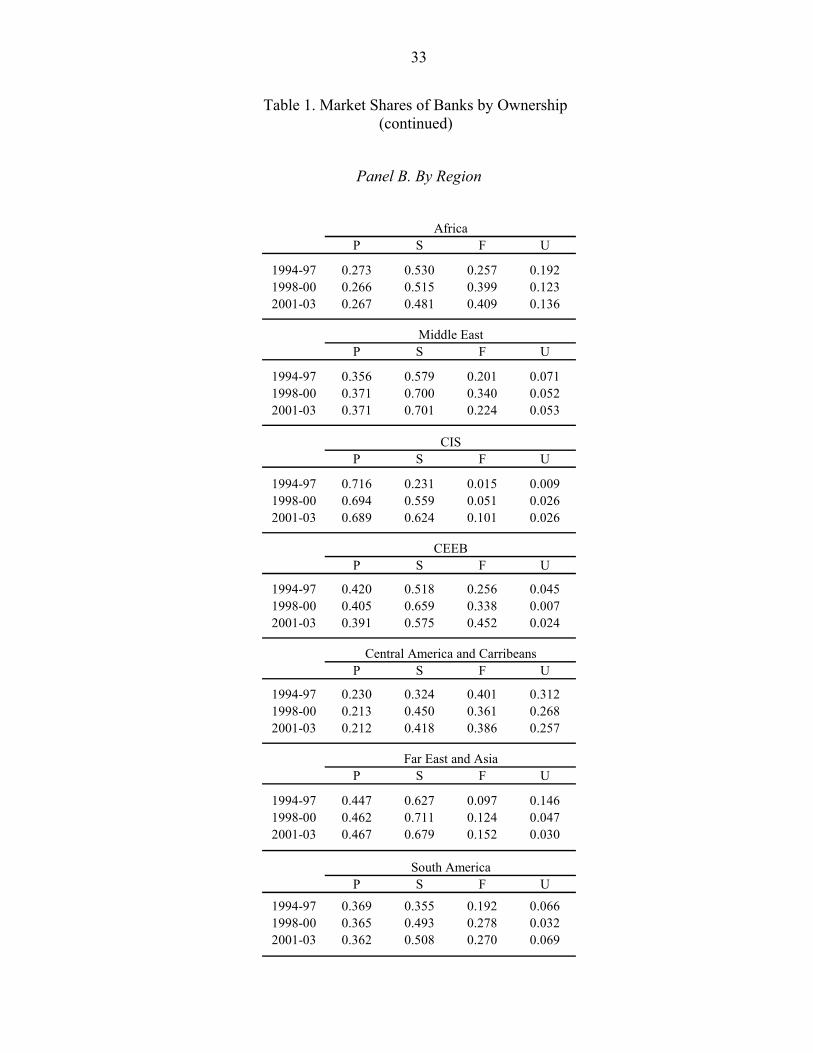
33

Table 1. Market Shares of Banks by Ownership (continued)

Panel B. By Region

P S F U

1994-97 0.273 0.530 0.257 0.1921998-00 0.266 0.515 0.399 0.1232001-03 0.267 0.481 0.409 0.136

P S F U

1994-97 0.356 0.579 0.201 0.0711998-00 0.371 0.700 0.340 0.0522001-03 0.371 0.701 0.224 0.053

P S F U

1994-97 0.716 0.231 0.015 0.0091998-00 0.694 0.559 0.051 0.0262001-03 0.689 0.624 0.101 0.026

P S F U

1994-97 0.420 0.518 0.256 0.0451998-00 0.405 0.659 0.338 0.0072001-03 0.391 0.575 0.452 0.024

P S F U

1994-97 0.230 0.324 0.401 0.3121998-00 0.213 0.450 0.361 0.2682001-03 0.212 0.418 0.386 0.257

P S F U

1994-97 0.447 0.627 0.097 0.1461998-00 0.462 0.711 0.124 0.0472001-03 0.467 0.679 0.152 0.030

P S F U

1994-97 0.369 0.355 0.192 0.0661998-00 0.365 0.493 0.278 0.0322001-03 0.362 0.508 0.270 0.069

South America

Central America and Carribeans

Far East and Asia

Africa

Middle East

CIS

CEEB

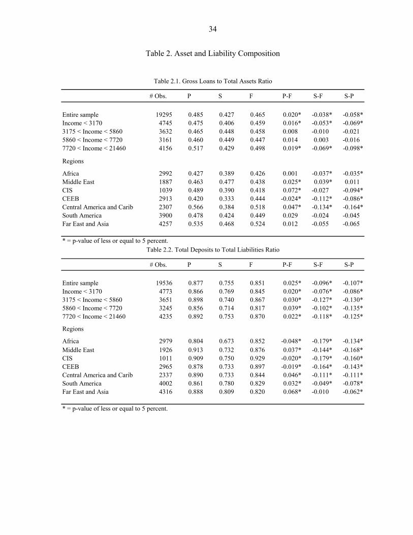
34

Table 2. Asset and Liability Composition

# Obs. P S F P-F S-F S-P

Entire sample 19295 0.485 0.427 0.465 0.020* -0.038* -0.058*Income < 3170 4745 0.475 0.406 0.459 0.016* -0.053* -0.069*3175 < Income < 5860 3632 0.465 0.448 0.458 0.008 -0.010 -0.021 5860 < Income < 7720 3161 0.460 0.449 0.447 0.014 0.003 -0.016 7720 < Income < 21460 4156 0.517 0.429 0.498 0.019* -0.069* -0.098*

Regions

Africa 2992 0.427 0.389 0.426 0.001 -0.037* -0.035*Middle East 1887 0.463 0.477 0.438 0.025* 0.039* 0.011 CIS 1039 0.489 0.390 0.418 0.072* -0.027 -0.094*CEEB 2913 0.420 0.333 0.444 -0.024* -0.112* -0.086*Central America and Carib 2307 0.566 0.384 0.518 0.047* -0.134* -0.164*South America 3900 0.478 0.424 0.449 0.029 -0.024 -0.045 Far East and Asia 4257 0.535 0.468 0.524 0.012 -0.055 -0.065

* = p-value of less or equal to 5 percent.

Table 2.1. Gross Loans to Total Assets Ratio

# Obs. P S F P-F S-F S-P

Entire sample 19536 0.877 0.755 0.851 0.025* -0.096* -0.107*Income < 3170 4773 0.866 0.769 0.845 0.020* -0.076* -0.086*3175 < Income < 5860 3651 0.898 0.740 0.867 0.030* -0.127* -0.130*5860 < Income < 7720 3245 0.856 0.714 0.817 0.039* -0.102* -0.135*7720 < Income < 21460 4235 0.892 0.753 0.870 0.022* -0.118* -0.125*

Regions

Africa 2979 0.804 0.673 0.852 -0.048* -0.179* -0.134*Middle East 1926 0.913 0.732 0.876 0.037* -0.144* -0.168*CIS 1011 0.909 0.750 0.929 -0.020* -0.179* -0.160*CEEB 2965 0.878 0.733 0.897 -0.019* -0.164* -0.143*Central America and Carib 2337 0.890 0.733 0.844 0.046* -0.111* -0.111*South America 4002 0.861 0.780 0.829 0.032* -0.049* -0.078*Far East and Asia 4316 0.888 0.809 0.820 0.068* -0.010 -0.062*

* = p-value of less or equal to 5 percent.

Table 2.2. Total Deposits to Total Liabilities Ratio

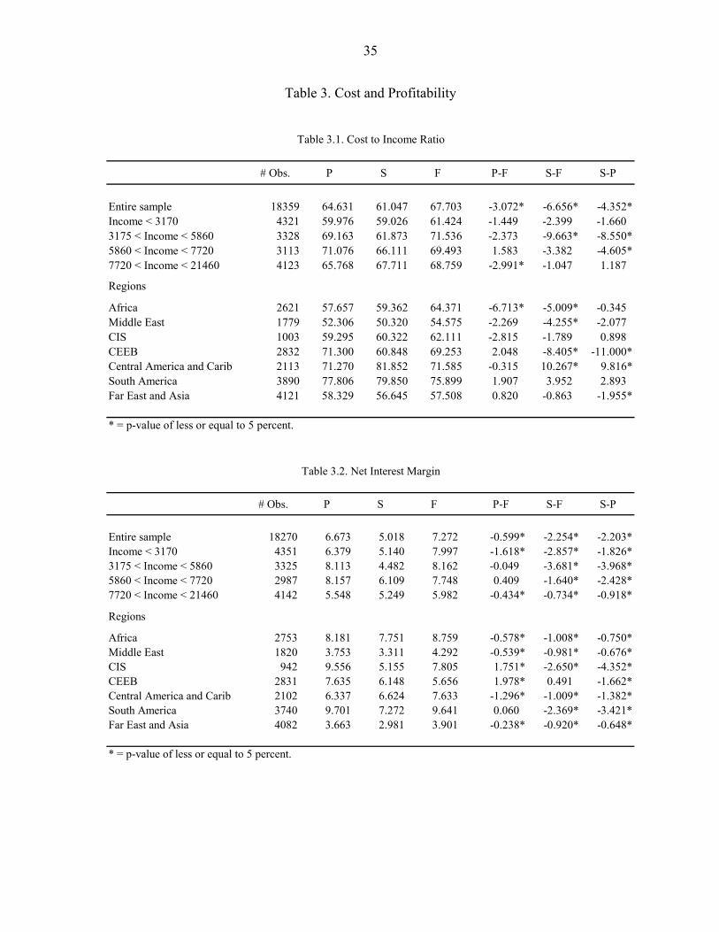
35

Table 3. Cost and Profitability

# Obs. P S F P-F S-F S-P

Entire sample 18359 64.631 61.047 67.703 -3.072* -6.656* -4.352*Income < 3170 4321 59.976 59.026 61.424 -1.449 -2.399 -1.660 3175 < Income < 5860 3328 69.163 61.873 71.536 -2.373 -9.663* -8.550*5860 < Income < 7720 3113 71.076 66.111 69.493 1.583 -3.382 -4.605*7720 < Income < 21460 4123 65.768 67.711 68.759 -2.991* -1.047 1.187

Regions

Africa 2621 57.657 59.362 64.371 -6.713* -5.009* -0.345 Middle East 1779 52.306 50.320 54.575 -2.269 -4.255* -2.077 CIS 1003 59.295 60.322 62.111 -2.815 -1.789 0.898 CEEB 2832 71.300 60.848 69.253 2.048 -8.405* -11.000*Central America and Carib 2113 71.270 81.852 71.585 -0.315 10.267* 9.816*South America 3890 77.806 79.850 75.899 1.907 3.952 2.893 Far East and Asia 4121 58.329 56.645 57.508 0.820 -0.863 -1.955*

* = p-value of less or equal to 5 percent.

Table 3.1. Cost to Income Ratio

# Obs. P S F P-F S-F S-P

Entire sample 18270 6.673 5.018 7.272 -0.599* -2.254* -2.203*Income < 3170 4351 6.379 5.140 7.997 -1.618* -2.857* -1.826*3175 < Income < 5860 3325 8.113 4.482 8.162 -0.049 -3.681* -3.968*5860 < Income < 7720 2987 8.157 6.109 7.748 0.409 -1.640* -2.428*7720 < Income < 21460 4142 5.548 5.249 5.982 -0.434* -0.734* -0.918*

Regions

Africa 2753 8.181 7.751 8.759 -0.578* -1.008* -0.750*Middle East 1820 3.753 3.311 4.292 -0.539* -0.981* -0.676*CIS 942 9.556 5.155 7.805 1.751* -2.650* -4.352*CEEB 2831 7.635 6.148 5.656 1.978* 0.491 -1.662*Central America and Carib 2102 6.337 6.624 7.633 -1.296* -1.009* -1.382*South America 3740 9.701 7.272 9.641 0.060 -2.369* -3.421*Far East and Asia 4082 3.663 2.981 3.901 -0.238* -0.920* -0.648*

* = p-value of less or equal to 5 percent.

Table 3.2. Net Interest Margin

36

Table 3. Cost and Profitability (continued)

# Obs. P S F P-F S-F S-P

Entire sample 19425 1.455 1.052 1.280 0.174* -0.228* -0.404*Income < 3170 4698 1.690 1.286 1.681 0.009 -0.395* -0.345*3175 < Income < 5860 3456 1.387 0.945 1.366 0.020 -0.421* -0.364*5860 < Income < 7720 3243 1.328 0.964 1.369 -0.041 -0.406* -0.449*7720 < Income < 21460 4361 1.137 0.502 0.721 0.416* -0.219 -0.620*

Regions

Africa 3010 2.916 2.115 2.013 0.903* 0.102 -0.406*Middle East 1904 1.454 1.367 1.776 -0.323* -0.409* -0.249*CIS 1006 2.344 2.142 2.430 -0.086 -0.288 -0.173 CEEB 2912 0.915 1.057 0.886 0.029 0.171 0.151 Central America and Carib 2209 1.229 0.055 1.171 0.059 -1.116* -1.201*South America 4007 1.392 0.229 1.021 0.371* -0.792* -1.217*Far East and Asia 4377 0.977 0.729 0.875 0.101 -0.146 -0.208*

* = p-value of less or equal to 5 percent.

Table 3.3. Return on Average Assets

# Obs. P S F P-F S-F S-P

Entire sample 19356 11.531 11.458 11.432 0.099 0.026 -0.027 Income < 3170 4616 16.101 16.169 16.697 -0.596 -0.528 0.927 3175 < Income < 5860 3479 12.671 10.568 12.708 -0.037 -2.140* -1.880 5860 < Income < 7720 3236 10.473 6.638 10.652 -0.179 -4.014* -3.896*7720 < Income < 21460 4344 6.477 5.294 5.786 0.691 -0.492 -0.782

Regions

Africa 2993 22.379 16.753 18.856 3.524* -2.103 -2.859*Middle East 1886 12.694 11.877 13.059 -0.365 -1.182 -1.072 CIS 1011 15.516 20.138 12.199 3.317 7.939* 5.172 CEEB 2872 8.688 10.269 9.890 -1.202 0.379 1.415 Central America and Carib 2236 11.807 11.198 13.025 -1.218 -1.827 -1.168 South America 4044 9.210 3.000 6.089 3.121* -3.089 -5.981*Far East and Asia 4314 8.485 11.785 9.525 -1.040 2.260* 3.648*

* = p-value of less or equal to 5 percent.

Table 3.4. Return on Average Equity

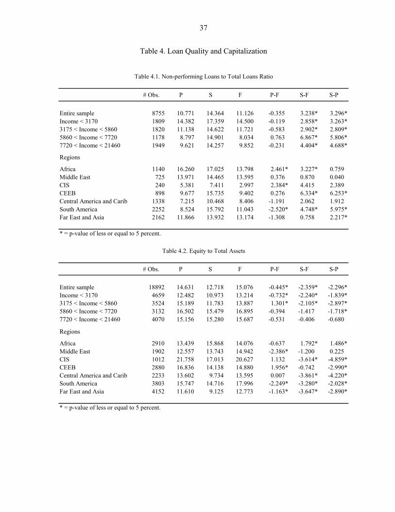
37

Table 4. Loan Quality and Capitalization

# Obs. P S F P-F S-F S-P

Entire sample 8755 10.771 14.364 11.126 -0.355 3.238* 3.296*Income < 3170 1809 14.382 17.359 14.500 -0.119 2.858* 3.263*3175 < Income < 5860 1820 11.138 14.622 11.721 -0.583 2.902* 2.809*5860 < Income < 7720 1178 8.797 14.901 8.034 0.763 6.867* 5.806*7720 < Income < 21460 1949 9.621 14.257 9.852 -0.231 4.404* 4.688*

Regions

Africa 1140 16.260 17.025 13.798 2.461* 3.227* 0.759 Middle East 725 13.971 14.465 13.595 0.376 0.870 0.040 CIS 240 5.381 7.411 2.997 2.384* 4.415 2.389 CEEB 898 9.677 15.735 9.402 0.276 6.334* 6.253*Central America and Carib 1338 7.215 10.468 8.406 -1.191 2.062 1.912 South America 2252 8.524 15.792 11.043 -2.520* 4.748* 5.975*Far East and Asia 2162 11.866 13.932 13.174 -1.308 0.758 2.217*

* = p-value of less or equal to 5 percent.

Table 4.1. Non-performing Loans to Total Loans Ratio

# Obs. P S F P-F S-F S-P

Entire sample 18892 14.631 12.718 15.076 -0.445* -2.359* -2.296*Income < 3170 4659 12.482 10.973 13.214 -0.732* -2.240* -1.839*3175 < Income < 5860 3524 15.189 11.783 13.887 1.301* -2.105* -2.897*5860 < Income < 7720 3132 16.502 15.479 16.895 -0.394 -1.417 -1.718*7720 < Income < 21460 4070 15.156 15.280 15.687 -0.531 -0.406 -0.680

Regions

Africa 2910 13.439 15.868 14.076 -0.637 1.792* 1.486*Middle East 1902 12.557 13.743 14.942 -2.386* -1.200 0.225 CIS 1012 21.758 17.013 20.627 1.132 -3.614* -4.859*CEEB 2880 16.836 14.138 14.880 1.956* -0.742 -2.990*Central America and Carib 2233 13.602 9.734 13.595 0.007 -3.861* -4.220*South America 3803 15.747 14.716 17.996 -2.249* -3.280* -2.028*Far East and Asia 4152 11.610 9.125 12.773 -1.163* -3.647* -2.890*

* = p-value of less or equal to 5 percent.

Table 4.2. Equity to Total Assets

38

Table 5. Description of Variables

Bank Variables Z(t) Z-score measure for bank risk, ( ) ( )/t t t tZ ROA EQTA ROAσ= + ROA(t) Return on average assets Log[σ(ROA(t))] ( ) 1

t t ttROA ROA T ROAσ −= − ∑

EQTA(t) Equity-to-asset ratio LEQTA(t) ( /(1 ))t t tLEQTA Ln EQTA EQTA= − GTLA(t) Gross loan-to-asset ratio LGTLA(t) ( /(1 ))t t tLGLTA Ln GLTA GLTA= − DEPL(t) Deposit-to-liabilities ratio LDEPL(t) ( /(1 ))t t tLDEPL Ln DEPL DEPL= − LASSETS(t) Log of total assets CIR(t) Cost to income ratio Market Structure SD State-owned banks dummy SF Foreign banks dummy Share2(t) Square asset market share of bank i ( )2

ijtS HHI(t) Hirschmann-Hirfendahl Index, ( 2

jt ijtiHHI S≡∑ )

HHIC(t) Hirschmann-Hirfendahl Index of bank i ’s competitors

( )2 2ijt mit jt ijtm i

HHIC S HHI S≠

≡ = −∑ .

Share2(I)(t) Square asset market share of type I bank (private domestic bank if I=P, state-owned bank if I=S, foreign bank if I=F)

HHIC(I,J)(t) HHI of all type J competitors of a type I bank, with I,J ∈ {P,S,F} HHIU(t) HHI of banks of unidentified ownership Macro Variables GDPPC(t) Per-capita GDP at PPP GROWTH(t) Real GDP Growth INFL(t) Average CPI Inflation Rate ER(t) Domestic currency/US$ exchange rate GROWTHV(t) Real GDP Growth Volatility,

1 2( )t t ttGROWTHV GROWTH T GROWTH−= − ∑

INFLV(t) Inflation Volatility, 1 2( )t t ttINFLV INFL T INFL−= − ∑

ERV(t) Exchange Rate Volatility, 1 2( )t t ttERV ER T ER−= − ∑

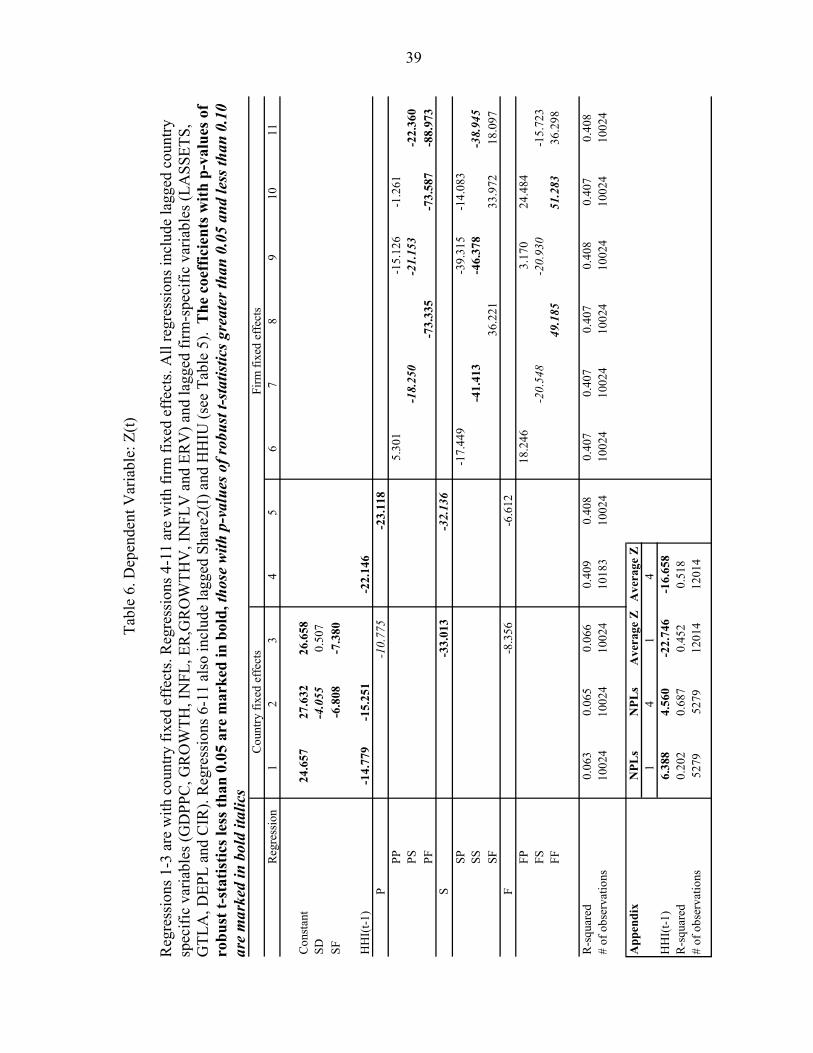
39

Tabl

e 6.

Dep

ende

nt V

aria

ble:

Z(t)

Reg

ress

ions

1-3

are

with

cou

ntry

fixe

d ef

fect

s. R

egre

ssio

ns 4

-11

are

with

firm

fixe

d ef

fect

s. A

ll re

gres

sion

s inc

lude

lagg

ed c

ount

ry

spec

ific

varia

bles

(GD

PPC

, GR

OW

TH, I

NFL

, ER

,GR

OW

THV

, IN

FLV

and

ER

V) a

nd la

gged

firm

-spe

cific

var

iabl

es (L

ASS

ETS,

G

TLA

, DEP

L an

d C

IR).

Reg

ress

ions

6-1

1 al

so in

clud

e la

gged

Sha

re2(

I) a

nd H

HIU

(see

Tab

le 5

). T

he c

oeff

icie

nts w

ith p

-val

ues o

f ro

bust

t-st

atis

tics l

ess t

han

0.05

are

mar

ked

in b

old,

thos

e w

ith p

-val

ues o

f rob

ust t

-sta

tistic

s gre

ater

than

0.0

5 an

d le

ss th

an 0

.10

ar

e m

arke

d in

bol

d ita

lics

Reg

ress

ion

12

34

56

78

910

11

Con

stan

t24

.657

27.6

3226

.658

SD-4

.055

0.50

7SF

-6.8

08-7

.380

HH

I(t-1

)-1

4.77

9-1

5.25

1-2

2.14

6P

-10.

775

-23.

118

PP5.

301

-15.

126

-1.2

61PS

-18.

250

-21.

153

-22.

360

PF-7

3.33

5-7

3.58

7-8

8.97

3S

-33.

013

-32.

136

SP-1

7.44

9-3

9.31

5-1

4.08

3SS

-41.

413

-46.

378

-38.

945

SF36

.221

33.9

7218

.097

F-8

.356

-6.6

12FP

18.2

463.

170

24.4

84FS

-20.

548

-20.

930

-15.

723

FF49

.185

51.2

8336

.298

R-s

quar

ed0.

063

0.06

50.

066

0.40

90.

408

0.40

70.

407

0.40

70.

408

0.40

70.

408

# of

obs

erva

tions

1002

410

024

1002

410

183

1002

410

024

1002

410

024

1002

410

024

1002

4

App

endi

x

NPL

sN

PLs

Ave

rage

ZA

vera

ge Z

1

41

4H

HI(

t-1)

6.38

84.

560

-22.

746

-16.

658

R-s

quar

ed0.

202

0.68

70.

452

0.51

8#

of o

bser

vatio

ns52

7952

7912

014

1201

4

Cou

ntry

fixe

d ef

fect

sFi

rm fi

xed

effe

cts

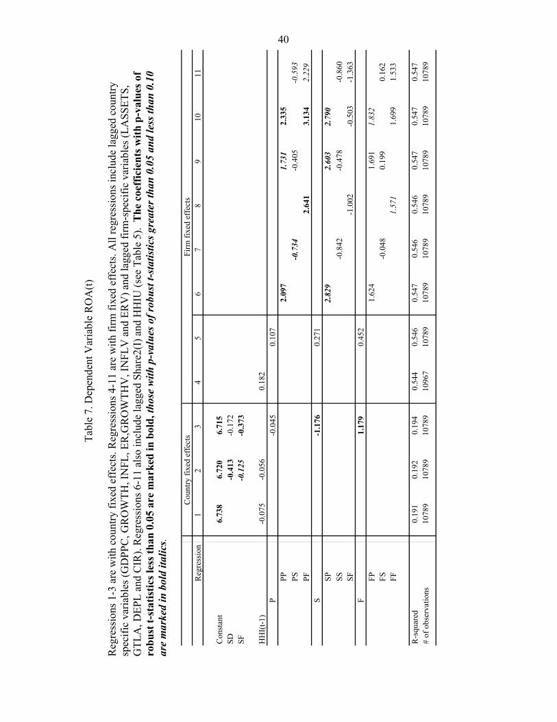
40

Tabl

e 7.

Dep

ende

nt V

aria

ble

RO

A(t)

Reg

ress

ions

1-3

are

with

cou

ntry

fixe

d ef

fect

s. R

egre

ssio

ns 4

-11

are

with

firm

fixe

d ef

fect

s. A

ll re

gres

sion

s inc

lude

lagg

ed c

ount

ry

spec

ific

varia

bles

(GD

PPC

, GR

OW

TH, I

NFL

, ER

,GR

OW

THV

, IN

FLV

and

ER

V) a

nd la

gged

firm

-spe

cific

var

iabl

es (L

ASS

ETS,

G

TLA

, DEP

L an

d C

IR).

Reg

ress

ions

6-1

1 al

so in

clud

e la

gged

Sha

re2(

I) a

nd H

HIU

(see

Tab

le 5

). T

he c

oeff

icie

nts w

ith p

-val

ues o

f ro

bust

t-st

atis

tics l

ess t

han

0.05

are

mar

ked

in b

old,

thos

e w

ith p

-val

ues o

f rob

ust t

-sta

tistic

s gre

ater

than

0.0

5 an

d le

ss th

an 0

.10

ar

e m

arke

d in

bol

d ita

lics.

Reg

ress

ion

1 2

34

56

78

910

11

Con

stan

t 6.

738

6.72

06.

715

SD

-0.4

13-0

.172

SF

-0.1

25-0

.373

HH

I(t-1

) -0

.075

-0.0

560.

182

P -0

.045

0.10

7PP

2.

097

1.73

12.

335

PS

-0.7

34-0

.405

-0.5

93PF

2.

641

3.13

42.

229

S -1

.176

0.27

1SP

2.

829

2.60

32.

790

SS

-0.8

42-0

.478

-0.8

60SF

-1

.002

-0.5

03-1

.363

F 1.

179

0.45

2FP

1.

624

1.69

11.

832

FS

-0.0

480.

199

0.16

2FF

1.

571

1.69

91.

533

R-s

quar

ed

0.19

1 0.

192

0.19

40.

544

0.54

60.

547

0.54

60.

546

0.54

70.

547

0.54

7#

of o

bser

vatio

ns

1078

9 10

789

1078

910

967

1078

910

789

1078

910

789

1078

910

789

1078

9

Cou

ntry

fixe

d ef

fect

sFi

rm fi

xed

effe

cts

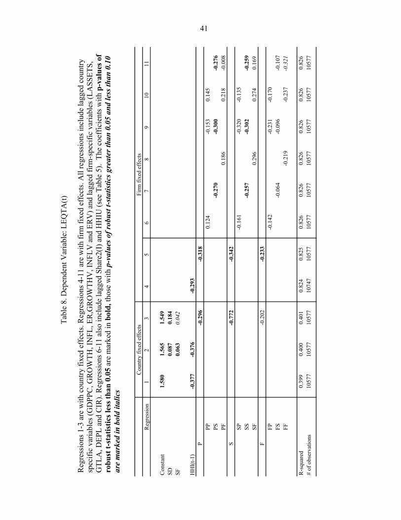
41

Tabl

e 8.

Dep

ende

nt V

aria

ble:

LEQ

TA(t)

Reg

ress

ions

1-3

are

with

cou

ntry

fixe

d ef

fect

s. R

egre

ssio

ns 4

-11

are

with

firm

fixe

d ef

fect

s. A

ll re

gres

sion

s inc

lude

lagg

ed c

ount

ry

spec

ific

varia

bles

(GD

PPC

, GR

OW

TH, I

NFL

, ER

,GR

OW

THV

, IN

FLV

and

ER

V) a

nd la

gged

firm

-spe

cific

var

iabl

es (L

ASS

ETS,

G

TLA

, DEP

L an

d C

IR).

Reg

ress

ions

6-1

1 al

so in

clud

e la

gged

Sha

re2(

I) a

nd H

HIU

(see

Tab

le 5

). T

he c

oeff

icie

nts w

ith p

-val

ues o

f ro

bust

t-st

atis

tics l

ess t

han

0.05

are

mar

ked

in b

old,

thos

e w

ith p

-val

ues o

f rob

ust t

-sta

tistic

s gre

ater

than

0.0

5 an

d le

ss th

an 0

.10

ar

e m

arke

d in

bol

d ita

lics

Reg

ress

ion

1 2

34

56

78

910

11

Con

stan

t 1.

580

1.56

51.

549

SD

0.08

70.

184

SF

0.06

30.

042

HH

I(t-1

) -0

.377

-0

.376

-0.2

93P

-0.2

96-0

.318

PP

0.12

4 -0

.153

0.14

5PS

-0

.270

-0.3

00-0

.276

PF

0.18

60.

218

-0.0

08S

-0.7

72-0

.342

SP

-0.1

61

-0.3

20-0

.135

SS

-0.2

57-0

.302

-0.2

59SF

0.

296

0.27

40.

169

F -0

.202

-0.2

33FP

-0

.142

-0

.231

-0.1

70FS

-0

.064

-0.0

96-0

.107

FF

-0.2

19-0

.237

-0.3

21

R-s

quar

ed

0.39

9 0.

400

0.40

10.

824

0.82

50.

826

0.82

60.

826

0.82

60.

826

0.82

6#

of o

bser

vatio

ns

1057

7 10

577

1057

710

747

1057

710

577

1057

710

577

1057

710

577

1057

7

Cou

ntry

fixe

d ef

fect

sFi

rm fi

xed

effe

cts

42

Tabl

e 9.

Dep

ende

nt V

aria

ble:

Ln[

((

))RO

At

σ]

Reg

ress

ions

1-3

are

with

cou

ntry

fixe

d ef

fect

s. R

egre

ssio

ns 4

-11

are

with

firm

fixe

d ef

fect

s. A

ll re

gres

sion

s inc

lude

lagg

ed c

ount

ry

spec

ific

varia

bles

(GD

PPC

, GR

OW

TH, I

NFL

, ER

,GR

OW

THV

, IN

FLV

and

ER

V) a

nd la

gged

firm

-spe

cific

var

iabl

es (L

ASS

ETS,

G

TLA

, DEP

L an

d C

IR).

Reg

ress

ions

6-1

1 al

so in

clud

e la

gged

Sha

re2(

I) a

nd H

HIU

(see

Tab

le 5

). Th

e co

effic

ient

s with

p-v

alue

s of

robu

st t-

stat

istic

s les

s tha

n 0.

05 a

re m

arke

d in

bol

d, th

ose

with

p-v

alue

s of r

obus

t t-s

tatis

tics g

reat

er th

an 0

.05

and

less

than

0.1

0

are

mar

ked

in b

old

italic

s

Reg

ress

ion

12

34

56

78

910

11

Con

stan

t3.

074

3.01

03.

050

SD0.

169

0.12

7SF

0.17

50.

059

HH

I(t-1

)0.

300

0.30

70.

064

P0.

121

0.08

6PP

-0.0

050.

166

0.04

7PS

0.12

40.

158

0.14

6PF

0.55

70.

567

0.67

1S

0.35

4-0

.132

SP-0

.072

0.13

9-0

.241

SS0.

368

0.39

80.

238

SF-1

.714

-1.7

49-1

.568

F0.

707

0.11

4FP

0.30

50.

666

0.17

6FS

0.50

40.

582

0.38

0FF

-1.0

57-1

.043

-0.8

27

R-s

quar

ed0.

180

0.18

30.

183

0.59

10.

592

0.59

30.

593

0.59

30.

593

0.59

30.

593

# of

obs

erva

tions

1078

010

780

1078

010

958

1078

010

780

1078

010

780

1078

010

780

1078

0

Cou

ntry

fixe

d ef

fect

sFi

rm fi

xed

effe

cts

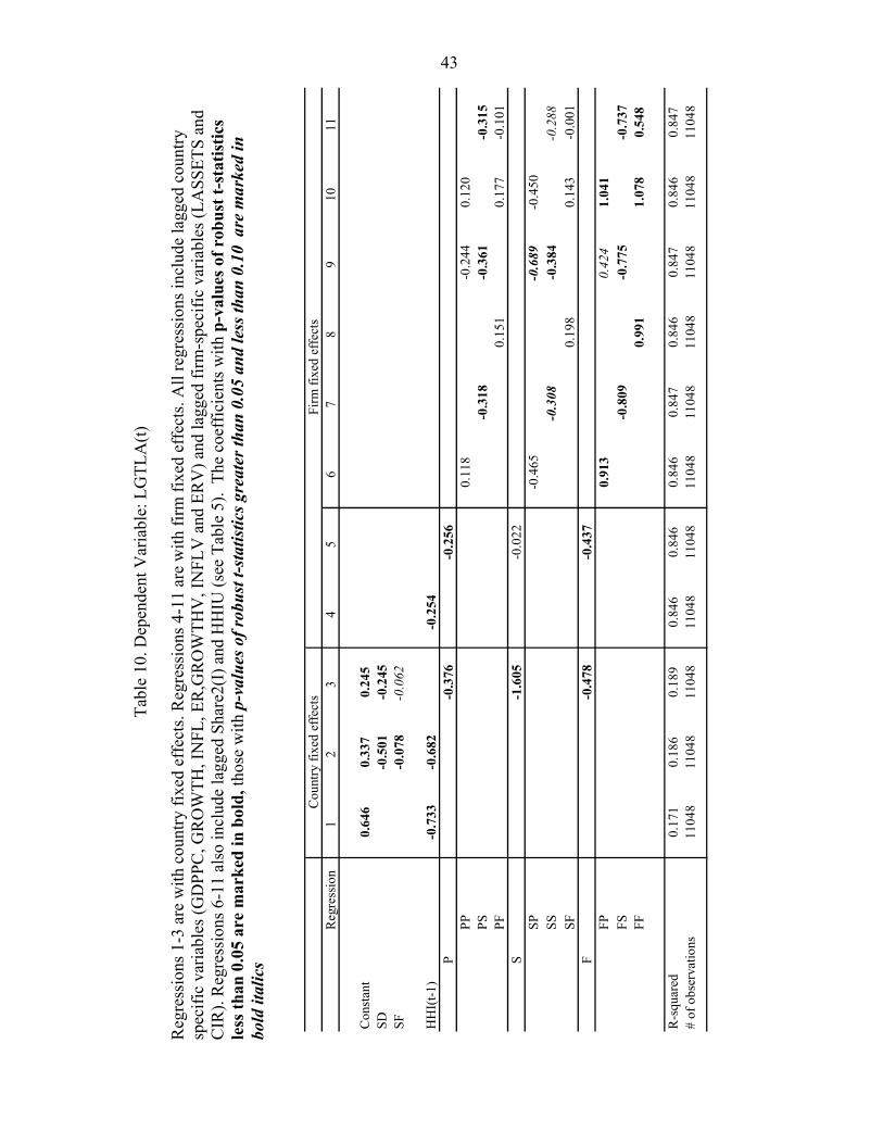
43

Tabl

e 10

. Dep

ende

nt V

aria

ble:

LG

TLA

(t)

Reg

ress

ions

1-3

are

with

cou

ntry

fixe

d ef

fect

s. R

egre

ssio

ns 4

-11

are

with

firm

fixe

d ef

fect

s. A

ll re

gres

sion

s inc

lude

lagg

ed c

ount

ry

spec

ific

varia

bles

(GD

PPC

, GR

OW

TH, I

NFL

, ER

,GR

OW

THV

, IN

FLV

and

ER

V) a

nd la

gged

firm

-spe

cific

var

iabl

es (L

ASS

ETS

and

CIR

). R

egre

ssio

ns 6

-11

also

incl

ude

lagg

ed S

hare

2(I)

and

HH

IU (s

ee T

able

5).

The

coe

ffic

ient

s with

p-v

alue

s of r

obus

t t-s

tatis

tics

less

than

0.0

5 ar

e m

arke

d in

bol

d, th

ose

with

p-v

alue

s of r

obus

t t-s

tatis

tics g

reat

er th

an 0

.05

and

less

than

0.1

0 a

re m

arke

d in

bo

ld it

alic

s

Reg

ress

ion

12

34

56

78

910

11

Con

stan

t0.

646

0.33

70.

245

SD-0

.501

-0.2

45SF

-0.0

78-0

.062

HH

I(t-1

)-0

.733

-0.6

82-0

.254

P-0

.376

-0.2

56PP

0.11

8-0

.244

0.12

0PS

-0.3

18-0

.361

-0.3

15PF

0.15

10.

177

-0.1

01S

-1.6

05-0

.022

SP-0

.465

-0.6

89-0

.450

SS-0

.308

-0.3

84-0

.288

SF0.

198

0.14

3-0

.001

F-0

.478

-0.4

37FP

0.91

30.

424

1.04

1FS

-0.8

09-0

.775

-0.7

37FF

0.99

11.

078

0.54

8

R-s

quar

ed0.

171

0.18

60.

189

0.84

60.

846

0.84

60.

847

0.84

60.

847

0.84

60.

847

# of

obs

erva

tions

1104

811

048

1104

811

048

1104

811

048

1104

811

048

1104

811

048

1104

8

Cou

ntry

fixe

d ef

fect

sFi

rm fi

xed

effe

cts

44

Tabl

e 11

. Dep

ende

nt V

aria

ble:

LD

EPL(

t)

Reg

ress

ions

1-3

are

with

cou

ntry

fixe

d ef

fect

s. R

egre

ssio

ns 4

-11

are

with

firm

fixe

d ef

fect

s. A

ll re

gres

sion

s inc

lude

lagg

ed c

ount

ry

spec

ific

varia

bles

(GD

PPC

, GR

OW

TH, I

NFL

, ER

,GR

OW

THV

, IN

FLV

and

ER

V) a

nd la

gged

firm

-spe

cific

var

iabl

es (L

ASS

ETS

and

CIR

). R

egre

ssio

ns 6

-11

also

incl

ude

lagg

ed S

hare

2(I)

and

HH

IU (s

ee T

able

5).

The

coe

ffic

ient

s with

p-v

alue

s of r

obus

t t-s

tatis

tics

less

than

0.0

5 ar

e m

arke

d in

bol

d, th

ose

with

p-v

alue

s of r

obus

t t-s

tatis

tics g

reat

er th

an 0

.05

and

less

than

0.1

0 a

re m

arke

d in

bo

ld it

alic

s.

Regr

essio

n1

23

45

67

89

1011

Cons

tant

2.62

82.

069

2.01

0SD

-0.8

53-0

.692

SF-0

.090

-0.0

72

HHI(t

-1)

-0.4

77-0

.402

-0.1

77P

-0.1

96-0

.018

PP-0

.435

-0.4

28-0

.512

PS0.

094

0.02

00.

047

PF-0

.798

-0.9

03-0

.774

S-0

.976

-0.5

98SP

-0.0

73-0

.224

-0.2

10SS

-0.2

96-0

.323

-0.3

99SF

-1.2

80-1

.314

-1.4

54F

-0.2

99-0

.149

FP0.

506

0.40

70.

493

FS-0

.188

-0.1

56-0

.237

FF-0

.100

-0.0

49-0

.247

R-sq

uare

d0.

201

0.23

20.

233

0.78

60.

786

0.78

60.

786

0.78

70.

786

0.78

70.

787

# of

obs

erva

tions

1119

711

197

1119

711

197

1119

711

197

1119

711

197

1119

711

197

1119

7

Coun

try fi

xed

effe

ctsFi

rm fi

xed

effe

cts