Banking Reform in India M - Brookings Institution · Banking Reform in India M ... sector bank we...

A B H I J I T V . B A N E R J E EMassachusetts Institute of Technology

S H A W N C O L EMassachusetts Institute of Technology

E S T H E R D U F L OMassachusetts Institute of Technology

Banking Reform in India

Measured by share of deposits, 83 percent of the banking businessin India is in the hands of state or nationalized banks, banks

owned by the government in some increasingly less clear-cut way. More-over, even non-nationalized banks are subject to extensive regulationson whom they can lend to, in addition to the more standard prudentialregulations.

Government control over banks has always had its fans, ranging fromLenin to Gerschenkron. Although some advocates have emphasized thepolitical importance of public control over banking, most arguments fornationalizing banks are based on the premise that profit-maximizing lend-ers do not necessarily deliver credit where the social returns are highest.The Indian government, when nationalizing all the larger Indian banks in1969, argued that banking was “inspired by a larger social purpose” andmust “subserve national priorities and objectives such as rapid growth inagriculture, small industry and exports.”1

A body of direct and indirect evidence now shows that credit markets indeveloping countries often fail to deliver credit where its social productmight be the highest, and both agriculture and small industry are often men-tioned as sectors that do not get their fair share of credit.2 If nationalization

277

We thank the Reserve Bank of India, in particular Y. V. Reddy, R. B. Barman, andAbhiman Das, for generous assistance with technical and substantive issues. We also thankAbhiman Das for performing calculations that involved proprietary RBI data and SaibalGhosh and Petia Topalova for helpful comments. We are grateful to the staff of the publicsector bank we study for allowing us access to their data. We gratefully acknowledgefinancial support from the Alfred P. Sloan Foundation.

1. From the “Bank Company Acquisition Act of 1969.” Quoted by Burgess and Pande(2003).

2. See Banerjee (2003) for a review of the evidence.

2409-07_Banerjee.qxd 12/8/04 1:36 PM Page 277

succeeds in pushing credit into these sectors, as the Indian governmentclaimed it would, it could indeed raise both equity and efficiency.

The cross-country evidence on the impact of bank nationalization, how-ever, is not encouraging. For example, Rafael La Porta and colleagues findin a cross-country setting that government ownership of banks is negativelycorrelated with both financial development and economic growth.3 Theyinterpret this as support for their view that the potential benefits of publicownership of banks, and public control over banks more generally, areswamped by the costs that come from the agency problems it creates—problems such as cronyism, which leads to the deliberate misallocation ofcapital; bureaucratic lethargy, which leads to less deliberate but perhapsequally costly errors in the allocation of capital; and inefficiency in mobi-lizing savings and transforming them into credit.

Interpreting this type of cross-country analysis is never easy, especiallyin the case of something like bank nationalization, which is typically partof a package of other policies. Microeconomic studies of the effect of banknationalization are rare. One exception is Atif Mian’s examination of the1991 privatization of a large public bank in Pakistan.4 He finds that the pri-vatized bank did a better job both at choosing profitable clients and moni-toring existing clients than the commercial banks that remained public.Studying a liberalization episode in France, Marianne Bertrand and col-leagues find that after deregulation banks responded more to profitabilitywhen making lending decisions, and that borrowing firms were more likelyto exit or restructure following a negative shock.5

In a 2003 paper we used micro data from a nationalized bank to evalu-ate the effectiveness of the Indian banking system in delivering credit.6 Ourconclusion was that the Indian financial system is characterized by under-lending in the sense that many firms could earn large profits if they weregiven access to credit at the current market prices.

This paper builds on previous work of our own and of others to assess therole of the Indian government in the banking sector. We begin by providinga brief history of banking in India. Next we investigate the quality of inter-mediation. We first present evidence of substantial under-lending in India.To understand what role public ownership of banks may play in under-lending, we identify differences between public and private banks in thesectoral allocation of credit. In particular, we focus on whether being

278 INDIA POLICY FORUM, 2004

3. La Porta, Lopez-de-Silanes, and Shleifer (2002).4. Mian (2000).5. Bertrand, Schoar, and Thesmar (2003).6. Banerjee, Cole, and Duflo (2003).


nationalized has made these banks more responsive to what the Indian gov-ernment wants them to do. We report results, based on work by ShawnCole, showing that on many of the declared objectives of “social banking,”with the exception of agricultural lending, the private banks were no lessresponsive than the comparable nationalized banks.7 And we comparethe performance of public and private banks as financial intermediariesand conclude that the public banks have been less aggressive than privatebanks in lending, in attracting deposits, and in setting up branches, at leastsince 1990.

To understand under-lending, we dig deeper into the lending processesof nationalized banks and find that official lending policy is very rigid.Moreover, loan officers do not appear to use what little flexibility theyhave. Bankers in the public sector appear to have a preference for what wemay call passive lending. To understand why, we examine the incentivesand constraints faced by public loan officers. We focus on whether vigi-lance activity impedes lending and whether public sector banks prefer tolend to the government, rather than private firms.

Next we compare the performance of public and private banking in twoother areas. First, we examine how nationalization of banks has affected theavailability of bank branches in rural areas and find that, if anything,nationalization appears to have inhibited the growth of rural branches.Second, we address the sensitive issue of nonperforming assets andbailouts. While the data set we have now is rather sparse, it appears that thebailouts of the public banks have proved more expensive for the govern-ment, but once we control for differences in size between the public andprivate banks, this conclusion is less clear-cut.

We conclude with a short discussion of the implications of these resultsfor the future of banking reform.

Background

India has a long history of both public and private banking. Modern bank-ing in India began in the eighteenth century, with the founding of theEnglish Agency House in Calcutta and Bombay. In the first half of thenine-teenth century, three presidency banks were founded. After the 1860 intro-duction of limited liability, private banks began to appear, and foreignbanks entered the market. The beginning of the twentieth century saw the

Abhijit V. Banerjee, Shawn Cole, and Esther Duflo 279

7. Cole (2004).


introduction of joint stock banks. In 1935 the presidency banks weremerged to form the Imperial Bank of India, subsequently renamed the StateBank of India. That same year, India’s central bank, the Reserve Bank ofIndia (RBI), began operation. Following independence, the RBI was givenbroad regulatory authority over commercial banks in India. In 1959 theState Bank of India acquired the state-owned banks of eight former princelystates. Thus, by July 1969, approximately 31 percent of scheduled bankbranches throughout India were government-controlled as part of the StateBank of India.

India’s postwar development strategy was in many ways a socialist one,and the government felt that banks in private hands did not lend enough tothose who needed it most. In July 1969, the government nationalized allbanks whose nationwide deposits were greater than Rs. 500 million, nation-alizing 54 percent more of the branches in India and bringing the total shareof branches under government control to 84 percent.

Prakesh Tandon, a former chairman of the Punjab National Bank(nationalized in 1969) describes the rationale for nationalization as follows:

Many bank failures and crises over two centuries, and the damage they didunder “laissez faire” conditions; the needs of planned growth and equitable dis-tribution of credit, which in privately owned banks was concentrated mainly onthe controlling industrial houses and influential borrowers; the needs of grow-ing small-scale industry and farming regarding finance, equipment and inputs;from all these there emerged an inexorable demand for banking legislation,some government control and a central banking authority, adding up, in the finalanalysis, to social control and nationalization.8

After nationalization, the Indian banking sector expanded in breadth andscope at a rate perhaps unmatched by any other country. Indian banking hasbeen remarkably successful at achieving mass participation. Since the 1969nationalizations, more than 58,000 bank branches have opened in India.As of March 2003, these new branches had mobilized more than Rs. 9 tril-lion in deposits, the overwhelming majority of deposits in Indian banks.9

This rapid expansion is attributable to a policy requiring banks to openfour branches in unbanked locations for every branch opened in bankedlocations.

Between 1969 and 1980, private branches grew more quickly in numberthan public banks, and on April 1, 1980, they accounted for approximately17.5 percent of bank branches in India. In April 1980, the governmentundertook a second round of nationalization, placing under its control the


8. Tandon (1989, p. 198).9. Reserve Bank of India, Statistical Tables Relating to Banks in India (2003).


six private banks whose nationwide deposits were above Rs. 2 billion, or afurther 8 percent of bank branches, leaving approximately 10 percent ofbank branches in private hands. That share stayed fairly constant between1980 and 2000.

Nationalized banks remained corporate entities, retaining most of theirstaff, with the exception of the boards of directors, who were replaced byappointees of the central government. The political appointments includedrepresentatives from the government, industry, and agriculture, as well asthe public. (Equity holders in the national bank were reimbursed at approx-imately par.)

Since 1980, there has been no further nationalization, and indeedthe trend appears to be reversing itself, as nationalized banks are issuingshares to the public in what amounts to a step toward privatization. Theconsiderable accomplishments of the Indian banking sector notwithstand-ing, advocates for privatization argue that privatization will lead to severalsubstantial improvements.

Recently, the Indian banking sector has witnessed the introduction ofseveral “new private banks,” either newly founded or created by existingfinancial institutions. The new private banks have grown quickly in the pastfew years, and one is now the nation’s second largest bank. India has alsoseen the entry of more than two dozen foreign banks since the commence-ment of financial reforms in1991. Although we believe both these types ofbanks deserve study, our focus here is on the older private sector and onnationalized banks, because they represent the overwhelming majority ofbanking activity in India.

The Indian banking sector has historically suffered from high interme-diation costs, in no small part because of the staffing at public sector banks.As of March 2002, nationalized banks had 1.17 crore of deposits peremployee, as against 2.05 crore per employee for private sector banks. Aswith other government-run enterprises, corruption is a problem for publicsector banks. In 1999, 1,916 cases of possible corruption attracted attentionfrom the Central Vigilance Commission. Although not all these casesrepresent crimes, the investigations themselves may have a harmful effectif bank officers fear that approving any risky loan will inevitably lead toscrutiny. Advocates for privatization also criticize public sector banking asunresponsive to credit needs.

In the rest of the paper, we use recent evidence on banking in India toshed light on the relative costs and benefits of nationalized banks. Through-out this exercise, it is important to bear in mind that the Indian bankingsector is going through something like a transformation. Thus, evaluating



its performance using historical data requires caution. Nevertheless, datafrom the past are all we have, and change is not so rapid as to invalidate thelessons learned.

Quality of Intermediation

In this section, we carefully examine how credit is allocated in India. Wefocus initially on small-scale industries (SSI), because small firms typicallyturn to banks for external financing and because providing credit to this sec-tor is an important objective of Indian banking policy. Finding that smallfirms are indeed constrained, we then ask how bank nationalization hasaffected the flow of credit to small-scale industry and other sectors. Finally,we take a longer view of financial development, comparing how quicklypublic sector banks grew compared with their private counterparts.

The Problem of Under-Lending

A firm is getting too little credit if the marginal product of its capital ishigher than the rate of interest it is paying on its marginal rupee of borrow-ing. A firm’s inability to raise enough capital is a problem involving notmerely its own bank but the market as a whole. Under-lending therefore isa characteristic of the entire financial system. Although we focus in thispaper on the clients of a single public sector bank, if these firms are gettingtoo little credit from that bank, they should in theory have the option ofgoing elsewhere for more credit. If they do not or cannot exercise thisoption, the market cannot be doing what, in its idealized form, we wouldhave expected it to do.

We know, however, that the Indian financial system does not function asthe ideal credit market might. Most small or medium firms have a relation-ship with one bank, which they have built up over some time. They cannotexpect to walk into another bank and get as much credit as they want. Forthat reason, their ability to finance investments they need to make doesdepend on the willingness of that one bank to finance them. In this sense theresults we report below might very well reflect the specificities of the pub-lic sector banks, or even the one bank that was kind enough to share its datawith us, though given that it is seen as one of the best public sector banks,it seems unlikely that we would find much better results in other banks inits category. On the other hand, we do not have comparable data from anyprivate bank and therefore cannot tell whether under-lending is as much of



a problem for private banks. We will, however, later report some results onthe relative performance of public and private banks in terms of overallcredit delivery.

Our identification of credit-constrained firms is based on the followingsimple observation: if a firm that is not credit constrained is offered extracredit at a rate below what it is paying on the market, then the best way touse the new loan must be to pay down the firm’s current market borrow-ing, rather than to invest more. Because any additional investment by afirm that is not credit constrained will drive the marginal product of capi-tal below what the firm is paying on its market borrowing, it follows thatsuch a firm will expand its investment in response to the availability ofadditional subsidized credit only if it has no more market borrowing. Bycontrast, a firm that is credit constrained will always expand its investmentto some extent.

A corollary to this prediction is that for unconstrained firms, growth inrevenue should be slower than the growth in subsidized credit. This is adirect consequence of the fact that firms are substituting subsidized creditfor market borrowing. Therefore, if these growth rates are the same, thefirm must be credit constrained. Of course, revenue could increase moreslowly than credit even for nonconstrained firms, if the firm faces decliningmarginal returns to capital.

These predictions are more robust than the traditional way of measuringcredit constraints as the excess sensitivity of investment to cash flow.10 Ourapproach inscribes itself in a literature that tries to identify specific shocksto wealth in order to identify credit constraints.11

In an earlier paper, two of us (Banerjee and Duflo) tested these predic-tions by taking advantage of a recent change in the “priority sector”rules: all banks in India are required to lend at least 40 percent of their netcredit to the priority sector, which includes small-scale industry, at an inter-est rate no more than 4 percentage points above their prime lending rate.12

Banks that do not satisfy the priority sector target are required to lendmoney to specific government agencies at low rates of interest. In January1998, eligibility for inclusion in the small-scale industry category wasexpanded, and the limit on a firm’s total investment in plants and machin-ery was raised from Rs. 6.5 million to Rs. 30 million. Our empirical strat-egy focuses on the firms that became newly eligible for credit in this period;


10. See Bernanke and Gertler (1989), Fazzari, Hubbard, and Petersen (1998), and thecriticism in Kaplan and Zingales (2000).

11. See, inter alia, Blanchflower and Oswald (1998), Lamont (1997).12. Banerjee and Duflo (2003).


we use firms that were already eligible as a control. The results from ouranalysis are reported briefly below.

Data: Our data are from one of the better-performing Indian public sec-tor banks. The bank’s loan folders report on profit, sales, credit lines andutilization, and interest rates, as well as all numbers that the banker wasrequired to calculate (for example, his projection of the bank’s futureturnover and his calculation of the bank’s credit needs) in order to deter-mine the amount to be lent. We record these and will use them in the analy-sis described in the next section. We have data on 253 firms (including93 newly eligible firms); for 175 of these firms, the data are available forthe entire 1997 to 1999 period.

Specification: Through much of this section we will estimate an equa-tion of the form

(1) yit − yit−1 = αy BIGi + βy POSTt − γy BIG * POSTt + εyit,

with y taking the role of the various outcomes of interest (credit, revenue,profits, and so forth) and the dummy POST representing the post-January1998 period. We are in effect comparing how the outcomes change for thebig firms after 1998 with how they change for the small firms. Because y isalways a growth rate, this is, in effect, a triple difference. We can allowsmall firms and big firms to have different rates of growth, and the rate ofgrowth to differ from year to year, but we assume that there would havebeen no differential changes in the rate of growth of small and large firmsin 1998 absent the change in the priority sector regulation.

Using, respectively, the log of the credit limit and the log of next year’ssales (or profit) in place of y in equation 1, we obtain the first stage and thereduced form of a regression of sales on credit, using the interaction POST *BIG as an instrument for credit. We will present the corresponding instru-mental variable regressions.

Results: The change in the regulation certainly had an impact on whogot priority sector credit. The credit limit granted to firms below Rs. 6.5million in plant and machinery (henceforth, small firms) grew by 11.1 per-cent during 1997, while that granted to firms between Rs.6.5 million andRs. 30 million (henceforth, big firms) grew by 5.4 percent. In 1998, afterthe change in rules, small firms had 7.6 percent growth while the big firmshad 11.3 percent growth. In 1999, both big and small firms had about thesame growth, suggesting they had reached the new status quo.

This is confirmed when we estimate equation 1 using bank credit as theoutcome. The result is presented in column 2 of table 1 for the entire sam-ple of firms. The coefficient of the interaction term POST * BIG is 0.095,



with a standard error of 0.033. Column 1 estimates the probability that afirm’s credit limit was changed: the coefficient on POST * BIG is close tozero and insignificant, suggesting that the reform did not affect whichfirm’s limits were changed. This corresponds to the general observationsthat whether a firm’s file is brought out for a change in limit responds notto the needs of the firm, but to internal dynamics of the bank. We use thisfact to partition the sample into two groups on the basis of whether therewas a change in the credit limit: we use the sample where there was nochange in limit as a “placebo” group, where we can test our identificationassumption. Finally, column 3 gives the estimated impact of the reform onloan size for firms whose limit was changed: the coefficient of the interac-tion POST * BIG is 0.27, with a standard error of 0.10.

This increase in credit was not accompanied by a change in the rate ofinterest (column 4). It did not lead to reduction in the rate of utilization ofthe limits by the big firms (column 5): the ratio of total turnover (the sumof all debts incurred during the year) to credit limit is not associated withthe interaction POST * BIG. The additional credit limit thus resulted in anincrease in bank credit utilization by the firms.


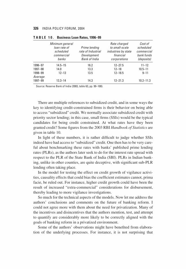
T A B L E 1 . Regressions Estimating the Effect of the 1998 Reform of Bank Regulation on Changes in Bank Credit to Firmsa

Sample and dependent variable b

Whole sample Sample with change in credit limit

Dummy for Change in Change in Change in Change in firmIndependent any change bank lending bank lending interest rate utilization of variable in limit to firm to firm to firm credit limit

POST c 0.000 −0.034 −0.115 −0.007 −0.030(0.05) (0.026) (0.074) (0.015) (0.336)

BIG d −0.043 −0.059 −0.218 −0.002 0.257(0.052) (0.028) (0.088) (0.014) (0.362)

POST * BIG −0.022 0.095 0.271 0.009 −0.128(0.087) (0.033) (0.102) (0.02) (0.458)

No. of observations 487 487 155 141 44

Source: Authors’ regressions using data on client firms of a public sector bank in India.a. Each column reports regression coefficients for a single regression using ordinary least squares.

Standard errors, corrected for heteroskedasticity and for clustering at the sectoral level, are in parentheses. b. All dependent variables (except in the first column) are calculated as differences in logarithms (for

example, the logarithm of lending in the current period minus the logarithm of lending in the previous period).c. Dummy variable taking a value of 1 when the year is 1998 or later, following the change in regula-

tion on lending to the priority sector.d. Dummy variable taking a value of 1 when the firm has plant and machinery valued at more than

Rs. 6.5 million.


Table 2 presents the impact of this increase in credit on sales and profits.The coefficient of the interaction POST * BIG in the sales equation in thesample where the limit was increased is 0.19, with a standard error of 0.11(column 1). By contrast, in the sample where there was no increase in limit,the interaction POST * BIG is close to zero (0.007) and insignificant (col-umn 1, line 2), which suggests that the sales result is not driven by a failureof the identification assumption. The coefficient of the interaction POST *BIG is 0.27 in the credit regression and 0.19 in the sales regression: thus,sales increased almost as fast as loans in response to the reform. This is anindication that there was little or no substitution of bank credit for nonbankcredit as a result of the reform and thus that firms are credit constrained.

Additional evidence is provided in column 2. We restrict the sample tofirms that have a positive amount of borrowing from the market both before


T A B L E 2 . Regressions Estimating the Effect of Priority Sector Reform on Firm Sales, Sales-to-Loans Ratios, and Profitsa

Dependent variable and sample

Change in firm sales b

Complete Sample without Change in firm Regression sample credit substitution profits b

Reduced-form estimatesSample with change in credit limit

Coefficient on POST * BIG 0.194 0.168 0.538Standard error (0.106) (0.118) (0.281)No. of observations 152 136 141

Sample with no change in credit limitCoefficient on POST * BIG 0.007 0.022 0.280Standard error (0.074) (0.081) (0.473)No. of observations 301 285 250

Whole sampleCoefficient on POST * BIG 0.071 0.071 0.316Standard error (0.068) (0.069) (0.368)No. of observations 453 421 391

Instrumental variables estimatesSample with change in credit limit

Estimate for change in lendingc 0.75 1.79Standard error (0.37) (0.94)No. of observations 152 141

Source: Authors’ regressions using data on client firms of a public sector bank in India.a. Dummy variables POST and BIG are defined as in table 1. Standard errors, corrected for het-

eroskedasticity and for clustering at the sectoral level, are in parentheses. b. Changes in sales and in profits are calculated as differences in logarithms from the previous to the

current period.c. Calculated as the difference in logarithms from the previous to the current period.


and after the reform and thus have not completely substituted bank bor-rowing for market borrowing. In this sample as well, we obtain a positiveand significant effect of the interaction POST * BIG, indicating that thesefirms must be credit constrained.

In column 3, we present the effect of the reform on profit. Because ourdependent variable is the logarithm of profit, we can estimate the impactonly on firms whose profits were positive. The effect is even bigger thanthat on sales: 0.54, with a standard error of 0.28. Here again, we see noeffect of the interaction POST * BIG in the sample without a change inlimit (line 2), which lends support to our identification assumption.

The large effect on profit is not sufficient to establish the presence ofcredit constraints: even unconstrained firms should see profits increasewhen they gain access to subsidized credit, because they would substitutecheaper capital for more expensive capital. However, if firms were notexpanding, we should not expect to see sales (column 1) or costs (notreported) expand as well.

The instrumental variable (IV) estimate of the effect of loans on salesand profit implied by the reduced form and first stage estimates in columns1 and 3 are presented in the bottom panel of table 2. Note that the coeffi-cient in column 1 is a lower bound of the effect of working capital on sales,because the reform should have led to some substitution of bank credit formarket credit. The IV coefficient is 0.75, with a standard error of 0.37. Theeffect of working capital on sales is very close to 1, a result that wouldimply that there cannot be an equilibrium without credit constraint.

The IV estimate of the impact of bank credit on profit is 1.79, thoughagain the sample is limited to firms with positive profits. The estimate issubstantially greater than 1, which suggests that the technology has a strongfixed-cost component. However, these coefficients also allow us to esti-mate the effect of credit expansion on profits.

We can use this estimate to get a sense of the average increase in profitcaused by every rupee in loan. The average loan is Rs. 86,800. Therefore anincrease of Rs. 1,000 in the loan corresponds to a 1.15 percent increase inloans. Taking 1.79 as the estimate of the effect of the log increase in loan onlog increase in profit, an increase of Rs. 1,000 in lending causes a 2 percentincrease in profit. At the mean profit (which is Rs. 36,700), this would cor-respond to an increase in profit of Rs. 756.13


13. This estimate may be affected by the fact that the firms with negative profits aredropped from the sample. We have also computed the estimate of the marginal product ofcapital using data on sales and cost instead of using profits directly. We found that anincrease of Rs. 1,000 in the loans leads to an increase of Rs. 730 in profits.


A last piece of important evidence is whether big firms become morelikely to default than small firms after the reform: the increase in profits(and sales) may otherwise reflect more risky strategies pursued by thelarge firms. To answer this question, we collected additional data on thefirms based in the Mumbai region (138 firms, a bit over half the sample).In particular, we collected data on whether any of these firms’ loans hadbecome nonperforming assets (NPA) in 1999, 2000, or 2001, or were NPAbefore 1999. The number of NPAs is disturbingly large (consistent withthe high rate of NPAs in Indian banks), but large and small firms areequally likely to have a non-performing loan: 7.7 percent of the big firmsand 7.29 percent of the small firms (who were not already NPA) defaultedon their loans in 2000 or 2001. Among the firms in Mumbai, 2.5 percentof the large firms and 5.96 percent of the small firms had defaultedbetween 1996 and 1998. The fraction of firms that had defaulted thusincreased a little bit more for large firms, but the difference is small andnot significant. The increase in credit did not cause an unusually largenumber of big firms to default.

Default rate and the higher cost of lending to the firms in the prioritysector are not sufficient to narrow significantly the gap between ourestimate of the rate of returns to capital and the interest rate. Using theseestimates and our previous estimates of the cost of lending to small firms(from previous work14), we compute that the interest rate banks shouldcharge to these firms is close to 22 percent rather than the 16 percent theyare charging on average. This means that the gap between the socialmarginal product of capital and the interest rate paid by firms is at least66 percent. These results provide clear evidence of very substantial under-lending: some firms clearly can absorb much more capital at high rates ofreturn. Moreover, the firms in our sample are by Indian standards quite sub-stantial: these are not the very small firms at the margins of the economy,where, even if the marginal product is high, the scope for expansion maybe quite limited.

These data do not tell us anything directly about the efficiency of allo-cation of capital across firms. However, the IV estimate of the effect ofloans on profit is strongly positive, while the OLS estimate is not differentfrom zero. In other words, firms that have higher growth in loans do notgenerate faster growth in profits, suggesting that normally banks do not tar-get loan enhancements to the most profitable firms. This is consistent with


14. Banerjee and Duflo (2001).


evidence reported in A. Das-Gupta,15 that the interest rate paid by firms andby implication the marginal product of capital varies enormously within thesame sub-economy.16 It is also consistent with the more direct evidence inBanerjee and Kaivan Munshi showing substantial variation in the produc-tivity of capital in the knitted garment industry in Tirupur.17 Furthermore,although we have no direct data on this point, bankers’ lore suggests thatthe firms that have relatively easy access to credit tend to be the bigger andlonger established firms.

The under-provision of credit to small-scale industry was one of the keyreasons cited for nationalization in 1969: thus, it might in fact be the casethat although the public sector banks provide relatively little credit to small-scale industry firms, private banks are even worse. In the next subsection weexamine the effect of bank ownership on bank allocation of credit.

Bank Ownership and Sectoral Allocation of Credit

As noted, an important rationale for Indian bank nationalizations was todirect credit toward sectors the government thought were underserved,including small-scale industry, as well as agriculture and backward areas.Ownership was not the only means of directing credit: the Reserve Bank ofIndia issued guidelines in 1974 requiring both public and private sectorbanks to provide at least one-third of their aggregate advances to the prior-ity sector by March 1979. In 1980, the RBI announced that this quota wouldincrease to 40 percent by March 1985. It also specified sub-targets for lend-ing to agriculture and weaker sectors within the priority sector. In this sec-tion we focus on how ownership affected credit allocation in this situationwith both public and private banks facing the same regulation.

Comparing nationalized and private banks is never easy: banks that failare often merged with healthy nationalized banks, which makes the com-parison of nationalized banks and non-nationalized banks close to mean-ingless. The Indian nationalization experience of 1980 represents a uniquechance to learn about the relationship between bank ownership and banklending behavior. The 1980 nationalization took place according to a strictpolicy rule: all private banks whose deposits were above a certain cutoffwere nationalized.18 Both the banks that were nationalized under this rule


15. Das-Gupta (1989).16. Banerjee (2003) summarizes this evidence.17. Banerjee and Munshi (2004). 18. Although the 1969 nationalization was larger and also induced a discontinuity, we do

not use it because many of the banks just below the cut-off in 1969 were nationalized in 1980.


and those that were not continued to operate in the same environment andface the same regulations. Therefore they ought to be directly comparable.

Banks nationalized in 1980, however, are larger than the banks thatremained private. If size influences bank behavior, it would be incorrectto attribute all differences between nationalized and private sector banksto nationalization. In this section, based on work by Cole, we adopt anapproach in the spirit of regression discontinuity design and comparebanks just above the 1980 cutoff with those just below it, while control-ling for bank size in 1980.19 The idea behind this comparison is that therelationship between size and behavior should not change dramaticallyaround the cutoff, unless nationalization itself causes changes in bankbehavior. This will allow for credible causal inference on the role of bankownership on bank behavior.

To get a sense of the magnitude of lending differences among bank types,we first divide the banks into five groups, based on their size in 1980: StateBank of India and its affiliates, large nationalized banks (nationalized in1969), “marginal” nationalized banks (nationalized in 1980), “marginal”private banks (relatively large, but just too small to be nationalized in 1980),and small private banks. Because the geographic districts in which banks arelocated vary (soil quality, rural population, and so forth) and face differenteconomic shocks, we focus here on comparing differential bank behaviorwithin each district. Our outcomes of interest include average loan size,residual interest rate, and share of bank lending to the following areas: agri-culture, rural credit, small-scale industry, government credit, and “trade,transport, and finance.”20 The unconditional, India-wide means of these vari-ables are given in column 1 of table 3. To estimate bank-group effects, weregress credit outcome variables for each bank group g in district d on D dis-trict dummy variables and BG1, . . ., BGG bank group dummy variables. TheState Bank of India group is the omitted category. Specifically, we estimate:

(2) yb,d,t = ∑G

i=1

γ i BGi + ∑G

i=1

δ i Districti + εb,d,t.

The estimated bank group effects, γ̂ 1, . . ., γ̂ G, give the deviation in averageshare of credit of each bank from the average share of credit of the State Bank


19. Cole (2004).20. The residual interest rate is obtained by regressing the interest rate on a wide range

of control variables: an indicator variable for small scale industry, borrower occupationdummies (at the three-digit level), district fixed effects, size of loan, an indicator for whetherthe borrower is from the public or private sector, and dummies indicating whether the loanis given in a rural, urban, semi-urban, or urban area.


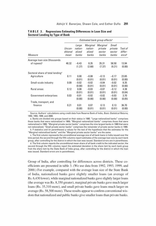
Group of India, after controlling for differences across districts. These co-efficients are presented in table 3. (We use data from 1992, 1993, 1999, and2000.) For example, compared with the average loan size of the State Bankof India, nationalized banks gave slightly smaller loans (an average of Rs. 6,430 lower), while marginal nationalized banks gave slightly larger loans(the average was Rs. 8,350 greater), marginal private banks gave much largerloans (Rs. 35,310 more), and small private banks gave loans much larger onaverage (Rs. 58,500 more). These results appear to confirm conventional wis-dom that nationalized and public banks give smaller loans than private banks.


T A B L E 3 . Regressions Estimating Differences in Loan Size and Sectoral Lending by Type of Bank

Estimated bank group effects a

Large Marginal Marginal Small Uncon- nation- nation- private private Test of ditional alized alized sector sector differ-

Measure mean banks banks banks banks enceb

Average loan size (thousands of rupees)c 48.32 −6.43 8.35 35.31 58.50 13.94

(1.27) (2.68) (7.37) (9.21) (0.00)

Sectoral share of total lendingd

Agriculture 0.11 0.00 −0.08 −0.13 −0.17 23.65(0.01) (0.01) (0.01) (0.01) (0.00)

Small-scale industry 0.09 −0.02 −0.02 −0.04 −0.02 8.35(0.00) (0.01) (0.01) (0.01) (0.00)

Rural areas 0.12 0.08 −0.03 −0.07 −0.12 4.38(0.01) (0.01) (0.01) (0.01) (0.04)

Government enterprises 0.03 -0.01 −0.02 −0.02 −0.03 3.70(0.00) (0.00) (0.00) (0.00) (0.05)

Trade, transport, and finance 0.21 0.01 0.07 0.13 0.13 36.70

(0.00) (0.01) (0.01) (0.01) (0.00)

Source: Authors’ calculations using credit data from Reserve Bank of India, Basic Statistical Returns,1992, 1993, 1999, and 2000.

a. Banks are divided into groups based on their status in 1980. “Large nationalized banks” comprisesthose banks that were nationalized in 1969; “Marginal nationalized banks” comprises those that werenationalized in 1980; “Marginal private sector banks” comprises the nine largest banks in 1980 that werenot nationalized; “Small private sector banks” comprises the remainder of private sector banks in 1980.

b. F-statistics and (in parentheses) p values for the test of the hypothesis that the estimates for the“Marginal nationalized banks” and the “Marginal private sector banks” are the same.

c. The first column represents the unconditional average size of all bank loans in India issued over thetime period; the second through the fifth columns report estimates of the average loan size by each bankgroup, after controlling for the district in which the loan was issued. Standard errors are in parentheses.

d. The first column reports the unconditional mean share of all bank credit to the indicated sector; thesecond through the fifth columns report the estimated deviation in the share lent by each bank groupfrom the share lent by the State Bank of India group, after controlling for the district in which the loanwas issued. Standard errors are in parentheses.


The most informative comparison is between what we called the “marginal”nationalized and the “marginal” private bank, which were similar in size, butwith the former nationalized and the latter not. Many of the differencesbetween the marginal nationalized and the marginal private banks are large:the marginal private banks gave 5 percentage points less credit to agriculturethan the marginal nationalized banks: given that the all-India share of credit toagriculture is 11 percent, this difference is substantial. The results also suggestthat nationalization led to more credit to small-scale industry (an increase of 2 percentage points relative to the private banks; India-wide small-scale indus-try receives 9 percent of total credit), 4 percentage points more credit to ruralareas (compared with a national average of 12 percent), and slightly more togovernment enterprises (0.7 percent more; the India-wide figure is 3 percent.).These increases come at the expense of credit to trade, transport, and finance(nationalized banks gave 6 percent points less, compared with the nationalaverage share of 21 percent). The final column in table 3 gives the results ofan F-test of the hypothesis γMarginal Private = γMarginal Nationalized. The rural and govern-ment lending differences are significant at the 5 percent level, while all othersare significant at the 1 percent level.

Although this finding suggests that private and public banks behave dif-ferently, the values in the table vary not only between marginal private andmarginal nationalized banks, but across other bank groups as well. Thus,from this data alone, we cannot rule out the possibility that the differencein lending behavior is attributable to bank size, rather than ownership.

To obtain an accurate measure of the impact of nationalization, we exam-ine lending behavior at the individual bank level, adopting a full-fledgedregression-discontinuity approach. We first estimate bank effects analogousto the group effects estimated in equation 2, by replacing the bank groupdummy indicators with individual bank dummy indicators, to obtain coeffi-cients β̂1, . . . β̂B. These coefficients tell us to what extent bank b behaves dif-ferently from other banks, after controlling for the characteristics of thedistricts in which each bank operates. We then regress the individual indi-cators β̂b on log deposits of the bank in 1980 (sizeb), an indicator variable(NATb) which takes the value of 1 when the size was larger than the cutoffand the bank therefore nationalized, and an interaction term (NATb * sizeb).This specification thus allows for a break at the nationalization cutoff value,as well as differential slopes for banks below and above the cutoff:

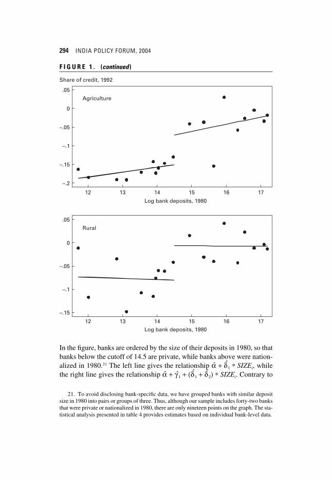
(3) β̂b = α + δ1SIZEi + γ1NATi + δ2(NATb * SIZEb) + εi .

Figure 1 presents the average share each bank provides to small-scaleindustry, “trade, transport, and finance,” agriculture, and in rural areas.




.05

0

–.05

–.1

.3

.2

.1

0

Share of credit, 1992

Small-scale industry

Trade, transport, and finance

12 13 14 15 16 17

12 13 14 15 16 17

Log bank deposits, 1980


F I G U R E 1 . Effects of Nationalization and Trade Credita

Source: Authors calculations, based on data from the Reserve Bank of India.a. Each dot represents the average share of credit of two or three banks provided to the sector indi-

cated in the title. The banks are ordered according to the log size of deposits in 1980, which is graphedalong the x-axis. The left line gives the fitted relationship for the banks that were not nationalized, whilethe line on the right gives the fitted relationship for nationalized banks. The distance between the linesat 14.5 is the implied causal impact of nationalization. The sample includes 42 banks, which were aggre-gated into 19 groups to avoid disclosing any bank-specific information.




.05

0

–.05

–.1

–.15

–.2

.05

0

–.05

–.1

–.15

Share of credit, 1992

Agriculture

Rural

12 13 14 15 16 17

12 13 14 15 16 17


F I G U R E 1 . (continued )

In the figure, banks are ordered by the size of their deposits in 1980, so thatbanks below the cutoff of 14.5 are private, while banks above were nation-alized in 1980.21 The left line gives the relationship α̂ + δ̂1 * SIZEi, whilethe right line gives the relationship α̂ + γ̂ 1 + (δ̂1 + δ̂2) * SIZEi. Contrary to

21. To avoid disclosing bank-specific data, we have grouped banks with similar depositsize in 1980 into pairs or groups of three. Thus, although our sample includes forty-two banksthat were private or nationalized in 1980, there are only nineteen points on the graph. The sta-tistical analysis presented in table 4 provides estimates based on individual bank-level data.


the results obtained by simple comparison of means, there does not appearto be any significant difference in lending to small-scale industry betweenpublic and private banks of similar size. That is, we cannot reject thehypothesis that nationalization had no effect on credit to small-scale indus-try. On the other hand, nationalization appears to have lowered the amountof credit banks provide to trade, transport, and finance.

Nationalization appears to have had a large effect on credit to agricul-ture, as indicated in that panel. There is a relationship between size in 1980and lending to agriculture in 1992: larger banks lend more to agriculture.However, there is a visible break in the relationship at the nationalizationcutoff: banks just above the cutoff lend substantially more to agriculturethan banks just below, even after accounting for the effect of size. The anal-ogous graph for rural credit is also presented.

Table 4 provides estimates of the size of the discontinuity, γ̂1 + δ̂2 * 14.5,estimated on data from 1992 and 2000 separately. For example, for agricul-ture in 1992, the estimated break is .082, with a standard error of .030: thedifference between nationalized and private banks is quite significant, botheconomically and statistically.

The point estimates of the structural break confirm some of the differ-ences described above but suggest that others are merely functions of banksize. In particular, as measured by credit in 1992, nationalization had acausal effect on agricultural credit and rural credit, increasing each byabout 8 percentage points. These numbers are large, given that the set of allbanks lent only 11 percent of credit to agriculture and 12 percent to ruralareas. These results are significant at the 1 percent level. Nationalizationappears to have had no effect on the amount of credit banks lend to small-scale industry, but caused a 9 percentage point decrease in the credit banksissued to trade, transport, and finance. Not surprisingly, we see that nation-alized banks lend more to government-owned enterprises; the 2 percentagepoint difference is particularly large in light of the fact that credit to gov-ernment borrowers represents only 2 percent of bank credit. Public sectorbanks appear to lend at slightly lower interest rates, though the point esti-mate, 70 basis points, is not statistically significant. We also attempted tomeasure whether public sector banks gave more credit to industries that hadbeen identified for support in various five-year plans after 1980, but foundno evidence that these industries were favored.

The differences between the nationalized and private banks seem tohave decreased over time: in the 2000 data, the point estimate on agricul-tural lending drops from 8 to 5 points, on rural lending from 7 to 3 points,and on trade, transport, and finance from −11 to −6 points.



In sum, bank ownership does seem to have had a limited impact on thegovernment’s ability to direct credit to specific sectors. Through the early1990s, the credit environment in India was very tightly regulated. The gov-ernment set interest rates and required both public and private banks toissue 40 percent of credit to the priority sector and to meet specific sub-targets within the priority sector. Nevertheless, banks controlled by thegovernment provided substantially more credit to agriculture, rural areas,and the government, at the expense of credit to trade, transport, and finance.Surprisingly, there was no effect on credit to small-scale industry. Lendingdifferences shrunk over the 1990s and in 2000 to about half what they werein the early 1990s. This might reflect either the increasing dynamism of the


T A B L E 4 . Point Estimates of the Effect of Bank Nationalization on Average Loan Size, Sectoral Lending, and Interest Rates

Estimate of discontinuity a

Measure 1992 2000

Average loan size −24.753 −143.867(10.332) (69.784)

Share of total lendingAgriculture 0.082 0.031

(0.030) (0.021)Rural areas 0.073 0.021

(0.027) (0.023)Small-scale industry 0.009 0.020

(0.017) (0.026)Trade, transport, and finance −0.073 −0.037

(0.040) (0.031)Government enterprisesb 0.020

(0.011)Interest rate (residualc) −0.007 −0.007

(0.008) (0.006)

Sources: Authors’ calculations using data from Reserve Bank of India, Basic Statistical Returns, 1992and 2000.

a. Calculated by estimating the relationship between bank lending behavior and bank size accordingto the following equation:

βi = α + δi SIZEi + γ1NATi + δ2NAT * SIZE + εi,

where SIZEi is the logarithm of deposits of bank i in 1980 and NATi is a dummy variable taking the valueof 1 if the bank was above the threshold for nationalization in 1980, and then evaluating the fitted regres-sion equations for marginal nationalized and marginal private sector banks (as defined in table 3) at thethreshold for nationalization (14.5, in logarithms) and subtracting. Standard errors are in parentheses.

b. Data on lending to government in 2000 were not available.c. Estimated residual from a regression of the interest rate on a range of loan characteristic

variables and district fixed effects. See the notes to the text for a list of all controls.


private sector banks in the liberalized environment of the 1990s or the loos-ening grip of the government on the nationalized banks.

Bank Ownership and Speed of Financial Development

To determine whether public ownership of banks inhibits financial inter-mediation, we again compare banks just above and just below the 1980nationalization cutoff, using data from the Reserve Bank of India, for theperiod 1969 to 2000. We include the six banks above, which were nation-alized, and the nine largest below, which were not.22 Because we have datafrom both before and after the 1980 nationalization, we adopt a difference-in-differences approach. Specifically, we regress the annual change in bankdeposits, credit, and number of bank branches on a dummy for post-nationalization (POSTt = 1 if year ∈ (1980 − 1991)) and a dummy for post-nationalization in a liberalized environment (NINETIESt = 1 if year ∈(1992 − 2000)). We break the post-nationalization analysis up into twoperiods (1980–91 and 1991–2000) because the former period was charac-terized by continued financial repression, while substantial liberalizationmeasures were implemented in the beginning of the 1990s. Public andprivate banks could well behave differently before and after liberalization.Because larger banks may grow at different rates than small banks, weinclude bank fixed effects (βi). We thus regress:

(4)ln (yb,t ⁄yb,t−1) = βi + θ1POSTt + θ2 * NINETIESt +

γ1 (POSTt * NATb) + γ2 (NINETIESt * NATb) + εb,t

The parameters of interest are γ1 and γ2, which capture the differentialbehavior of nationalized banks after the nationalization. Standard errors areadjusted for auto-correlation within each bank.

Table 5 presents the results for growth in credit, deposits, and bankbranches. The results suggest that although the overall rate of growth indeposits and credit slowed substantially during 1980–90 relative to1969–79, there was no differential effect for nationalized and privatebanks. In the nineties, deposit and credit growth slowed further still. In thisliberalized environment, deposits and credit of the nationalized banksslowed more than those of the private banks: deposits grew 7.3 percentmore slowly, while credit grew 8.8 percent more slowly. These results aresignificant at the 10 percent and 5 percent level, respectively.


22. In 1985, the Lakshmi Commercial Bank was merged with Canara Bank, a large pub-lic sector bank, because of financial weakness. In 1993, the New Bank of India (national-ized in 1980) was merged with the Punjab National Bank. Because both the Canara andPunjab National banks were nationalized in 1969, they are not in our sample.


The growth rate in bank branches generally tracked credit and deposits,though the decline after 1980 was more severe. While the growth rates fornationalized banks were slightly lower in both periods, the differences arenot statistically significant.

To answer the question of whether there was a significant differencebetween public and private banks before nationalization, we reestimateequation 4, replacing the bank fixed effects with a nationalizationdummy, and a control function (Kb,80) = π1Kb,80 + π2K2

b,80, which controlsfor the effect of 1980 log deposits of each bank in 1980 (denoted Kb,80).(These results are not reported but are available from the authors.) Thecontrol function allows bank growth to depend on bank size, while thenationalization dummy will pick up any differences between the nation-alized and non-nationalized banks that are not related to size. The esti-mates suggest that credit, deposits, and number of branches grew at thesame speed between 1969 and 1979 for banks that were going to be na-tionalized in 1980 and those that were not. The coefficients on the inter-


T A B L E 5 . Regressions Estimating the Effect of Nationalization on Growth of Deposits, Credit, and Number of Branchesa

Dependent variable

Log real growth of Log growth rate of

No. of No. of rural Independent variable Deposits Credit branches branches

POST −0.085 −0.078 −0.114 −0.181(0.014) (0.015) (0.017) (0.024)

POST * NATIONALIZATION −0.026 −0.012 −0.044 −0.066(0.033) (0.036) (0.033) (0.031)

NINETIES −0.040 −0.027 −0.122 −0.219(0.014) (0.017) (0.018) (0.022)

NINETIES * NATIONALIZATION −0.073 −0.088 −0.053 −0.086(0.039) (0.041) (0.034) (0.028)

R 2 .15 .11 .48 .31No. of observations 440 440 420 434No. of clusters 15 15 14 14

Source: Authors’ calculations from data in Reserve Bank of India, Statistical Tables Relating to Banksin India, 1970–2000, and Directory of Commercial Banks in India, 2000.

a. The sample includes the six banks just above and the nine just below the cutoff for nationalizationin 1980. Branch data were not available for the Lakshmi Commercial Bank, which failed in 1985 and wasmerged with Canara Bank, a large bank nationalized in 1969, which is not in the sample. Underlying datafor deposits and credit are in rupees adjusted for inflation, and data for branches are annual growthrates (all in logarithms). The variable POST takes a value of 1 when the year is from 1980 to 1991 inclu-sive; NINETIES takes the value of 1 when the year is from 1992 to 2000 inclusive; NATIONALIZATIONtakes the value of 1 if the bank was nationalized in 1980. All regressions include bank fixed effects. Stan-dard errors, adjusted for serial correlation, are in parentheses.


action terms (POSTt * NATb) and (NINETIESt * NATb) remain negativeand are virtually unchanged from the specification we present in table 5.Thus, it is only after the 1980 nationalization that banks nationalized in1980 started to grow more slowly. These results provide some evidencethat nationalization hindered the spread of intermediation in the 1990s,but not earlier.

Constraints on Public Sector Lending

Having established that small-scale firms in India are credit constrained,and that, if anything, bank nationalization exacerbated these constraints,we now attempt to determine why public sector banks appear so reluctantto lend. We first look at the rules public sector banks use to allocatecredit, and then examine how the incentives for loan officers affect lend-ing decisions.

Lending Policy

We begin by examining the official rules used by public sector banks toallocate credit. We find the rules surprisingly conservative. Because theoryand praxis often differ, we then examine actual lending decisions and findthat the conservative character of the rules is exacerbated by conservativedeviations from the rules.

OFFICIAL LENDING POLICIES. Although public sector banks in India arenominally independent entities, they are subject to intense regulation by theReserve Bank of India (RBI). Among the rules is one that limits how mucha bank can lend to individual borrowers—the so-called “maximum permis-sible bank finance.” Until 1997, the rule was based on the working capitalgap, defined as the difference between the current assets of the firm and itstotal current liabilities excluding bank finance (other current liabilities).The presumption is that the current assets are illiquid in the very short runand therefore the firm needs to finance them. Trade credit is one source offinance, and what the firm cannot finance in this way constitutes the work-ing capital gap.

Firms were supposed to cover a part of this financing need, correspond-ing to no less than 25 percent of the current assets, from equity. The maxi-mum permissible bank finance under this method was thus:

(5) 0.75 * CURRENT ASSETS − OTHER CURRENT LIABILITIES



The sum of all loans from the banking system was supposed not toexceed this amount.23

This definition of the maximum permissible bank finance applied toloans greater than Rs. 20 million. For loans less than Rs.20 million, bankswere supposed to calculate the limit based on the projected turnover of thefirm. Projected turnover was to be determined by a loan officer in consul-tation with the client. The firm’s financing need was estimated to be 25 per-cent of the projected turnover, and the bank was allowed to finance up to80 percent of what the firm needs, that is, up to 20 percent of the firm’sprojected turnover. The rest, amounting to at least 5 percent of the projectedturnover, has again to be financed by long-term resources available tothe firm.

In the middle of 1997, the RBI set up a committee, headed by P. R.Nayak, to make recommendations regarding the financing of small-scaleindustries. Following the committee’s advice, the RBI decided to give eachbank the flexibility to evolve its own lending policy, under the conditionthat it be made explicit. Moreover, they adopted the recommendation thatthe turnover rule be used to calculate the lending limit for all loans less thanRs. 40 million.

Given the freedom to choose the rule, different banks went for slightlydifferent strategies. The bank we studied adopted a policy that was, ineffect, a mix between the now recommended turnover-based rule and theolder rule based on the firm’s asset position. First the limit on turnover basiswas calculated as:

(6)min(0.20 * Projected turnover, 0.25 * Projected turnover− Available margin).

The available margin here is the financing available to the firm from long-term sources (such as equity) and is calculated as CURRENTASSETS − CURRENT LIABILITIES from the current balance sheet. Inother words, the presumption is that the firm has somehow managed tofinance this gap in the current period and therefore should be able to doso in the future. Therefore the bank needs to finance only the remainingamount. Note that if the firm had previously managed to get the bank tofollow the turnover-based rule exactly, its available margin would beprecisely 5 percent of turnover and the two amounts in equation 6 wouldbe equal.


23. Thus, a particular bank had to deduct from this amount the credit limits offered byother banks. Following this rule implies that the current ratio will be more than 1.33, andthe rule is often formulated as the requirement that the current ratio exceeds 1.33.


The rule did not stop here. For all loans less than Rs. 40 million (as allloans in our sample are), the loan officer was supposed to use both equa-tion 6 and the older rule represented by equation 5. The largest permissiblelimit on the loan was the maximum of these two numbers.

Two comments about the nature of this rule are in order. First, thisturnover-based approach to working capital finance is relatively standardeven in the United States. However, the view in the United States is thatworking capital finance is essentially financing inventories and is thereforebacked by the value of the inventories. In India, the inventories do not seemto provide adequate security, as evidenced by the high rates of default. Insuch cases it may be much more important to pay attention to profitability,because profitable companies are less likely to default. Second, in the UnitedStates the role of finding promising firms and promoting them is carried outlargely by venture capitalists. In India the venture capital industry is stillnascent and is not yet able to play the role that we expect of its U.S. equiv-alent. Therefore banks may have to be more proactive in promoting promis-ing firms. Following a rule that puts no weight on profits may not be the wayto favor the most promising firms: although the projected turnover calcula-tion does favor faster-growing firms, the loan officer is not allowed to pro-ject a growth rate greater than 15 percent. This may be enough to meet theneeds of a mature firm, but a small firm that is growing fast clearly needsmuch more than 15 percent. It is important that the rules encourage the loanofficers to lend more to companies on the basis of promise.

ACTUAL LENDING POLICY. The lending policy statements give us theoutside limits on what the banks can lend. Nothing in the policies stopsthem from lending less, though official documents always enjoin bankersto lend as much as possible.24 It is also possible, given that it is not clearhow these rules are enforced, that the banks sometimes exceed the limits—it is, for example, often alleged that loan officers in public sector banks giveout irresponsibly large loans to their friends and business associates. It isnot even clear how one would necessarily know that a banker had lent toomuch given that he is given the task of estimating expected turnover. In thissubsection, based on work by Banerjee and Duflo, we therefore look at theactual practice of lending in our sample of loans.25


24. For example, a document prepared for the board meeting of the bank we studiedreads “The busy season credit policy announced by the Reserve Bank of India stresses onincrease in credit off-take by imparting further liquidity into the system and by rationaliz-ing some of the existing guidelines. Banks have, therefore, to pay special attention to thisaspect in the coming months and locate all potential/viable avenues so as to accelerate thepath of credit expansion.”



Data: Our data source is the same used in previous work by Banerjeeand Duflo (and described in connection with equation 1).26 Because wehave data on current assets and other current liabilities, it is simple to cal-culate the limit according to the traditional, working capital gap–basedmethod of lending (henceforth LWC). We can also calculate the limit onturnover basis (henceforth LTB). The maximum of LTB and LWC is,according to the rules, the real limit on how much the banker can lend tothe firm.

Results: In table 6, we compare the actual limit granted with LTB,LWC. In 78 percent of the cases, the limit granted is smaller than theamount permitted. Most strikingly, in 64 percent of the cases for which weknow the amount granted in the previous period, the amount granted isexactly equal to that granted in the previous period (it is smaller 4 percentof the time and goes up only in 31 percent of the cases). Given that thatinflation rate was 5 percent or higher, the real amount of the loans thereforedecreases between two adjacent years in a majority of the cases. To makematters worse, in 73 percent of these cases the firm’s sales had increased,implying, one presumes, a greater demand for working capital. Further, thisis the case even though according to the bank’s own rules, the limit couldhave gone up in 64 percent of the cases (note that getting a higher limit issimply an option and does not cost the firm anything unless it uses themoney). Finally, this tendency seems to become more pronounced over



T A B L E 6 . Actual Credit Limits Granted to Firms Compared with Permissible Limits

Limit actually Limit actually Limit actually Limit officially granted versus granted versus granted versus permitted versus

limit on turnover limit officially previous limit limit previously basis permitted a granted b permitted c

No. of Percent No. of Percent No. of Percent No. of Percent firms of total firms of total firms of total firms of total

Smaller 255 62 542 78 22 4 153 35Same 81 20 9 1 322 64 6 1Larger 74 18 142 20 158 31 281 64

Source: Authors’ calculations from account-level data from one large public sector bank in Indiaduring 1997–99.

a. Maximum officially permitted credit limit is the larger of the limit calculated by the turnover methodor that calculated by the working capital gap method.

b. “Previous limit granted” is the amount offered to the same firm the year before. c. “Limit previously permitted” is the value of the official limit for the firm in the previous year.


time: in 1997, the limit was equal to the previous granted limit 53 percentof the time. In 1999, it remained unchanged in 70 percent of the cases.

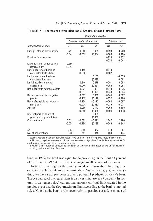
In table 7, we regress the limit granted on information that might beexpected to play a role in its determination. Not surprisingly, given every-thing we have said, past loan is a very powerful predictor of today’s loan.The R-squared of the regressions is also very high (over 95 percent). In col-umn 1, we regress (log) current loan amount on (log) limit granted in theprevious year and the (log) maximum limit according to the bank’s internalrules. Note that the bank’s rule never refers to past loan as a determinant of


T A B L E 7 . Regressions Explaining Actual Credit Limits and Interest Ratesa

Dependent variable

Actual credit limit granted Interest rate

Independent variable (1) (2) (3) (4) (5)

Limit granted in previous year 0.757 0.540 0.455 −−0.198 −−0.260(0.04) (0.059) (0.084) (0.108) (0.124)

Previous interest rate 0.823 0.832(0.038) (0.041)

Maximum limit under bank’s 0.256internal ruleb (0.042)

Limit on turnover basis as 0.145 −−0.019calculated by the bank (0.036) (0.102)

Limit on turnover basis as 0.102 −−0.025calculated by authorsc (0.025) (0.09)

Limit based on working 0.240 0.279 0.091 0.083capital gap (0.046) (0.061) (0.083) (0.084)

Ratio of profits to firm’s assets 0.021 −−0.001 −−0.048 −−0.036(0.017) (0.021) (0.043) (0.044)

Dummy variable for negative −−0.037 0.053 −−0.045 −−0.037profits (0.115) (0.129) (0.272) (0.266)

Ratio of tangible net worth to −−0.104 −−0.112 −−0.064 −−0.087firm’s debt (0.029) (0.032) (0.076) (0.07)

Assets 0.080 0.143 0.063 0.168(0.056) (0.065) (0.104) (0.118)

Interest paid as share of 0.005year-before granted limit (0.037)

Constant term 0.011 −−0.009 −−0.021 2.547 2.180(0.079) (0.154) (0.195) (0.749) (0.843)

R 2 .952 .955 .962 .878 .881No. of observations 298 241 145 198 194

Source: Authors’ calculations from account-level data from one large public sector bank in India.a. All data except interest rates and dummy variables are in logarithms. Standard errors, corrected for

clustering at the account level, are in parentheses.b. Higher of limit based on turnover as calculated by the bank or limit based on working capital gap.c. Using bank’s projection of turnover.


the loan amount to be given out. Yet the coefficient of past loan is 0.757,with a t statistic of 18 (a 1 percent increase in past loan is associated with a0.756 percent increase in current loan, after controlling for the official rule).The maximum limit is also a significant determinant of loan amount, witha coefficient of 0.256. The standard deviation of these two variables is veryclose (1.50 and 1.499, respectively). These coefficients thus mean that aone standard deviation increase in the log of the previous granted limitincreases the log of the granted limit by three times as much as a one stan-dard deviation increase in the log of the maximum limit as calculated bythe bank.

In column 2, we “unpack” the official limit: we include separately thebank’s limit on turnover basis (LTB) and the limit based on the traditionalmethod (LWC) and now include the logarithm of profits. As in the previ-ous regression, past loan is the most powerful predictor of current loan.Both limits enter the regression. Neither the log of profit nor the dummy fornegative profit enter the regression, as might have been expected given thenature of the rules.

In column 3 we include in addition a measure of the utilization by theclient of the limit granted to him in the previous year: the ratio of interestearned by the bank to the account limit. This is clearly of direct interest tothe bank, because it loses money when funds are committed, but not used.This information is routinely collected on each client. Yet this variable isuncorrelated with granted limit. We tried other measures of utilization ofthe limit (turnover on the account divided by granted limit, and maximumdebt divided by granted limit), and none of these measures is significant.

In columns 4 and 5 we investigate the determinants of interest rates. Pastinterest rates seem to be the only significant determinant of today’s interestrates. Past loans, LTB, and LWC do not enter the regression.

In sum, the actual policy followed by the bank seems to be characterizedby systematic deviation from what the rules permit in the direction of iner-tia. To the extent that limits do change, what seems to matter is the size ofthe firm, as measured by its turnover and outlay, and not profitability or theutilization of the limit by the client.

It could be argued that inertia is rational: the past loan amount picks upall the information that the loan officer has accumulated about the firm thatwe do not observe. But this explanation does not fit well with the fact thatthe loan amount remains exactly the same—the past may be important, but,as noted, the firm’s needs are changing, if only because of inflation.

There is also a simple test of this view. The weight on past loans repre-sents the bank’s experience with the firm: the fact that the weight is so high



presumably reflects the fact that the past is very informative, suggesting astable environment. But a stable environment necessarily implies that thebank knows a lot more about its old clients than it does about its newestclients. Therefore we should see the weight going up sharply with the ageof the firm. Yet when we run the regressions predicting the loan amountseparately for firms that have been the client of the bank for 5 years or moreand for those who have been clients for less than 5 years, we find that banksdo not put less weight on the past loans for recent clients than for oldclients. If anything, when we include today’s sales in the regression thebank seems to put more weight on past loans for recent clients than for oldclients.27 If there is a good reason for the inertia, it has to be somethingmuch more complicated.

It is also conceivable that it is rational to ignore profit information inlending if the projected turnover calculated by the bank and included in thecalculation of LTB already takes into account any useful informationcontained in the profits. To examine this, we looked at whether currentprofitability has any role in predicting future profitability, delay in repay-ment, and default, once we control for the variables that seem to determinethe level of lending—past loans, LTB, LWC. As reported in Banerjee andDuflo, current profit is a good predictor of future profit, and the variablesthat the bank uses are not: the only good predictor of future negative profitis current negative profit.28 Negative profits, in turn, predict default, whilepast loans, LTB, and LWC do not.29

Conclusion: This subsection suggests an extremely simple prima facieexplanation of why many firms in India seem to be starved of credit. Thenationalized banks, or at least the one we study (but again, this is one of thebest public banks), seem to be remarkably reluctant to make fresh lendingdecisions: in two-thirds of the cases, there is no change in the nominal loanamount from year to year. While the rules for lending are indeed fairlyrigid, this inertia seems to go substantially beyond what the rules dictate.Moreover, the deviations from the rules do not seem to reflect informedjudgments, but rather a desire to do as little as possible.

Moreover, when banks take a decision to make a fresh loan, the benefi-ciaries tend to be firms whose turnover is growing regardless of profitabil-ity. This indifference to profitability is entirely consistent with the rules thatbankers work with: none of the many calculations that bankers are sup-posed to do before they decide on the loan amount pays even lip service to


27. See Banerjee and Duflo (2001, table 5).28. Banerjee and Duflo (2001).29. There is some question about whether we have the right measure of default.


the need to identify the most profitable borrowers. Yet current profits do amuch better job of predicting future losses and therefore future defaults,than do the variables that seem to influence the lending decision. In otherwords, it seems plausible that a banker who made better use of profit infor-mation would do a better job at avoiding defaults. Moreover, he or shemight do a better job of identifying the firms where the marginal product ofcapital is the highest. Lending based on turnover, by contrast, may skew thelending process toward firms that have been able to finance growth out ofinternal resources and therefore do not need the capital nearly as much.

What Causes Under-Lending?

Given that the rules for lending are quite rigid and largely indifferent toprofitability, it is perhaps not surprising that there are opportunities forprofitable investment that have not yet been exploited. What is surprisingis that to the extent that there are deviations from the rules, they tend to bein the direction of lending less.

One plausible explanation is that the loan officers in these banks have noparticular incentive to lend. As government employees on a more or lessfixed salary and promotion schedule, their rewards are at best weakly tiedto their success in making imaginative lending decisions. And failed loans,as discussed below, can lead to investigations by the Central VigilanceCommission, the body entrusted to investigate fraud in the public sector.Loan officers therefore have much to lose and little to gain from beingaggressive in lending. Not taking any new decisions may dominate anyother course of action, especially if there are attractive alternatives to lend-ing, such as putting money in government bonds.

The next sub-section examines how the fear of prosecution discourageslending. The following sub-section asks whether the reluctance to lend isexacerbated when the rewards from putting money in government bondsbecome relatively more attractive.

INERTIA AND THE FEAR OF PROSECUTION. Because public sector banksare owned by the government, their employees are treated by law as publicservants subject to government anti-corruption legislation. Bankers believethat it is easy to be charged with corruption and that the law states that anygovernment functionary who takes a decision that results in direct financialgain to a third party is prima facie guilty of corruption and must prove heror his innocence.

The executive director of a large public sector bank was quoted saying“Fear of prosecution for corruption hangs over every loan officer’s head



like the sword of Damocles.” The Economic Times of India has attributedslowdowns in lending directly to vigilance activity.30 A working groupon banking policy set up by the Reserve Bank of India, and chaired byM. S. Verma, noted:

The [working group] observed that it has received representations from the man-agements and the unions of the banks complaining about the diffidence in tak-ing credit decisions with which the banks are beset at present. This is due toinvestigations by outside agencies on the accountability of staff in respect ofsome of the NPA. The group also noticed a marked reluctance at various levelsto take any credit decision.31

In response to criticism from bankers, economists, and others, the CentralVigilance Commission (CVC), the body entrusted to investigate potentialcases of fraud in the public sector, introduced in 1999 a special chapter of thevigilance manual on vigilance in public sector banks. Although the newchapter was meant to reassure bankers, it may not have been entirely suc-cessful. The manual reads, for example, that although “every loss caused tothe organization, either in pecuniary or non-pecuniary terms, need not neces-sarily become the subject matter of a vigilance inquiry . . . once a vigilanceangle is evident, it becomes necessary to determine through an impartialinvestigation as to what went wrong and who is accountable for the same.”32

Interviews with public sector bankers revealed widespread concern: thelegal proceedings surrounding charges of corruption can drag on for years,leaving individuals charged with corruption in an uncertain state. Even ifan individual is exonerated, he or she may have been relieved of duties,transferred, or passed over for promotion during the investigation. In the-ory, as well as practice, even one loan gone bad may be sufficient to startvigilance proceedings. The possible penalties stand in stark contrast torewards. While banks are constantly urged by the Reserve Bank of India tolend as much as possible, there are neither explicit incentives for makinggood loans nor ways to penalize officers who make conservative decisions.In effect, bankers are accountable to more than one authority—the loanofficer’s boss is one, central vigilance may be another, and the press yetanother. In such circumstances, it may be difficult to provide effectiveincentives.33 If so, loan officers would prefer not to take new decisions.


30. “CVC Issues New Norms to Check Bank Frauds,” Hindustan Times (1998), amongothers.

31. Quoted in Tannan (2001, p. 1579).32. Government of India (2001, p. 5).33. Dixit (1996) describes how the presence of multiple principles in bureaucracies may

lead to inaction.


Simply renewing the loan without changing the amount is one easy way toavoid responsibility, especially if the original decision was someone else’s(loan officers are frequently transferred). And when bankers do take a deci-sion, making sure not to deviate enormously from the precedent is a way ofcovering themselves against charges of wrongdoing or worse.

Not surprisingly, the Central Vigilance Commission disputes the claimthat there is a “fear psychosis” and to bolster its position released in 2000 a“critical analysis” of vigilance activity in public sector banks in 1999. Theanalysis reveals that in 1999 the commission received 1,916 references,72 percent of which were credit-related, recommending punishment in themajority of cases. Their report states that “out of every 100 cases comingbefore it, the Commission would advise major penalty proceedings in28 cases, minor penalty proceedings in 32 cases, and administrativewarning/exoneration in 40 cases.”34 The author of the report, a CVC official,argued that this level of activity should not be enough to cause “fear psy-choses”: “These figures reveal that a person is not damned the moment hiscase is referred to the Commission. . . . These statistics appear to indicate avery fair and objective approach on the part of the Commission to the casesthat were referred to it.”35

The rest of this subsection, based on work by Cole, assesses the evidencefor the fear psychosis.36 The idea is simple: do bankers who are “close to”bankers who have been subject to CVC action slow down lending in theaftermath of that particular action?

Data: Monthly credit data, by bank, were provided by the RBI. Data onfrauds are naturally difficult to come by. It is also the policy of the govern-ment of India to keep the data on vigilance activity confidential: althoughsome statistics are published, they are too aggregated to be useful foreconometric analysis. However, in 1998, in an effort to increase the penaltyfor fraud through stigma, the government authorized the CVC to publishthe name, position, employing bank, and punishment of individual officersof government agencies charged with major frauds. This list consists ofeighty-seven officials in public sector banks between 1992 and 2001.Although the nature of the fraud with which they are charged is not known,we do know that approximately 72 percent of frauds relate to illegal exten-sion of credit, with the balance classified as kite-flying or “other.”37

Because our hypothesis is that vigilance decreases lending activity, the


34. Government of India (2000, p. 9).35. Government of India (2000, p.10).36. Cole (2002).37. Government of India (2000).


inclusion of spurious non-credit-related vigilance activity should bias coef-ficients toward zero.

Empirical Analysis: The first approach is to use bank-level monthlylending data to estimate the effect of vigilance activity on lending, using thefollowing equation,

(7) yit = αi + βt + ∑w

k=0γkDi,t−k + εit

where yit is log credit extended by bank i in month t, αi is a bank fixed effect,βt is a month fixed effect, and Di,t−k is an indicator variable for whether vig-ilance activity was reported by the CVC for bank i in month t − k. Standarderrors reported are adjusted for serial correlation and heteroskedasticity.The idea is to compare the bank affected by the vigilance activity with otherpublic sector banks before and after the vigilance event. Which event win-dow to use is not immediately clear: the appropriate start date would mostlikely be the month when it became known that vigilance proceedings wereunder way or perhaps the date bankers learned of the judgment. The datapublished by the CVC give only the date when the CVC provided adviceon the case and the date on which action was taken. It is not clear how longit should take before an effect appears or how long one would expect thiseffect to last. We therefore let the data decide, by estimating models thatallow effects ranging from one month to four years.

Table 8 presents estimation results from several similar specifications.Columns 1, 2, and 3 provide estimates for windows of one, twelve, andforty-eight months. There appears to be a clear effect of vigilance activityon lending decisions. Vigilance activity in a specific bank reduces creditsupplied by all the branches of that bank by about 3-5 percent. This effectis estimated precisely and is significantly different from zero at the 5 per-cent level for contemporaneous effect (column 1) and at the 1 percent levelfor the joint parameters of zero to twenty-four months in columns 2 and 3.The effect is quite persistent, appearing in the data at its original level forup to eighteen months following the vigilance activity, finally becomingstatistically indistinguishable from zero two years after the CVC decisionor judgment.

This economic effect seems to be sizable for plausible values of the elas-ticity of gross domestic product with respect to money supply elasticity.For example, if the overall coefficient of 0.03 were accurate for a bank suchas the State Bank of India, which provides approximately a quarter of thecredit in the economy, decisions on whether to pursue vigilance cases couldhave measurable macroeconomic effects.



Columns 4 and 5 of table 8 present the same specification as in equa-tion 7, but this time with dummies indicating whether a given bank-monthis exactly n months before CVC vigilance activity.

Table 8 clearly indicates that banks reduced lending before the announcedvigilance action, as well as after it. This is not surprising, as the formal vig-ilance activity usually follows a lengthy investigation. The CVC vigilancemanual, introduced in 1999 to streamline the process of investigations, out-lines a procedure that lists no binding time constraints, but suggests the


T A B L E 8 . Regressions Estimating Effect of Indicators of Vigilance Activityon Bank Credita

Regressions measuring

Months beforeRegressions measuring effect effect of future vigilance

or after of previous vigilance activity activity

vigilance activity b (1) (2) (3) (4) (5)

Zero −0.055 −0.040 −0.037 −0.042 −0.037(0.027) (0.019) (0.019) (0.020) (0.020)

Three −0.039 −0.032 −0.035 −0.031(0.018) (0.016) (0.016) (0.016)

Six −0.031 −0.023 −0.029 −0.027(0.016) (0.014) (0.015) (0.014)

Twelve −0.036 −0.018 −0.018 −0.015(0.016) (0.012) (0.014) (0.010)

Eighteen −0.028 −0.006(0.013) (0.010)

Twenty-four −0.012 −0.001(0.013) (0.011)

Thirty-six −0.014 0.009(0.015) (0.008)

Forty-eight −0.022 0.022(0.028) (0.015)

R 2 .98 .98 .98 .98 .98No. of observations 2,997 2,997 2,997 2,997 2,997

Source: Authors’ calculations using data from the Reserve Bank of India and the Central VigilanceCommission of India.

a. The dependent variable in all regressions is the logarithm of credit extended by an individual bankin a given month. Data are for twenty-seven public sector banks over 111 months. Standard errors,corrected for heteroskedasticity and serial correlation, are in parentheses.

b. Vigilance activity is defined as the CVC bringing charges against or punishing an officer of a bank.The independent variable of interest is a dummy variable that takes the value of 1 when vigilance activ-ity occurred with respect to a particular bank the indicated number of months before (columns 1–3) orafter (columns 4–5) the current month. The regression in column (1) includes a month dummy for themonth contemporaneous with the vigilance activity only. In columns (2) and (4), month dummies areincluded for each of the twelve months before or after the vigilance activity, respectively, and in columns(3) and (5), month dummies are included for each of the forty-eight months before or after (only selectedmonth coefficients are reported). All regressions also include bank and year fixed effects.


entire process be completed within twenty months. Reassuringly, there isno discernable effect for vigilance activity farther out than one year ahead.

Conclusion: Evidence suggests that the fear of being investigated is re-ducing lending significantly: banks where someone is being investigatedslow down lending relative to their own mean level of lending. This find-ing leaves open the question of whether this reaction is desirable; it is, afterall, possible that the loans that are cut are those unlikely to be repaid. Butthe finding also raises the possibility that honest lenders are being discour-aged by excessively stringent regulations.

LENDING TO THE GOVERNMENT AND THE EASY LIFE. Lending to thegovernment is the natural alternative to lending to firms and offers the loanofficers a secure vehicle for their money, with none of the legwork andheadaches associated with lending to firms. The ideal way to measure howimportant high interest rates on government bonds might be in explainingunder-lending would be to estimate the elasticity of bank lending to the pri-vate sector with respect to the interest rate on government securities or thespread between the interest rate on private loans and that on governmentsecurities. The problem is that the part of the variation that comes fromchanges in the rate paid by the government is the same for all banks andtherefore is indistinguishable from any other time-varying effect on lend-ing. The part that comes from the rates charged by the banks does vary bybank but cannot possibly be independent of demand conditions in the bankand other unobserved time-varying bank-specific factors. One cannottherefore hope to estimate the true elasticity of lending by regressing loanson the spread.

Our strategy is to focus on a more limited question: are banks moreresponsive to the central bank interest rates in slow-growing environments?We start by identifying the banks that are particularly likely to be heavilyinvested in the “easy life.” These are banks that, for historical reasons, havemost of their branches in the states that are currently growing more slowlythan the rest. Our hypothesis is that these banks have a particularly strongreason to invest heavily in government securities, because in a slow-growing environment it is harder to identify really promising clients. Theyalso probably have more “marginal” loans that they are willing to cut andreduce (or not increase) when the interest rate paid to government bonds in-creases. These banks therefore should be particularly responsive to changesin the interest rate paid by the government.

Data: The outcome we focus on is the ln(credit/deposit ratio) at the endof March of each year for twenty-five public sector and twenty private sec-tor banks. Two minor public sector banks were excluded because of lack of



data, and the new private sector banks were excluded for reasons of com-parability. The data are from the Reserve Bank of India.

Data on the net state domestic product are from the Central StatisticalOffice. For our measure of interest rate spread, we subtract from the StateBank of India prime lending rate, the rate given as the weighted average ofcentral government securities. Both interest rate measures are from theRBI, as is the price index used to deflate them.38

Specification: Two measures of growth are used. To measure the stategrowth rate (growthit = ln(SDPit) − ln(SDPi,t−1)), we use a moving aver-age of the real growth rates of the previous three years (e.g., avgrowthit =∑t−1

t−3(growthit). Bank environment growth is a weighted average of thegrowth rates in the states in which a bank operates:

bkgrowthbit = ∑i∈states

ωbi avgrowthbit

where the weights ωbi are the percentage of bank branches bank b had in

state i in 1980: . Data on branch locations are from the of

Directory Commercial Bank Offices in India.39

Results: We test this hypothesis with two pairs of linear regressions. First,we consider using the location of a bank’s headquarters as an indicator of thegrowth environment in which a bank operates. Because the regulatoryenvironment in India changed significantly beginning during 1991–92, weestimate our equations for the entire time period, 1985–2000, as well as the“post-reform period” of 1992–2000.

The results are reported in table 9. Columns 1 and 2 report the resultsusing the growth environment of the state in which a bank is headquartered,


38. Data are from the 2001 edition of RBI, “Handbook of Statistics on the Indian Econ-omy.” We use the CPI-UNME, for Urban Non-Manual Employees.

39. Branch data are from Reserve Bank of India (2001). We have NSDP for all of thestates in which bank headquarters are located. However, in constructing the index, NSDPfor the following were not available: Jharkhand, Uttaranchal, Chandigrah, Dadra and NagarHaveli, Chattisgarh, and Lakhsadeep. Rather than drop any bank that had a branch in one ofthese states, the ωbi weights are constructed using only the set of branches for which GSPdata are available. A second problem is that the growth data are not available for a few statesfor 1998 and 1999 (Nagaland, Sikkim, Andaman and Nicobar) or 1999 (Goa, Jammu &Kashmir). The two most logical ways of constructing indexes in the absence of these data,namely (i) not using those states when constructing state weights, and thus not using thegrowth information during 1985–97, and (ii) using one set of weights ωbi

1 during 1985–97,which includes these states, and a second set ω bi

2 , which excludes these states in 1998 and1999, produce essentially identical results. We choose the latter, because we feel Jammuand Kashmir and Goa warrant inclusion throughout 1985–98.

ωbi =∑s∈states Nbs

Nbi


with the first column representing the results for the entire period and thesecond, results for the post-reform era. Specifically, we estimate

(8)ln (CDbit) = α + β * avgrowthbit + γ + (Spreadt * avgrowthbit) * ISpreadt>0

+ γ − (Spreadt * avgrowthbit) * ISpreadt<0 + θi + δt + εbit ,

where ISpreadt>0 (resp. ISpreadt<0) are indicator variables for whether the spreadis positive (resp. negative), θi is a state fixed effect, and δt is a year fixedeffect. Avgrowthbit is the smoothed growth rate for the state where theheadquarters of bank b are located. Standard errors are adjusted for serialcorrelation.

The regression controls for state and year fixed effects. While we seethat the C/D is higher in states with more favorable growth rates, we aremost interested in the coefficients γ − and γ +, which measure how banks indifferent growth environments differentially react to changes in the spreadbetween the commercial lending rate and the rate on government securities.


T A B L E 9 . Regressions Explaining Bank Credit with Spreads on Creditand Economic Growth by Statea

Growth measure b

Growth in net state Weighted average of domestic product in state growth rates in states

where bank is headquartered where bank operatesc

Independent variable 1992–2000 1985–2000 1992–2000 1985–2000

Growth rate 1.412 1.538 2.195 2.634(0.624) (1.209) (0.970) (1.165)

Growth rate * (spread > 0) −0.175 −0.137 −0.257 −0.219(γ +) (0.110) (0.119) (0.104) (0.103)Growth rate * (spread < 0) 0.480 0.592 −0.079 0.473(γ −) (0.521) (0.405) (0.791) (0.562)

State fixed effects? Yes Yes No NoBank fixed effects? No No Yes Yes

R 2 .46 .43 .71 .63No. of observations 415 730 402 710

Source: Authors’ regressions using data from the Reserve Bank of India.a. The dependent variable in all regressions is the logarithm of the ratio of credit extended to deposits.

Data are annual data for twenty-five public sector and twenty private sector banks. Standard errors,corrected for heteroskedasticity and serial correlation, are in parentheses. All regressions includeyear fixed effects.

b. In all regressions growth is measured as a moving average of real growth rates over the previousthree years.

c. Fewer observations are available for these regressions because data on branch locations wereunavailable for one bank.


Because a negative spread occurs only twice, and in a quite particular situ-ation (in a perfectly flexible market, banks facing a negative spread shouldeliminate all credit from their portfolios), we allow a separate coefficient on(Spreadt * avgrowthbit) when the spread is negative.

The negative and marginally statistically significant coefficient on γ +

suggests that banks in high-growth environments substitute toward gov-ernment securities (away from loans) less when the spread falls. We inter-pret this to mean that banks in low-growth states are more sensitive togovernment interest rates: because they face fewer attractive projects tofinance, they are more likely to park money in government securitieswhen government securities become more attractive. However, becausethe number of states where a bank is headquartered is relatively low, we have relatively low power once we account for serial correlation at thestate level.

To achieve more precise estimates, we estimate the same equation, ex-cept that instead of measuring growth only in the states where commercialbanks are headquartered, we use the synthetic index described above,which takes into account all the states where the bank is active. Columns 3and 4 present results from:

(9)ln (CDbit) = α + β * bkgrowthbit + γ + (Spreadt * bkgrowthbit) * ISpreadt>0

+ γ − (Spreadt * bkgrowthbit) * ISpreadt<0 + θi + ψb + δt + εbit ,

where bkgrowthbit is the growth index and ψb is a bank fixed effect. Col-umn 3 represents the entire sample, while column 4 represents the post-reform period. The results in columns 3 and 4 are similar in sign tocolumns 1 and 2, and this time we may say with some confidence thatthey are statistically significant.

Conclusion: The evidence seems consistent with the view that banks areespecially inclined toward the easy life in states where lending is hard. Thissuggests that the opportunity for lending to the government tends to hurt thefirms that are relatively marginal from the point of view of the banks, suchas firms in slow-growing states and smaller and less established firms.

Some Final Issues: Rural Branches, NPAs and Bailouts

We conclude our study by examining two final arguments given in favor ofpublic ownership of banks: that public banks are more willing to expandinto rural areas and that public banks are less likely to fail and therefore costthe government (or public) less than private banks.



Branch Expansion in Rural Areas

As mentioned in the introduction, in 1977 the government passed a regula-tion requiring both public and private banks to open four branches inunbanked locations for every branch they opened in banked locations. Thisregulation was repealed in 1990, though the Reserve Bank of India stillmaintained some authority of bank branch openings.

Robin Burgess and Rohini Pande have studied the impact of this regula-tion over the period 1977–90.40 They find that a 1 percent increase in thenumber of rural banked locations, per capita, resulted in a 0.42 percentdecline in poverty, and a 0.34 percent increase in total output.

Cole uses the empirical strategy described in the section on “Bank Own-ership and Sectoral Allocation of Credit” to study the impact of banknationalization on rural bank growth.41 He shows that between 1980 and2000 the growth rate of rural branches fell substantially, on the order of20 percent. The nationalized banks in our sample fell even more sharply,with rural branch growth rates 6.6 percent and 8.6 percent slower than theirprivate counterparts in the 1980s and 1990s. These results are reported incolumn 4 of table 5.

In summary, the regulation requiring the opening of rural banks maywell have been beneficial, but, if anything, nationalization made banksslightly less responsive to the regulation.

Non-Performing Assets and Bailouts

Mounting nonperforming assets and resulting questions about the ability ofthe banks with high levels of NPA to honor their liabilities to their deposi-tors have been important concerns in the 1990s.

Recent RBI figures suggest that public sector banks have substantiallyhigher levels of nonperforming assets than do private banks. For example,for the year ending in March 2003, gross NPAs represented 4.6 percent ofpublic sector banks’ total assets, as against 4.3 percent of those of old pri-vate sector banks and 3.7 percent of those of new private sector banks. It isnot clear, however, how well these numbers represent the true situation inthese banks. There is some skepticism about the accuracy of reported NPAnumbers: banks may engage in creative accounting or “evergreening,” andthe current classification norms mapping loan repayment delay to NPA donot yet meet international norms.


40. Burgess and Pande (2003).41. Cole (2004).


An informative check, conducted by Petia Topalova, is to use datafrom corporate balance sheets to estimate the ability of firms to repay theirloans.42 Firms whose income (defined as earnings before interest, taxes,depreciation, and amortization) is less than their reported interest expenseare either defaulting, are very close to default, or would be defaulting iftheir loans were not “evergreened.” This share of “potential NPAs” hasincreased significantly in the past five years, while banks’ reported level ofNPAs has stayed fairly constant. Topalova also finds that banks areexposed to substantial interest rate risk: a 200 basis point increase in therate of interest could result in a 4 percentage point increase in the share ofNPAs in the banking system.

These high levels of NPAs raise obvious concerns about the stability ofindividual banks. But the government’s policy so far has been to allay theseconcerns by simply taking over the uncovered liabilities of the failingbanks, whether nationalized or private. Therefore we will measure the costof the NPAs in terms of resources that have gone into bailing out thesebanks.

We are not aware of a systematic accounting of all bank failures in Indiasince 1969. To calculate the cost of bank failures, we use data collectedfrom annual issues of the RBI’s Statistical Tables Relating to Banks inIndia, starting in 1969. Although the data are not comprehensive, we areoptimistic that they can provide at least the correct order of magnitude.43

In 1969, we have deposits data for forty-five private sector banks.Between 1969 and 2000, we are able to identify twenty-one cases of bankfailure, which resulted either in a bank’s liquidation or its merger with apublic sector bank. (An additional twenty banks were nationalized: four-teen in 1969, and six in 1980. We do not count these twenty nationaliza-tions as failures.) The value of the deposits at the time the bank failed canbe taken as an upper bound of the cost of a bank failure. Thus, we calculatethe value (in Rs. 2000) of the deposits of these twenty-one banks.44 Thelargest single failure was Laxhmi Commercial Bank, which merged withCanara Bank in 1985 and represents 18.5 percent of the share of real deposits


42. Topalova (2004).43. For example, the data may not correctly account for the possibility that banks

change their names or merge while healthy. We identify the failure of private sector banksby their disappearance from our data: in many cases, these failures can be confirmed by sec-ondary sources, but it is possible (even likely) that we have missed some failures, or evalu-ated as bank failures some events that were not failures. We would welcome a more carefulstudy of this issue.

44. For all price adjustments in this section, we use the consumer price index from theInternational Financial Statistics database of the International Monetary Fund.


of failed banks. The total value of deposits for banks that failed between1969 and 2000 is approximately Rs. 45 billion, a substantial sum.45

The total cost of recapitalization is also unknown. We conduct a back-of-the-envelope exercise, using figures from the 1999–2000 issue of the RBI’sReport on Trends and Progress of Banking in India.46 These figures give thecapital contribution of the central government to nationalized banks, as wellas the amount of capital written down by the central government. Whileinterpretation of the write-off is straightforward, the recapitalization fundingrequires a little work. Banks earned money from the recapitalization bonds.The recapitalization subscription will, at least in theory, be returned to thegovernment (several public sector banks have already returned capital): thus,the true cost of recapitalization is best measured by the interest income for-gone by the government. The 2000–01 Report on Trends and Progress ofBanking in India reports the income from nationalized banks both as re-corded on their books and after subtracting the income from recapitalizationbonds. We take the difference between these two numbers as the impliedsubsidy from the government to the nationalized banks. To calculate thisnumber for other years, we assume that the ratio of subsidized income(1,797 crore in 1998–99) to cumulative capital contributed by the centralgovernment (19,803 crore in 1998–99) was constant throughout the nineties,at approximately 1757/19,403 = 9 percent. Taking the total reported capitalinvestment in each year from 1992 to 2000 (again from the 2000–01 Trendsand Progress) and adjusting for inflation gives an estimate of the subsidyfrom recapitalization of approximately 13,607 crore. Combined with 15,421crore of written-down capital, this amounts to a recapitalization cost to thegovernment of approximately Rs. 290 billion.

This number requires three important adjustments. First, some of theweakness from the nationalized banks’ balance sheets may come from theassets of the failed private banks that were merged with the nationalizedbanks (this amount can be bounded above by the figure derived above,Rs. 45 billion—quite clearly, public sectors have many bad loans of theirown). Second, and probably much more important, this represents the costup to the year 2000. It is an open question how long it will take for the banksto return this capital to the government. Finally, it is also possible that thepublic sector banks will be unable to return all the capital subscribed by thegovernment.


45. We stress again that this is an upper bound: although the banks that failed wereinsolvent, the banks had other assets, such as reserves, other performing loans, and realproperty, as well as deposit insurance, on which depositors were able to draw.

46. Reserve Bank of India (2001).


Thus the most favorable accounting for public sector banks (in whichthey wean themselves completely from recapitalization income starting infiscal year 2004 and are absolved of the entire value of the Rs. 45 billion ofthe failed private banks) gives a total cost of recapitalization of publicbanks of approximately Rs. 300 billion.47 A more realistic assessmentmight credit them for only half the value of the losses and assume thatrecapitalization bonds will be held for ten more years, until 2014. Thiswould give an approximate bail-out cost of Rs. 540 billion.48

Comparing the figures requires attention to the relative size of the twobank groups. A rough estimate of the ratio of deposits of nationalized banksto private sector banks during 1969–2000 gives the following: during1969–80, the ratio of deposits in nationalized banks to deposits in privatebanks was approximately 5 to 1; during 1980–93, the ratio was approxi-mately 11-1; post liberalization, the ratio has been falling; in 2000 it stoodat about 7.5 to 1.49

Thus, under the accounting most favorable to public sector banks, theysqueak by as less costly to the government than private sector banks (theratio of money spent bailing out public vs. private banks would be 6.67 to1, less than the deposits ratio). However, using the estimate of Rs. 540 bil-lion total cost gives a 12-1 ratio, which would imply that the public sectorbanks lost a greater portion of their deposits to bad loans.

The Future of Banking Reform

Where does this evidence, taken together, leave us? There are obviousproblems with the Indian banking sector, ranging from under-lending tounsecured lending, which we have discussed at some length. There is nowa greater awareness of these problems in the Indian government and a will-ingness to do something about them.

One policy option being discussed is privatization. The evidence fromCole, discussed above, suggests that privatization would lead to an infusionof dynamism into the banking sector. Private banks have been growing


47. Starting from the figure of Rs. 290 billion, we add the approximate subsidy for2000–03, Rs. 60 billion, and subtract Rs. 45 billion of losses possibly imparted by the pri-vate sector banks.

48. We take the figure of Rs. 290 billion through 2000, subtract a Rs. 22.5 billion creditfrom the failed private sector banks, and add on a subsidy of 1950 crore a year for the nextdecade, giving us a final figure of Rs. 540 billion.

49. Reserve Bank of India figures. The ratio for 2000 excludes the new private sectorbanks.


faster than comparable public banks in terms of credit, deposits, and num-ber of branches, including rural branches, though it should be noted that inour empirical analysis, the comparison group of private banks were therelatively small “old” private banks.50 It is not clear that we can extrapolatefrom this how the State Bank of India, which is more than an order of mag-nitude greater in size than the largest “old” private sector banks, wouldchange if it were privatized. The “new” private banks are bigger and insome ways would have been a better group to compare with. But while thisgroup is also growing fast, it has been favored by regulators in some spe-cific ways, which, combined with its relatively short track record, makesthe comparison difficult.

Privatization will also free the loan officers from fear of the CVC andmake them somewhat more willing to lend aggressively where theprospects are good, though, as will be discussed later, better regulation ofpublic banks may also achieve similar goals.

Historically, a crucial difference between public and private sectorbanks has been their willingness to lend to the priority sector. The recentbroadening of the definition of the priority sector has mechanically in-creased the share of credit from both public and private sector banks thatqualify as priority sector lenders. The share of priority sector lending frompublic sector banks was 42.5 percent in 2003, up from 36.6 percent in 1995.Private sector lending has shown a similar increase from its 1995 levelof 30 percent. In 2003 it may have surpassed for the first time ever pub-lic sector banks, with a share of net bank credit to the priority sector at44.4 percent.51

Still, there are substantial differences between public and private sectorbanks. Most notable is the consistent failure of private sector banks to meetthe agricultural lending sub-target, though they also lend substantially lessin rural areas. Our evidence suggests that privatization will make it harderfor the government to get the private banks to meet its goals. However, it isnot clear that this reflects the greater sensitivity of the public banks to thisparticular social goal. It could also be that credit to agriculture, being par-ticularly politically salient, is the one place where the nationalized banksare subject to political pressures to make imprudent loans.

Finally, one potential disadvantage of privatization comes from the riskof bank failure. In the past there have been cases where the owner of theprivate bank stripped its assets and declared it unable to honor its deposit


50. Cole (2004).51. All numbers are from various issues of Report on Trends and Progress of Banking

in India.


52. Berger and colleagues (2001).

liabilities. The government is, understandably, reluctant to let banks fail,because one of the achievements of the past forty years has been to per-suade people that their money is safe in the banks. Therefore, governmenthas tended to take over the failed bank, with the resultant pressure on thefiscal deficit. Of course, this is in part a result of poor regulation—theregulator should be able to spot a private bank that is stripping its assets.Better enforced prudential regulations would considerably strengthen thecase for privatization.

On the other hand, public banks have also been failing. The problemseems to be part corruption and part inertia and laziness on the part of thelenders. As we saw above, the cost of bailing out the public banks may wellbe larger (appropriately scaled) than the total losses incurred from everybank failure since 1969.

Once again the “newness” of the private banks poses a problem: So farnone of them has defaulted, but because they are also new, they have notyet had to deal with the slow decline of once successful companies, whichis one of the main sources of the accumulation of bad debt on the books ofthe public banks.

On balance, we feel the evidence argues, albeit quite tentatively, for pri-vatizing the nationalized banks and tightening prudential regulations. Onthe other hand, we see no obvious case for abandoning the “social” aspectof banking. Indeed there is a natural complementarity between reinforcingthe priority sector regulations (for example, by insisting that private bankslend more to agriculture) and privatization, because with a privatized bank-ing sector it is less likely that the directed loans will get redirected based onpolitical expediency.

However, there is no reason to expect miracles from the privatizedbanks. For a variety of reasons, including financial stability, the natural ten-dency of banks, public or private, the world over is toward consolidationand the formation of fewer, bigger banks. As banks become larger, theyalmost inevitably become more bureaucratic, because most lending deci-sions in big banks, by necessity, must be taken by people who have nodirect financial stake in the loan. Being bureaucratic means limiting theamount of discretion the loan officers can exercise and using rules, ratherthan human judgment wherever possible, much as is currently done inIndian nationalized banks. Allen Berger and colleagues have argued in thecontext of the United States that this leads bigger banks to shy away fromlending to the smaller firms.52 Our presumption is that this consolidation



and increased focus on lending to corporate and other larger firms is whatwill happen in India, with or without privatization, though in the short runthe entry of a number of newly privatized banks should increase competi-tion for clients, which ought to help the smaller firms.

In the end the key to banking reform may lie in the internal bureaucraticreform of banks, both private and public. In part this is already happening,as many of the newer private banks, such as HDFC Bank and ICICI Bank,try to reach beyond their traditional clients in the housing, consumerfinance, and blue-chip sectors.

Such reforms will require a set of smaller step reforms, designed to affectthe incentives of bankers in private and public banks. A first step would beto make lending rules more responsive to current profits and projections offuture profits. This may be a way both to target better and to guard againstpotential NPAs, largely because poor profitability seems to be a good pre-dictor of future default. It is clear, however, that choosing the right way toinclude profits in the lending decision will not be easy. On one side is thedanger that unprofitable companies will default. On the other is the dangerof pushing a company into default by cutting its access to credit exactlywhen it needs it the most, that is, right after a shock to demand or costs haspushed it into the red. Perhaps one way to balance these objectives wouldbe to create three categories of firms. The first would be profitable to highlyprofitable firms. Within this category lending should respond to profitabil-ity, with more profitable firms getting a higher limit, even if they looksimilar on the other measures. The second category would be short-termmarginally profitable to loss-making firms or once-profitable firms thathave been hit recently by a temporary shock, such as an increase in the priceof cotton because of crop failures. For these firms the existing rules forlending might work well. The third category would be long-term margin-ally profitable to loss-making firms or firms hit by a permanent shock, suchas the removal of tariffs protecting firms in an industry in which the Chi-nese have a huge cost advantage. For these firms, there should be an attemptto discontinue lending, based on some clearly worked out exit strategy (itis important that the borrowers be offered enough of the pie that they feelthat they will be better off by exiting without defaulting on the loans).

Of course, it is not always going to be easy to distinguish permanent andtemporary shocks. In particular, what should we make of the firm thatclaims to have put in place strategies that help it survive the shock of Chi-nese competition, but that the strategy will work only in a couple of years?The best rule may be to use the information in profits and costs over sev-eral years and the experience of the industry as a whole.



One constraint on moving to a rule of this type is that it puts more weighton the judgment of the loan officer, who would now also have to judgewhether a company’s profitability (or the lack of it) is permanent or tem-porary. This increased discretion will obviously increase both the scope forcorruption and the risk of being falsely accused of corruption. As we sawabove, the data are consistent with the view that loan officers’ fears of beingfalsely accused of corruption pushes them to avoid taking any decisions ifthey can help it. It would be difficult to achieve better targeting of loanswithout reforming the incentives of the loan officers.

Other steps can go some distance toward this goal, even within publicbanks. First, to avoid a climate of fear, there should be a clear separationbetween investigation of loans and investigations of loan officers. The loanshould be investigated first (could the original sanction amount have madesense at the time it was given? were there obvious warning signs?), and aprima facie case that the failure of the loan could have been predicted mustbe made before the authorization to start investigating the officer is given.Ideally, until that point the loan officer should not know that there is aninvestigation. The authorization to investigate a loan officer should also bebased on the most objective available measures of the lifetime performanceof the loan officer across all the loans where he or she made decisions, andweight should be given both to successes and to failures. A loan officer witha good track record should be allowed some mistakes (even suspicious-looking mistakes) before he or she is open to investigation.

Banks should also create a separate division, staffed by bankers with highreputations, that is allowed to make a certain amount of high-risk loans.Officers posted to this division should be explicitly protected from investi-gation for loans made. Some extra effort will probably be needed to reachout more effectively to the smaller and less well-established firms not juston equity grounds, but also because these firms may have the highest returnson capital. A possible step in this direction would be to encourage estab-lished reputable firms in the corporate sector as well as multinationals to setup small specialized companies whose only job is to lend to smaller firms ina particular sector (and possibly in a particular location). These new com-panies would be the equivalent of the many finance companies that do ex-tensive lending all over India, but with links to a much bigger corporateentity and therefore better creditworthiness. The banks would then lendto these entities at some rate that would be somewhat below the cost of cap-ital (instead of doing priority sector lending), and these finance companieswould then make loans to the firms in their domain, at a rate that is atmost some fixed amount higher than their borrowing rates. Being small and



connected to a particular industry, these finance companies could acquiredetailed knowledge of the firms in the industry and would have an incentiveto make loans that would appear adventurous to outsiders.

Finally, giving banks a stronger incentive to lend by cutting the interestrate on government borrowing will also help. The evidence reported abovesuggests that where lending is difficult, making lending to the governmentless lucrative can strongly encourage bankers to make loans to the privatesector. Thus it is the less obviously creditworthy firms that suffer most fromthe high rates of government borrowing.



324

Comment and Discussion

Urjit R. Patel: The Banerjee, Cole, and Duflo paper presents a series ofhypotheses that, strictly speaking, relate to banking performance in Indiarather than to reform, except in the limited sense of decisions taken regard-ing dilution and embellishment of stringent administrative dictates im-posed earlier. More important, it does not adequately address the issue ofhow to proceed with even the limited changes that the authors suggest.Although the paper addresses the micro-behavior of the bank from whichthe data are drawn, the systemic “macro” implications of that behaviorremain tenuous at best.

Most of my comments will deal with the paper’s conclusions and rec-ommendations rather than the mechanics of the models themselves. As tothe models, I will focus on the first one, not just because it is the mostdetailed but also because it is the most contemporary. Since the practice ofbanking changed so vastly in the latter half of the 1990s, conclusionsregarding differences in the 1970s and 1980s, though interesting in them-selves, are likely to have little “predictive utility” for policy in the currentenvironment.

The results obtained by the authors are congruent with intuition—thatis, there is little about them that is surprising. A statistical deconstructionof the estimation procedure, however, turned out to be surprisingly diffi-cult, especially given the apparent simplicity of the estimation equations.I have to admit that although the language is a bit dense, the modelingsteps are crafted methodically, and I enjoyed trying to second-guess theauthors’ underlying reasoning. A clearer picture of the rationale of theconstructs emerged on reviewing the authors’ 2002 working paper. Eventhen, the rationale and intuitiveness of the multiplicative term as aninstrument for growth in credit is not completely convincing, but I sup-pose, in an elliptical way, it could capture the interaction of spatial andtemporal distribution of firms. The periodicity of the dataset (1997–99)that the authors use is not self-evident: are the data periodic (annual, quar-terly, or something else), or are they sporadic, in the sense that they wereavailable when the bank made the loan decision and were then aggregatedby the authors?


A brief description of the procedure the authors used to test theirhypothesis of underlending is warranted. They look at under-lending fromthe viewpoint of firms, a clever “turning on its head” of the normal approachto credit constraints. If firms are not credit constrained, there is no under-lending. A testable hypothesis is the corollary that for constrained firms rev-enue growth should be greater than growth in subsidized credit, and this isthe hypothesis that the authors test. Equation (1) tests whether creditgrowth differed across types of firms (BIG or small), over time (POST) oras a combination of the two (BIG * POST). In my understanding, thesequence is as follows: they filter out the differential treatment, if any, of“small” and “big” firms, of lending before and after the (“inclusion” of)policy change, and of interactions between the two. These are essentiallythe results in tables 1 and 2.

Were there some other extraneous policy changes during this period(apart from the higher credit limits that allowed segmentation of the sam-ple) that might have changed the bank’s decisionmaking and thereby inter-fered with the control structure of equation (1)? Looking at the EconomicSurvey of India for 1998–99, one finds that indeed there had been changesin 1998 relating to loans to small-scale industry (SSI) units. For instance,ceilings for working capital (subject to 20 percent of annual turnover) weredoubled from Rs. 2 crore to Rs. 4 crore. The powers of bank managers ofspecialized SSI branches had been “enhanced” to allow them to makecredit decisions at the branch level. Following the report of a high-poweredcommittee in June 1998, measures like enhancing composite loans fromRs. 2 lakh to Rs. 5 lakh, delegating more powers to branch managers forgranting ad hoc facilities, and so forth were implemented. These policyrelaxations are likely to have had an impact on banks’ lending decisionsregarding both firms that were below and firms that were above the changedexclusion limit.

As for column (2) in table 2, where the effect of borrowing from the mar-ket by small firms (that is, the substitution effect) is incorporated, it isunclear what it means by small firms borrowing from the market. It isunlikely that small firms are accessing the capital markets; maybe theauthors mean loans from SIDBI, state finance corporations (SFCs), or othersimilar sources. Other financing modes available to SSIs—for example, billdiscounting—also should be included in the definition of credit. Variousdirectives and notifications from the RBI regarding these channels have thepotential of distorting credit aggregates if all the components have not beenfactored in.



There are multiple references to subsidized credit, and in some ways thekey to identifying credit-constrained firms is their behavior on being ableto access “subsidized” credit. We normally associate subsidized credit withpriority sector lending; in this case, small firms (SSIs) would be the typicalcandidates for being credit constrained. At what rates have they beengranted credit? Some figures from the 2003 RBI Handbook of Statistics aregiven in table 10.

In light of these numbers, it is rather difficult to judge whether SSIsindeed have had access to “subsidized” credit. One then has to be very care-ful about benchmarking these rates with banks’ published prime lendingrates (PLRs), as the authors later seek to do for the interest rate spread withrespect to the PLR of the State Bank of India (SBI). PLRs in Indian bank-ing, unlike in other counties, are quite deceptive, with significant sub-PLRlending often taking place.

In the model for testing the effect on credit growth of vigilance activi-ties, causality effects that could bias the coefficient estimates cannot, primafacie, be ruled out. For instance, higher credit growth could have been theresult of increased “extra-commercial” considerations for disbursement,thereby leading to more vigilance investigations.

So much for the technical aspects of the models. Now let me address theauthors’ conclusions and comments on the future of banking reform. Icould not agree more with them about the need for privatization. Many ofthe incentives and disincentives that the authors mention, test, and attemptto quantify are considerably more likely to be correctly aligned with thegoals of banking reform in a privatized environment.

Some of the authors’ observations might have benefited from elabora-tion of the underlying processes. For instance, it is not surprising that


T A B L E 1 0 . Business Loan Rates, 1996–99

Minimum general Rate charged Cost of loan rate of Prime lending to small-scale scheduled scheduled rate of Industrial industries by state commercial

commercial Development financial bank funds banks Bank of India corporations (deposits)

1996–97 14.5–15 16.2 12–27.5 11–121997–98 14.0 13.3 12–18 10.5–111998–99 12–13 13.5 12–18.5 9–11Average1997–99 13.3–14 14.3 12–21.3 10.2–11.3

Source: Reserve Bank of India (2003, table 63, pp. 99–100).


priority sector lending of private sector banks surpassed that of public sec-tor banks in 2003. This is patently due to the growth of individual housingloans (less than Rs. 10 lakh)—which, for urban areas, had already beenincluded as part of priority lending since 1999;1 as of April 2003, loans ofless than Rs. 10 lakh in rural and semi-urban areas also were included. Forprivate banks, the Report on Trends and Progress in Banking in 2002–03shows that the share of “others” (that is, other than agriculture and SSI) inpriority sector loans—which include home loans—was the highest. More-over, as of 2003, loans to NBFCs toward their SSI lending also count as pri-ority sector loans. (This last measure, incidentally, is close to the authors’prescription that banks be empowered to lend to specialized companies.)

The authors state that for the period between 1977 and 1990, studieshave shown some improvement in rural poverty and output because of theincrease in rural branch bank openings. Remember, though, that this wasprecisely the period when a whole slew of “development” programs ren-dered the public exchequer bankrupt. In addition, the tapering off of ruralbranch additions, especially for nationalized banks, after the “4 for 1”scheme was abolished does not tell us much about what—other than thehigh base levels—might have led to this phenomenon in terms of under-lending. It is instructive that as of March 2003, despite the fact that 49 per-cent of bank branches were in rural areas, their share of credit was only10 percent.2 One can but conjecture that rural areas could, in fact, be con-sidered “overbanked” in some sense.

The authors’ contention that “privatization will make it harder for thegovernment to get private banks to comply with [agricultural lending sub-targets]” cannot be ignored. In this context, a proposal that merits con-sideration is a suitably designed mechanism to use “minimum subsidybidding” to provide rural credit. Acquisition of financial resources fromrural and semi-urban areas has already been accomplished quite efficientlythrough the various small savings schemes, which can be ramped upthrough greater collaboration with the extensive network of post offices.The problem is credit delivery. Some corporations are now beginning toexplore underdeveloped rural markets to tap their latent purchasing power,and these markets might also be profitably explored as avenues for the useof funds from small savings schemes. Besides, an extensive network ofregional rural banks already exists. While there are likely to be problems in


1. RBI Master Circular (March 2004), paragraph 1.8.1.1.2. RBI Banking Statistics, Quarterly Handout (March 2003).


ensuring suitable deployment of funds, credit delivery mechanisms otherthan through commercial banks should be explored.

I have some disagreement with the authors on their seeming perceptionof a heightened risk of bank failure following privatization. First, is theresomething inherent in the risk profile of their portfolios, their lending pro-cesses, or their incentive structures that makes private banks more prone tofailure (in the sense of bad loans eroding their net worth)? Prima facie, thelending processes of some public sector banks that I am aware of makethem more vulnerable to bad decisions. Second, presuming that this is so,is it an empirically validated phenomenon, especially for India? Remem-ber, we are talking of commercial banks, not the relatively less regulatedcooperative banks or NBFCs.

Ownership of public sector banks remains a fundamental barrier toestablishing the “correct” incentives in risk management—for instance, asthe authors say, in making “lending rules more responsive to current prof-its and projections of future profits.” In a properly enforced regulatory envi-ronment and with the enhanced commercial discipline increasingly beingdemanded by shareholders, a focus on (risk-adjusted) return on equity isbest achieved through profit maximization by intermediaries.

There can be no quarrel as such with the apparent remedial prescriptionfor more tightly enforced prudential regulation. However, reading throughthe authors’ approach to regulation, I get a lingering “feeling” that theyadvocate a more intrusive ratio-based oversight, although admittedly I maybe mistaken. I am a bit ambivalent about this; tighter enforcement is a must,but the approach should devolve risk management toward the banks.Regulation is moving away from stifling ratiocentric approaches toward amore decentralized risk management system (the Basle II approach), and,to its credit, the RBI already has embarked on a prompt corrective actionapproach—which ensures that regulators act in a timely fashion—with apilot under way. Furthermore, both shareholder and depositor scrutiny needto be augmented, to bring greater commercial discipline to banks. One areathat deserves rethinking in this regard is deposit insurance, which thus farhas contributed to lulling depositors into an unwarranted, false sense ofsecurity.

The observations on establishing processes to give more discretion topublic sector loan officers are very sensible, and the approach in my owninstitution points to taking collective responsibility in approving loans; infact, all banks have credit committees, with various degrees of empower-ment. While one may completely agree with the authors about banks’ needfor internal bureaucratic reforms to advance loan disbursement, there have



to be concomitant reforms in bankruptcy and foreclosure laws to allowthem to turn distressed assets around expeditiously.

The prescription regarding making holdings of government securities bybanks less attractive is more open to criticism. Artificial tampering withinterest rates is not desirable, interfering as it does with an authentic inter-est yield curve formation. Besides the obvious injunction to reduce gov-ernment borrowing, the role of the RBI as sector regulator on the one handand investment banker to the government’s borrowing program on theother—and the consequent potential conflicts of interest—is what needs tobe examined more closely.

General Discussion

Suman Bery raised the issue of how the microeconomic analysis of theBanerjee paper could be related to macroeconomic questions, such as thoseabout capital account convertibility and financial vulnerability. The ques-tion is whether India would be well served or badly served by the fact thatpublic sector banks dominate the banking sector and private sector banksoperate in their shadow. In response, Banerjee said that regarding financialvulnerability, when nothing responds to anything—for example, firms getthe same loans whatever happens—the system is actually going to be prettystable. This is a system that is going to be hard to hit through exchange ratechanges. The way the economy gets hit in typical financial-flow crisis mod-els is through the credit channel: if banks do not have enough liquidity, theystop lending. But if the situation is one in which banks keep lending andfirms keep borrowing regardless of the liquidity position, it is going to be avery static system that does not have the unstable dynamics of a moreresponsive system.

Surjit Bhalla returned to the issue of nonperforming assets (NPAs),arguing that in view of the capital gains on the public debt held by banks,no matter how the level is calculated, the low level of NPAs reflected in theofficial figures is quite accurate. Rakesh Mohan joined in, making the pointthat whatever the definition used, NPAs are definitely coming down. Thelow level of lending to the industrial sector has helped in this.

Responding to other comments, Banerjee said that the paper did mentionprivatization as one of the options being discussed. Maybe the authors weretoo cautious, and they will state it more forcefully in the future. That said,the most important steps that need to be taken are to ensure better enforce-ment of loan contracts, better loan service history, and stiffer penalties. Any



other measures would be just a Band-Aid. Banerjee noted, however, that hehad not given enough thought to what happens when public sector bankshave to compete against private sector banks. Maybe such competition willtransform public sector banks, but the outcome will very much depend onthe stance the government takes. If it just raises salaries as it has donerecently, fails to exercise forbearance, and refuses to close down banks thatare unable to compete, that will be the worst deal possible.

In closing the session, Rakesh Mohan made several comments. First, thepaper is about banking sector performance rather than banking reforms; inlight of that, the authors might want to reconsider the title. Second, a veryinteresting experiment has been under way in India over the past dozenyears. On one hand, private sector entry has been opened up; on the other,there has been a very conscious movement toward adoption of what mightbe called best practices in regulation and supervision. Today, the second-largest bank, ICICI, is a private sector bank that is very aggressive and isexpanding fast. The interesting question is how this development interactswith the systematic introduction of such regulation and supervision. Third,under-lending is a real issue. The impression that there is under-lendingis widespread, as evidenced by the recent proposals of the Ministry ofFinance for large funds for agriculture, small-scale enterprises, and infra-structure lending. Fourth, based on Mohan’s personal experience, evenlarge banks seem not to have the credit histories of their borrowers. Finally,regarding vigilance, there is active discussion on making a clearer distinc-tion between when the Central Vigilance Commission (CVC) goes intoaction because there is a prima facie evidence of wrongdoing and when itdoes so just because some loan has gone bad.



ReferencesBanerjee, Abhijit. 2003. “Contracting Constraints, Credit Markets, and Economic

Development.” In Advances in Economics and Econometrics: Theory andApplications, Eighth World Congress of the Econometric Society, Volume III,edited by Mathias Dewatripont, Lars Hansen, and Stephen Turnovsky.Cambridge University Press.

Banerjee, Abhijit, Shawn Cole, and Esther Duflo. 2003. “Bank Finance in India.”Mimeo, MIT.

Banerjee, Abhijit, and Esther Duflo. 2001. “The Nature of Credit Constraints.Evidence from an Indian Bank.” Mimeo, MIT.

———. 2003. “Do Firms Want to Borrow More? Testing Credit ConstraintsUsing a Directed Lending Program.” Working Paper 2003-005. Cambridge,Mass.: Bureau for Research in the Economic Analysis of Development.

Banerjee, Abhijit, and Kaivan Munshi. 2004. “Networks, Migration and Invest-ment: Insiders and Outsiders in Tirupur’s Production Cluster.” Review of Eco-nomic Studies 71: 19–42.

Berger, Allen, Nathan Miller, Mitchell Peterson, Raghuram Rajan, and JeremyStein. 2001. “Does Function Follow Organizational Form: Evidence from theLending Practices of Large and Small Banks.” Mimeo, Harvard University.

Bernanke, Benjamin, and Mark Gertler. 1989. “Agency Costs, Net Worth, andBusiness Fluctuations.” American Economic Review 79 (1):14–31.

Bertrand, Marianne, Antoinette Schoar, and David Thesmar. 2003. “BankingDeregulation and Industry Structure: Evidence from the French BankingReforms of 1985.” Mimeo, MIT.

Blanchflower, David, and Andrew Oswald. 1998. “What Makes an Entrepreneur.”Journal of Labor Economics 16 (1): 16–60.

Burgess, Robin, and Rohini Pande. 2003. “Do Rural Banks Matter? Evidencefrom the Indian Social Banking Experiment.” Mimeo,Yale University, June.

Cole, Shawn. 2002. “Corruption, Vigilance, and the Supply of Credit.” Mimeo,MIT.

———. 2004. “The Effect of Ownership on Banking.” Mimeo, MIT.Das-Gupta, Arindam. 1989. Reports on Informal Credit Markets in India: Sum-

mary. New Delhi: National Institute of Public Finance and Policy.Dixit, Avinash. 1996. The Making of Economic Policy: A Transaction Cost Poli-

tics Perspective. Munich Lectures in Economics. Cambridge: MIT Press.Fazzari, Steven, R. Glenn Hubbard, and Bruce Petersen. 1998. “Financing Con-

straints and Corporate Investment.” Brookings Papers on Economic Activity,no. 1: 141–95.

Government of India. 2000. Cases Referred to the Central Vigilance Commis-sion by Public Sector Banks: A Critical Analysis. Delhi: Central VigilanceCommission.

———. 2001. Special Chapter on Vigilance Management in Public Sector Banks.Delhi: Central Vigilance Commission.



Kaplan, Stephen, and Luigi Zingales. 2000. “Investment-Cash Flow SensitivityAre Not Valid Measures of Financial Constraints.” Quarterly Journal of Eco-nomics 115: 707–12.

La Porta, Rafael, Florencio Lopez-de-Silanes, and Andrei Shleifer. 2002. “Gov-ernment Ownership of Banks.” Journal of Finance 57: 265–301.

Lamont, Owen. 1997. “Cash Flows and Investment: Evidence from Internal Cap-ital Markets.” Journal of Finance 51 (2): 83–109.

Mian, Atif, 2000. “Creditor Incentives and Privatization.” Mimeo, MIT.Reserve Bank of India. 2000. Directory of Commercial Bank Offices in India (Vol-

ume 1). Mumbai.———. Various issues. Statistical Tables Relating to Banks in India. Mumbai.———. Various issues. Report on Trend and Progress of Banking in India.

Mumbai.Tandon, Prakesh, 1989. Banking Century: A Short History of Banking in India.

New Delhi: Viking.Tannan, Mohan. 2001. Banking Law and Practice in India. New Delhi: India Law

House.Topalova, Petia. 2004. “Overview of the Indian Corporate Sector: 1989–2002.”

Working Paper 04/64. Washington: International Monetary Fund.



Date post:	05-Jun-2018
Category:	Documents
Upload:	duongdieu
View:	215 times
Download:	0 times

Banking Reform in India M - Brookings Institution · Banking Reform in India M ... sector bank we...

Documents