Policy Research Working Paper 9363

Banking Sector Performance During the COVID-19 Crisis

Asli Demirguc-KuntAlvaro Pedraza

Claudia Ruiz-Ortega

Europe and Central Asia RegionOffice of the Chief Economist &Development Economics Development Research GroupAugust 2020

Pub

lic D

iscl

osur

e A

utho

rized

Pub

lic D

iscl

osur

e A

utho

rized

Pub

lic D

iscl

osur

e A

utho

rized

Pub

lic D

iscl

osur

e A

utho

rized

Produced by the Research Support Team

Abstract

The Policy Research Working Paper Series disseminates the findings of work in progress to encourage the exchange of ideas about development issues. An objective of the series is to get the findings out quickly, even if the presentations are less than fully polished. The papers carry the names of the authors and should be cited accordingly. The findings, interpretations, and conclusions expressed in this paper are entirely those of the authors. They do not necessarily represent the views of the International Bank for Reconstruction and Development/World Bank and its affiliated organizations, or those of the Executive Directors of the World Bank or the governments they represent.

Policy Research Working Paper 9363

This paper analyzes bank stock prices around the world to assess the impact of the COVID-19 pandemic on the banking sector. Using a global database of policy responses during the crisis, the paper also examines the role of finan-cial sector policy announcements on the performance of bank stocks. Overall, the results suggest that the crisis and the countercyclical lending role that banks are expected to play have put banking systems under significant stress, with bank stocks underperforming their domestic markets and other non-bank financial firms. The effectiveness of

policy interventions has been mixed. Measures of liquidity support, borrower assistance, and monetary easing mod-erated the adverse impact of the crisis, but this is not true for all banks or in all circumstances. For example, borrower assistance and prudential measures exacerbated the stress for banks that are already undercapitalized and/or operate in countries with little fiscal space. These vulnerabilities will need to be carefully monitored as the pandemic continues to take a toll on the world’s economies.

This paper is a product of the Office of the Chief Economist, Europe and Central Asia Region and the Development Research Group, Development Economics. It is part of a larger effort by the World Bank to provide open access to its research and make a contribution to development policy discussions around the world. Policy Research Working Papers are also posted on the Web at http://www.worldbank.org/prwp. The authors may be contacted at ademirguckunt@worldbank.org, apedrazamorales@worldbank.org, and cruizortega@worldbank.org.

Banking Sector Performance During the COVID-19 Crisis

Asli Demirguc-Kunt* Alvaro Pedraza† Claudia Ruiz-Ortega‡

JEL classification: G01, G14, G21, G28, E58

Keywords: Bank stock returns, government announcements, liquidity premium, COVID-19

pandemic

* ademirguckunt@worldbank.org, World Bank† apedrazamorales@worldbank.org, World Bank‡ cruizortega@worldbank.org, World Bank

2

1. Introduction

To reduce the spread of the novel COVID-19, governments enacted mitigation strategies

based on social distancing, national quarantines, and shutdown of non-essential businesses. The

halt to the economy represented a large shock to the corporate sector, which had to scramble for

cash to cover operating costs as a result of the revenue shortfall. The financial sector, and banks in

particular, are expected to play a key role absorbing the shock, by supplying much needed funding

(Acharya & Steffen, 2020; Borio, 2020).4 Under these unprecedented circumstances, central banks

and governments enacted a wide range of policy interventions. While some measures were aimed

to reduce the sharp tightening of financial conditions in the short term, others sought to support

the flow of credit to firms, either by direct intervention of credit markets (e.g., government-

sponsored credit lines and liability guarantees), or by relaxing banks’ constraints on the use of

capital buffers.

While credit institutions are being called to play an important countercyclical role to

support the real sector, these actions also have a series of implications for the future resilience of

the banking sector. For instance, as lenders exhaust their existing buffers, they might also

experience deterioration of asset quality, threatening the systems’ stability. As the crisis is

expected to continue, even after the lockdowns are lifted and economies start to reopen, the net

effect of these policy measures on the banking sector is largely unknown.

The contribution of this paper is twofold. First, we use bank stock prices around the world

to assess the impact of the pandemic on the banking sector. Second, we combine bank stock prices

with a global database on financial sector policy responses during the pandemic. Using an event

4 Using U.S. data, Acharya & Steffen (2020) provide evidence of the transmission mechanism, wherby firms convert commited credit lines from banks into cash, exerting significant pressure on lenders.

3

study methodology, we examine the role of different policy initiatives on addressing the stress to

banks. To better understand the impact of the measures implemented by monetary and supervisory

authorities, we exploit the cross-sectional variation in the stock price of banks. In other words, we

are interested in both the aggregate response of bank stocks to a particular announcement, as well

as the differential effect across banks with different characteristics, such as size, liquidity,

ownership and others.

We use bank data including stock prices, balance sheets, and ownership, for 53 countries

covering 896 commercial banks. We first document a systematic underperformance of bank stocks

at the onset of the COVID-19 crisis, between March and April of 2020. More precisely, for most

countries, bank stocks underperform relative to other publicly traded companies in their home

country, and relative to non-financial institutions. The evidence highlights the nature of the

COVID-19 shock, and the expectations of market participants that banks will experience deeper

and more protracted profit losses than other firms. Even within the financial sector, banks are

expected to face greater losses than other financial institutions.

The initial phase of the crisis was characterized by liquidity shortages, exacerbated by

volatility in securities and foreign exchange markets. We show that banks with lower liquidity

buffers experienced larger than normal price drops (particularly in March), revealing an increase

in the interbank liquidity premium. In addition, the dual shock resulting from the Russia and Saudi

Arabia price war further exacerbated bank stock price declines, particularly for lenders with large

exposure to the oil sector.

To study the stock market reaction to different policy measures, we identify financial sector

initiatives by government authorities from February 2 to April 17. The data was compiled and

made publicly available by the World Bank (World Bank, 2020). Our final sample contains 389

4

financial sector policy announcements in 45 countries (17 developed and 28 developing). We

classify approved measures that target the banking sector into four categories. Liquidity support

are measures used by monetary authorities to expand bank short-term funding in domestic and

foreign currency. Prudential measures deal with the temporary relaxation of regulatory and

supervisory requirements, including capital buffers. Borrower assistance include government-

sponsored credit lines or liability guarantees to promote the flow of credit to households and firms.

Finally, monetary policy includes policy rate cuts and quantitative easing (i.e., asset purchases).

Our empirical methodology consists of estimating banks’ abnormal returns around the

announcement day. Our results can be summarized as follows:

• Borrower assistance announcements appeared to have the strongest immediate impact on

bank stock prices, both on aggregate and in the cross-section. Banks experienced large

abnormal returns following the announcement of these policies. Additionally, borrower

assistance measures reduced the liquidity risk premium –banks with lower liquidity

provisions experienced larger abnormal returns after announcements. Furthermore, larger

banks seem to benefit more compared to smaller banks. This is consistent with the

observation that new government credit lines, interest rate subsidies, and liability guarantees

are more likely to be used by large banks. 5 Borrower assistance initiatives, which typically

include the introduction of government guarantees, automatically transfer risks from banks’

balance sheets to the sovereign. In turn, these policies require significant fiscal commitments.

Relatedly, we find that the positive association between excess stock returns and borrower

assistance measures is exclusive to developed countries. In developing countries, where there

5 Using detailed loan-level data Ornelas et al. (2019) find that larger banks disproportionally allocated government-sponsored credit during the GFC.

5

is less room for fiscal expansion, announcements of borrower support had no effect on stock

prices (if anything the relationship is negative). The market response seems to suggest that

the extent of borrower assistance measures is limited in such settings.

• Liquidity support initiatives seem to have a favorable impact in the reduction of the liquidity

risk premium. Also, smaller banks and public banks experienced large abnormal returns

when liquidity support measures were announced. It appears that during the crisis, access to

central bank refinancing and initiatives that address shortages in bank funding had a calming

effect on markets, as evidenced by bank stocks overperformance around these events.

• In contrast, countercyclical prudential measures are associated with negative abnormal

returns in bank stocks. Prudential policies allow banks to run down some of their buffers.

They also send a strong signal of the willingness of policymakers to lessen the economic

impact from the pandemic. However, the fact that bank stock prices drop following the

announcements of these policies suggests that markets are also pricing the downside risk

from the depletion of capital buffers, as well as the additional expansion of riskier loans in

the balance sheets of banks.

• Finally, results for monetary policy announcements are more mixed. While such

announcements were not associated with aggregate bank stock price increases, both policy

rate cuts and asset purchases did seem to reduce the liquidity premium. That is, banks with

lower liquidity displayed higher stock returns around the announcement window. The result

confirms that the interest rate policy remained a key tool at the onset of the crisis, as well as

quantitative easing, as markets have become more familiar with these measures since the

global financial crisis of 2008 (GFC).

6

Although our event study methodology offers a straightforward strategy to evaluate the

immediate market response to policy announcements, it has some limitations. First, there might be

international spillovers from policy announcements by systemically important countries (Ait-

Sahalia et al., 2012; Morais et al., 2019). Also, in several cases, authorities announced financial

sector measures of different categories during the same day. To avoid contaminating the analysis

from the effects of policy initiatives taken by core countries, we exclude data from days when the

U.S. or European authorities made major announcements covering the same broad policy type

category. We further condition our sample to country-dates where only policies of a particular

category were announced. Importantly, almost half of our sample covers days with non-

overlapping policy measures.

Second, while limiting the size of the event window helps to avoid contaminating the

analysis of a given announcement’s effect with other news, if the event window is too narrow,

there might not be enough time for market participants to internalize the implications of particular

measure. We use a five-day window, evaluating the change in stock prices from one day before

the announcement to three days after, and report accumulated abnormal returns for every day

during this period. Our objective is to provide a comprehensive review of the reaction of bank

stock prices around announcement days and highlight findings that are robust to different

specifications.

Finally, while the nature of the shock and the speed at which policymakers undertook policy

actions might imply that many announcements were unexpected, it is still possible that some

measures were more anticipated than others. In such cases, policy measures might be priced in

before the announcement, reducing the significance of the effects. To account for such possibility,

7

we evaluate the robustness of our results using days in countries with emergency meetings by the

monetary authority or when the interest rate cut was larger than the anticipated by market analysts.6

Our paper is related to a growing literature that studies the economic impact of the pandemic

using stock market data (e.g., Gormsen & Koijen, 2020; Landier & Thesmar, 2020; Ramelli &

Wagner, 2020). Given the extraordinary scale and unprecedented nature of the crisis, it is difficult

to quantify the effect of the shock versus the impact of the ensuing economic policies. We add to

this literature by examining the effects of the pandemic on stock returns of banks using an event

study methodology. According to Borio (2020), banks entered this crisis with better capital buffers

than in the GFC.7 The documented increase in banks’ risk premium suggest that markets expect

that the banking sector would endure higher profit losses than other industries; perhaps as they

absorb a large portion of the shock. Using the idea that asset prices can help evaluate expected

profitability of firms in real time, we also contribute to the literature by evaluating the impact of

different financial policy measures. For example, our evidence suggests that prudential policies

are not associated with a reduction in the risk premium in high income countries, while markets

seem to be pricing the reduced risk from borrower assistance measures, particularly in developed

countries.

We also contribute to a longstanding literature that examines the role of policy initiatives

during financial crisis (Claessens et al., 2005; Reinhart & Rogoff, 2009; Taylor & Williams, 2009).

Ait-Shalia et al. (2012) examine the effects of policy announcements on liquidity risk premia and

interbank credit during the GFC. While we also study the market response to policy initiatives,

there are noticeable differences between the COVID-19 shock versus previous events of financial

6 Expectation data for other types of announcements were not available. 7 Although the sample only includes Basel Committee member countries.

8

and economic stress that grant further analysis. First, since the shock is truly exogenous to the

financial sector, the overwhelming response from policymakers has been to relax regulatory

requirements and use capital buffers: During our sample, 91% of countries used prudential

measures. There is, however, no prior analysis of such a coordinated type of response, and no clear

evidence about the medium- and long-term effects of these policies. To the best of our knowledge,

our paper represents the first global analysis examining the market response to financial policy

measures during the pandemic.

2. Data

We use data from Refinitiv on all publicly traded banks and non-bank financial companies

across 53 countries between May 2, 2018 and May 1, 2020. The data set includes information on

the daily stock prices, quarterly financial statements, and state ownership. We choose only stocks

traded on major exchanges. Of the 4,978 stocks in the data, we drop 612 stocks that are not

common stocks or are stocks with special features, such as depository receipts, real estate

investment trusts, and preferred stocks. We further drop 1,084 stocks that traded less than 30% of

the business days in each country throughout the sample period.8 Finally, we drop from the dataset

211 banks that are owned by corporate groups whose core business is different from banking.

We use daily Brent crude oil prices to measure the degree to which an individual bank is

exposed to the oil sector prior to the crisis. Specifically, we define oil sector exposure as the slope

coefficient of an OLS regression of bank’s stock returns on a constant, the market return where

8There are 28 firms in the sample with multiple ordinary shares. For these cases, we keep the stock with the highest trading volume.

9

the bank is domiciled, and the rate of return of oil prices estimated using weekly data between May

2018 and December 2019.

Our final sample comprises 3,043 firms, of which 896 are commercial banks and 2,147

correspond to non-bank financials. Panels A and B of Table A1 in the Appendix present the

distribution of banks and non-bank financial companies across the countries in our sample. Table

1 displays the summary statistics of the variables of interest for the banks in the sample.

As Table 1 shows, the daily return of bank stocks from January to early May 2020 was on

average -0.4 percent, with the median bank obtaining returns of -0.3 percent. 12 percent of the

banks in the sample are classified as public owned.9 However, as Table A2 in the Appendix shows,

there is large heterogeneity in the share of public banks across regions. Whereas state-owned banks

in India represent 53 percent of all publicly traded banks in the country, in high-income countries

they constitute just 2 percent.

As a measure of ex-ante liquidity of banks, we calculate the cash-to-total assets ratios of

banks and average them over the 2019Q1-2019Q4 period. The liquidity ratio of the median bank

in the sample is 7 percent, with banks in the 25th percentile holding as little as 2 percent of cash

and equivalents relative to their total assets.

Bank size is calculated as the 2019Q1-2019Q4 average of the total assets for each bank.

We then take the Inverse Hyperbolic Sine (IHS) to smooth outliers in the distribution. The average

size of banks in the sample is 24 IHS assets, which corresponds to 13.4 billion dollars. Regulatory

9 We define public banks as those with a non-zero equity participation from the domestic government. Our findings are robust to alternative definitions of public banks where the minimum threshold of state ownership is set to 10% and 30%.

10

capital ratios of banks (i.e., total and tier 1 capital relative to total assets) are averaged over the

2019Q1-2019Q4 period. The average bank in the sample entered the COVID-19 crisis with a tier

1 and total capital ratios of 14.6 and 16 percent, respectively. Regarding our measure of exposure

of banks to the oil sector, there is large heterogeneity around this measure, with the returns of

banks in the 75th percentile experiencing a correlation with oil price returns of 0.23, compared to

a correlation of -0.22 among banks in the 25th percentile.

3. Banks risk premium during the crisis

We begin our analysis by comparing the stock price returns of banks with their overall

domestic markets during the first months of the year (Panel A of Figure 1). By mid-February, the

performance of banks and non-bank firms began deteriorating as a result of the pandemic with

downward trajectories that followed each other closely. By late March, the stock prices of firms

and banks had dipped to less than 70 and 60 percent of their initial levels of the year, respectively.

Thereafter, non-bank firms began improving their performance in a steady rise, reaching almost

90 percent of their initial year levels by the beginning of May. However, such recovery was not

experienced by banks, whose stock returns remained 70 percent below their initial year levels. This

bank risk premium suggests that markets expect banks to absorb part of the losses of the corporate

sector.

With the surge of the crisis, banks have underperformed not only relative to the market,

but also relative to other financial companies. Panel B of Figure 1 zooms in on the sample of

financial companies to compare the stock price returns of banks and non-bank financial firms.

While banks and non-bank financial firms had a similar drop in their returns by end of March, in

11

the following month banks underperformed other non-bank financial firms.10 This evidence further

confirms that the drop in stock prices is not inherent to all financial firms but exclusive to banks,

as investors appear to price the excess pressure that the banking sector is experiencing.

The bank risk priced-in by the market appears to vary across bank characteristics. Even

though banks on average underperformed the market and other non-bank financial companies,

private banks fared better than public ones (Panel A of Figure 2). Similarly, banks with greater

cash holdings one year prior to the pandemic (i.e., banks above the 2019 median cash-to-total

assets ratios) showed a superior performance than less liquid banks (Panel B of Figure 2). Ex-ante

exposure to the oil industry also appeared to have imposed an extra burden for banks (Panel C of

Figure 2). Banks with greater exposure to the oil sector (i.e., banks above the 75th percentile

distribution of oil exposure) experienced lower returns after the COVID-19 crisis than less exposed

banks. Somewhat surprisingly, the returns of smaller banks (i.e., banks below the 2019 median

mean assets) outperformed those of larger banks after the large drop in stock prices of late March

(Panel D of Figure 2). In terms of capital, investors did not appear to price the excess risks more

heavily in lower capitalized banks (i.e., banks below the 2019 median Tier 1 capital ratio), as Panel

E of Figure 2 shows.11

To test more rigorously the existence of a banking sector premium, we use regression

analysis to examine the accumulated abnormal stock returns of banks during the crisis. Abnormal

10 The average returns of firms in Panel A of Figure 1 are equally weighted across countries and are net of the returns of banks. To do this, we exclude the returns of banks from the returns of each country’s stock market using the index weights of banks. The average returns of banks are weighted by the contribution of each bank to the total bank assets of each region. The regional average bank returns are then equally weighted across regions. The same approach is used to obtain the average return of non-bank financials. 11 The average daily stock returns in Figure 2 are normalized to January 1, 2020. For each group of banks, we weight the average stock returns by the contribution of every bank to the assets of the group within a region. The regional average bank returns are then equally weighted across regions.

12

returns are the difference between realized returns and the expected returns implied by a market

model. Specifically,

𝐴𝐴𝐴𝐴𝐴𝐴𝐴𝐴𝑏𝑏,𝑡𝑡 = 𝐴𝐴𝑏𝑏,𝑡𝑡 − 𝛼𝛼�𝑏𝑏 − �̂�𝛽𝑏𝑏𝐴𝐴𝑅𝑅𝑡𝑡, (1)

where 𝐴𝐴𝐴𝐴𝐴𝐴𝐴𝐴𝑏𝑏,𝑡𝑡 are the abnormal returns for bank b at time t, 𝐴𝐴𝑏𝑏,𝑡𝑡 is the realized stock return of the

bank, and 𝐴𝐴𝑅𝑅𝑡𝑡 is the market return. For each bank, 𝛼𝛼�𝑏𝑏 and �̂�𝛽𝑏𝑏 are the intercept and slope

coefficients, respectively, of an OLS regression of bank b’s stock returns on a constant and the

domestic market return estimated using monthly data between May 2018 and December 2019.12

We compute monthly cumulative abnormal returns, which is the variation in stock prices from the

last day of a month to the last day of the following month.

The empirical analysis, outlined in equation 2, consists of cross-sectional regressions that

relate the monthly cumulative abnormal returns of banks to a series of bank characteristics. The

dependent variable 𝐴𝐴𝐴𝐴𝐴𝐴𝐴𝐴𝑏𝑏,𝑡𝑡 is the cumulative abnormal return of bank b from country c from month

t-1 to month t. We refer to 𝐿𝐿𝐿𝐿𝐿𝐿𝐿𝐿𝐿𝐿𝐿𝐿𝐿𝐿𝐴𝐴𝐿𝐿 𝑟𝑟𝐿𝐿𝑟𝑟𝑟𝑟𝑏𝑏 as the bank illiquidity or liquidity risk interchangeably.

To calculate this variable, we multiply the 2019 average cash holdings of bank b by -1. 𝑂𝑂𝐿𝐿𝑂𝑂𝑏𝑏 is the

measure of exposure for each bank to the oil sector as explained above. 𝑆𝑆𝐿𝐿𝑆𝑆𝐴𝐴𝑏𝑏 corresponds to the

ex-ante total assets of a bank, measured in IHS. 𝑃𝑃𝐿𝐿𝑃𝑃𝑂𝑂𝐿𝐿𝑃𝑃 𝑃𝑃𝑏𝑏𝑏𝑏𝑟𝑟𝑏𝑏 is an indicator variable that equals

12As noted by Karolyi & Stulz, (2003), there are two alternatives in estimating the market model for a cross-country sample of stocks. The first estimates alpha and beta in the market model using a domestic market index, while the second uses a world market index. We present results using the “domestic CAPM” model and confirm most of our findings when we use the world CAPM model. We also calculate abnormal relative to a three-factor model (Fama & French, 1993), where, in addition to the market, we add size and book-to-market risk factors from the Kenneth French website.

13

one for government-owned banks and zero otherwise.13The coefficients 𝛾𝛾𝑟𝑟 are a set of region fixed

effects and 𝐿𝐿𝑏𝑏,𝑐𝑐,𝑡𝑡 is an error term clustered at the country level. Our final specification is as follows:

𝐴𝐴𝐴𝐴𝐴𝐴𝐴𝐴𝑏𝑏,𝑐𝑐,𝑡𝑡𝑛𝑛 = 𝛼𝛼0 + 𝛼𝛼1𝐿𝐿𝐿𝐿𝐿𝐿𝐿𝐿𝐿𝐿𝐿𝐿𝐿𝐿𝐴𝐴𝐿𝐿 𝑟𝑟𝐿𝐿𝑟𝑟𝑟𝑟𝑏𝑏 + 𝛼𝛼2𝑂𝑂𝐿𝐿𝑂𝑂 𝐴𝐴𝑒𝑒𝑒𝑒𝑒𝑒𝑟𝑟𝐿𝐿𝑟𝑟𝐴𝐴𝑏𝑏 + 𝛼𝛼3𝑆𝑆𝐿𝐿𝑆𝑆𝐴𝐴𝑏𝑏 + 𝛼𝛼4𝑃𝑃𝐿𝐿𝑃𝑃𝑂𝑂𝐿𝐿𝑃𝑃 𝑃𝑃𝑏𝑏𝑏𝑏𝑟𝑟𝑏𝑏 +

𝛼𝛼5𝐶𝐶𝑏𝑏𝑒𝑒𝐿𝐿𝐴𝐴𝑏𝑏𝑂𝑂𝑏𝑏 + 𝛾𝛾𝑟𝑟 + 𝐿𝐿𝑏𝑏,𝑐𝑐,𝑡𝑡 (2)

The results of this exercise for the months January to April are summarized in Table 2. The

constant term in the first column of each panel represents the abnormal return of the average bank

during each month. During March and April, bank stocks significantly underperformed, with

abnormal returns of approximately -6.6 and -3.2 percentage points respectively.

In January and February, the returns of banks were not related to their ex-ante cash holdings

or to whether banks were state-owned or not. Banks more exposed to the oil sector appeared to

enjoy slightly higher abnormal returns than less exposed banks. Similarly, in some specifications

we find that larger and more capitalized banks seemed to experience higher returns during the first

two months of the year. The liquidity premium appears by March, with ex-ante less-liquid banks

experiencing a drop in abnormal returns of around 3.5 percentage points in addition to the average

drop of -6.4 percentage points that banks experienced on average (Column 9). Also, in that month,

the abnormal returns of banks more exposed to the oil sector were 1.4 percentage points lower than

less exposed banks. The contraction in abnormal returns by March was more moderate for larger

banks, whose returns dropped 4.3 percentage points.

13 All covariates are standardized with mean 0 and standard deviation 1.

14

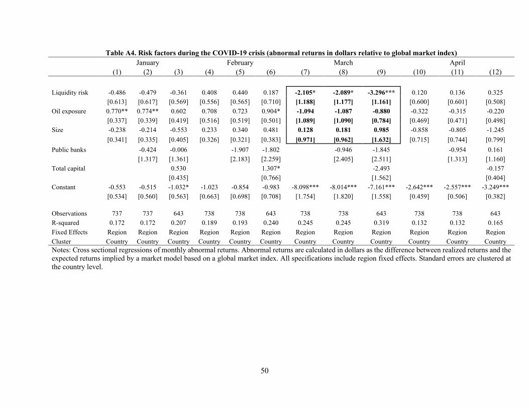
The decline in abnormal returns of less-liquid and more oil-exposed banks remained

unchanged from March to April (Panel D). By April, public banks experienced a large and

statistically significant drop in their abnormal returns of about 2.6 percentage points.

In addition, we estimate equation 2 using as dependent variable the excess returns of bank

stocks relative to their domestic market. This variable is calculated by subtracting the returns of

bank b’s domestic market from the bank’s returns (i.e., 𝐴𝐴𝑏𝑏,𝑡𝑡 − 𝐴𝐴𝑅𝑅𝑡𝑡).14 In Figure 3, we compare

the findings from estimating equation 2 using excess returns and the results with abnormal returns.

As Panel A shows, banks’ underperformance relative to their domestic market is more pronounced

for less liquid banks, banks more exposed to the oil sector and larger banks. However, the negative

returns of larger banks are not significant once we adjust for market risk. The returns of less liquid

banks and banks with more exposure to the oil industry were abnormally low, with the gap

continuing during April. Adjusting stock returns by market risk also reveals that public banks

enjoyed significant abnormal returns in March, although by April these had become negative, as

in the case of excess returns.15

Globally, banks entered the COVID-19 crisis better positioned to support the lending needs

of the real economy. As documented by the BIS, the capital and liquidity buffers of banks at the

onset of the crisis were substantially stronger than compared to the GFC (Borio, 2020; Lewrick et

al., 2020). Through aggressive interventions in the financial markets, governments have

encouraged banks to continue providing credit, in some cases by incentivizing them to draw down

their buffers. While this time banks appear to be part of the solution to the crisis, the banking sector

14 The results from this exercise are presented in Appendix Table A3. 15 We further calculate abnormal returns relative to a global index and using the Fama-French 3 factor model. The results from these exercises are displayed in Tables A4 and A5 of the Appendix.

15

has also been hit hard by a rapid increase in the amount of credit losses and an extended uncertainty

on the credit environment and duration of the crisis.

4. Measuring the market response to financial sector distress policy initiatives

What is the effectiveness of policy measures taken during the height of the crisis? To answer

this question, in this section we evaluate the market response to different policy initiatives

addressing the financial sector distress.

4.1. Policy interventions

We use data on the dates and types of major policy initiatives to support the financial sector

and address the impact of the COVID-19 emergency. The data were compiled and made publicly

available by the World Bank (World Bank, 2020). It covers policy measures in low, middle, and

high-income countries. Information on each policy measure was collected from national

authorities and international organizations. For each policy initiative, the dataset reports details on

the announcement, and the day (and not the hour or minute) of the announcement which restricts

our analysis to daily frequency. We classify approved measures that target the banking sector into

the following categories: (i) liquidity support, (ii) prudential measures, (iii) borrower assistance,

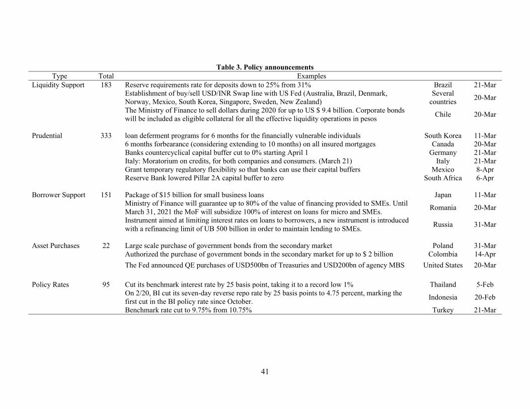
and (iv) monetary policy (Table 3).

Liquidity support deals with potential shortages in funding, either because precautionary

demand for liquidity has increased or because of lack of access to funding (e.g., wholesale funding

markets have dried up). Measures included are provisions of domestic currency liquidity through

broadened access to central bank refinancing, extended collateral framework, such as those in the

short-term and long-term repo market, and available foreign currency liquidity through swap

agreements between central banks.

16

Prudential measures include temporary relaxation of certain key regulatory and

supervisory requirements, including changes in capital requirements, limits on exposure,

concentration, loan-to-value ratios, minimum reserve requirements, and cancelation of stress tests.

By slowing down the decline in banks’ regulatory capital ratios, these measures reduce the rate at

which banks draw buffers down, spreading the recognition of losses and allowing a given amount

of equity to support a larger lending volume.

Borrower assistance include measures to supply funds to firms and households due to the

loss of revenue/income from the extended lockdowns. These include government liability

guarantees for newly issued or existing wholesale financing, direct credit lines to strategic sectors,

state support for interest-free loans and fully replenishable working capital financing. Other

measures include enhancement of deposit protection schemes and simplified programs of loan

restructuring.

Monetary policy are interest rate decisions (e.g., benchmark rate, repo rates, etc.), central

bank purchases of government securities (Quantitative Easing), and credit easing, which typically

consist of purchases of private sector debt in secondary markets. Given the different nature of

conventional and unconventional monetary policy measures, we further split this category into

Policy Rate announcements and Asset Purchases (both public and private bond buying programs

and purchases of asset-backed securities).

Our final sample contains policies in 17 developed and 28 developing countries, for which

we have stock market and policy data (Table 4). Some European countries such as, Austria,

Finland, and Netherlands, did not have domestic financial policy initiatives. We include banks of

these countries in days of announcements by the European Central Bank. Other Euro countries,

for example, France, Germany, Italy, and Spain have both financial support policies taken at the

17

country level in addition to those taken by the monetary union authorities.16 In total, the database

includes 389 announcements between February 1 and April 17. Prudential measures accounted for

the largest share of policy initiatives (36%), followed by borrower support, liquidity provision

measures, monetary policy and asset purchases (23%, 21%, 12% and 8% respectively). However,

the type of policies adopted differed substantially across countries (see Table A6 in the Appendix).

While monetary policy announcements were frequent in developing countries (representing 22%

of all measures), they only accounted for 4% in developed ones. In contrast, prudential measures

in developed countries constituted 43% of all announcements, compared to 26% in developing

countries.

Figure 4 presents the timing of policy announcements. Early in February, financial markets

and financial authorities had little reaction to the original outbreak in China and the ensuing

lockdown of Wuhan. On February 20, when Italy announced the quarantine of eleven

municipalities in the northern region, and once it was apparent that the outbreak had also spread

to South Korea, and Iran, stock markets declined sharply. By this date, only five countries had

taken financial sector policy interventions. Among these, Russia, Thailand, China and Indonesia

lowered their short-term interest rates and Japan launched a crisis loan package to small businesses.

Following a myriad of national quarantines starting with Italy on March 10, travel bans,

including the U.S. decision on March 12 to severely restrict travel from the EU, stock markets

around the world declined more than 30% from their peak. Interestingly, at this stage of the global

crisis, most financial authorities were only taking conventional monetary policy actions, reducing

short-term rates. For example, between February 20 and March 18, seventeen countries in our

16 We also include eight policy announcements that were made during weekends. For these cases, we study the stock response using the first business day when the domestic stock market opened.

18

sample had announced policy rate cuts, and only a few had either taken measures to assist

borrowers or announced prudential measures (e.g., Italy, Germany, U.K., and South Korea).

In response to the unprecedented, and rapidly evolving situation, policymakers increased

the scope and number of measures to support the financial system. After March 18, most

government and monetary authorities included liquidity support measures and borrower

assistance. For instance, by April 17, 35 countries had taken some measure of direct borrower

support, in most cases, dealing with SME financing. The use of countercyclical prudential rules

also became ubiquitous; by the end of our sample, 40 countries had introduced prudential actions,

typically through a temporary relaxation of certain key regulatory and supervisory requirements.

A large number of interventions were announced simultaneously with other financial sector

policies. For example, prudential measures in developed countries were often announced on the

same day of borrower support program announcements (Table A6 in the Appendix). However, as

Tables A6 shows, there were also multiple single policy announcements for each of the policy

categories we study. In developed countries, 42% of policies were announced on days with no

other financial sector program announcements. This share is higher among developing countries,

where 51% of policies were made on single announcement days.

4.2. Empirical methodology

We use an event study technique (Brown & Warner, 1996; Kothari & Warner, 2007) to

test the effect of policy announcements on the stock returns of banks. More specifically, we want

to assess whether different policy initiatives convey new information about the ability of banks to

properly operate during and after the crisis. Measuring bank-level stock returns instead of an

aggregate index of bank stocks prices (or interbank credit and liquidity risk premia), allows us to

19

exploit variation across banks to better understand the market response to different types of

policies.17 For example, the cross-sectional analysis allows us to answer whether a specific type

of government support measure favored a particular group of banks. Our focus is on the reaction

of stock prices, as opposed to bond yields, because stocks are more frequently traded than bonds.

Also, we do not use other bank-specific risk measures such as credit default swaps spreads, because

these securities are not widely available for the majority of banks in developing countries.

To assess the stock market reaction to a policy announcement, we compute the

accumulated abnormal stock returns of banks during the event. To be precise, we calculate

accumulated abnormal returns over an event window n, which is the variation in the stock price

one day prior to the announcement on day t, to n days after in excess to the expected returns implied

by the market model (𝐴𝐴𝐴𝐴𝐴𝐴𝐴𝐴𝑏𝑏,𝑡𝑡𝑛𝑛 ).

After calculating bank-level abnormal returns, we test whether policy announcements have

significant effects on bank stock returns. In our benchmark specification, we test this hypothesis

by estimating the following equation:

𝐴𝐴𝐴𝐴𝐴𝐴𝐴𝐴𝑏𝑏,𝑐𝑐,𝑡𝑡𝑛𝑛 = 𝛼𝛼0,𝑛𝑛 + 𝛼𝛼1,𝑛𝑛𝐼𝐼𝑂𝑂𝐿𝐿𝐿𝐿𝑏𝑏 + 𝛼𝛼2,𝑛𝑛𝑂𝑂𝐿𝐿𝑂𝑂𝑏𝑏 + 𝛼𝛼3,𝑛𝑛𝑆𝑆𝐿𝐿𝑆𝑆𝐴𝐴𝑏𝑏 + 𝛼𝛼4,𝑛𝑛𝑃𝑃𝐿𝐿𝑃𝑃𝑂𝑂𝐿𝐿𝑃𝑃𝑏𝑏 + 𝛾𝛾𝑐𝑐 + 𝛾𝛾𝑡𝑡 + 𝐿𝐿𝑏𝑏,𝑐𝑐,𝑡𝑡 (3)

where 𝐴𝐴𝐴𝐴𝐴𝐴𝐴𝐴𝑏𝑏,𝑐𝑐,𝑡𝑡𝑛𝑛 represents the abnormal return of bank b located in country c in day t, measured

over the [-1, n] window (in days). The covariates are bank observables which include, bank

illiquidity, oil exposure, and the indicator that captures whether the bank has state ownership.

Finally, 𝛾𝛾𝑐𝑐 and 𝛾𝛾𝑡𝑡 are country and announcement date fixed effects. Standard errors are clustered

at the country level.

17 Correa et al. (2014) also use bank stock prices to evaluate another kind of shock – the downgrade of the sovereign credit risk.

20

We estimate equation (1) separately for each policy category. Since bank illiquidity, oil

exposure, and bank size variables are standardized, the constant 𝛼𝛼0,𝑛𝑛 captures the abnormal stock

returns of the average private bank for a type of announcement in the [-1, n] window. The

coefficients 𝛼𝛼1,𝑛𝑛, 𝛼𝛼2,𝑛𝑛, 𝛼𝛼3,𝑛𝑛 and 𝛼𝛼4,𝑛𝑛 capture cross-sectional differences in the response of bank

stock prices. For example, 𝛼𝛼1,𝑛𝑛 > 0 would suggest that illiquid banks have higher accumulated

abnormal returns than liquid banks during the event window for a specific type of announcement.

There are several challenges to our identification. First, owing to the high degree of global

financial integration, there is extensive evidence of international spillovers from policy

announcement by systemically important countries (Ait-Sahalia et al., 2012; Morais et al., 2019).

To avoid contaminating the analysis from the effects of financial policy initiatives taken by core

countries, we exclude data from days when the U.S. or European authorities made major

announcements covering the same broad policy type category. For example, on a day when the

U.S. authorities announced liquidity support measures, we keep data from stock returns of U.S.

banks in the sample but exclude banks in countries that issue liquidity announcement on the same

day.

Second, due to the nature and scale of the crisis, in some cases, national government

authorities announced multiple financial measures during the same day. In such situations, and

without intraday time stamp for each announcement category, it is difficult to disentangle the effect

of each policy on bank stock prices. To deal with these confounding factors, we further condition

our sample to country-dates where only policies of a particular category were announced, and

report results for this restricted sample.

21

Finally, selecting the length of the event window has important tradeoffs. Limiting the size

of the window helps to avoid contaminating the analysis of a given announcement’s effect with

other news; particularly in a period when pandemic-related news was heightened. If the event

window is too narrow, there might not be enough time for market participants to internalize the

context and implications of complex policy announcements. This is likely to be more pronounced

in developing countries, where trading volume in secondary markets is small and the speed of

transactions is slower (e.g., the pace of business at which risk is transferred across market

participants is longer).18 In turn, we use a five-day window, evaluating the change in stock prices

from one day before the announcement to three days after, that is, n = {0,1,2,3}. We report

accumulated abnormal returns for every day during this time window.

4.3. Impact of policy announcements

As a benchmark to gauge the magnitude of the stock market effects, we first plot the

average abnormal returns during the event window for each policy category, pooling banks across

all countries. Abnormal returns are obtained from estimating equation (3) on a constant, removing

all other covariates and using day and country fixed effects. The results are displayed in Figure 5

for the full sample (Panel A) and the restricted sample (Panel B) – when announcements of a

particular category do not overlap with other initiatives. During our sample period, borrower

assistance initiatives were strongly associated with large increases in the abnormal returns of bank

stocks during the announcement day; 146 bps and 199 bps in the full and restricted sample

respectively. We find that these large excess returns are present up to three days after the

18 See for example Pedraza et al, (2019).

22

announcement. Borrower assistance initiatives typically include the introduction of government

guarantees, which automatically transfer risks from banks’ balance sheets to the sovereign.

On days when prudential measures and policy rate reductions were announced, bank stocks

display positive but small abnormal returns in the full sample (45bps and 39bps respectively).

These returns are quickly reversed within two days after the policy initiatives were announced.

Notably, when we restrict the sample to single policy announcements, prudential measures seem

to be accompanied by immediate price drops in bank stocks; 128 bps during the announcement

day.19 Prudential policies allow banks to run down some of their buffers to absorb the shock and

send a strong signal about the resolve of policymakers. However, the fact that bank stock returns

are negative might suggest that markets are also pricing the downside risk from the depletion of

capital buffers.

Finally, we do not find evidence that liquidity support announcements had any aggregate

short-term effects on bank stock prices. Although bank stocks seem to display positive abnormal

returns when liquidity assistance measures are combined with other policies (Panel A in Figure 5),

in the restricted sample, abnormal returns are small and statistically indistinguishable from zero.

The results on the cross-sectional impact of financial sector policies are presented in Table

5 and Figure 6.20 While we present findings for the full and restricted sample, our preferred

specification and discussion focuses on single policy initiatives. The constant in each model

19 As Table A6 shows, in developed countries, 35 of the 99 prudential policy measures were jointly announced with borrower assistance initiatives. This might explain why in the full sample the net effect of prudential policies is higher than in the restricted sample. 20 To present all the policies in a single table, we only include same-day estimates (n=0) and three days after the announcement (n=3). However, the figures display estimates during the entire event window.

23

represents the average abnormal returns of private banks in the sample. The results confirm our

previous finding that borrower assistance measures are strongly associated with banks’ stock price

response. Other policy initiatives seem to have smaller or even negative aggregate effects on bank

stocks.

4.3.1 Liquidity Support

Announcements of liquidity support are strongly associated with a reduction in the liquidity

premium. That is, stocks of less liquid banks overperform after policymakers announce liquidity

and funding measures. The coefficient for the liquidity premium can be read as follows: a bank

with a liquidity premium measure of one-standard deviation higher than the average, experienced

an additional 64 bps of abnormal returns on days when the government announced liquidity

support policies (193 bps of abnormal returns accumulated over a four day window). The result is

important because it confirms that central banks action helped alleviate the sharp tightening of

financial conditions at the onset of the crisis. During March, due to the overwhelming volatility in

securities and FX markets, many financial entities reported having difficulties in accessing

funding, which is consistent with the sharp increase the liquidity premium in that month

documented in Section 3. Overall, policies targeting funding availability (whether in domestic or

foreign currency) appear to have a favorable impact in the reduction of the liquidity risk premium.

We also see that stock prices of public banks and those of smaller banks benefit more from liquidity

measures, potentially due to greater reductions in uncertainty these policies provide to these banks.

4.3.2 Prudential measures

In addition to having a negative impact on aggregate bank stock prices, prudential measures

do not seem to be associated with clear reductions in the liquidity premium. The use of buffers,

24

facilitation of loan restructuring, and other measures that require regulatory forbearance (e.g., loan

moratoria and different treatment of non-performing loans), might help support credit flow

throughout the lockdowns, but they entail large risks in the medium term, threatening financial

stability. It appears that markets are pricing these risks, since abnormal returns are negative.

Furthermore, our evidence indicates that the effect of prudential measures is undistinguishable

across banks, irrespective of their liquidity ratios and exposure to the oil sector. Our results suggest

that stocks of larger banks displayed higher abnormal returns after prudential measures were

announced, although the magnitude of this effect is small and only statistically significant on the

announcement day.

4.3.3 Borrower assistance

Announcements of borrower assistance were associated with large increases in abnormal

returns of bank stocks. Recognizing the severity of the shock, especially to small non-essential

businesses that would be unable to cover operating costs during extended lockdowns, many

countries enhanced their public liability guarantees programs, with government guarantees up to

90% of loan values. Fiscal resources were also committed to subsidize interest-free loans and

directly fund strategic sector during the pandemic. These initiatives generate large fiscal costs in

the short term, while transferring the credit risks from banks to the government. It appears that

markets internalize this information as good news for the banking industry, which could now

offload part of the burden of the shock to the sovereign.

Announcements of borrower support programs had a greater impact among less liquid

banks. Concretely, three days after an announcement, the abnormal returns of a bank with a

liquidity ratio one-standard deviation below the mean increase in 87bps. Additionally, larger banks

experience higher abnormal returns during borrower support announcements. For instance, a bank

25

that is one-standard deviation above the mean in size, experiences an additional 98bps of abnormal

returns up to three days after the announcement. Ornelas et al., (2019) document that during the

GFC, large banks disproportionally benefited from allocating government-sponsored credit. While

loans that are funded with government resources typically have interest rate ceilings, banks offset

the lower revenue from these loans by extracting rents in other lending products to the recipients

of government support. Smaller banks and those that operate in niche markets are less able to take

advantage of cross-selling and enhanced sales in other products.

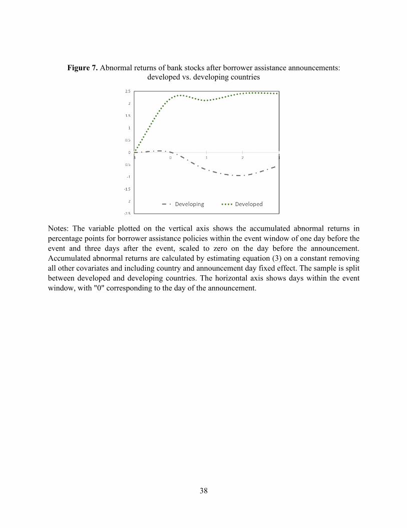
When we split the sample into developed and developing countries, we find that the

positive association between excess stock returns and borrower support initiatives are exclusive to

developed countries (see Table 6 and Figure 6). As noted above, borrower assistance requires

potentially large fiscal commitments. In developing countries, authorities have lower fiscal space

to operate, and markets might anticipate that the extent of the borrower assistance measures in

such settings is limited. On the contrary, fiscal authorities in developed countries can pledge

significant resources to help distressed households and firms, which in turn reduce bank risk.

4.3.3 Monetary policy

Interest rate cuts were associated with significant declines in the liquidity risk premium.

To be precise, during days of policy rate cuts, banks with lower liquidity experienced higher

abnormal returns than more liquid banks (full and restricted sample in Table 5). The significant

relative increase in abnormal stock returns of illiquid banks may have reflected markets’

expectation that lower interest rates would increase liquidity in the financial system, thereby

benefiting banks with larger funding risks. The result also confirms that the interest rate policy

remained a key policy tool at the onset of the crisis, since markets are familiar with conventional

monetary policy.

26

Banks with more exposure to the oil shock seem to benefit less from interest rate actions,

as evidenced in both the full and restricted sample. The result highlights the key difference between

liquidity and solvency risks. Banks that are heavily exposed to the oil sector are more susceptible

to losses due to the likelihood of defaults in this industry. To the extent that markets internalize

that the profitability of these banks will be lower, interest rate cuts would have small effects. On

the other hand, banks with short-term liquidity constraints, but with less exposed portfolios, stand

to benefit more from the ease in funding conditions.

Announcement concerning asset purchases were also followed by increases in the

abnormal returns of illiquid banks, albeit with marginal statistical significance in the restricted

sample. We interpret this finding as evidence that unconventional monetary policy also played a

role in reducing the liquidity risk premium.

Since announcements should have a greater impact if they are unexpected than if they are

expected, we further restrict our sample to days with monetary policy surprises. That is, we restrict

our sample to days when the monetary authority made policy rate announcements after emergency

meetings, or when the domestic policy rate cut was larger than the expected by market analysts.21

We further confirm earlier findings with the sample of unexpected monetary policy

announcements. Although surprises of interest rate cuts were not associated with significant

increases in bank stock prices, such announcements did appear to have differential effect across

banks. For instance, monetary policy surprises were associated with declines in the liquidity risk

21 According to the Reuters forecast based on the one-week analyst survey of benchmark rates. Some examples of monetary policy surprises include Thailand’s 25bps cut in the benchmark rate (February 5), Canada’s repo rate cut of 50bps (March 4), and the United Kingdom 50bps repo rate cut during the emergency meeting of March 11. The only case in which the rate cut was smaller than expected was in Thailand on March 20. We drop this date from the sample of monetary policy surprises.

27

premium and seemed to be more beneficial for banks with lower exposure to the oil sector (Table

A7 in the Appendix).

5. Conclusions

The spread of COVID-19 represents an unpresented global shock, with the disease itself

and mitigation efforts –such as social distancing measures and partial and national lockdowns

measures– both having a significant impact on the economy. In the immediate aftermath, the

financial sector, particularly banks, were expected to play an important role in absorbing the shock

by supplying vital credit to the corporate sector and households. In an effort to facilitate this,

central banks and governments around world enacted a wide range of policy measures to provide

greater liquidity and support the flow of credit. An important policy question is the potential

impact of these countercyclical lending policies on the future stability of the banking systems and

to what extent their strengthened capital positions since the global financial crisis will allow them

to absorb this shock without undermining their resilience.

In this paper, we use daily stock prices and other balance sheet information for a sample of

banks in 53 countries to take a first look at this issue. Our contribution is twofold. We first assess

the impact of the pandemic on the banking sector and investigate whether the shock had a

differential impact on banks versus corporates, as well as those banks with different characteristics.

Second, using a global database of financial sector policy responses and an event study

methodology, we investigate the role of different policy initiatives on addressing bank stress as

perceived by markets, in the aggregate, as well as across different banks.

Our results suggest that the adverse impact of the COVID-19 shock on banks was much

more pronounced and long-lasting than on the corporates as well as other non-bank financial

28

institutions, revealing the expectation that banks are to absorb at least part of the shock to the

corporate sector. Furthermore, larger banks, public banks, and to some extent better capitalized

banks suffered greater reductions in their stock returns, reflecting their greater anticipated role in

dealing with the crisis. Banks with lower pre-crisis liquidity and oil sector exposure also suffered

greater reduction in returns, consistent with their greater vulnerability to such a shock.

Investigating close to 400 policy announcements between February and April 2020, we

next evaluate the impact of liquidity support, prudential measures, borrower assistance and

monetary policy measures on bank abnormal returns. Our results suggest liquidity support and

borrower assistance measures had the greatest positive impact on bank abnormal returns. Illiquid

banks benefited most from liquidity support, whereas larger banks and public banks saw increased

abnormal returns with the announcement of borrower assistance policies. However, since they

rely on fiscal expenditures, these policies did not result in positive impact on bank stock prices in

developing countries where there is less room for fiscal expansion. Prudential measures appeared

to have a negative impact on bank returns, suggesting that markets price the downside risk from

depletion of capital buffers. Finally, policy rate cuts and assets purchases mostly benefited illiquid

banks and public banks, confirming that monetary policy again played a key tool during this crisis.

Overall, our results suggest that the crisis and the countercyclical lending role they are

expected to play has put banking systems around the world under stress, having a differential

impact depending on their characteristics and pre-crisis vulnerabilities. While some policy

measures such as liquidity support, borrower assistance and monetary easing moderated this

adverse impact for some banks, this is not true for all banks or in all circumstances. For example,

borrower assistance measures exacerbated the stress for banks that operate in countries with little

29

fiscal space. These vulnerabilities will need to be carefully monitored in the coming year as the

pandemic continues to take its toll on the world economies.

30

References Acharya, V., & Steffen, S. (2020). The risk of being a fallen angel and the corporate dash for cash in the

midst of COVID. CEPR COVID Economics, 10.

Ait-Sahalia, Y., Andritzky, J., Jobst, A., Nowak, S., & Tamirisa, N. (2012). Market response to policy initiatives during the global financial crisis. Journal of International Economics, 87, 162-177.

Baker, S., Bloom, N., Davis, S., & Terry, S. (2020). Covid-induced economic uncertainty. National Bureau of Economic Research.

Borio, C. (2020). The prudential response to the Covid-19 crisis. Bank of International Settlements.

Brown, S. J., & Warner, J. B. (1996). Using daily stock returns: The case of event studies. Journal of Financial Economics(14), 3-31.

Claessens, S., Klingebiel, D., & Laeven, L. (2005). Ciris resolution, policies, and institutions: empirical evidence. In Systemic Financial Distress: Containment and Resolution. Cambridge: Cambridge University Press.

Correa, R., Lee, K.-H., Sapriza, H., & Suarez, G. (2014). Sovereign credit risk, banks' government support, and bank stock returns around the world. Journal of Money, Credit and Banking, 46(1), 93-121.

Drehmann, M., Farag, M., Tarashev, N., & Tsatsaronis, K. (2020). Buffering Covid-19 losses: The role of prudential policy. Bank of International Settlements.

Fama, E., & French, K. (1993). Common risk factors in the returns of stocks and bonds. Journal of Financial Economics, 81(3), 3-56.

Gormsen, N., & Koijen, R. S. (2020). Coronavirus: Impact on stock prices and growth expectations. University of Chicago, Becker Friedman Institute of Economics Working Paper.

Guerrieri, V., Lorenzoni, G., Straub, L., & Wening, I. (2020). Macoeconomic implications of COVID-19: Can negative supply shocks cause demand shortages? National Bureau of Economic Research.

Karolyi, A., & Stulz, R. (2003). Are financial assets priced locally or globally? In Handbook of the Econoimcs of Finance (pp. 975-1020). Amsterdam: Elsevier.

Kothari, S. P., & Warner, J. B. (2007). Econometrics of event studies. In Handbook of empirical corporate finance (pp. 3-36). Elsevier.

Landier, A., & Thesmar, D. (2020). Earnings expectations in the covid crisis. National Bureau of Economic Research.

Morais, B., Peydro, J.-L., & Roldan Peña, J. O.-R. (2019). The international bank lending channel of monetary policy. Journal of Finance, 74(1), 55-90.

Ornelas, J. R., Pedraza, A., Ruiz-Ortega, C., & Silva, T. (2019). Winners and losers when private banks distribute government loans. World Bank.

31

Pedraza, A., Pulga, F., & Vasquez, J. (2019). Costly index investing in foreign markets. Journal of financial markets, https://doi.org/10.1016/j.finmar.2019.100509.

Ramelli, S., & Wagner, A. (2020). Feverish stock price reactions to covid-19.

Reinhart, C. M., & Rogoff, K. S. (2009). This time is different: Eight centuries of financial folly. Princeton University Press.

Taylor, J., & Williams, J. (2009). A black swan in the money market. American Economic Journal: Macroeconomics, 1(1), 58-83.

World Bank, G. (2020, June 16). Covid-19 finance sector related policy responses. Retrieved from https://datacatalog.worldbank.org/dataset/covid-19-finance-sector-related-policy-responses

32

Figure 1. Average Stock Returns of Banks vs Firms and Non-Bank Financial Companies

Notes: The figures plot average daily stock market returns of banks, firms and non-bank financials in the sample normalized to January 1, 2020. The average returns of firms in the first figure are equally weighted across countries and are net from bank returns. To calculate them, we exclude the returns of banks from the returns of each country’s stock market using the index weights of banks. The average returns of banks are weighted by the contribution of each bank to the total bank assets of each region. The regional average bank returns are then equally weighted across regions. The same approach is used to obtain the average return of non-bank financials.

6070

8090

100

1/1/2020 2/1/2020 3/1/2020 4/1/2020 5/1/2020date

Firms Banks

Panel A. Banks vs Firms

6070

8090

100

1/1/2020 2/1/2020 3/1/2020 4/1/2020 5/1/2020date

Non-Bank Financials Banks

Panel B. Non-Bank Financials vs Banks

33

Figure 2. Average Stock Returns by Bank Characteristics

Notes: The figures plot average daily stock returns of all banks in the sample normalized to January 1, 2020. We classify banks according to their ownership as well as their 2019Q1-2019Q4 average liquidity, degree of exposure to the oil sector, total assets and Tier 1 capital ratio. Banks are classified as public-owned if the government has equity participation in them, and private otherwise. We split banks into below and above the median of their 2019Q1-2019Q4 averages of liquidity, size and Tier 1 capital. Banks are considered highly exposed to the oil sector if their degree of exposure is above the 75th percentile exposure. For each group of banks, we weight the average stock returns by the contribution of every bank to the bank assets of the group within a region. The regional average bank returns are then equally weighted across regions.

5060

7080

9010

0

1/1/2020 2/1/2020 3/1/2020 4/1/2020 5/1/2020date

Private Banks Public Banks

Panel A. Public vs Private Banks

5060

7080

9010

0

1/1/2020 2/1/2020 3/1/2020 4/1/2020 5/1/2020date

Low High

Panel B. Banks with Low vs High Liquidity

5060

7080

9010

0

1/1/2020 2/1/2020 3/1/2020 4/1/2020 5/1/2020date

Low Exposure High Exposure

Panel C. Banks with Low vs High Oil Exposure

6070

8090

100

110

1/1/2020 2/1/2020 3/1/2020 4/1/2020 5/1/2020date

Small Large

Panel D. Small vs Large Banks

5060

7080

9010

0

1/1/2020 2/1/2020 3/1/2020 4/1/2020 5/1/2020date

Below median Above median

Panel E. Banks below vs above Median Tier 1 Capital

34

Figure 3. Risk factors estimated by month Panel A. Excess Returns Panel B. Abnormal returns

Notes: Coefficients from monthly cross-sectional regression on excess stock returns (Panel A) and abnormal returns (Panel B) of banks. Liquidity risk, oil exposure, and size are standardized. “Public banks” is a dummy variable equal to 1 if the bank is state-owned and zero otherwise. Regressions include regional fixed effects with standard errors clustered at the country level.

35

Figure 4. Timeline of policy announcements

Notes: Number of countries with at least one policy announcement (by category).

36

Figure 5. Abnormal returns of bank stocks around the announcement window Panel A. Full sample Panel B. Restricted sample

Notes: The variable plotted on the vertical axis shows the accumulated abnormal returns in percentage points within the event window of one day before the event and three days after the event, scaled to zero on the day before the announcement. Accumulated abnormal returns are averaged across banks for each policy category. The horizontal axis shows days within the event window, with "0" corresponding to the day of the announcement.

37

Figure 6. Cross-sectional impact of policy announcements (in percentage points)

Notes: Estimated slope coefficients of OLS regressions estimating daily accumulated abnormal returns on bank characteristics. Liquidity risk, oil exposure, and Size are standardized. “Public banks” is a dummy variable equal to 1 if the bank is state-owned and zero otherwise. The horizontal axis shows days within the event window, with "0" corresponding to the day of the announcement.

38

Figure 7. Abnormal returns of bank stocks after borrower assistance announcements: developed vs. developing countries

Notes: The variable plotted on the vertical axis shows the accumulated abnormal returns in percentage points for borrower assistance policies within the event window of one day before the event and three days after the event, scaled to zero on the day before the announcement. Accumulated abnormal returns are calculated by estimating equation (3) on a constant removing all other covariates and including country and announcement day fixed effect. The sample is split between developed and developing countries. The horizontal axis shows days within the event window, with "0" corresponding to the day of the announcement.

39

Table 1. Summary statistics of banks Variable Mean SD P25 P50 P75 Obs Stock returns -0.004 0.003 -0.005 -0.003 -0.002 896 Public-owned bank 0.12 0.32 0.00 0.00 0.00 880 Liquidity ratio 0.14 0.47 0.02 0.07 0.11 755 Assets (IHS) 24.0 2.2 22.2 24.0 25.3 767 Tier 1 capital ratio 14.6 5.8 11.8 13.3 16.2 583 Total capital ratio 16.0 6.1 13.1 14.9 17.8 651 Exposure to oil sector 0.06 1.23 -0.22 0.02 0.23 894 Notes: The table presents summary statistics of the 896 banks across the 53 countries in the sample. Stock returns for each bank are averaged over the period January 1, 2020 to May 5, 2020. Assets, liquidity, capital ratios and exposure to the oil sector are calculated using data prior to COVID-19 (from 2019Q1 to 2019Q4). Assets correspond to the average total assets of a bank over time and are measured using the inverse hyperbolic sine (IHS) function. We define liquidity as the average ratio of cash and equivalents kept by a bank over its total assets. Tier 1 capital and Total capital ratios are the average regulatory ratios reported by banks. To measure the degree of exposure of a bank to the oil sector, we run an OLS regression of the bank's daily stock returns as a function of a constant term, the market return where the bank is located and the returns of oil prices for the period May 1, 2018 to December 31, 2019. The exposure to the oil sector of each bank is given by the coefficient of the return of oil prices in this regression.

40

Table 2. Risk factors during the COVID-19 crisis Panel A. January Panel B. February Panel C. March Panel D. April (1) (2) (3) (4) (5) (6) (7) (8) (9) (10) (11) (12) Liquidity risk -0.703 -0.714 -0.631 0.387 0.380 -0.059 -2.166** -2.241** -3.495*** -0.747* -0.702 -0.790 [0.581] [0.585] [0.550] [0.336] [0.348] [0.370] [0.933] [0.926] [0.903] [0.434] [0.424] [0.482] Oil exposure 0.740* 0.735* 0.588 0.214 0.211 0.622 -2.151** -2.185** -1.420* -0.042 -0.021 -0.110 [0.377] [0.376] [0.477] [0.408] [0.406] [0.403] [1.046] [1.050] [0.752] [0.388] [0.393] [0.427] Size -0.086 -0.124 -0.458 0.516 0.494 0.724* 1.013 0.771 2.047* -0.499 -0.352 -0.730 [0.382] [0.379] [0.461] [0.378] [0.362] [0.373] [0.636] [0.631] [1.013] [0.622] [0.606] [0.765] Public banks 0.675 1.185 0.394 0.338 4.360 3.512 -2.635** -2.174* [1.163] [1.230] [2.129] [2.217] [2.918] [3.272] [1.177] [1.129] Total capital 0.316 0.717* -2.111 -0.095 [0.438] [0.389] [1.381] [0.413] Constant -1.416*** -1.476*** -1.864*** 0.064 0.029 0.000 -6.644*** -7.030*** -6.359*** -3.197*** -2.964*** -3.355*** [0.502] [0.538] [0.567] [0.373] [0.419] [0.410] [1.502] [1.567] [1.352] [0.562] [0.555] [0.491] Observations 737 737 643 738 738 643 738 738 643 738 738 643 R-squared 0.089 0.089 0.107 0.060 0.061 0.087 0.104 0.110 0.163 0.023 0.027 0.029 Fixed Effects Region Region Region Region Region Region Region Region Region Region Region Region Cluster Country Country Country Country Country Country Country Country Country Country Country Country Notes: Cross sectional regressions of monthly abnormal returns of banks. Abnormal returns are the difference between realized returns and the expected returns implied by a market model. All specifications include region fixed effects. Standard errors are clustered at the country level.

41

Table 3. Policy announcements Type Total Examples

Liquidity Support 183 Reserve requirements rate for deposits down to 25% from 31% Brazil 21-Mar

Establishment of buy/sell USD/INR Swap line with US Fed (Australia, Brazil, Denmark, Norway, Mexico, South Korea, Singapore, Sweden, New Zealand)

Several countries 20-Mar

The Ministry of Finance to sell dollars during 2020 for up to US $ 9.4 billion. Corporate bonds will be included as eligible collateral for all the effective liquidity operations in pesos Chile 20-Mar

Prudential 333 loan deferment programs for 6 months for the financially vulnerable individuals South Korea 11-Mar 6 months forbearance (considering extending to 10 months) on all insured mortgages Canada 20-Mar Banks countercyclical capital buffer cut to 0% starting April 1 Germany 21-Mar Italy: Moratorium on credits, for both companies and consumers. (March 21) Italy 21-Mar Grant temporary regulatory flexibility so that banks can use their capital buffers Mexico 8-Apr Reserve Bank lowered Pillar 2A capital buffer to zero South Africa 6-Apr Borrower Support 151 Package of $15 billion for small business loans Japan 11-Mar

Ministry of Finance will guarantee up to 80% of the value of financing provided to SMEs. Until March 31, 2021 the MoF will subsidize 100% of interest on loans for micro and SMEs. Romania 20-Mar

Instrument aimed at limiting interest rates on loans to borrowers, a new instrument is introduced with a refinancing limit of UB 500 billion in order to maintain lending to SMEs. Russia 31-Mar

Asset Purchases 22 Large scale purchase of government bonds from the secondary market Poland 31-Mar Authorized the purchase of government bonds in the secondary market for up to $ 2 billion Colombia 14-Apr

The Fed announced QE purchases of USD500bn of Treasuries and USD200bn of agency MBS United States 20-Mar Policy Rates 95 Cut its benchmark interest rate by 25 basis point, taking it to a record low 1% Thailand 5-Feb

On 2/20, BI cut its seven-day reverse repo rate by 25 basis points to 4.75 percent, marking the first cut in the BI policy rate since October. Indonesia 20-Feb

Benchmark rate cut to 9.75% from 10.75% Turkey 21-Mar

42

Table 4. Number of days with policy announcements

Country First date Last date Liquidity Prudential Borrower Support

Asset Purchases

Policy Rates

Argentina 5-Mar 5-Apr 1 1 2 0 1 Australia 1-Mar 17-Apr 2 6 0 0 2 Austria 12-Mar 16-Apr 3 7 4 2 0 Brazil 2-Mar 16-Apr 7 5 3 0 1 Bulgaria 19-Mar 15-Apr 1 2 4 0 0 Canada 4-Mar 15-Apr 0 3 0 2 3 Chile 20-Mar 20-Mar 1 0 1 0 1 China 20-Feb 15-Apr 2 1 2 0 3 Colombia 20-Mar 16-Apr 3 1 1 2 1 Croatia 20-Mar 31-Mar 1 0 1 0 0 Egypt 24-Mar 16-Apr 0 2 1 0 0 Finland 12-Mar 16-Apr 3 7 4 2 0 France 12-Mar 16-Apr 3 10 6 2 0 Germany 12-Mar 16-Apr 3 9 6 2 0 Hong-Kong 4-Mar 18-Apr 0 3 1 0 2 India 20-Mar 17-Apr 5 2 1 0 2 Indonesia 20-Feb 14-Apr 2 1 0 1 2 Ireland 12-Mar 16-Apr 3 7 4 2 0 Italy 1-Mar 16-Apr 3 9 7 2 0 Japan 20-Feb 15-Apr 0 2 2 0 1 Malaysia 3-Mar 27-Mar 2 1 1 0 1 Mexico 12-Mar 15-Apr 3 4 1 0 1 Morocco 17-Mar 27-Mar 1 1 0 0 1 Netherlands 12-Mar 16-Apr 3 7 4 2 0 Nigeria 18-Mar 20-Mar 1 1 2 0 0 Pakistan 17-Mar 16-Apr 1 1 1 0 3 Peru 19-Mar 17-Apr 2 2 3 0 1 Philippines 20-Mar 16-Apr 2 0 0 1 2 Poland 20-Mar 8-Apr 1 1 1 1 2 Portugal 12-Mar 16-Apr 3 7 4 2 0 Qatar 10-Mar 10-Mar 0 0 0 0 1 Romania 20-Mar 9-Apr 2 2 1 1 1 Russia 7-Feb 17-Apr 1 4 1 0 1 Saudi-Arabia 10-Mar 16-Mar 0 0 0 0 2 Singapore 16-Apr 16-Apr 0 1 0 0 0 South-Africa 19-Mar 14-Apr 2 5 1 1 2 South-Korea 11-Mar 13-Apr 2 6 3 0 1 Spain 12-Mar 16-Apr 3 8 5 2 0 Sweden 6-Apr 14-Apr 2 0 0 0 0 Thailand 5-Feb 20-Mar 0 1 0 0 2 Turkey 17-Mar 17-Apr 2 1 1 1 1 UAE 10-Mar 10-Mar 0 0 0 0 1 UK 11-Mar 17-Apr 2 4 6 1 2 US 15-Mar 17-Apr 5 6 2 1 1 Vietnam 17-Mar 17-Apr 0 0 2 0 1

Notes: Data obtained from the World Bank (World Bank, 2020) covering the period February 1 to April 17 2020.

43

Table 5. Impact of policy initiatives Liquidity Support Prudential Meas. Borrower Assist. Asset Purchases Policy Rates All announcements n = 0 3 0 3 0 3 0 3 0 3 0 3

Full sample: days with multiple domestic policy announcements Liquidity risk 0.713*** 0.999** 0.295* 0.364 0.348** 0.509* 0.463 2.215*** 0.744** 1.369*** 0.373*** 0.711*** [0.267] [0.455] [0.173] [0.292] [0.159] [0.299] [0.360] [0.734] [0.291] [0.513] [0.116] [0.206] Oil exposure 0.187 0.153 0.065 0.337 0.143 -0.267 -0.579 0.832 -0.505*** -0.901*** -0.090 -0.094 [0.180] [0.310] [0.143] [0.244] [0.174] [0.344] [0.391] [0.807] [0.180] [0.315] [0.096] [0.173] Size -0.002 -0.554* 0.321** 0.218 0.793*** 0.656* -0.874** -1.925** 0.145 0.145 0.305*** 0.081 [0.191] [0.328] [0.136] [0.235] [0.184] [0.353] [0.404] [0.830] [0.263] [0.457] [0.101] [0.184] Public banks 0.550 0.392 -0.755 0.042 -0.065 0.959 1.836** 0.523 -0.362 1.485* 0.030 0.194 [0.533] [0.903] [0.502] [0.846] [0.628] [1.162] [0.917] [1.876] [0.464] [0.807] [0.301] [0.532] Constant 1.598*** 0.725** 0.419*** -0.234 1.314*** 1.272*** 0.051 0.428 0.532** -0.749* 0.536*** -0.021 [0.187] [0.318] [0.132] [0.223] [0.131] [0.250] [0.344] [0.715] [0.236] [0.415] [0.082] [0.147] Observations 774 762 1,348 1,319 573 558 115 113 377 373 2,408 2,358 R-squared 0.292 0.484 0.364 0.452 0.426 0.248 0.171 0.269 0.268 0.258 0.323 0.338

Restricted sample: days with single domestic policy announcements Liquidity risk 0.643 1.929** 0.077 0.156 0.546*** 0.866** 0.326 1.867* 0.537* 1.415*** 0.321** 0.786*** [0.466] [0.948] [0.208] [0.356] [0.199] [0.365] [0.505] [0.966] [0.281] [0.463] [0.125] [0.227] Oil exposure -0.217 -1.037* -0.214 0.194 0.123 -0.059 -0.279 -0.519 -0.632*** -0.816*** -0.280*** -0.376* [0.273] [0.554] [0.194] [0.335] [0.202] [0.392] [0.853] [1.635] [0.181] [0.297] [0.106] [0.197] Size -0.948** -2.423*** 0.425** 0.435 0.903*** 0.978** -0.646 -4.243** 0.403 0.458 0.349*** 0.118 [0.372] [0.756] [0.174] [0.310] [0.213] [0.398] [0.820] [1.585] [0.268] [0.434] [0.115] [0.215] Public banks 1.440** 0.707 -0.828 -1.827 0.394 0.030 1.254 0.905 0.306 1.240 0.254 -0.162 [0.625] [1.268] [0.725] [1.250] [0.948] [1.694] [1.624] [3.107] [0.525] [0.852] [0.334] [0.602] Constant -0.087 0.631 -1.217*** -1.388*** 1.849*** 1.957*** 0.607 1.436 -0.009 -1.309*** -0.129 -0.458*** [0.364] [0.741] [0.155] [0.265] [0.153] [0.282] [0.627] [1.233] [0.243] [0.400] [0.090] [0.164] Observations 189 188 711 693 446 431 51 50 286 282 1,688 1,649 R-squared 0.306 0.389 0.282 0.389 0.398 0.232 0.134 0.431 0.339 0.296 0.336 0.290 Notes: The table presents the estimates of cross-sectional regressions of the impact of financial sector policies on the excess returns of banks on announcement days (n=0) and three days after the announcement (n=3). Excess returns are calculated as the bank stock returns during the month minus the returns of the domestic stock market index. All specifications include region fixed effects. Standard errors are clustered at the country level.

44

Table 6. Heterogeneity in the impact of policy initiatives (developed vs developing countries) Liquidity Support Prudential Meas. Borrower Assist. Asset Purchases Policy Rates All announcements n = 0 3 0 3 0 3 0 3 0 3 0 3

Developed Countries Liquidity risk 0.324 1.431 0.025 0.146 0.530** 0.878** 0.422 1.928* -0.396 5.330** 0.252* 0.731*** [0.482] [0.924] [0.222] [0.378] [0.207] [0.375] [0.532] [1.077] [1.246] [2.291] [0.142] [0.257] Oil exposure -0.187 0.294 -0.089 0.407 0.115 -0.313 -1.199 -1.634 -0.078 -8.749** -0.034 0.065 [0.673] [1.291] [0.207] [0.356] [0.213] [0.406] [1.088] [2.212] [2.211] [4.065] [0.146] [0.271] Size -0.785 -3.446*** 0.563*** 0.702** 0.971*** 1.161*** -1.074 -4.299** 2.043* -0.305 0.635*** 0.628** [0.527] [1.011] [0.185] [0.329] [0.220] [0.407] [0.944] [1.931] [1.067] [1.961] [0.134] [0.251] Public banks 2.072 2.865 -1.632* -3.029** 0.368 0.075 1.745 -0.828 -0.484 19.139* -0.744 -2.078** [1.657] [3.178] [0.863] [1.488] [0.967] [1.702] [2.196] [4.454] [4.966] [9.131] [0.581] [1.047] Constant 0.611 2.300** -1.386*** -1.550*** 2.060*** 2.182*** 1.137 1.447 -0.060 -4.725 -0.059 -0.396** [0.580] [1.113] [0.173] [0.294] [0.157] [0.283] [0.765] [1.603] [1.677] [3.084] [0.108] [0.195] Observations 44 44 643 625 403 391 39 38 25 25 1,156 1,125 R-squared 0.318 0.459 0.269 0.398 0.387 0.219 0.133 0.459 0.552 0.602 0.408 0.347

Developing Countries Liquidity risk 1.067 3.310** 0.279 -0.511 0.640 -0.785 -4.422 -2.190 0.545* 0.653 0.529** 0.831* [0.804] [1.649] [0.517] [1.014] [0.722] [1.400] [2.389] [3.013] [0.288] [0.436] [0.244] [0.466] Oil exposure -0.226 -1.313** -1.121** -1.146 -0.434 2.584* 0.953 1.681 -0.576*** -0.607** -0.435*** -0.621** [0.308] [0.625] [0.497] [0.976] [0.614] [1.413] [1.164] [1.468] [0.179] [0.269] [0.145] [0.277] Size -0.961* -1.534 -0.801* -2.023** -1.261 -2.831 3.115 -0.388 0.096 -0.256 -0.435* -1.166*** [0.510] [1.041] [0.460] [0.903] [0.900] [1.793] [2.266] [2.859] [0.292] [0.434] [0.223] [0.422] Public banks 1.413** 0.340 0.190 0.190 3.868 6.300* 0.514 1.638** 0.924** 1.091 [0.697] [1.414] [1.104] [2.164] [2.254] [2.844] [0.525] [0.780] [0.375] [0.709] Constant -0.284 0.233 0.974 0.304 0.415 0.269 -5.925* -3.249 -0.084 -1.104*** -0.047 -0.377 [0.446] [0.909] [0.605] [1.186] [0.389] [0.729] [2.971] [3.748] [0.250] [0.378] [0.197] [0.375] Observations 145 144 68 68 43 40 12 12 261 257 532 524 R-squared 0.306 0.393 0.403 0.372 0.348 0.488 0.593 0.728 0.273 0.297 0.249 0.236 Notes: The table presents the estimates of cross-sectional regressions of the impact of financial sector policies on the excess returns of banks on announcement days (n=0) and three days after the announcement (n=3). Excess returns are calculated as the bank stock returns during the month minus the returns of the domestic stock market index. All specifications include region fixed effects. Standard errors are clustered at the country level.

45

Appendix

Table A1. Panel A. Number of banks and non-bank financial companies in developing countries Region Country Number of banks weights within region Number of non-banks Weights within region Africa Nigeria 10 0.47 23 0.24 South-Africa 3 0.53 37 0.76 China China 33 0.75 67 0.54 Hong-Kong 6 0.25 121 0.46 EAP Indonesia 39 0.22 49 0.28 Malaysia 10 0.30 22 0.21 Philippines 13 0.11 11 0.06 Thailand 9 0.25 49 0.35 Vietnam 13 0.13 34 0.11 ECA Bulgaria 2 0.00 9 0.01 Croatia 5 0.03 1 0.00 Poland 12 0.31 65 0.51 Romania 3 0.03 4 0.00 Russia 10 0.25 11 0.36 Turkey 10 0.38 53 0.12 India India 32 1.00 298 1.00 LAC Argentina 6 0.04 2 0.01 Brazil 11 0.36 12 0.35 Chile 5 0.21 5 0.13 Colombia 2 0.12 3 0.25 Mexico 4 0.17 12 0.23 Peru 4 0.10 3 0.04 MENA Egypt 9 0.02 20 0.05 Israel 8 0.18 37 0.61 Kuwait 10 0.10 39 0.05 Morocco 6 0.03 6 0.09 Pakistan 21 0.05 58 0.03 Qatar 9 0.16 9 0.05 Saudi-Arabia 11 0.23 32 0.09 UAE 10 0.23 10 0.03 Total Developing countries 326 1102 Notes: The table lists the number of banks and non-bank financial companies by country, along with the sum of their weights (based on assets) within each region.

46

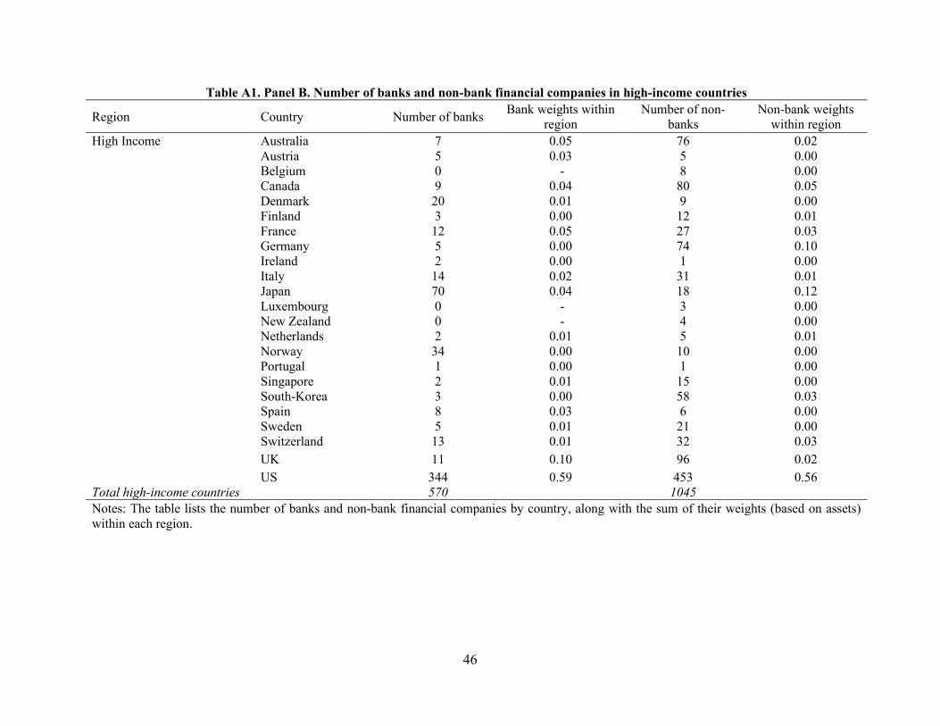
Table A1. Panel B. Number of banks and non-bank financial companies in high-income countries

Region Country Number of banks Bank weights within region

Number of non-banks

Non-bank weights within region

High Income Australia 7 0.05 76 0.02 Austria 5 0.03 5 0.00

Belgium 0 - 8 0.00 Canada 9 0.04 80 0.05 Denmark 20 0.01 9 0.00 Finland 3 0.00 12 0.01 France 12 0.05 27 0.03 Germany 5 0.00 74 0.10 Ireland 2 0.00 1 0.00 Italy 14 0.02 31 0.01 Japan 70 0.04 18 0.12 Luxembourg 0 - 3 0.00 New Zealand 0 - 4 0.00 Netherlands 2 0.01 5 0.01 Norway 34 0.00 10 0.00 Portugal 1 0.00 1 0.00 Singapore 2 0.01 15 0.00 South-Korea 3 0.00 58 0.03 Spain 8 0.03 6 0.00 Sweden 5 0.01 21 0.00 Switzerland 13 0.01 32 0.03 UK 11 0.10 96 0.02 US 344 0.59 453 0.56 Total high-income countries 570 1045 Notes: The table lists the number of banks and non-bank financial companies by country, along with the sum of their weights (based on assets) within each region.

47

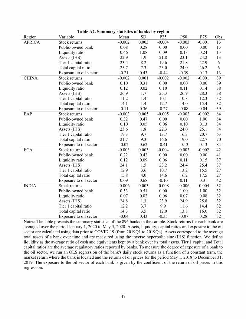
Table A2. Summary statistics of banks by region Region Variable Mean SD P25 P50 P75 Obs AFRICA Stock returns -0.002 0.003 -0.004 -0.003 -0.001 13 Public-owned bank 0.08 0.28 0.00 0.00 0.00 13 Liquidity ratio 0.46 1.08 0.09 0.18 0.24 13 Assets (IHS) 22.9 1.9 21.8 23.1 24.2 13 Tier 1 capital ratio 23.4 8.2 19.6 21.8 22.9 6 Total capital ratio 25.7 7.3 23.0 24.0 26.2 6 Exposure to oil sector -0.21 0.43 -0.44 -0.39 0.13 13 CHINA Stock returns -0.002 0.001 -0.002 -0.002 -0.001 39 Public-owned bank 0.10 0.31 0.00 0.00 0.00 39 Liquidity ratio 0.12 0.02 0.10 0.11 0.14 38 Assets (IHS) 26.9 1.7 25.3 26.9 28.3 38 Tier 1 capital ratio 11.2 1.4 10.1 10.8 12.3 32 Total capital ratio 14.1 1.4 12.7 14.0 15.4 32 Exposure to oil sector -0.11 0.36 -0.27 -0.08 0.04 39 EAP Stock returns -0.003 0.005 -0.005 -0.003 -0.002 84 Public-owned bank 0.32 0.47 0.00 0.00 1.00 84 Liquidity ratio 0.10 0.05 0.06 0.10 0.13 84 Assets (IHS) 23.6 1.8 22.3 24.0 25.1 84 Tier 1 capital ratio 19.3 9.7 13.7 16.3 20.7 63 Total capital ratio 21.7 9.3 16.6 19.0 22.7 70 Exposure to oil sector -0.02 0.62 -0.41 -0.13 0.13 84 ECA Stock returns -0.003 0.003 -0.004 -0.003 -0.002 42 Public-owned bank 0.22 0.42 0.00 0.00 0.00 41 Liquidity ratio 0.12 0.09 0.06 0.11 0.15 37 Assets (IHS) 24.1 1.5 23.2 24.4 25.4 37 Tier 1 capital ratio 12.9 3.6 10.7 13.2 15.5 27 Total capital ratio 15.8 4.0 14.6 16.2 17.5 27 Exposure to oil sector 0.09 0.68 -0.10 0.11 0.31 42 INDIA Stock returns -0.006 0.003 -0.008 -0.006 -0.004 32 Public-owned bank 0.53 0.51 0.00 1.00 1.00 32 Liquidity ratio 0.07 0.02 0.06 0.07 0.08 32 Assets (IHS) 24.8 1.3 23.9 24.9 25.8 32 Tier 1 capital ratio 12.2 3.7 9.9 11.6 14.4 32 Total capital ratio 14.3 3.5 12.0 13.8 16.0 32 Exposure to oil sector -0.04 0.43 -0.35 -0.07 0.28 32 Notes: The table presents the summary statistics of the 896 banks in the sample. Stock returns for each bank are averaged over the period January 1, 2020 to May 5, 2020. Assets, liquidity, capital ratios and exposure to the oil sector are calculated using data prior to COVID-19 (from 2019Q1 to 2019Q4). Assets correspond to the average total assets of a bank over time and are measured using the inverse hyperbolic sine (IHS) function. We define liquidity as the average ratio of cash and equivalents kept by a bank over its total assets. Tier 1 capital and Total capital ratios are the average regulatory ratios reported by banks. To measure the degree of exposure of a bank to the oil sector, we run an OLS regression of the bank's daily stock returns as a function of a constant term, the market return where the bank is located and the returns of oil prices for the period May 1, 2018 to December 31, 2019. The exposure to the oil sector of each bank is given by the coefficient of the return of oil prices in this regression.

48

Table A2. (Cont’d) Summary statistics of banks by region Region Variable Mean SD P25 P50 P75 Obs LAC Stock returns -0.004 0.003 -0.006 -0.004 -0.002 32 Public-owned bank 0.08 0.28 0.00 0.00 0.00 24 Liquidity ratio 0.28 0.81 0.05 0.11 0.17 24 Assets (IHS) 24.4 1.3 23.4 24.3 25.4 24 Tier 1 capital ratio 13.4 3.3 10.4 12.8 16.0 14 Total capital ratio 15.4 2.9 13.1 14.3 16.0 17 Exposure to oil sector 0.15 0.48 -0.14 0.26 0.46 32 MENA Stock returns -0.002 0.002 -0.004 -0.003 -0.001 84 Public-owned bank 0.36 0.48 0.00 0.00 1.00 84 Liquidity ratio 0.15 0.45 0.07 0.09 0.13 79 Assets (IHS) 24.1 1.4 23.0 24.1 25.2 79 Tier 1 capital ratio 15.0 3.5 11.9 15.5 17.8 61 Total capital ratio 17.1 3.0 14.7 17.3 18.8 61 Exposure to oil sector 0.03 0.58 -0.15 0.11 0.24 84 High-Income Stock returns -0.004 0.003 -0.006 -0.004 -0.002 570 Public-owned bank 0.02 0.15 0.00 0.00 0.00 563 Liquidity ratio 0.13 0.51 0.01 0.03 0.09 448 Assets (IHS) 23.8 2.4 21.8 23.3 25.0 460 Tier 1 capital ratio 14.2 5.2 12.0 13.2 15.3 348 Total capital ratio 15.1 5.6 12.7 14.2 16.5 406 Exposure to oil sector 0.10 1.49 -0.18 0.03 0.22 568 Notes: The table presents the summary statistics of the 896 banks in the sample. Stock returns for each bank are averaged over the period January 1, 2020 to May 5, 2020. Assets, liquidity, capital ratios and exposure to the oil sector are calculated using data prior to COVID-19 (from 2019Q1 to 2019Q4). Assets correspond to the average total assets of a bank over time and are measured using the inverse hyperbolic sine (IHS) function. We define liquidity as the average ratio of cash and equivalents kept by a bank over its total assets. Tier 1 capital and Total capital ratios are the average regulatory ratios reported by banks. To measure the degree of exposure of a bank to the oil sector, we run an OLS regression of the bank's daily stock returns as a function of a constant term, the market return where the bank is located and the returns of oil prices for the period May 1, 2018 to December 31, 2019. The exposure to the oil sector of each bank is given by the coefficient of the return of oil prices in this regression.

49

Table A3. Risk factors during the COVID-19 crisis (dependent variable: bank excess returns) January February March April (1) (2) (3) (4) (5) (6) (7) (8) (9) (10) (11) (12) Liquidity risk -0.745 -0.745 -0.650 -0.128 -0.103 -0.380 -3.030*** -3.027*** -3.949*** -0.483 -0.453 -0.526 [0.646] [0.652] [0.586] [0.494] [0.504] [0.364] [1.022] [1.018] [1.166] [0.474] [0.473] [0.422] Oil exposure 0.404** 0.404** 0.202 0.124 0.136 0.055 -1.986** -1.984** -2.366*** -0.299 -0.285 0.090 [0.200] [0.200] [0.167] [0.410] [0.415] [0.419] [0.755] [0.749] [0.576] [0.451] [0.453] [0.629] Size -0.380 -0.379 -0.817** -1.075*** -0.994*** -1.632** -2.039** -2.028*** -2.373** 1.091 1.184 2.069 [0.250] [0.259] [0.333] [0.292] [0.335] [0.662] [0.800] [0.752] [0.992] [0.717] [0.713] [1.326] Public banks -0.003 0.488 -1.515 -0.906 -0.203 0.392 -1.729 -2.138 [1.185] [1.216] [2.084] [2.220] [2.849] [2.986] [1.421] [1.424] Total capital 0.976** 1.318*** -1.576 0.093 [0.469] [0.388] [1.516] [0.286] Constant -1.857*** -1.857*** -2.371*** 0.467 0.600 -0.005 -5.475*** -5.457*** -5.809*** -4.905*** -4.753*** -4.576*** [0.581] [0.612] [0.616] [0.504] [0.553] [0.460] [1.551] [1.611] [1.638] [0.474] [0.488] [0.408] Observations 742 742 644 743 743 644 743 743 644 743 743 644 R-squared 0.130 0.130 0.162 0.107 0.110 0.187 0.177 0.177 0.220 0.038 0.040 0.057 Fixed Effects Region Region Region Region Region Region Region Region Region Region Region Region Cluster Country Country Country Country Country Country Country Country Country Country Country Country Notes: Cross sectional regressions of monthly excess returns. Excess returns are calculated as the bank stock returns during the month minus the returns of the domestic stock market index. All specifications include region fixed effects. Standard errors are clustered at the country level.

50

Table A4. Risk factors during the COVID-19 crisis (abnormal returns in dollars relative to global market index) January February March April (1) (2) (3) (4) (5) (6) (7) (8) (9) (10) (11) (12) Liquidity risk -0.486 -0.479 -0.361 0.408 0.440 0.187 -2.105* -2.089* -3.296*** 0.120 0.136 0.325 [0.613] [0.617] [0.569] [0.556] [0.565] [0.710] [1.188] [1.177] [1.161] [0.600] [0.601] [0.508] Oil exposure 0.770** 0.774** 0.602 0.708 0.723 0.904* -1.094 -1.087 -0.880 -0.322 -0.315 -0.220 [0.337] [0.339] [0.419] [0.516] [0.519] [0.501] [1.089] [1.090] [0.784] [0.469] [0.471] [0.498] Size -0.238 -0.214 -0.553 0.233 0.340 0.481 0.128 0.181 0.985 -0.858 -0.805 -1.245 [0.341] [0.335] [0.405] [0.326] [0.321] [0.383] [0.971] [0.962] [1.632] [0.715] [0.744] [0.799] Public banks -0.424 -0.006 -1.907 -1.802 -0.946 -1.845 -0.954 0.161 [1.317] [1.361] [2.183] [2.259] [2.405] [2.511] [1.313] [1.160] Total capital 0.530 1.307* -2.493 -0.157 [0.435] [0.766] [1.562] [0.404] Constant -0.553 -0.515 -1.032* -1.023 -0.854 -0.983 -8.098*** -8.014*** -7.161*** -2.642*** -2.557*** -3.249*** [0.534] [0.560] [0.563] [0.663] [0.698] [0.708] [1.754] [1.820] [1.558] [0.459] [0.506] [0.382] Observations 737 737 643 738 738 643 738 738 643 738 738 643 R-squared 0.172 0.172 0.207 0.189 0.193 0.240 0.245 0.245 0.319 0.132 0.132 0.165 Fixed Effects Region Region Region Region Region Region Region Region Region Region Region Region Cluster Country Country Country Country Country Country Country Country Country Country Country Country Notes: Cross sectional regressions of monthly abnormal returns. Abnormal returns are calculated in dollars as the difference between realized returns and the expected returns implied by a market model based on a global market index. All specifications include region fixed effects. Standard errors are clustered at the country level.

51

Table A5. Risk factors during the COVID-19 crisis (based on Fama–French three-factor model) January February March April (1) (2) (3) (4) (5) (6) (7) (8) (9) (10) (11) (12) Liquidity risk -0.678 -0.687 -0.233 0.114 0.130 0.040 -2.471 -2.495 -3.974*** 0.154 0.171 0.345 [0.750] [0.748] [0.687] [0.849] [0.855] [0.791] [1.645] [1.644] [1.221] [0.617] [0.619] [0.501] Oil exposure 0.747 0.743 0.480 0.557 0.564 0.838 -2.046 -2.057* -1.349 -0.199 -0.191 -0.313 [0.561] [0.563] [0.654] [0.683] [0.686] [0.696] [1.226] [1.224] [0.976] [0.597] [0.596] [0.630] Size 0.866 0.839 1.215** 0.413 0.465 0.917** 1.276 1.199 3.290* 0.213 0.268 0.026 [0.586] [0.595] [0.508] [0.491] [0.502] [0.434] [1.147] [1.133] [1.923] [0.639] [0.649] [0.861] Public banks 0.493 0.579 -0.934 -0.913 1.381 0.163 -0.991 -0.217 [1.285] [1.361] [1.789] [1.789] [3.753] [4.049] [1.413] [1.230] Total capital 0.953 1.538* -1.953 0.217 [0.617] [0.805] [1.367] [0.429] Constant 1.725** 1.682** 1.495** 0.155 0.238 0.143 -1.871 -1.993 -0.271 -4.048*** -3.960*** -4.505*** [0.666] [0.704] [0.628] [0.737] [0.767] [0.729] [1.904] [2.014] [1.490] [0.510] [0.562] [0.401] Observations 737 737 643 738 738 643 738 738 643 738 738 643 R-squared 0.166 0.166 0.172 0.145 0.145 0.161 0.202 0.202 0.273 0.085 0.086 0.110 Fixed Effects Region Region Region Region Region Region Region Region Region Region Region Region Cluster Country Country Country Country Country Country Country Country Country Country Country Country Notes: Cross sectional regressions of monthly abnormal returns. Abnormal returns are the difference between realized returns and the expected returns implied by the Fama–French three-factor model. All specifications include region fixed effects. Standard errors are clustered at the country level.

52

Table A6. Policy announcements in developed and developing countries Developed Countries Developing Countries (days with policy announcements = 160) (days with policy announcements = 115)

Announcements by

category Single policy

announcements Announcements by

category Single policy

announcements Policy category Liquidity 40 14 43 18 Prudential 99 47 42 18 Borrower Support 57 11 32 16 Asset Purchases 22 17 8 2 Policy Rates 10 6 36 28 Total policies 228 95 161 82 Policy categories announced in the same day Liquidity + Prudential 13 7 Liquidity + Borrower Support 9 2 Liquidity + Prudential + Borrower Support 1 5 Liquidity + Policy Rates 2 3 Liquidity + Asset Purchases 0 3 Prudential + Borrower Support 35 6 Prudential + Policy Rates 0 2 Prudential + Liquidity + Asset Purchases 1 1 Borrower Support + Liquidity + Policy Rates 0 1 Borrower Support + Asset Purchases + Policy Rates 1 0 Policy Rates + Asset Purchases 1 0 Policy Rates + Liquidity + Prudential 0 1 Asset Purchases + Prudential 2 0 Notes: Data obtained from the World Bank (World Bank, 2020) covering the period February 1 to April 17 2020.

53

Table A7. Impact of unexpected monetary policy rate announcements (1) (2) (3) (4) n = 0 3 0 3 Liquidity risk 0.284 1.502* 0.203 1.348 (0.415) (0.887) (0.477) (1.505) Oil exposure -0.752* -1.741** -0.859** -1.983** (0.388) (0.802) (0.273) (0.820) Size 0.474 1.055 0.299 0.675 (0.394) (0.810) (0.434) (0.768) Public banks 1.095 2.401 (0.982) (1.443) Constant 0.542* -0.691 0.322 -1.168*** (0.323) (0.666) (0.339) (0.214) Observations 87 86 87 86 R-squared 0.266 0.395 0.283 0.412 Notes: The table presents the estimates of cross-sectional regressions of the impact of financial sector policies on the excess returns of banks on announcement days (n=0) and three days after the announcement (n=3). Excess returns are calculated as the bank stock returns during the month minus the returns of the domestic stock market index. All specifications include region fixed effects. Standard errors are clustered at the country level.