Barrier Optionsa - 國立臺灣大學lyuu/finance1/2012/20120321.pdf · Barrier Optionsa • Their...

Barrier Optionsa

• Their payoff depends on whether the underlying asset’s

price reaches a certain price level H.

• A knock-out option is an ordinary European option

which ceases to exist if the barrier H is reached by the

price of its underlying asset.

• A call knock-out option is sometimes called a

down-and-out option if H < S.

• A put knock-out option is sometimes called an

up-and-out option when H > S.aA former MBA student in finance told me on March 26, 2004, that

she did not understand why I covered barrier options until she started

working in a bank. She was working for Lehman Brothers in HK as of

April, 2006.

c⃝2012 Prof. Yuh-Dauh Lyuu, National Taiwan University Page 323

H

Time

Price

S Barrier hit


Barrier Options (concluded)

• A knock-in option comes into existence if a certain

barrier is reached.

• A down-and-in option is a call knock-in option that

comes into existence only when the barrier is reached

and H < S.

• An up-and-in is a put knock-in option that comes into

existence only when the barrier is reached and H > S.

• Formulas exist for all the possible barrier options

mentioned above.a

aHaug (1998).


A Formula for Down-and-In Callsa

• Assume X ≥ H.

• The value of a European down-and-in call on a stockpaying a dividend yield of q is

Se−qτ

(H

S

)2λ

N(x)−Xe−rτ

(H

S

)2λ−2

N(x− σ√τ),

(28)

– x ≡ ln(H2/(SX))+(r−q+σ2/2) τσ√τ

.

– λ ≡ (r − q + σ2/2)/σ2.

• A European down-and-out call can be priced via the

in-out parity (see text).

aMerton (1973).


A Formula for Up-and-In Putsa

• Assume X ≤ H.

• The value of a European up-and-in put is

Xe−rτ

(H

S

)2λ−2

N(−x+ σ√τ)− Se−qτ

(H

S

)2λ

N(−x).

• Again, a European up-and-out put can be priced via the

in-out parity.

aMerton (1973).


Are American Options Barrier Options?a

• American options are barrier options with the exercise

boundary as the barrier and the payoff as the rebate?

• One salient difference is that the exercise boundary must

be derived during backward induction.

• But the barrier in a barrier option is given a priori.

aContributed by Mr. Yang, Jui-Chung (D97723002) on March 25,

2009.


Interesting Observations

• Assume H < X.

• Replace S in the pricing formula for the down-and-in

call, Eq. (28) on p. 326, with H2/S.

• Equation (28) becomes Eq. (26) on p. 278 when

r − q = σ2/2.

• Equation (28) becomes S/H times Eq. (26) on p. 278

when r − q = 0.

• Why?


Binomial Tree Algorithms

• Barrier options can be priced by binomial tree

algorithms.

• Below is for the down-and-out option.

0 H


H

8

16

4

32

8

2

64

16

4

1

4.992

12.48

1.6

27.2

4.0

0

58

10

0

0

X

0.0

S = 8, X = 6, H = 4, R = 1.25, u = 2, and d = 0.5.

Backward-induction: C = (0.5× Cu + 0.5× Cd)/1.25.


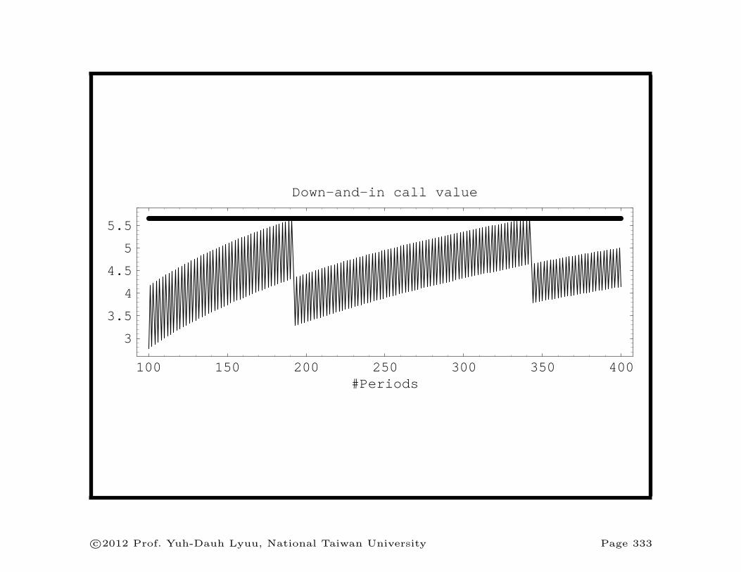
Binomial Tree Algorithms (concluded)

• But convergence is erratic because H is not at a price

level on the tree (see plot on next page).

– The barrier has to be adjusted to be at a price level.

– The “effective barrier” changes as n increases.

• In fact, the binomial tree is O(1/√n) convergent.a

• Solutions will be presented later.

aLin (R95221010) (2008).


100 150 200 250 300 350 400#Periods

3

3.5

4

4.5

5

5.5

Down-and-in call value


Daily Monitoring

• Almost all barrier options monitor the barrier only for

daily closing prices.

• If so, only nodes at the end of a day need to check for

the barrier condition.

• We can even remove intraday nodes to create a

multinomial tree.

– A node is then followed by d+ 1 nodes if each day is

partitioned into d periods.

• Does this save time or space?a

aContributed by Ms. Chen, Tzu-Chun (R94922003) and others on

April 12, 2006.


A Heptanomial Tree (6 Periods Per Day)

-� 1 day


Foreign Currencies

• S denotes the spot exchange rate in domestic/foreign

terms.a

• σ denotes the volatility of the exchange rate.

• r denotes the domestic interest rate.

• r̂ denotes the foreign interest rate.

• A foreign currency is analogous to a stock paying a

known dividend yield.

– Foreign currencies pay a “continuous dividend yield”

equal to r̂ in the foreign currency.

aBy that we mean the number of domestic currencies per unit of

foreign currency. The market convention is the opposite.


Foreign Exchange Options

• Foreign exchange options are settled via delivery of the

underlying currency.

• A primary use of foreign exchange (or forex) options is

to hedge currency risk.

• Consider a U.S. company expecting to receive 100

million Japanese yen in March 2000.

• Those 100 million Japanese yen will be exchanged for

U.S. dollars.


Foreign Exchange Options (continued)

• The contract size for the Japanese yen option is

JPY6,250,000.

• The company purchases 100,000,000/6,250,000 = 16

puts on the Japanese yen with a strike price of $.0088

and an exercise month in March 2000.

• This gives the company the right to sell 100,000,000

Japanese yen for 100,000,000× .0088 = 880,000 U.S.

dollars.


Foreign Exchange Options (concluded)

• The formulas derived for stock index options in Eqs. (26)

on p. 278 apply with the dividend yield equal to r̂:

C = Se−r̂τN(x)−Xe−rτN(x− σ√τ), (29)

P = Xe−rτN(−x+ σ√τ)− Se−r̂τN(−x).

(29′)

– Above,

x ≡ ln(S/X) + (r − r̂ + σ2/2) τ

σ√τ

.


Bar the roads!

Bar the paths!

Wert thou to flee from here, wert thou

to find all the roads of the world,

the way thou seekst

the path to that thou’dst find not[.]

— Richard Wagner (1813–1883), Parsifal


Path-Dependent Derivatives

• Let S0, S1, . . . , Sn denote the prices of the underlying

asset over the life of the option.

• S0 is the known price at time zero.

• Sn is the price at expiration.

• The standard European call has a terminal value

depending only on the last price, max(Sn −X, 0).

• Its value thus depends only on the underlying asset’s

terminal price regardless of how it gets there.


Path-Dependent Derivatives (continued)

• Some derivatives are path-dependent in that their

terminal payoff depends critically on the path.

• The (arithmetic) average-rate call has this terminal

value:

max

(1

n+ 1

n∑i=0

Si −X, 0

).

• The average-rate put’s terminal value is given by

max

(X − 1

n+ 1

n∑i=0

Si, 0

).


Path-Dependent Derivatives (continued)

• Average-rate options are also called Asian options.

• They are very popular.a

• They are useful hedging tools for firms that will make a

stream of purchases over a time period because the costs

are likely to be linked to the average price.

• They are mostly European.

aAs of the late 1990s, the outstanding volume was in the range of

5–10 billion U.S. dollars according to Nielsen and Sandmann (2003).


Path-Dependent Derivatives (concluded)

• A lookback call option on the minimum has a terminal

payoff of Sn −min0≤i≤n Si.

• A lookback put on the maximum has a terminal payoff

of max0≤i≤n Si − Sn.

• The fixed-strike lookback option provides a payoff of

– max(max0≤i≤n Si −X, 0) for the call.

– max(X −min0≤i≤n Si, 0) for the put.

• Lookback calls and puts on the average (instead of a

constant X) are called average-strike options.


Average-Rate Options

• Average-rate options are notoriously hard to price.

• The binomial tree for the averages does not combine (see

next page).

• A naive algorithm enumerates the 2n price paths for an

n-period binomial tree and then averages the payoffs.

• But the complexity is exponential.

• As a result, the Monte Carlo method and approximation

algorithms are some of the alternatives left.


S

Su

Sd

Suu

Sud

Sdu

Sdd

p

1− p

−++= ��PD[ ;6XX6X6&XX

−++= ��PD[ ;6XG6X6&XG

−++= ��PD[ ;6GX6G6&GX

−++= ��PD[ ;6GG6G6&GG

( )U

XGXXX H

&SS&& −+= �

( )U

GGGXG H

&SS&& −+= �

( )U

GXH

&SS&& −+= �

p

1− p

p

1− p

p

1− p

p

1− p

p

1− p


States and Their Transitions

• The tuple

(i, S, P )

captures the statea for the Asian option.

– i: the time.

– S: the prevailing stock price.

– P : the running sum.b

aA “sufficient statistic,” if you will.bWhat if the average is a moving average?


States and Their Transitions (concluded)

• For the binomial model, the state transition is:

(i+ 1, Su, P + Su), for the up move

↗(i, S, P )

↘(i+ 1, Sd, P + Sd), for the down move


Pricing Some Path-Dependent Options

• Not all path-dependent derivatives are hard to price.

• Barrier options are easy to price.

• When averaging is done geometrically, the option payoffs

are

max((S0S1 · · ·Sn)

1/(n+1) −X, 0),

max(X − (S0S1 · · ·Sn)

1/(n+1), 0).


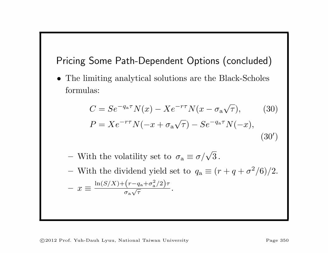
Pricing Some Path-Dependent Options (concluded)

• The limiting analytical solutions are the Black-Scholes

formulas:

C = Se−qaτN(x)−Xe−rτN(x− σa

√τ), (30)

P = Xe−rτN(−x+ σa

√τ)− Se−qaτN(−x),

(30′)

– With the volatility set to σa ≡ σ/√3 .

– With the dividend yield set to qa ≡ (r + q + σ2/6)/2.

– x ≡ ln(S/X)+(r−qa+σ2a/2)τ

σa√τ

.


An Approximate Formula for Asian Callsa

C = e−rτ

[S

τ

∫ τ

0

eµt+σ2t/2N

(−γ + (σt/τ)(τ − t/2)√

τ/3

)dt

−XN

(−γ√τ/3

)],

where

• µ ≡ r − σ2/2.

• γ is the unique value that satisfies

S

τ

∫ τ

0

e3γσt(τ−t/2)/τ2+µt+σ2[ t−(3t2/τ3)(τ−t/2)2 ]/2 dt = X.

aRogers and Shi (1995); Thompson (1999); Chen (R92723061) (2005);

Chen (R92723061) and Lyuu (2006).


Approximation Algorithm for Asian Options

• Based on the BOPM.

• Consider a node at time j with the underlying asset

price equal to S0uj−idi.

• Name such a node N(j, i).

• The running sum∑j

m=0 Sm at this node has a

maximum value of

S0(1 +

j︷︸︸︷u+ u2 + · · ·+ uj−i + uj−id+ · · ·+ uj−idi)

= S01− uj−i+1

1− u+ S0u

j−id1− di

1− d.


Path with maximum running average

Path with minimum running average

N


Approximation Algorithm for Asian Options(continued)

• Divide this value by j + 1 and call it Amax(j, i).

• Similarly, the running sum has a minimum value of

S0(1 +

j︷︸︸︷d+ d2 + · · ·+ di + diu+ · · ·+ diuj−i)

= S01− di+1

1− d+ S0d

iu1− uj−i

1− u.

• Divide this value by j + 1 and call it Amin(j, i).

• Amin and Amax are running averages.



• The possible running averages at N(j, i) are far too

many:(ji

).

– For example,(

jj/2

)≈ 2j

√2/(πj) .

• But all must lie between Amin(j, i) and Amax(j, i).

• Pick k + 1 equally spaced values in this range and treat

them as the true and only running averages:

Am(j, i) ≡(k −m

k

)Amin(j, i) +

(mk

)Amax(j, i)

for m = 0, 1, . . . , k.


m

A min ( j , i )

A max ( j , i )

A m ( j , i )



• Such “bucketing” introduces errors, but it works

reasonably well in practice.a

• A better alternative picks values whose logarithms are

equally spaced.

• Still other alternatives are possible.

• Generally, k must scale with at least n to show

convergence.b

aHull and White (1993).bDai (R86526008, D8852600), Huang (F83506075), and Lyuu (2002).



• Backward induction calculates the option values at each

node for the k + 1 running averages.

• Suppose the current node is N(j, i) and the running

average is a.

• Assume the next node is N(j + 1, i), after an up move.

• As the asset price there is S0uj+1−idi, we seek the

option value corresponding to the new running average

Au ≡ (j + 1) a+ S0uj+1−idi

j + 2.



• But Au is not likely to be one of the k + 1 running

averages at N(j + 1, i)!

• Find the 2 running averages that bracket it:

Aℓ(j + 1, i) ≤ Au ≤ Aℓ+1(j + 1, i).

• Express Au as a linearly interpolated value of the two

running averages,

Au = xAℓ(j + 1, i) + (1− x)Aℓ+1(j + 1, i), 0 ≤ x ≤ 1.


0 ...m ...k

�

0...ℓℓ+ 1...k

0...ℓ′

ℓ′ + 1...k



• Obtain the approximate option value given the running

average Au via

Cu ≡ xCℓ(j + 1, i) + (1− x)Cℓ+1(j + 1, i).

– Cℓ(t, s) denotes the option value at node N(t, s)

with running average Aℓ(t, s).

• This interpolation introduces the second source of error.



• The same steps are repeated for the down node

N(j + 1, i+ 1) to obtain another approximate option

value Cd.

• Finally obtain the option value as

[ pCu + (1− p)Cd ] e−r∆t.

• The running time is O(kn2).

– There are O(n2) nodes.

– Each node has O(k) buckets.


Approximation Algorithm for Asian Options(concluded)

• Arithmetic average-rate options were assumed to be

newly issued: no historical average to deal with.

• This problem can be easily addressed (see text).

• How about the Greeks?a

aThanks to a lively class discussion on March 31, 2004.


A Numerical Example

• Consider a European arithmetic average-rate call with

strike price 50.

• Assume zero interest rate in order to dispense with

discounting.

• The minimum running average at node A in the figure

on p. 365 is 48.925.

• The maximum running average at node A in the same

figure is 51.149.


51.1

68

49.500 50

.612

51.7

23

48.944

53.506

48.979

50.05

6 48.388

46.827

52.356

50

53.447

46.775

0.0269

50.056

51.206

47.903

50.056

0.2956

0.5782

0.8617

50.056

1.206

0.056

2.356

3.506

49.666

48.925

50.408

51.149

0.000

0.000

0.000

0.056 p = 0.483

u = 1.069 d = 0.936

A

B

C


A Numerical Example (continued)

• Each node picks k = 3 for 4 equally spaced running

averages.

• The same calculations are done for node A’s successor

nodes B and C.

• Suppose node A is 2 periods from the root node.

• Consider the up move from node A with running

average 49.666.



• Because the stock price at node B is 53.447, the new

running average will be

3× 49.666 + 53.447

4≈ 50.612.

• With 50.612 lying between 50.056 and 51.206 at node B,

we solve

50.612 = x× 50.056 + (1− x)× 51.206

to obtain x ≈ 0.517.



• The option value corresponding to running average

50.056 at node B is 0.056.

• The option values corresponding to running average

51.206 at node B is 1.206.

• Their contribution to the option value corresponding to

running average 49.666 at node A is weighted linearly as

x× 0.056 + (1− x)× 1.206 ≈ 0.611.



• Now consider the down move from node A with running

average 49.666.

• Because the stock price at node C is 46.775, the new

running average will be

3× 49.666 + 46.775

4≈ 48.944.

• With 48.944 lying between 47.903 and 48.979 at node C,

we solve

48.944 = x× 47.903 + (1− x)× 48.979

to obtain x ≈ 0.033.


A Numerical Example (concluded)

• The option values corresponding to running averages

47.903 and 48.979 at node C are both 0.0.

• Their contribution to the option value corresponding to

running average 49.666 at node A is 0.0.

• Finally, the option value corresponding to running

average 49.666 at node A equals

p× 0.611 + (1− p)× 0.0 ≈ 0.2956,

where p = 0.483.

• The remaining three option values at node A can be

computed similarly.


Convergence Behavior of the ApproximationAlgorithma

60 80 100 120 140n

0.325

0.33

0.335

0.34

0.345

0.35

Asian option value

aDai (R86526008, D8852600) and Lyuu (2002).


Remarks on Asian Option Pricing

• Asian option pricing is an active research area.

• The above algorithm overestimates the “true” value.a

• To guarantee convergence, k needs to grow with n.

• There is a convergent approximation algorithm that

does away with interpolation with a provable running

time of 2O(√n ).b

aDai (R86526008, D8852600), Huang (F83506075), and Lyuu (2002).bDai (R86526008, D8852600) and Lyuu (2002, 2004).


Remarks on Asian Option Pricing (continued)

• There is an O(kn2)-time algorithm with an error bound

of O(Xn/k) from the naive O(2n)-time binomial tree

algorithm in the case of European Asian options.a

– k can be varied for trade-off between time and

accuracy.

– If we pick k = O(n2), then the error is O(1/n), and

the running time is O(n4).

• In practice, log-linear interpolation works better.

aAingworth, Motwani, and Oldham (2000).


Remarks on Asian Option Pricing (continued)

• Another approximation algorithm reduces the error to

O(X√n/k).a

– It varies the number of buckets per node.

– If we pick k = O(n), the error is O(n−0.5).

– If we pick k = O(n1.5), then the error is O(1/n), and

the running time is O(n3.5).

• Under “reasonable assumptions,” an O(n2)-time

algorithm with an error bound of O(1/n) exists.b

aDai (R86526008, D8852600), Huang (F83506075), and Lyuu (2002).bHsu (R7526001) and Lyuu (2004).


Remarks on Asian Option Pricing (concluded)

• The basic idea is a nonuniform allocation of running

averages instead of a uniform k.

• It strikes a balance between error and complexity.

Uniform allocation

05

10

15

20

i j

0

20

40

k

05

10

15

20

i

Nonuniform allocation

05

10

15

20

i j

0

100

200

300

400

kij

05

10

15

20

i


A Grand Comparisona

aHsu (R7526001) and Lyuu (2004); Zhang (2001,2003); Chen

(R92723061) and Lyuu (2006).


X σ r Exact AA2 AA3 Hsu-Lyuu Chen-Lyuu

95 0.05 0.05 7.1777275 7.1777244 7.1777279 7.178812 7.177726

100 2.7161745 2.7161755 2.7161744 2.715613 2.716168

105 0.3372614 0.3372601 0.3372614 0.338863 0.337231

95 0.09 8.8088392 8.8088441 8.8088397 8.808717 8.808839

100 4.3082350 4.3082253 4.3082331 4.309247 4.308231

105 0.9583841 0.9583838 0.9583841 0.960068 0.958331

95 0.15 11.0940944 11.0940964 11.0940943 11.093903 11.094094

100 6.7943550 6.7943510 6.7943553 6.795678 6.794354

105 2.7444531 2.7444538 2.7444531 2.743798 2.744406

90 0.10 0.05 11.9510927 11.9509331 11.9510871 11.951610 11.951076

100 3.6413864 3.6414032 3.6413875 3.642325 3.641344

110 0.3312030 0.3312563 0.3311968 0.331348 0.331074

90 0.09 13.3851974 13.3851165 13.3852048 13.385563 13.385190

100 4.9151167 4.9151388 4.9151177 4.914254 4.915075

110 0.6302713 0.6302538 0.6302717 0.629843 0.630064

90 0.15 15.3987687 15.3988062 15.3987860 15.398885 15.398767

100 7.0277081 7.0276544 7.0277022 7.027385 7.027678

110 1.4136149 1.4136013 1.4136161 1.414953 1.413286


A Grand Comparison (concluded)

X σ r Exact AA2 AA3 Hsu-Lyuu Chen-Lyuu

90 0.20 0.05 12.5959916 12.5957894 12.5959304 12.596052 12.595602

100 5.7630881 5.7631987 5.7631187 5.763664 5.762708

110 1.9898945 1.9894855 1.9899382 1.989962 1.989242

90 0.09 13.8314996 13.8307782 13.8313482 13.831604 13.831220

100 6.7773481 6.7775756 6.7773833 6.777748 6.776999

110 2.5462209 2.5459150 2.5462598 2.546397 2.545459

90 0.15 15.6417575 15.6401370 15.6414533 15.641911 15.641598

100 8.4088330 8.4091957 8.4088744 8.408966 8.408519

110 3.5556100 3.5554997 3.5556415 3.556094 3.554687

90 0.30 0.05 13.9538233 13.9555691 13.9540973 13.953937 13.952421

100 7.9456288 7.9459286 7.9458549 7.945918 7.944357

110 4.0717942 4.0702869 4.0720881 4.071945 4.070115

90 0.09 14.9839595 14.9854235 14.9841522 14.984037 14.982782

100 8.8287588 8.8294164 8.8289978 8.829033 8.827548

110 4.6967089 4.6956764 4.6969698 4.696895 4.694902

90 0.15 16.5129113 16.5133090 16.5128376 16.512963 16.512024

100 10.2098305 10.2110681 10.2101058 10.210039 10.208724

110 5.7301225 5.7296982 5.7303567 5.730357 5.728161


Forwards, Futures, Futures Options, Swaps


Summon the nations to come to the trial.

Which of their gods can predict the future?

— Isaiah 43:9

The sure fun of the evening

outweighed the uncertain treasure[.]

— Mark Twain (1835–1910),

The Adventures of Tom Sawyer


Terms

• r will denote the riskless interest rate.

• The current time is t.

• The maturity date is T .

• The remaining time to maturity is τ ≡ T − t (all

measured in years).

• The spot price S, the spot price at maturity is ST .

• The delivery price is X.


Terms (concluded)

• The forward or futures price is F for a newly written

contract.

• The value of the contract is f .

• A price with a subscript t usually refers to the price at

time t.

• Continuous compounding will be assumed.


Forward Contracts

• Forward contracts are for the delivery of the underlying

asset for a certain delivery price on a specific time.

– Foreign currencies, bonds, corn, etc.

• Ideal for hedging purposes.

• A farmer enters into a forward contract with a food

processor to deliver 100,000 bushels of corn for $2.5 per

bushel on September 27, 1995.

• The farmer is assured of a buyer at an acceptable price.

• The processor knows the cost of corn in advance.


Forward Contracts (concluded)

• A forward agreement limits both risk and rewards.

– If the spot price of corn rises on the delivery date,

the farmer will miss the opportunity of extra profits.

– If the price declines, the processor will be paying

more than it would.

• Either side has an incentive to default.

• Other problems: The food processor may go bankrupt,

the farmer can go bust, the farmer might not be able to

harvest 100,000 bushels of corn because of bad weather,

the cost of growing corn may skyrocket, etc.


Spot and Forward Exchange Rates

• Let S denote the spot exchange rate.

• Let F denote the forward exchange rate one year from

now (both in domestic/foreign terms).

• rf denotes the annual interest rate of the foreign

currency.

• rℓ denotes the annual interest rate of the local currency.

• Arbitrage opportunities will arise unless these four

numbers satisfy an equation.


Interest Rate Paritya

F

S= erℓ−rf . (31)

• A holder of the local currency can do either of:

– Lend the money in the domestic market to receive

erℓ one year from now.

– Convert local currency for foreign currency, lend for 1

year in foreign market, and convert foreign currency

into local currency at the fixed forward exchange

rate, F , by selling forward foreign currency now.

aKeynes (1923). John Maynard Keynes (1883–1946) was one of the

greatest economists in history.


Interest Rate Parity (concluded)

• No money changes hand in entering into a forward

contract.

• One unit of local currency will hence become Ferf/S

one year from now in the 2nd case.

• If Ferf/S > erℓ , an arbitrage profit can result from

borrowing money in the domestic market and lending it

in the foreign market.

• If Ferf/S < erℓ , an arbitrage profit can result from

borrowing money in the foreign market and lending it in

the domestic market.


Forward Price

• The payoff of a forward contract at maturity is

ST −X.

• Forward contracts do not involve any initial cash flow.

• The forward price is the delivery price which makes the

forward contract zero valued.

– That is, f = 0 when X = F .


Forward Price (concluded)

• The delivery price cannot change because it is written in

the contract.

• But the forward price may change after the contract

comes into existence.

– The value of a forward contract, f , is 0 at the outset.

– It will fluctuate with the spot price thereafter.

– This value is enhanced when the spot price climbs

and depressed when the spot price declines.

• The forward price also varies with the maturity of the

contract.


Forward Price: Underlying Pays No Income

Lemma 11 For a forward contract on an underlying asset

providing no income,

F = Serτ . (32)

• If F > Serτ :

– Borrow S dollars for τ years.

– Buy the underlying asset.

– Short the forward contract with delivery price F .


Proof (concluded)

• At maturity:

– Deliver the asset for F .

– Use Serτ to repay the loan, leaving an arbitrage

profit of F − Serτ > 0.

• If F < Serτ , do the opposite.


Example

• r is the annualized 3-month riskless interest rate.

• S is the spot price of the 6-month zero-coupon bond.

• A new 3-month forward contract on a 6-month

zero-coupon bond should command a delivery price of

Ser/4.

• So if r = 6% and S = 970.87, then the delivery price is

970.87× e0.06/4 = 985.54.


Contract Value: The Underlying Pays No Income

The value of a forward contract is

f = S −Xe−rτ .

• Consider a portfolio of one long forward contract, cash

amount Xe−rτ , and one short position in the underlying

asset.

• The cash will grow to X at maturity, which can be used

to take delivery of the forward contract.

• The delivered asset will then close out the short position.

• Since the value of the portfolio is zero at maturity, its

PV must be zero.


Forward Price: Underlying Pays Predictable Income

Lemma 12 For a forward contract on an underlying asset

providing a predictable income with a PV of I,

F = (S − I) erτ . (33)

• If F > (S − I) erτ , borrow S dollars for τ years, buy

the underlying asset, and short the forward contract

with delivery price F .

• At maturity, the asset is delivered for F , and

(S − I) erτ is used to repay the loan, leaving an

arbitrage profit of F − (S − I) erτ > 0.

• If F < (S − I) erτ , reverse the above.


Example

• Consider a 10-month forward contract on a $50 stock.

• The stock pays a dividend of $1 every 3 months.

• The forward price is(50− e−r3/4 − e−r6/2 − e−3×r9/4

)er10×(10/12).

– ri is the annualized i-month interest rate.


Underlying Pays a Continuous Dividend Yield of q

The value of a forward contract at any time prior to T is

f = Se−qτ −Xe−rτ . (34)


Futures Contracts vs. Forward Contracts

• They are traded on a central exchange.

• A clearinghouse.

– Credit risk is minimized.

• Futures contracts are standardized instruments.

• Gains and losses are marked to market daily.

– Adjusted at the end of each trading day based on the

settlement price.


Date post:	07-Sep-2019
Category:	Documents
Upload:	others
View:	2 times
Download:	0 times

Barrier Optionsa - 國立臺灣大學lyuu/finance1/2012/20120321.pdf · Barrier Optionsa • Their...

Documents