39
Weather Impact Modeling Based on Joe Mitchell’s slides
| Date post: | 02-Dec-2018 |
| Category: |
Documents |
| Upload: | trinhquynh |
| View: | 216 times |
| Download: | 0 times |

Weather Impact Modeling
Based on
Joe Mitchell’s slides

Weather Aviation
tailored to
aviation needs
ready for
integration
traffic manager
Forecast Products ATM Automation
Old Paradigm: Human Centric
New Paradigm: Automation Centric
Workshop 2: Weather Constraint Modeling
March 3-4, 2008
Matthias Steiner and Robert Sharman, NCARTranslation of Weather Information to TFM Impact
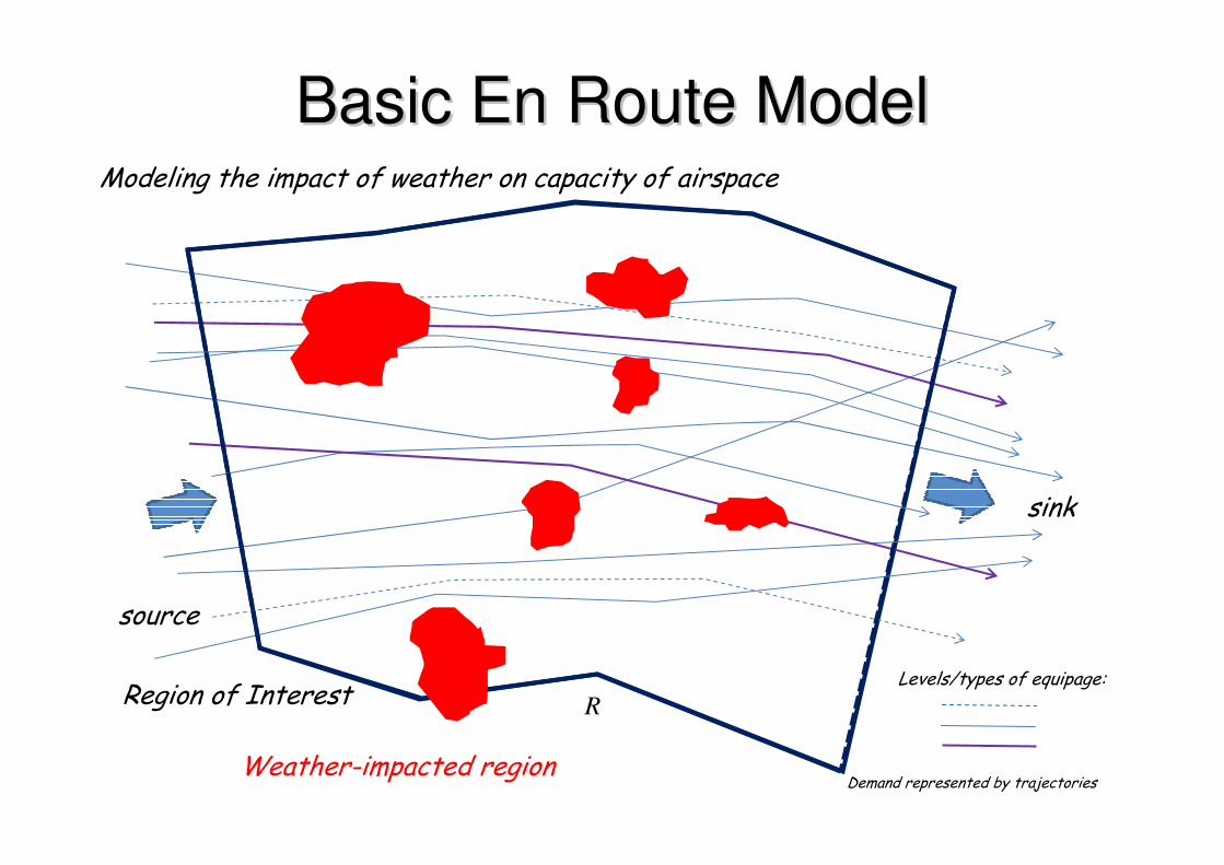
Basic En Route ModelBasic En Route Model
Region of Interest R
Levels/types of equipage:
source
sink
Demand represented by trajectoriesWeather-impacted region
Modeling the impact of weather on capacity of airspace

More General ModelMore General Model
4Weather-impacted region (Type 1) (Type 2) (Type 3)
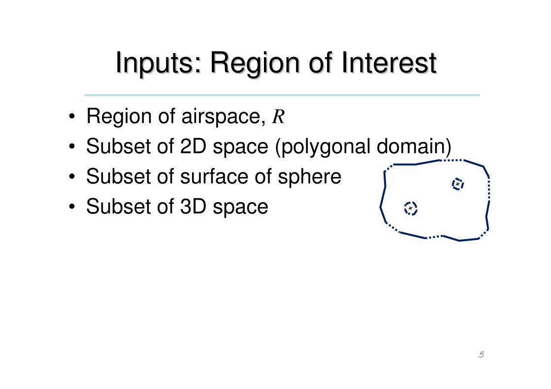
Inputs: Region of InterestInputs: Region of Interest
• Region of airspace, R
• Subset of 2D space (polygonal domain)
• Subset of surface of sphere
• Subset of 3D space
5

Inputs: Time HorizonInputs: Time Horizon
• Time window, [t1, t2], of interest
• Sliding time window [t1, t2]
• Updates every ∆t
6
10:15
t1 t2

Inputs: DemandInputs: Demand
• “Demand” given as a set of trajectories (flights) in space-time:
� τ : (x1,y1,z1,t1), (x2,y2,z2,t2), (x3,y3,z3,t3), …
• Each trajectory τ has associated with it
– Probability distribution of time Tτ when τ enters R
• Given by ETA estimator
– Equipage class, i, which includes information about the aircraft,
specifying a set Σi of preferences and parameters
– Priority, specified as an integer ∈ {1,2,…,NP}
– Entrance point (or window), where it enters R
– Exit point (or window) where it will leave R
7
More detail below
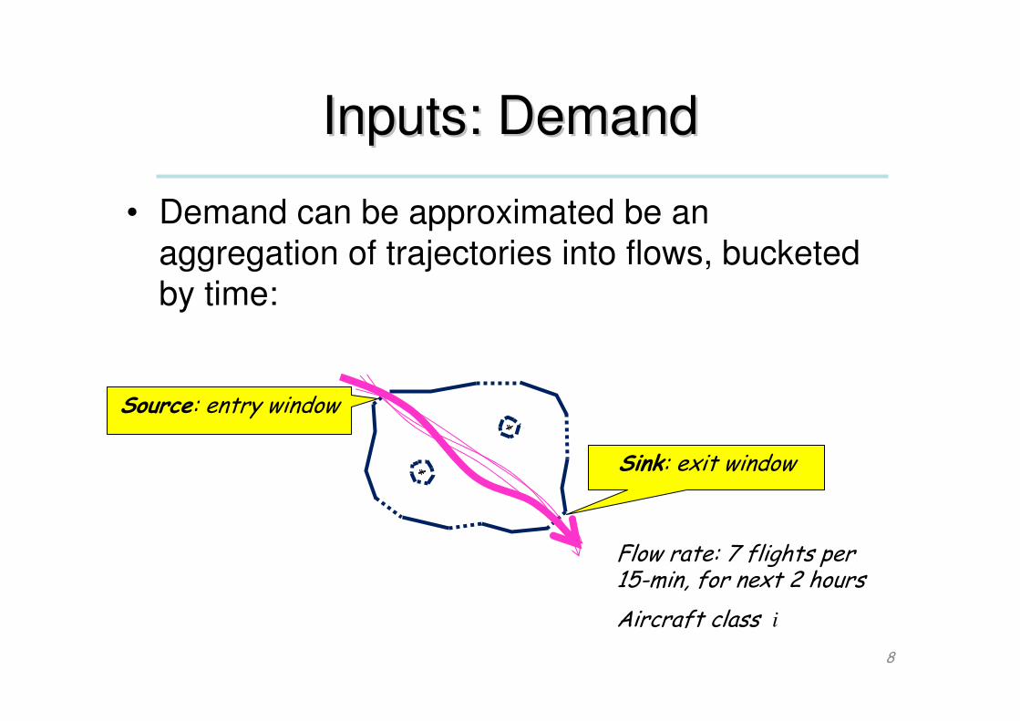
Inputs: DemandInputs: Demand
• Demand can be approximated be an
aggregation of trajectories into flows, bucketed
by time:
8
Flow rate: 7 flights per 15-min, for next 2 hours
Aircraft class i
Source: entry window
Sink: exit window
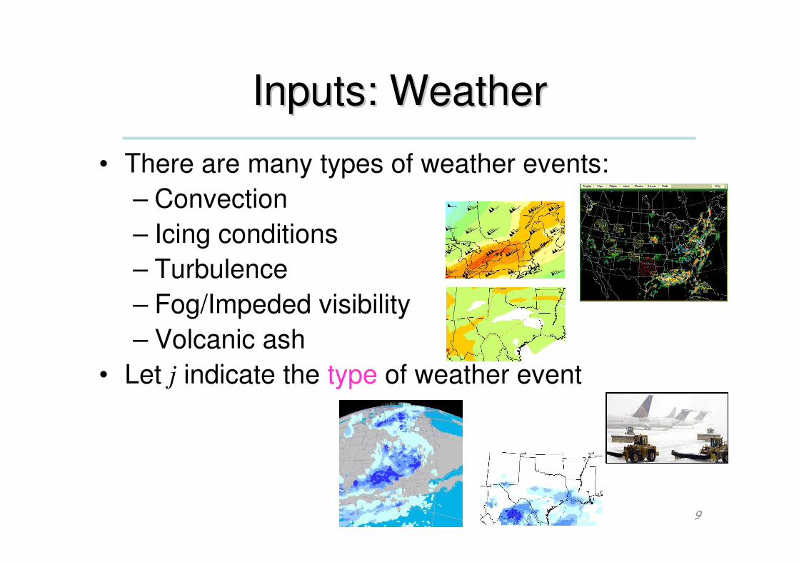
Inputs: WeatherInputs: Weather
• There are many types of weather events:
– Convection
– Icing conditions
– Turbulence
– Fog/Impeded visibility
– Volcanic ash
• Let j indicate the type of weather event
9

Inputs: WeatherInputs: Weather
• Each type j of weather event:
– Wj(x,y,z,t) = intensity at position (x,y,z), time t
– Wj(x,y,z,t) is not known with certainty, but is given by a probabilistic forecast
– Binary impacts: Wj(x,y,z,t) ∈ {0,1}
• Impact region of weather event j for class i aircraft:
– Ii,j(t) = { (x,y,z) : Wj(x,y,z,t) ≥ ξi,j}
• Since impact regions can vary
over time (dynamic weather),
it is best to view impact regions
as portions of space-time.
10
The event either exists or it does not
Convective example

Inputs: WeatherInputs: Weather
• Each type j of weather event may have many forms of
data input that yield the intensity map, Wj(x,y,z,t)
• Example: Icing
11
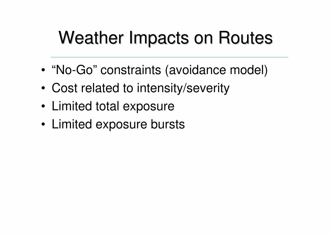
Weather Impacts on RoutesWeather Impacts on Routes
• “No-Go” constraints (avoidance model)
• Cost related to intensity/severity
• Limited total exposure
• Limited exposure bursts

Weather Impacts on Routes: Weather Impacts on Routes: ““NoNo--
GoGo”” ConstraintsConstraints
• Impact regions are “no-go” constraints
– Routes must avoid regions whose intensity
values are above a specified threshold, αi,j .
– Optionally, there is a weather avoidance
threshold, δi,j , specifying a minimum clearance distance a route of equipage class i
should stay from impact regions of weather
type j.
13Hard constraint
δij
Also: Clearance above (in z) echo top

Example: NoExample: No--Go Above a ThresholdGo Above a Threshold
14
a b
intensity
position on route
b
a
threshold
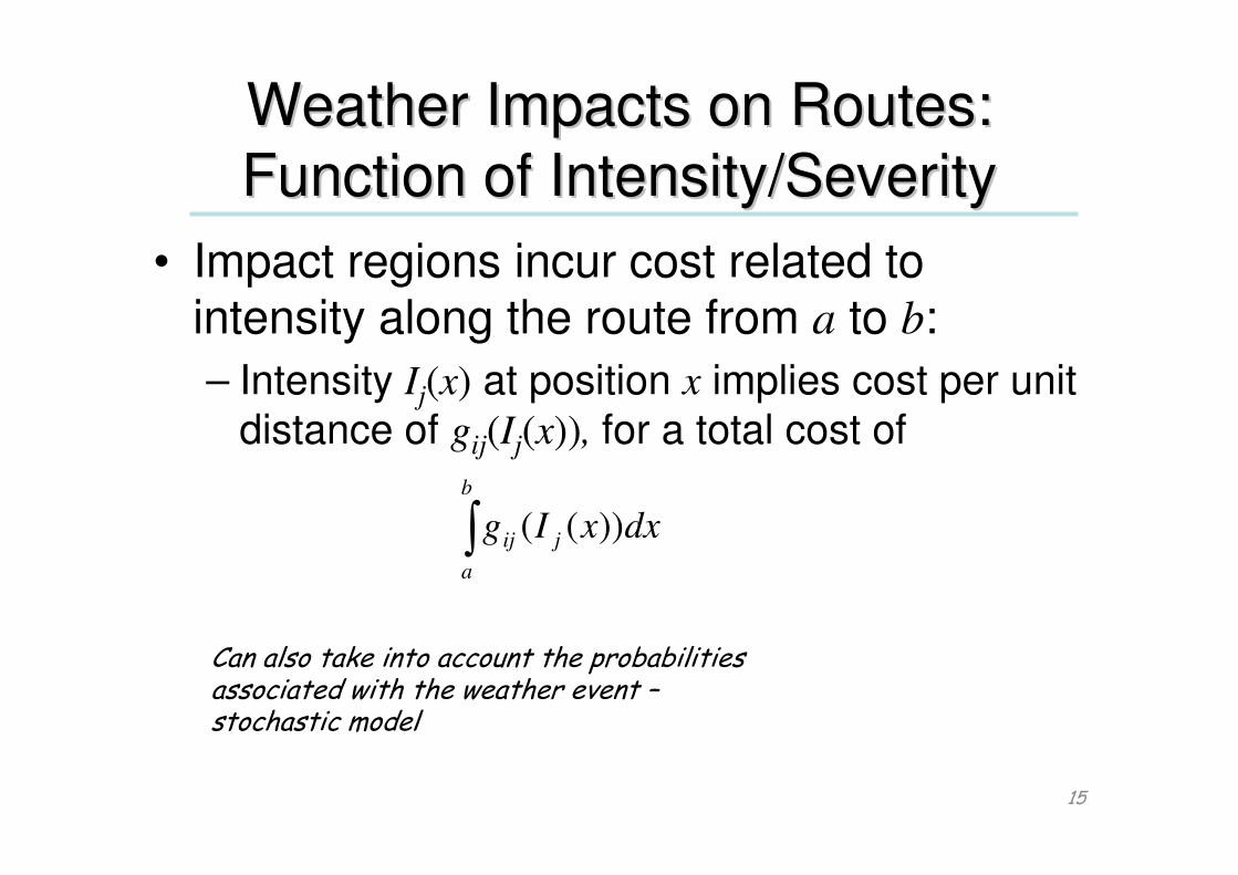
Weather Impacts on Routes: Weather Impacts on Routes:
Function of Intensity/SeverityFunction of Intensity/Severity
• Impact regions incur cost related to intensity along the route from a to b:
– Intensity Ij(x) at position x implies cost per unit
distance of gij(Ij(x)), for a total cost of
15
∫b
a
jij dxxIg ))((
Can also take into account the probabilities associated with the weather event –stochastic model
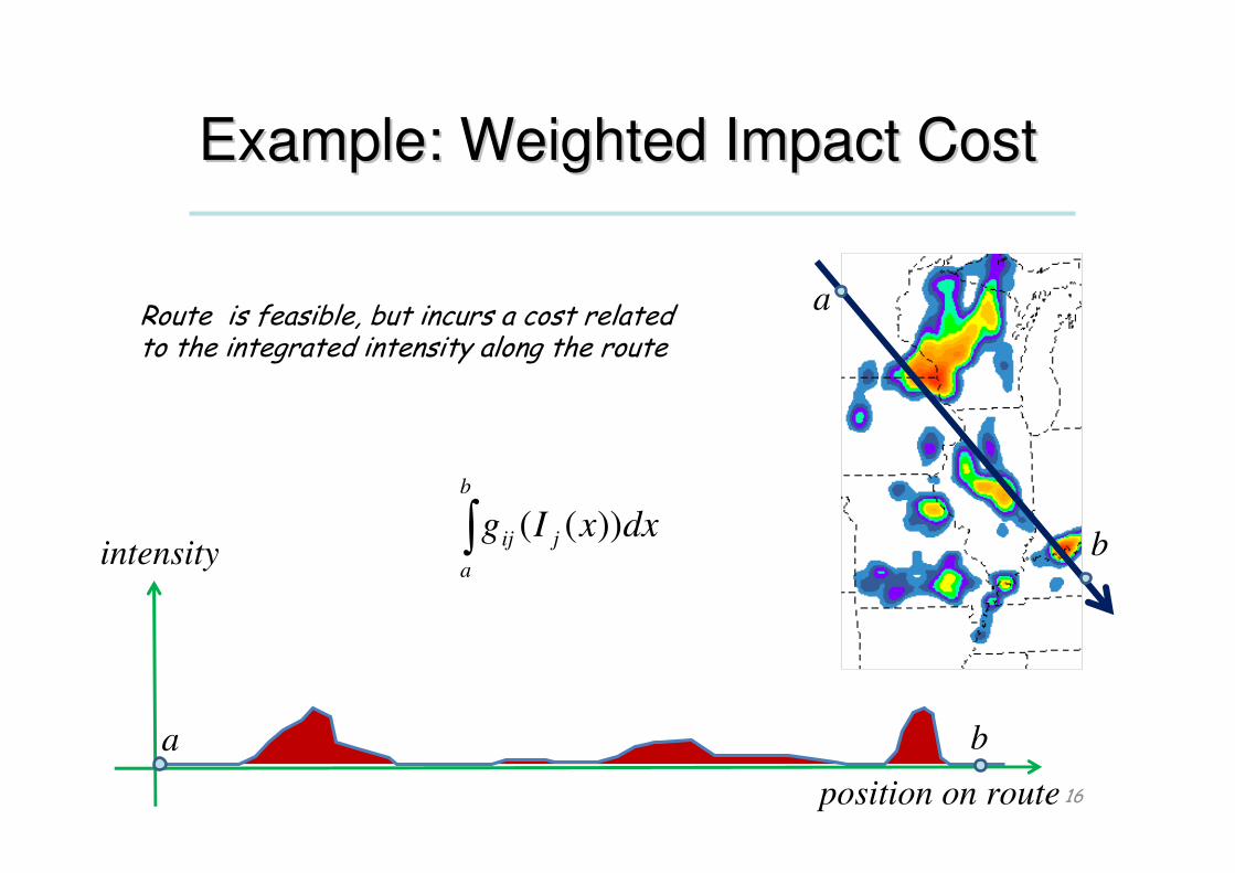
Example: Weighted Impact CostExample: Weighted Impact Cost
16
Route is feasible, but incurs a cost related to the integrated intensity along the route
a b
b
a
intensity
position on route
∫b
a
jij dxxIg ))((
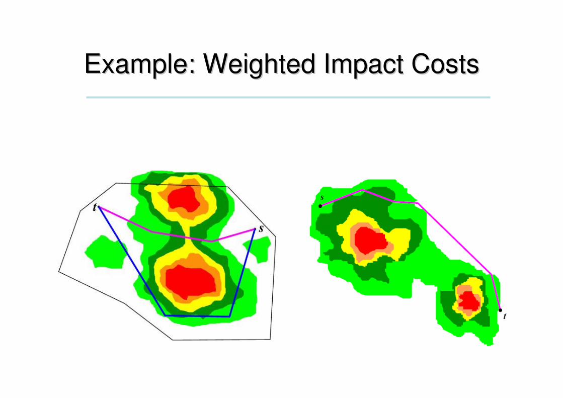
Example: Weighted Impact CostsExample: Weighted Impact Costs
Weather Impacts on Routes: Weather Impacts on Routes:
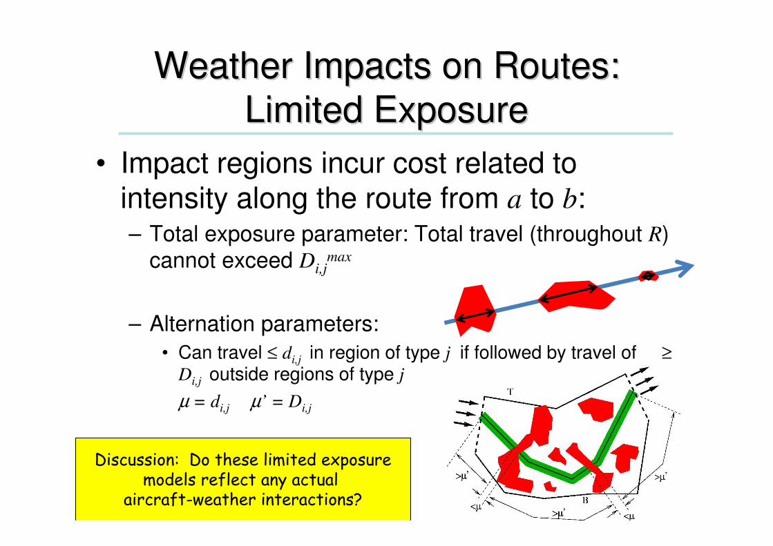
Limited ExposureLimited Exposure
• Impact regions incur cost related to intensity along the route from a to b:– Total exposure parameter: Total travel (throughout R)
cannot exceed Di,jmax
– Alternation parameters:
• Can travel ≤ di,j in region of type j if followed by travel of ≥Di,j outside regions of type j
� µ = di,j µ’ = Di,j
18
Discussion: Do these limited exposuremodels reflect any actual
aircraft-weather interactions?
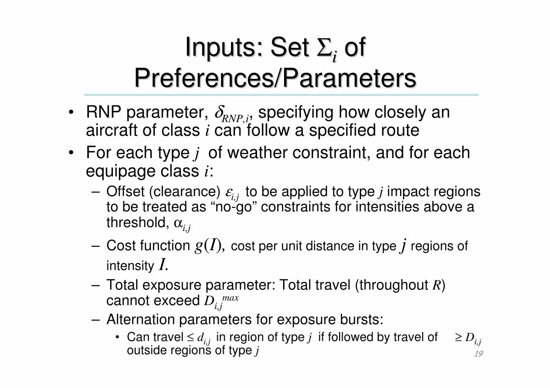
Inputs: Set Inputs: Set ΣΣii of of
Preferences/ParametersPreferences/Parameters• RNP parameter, δRNP,i, specifying how closely an
aircraft of class i can follow a specified route
• For each type j of weather constraint, and for each equipage class i:– Offset (clearance) εi,j to be applied to type j impact regions
to be treated as “no-go” constraints for intensities above a threshold, αi,j
– Cost function g(I), cost per unit distance in type j regions of
intensity I.– Total exposure parameter: Total travel (throughout R)
cannot exceed Di,jmax
– Alternation parameters for exposure bursts:• Can travel ≤ di,j in region of type j if followed by travel of ≥ Di,j
outside regions of type j 19
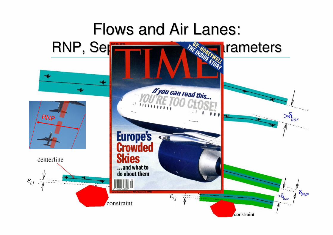
Flows and Air Lanes: Flows and Air Lanes: RNP, Separation, Offset ParametersRNP, Separation, Offset Parameters
εi,j
εi,j
RNPRNP
Model of Hard/Soft ConstraintsModel of Hard/Soft Constraints
• Hard, soft, and everything in between:
– Each class i of aircraft (equipage,
preferences, etc) has an interaction profile
with each type j of weather event
• Weather Impact Interaction Grid
• Multiclass capacity
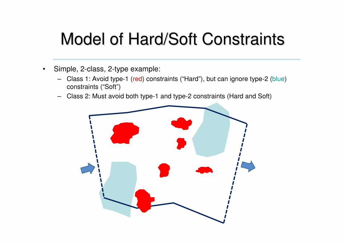
Model of Hard/Soft ConstraintsModel of Hard/Soft Constraints
• Simple, 2-class, 2-type example:
– Class 1: Avoid type-1 (red) constraints (“Hard”), but can ignore type-2 (blue)
constraints (“Soft”)
– Class 2: Must avoid both type-1 and type-2 constraints (Hard and Soft)
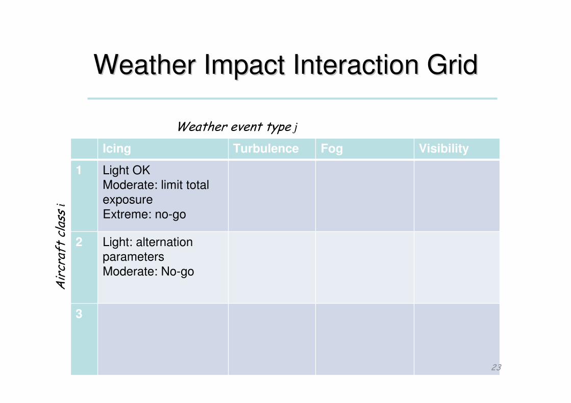
Weather Impact Interaction GridWeather Impact Interaction Grid
Icing Turbulence Fog Visibility
1 Light OK
Moderate: limit total
exposure
Extreme: no-go
2 Light: alternation
parameters
Moderate: No-go
3
23
Weather event type j
Aircraft class
i

Stochastic Model of Weather
• The intensity, Wj(x,y,z,t) , of weather of type j is
not known with certainty, but is given by a
probabilistic forecast
• How to model the random function Wj(x,y,z,t) ?
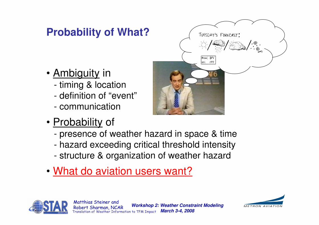
Probability of What?
• Ambiguity in- timing & location
- definition of “event”- communication
• Probability of- presence of weather hazard in space & time
- hazard exceeding critical threshold intensity- structure & organization of weather hazard
• What do aviation users want?
Workshop 2: Weather Constraint Modeling
March 3-4, 2008
Matthias Steiner and Robert Sharman, NCARTranslation of Weather Information to TFM Impact
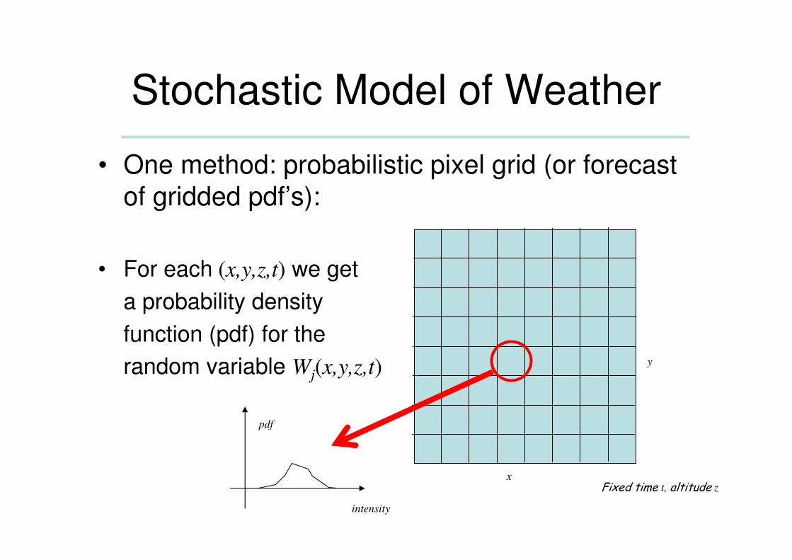
Stochastic Model of Weather
• One method: probabilistic pixel grid (or forecast
of gridded pdf’s):
• For each (x,y,z,t) we get
a probability density
function (pdf) for the
random variable Wj(x,y,z,t)
Fixed time t, altitude z
intensity
x
y

Stochastic Model of Weather
• Another method: Ensemble of forecasts
Forecast: F1
p1
F2
p2
F3
p3
F4
p4Probability:
Discussion: How many? How to assess prior probabilities?

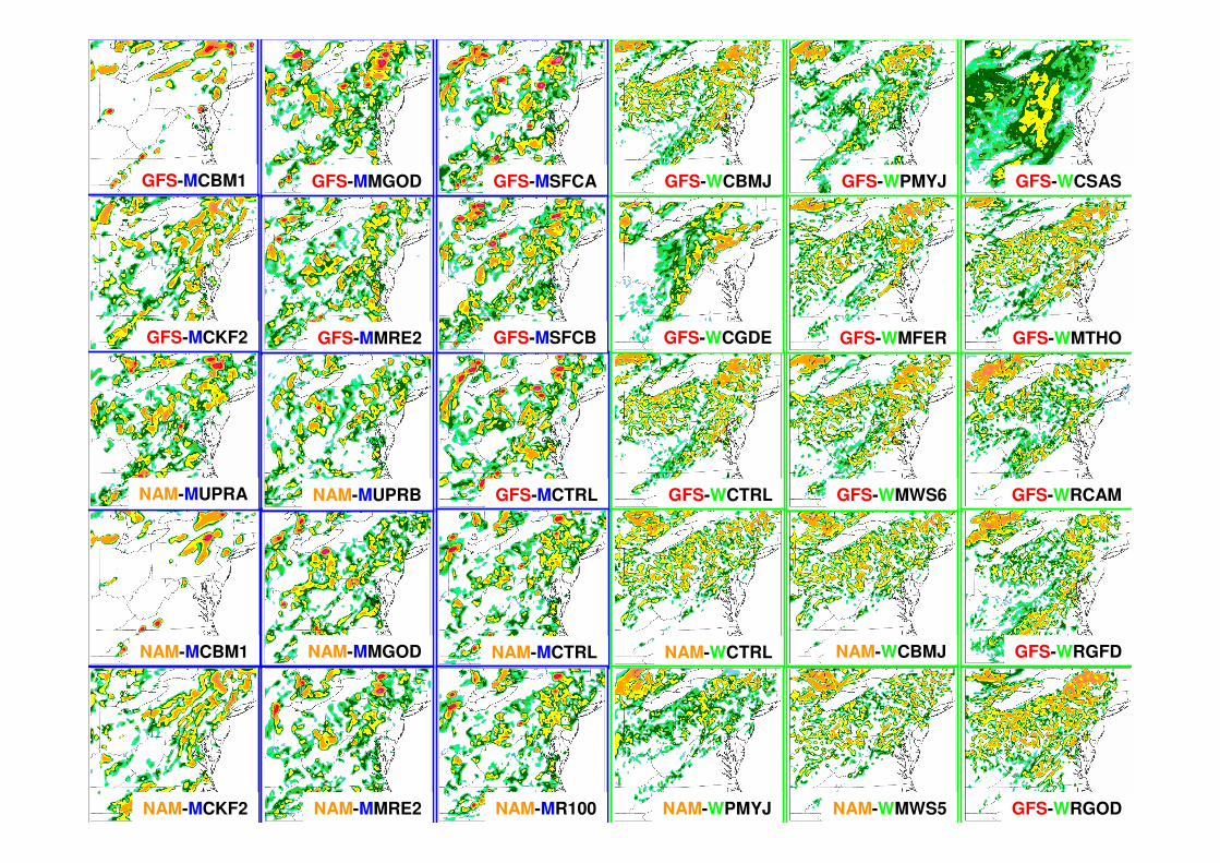
Stochastic Models: Ensembles
Space of all possible forecasts F: probabilities p(F)

Ellrod1
DTF3
FRNTGth
UBF
CLIMO
TEMPG
NCSU1
NCSU2
EDRS10
VWS - NVA - SATRi
GTG20060204 i18 f006
Merging a variety
of turbulence diagnostics
into GTG
provide a measure of“forecast confidence”
6 h forecast valid at 5 Feb 2006 00Z
Flight level: 350
Workshop 2: Weather Constraint Modeling
March 3-4, 2008
Matthias Steiner and Robert Sharman, NCARTranslation of Weather Information to TFM Impact

9 h Ensemble Forecastvalid for
27 June 2007 at 21 UTC
Observation
Ensemble Mean Standard Deviation
1-h Precipitation Accumulation [mm]
Workshop 2: Weather Constraint Modeling
March 3-4, 2008
Matthias Steiner and Robert Sharman, NCARTranslation of Weather Information to TFM Impact
GFS-MCTRL GFS-WCTRL
NAM-MCTRL NAM-WCTRL
GFS-MCBM1
NAM-MCBM1
GFS-WCBMJ
NAM-WCBMJ
GFS-MCKF2
NAM-MCKF2
GFS-WPMYJ
NAM-WPMYJ
GFS-MMGOD
NAM-MMGOD
GFS-MMRE2
NAM-MMRE2
GFS-MSFCA
GFS-MSFCB
NAM-MUPRA
NAM-MR100
NAM-MUPRB
NAM-WMWS5
GFS-WCGDE
GFS-WCSAS
GFS-WMFER GFS-WMTHO
GFS-WMWS6 GFS-WRCAM
GFS-WRGFD
GFS-WRGOD

GFS-MCBM1 GFS-MMGOD GFS-MSFCA GFS-WCBMJ GFS-WPMYJ GFS-WCSAS
GFS-MCKF2 GFS-MMRE2 GFS-MSFCB GFS-WCGDE GFS-WMFER GFS-WMTHO
NAM-MUPRA NAM-MUPRB GFS-MCTRL GFS-WCTRL GFS-WMWS6 GFS-WRCAM
NAM-MCBM1 NAM-MMGOD NAM-MCTRL NAM-WCTRL NAM-WCBMJ GFS-WRGFD
NAM-MCKF2 NAM-MMRE2 NAM-MR100 NAM-WPMYJ NAM-WMWS5 GFS-WRGOD
Turbulence at F
light L
evel 350
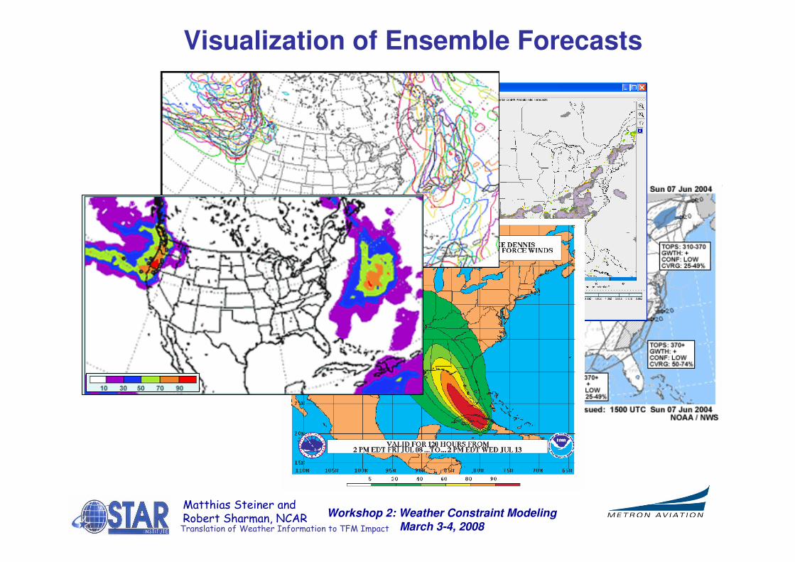
Visualization of Ensemble Forecasts
Workshop 2: Weather Constraint Modeling
March 3-4, 2008
Matthias Steiner and Robert Sharman, NCARTranslation of Weather Information to TFM Impact
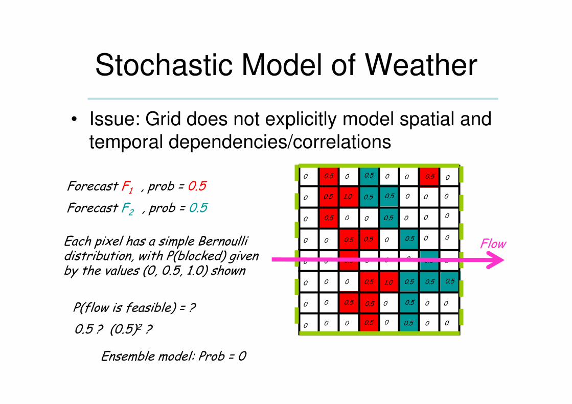
Stochastic Model of Weather
• Issue: Grid does not explicitly model spatial and
temporal dependencies/correlations
Forecast F1 , prob = 0.5
Forecast F2 , prob = 0.5
0.5
0.5
0.5
1.0
0
0
0
0
0
0
0
0
0
0
0
0
0
0
0
0
0
0
0 0 0
0
0
0
00
0
0 0
0
0
000
0
0
0
0
0 0
1.0
0.5
0.5
0.5
0.5
0.5
0.50.5
0.5
0.5
0.5 0.5
0.50.5
0.5
0.5
0.5 0.5
0.5
0.5Each pixel has a simple Bernoulli distribution, with P(blocked) given by the values (0, 0.5, 1.0) shown
P(flow is feasible) = ?
Flow
0.5 ? (0.5)2 ?
Ensemble model: Prob = 0
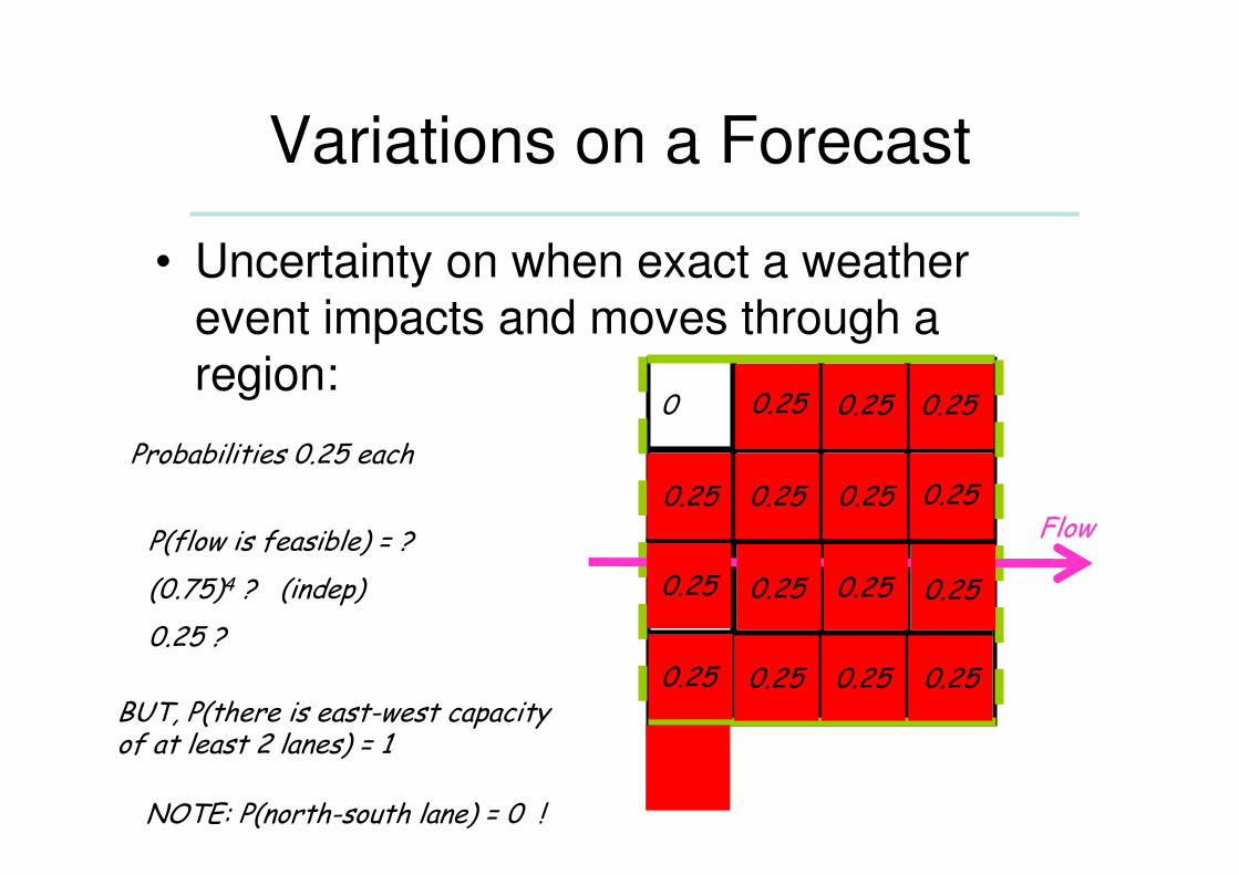
Variations on a Forecast
• Uncertainty on when exact a weather event impacts and moves through a region:
Flow
Probabilities 0.25 each
0.250.25
0.250.250.25
0.250.250.250
0.250.250.250.25
0.250.25
0.25
P(flow is feasible) = ?
(0.75)4 ? (indep)
0.25 ?
BUT, P(there is east-west capacity of at least 2 lanes) = 1
NOTE: P(north-south lane) = 0 !
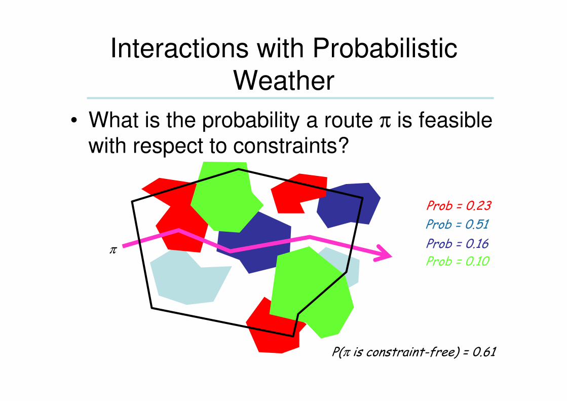
Interactions with Probabilistic
Weather
• What is the probability a route π is feasible with respect to constraints?
Prob = 0.23
Prob = 0.51
Prob = 0.16π
P(π is constraint-free) = 0.61
Prob = 0.10

Variations on Forecast
Seed location:
∆T = 0, p=0.5
∆T = 1, p=0.2
∆T = 2, p=0.15
∆T = 3, p=0.15
p(∆T)
∆T

Capacity Estimation: Probabilistic
Weather
• For capacity estimation, exact shape of weather impact region is not as significant as its “porosity”
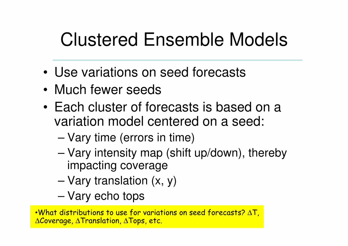
Clustered Ensemble Models
• Use variations on seed forecasts
• Much fewer seeds
• Each cluster of forecasts is based on a variation model centered on a seed:– Vary time (errors in time)
– Vary intensity map (shift up/down), thereby impacting coverage
– Vary translation (x, y)
– Vary echo tops
•What distributions to use for variations on seed forecasts? ∆T, ∆Coverage, ∆Translation, ∆Tops, etc.


