26
Baseline New-Keynesian Model Optimal Monetary Policy (Short version)
Baseline New-Keynesian ModelOptimal Monetary Policy
(Short version)
Motivation
Generally accepted principle: policymakers should act in an optimal manner, i.e. maximize welfare for representative household
DSGE models enable one to
• compare different policy rules
• compute optimal policies (given a pre-defined objective)
• quantify welfare gain/loss of different policies and instruments
Canonical New-Keynesian Model
Two sources of distortions/inefficiencies
• Market power due to monopolistically competitive firms
• Relative price distortions resulting from staggered price setting
Inefficiencies are analytically tractable and quantifiable
Optimal allocation is equal to undistorted flex-price allocation
Definitions
Efficient output : Level of output that would prevail under perfect competition
Natural output : Level of output that would prevail under imperfect competition, but flexible prices and wages
yet
ynt
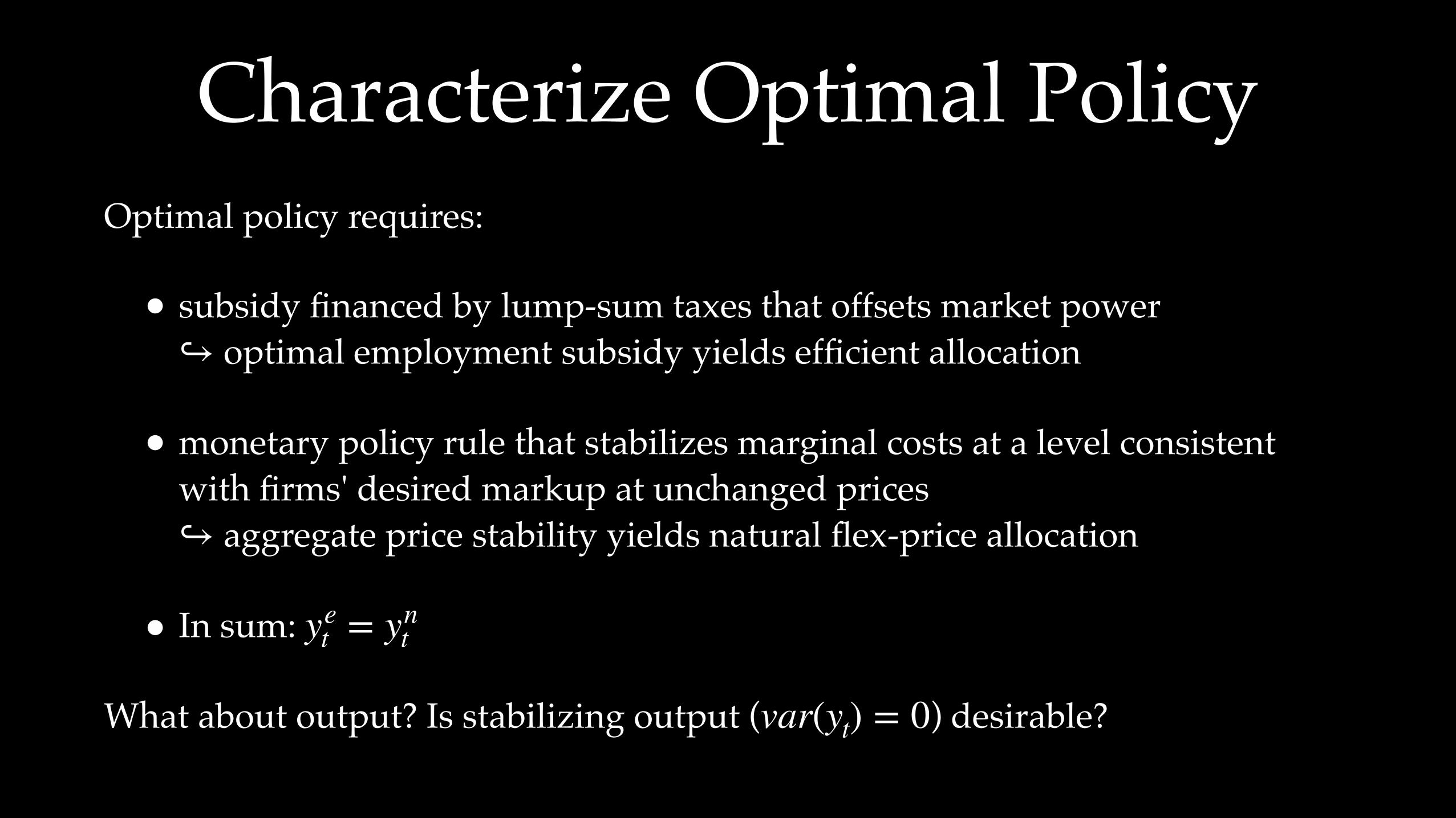
Characterize Optimal PolicyOptimal policy requires:
• subsidy financed by lump-sum taxes that offsets market power optimal employment subsidy yields efficient allocation
• monetary policy rule that stabilizes marginal costs at a level consistent with firms' desired markup at unchanged prices
aggregate price stability yields natural flex-price allocation
• In sum:
What about output? Is stabilizing output ( ) desirable?
↪
↪
yet = yn
t
var(yt) = 0
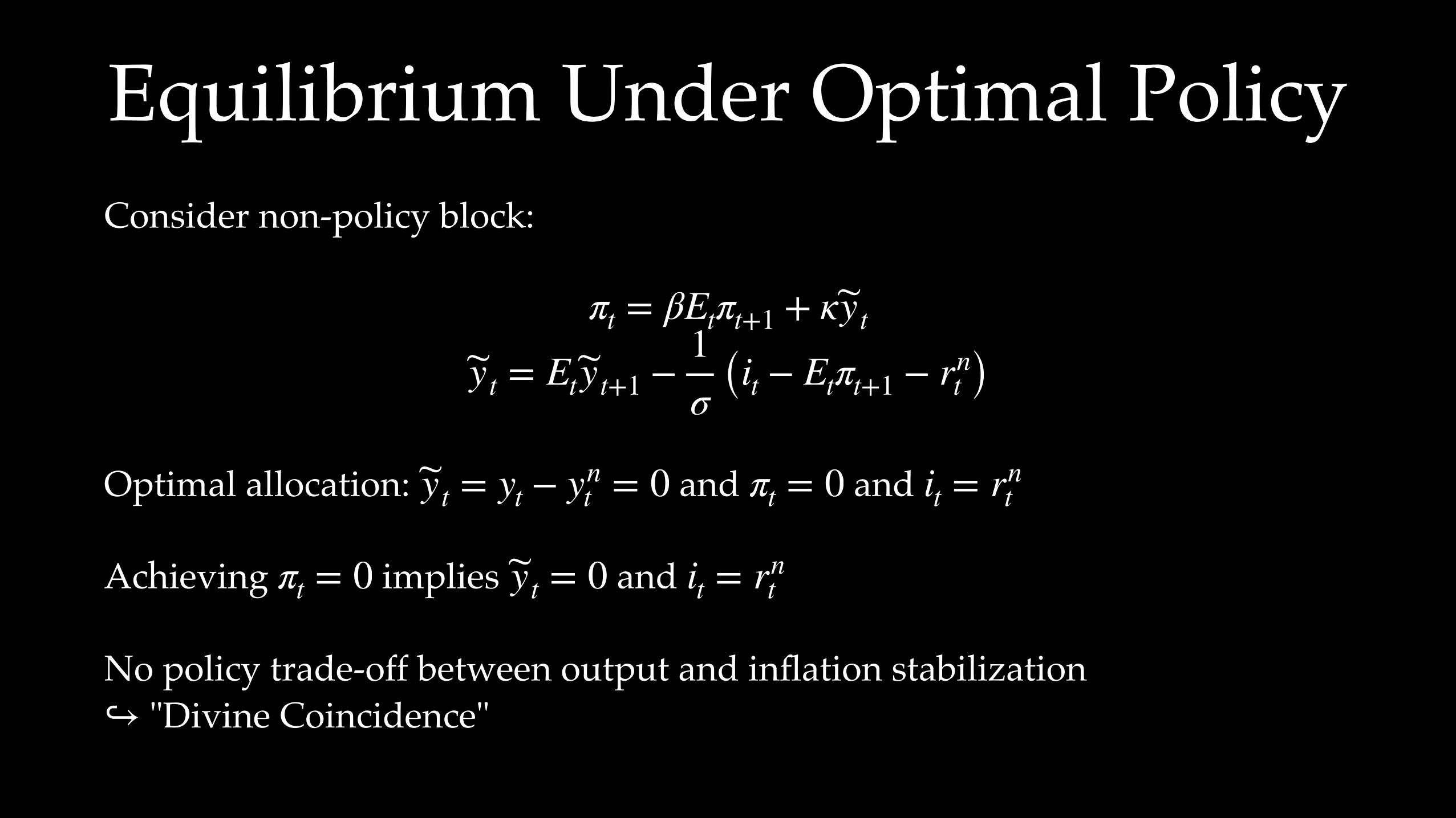
Equilibrium Under Optimal PolicyConsider non-policy block:
Optimal allocation: and and
Achieving implies and
No policy trade-off between output and inflation stabilization "Divine Coincidence"
πt = βEtπt+1 + κyt
yt = Etyt+1 −1σ (it − Etπt+1 − rn
t )
yt = yt − ynt = 0 πt = 0 it = rn
t
πt = 0 yt = 0 it = rnt
↪
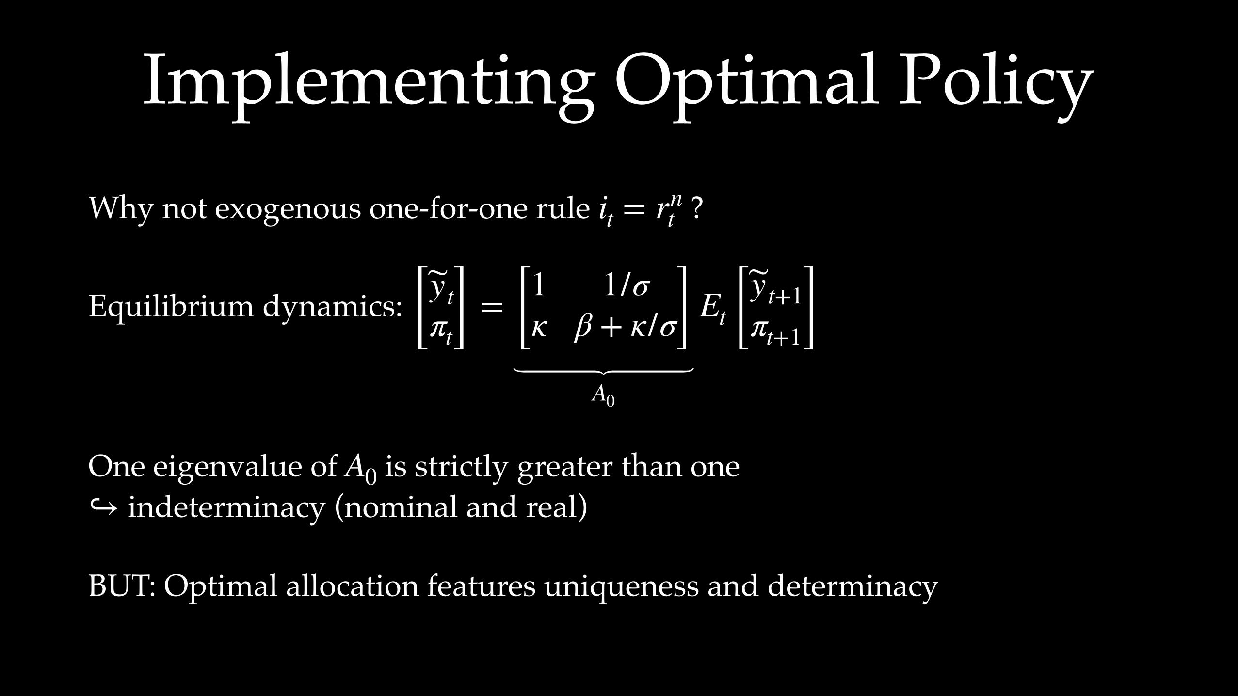
Implementing Optimal PolicyWhy not exogenous one-for-one rule ?
Equilibrium dynamics:
One eigenvalue of is strictly greater than one indeterminacy (nominal and real)
BUT: Optimal allocation features uniqueness and determinacy
it = rnt
[ytπt] = [1 1/σ
κ β + κ/σ]A0
Et [yt+1πt+1]
A0↪
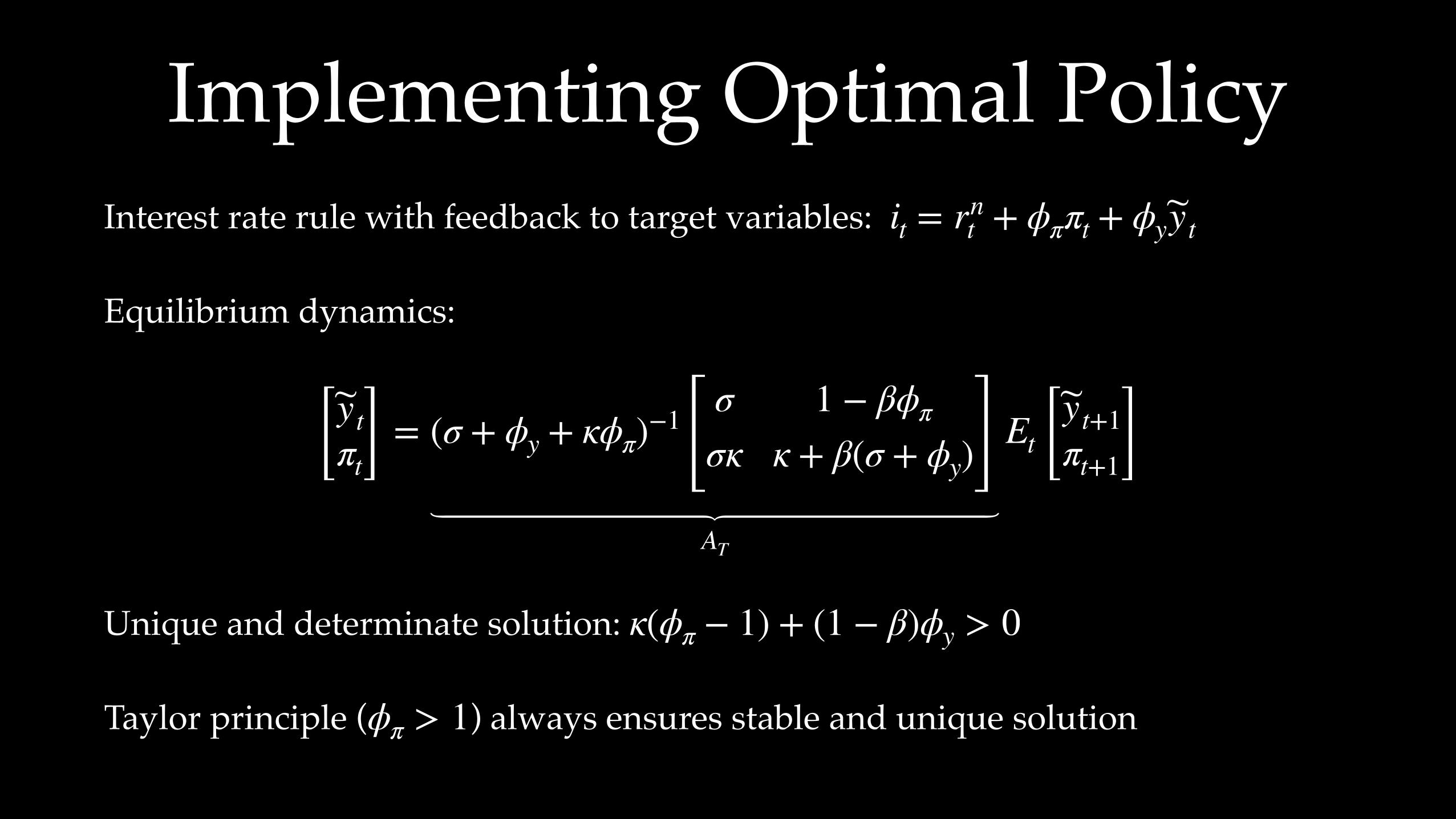
Implementing Optimal PolicyInterest rate rule with feedback to target variables:
Equilibrium dynamics:
Unique and determinate solution:
Taylor principle ( ) always ensures stable and unique solution
it = rnt + ϕππt + ϕyyt
[ytπt] = (σ + ϕy + κϕπ)−1[
σ 1 − βϕπ
σκ κ + β(σ + ϕy)]AT
Et [yt+1πt+1]
κ(ϕπ − 1) + (1 − β)ϕy > 0
ϕπ > 1
Policy Trade-OffsIn reality policy makers face trade-offs (at least in the short-run) due to several sources of uncertainty and frictions
Usually central bankers commit to medium-term inflation target, but also want to avoid excessive instability of output and employment
But: do they commit to their plans?
• Commitment: make state-contingent policy plan, bound by past promises
• Discretion: make decision each period, don't feel bound by past promises
Farewell Divine Coincidence
Definitions:
• Efficient output : Level of output that would prevail under perfect competition
• Natural output : Level of output that would prevail under imperfect competition, but flexible prices and wages
Nominal rigidities AND real frictions break divine coincidence as flex-price allocation is inefficient and not optimal to target
yet
ynt
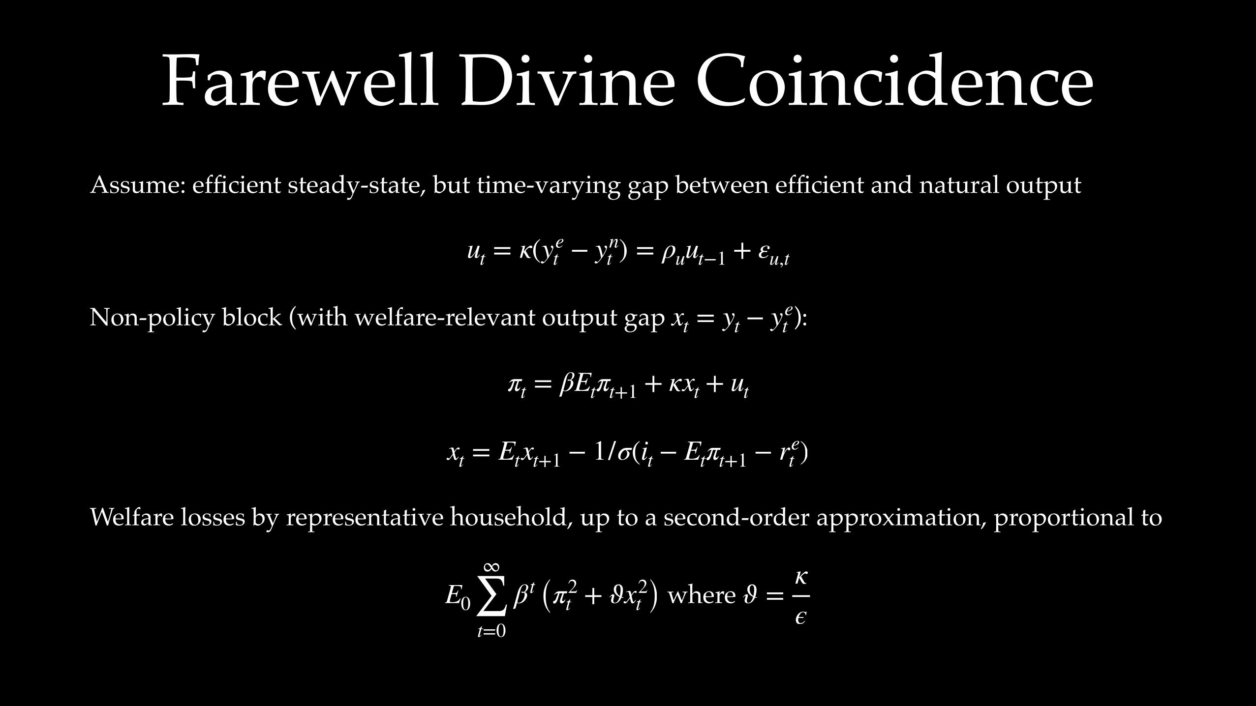
Farewell Divine CoincidenceAssume: efficient steady-state, but time-varying gap between efficient and natural output
Non-policy block (with welfare-relevant output gap ):
Welfare losses by representative household, up to a second-order approximation, proportional to
where
ut = κ(yet − yn
t ) = ρuut−1 + εu,t
xt = yt − yet
πt = βEtπt+1 + κxt + ut
xt = Etxt+1 − 1/σ(it − Etπt+1 − ret )
E0
∞
∑t=0
βt (π2t + ϑx2
t ) ϑ =κϵ
Ramsey ProblemSocial planner maximizes objective function or minimizes loss function by choosing specific policy instrument and taking into account the equilibrium conditions of the economy
FOC of social planner's problem and equilibrium conditions form a system of equations with
• endogenous variables
• policy instrument(s)
• Lagrangian multipliers of the social planner's problem
• initial conditions
Linearized system then enables one to compute e.g. impulse responses to a given shock
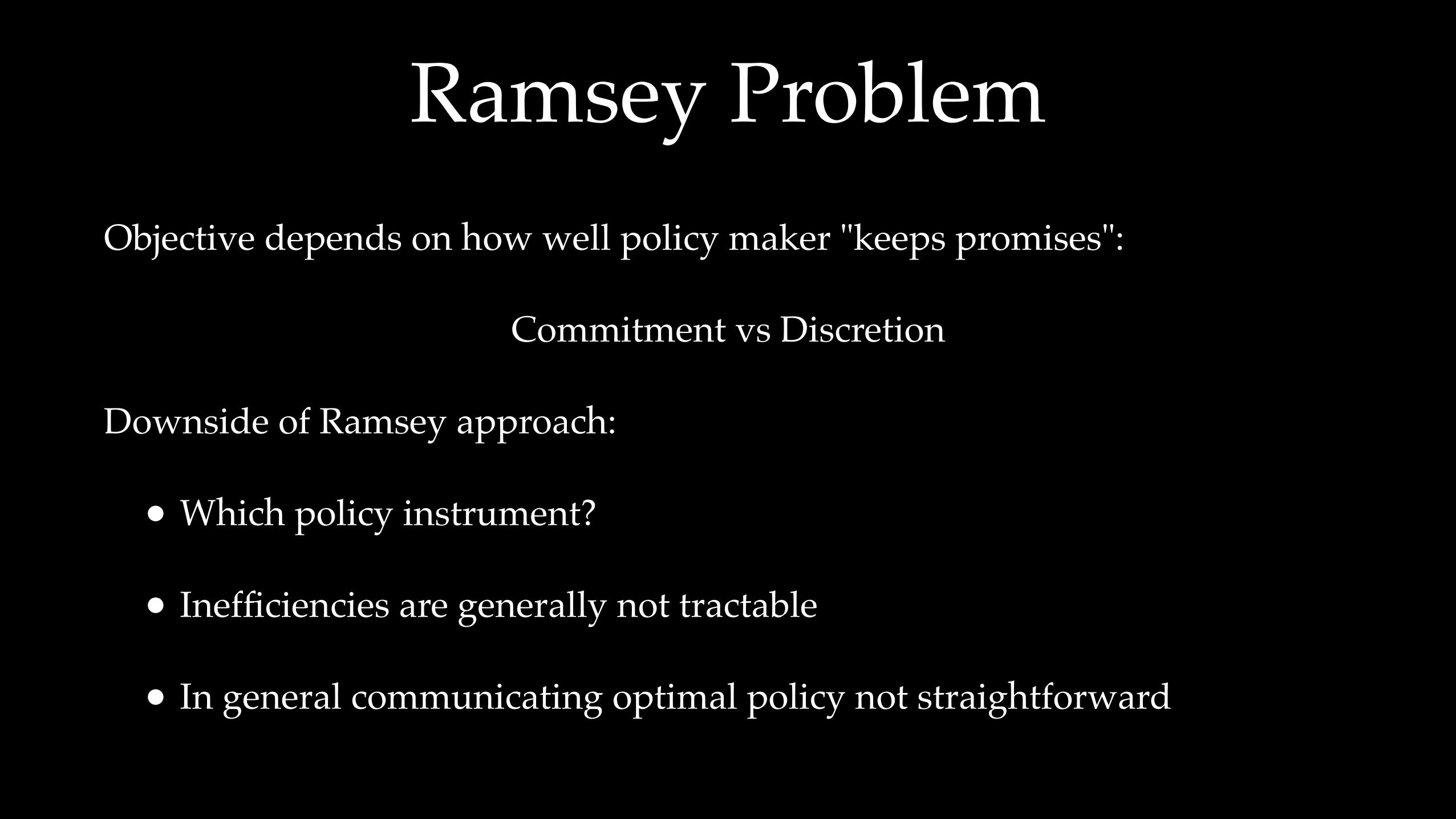
Ramsey ProblemObjective depends on how well policy maker "keeps promises":
Commitment vs Discretion
Downside of Ramsey approach:
• Which policy instrument?
• Inefficiencies are generally not tractable
• In general communicating optimal policy not straightforward
Ramsey Problem
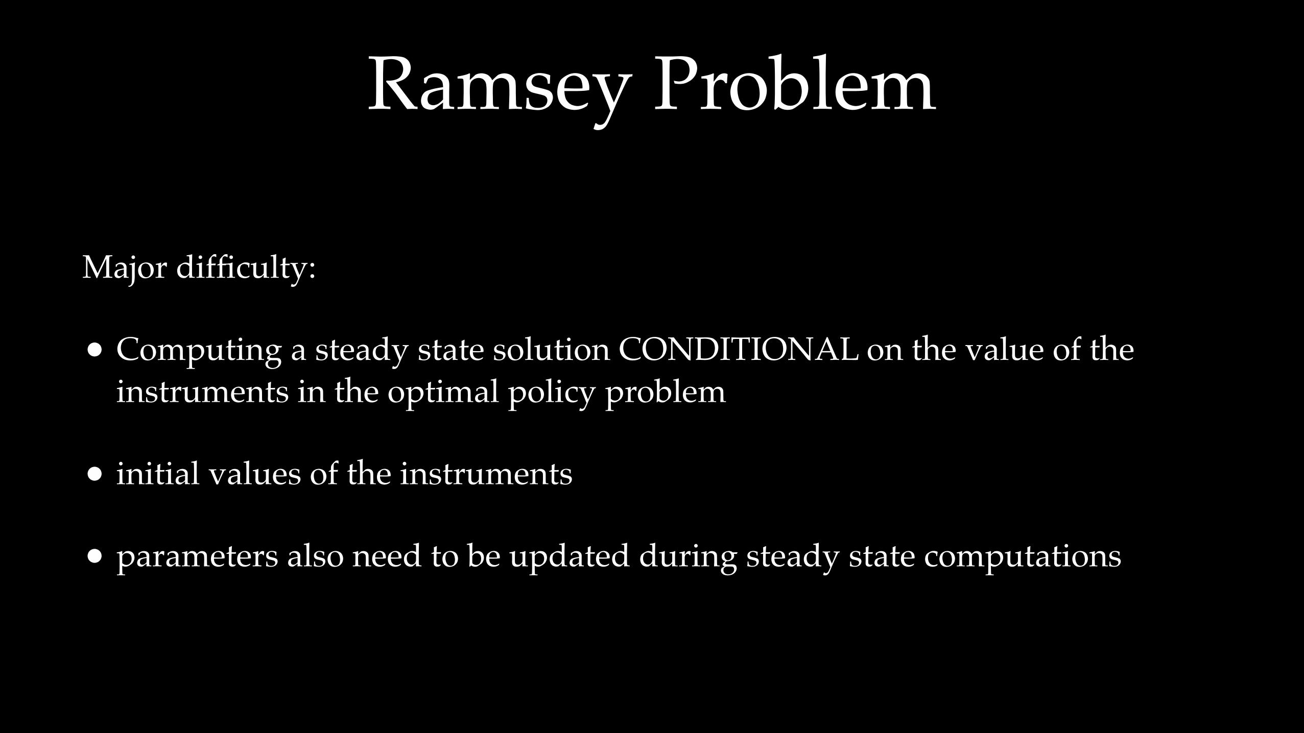
Major difficulty:
• Computing a steady state solution CONDITIONAL on the value of the instruments in the optimal policy problem
• initial values of the instruments
• parameters also need to be updated during steady state computations
Optimal Policy Under Commitment
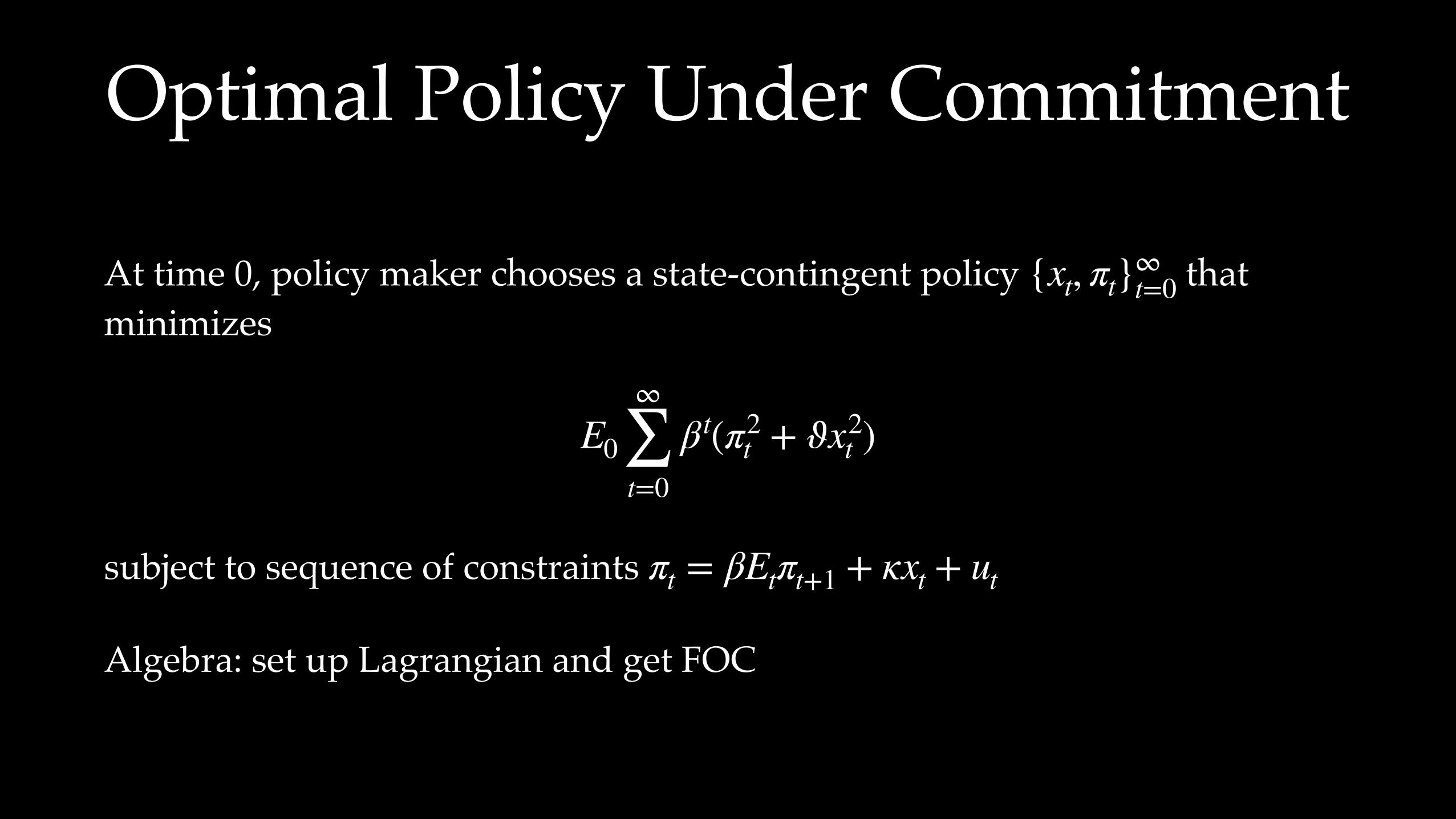
At time 0, policy maker chooses a state-contingent policy that minimizes
subject to sequence of constraints
Algebra: set up Lagrangian and get FOC
{xt, πt}∞t=0
E0
∞
∑t=0
βt(π2t + ϑx2
t )
πt = βEtπt+1 + κxt + ut
Optimal Policy Under Commitment Dynare Commands
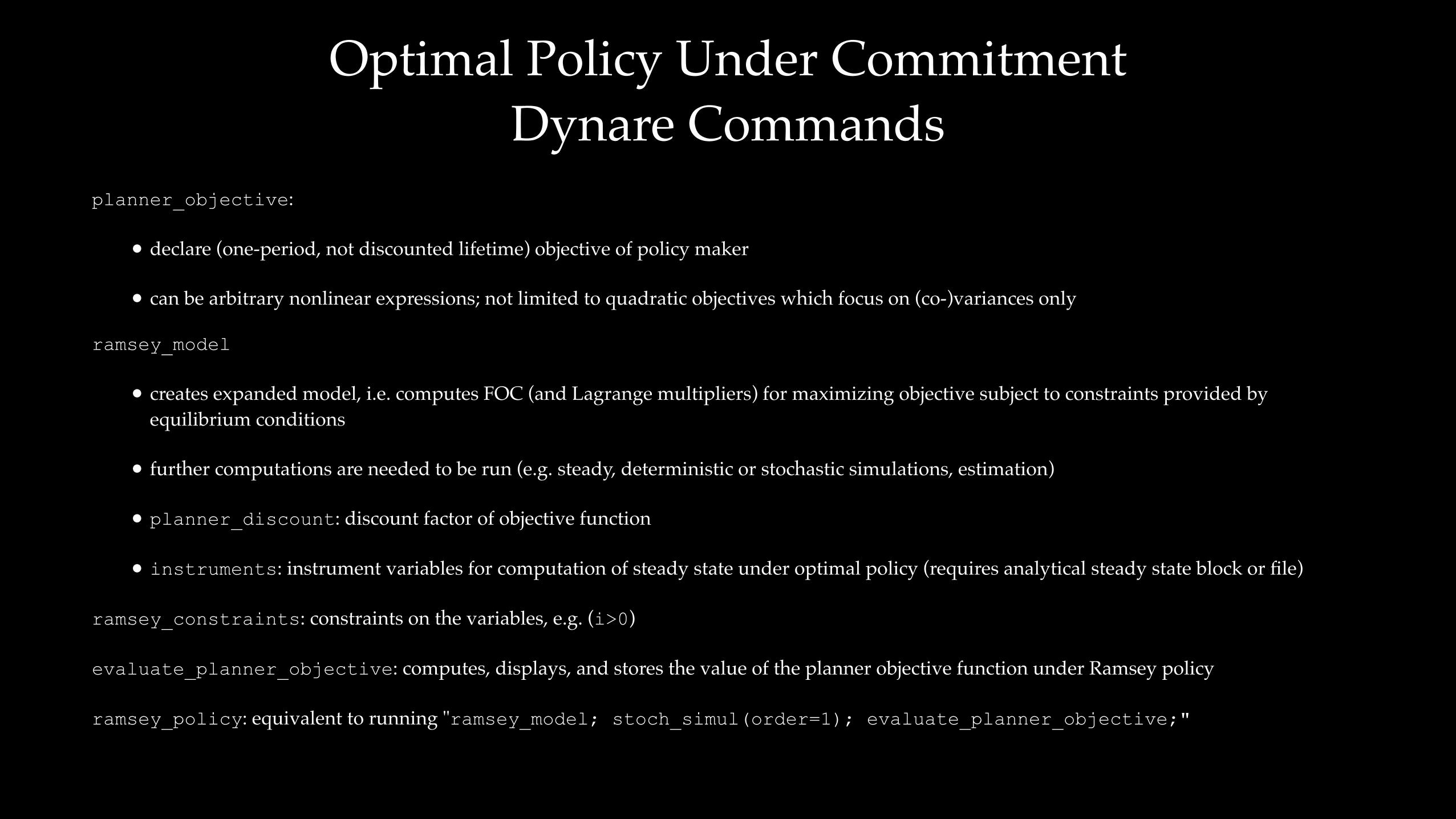
planner_objective:
• declare (one-period, not discounted lifetime) objective of policy maker
• can be arbitrary nonlinear expressions; not limited to quadratic objectives which focus on (co-)variances only
ramsey_model
• creates expanded model, i.e. computes FOC (and Lagrange multipliers) for maximizing objective subject to constraints provided by equilibrium conditions
• further computations are needed to be run (e.g. steady, deterministic or stochastic simulations, estimation)
• planner_discount: discount factor of objective function
• instruments: instrument variables for computation of steady state under optimal policy (requires analytical steady state block or file)
ramsey_constraints: constraints on the variables, e.g. (i>0)
evaluate_planner_objective: computes, displays, and stores the value of the planner objective function under Ramsey policy
ramsey_policy: equivalent to running "ramsey_model; stoch_simul(order=1); evaluate_planner_objective;"
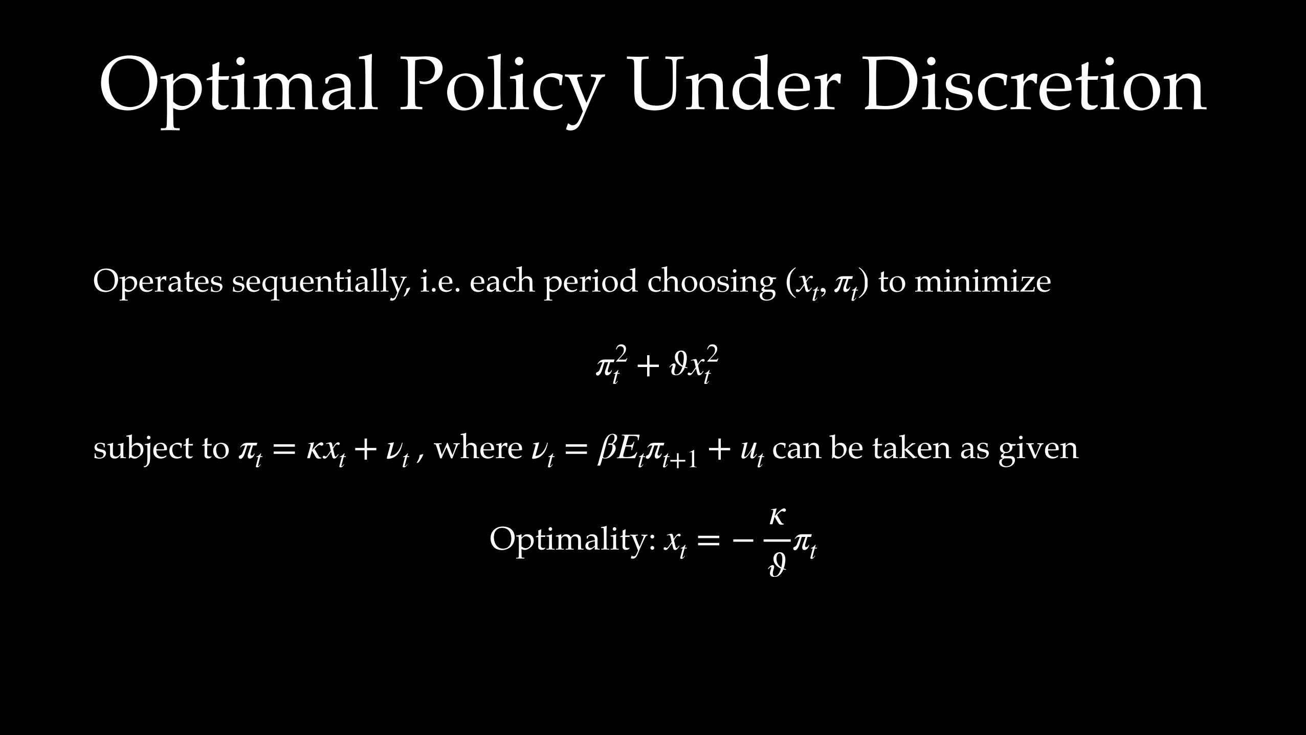
Optimal Policy Under Discretion
Operates sequentially, i.e. each period choosing to minimize
subject to , where can be taken as given
Optimality:
(xt, πt)
π2t + ϑx2
t
πt = κxt + νt νt = βEtπt+1 + ut
xt = −κϑ
πt
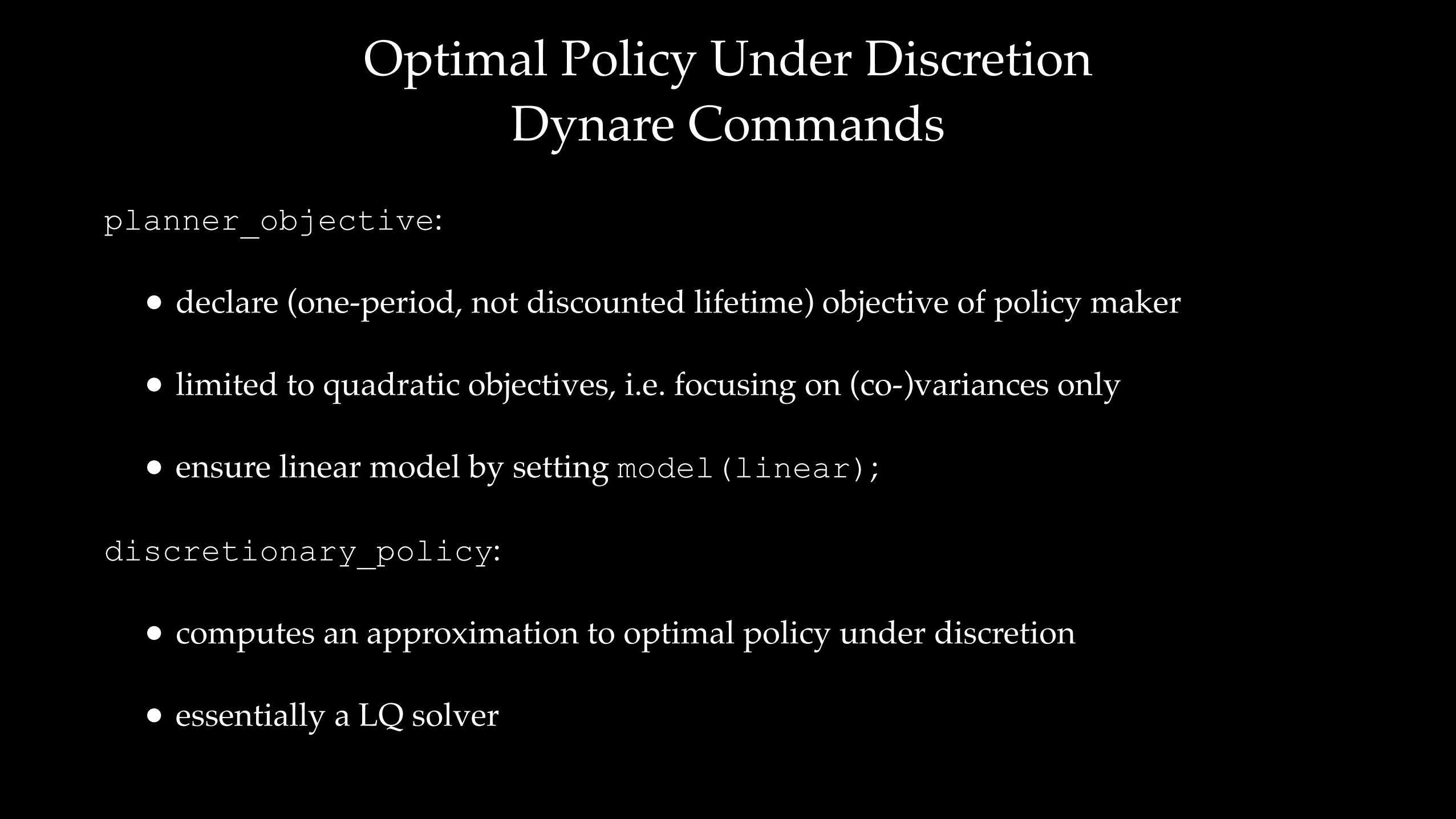
Optimal Policy Under Discretion Dynare Commands
planner_objective:
• declare (one-period, not discounted lifetime) objective of policy maker
• limited to quadratic objectives, i.e. focusing on (co-)variances only
• ensure linear model by setting model(linear);
discretionary_policy:
• computes an approximation to optimal policy under discretion
• essentially a LQ solver
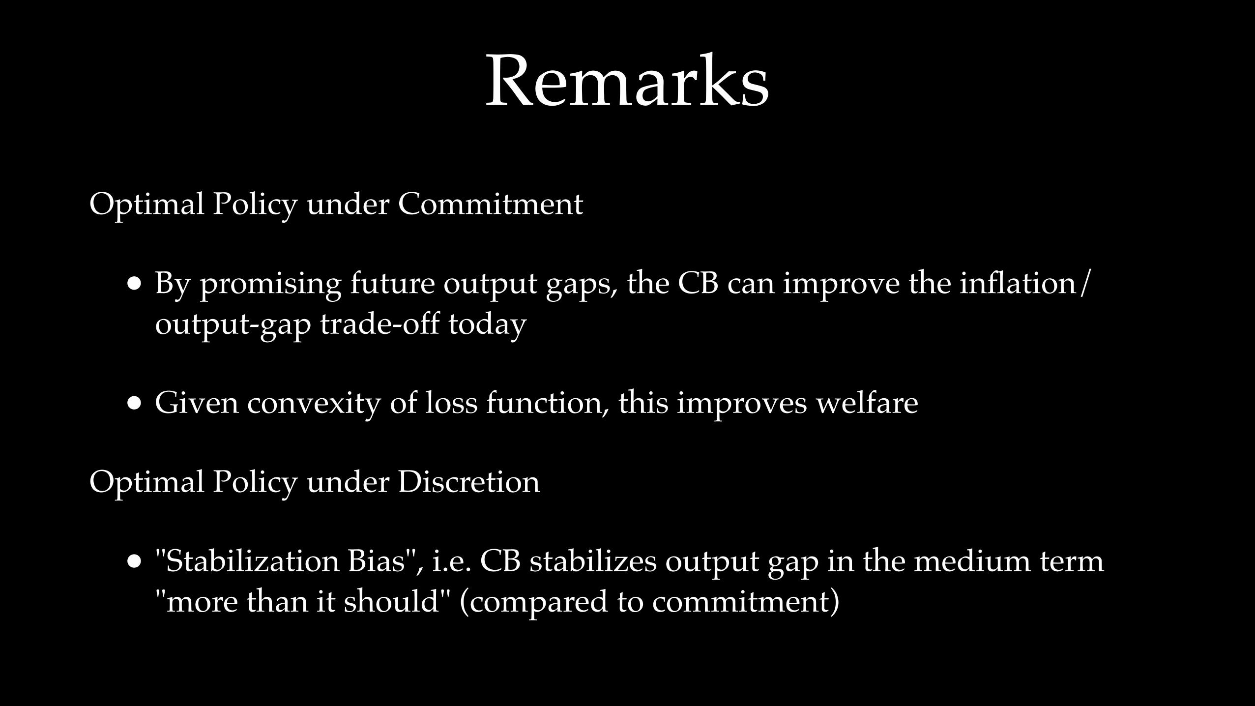
RemarksOptimal Policy under Commitment
• By promising future output gaps, the CB can improve the inflation/output-gap trade-off today
• Given convexity of loss function, this improves welfare
Optimal Policy under Discretion
• "Stabilization Bias", i.e. CB stabilizes output gap in the medium term "more than it should" (compared to commitment)
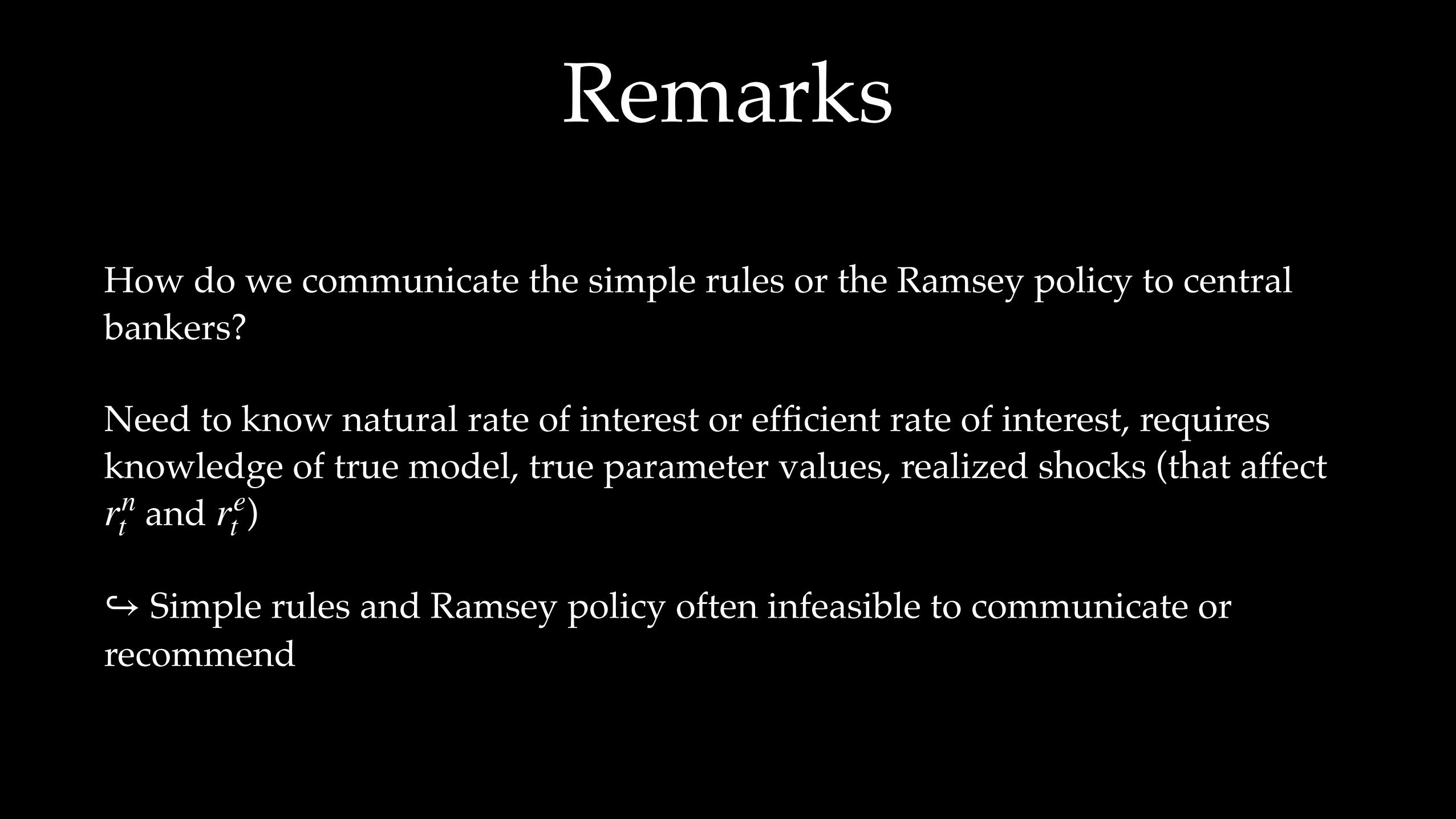
Remarks
How do we communicate the simple rules or the Ramsey policy to central bankers?
Need to know natural rate of interest or efficient rate of interest, requires knowledge of true model, true parameter values, realized shocks (that affect
and )
Simple rules and Ramsey policy often infeasible to communicate or recommend
rnt re
t
↪
Simple Implementable Rules
Alternative: simple implementable rules
• Policy instrument depends on observable variables only
• Do not require knowledge of true parameter values
• Need to come up with an evaluation criteria
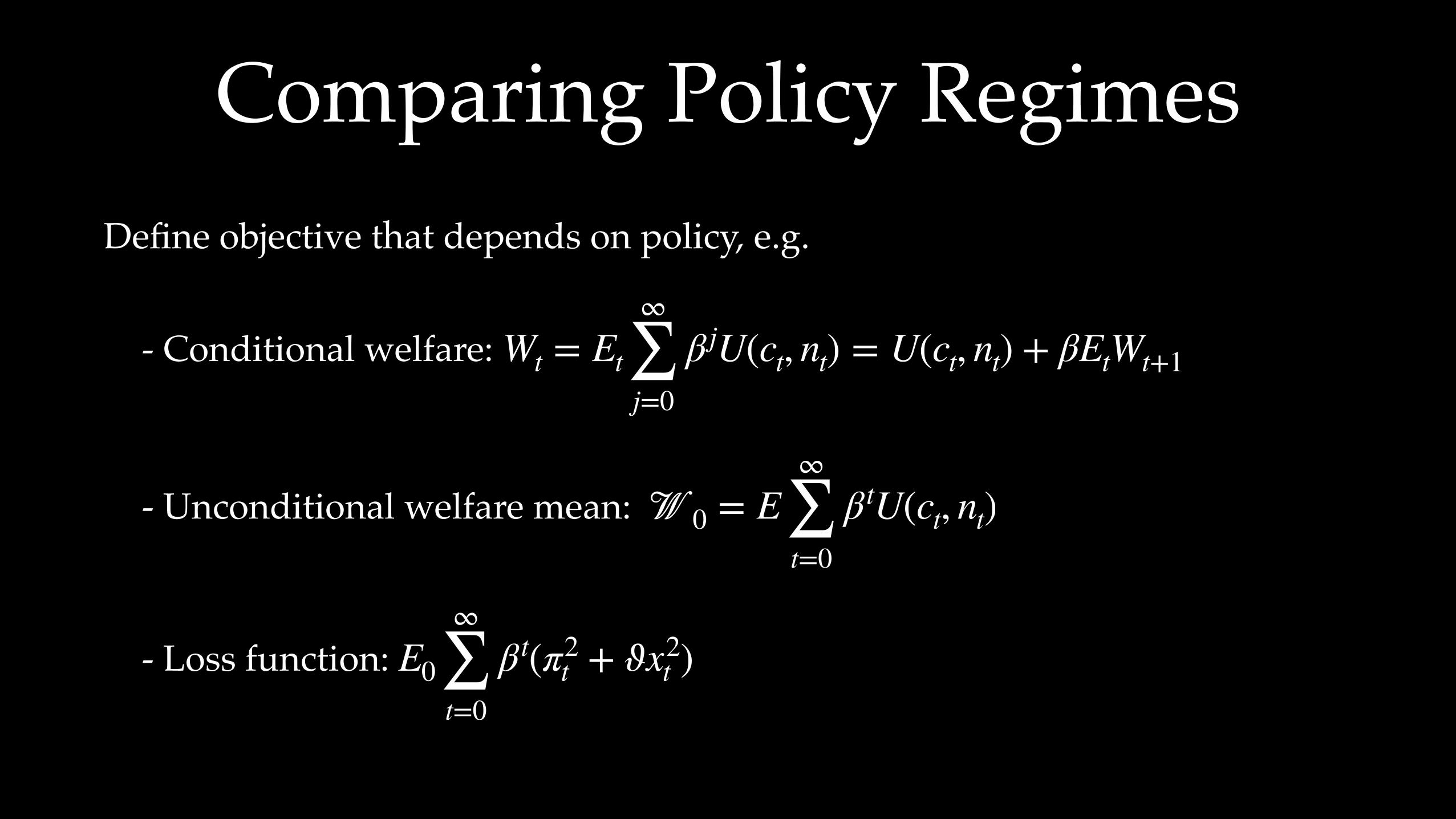
Comparing Policy RegimesDefine objective that depends on policy, e.g.
- Conditional welfare:
- Unconditional welfare mean:
- Loss function:
Wt = Et
∞
∑j=0
β jU(ct, nt) = U(ct, nt) + βEtWt+1
𝒲0 = E∞
∑t=0
βtU(ct, nt)
E0
∞
∑t=0
βt(π2t + ϑx2
t )
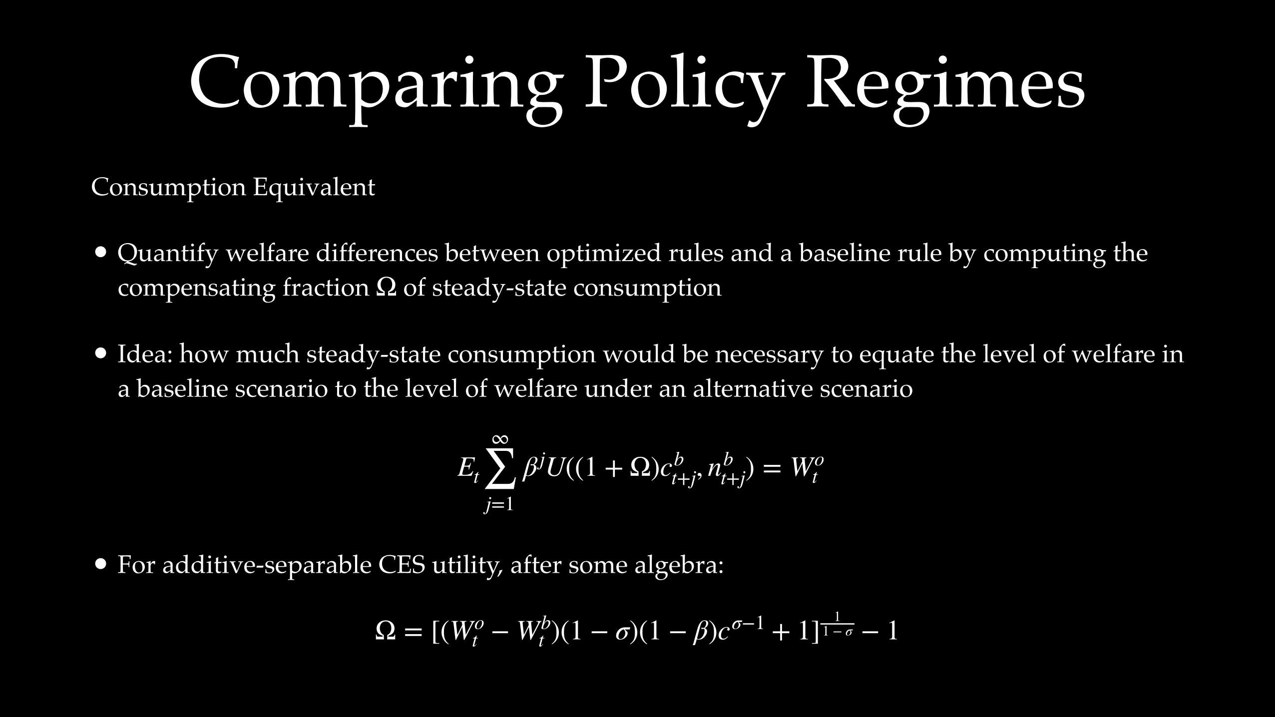
Comparing Policy RegimesConsumption Equivalent
• Quantify welfare differences between optimized rules and a baseline rule by computing the compensating fraction of steady-state consumption
• Idea: how much steady-state consumption would be necessary to equate the level of welfare in a baseline scenario to the level of welfare under an alternative scenario
• For additive-separable CES utility, after some algebra:
Ω
Et
∞
∑j=1
β jU((1 + Ω)cbt+j, nb
t+j) = Wot
Ω = [(Wot − Wb
t )(1 − σ)(1 − β)cσ−1 + 1] 11 − σ − 1
Comparing Policy Regimes
How to compare different policy regimes
• start at same initial condition (e.g. steady-state)
• approximate model to at least 2nd order
• define grid for parameters (e.g. parameters of policy rule)
• search parameters by optimizing objective
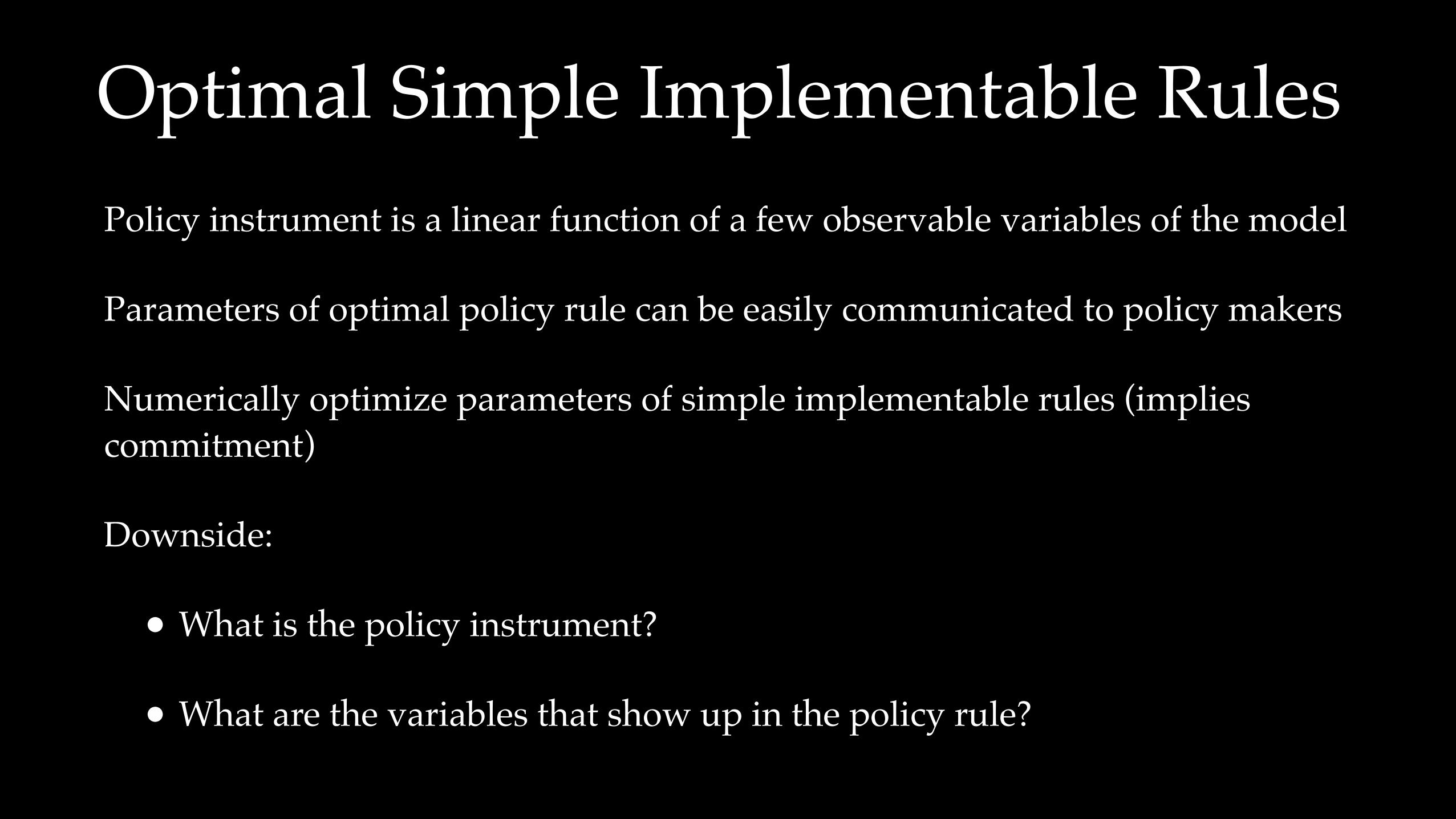
Optimal Simple Implementable RulesPolicy instrument is a linear function of a few observable variables of the model
Parameters of optimal policy rule can be easily communicated to policy makers
Numerically optimize parameters of simple implementable rules (implies commitment)
Downside:
• What is the policy instrument?
• What are the variables that show up in the policy rule?
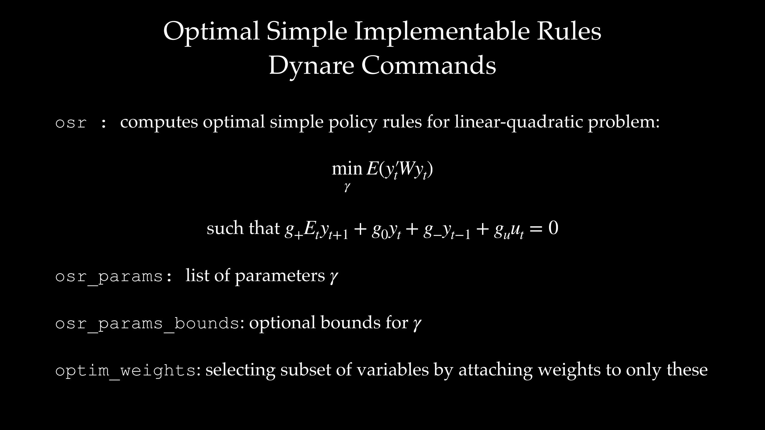
Optimal Simple Implementable Rules Dynare Commands
osr : computes optimal simple policy rules for linear-quadratic problem:
such that
osr_params: list of parameters
osr_params_bounds: optional bounds for
optim_weights: selecting subset of variables by attaching weights to only these
minγ
E(y′ tWyt)
g+Etyt+1 + g0yt + g−yt−1 + guut = 0
γ
γ


![New Keynesian Model[1]](https://static.documents.pub/doc/80x56/577cd6701a28ab9e789c6177/new-keynesian-model1.jpg)


