(1.8)(1.8)

(1.6)(1.6)

(1.4)(1.4)

(1.2)(1.2)

(1.5)(1.5)

(1.7)(1.7)

(1.1)(1.1)

(1.3)(1.3)

Basic arithmetic

Arithmetic expressions can be typed into Maple using the regular operators:

7

5

2 1

(type "3 * 7")

1 33

(type "12 / 9")

386

(type "2 ^ 7")

Maple does know about the usual precedence of operations

1 7

We can use parentheses to alter this

2 7

Arithmetic expressions may contain variables, they remain unevaluated

(1.14)(1.14)

(1.11)(1.11)

(1.16)(1.16)

(1.15)(1.15)

(1.10)(1.10)

(1.13)(1.13)

(1.12)(1.12)

(1.9)(1.9)

(in the document version of Maple we have a choice of typing "5 y" or "5 * y" - Maple accepts both. The command line version only accepts "5 * y". Be careful with the product of variables, however, since (ie, "x [Space] y") and (ie "xy" with no space in between) refer to different things!)

0

Notice that Maple usually does not simplify the terms we enter

(we will see later how we can bring Maple to expand terms like the above).

Maple knows many mathematical functions and constants

0

(Maple automatically simplifies "sin(0)" because the result is a simple number. On the other hand, there is no nicer representation for "cos(1)" than "cos(1)", and so Maple does not simplify it by default.)

(for the symbol type "pi [Esc]" an select the corresponding entry from the menu).

120

e2

(we can also insert the exponential e with "e [Esc]").

(2.5)(2.5)

(2.1)(2.1)

(2.6)(2.6)

(2.4)(2.4)

(1.17)(1.17)

(2.2)(2.2)

(2.3)(2.3)

(Maple accepts "i [Esc]" and "I" as the imaginary unit).

The help pages list the mathematical functions initially known to Maple

(You can use the syntax ? topic to obtain help on any special topic.)

Expression manipulation (expand, collect, sort, (i)factor, combine)

We have seen that Maple does not necessarily expand expressions:

In order to expand this expression we can either use the context menu (click on Maple's output with the right mouse button) or the builtin "expand" function.

We can represent the expression as polynomial in "x" using the "collect" command:

If we don't want to enter the complete expression again, we can refer to it by its label:

(use the menu "Insert Label" or "Control+L" to insert the label). Labels and the references to labelsare updated when additional expressions are inserted or old expressions are deleted.

If we want to refer to the last expression which was evaluated we can also use "%":

(2.9)(2.9)

(2.10)(2.10)

(2.12)(2.12)

(2.7)(2.7)

(2.11)(2.11)

(1.17)(1.17)

(2.8)(2.8)

(Be careful when reevaluating the document! The "%" always refers to the last expression which was evaluated and not necessarily to the expression right above the current line. For that reason theusage of labels or variables is preferable.)

We can also sort expressions using "sort"

It is possible to sort the with respect to a monomial ordering. For instance, the following command sorts the expression with respect to the lexicographic order with .

See the help page of "sort" for further options.

The opposite of "expand" is "factor":

In fact, "factor" can be applied to any polynomial expression to find a factorisation.

By default, the factorisation has only rational numbers as coefficients. However, we can allow Mapleto use non-rational numbers:

(2.17)(2.17)

(3.2)(3.2)

(3.1)(3.1)

(2.18)(2.18)

(3.3)(3.3)

(2.13)(2.13)

(2.14)(2.14)

(1.17)(1.17)

(2.15)(2.15)

(2.16)(2.16)

(to obtain use "sqrt [Esc]").

The corresponding command for factoring integers is "ifactor":

Sometimes expanding will not yield a sufficient simplification:

In this case we can use the "combine" command:

e

"combine" works also with other kinds of expressions:

Expression manipulation (subs, eval, evalf)

We can substitute variables in expressions by arbitrary values using the "subs" command:

(3.8)(3.8)

(3.7)(3.7)

(3.4)(3.4)

(3.6)(3.6)

(3.5)(3.5)

(3.11)(3.11)

(3.12)(3.12)

(2.13)(2.13)

(3.9)(3.9)

(1.17)(1.17)

(3.10)(3.10)

The substitutions are carried out in the order in which they are given.

A similar command is "eval":

The difference is, that "eval" performs a simplification on the result while "subs" does only a substitution: Compare

0

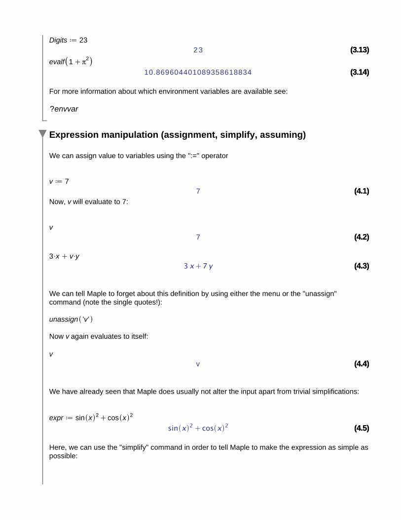
Related to "eval" is the command "evalf" ("evaluate to a floating point number:)

10.86960440

We can control the accuracy by either supplying this information in brackets

10.869604401089358619

or by setting the system variable "Digits":

(4.2)(4.2)

(4.3)(4.3)

(3.13)(3.13)

(3.14)(3.14)

(4.1)(4.1)

(2.13)(2.13)

(1.17)(1.17)

(4.5)(4.5)

(4.4)(4.4)

2 3

10.869604401089358618834

For more information about which environment variables are available see:

Expression manipulation (assignment, simplify, assuming)

We can assign value to variables using the ":=" operator

7

Now, will evaluate to 7:

7

We can tell Maple to forget about this definition by using either the menu or the "unassign" command (note the single quotes!):

Now again evaluates to itself:

v

We have already seen that Maple does usually not alter the input apart from trivial simplifications:

Here, we can use the "simplify" command in order to tell Maple to make the expression as simple aspossible:

(4.6)(4.6)

(4.10)(4.10)

(4.9)(4.9)

(4.7)(4.7)

(2.13)(2.13)

(1.17)(1.17)

(4.8)(4.8)

1

Sometimes, expressions don't get fully simplified:

Maple can't do any simplification here, because it does not have enough information on the variables. We can supply more information using the "assuming" statement:

We can also put global assumptions on variables using the "assume" command:

(Maple marks the presence of assumptions by a tilde - this can be changed using the "ToolsOptions" menu.)

We can remove the assumptions with "unassign"

Now, again

Alternatively, we can also restart the Maple session. This will remove all assigments which we have made. To restart either type

or use the corresponding icon.

FunctionsWe can assign (mathematical) functions in Maple using an "arrow notation" (type "-" and ">"):

(5.3)(5.3)

(5.2)(5.2)

(5.6)(5.6)

(5.4)(5.4)

(5.11)(5.11)

(2.13)(2.13)

(5.10)(5.10)

(5.9)(5.9)

(5.5)(5.5)

(5.8)(5.8)

(5.1)(5.1)

(1.17)(1.17)

(5.7)(5.7)

We can now compute different values of by using the normal function notation:

0

0

For functions of more than one argument, we have to enclose the arguments in brackets:

The application of uses again the normal mathematical notation:

Note, that the following statement does not define a function in older versions of Maple (or the command line version of Maple):

(Modern versions will define a function here and some versions of Maple will ask us whether we actually meant to define a function.)

If we choose "remember table assigment" (the default in older versions), then this will not make a function.

(5.13)(5.13)

(5.14)(5.14)

(2.13)(2.13)

(5.16)(5.16)

(5.1)(5.1)

(1.17)(1.17)

(5.12)(5.12)

(5.15)(5.15)

(5.18)(5.18)

(5.17)(5.17)

Only when applied to will we see the definition

Another way of obtaining a function is to start from an expression and then to declare some of the variables as parameters using the "unapply" command:

We can define piecewise functions using either the "piecewise" command

1 3

7

See also the plot of (open the context menu by right clicking and then choose "Plots 2-D Plot"):

(2.13)(2.13)

(5.1)(5.1)

(1.17)(1.17)

(5.19)(5.19)

Or we can use the expressions palette

See also the plot for :

(6.2)(6.2)

(6.1)(6.1)

(2.13)(2.13)

(5.1)(5.1)

(1.17)(1.17)

SetsMaple can compute with (finite) sets.

We can define sets by enclosing the objects in curly braces:

As expected, sets contain each element only once:

Maple does know the usual set operations: Intersection

(6.5)(6.5)

(6.3)(6.3)

(2.13)(2.13)

(6.7)(6.7)

(6.10)(6.10)

(6.6)(6.6)

(6.8)(6.8)

(6.4)(6.4)

(6.11)(6.11)

(6.12)(6.12)

(5.1)(5.1)

(1.17)(1.17)

(6.9)(6.9)

(use the palette for the last input or type "cap [Esc]").

We can do unions:

(use the palette or type "cup [Esc]").

And differences

(use the palette or type "bsol [Esc]").

We can compute the cardinality of a set with the "numelems" function:

3

We can also compute relations between sets:

false

true

false

Finally, we can also test for membership:

(6.3)(6.3)

(7.2)(7.2)

(2.13)(2.13)

(6.13)(6.13)

(7.1)(7.1)

(7.6)(7.6)

(7.5)(7.5)

(6.15)(6.15)

(7.3)(7.3)

(7.4)(7.4)

(6.14)(6.14)

(5.1)(5.1)

(1.17)(1.17)

Here, Maple does not evaluate the statement to a truth value. We have to use the "evalb" command ("evaluate to a boolean value"):

true

false

Derivation and integration

Maple can compute derivatives of symbolic expressions using the "diff" command:

1

Recent versions of Maple also recognise the "prime" notation to mean derivation with respect to :

differentiate w.r.t. x

(also the right click context menu can be used.)

Here, the first argument is the expression and the second argument is the variable with respect to which we derive.

x

0

We can compute partial and higher order derviatives by adding more variables as arguments:

(7.15)(7.15)

(7.10)(7.10)

(6.3)(6.3)

(7.7)(7.7)

(7.9)(7.9)

(2.13)(2.13)

(7.14)(7.14)

(7.8)(7.8)

(7.13)(7.13)

(7.16)(7.16)

(7.12)(7.12)

(7.11)(7.11)

(5.1)(5.1)

(1.17)(1.17)

(7.17)(7.17)

6

There is a short hand notation for multiple repetitions of the same variable using "$": The expression"x$n" refers to "n" repetitions of "x". For instance, in order to compute the 99-th derivative of , we can use:

For functions, the "D" operator is used instead of "diff":

As you can see, the result of " " is again a function.

Note, that we did not have to specify the parameter for the derivation here. It will always be the parameter of the function.

We can compute partial and iterated derivates by adding the position of the argument with respect towhich we want to derive in square brackets just after the D:

(6.3)(6.3)

(7.22)(7.22)

(2.13)(2.13)

(7.20)(7.20)

(7.18)(7.18)

(7.23)(7.23)

(7.24)(7.24)

(7.19)(7.19)

(7.25)(7.25)

(5.1)(5.1)

(1.17)(1.17)

(7.21)(7.21)

(The examples compute , , and , respectively).

It is also possible to compute higher derivatives with the "function exponentiation" operator "@@". We will discuss it in more detail later.

Antiderivatives ("indefinite integrals") can be computed using "int":

We can also use "int [Esc]" or the palettes to enter integrals:

We can compute definite integrals with the following syntax:

91 0

(6.3)(6.3)

(2.13)(2.13)

(7.27)(7.27)

(8.1)(8.1)

(8.2)(8.2)

(7.26)(7.26)

(8.4)(8.4)

(8.3)(8.3)

(5.1)(5.1)

(1.17)(1.17)

(8.5)(8.5)

1

Maple uses the two-dot ".." notation to denotes ranges of numbers.

This also works with multiple integrals.

1 31 2

Maple's integration routine supports a lot of options like, eg, numerical intgration, handling discontinuities, series expansion. See the help page for details and examples:

Sums

As we have seen in the first lecture, Maple can evaluate sums:

2

ex

The syntax is similar to integration.

If we do not give a range for the summation variable, then Maple computes an "antidifference":

(We will (probably) discuss antidifferences in the third part of the lecture when we learn how Maple actually finds these expressions.)

(9.5)(9.5)

(8.6)(8.6)

(6.3)(6.3)

(2.13)(2.13)

(9.3)(9.3)

(9.2)(9.2)

(9.1)(9.1)

(5.1)(5.1)

(1.17)(1.17)

(9.4)(9.4)

(9.6)(9.6)

There is a related command "add", which also performs a summation. However, it can only be applied to finite sums.

5 5

E r r o r , u n a b l e t o e x e c u t e a d d

We will revisit "add" when we discuss programming in Maple.

Equations

We can input equations as symbolic values in Maple

Without further instruction, Maple does not try to simplify or solve the equations.

Equations may be assigned to a variable:

(Use the underscore "_" or square brackets "[" and "]" to input indices)

We can add equations together or multiply them by values:

(10.3)(10.3)

(6.3)(6.3)

(9.9)(9.9)

(2.13)(2.13)

(9.7)(9.7)

(9.8)(9.8)

(10.1)(10.1)

(9.11)(9.11)

(9.12)(9.12)

(5.1)(5.1)

(1.17)(1.17)

(10.2)(10.2)

(9.10)(9.10)

We can access the left hand side of an equations or the right hand side of an equation with "lhs" or "rhs", respectively.

We will discuss how Maple can solve equations automatically later in this lecture.

It is also possible to enter and compute with inequalities:

(Here, the "%%" symbol refers to the second-last expression which was evaluated. There is also "%%%" for the third last expression. Use them with the same care as "%"!)

To enter and type "< =" and "> =". For type "! =".

printing, quoting, LaTeX, inert forms

Maple has a builtin command "print" which can be used to print any Maple expression:

This is not extremely useful right now, but we can make use of it later, when we write our own procedures in Maple.

Sometimes, we would like to stop Maple from evaluating a variable before printing.

(10.6)(10.6)

(10.5)(10.5)

(6.3)(6.3)

(2.13)(2.13)

(9.7)(9.7)

(10.4)(10.4)

(5.1)(5.1)

(1.17)(1.17)

For this, we can use "quotes": If we enter single quotation marks around a variable, this tells Maple not to evaluate it:

E r r o r , ( i n u n a s s i g n ) c a n n o t u n a s s i g n ` a l p h a + b e t a ^ 2 ' ( a r g u m e n t mus t be ass ignab le )

then Maple first evaluates to before applying the "unassign" command. The result is an error. If we use quotes,

then Maple does not evaluate and "unassign" is passed the just the variable .)

We can ask Maple to print an expression using LaTeX syntax:

1 / 2 \ , \ s i n \ l e f t ( x \ r i g h t )

(Maple's LaTeX output is not necessarily the most pretty one, and Maple's insistence on evaluating expressions can be annoying...)

Actually, we can enter inert (meaning unevaluated) integral using the "Int" command (notice the capitalisation!). Still Maple will not leave our expression completely untouched:

\ i n t \ ! 1 / 2 \ , \ c o s \ l e f t ( x \ r i g h t ) { d x }

Also the derivation and sum have an inert form: Use "Diff" and "Sum" (notice the capitalisation).

(10.8)(10.8)

(6.3)(6.3)

(2.13)(2.13)

(9.7)(9.7)

(10.7)(10.7)

(5.1)(5.1)

(1.17)(1.17)

On the other hand, the lowercase "sum", for instance, immeadiately evaluates it's argument:

12403