84
Basic Biostatistics Prof Paul Rheeder Division of Clinical Epidemiology
| Date post: | 02-Jan-2016 |
| Category: |
Documents |
| Upload: | lisa-summers |
| View: | 229 times |
| Download: | 4 times |

Basic Biostatistics
Prof Paul Rheeder
Division of Clinical Epidemiology


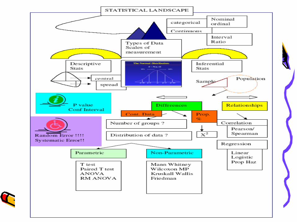
Overview• Bias vs chance• Types of data• Descriptive statistics• Histograms and boxplots• Inferential statistics• Hypothesis testing: P and CI• Comparing groups• Correlation and regression


Research Questions?• Does CK level predict in hospital
mortality post MI?• Is there an association between
troponin I and renal function?• What is the Incidence of
amputation in diabetics with renal failure?
HOW ARE THEY MEASURED???

Research question• Does aspirin reduce CV mortality
in diabetics when used for primary prevention?
• Is there an increased risk between cell phone use and brain cancer?
• Does level of SES correlate with depression?

Research question• So your research question must be
phrased in such a manner that you can answer YES or NO or provide some quantification of sorts.

Data analysis• Aim: to provide information on the
study sample and to answer the research question !

Problems !

Problems• Bias and confounding also called
systematic error…. Typically dealt with in the planning and execution of the study…can also control for it in the data analysis (eg multivariate analysis)
• Chance also called random error. Classically P values (and CI) can be used to judge role of chance

First important issues• What type of data are you collecting
• Typically one has some outcome variable and some exposure variable or variables?
• How and with what are they measured?
Outcome and exposure?
• Does CK level predict in hospital mortality post MI?
• Is there an association between troponin I and renal function?
• What is the Incidence of amputation in diabetics with renal failure?
HOW ARE THEY MEASURED???

Research question• Does aspirin reduce CV mortality
in diabetics when used for primary prevention?
• Is there an increased risk between cell phone use and brain cancer?
• Does level of SES correlate with depression?

Research question• So your research question must be
phrased in such a manner that you can answer YES or NO or provide some quantification of sorts.

Types of data• Categorical: HT yes or no, sex,
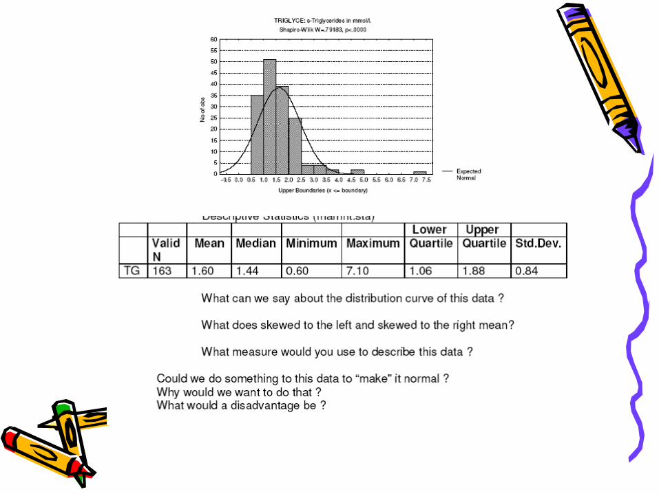
smoking status (usually a %)• Ordinal versus nominal• Continuous data• Spread of continuous data

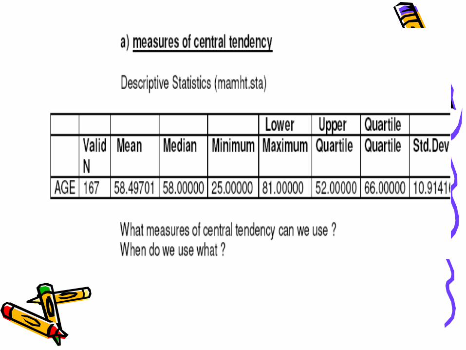
Data analysis• Descriptive stats
• Mean/median
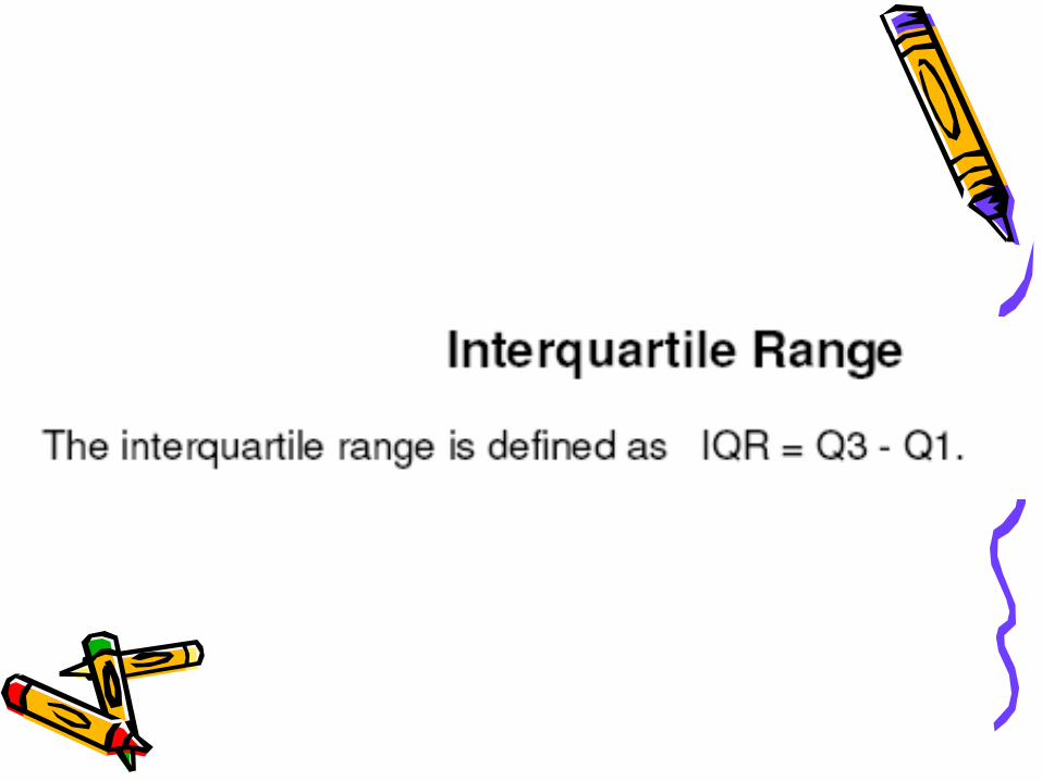
• SD or range

Hypothesis testing• Differences between groups:• Examples:• T test/Mann Whitney (2 groups)• ANOVA/ Kruskal Wallis (>2 groups)• Chi square if it is %

• Associations between variables• Does coffee cause cancer (OR, RR)• Efficacy of Rx (RRR, ARR, NNT)• If BMI associated with BP
(correlation and regression)

2 X 2 tableCancer No cancer
Smoke a b
Non smoker c d
RR= (a/a+b)/(c/c+d) OR = (a/b)/(c/d)


TYPES OF DATA
DESCRIPTIVE STATS


Graphics
40
50
60
70
ag
e in
ye
ars
1 2 3


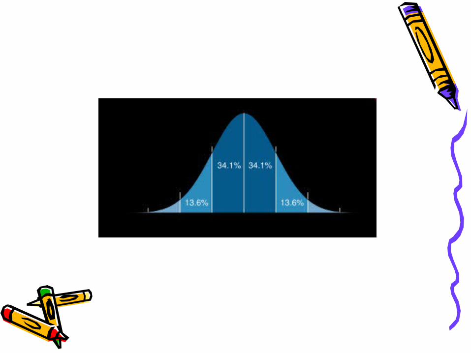
Using the SD and the Normal Curve


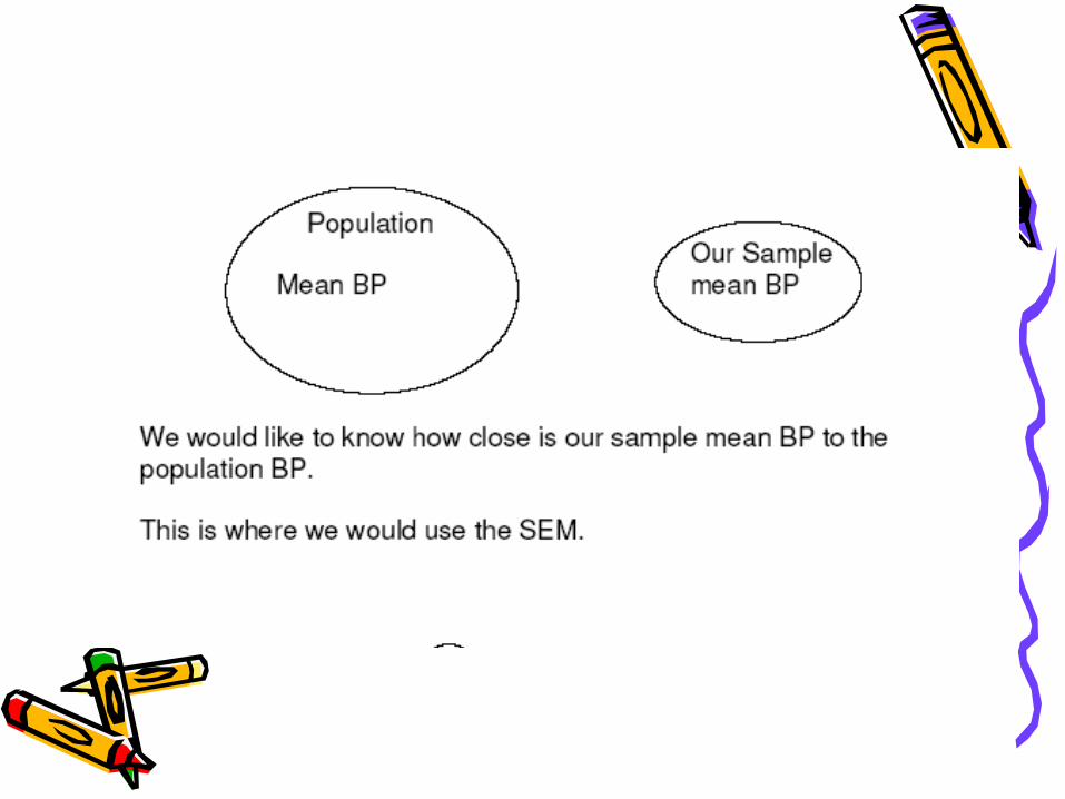
• Mean ± 1.96 SD = 95% range of sample
• Mean ± 1.96 SEM=95% Confidence interval

One of many samples


95% Confidence Intervals


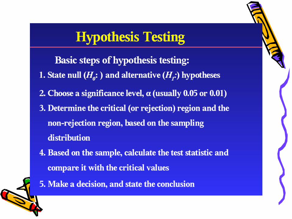
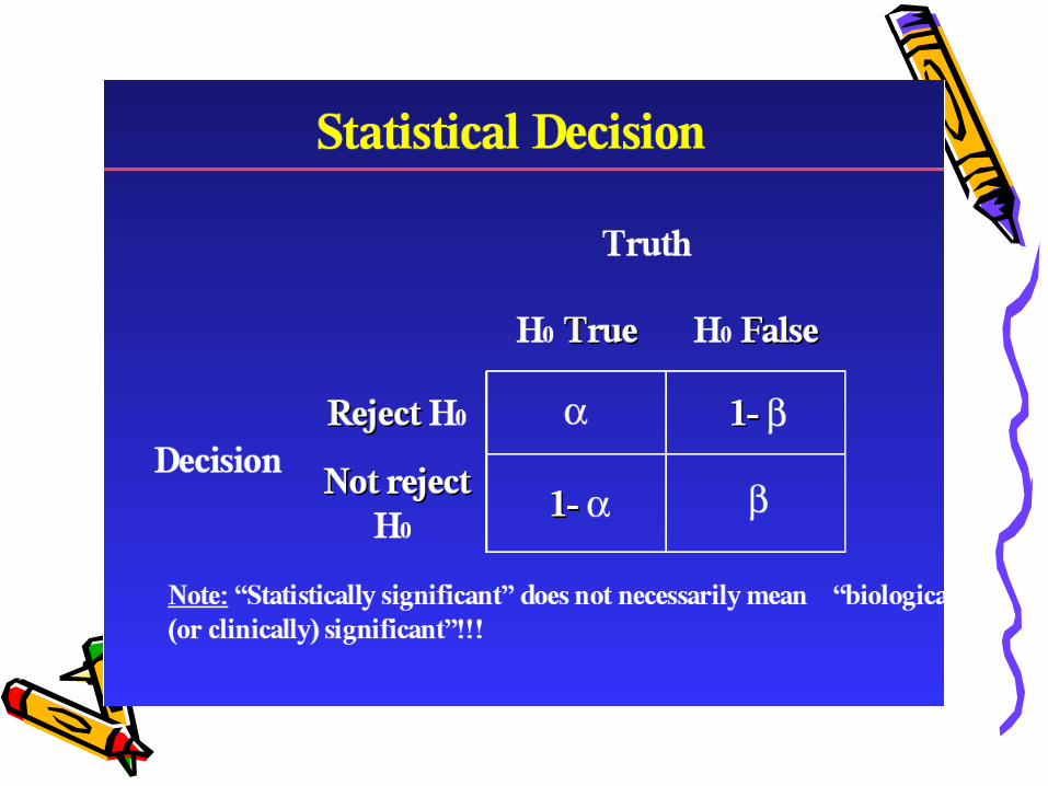
Hypothesis Testing


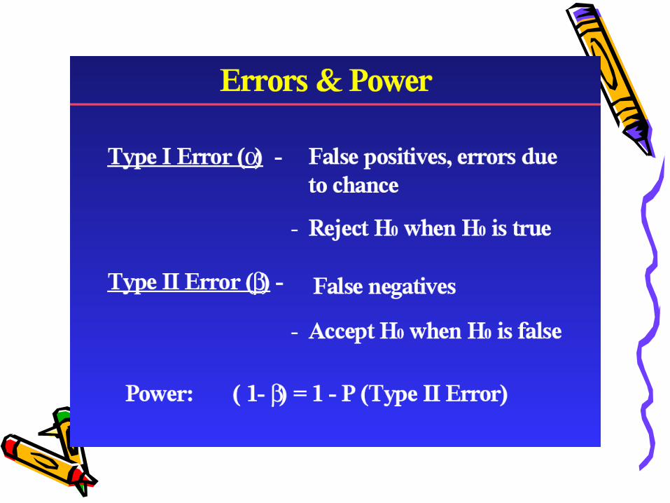


Type I & II Errors Have an Inverse Relationship
If you reduce the probability of one error, the other one increases so that everything else is unchanged.
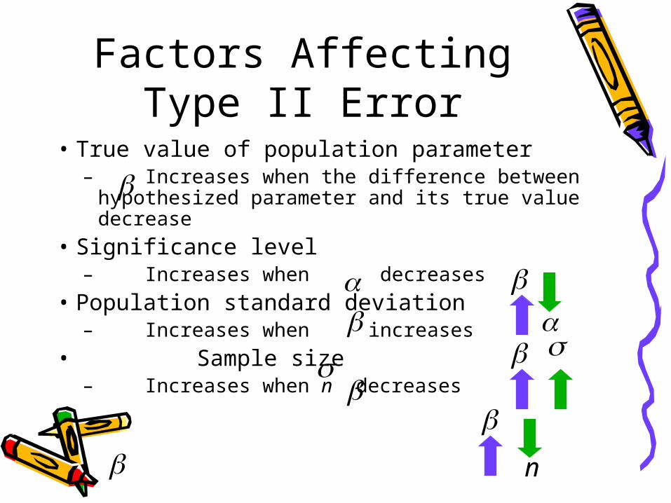
Factors Affecting Type II Error
• True value of population parameter– Increases when the difference between
hypothesized parameter and its true value decrease
• Significance level– Increases when decreases
• Population standard deviation– Increases when increases
• Sample size– Increases when n decreases
n

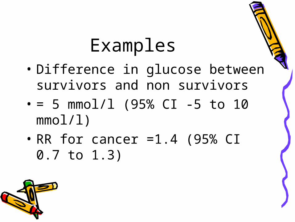
Examples• Difference in glucose between
survivors and non survivors• = 5 mmol/l (95% CI -5 to 10
mmol/l)• RR for cancer =1.4 (95% CI 0.7 to
1.3)


P value• The H0 is NO difference• BUT I can find a difference by chance• Eg WHAT is the probability that you can
find a difference between groups of 5 mmol/l when in TRUTH the difference is ZERO?
• P=0.10

+-------------------+| Key ||-------------------|| frequency || column percentage |+-------------------+
| 0=L E=1 Y/NR | 0 1 | Total-----------+----------------------+---------- N | 28 20 | 48 | 53.85 44.44 | 49.48 -----------+----------------------+---------- Y | 24 25 | 49 | 46.15 55.56 | 50.52 -----------+----------------------+---------- Total | 52 45 | 97 | 100.00 100.00 | 100.00
Pearson chi2(1) = 0.8530 Pr = 0.356

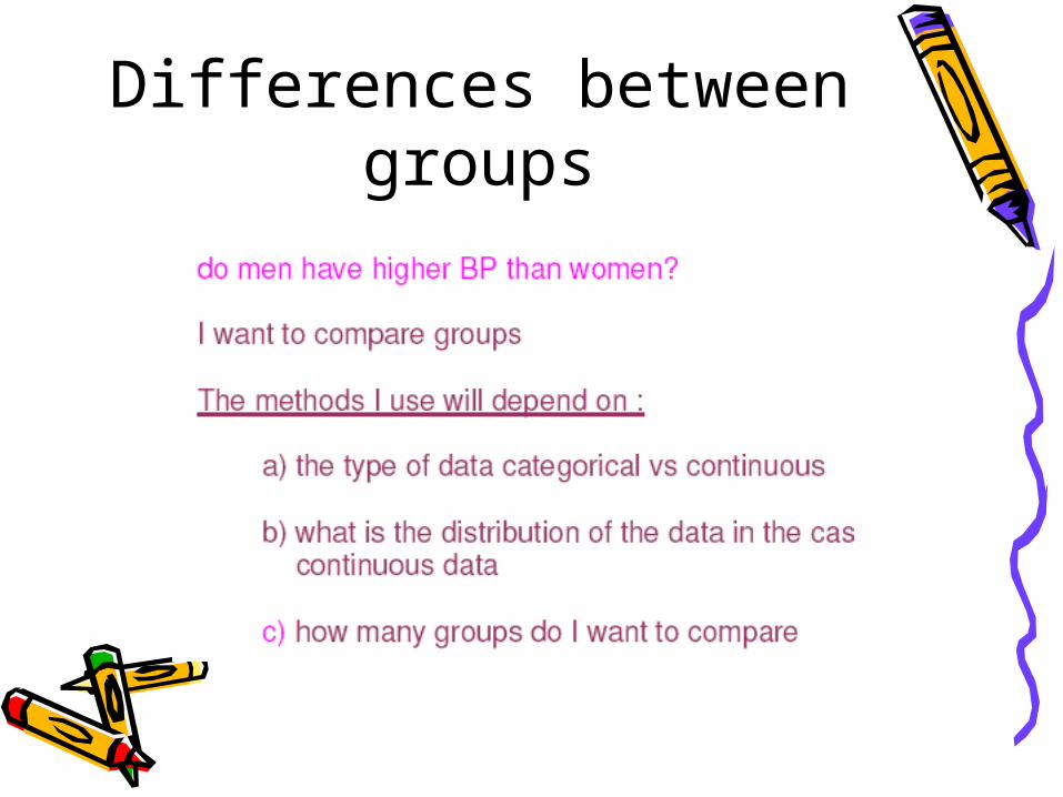
Differences between groups
Parametric comparisons

?
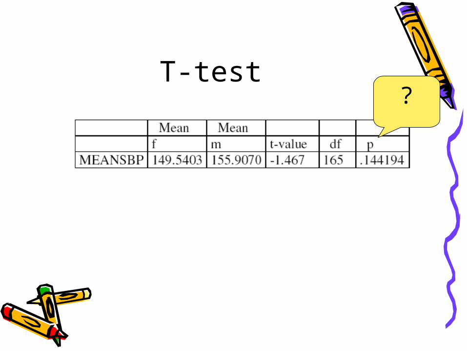
T-test?
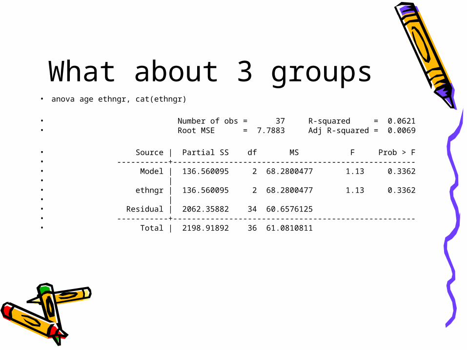
What about 3 groups• anova age ethngr, cat(ethngr)
• Number of obs = 37 R-squared = 0.0621• Root MSE = 7.7883 Adj R-squared = 0.0069
• Source | Partial SS df MS F Prob > F• -----------+----------------------------------------------------• Model | 136.560095 2 68.2800477 1.13 0.3362• |• ethngr | 136.560095 2 68.2800477 1.13 0.3362• |• Residual | 2062.35882 34 60.6576125 • -----------+----------------------------------------------------• Total | 2198.91892 36 61.0810811
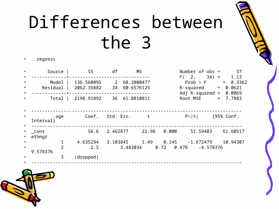
Differences between the 3
• . regress
• Source | SS df MS Number of obs = 37• -------------+------------------------------ F( 2, 34) = 1.13• Model | 136.560095 2 68.2800477 Prob > F = 0.3362• Residual | 2062.35882 34 60.6576125 R-squared = 0.0621• -------------+------------------------------ Adj R-squared = 0.0069• Total | 2198.91892 36 61.0810811 Root MSE = 7.7883
• ------------------------------------------------------------------------------• age Coef. Std. Err. t P>|t| [95% Conf. Interval] • ------------------------------------------------------------------------------• _cons 56.6 2.462877 22.98 0.000 51.59483 61.60517• ethngr• 1 4.635294 3.103845 1.49 0.145 -1.672479 10.94307• 2 2.5 3.483034 0.72 0.478 -4.578376 9.578376• 3 (dropped)• ------------------------------------------------------------------------------

Repeated measures• One group of schoolkids• Muscle strength in January• Muscle strength again in March• Did things change significantly over
time?• Paired T –test• Two or more groups: RM ANOVA
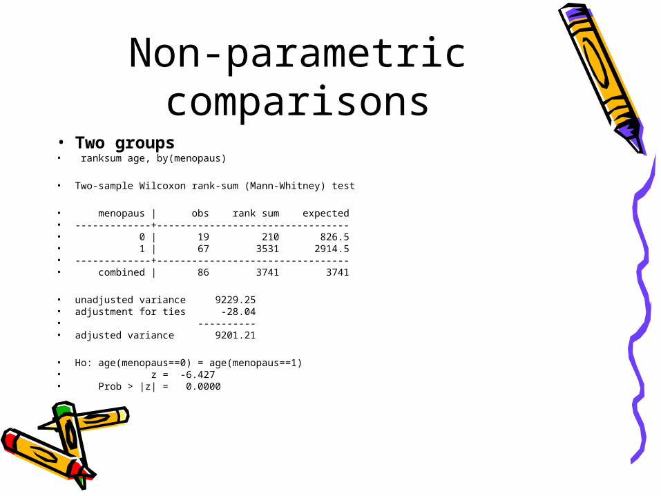
Non-parametric comparisons
• Two groups• ranksum age, by(menopaus)
• Two-sample Wilcoxon rank-sum (Mann-Whitney) test
• menopaus | obs rank sum expected• -------------+---------------------------------• 0 | 19 210 826.5• 1 | 67 3531 2914.5• -------------+---------------------------------• combined | 86 3741 3741
• unadjusted variance 9229.25• adjustment for ties -28.04• ----------• adjusted variance 9201.21
• Ho: age(menopaus==0) = age(menopaus==1)• z = -6.427• Prob > |z| = 0.0000
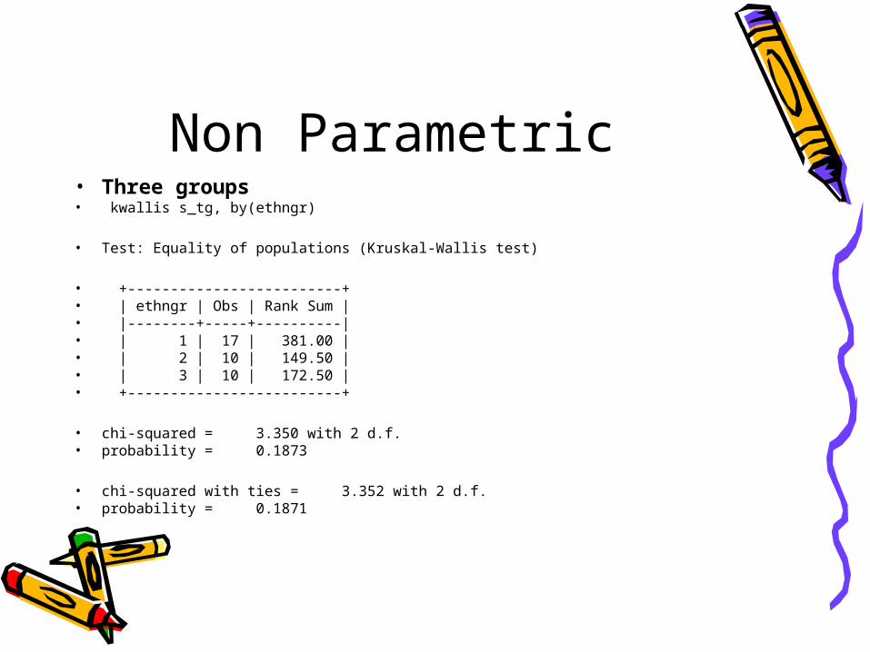
Non Parametric• Three groups• kwallis s_tg, by(ethngr)
• Test: Equality of populations (Kruskal-Wallis test)
• +-------------------------+• | ethngr | Obs | Rank Sum |• |--------+-----+----------|• | 1 | 17 | 381.00 |• | 2 | 10 | 149.50 |• | 3 | 10 | 172.50 |• +-------------------------+
• chi-squared = 3.350 with 2 d.f.• probability = 0.1873
• chi-squared with ties = 3.352 with 2 d.f.• probability = 0.1871

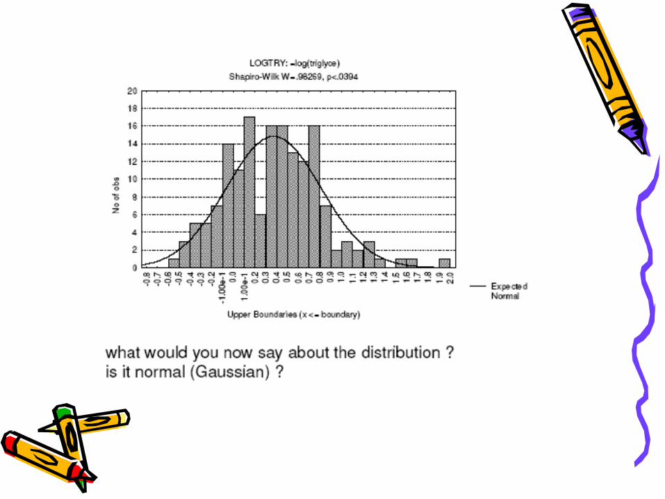
summarize• Continuous-Non Normal• 2 groups: Mann Whitney• 3 groups: Kruskal Wallis
• Continuous-Normal• 2 groups: T tests• 3 groups: ANOVA

Categorical data

Relationships


Linear Regression
• Here the DEPENDENT (logTG) and INDEPENDENT VARIABLES are continuous
• So how much does logTG increase if waist increases by 1cm = the beta coefficient
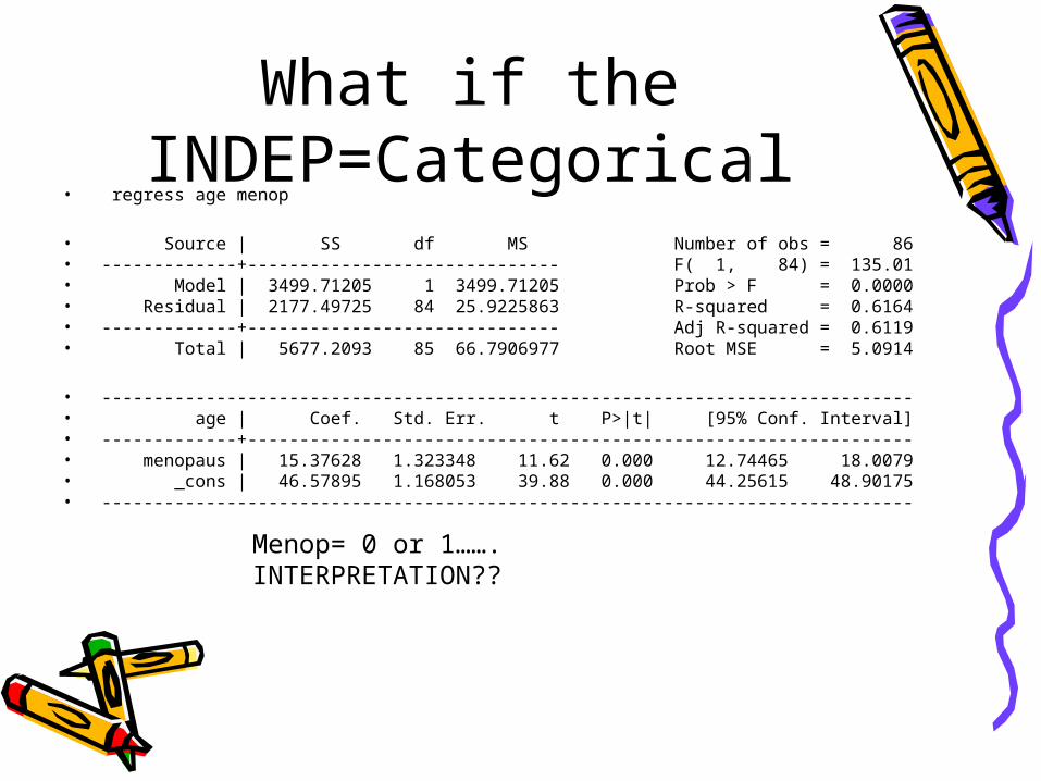
What if the INDEP=Categorical
• regress age menop
• Source | SS df MS Number of obs = 86• -------------+------------------------------ F( 1, 84) = 135.01• Model | 3499.71205 1 3499.71205 Prob > F = 0.0000• Residual | 2177.49725 84 25.9225863 R-squared = 0.6164• -------------+------------------------------ Adj R-squared = 0.6119• Total | 5677.2093 85 66.7906977 Root MSE = 5.0914
• ------------------------------------------------------------------------------• age | Coef. Std. Err. t P>|t| [95% Conf. Interval]• -------------+----------------------------------------------------------------• menopaus | 15.37628 1.323348 11.62 0.000 12.74465 18.0079• _cons | 46.57895 1.168053 39.88 0.000 44.25615 48.90175• ------------------------------------------------------------------------------
Menop= 0 or 1……. INTERPRETATION??

Logistic regression• Outcome is heart disease (Yes/No… ?)• Independent var = age• . logistic CVD age
• Logistic regression Number of obs = 48• LR chi2(1) = 2.51• Prob > chi2 = 0.1133• Log likelihood = -29.945379 Pseudo R2 = 0.0402
• died | Odds Ratio Std. Err. z P>|z| [95% Conf. Interval]• -------------+------------------------------------------------------------ age |
1.093467 .064069 1.52 0.127 .9748363 1.226535• ---------------------------------------------------------------------------
?


