75
Basic Markov Chains Pierre Br´ emaud December 9, 2015

Basic Markov Chains
Pierre Bremaud
December 9, 2015

2
Contents
1 The transition matrix 5
1.1 The distribution of a Markov chain . . . . . . . . . . . . . . . . . . . . . . . . . . 51.2 Communication and period . . . . . . . . . . . . . . . . . . . . . . . . . . . . . . 121.3 Stationarity and reversibility . . . . . . . . . . . . . . . . . . . . . . . . . . . . . 141.4 Strong Markov property . . . . . . . . . . . . . . . . . . . . . . . . . . . . . . . . 171.5 Exercises . . . . . . . . . . . . . . . . . . . . . . . . . . . . . . . . . . . . . . . . 21
2 Recurrence 23
2.1 The potential matrix criterion . . . . . . . . . . . . . . . . . . . . . . . . . . . . . 232.2 Stationary distribution criterion . . . . . . . . . . . . . . . . . . . . . . . . . . . . 272.3 Foster’s theorem . . . . . . . . . . . . . . . . . . . . . . . . . . . . . . . . . . . . 322.4 Examples . . . . . . . . . . . . . . . . . . . . . . . . . . . . . . . . . . . . . . . . 362.5 Exercises . . . . . . . . . . . . . . . . . . . . . . . . . . . . . . . . . . . . . . . . 42
3 Long-run behaviour 45
3.1 Ergodic theorem . . . . . . . . . . . . . . . . . . . . . . . . . . . . . . . . . . . . 453.2 Convergence in variation . . . . . . . . . . . . . . . . . . . . . . . . . . . . . . . . 483.3 Monte Carlo . . . . . . . . . . . . . . . . . . . . . . . . . . . . . . . . . . . . . . . 583.4 Absorption . . . . . . . . . . . . . . . . . . . . . . . . . . . . . . . . . . . . . . . 653.5 Exercises . . . . . . . . . . . . . . . . . . . . . . . . . . . . . . . . . . . . . . . . 72
4 Solutions 77
A Appendix 89
A.1 Greatest Common Divisor . . . . . . . . . . . . . . . . . . . . . . . . . . . . . . . 89A.2 Dominated convergence for series . . . . . . . . . . . . . . . . . . . . . . . . . . . 91
3

4 CONTENTS
Chapter 1
The transition matrix
1.1 The distribution of a Markov chain
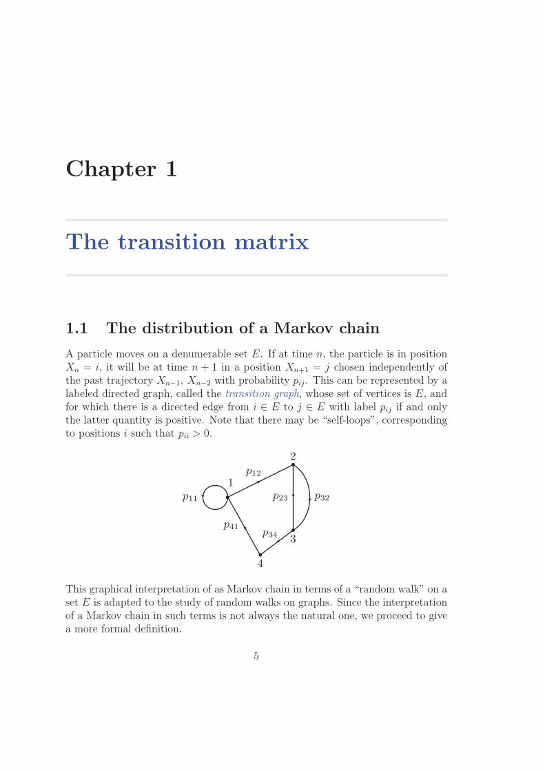
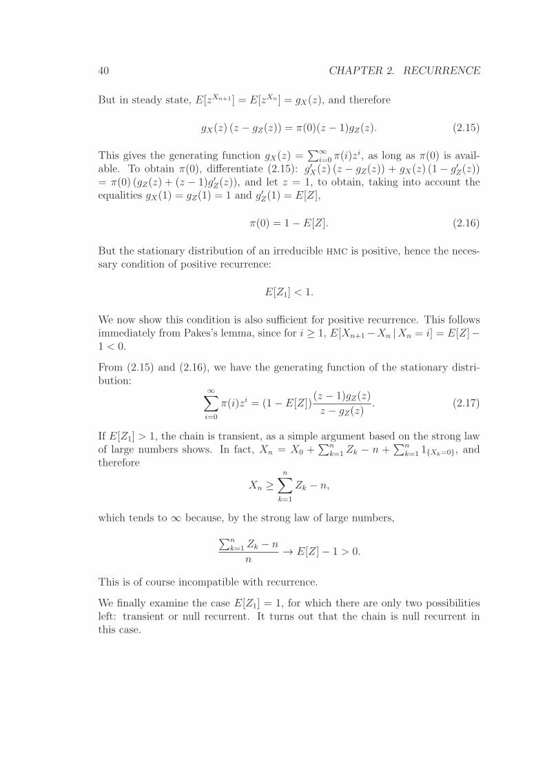
A particle moves on a denumerable set E. If at time n, the particle is in positionXn = i, it will be at time n + 1 in a position Xn+1 = j chosen independently ofthe past trajectory Xn−1, Xn−2 with probability pij. This can be represented by alabeled directed graph, called the transition graph, whose set of vertices is E, andfor which there is a directed edge from i ∈ E to j ∈ E with label pij if and onlythe latter quantity is positive. Note that there may be “self-loops”, correspondingto positions i such that pii > 0.
1
2
3
4
p12
p23
p34
p32
p41
p11
This graphical interpretation of as Markov chain in terms of a “random walk” on aset E is adapted to the study of random walks on graphs. Since the interpretationof a Markov chain in such terms is not always the natural one, we proceed to givea more formal definition.
5
6 CHAPTER 1. THE TRANSITION MATRIX
Recall that a sequence {Xn}n≥0 of random variables with values in a set E is calleda discrete-time stochastic process with state space E. In this chapter, the statespace is countable, and its elements will be denoted by i, j, k,. . . If Xn = i, theprocess is said to be in state i at time n, or to visit state i at time n.
Definition 1.1.1 If for all integers n ≥ 0 and all states i0, i1, . . . , in−1, i, j,
P (Xn+1 = j |Xn = i,Xn−1 = in−1, . . . , X0 = i0) = P (Xn+1 = j |Xn = i) ,
this stochastic process is called a Markov chain, and a homogeneous Markov chain(hmc) if, in addition, the right-hand side is independent of n.
The matrix P = {pij}i,j∈E, where
pij = P (Xn+1 = j |Xn = i),
is called the transition matrix of the hmc. Since the entries are probabilities, andsince a transition from any state i must be to some state, it follows that
pij ≥ 0, and∑
k∈E
pik = 1
for all states i, j. A matrix P indexed by E and satisfying the above properties iscalled a stochastic matrix. The state space may be infinite, and therefore such amatrix is in general not of the kind studied in linear algebra. However, the basicoperations of addition and multiplication will be defined by the same formal rules.The notation x = {x(i)}i∈E formally represents a column vector, and xT is thecorresponding row vector.
The Markov property easily extends (Exercise 1.5.2) to
P (A |Xn = i, B) = P (A |Xn = i) ,
where
A = {Xn+1 = j1, . . . , Xn+k = jk}, B = {X0 = i0, . . . , Xn−1 = in−1}.
This is in turn equivalent to
P (A ∩ B |Xn = i) = P (A |Xn = i)P (B |Xn = i).
That is, A and B are conditionaly independent given Xn = i. In other words, thefuture at time n and the past at time n are conditionally independent given the
1.1. THE DISTRIBUTION OF A MARKOV CHAIN 7
present state Xn = i. In particular, the Markov property is independent of thedirection of time.
Notation. We shall from now on abbreviate P (A |X0 = i) as Pi(A). Also, if µ isa probability distribution on E, then Pµ(A) is the probability of A given that theinitial state X0 is distributed according to µ.
The distribution at time n of the chain is the vector νn := {νn(i)}i∈E, where
νn(i) := P (Xn = i).
From the Bayes rule of exclusive and exhaustive causes, νn+1(j) =∑
i∈E νn(i)pij,that is, in matrix form, νTn+1 = νTnP. Iteration of this equality yields
νTn = νT0 Pn. (1.1)
The matrix Pm is called the m-step transition matrix because its general term is
pij(m) = P (Xn+m = j |Xn = i).
In fact, by the Bayes sequential rule and the Markov property, the right-hand sideequals
∑i1,...,im−1∈E
pii1pi1i2 · · · pim−1j, which is the general term of the m-th powerof P.
The probability distribution ν0 of the initial state X0 is called the initial distri-bution. From the Bayes sequential rule and in view of the homogeneous Markovproperty and the definition of the transition matrix,
P (X0 = i0, X1 = i1, . . . , Xk = ik) = ν0(i0)pi0i1 · · · pik−1ik .
Therefore,
Theorem 1.1.1 The distribution of a discrete-time hmc is uniquely determinedby its initial distribution and its transition matrix.
Sample path realization
Many hmc’s receive a natural description in terms of a recurrence equation.
Theorem 1.1.2 Let {Zn}n≥1 be an iid sequence of random variables with valuesin an arbitrary space F . Let E be a countable space, and f : E × F → E be somefunction. Let X0 be a random variable with values in E, independent of {Zn}n≥1.The recurrence equation
Xn+1 = f(Xn, Zn+1) (1.2)
then defines a hmc.
8 CHAPTER 1. THE TRANSITION MATRIX
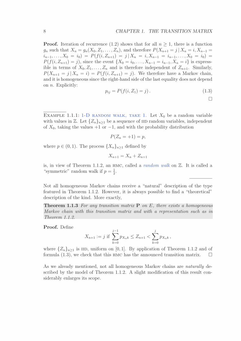
Proof. Iteration of recurrence (1.2) shows that for all n ≥ 1, there is a functiongn such that Xn = gn(X0, Z1, . . . , Zn), and therefore P (Xn+1 = j |Xn = i,Xn−1 =in−1, . . . , X0 = i0) = P (f(i, Zn+1) = j |Xn = i,Xn−1 = in−1, . . . , X0 = i0) =P (f(i, Zn+1) = j), since the event {X0 = i0, . . . , Xn−1 = in−1, Xn = i} is express-ible in terms of X0, Z1, . . . , Zn and is therefore independent of Zn+1. Similarly,P (Xn+1 = j |Xn = i) = P (f(i, Zn+1) = j). We therefore have a Markov chain,and it is homogeneous since the right-hand side of the last equality does not dependon n. Explicitly:
pij = P (f(i, Z1) = j) . (1.3)
�
Example 1.1.1: 1-D random walk, take 1. Let X0 be a random variablewith values in Z. Let {Zn}n≥1 be a sequence of iid random variables, independentof X0, taking the values +1 or −1, and with the probability distribution
P (Zn = +1) = p,
where p ∈ (0, 1). The process {Xn}n≥1 defined by
Xn+1 = Xn + Zn+1
is, in view of Theorem 1.1.2, an hmc, called a random walk on Z. It is called a“symmetric” random walk if p = 1
2.
Not all homogeneous Markov chains receive a “natural” description of the typefeatured in Theorem 1.1.2. However, it is always possible to find a “theoretical”description of the kind. More exactly,
Theorem 1.1.3 For any transition matrix P on E, there exists a homogeneousMarkov chain with this transition matrix and with a representation such as inTheorem 1.1.2.
Proof. Define
Xn+1 := j if
j−1∑
k=0
pXnk ≤ Zn+1 <
j∑
k=0
pXnk ,
where {Zn}n≥1 is iid, uniform on [0, 1]. By application of Theorem 1.1.2 and offormula (1.3), we check that this hmc has the announced transition matrix. �
As we already mentioned, not all homogeneous Markov chains are naturally de-scribed by the model of Theorem 1.1.2. A slight modification of this result con-siderably enlarges its scope.
1.1. THE DISTRIBUTION OF A MARKOV CHAIN 9
Theorem 1.1.4 Let things be as in Theorem 1.1.2 except for the joint distribu-tion of X0, Z1, Z2, . . .. Suppose instead that for all n ≥ 0, Zn+1 is condition-ally independent of Zn, . . . , Z1, Xn−1, . . . , X0 given Xn, and that for all i, j ∈ E,P (Zn+1 = k |Xn = i) is independent of n. Then {Xn}n≥0 is a hmc, with transitionprobabilities
pij = P (f(i, Z1) = j |X0 = i).
Proof. The proof is quite similar to that of Theorem 1.1.2 (Exercise ??). �
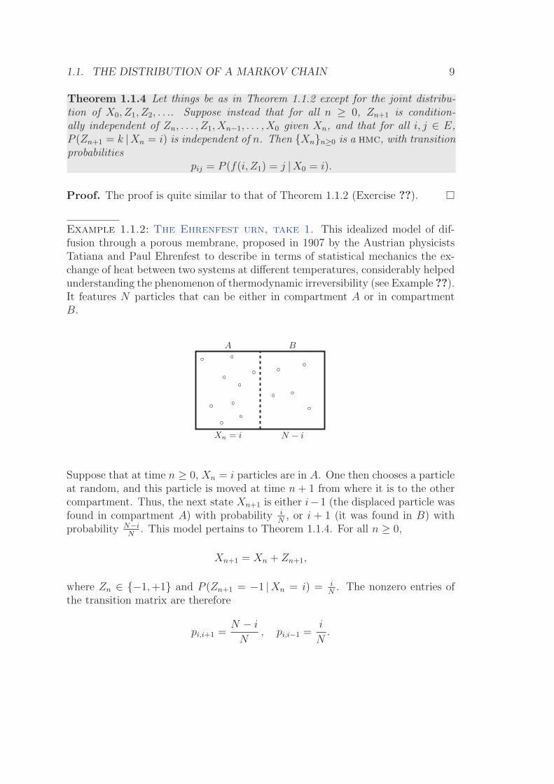
Example 1.1.2: The Ehrenfest urn, take 1. This idealized model of dif-fusion through a porous membrane, proposed in 1907 by the Austrian physicistsTatiana and Paul Ehrenfest to describe in terms of statistical mechanics the ex-change of heat between two systems at different temperatures, considerably helpedunderstanding the phenomenon of thermodynamic irreversibility (see Example ??).It features N particles that can be either in compartment A or in compartmentB.
A B
Xn = i N − i
Suppose that at time n ≥ 0, Xn = i particles are in A. One then chooses a particleat random, and this particle is moved at time n + 1 from where it is to the othercompartment. Thus, the next state Xn+1 is either i−1 (the displaced particle wasfound in compartment A) with probability i
N, or i + 1 (it was found in B) with
probability N−iN
. This model pertains to Theorem 1.1.4. For all n ≥ 0,
Xn+1 = Xn + Zn+1,
where Zn ∈ {−1,+1} and P (Zn+1 = −1 |Xn = i) = iN. The nonzero entries of
the transition matrix are therefore
pi,i+1 =N − i
N, pi,i−1 =
i
N.
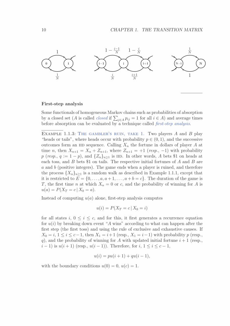
10 CHAPTER 1. THE TRANSITION MATRIX
1 1−i−1
N1−
i
N
1
N
1
N
i
N
i+1
N1
0 1 i−1 i i+1 N−1 N
First-step analysis
Some functionals of homogeneous Markov chains such as probabilities of absorptionby a closed set (A is called closed if
∑j∈A pij = 1 for all i ∈ A) and average times
before absorption can be evaluated by a technique called first-step analysis.
Example 1.1.3: The gambler’s ruin, take 1. Two players A and B play“heads or tails”, where heads occur with probability p ∈ (0, 1), and the successiveoutcomes form an iid sequence. Calling Xn the fortune in dollars of player A attime n, then Xn+1 = Xn + Zn+1, where Zn+1 = +1 (resp., −1) with probabilityp (resp., q := 1 − p), and {Zn}n≥1 is iid. In other words, A bets $1 on heads ateach toss, and B bets $1 on tails. The respective initial fortunes of A and B area and b (positive integers). The game ends when a player is ruined, and thereforethe process {Xn}n≥1 is a random walk as described in Example 1.1.1, except thatit is restricted to E = {0, . . . , a, a+1, . . . , a+ b = c}. The duration of the game isT , the first time n at which Xn = 0 or c, and the probability of winning for A isu(a) = P (XT = c |X0 = a).
Instead of computing u(a) alone, first-step analysis computes
u(i) = P (XT = c |X0 = i)
for all states i, 0 ≤ i ≤ c, and for this, it first generates a recurrence equationfor u(i) by breaking down event “A wins” according to what can happen after thefirst step (the first toss) and using the rule of exclusive and exhaustive causes. IfX0 = i, 1 ≤ i ≤ c−1, then X1 = i+1 (resp., X1 = i−1) with probability p (resp.,q), and the probability of winning for A with updated initial fortune i+ 1 (resp.,i− 1) is u(i+ 1) (resp., u(i− 1)). Therefore, for i, 1 ≤ i ≤ c− 1,
u(i) = pu(i+ 1) + qu(i− 1),
with the boundary conditions u(0) = 0, u(c) = 1.
1.1. THE DISTRIBUTION OF A MARKOV CHAIN 11
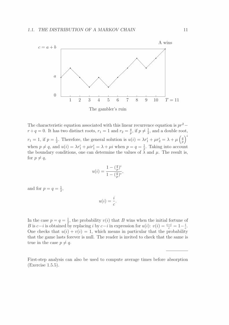
1 2 3 4 5 6 7 8 9 10 T = 11
c = a+ b
0
a
A wins
The gambler’s ruin
The characteristic equation associated with this linear recurrence equation is pr2−r+ q = 0. It has two distinct roots, r1 = 1 and r2 =
qp, if p 6= 1
2, and a double root,
r1 = 1, if p = 12. Therefore, the general solution is u(i) = λri1 + µri2 = λ + µ
(qp
)i
when p 6= q, and u(i) = λri1 + µiri1 = λ+ µi when p = q = 12. Taking into account
the boundary conditions, one can determine the values of λ and µ. The result is,for p 6= q,
u(i) =1− ( q
p)i
1− ( qp)c,
and for p = q = 12,
u(i) =i
c.
In the case p = q = 12, the probability v(i) that B wins when the initial fortune of
B is c−i is obtained by replacing i by c−i in expression for u(i): v(i) = c−ic
= 1− ic.
One checks that u(i) + v(i) = 1, which means in particular that the probabilitythat the game lasts forever is null. The reader is invited to check that the same istrue in the case p 6= q.
First-step analysis can also be used to compute average times before absorption(Exercise 1.5.5).
12 CHAPTER 1. THE TRANSITION MATRIX
1.2 Communication and period
Communication and period are topological properties in the sense that they concernonly the naked transition graph (with only the arrows, without the labels).
Communication and irreducibility
Definition 1.2.1 State j is said to be accessible from state i if there exists M ≥ 0such that pij(M) > 0. States i and j are said to communicate if i is accessiblefrom j and j is accessible from i, and this is denoted by i↔ j.
In particular, a state i is always accessible from itself, since pii(0) = 1 (P0 = I,the identity).
For M ≥ 1, pij(M) =∑
i1,...,iM−1pii1 · · · piM−1j, and therefore pij(M) > 0 if and
only if there exists at least one path i, i1, . . . , iM−1, j from i to j such that
pii1pi1i2 · · · piM−1j > 0,
or, equivalently, if there is a directed path from i to j in the transition graph G.Clearly,
i↔ i (reflexivity),
i↔ j ⇒ j ↔ i (symmetry),
i↔ j, j ↔ k ⇒ i↔ k (transivity).
Therefore, the communication relation (↔) is an equivalence relation, and it gen-erates a partition of the state space E into disjoint equivalence classes called com-munication classes.
Definition 1.2.2 A state i such that pii = 1 is called closed. More generally, aset C of states such that for all i ∈ C,
∑j∈C pij = 1 is called closed.
Definition 1.2.3 If there exists only one communication class, then the chain, itstransition matrix, and its transition graph are said to be irreducible.
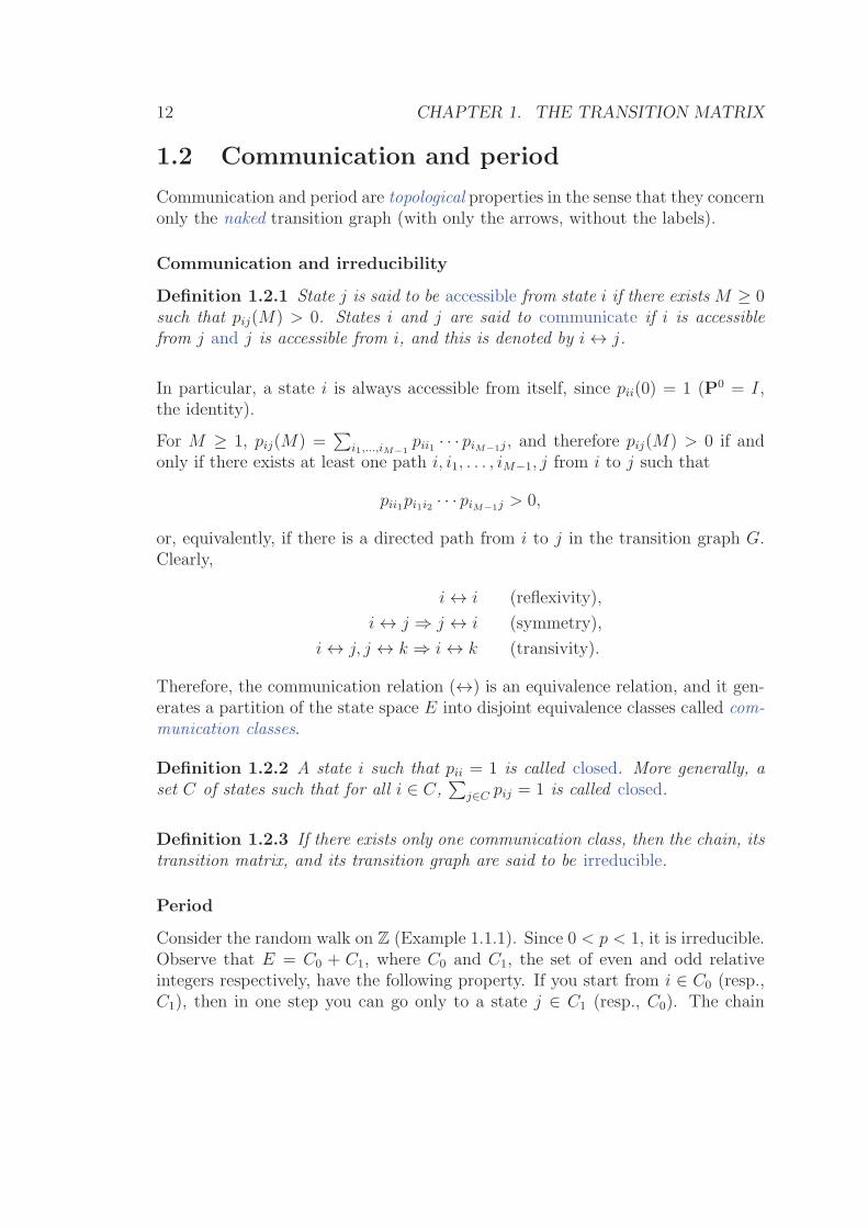
Period
Consider the random walk on Z (Example 1.1.1). Since 0 < p < 1, it is irreducible.Observe that E = C0 + C1, where C0 and C1, the set of even and odd relativeintegers respectively, have the following property. If you start from i ∈ C0 (resp.,C1), then in one step you can go only to a state j ∈ C1 (resp., C0). The chain
1.2. COMMUNICATION AND PERIOD 13
{Xn} passes alternately from cyclic class to the other. In this sense, the chainhas a periodic behavior, corresponding to the period 2. More generally, for anyirreducible Markov chain, one can find a unique partition of E into d classes C0,C1, . . ., Cd−1 such that for all k, i ∈ Ck,
∑
j∈Ck+1
pij = 1,
where by convention Cd = C0, and where d is maximal (that is, there is no othersuch partition C ′
0, C′1, . . . , C
′d′−1 with d′ > d). The proof follows directly from
Theorem 1.2.2 below.
The number d ≥ 1 is called the period of the chain (resp., of the transition ma-trix, of the transition graph). The classes C0, C1, . . . , Cd−1 are called the cyclicclasses.The chain therefore moves from one class to the other at each transition,and this cyclically.
We now give the formal definition of period. It is based on the notion of greatestcommon divisor of a set of positive integers.
Definition 1.2.4 The period di of state i ∈ E is, by definition,
di = gcd{n ≥ 1 ; pii(n) > 0},
with the convention di = +∞ if there is no n ≥ 1 with pii(n) > 0. If di = 1, thestate i is called aperiodic .
Theorem 1.2.1 If states i and j communicate they have the same period.
Proof. As i and j communicate, there exist integers N andM such that pij(M) >0 and pji(N) > 0. For any k ≥ 1,
pii(M + nk +N) ≥ pij(M)(pjj(k))npji(N)
(indeed, the path X0 = i,XM = j,XM+k = j, . . . , XM+nk = j,XM+nk+N = i isjust one way of going from i to i in M + nk +N steps). Therefore, for any k ≥ 1such that pjj(k) > 0, we have pii(M + nk + N) > 0 for all n ≥ 1. Therefore, didividesM+nk+N for all n ≥ 1, and in particular, di divides k. We have thereforeshown that di divides all k such that pjj(k) > 0, and in particular, di divides dj.By symmetry, dj divides di, and therefore, finally, di = dj. �
We can therefore speak of the period of a communication class or of an irreduciblechain.
14 CHAPTER 1. THE TRANSITION MATRIX
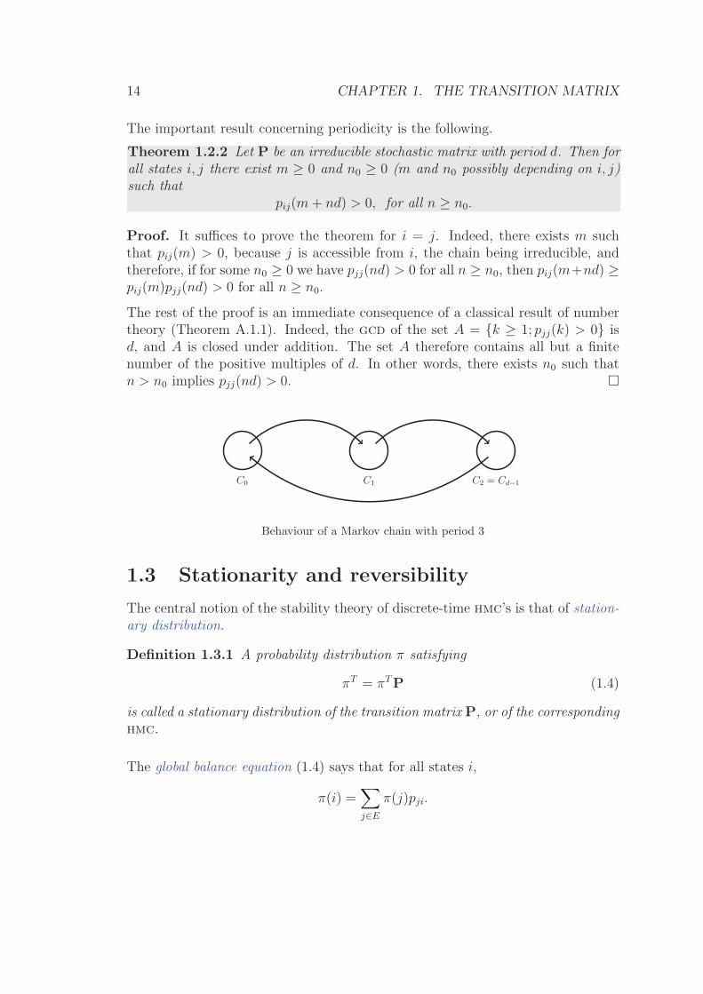
The important result concerning periodicity is the following.
Theorem 1.2.2 Let P be an irreducible stochastic matrix with period d. Then forall states i, j there exist m ≥ 0 and n0 ≥ 0 (m and n0 possibly depending on i, j)such that
pij(m+ nd) > 0, for all n ≥ n0.
Proof. It suffices to prove the theorem for i = j. Indeed, there exists m suchthat pij(m) > 0, because j is accessible from i, the chain being irreducible, andtherefore, if for some n0 ≥ 0 we have pjj(nd) > 0 for all n ≥ n0, then pij(m+nd) ≥pij(m)pjj(nd) > 0 for all n ≥ n0.
The rest of the proof is an immediate consequence of a classical result of numbertheory (Theorem A.1.1). Indeed, the gcd of the set A = {k ≥ 1; pjj(k) > 0} isd, and A is closed under addition. The set A therefore contains all but a finitenumber of the positive multiples of d. In other words, there exists n0 such thatn > n0 implies pjj(nd) > 0. �
C0 C1 C2 = Cd−1
Behaviour of a Markov chain with period 3
1.3 Stationarity and reversibility
The central notion of the stability theory of discrete-time hmc’s is that of station-ary distribution.
Definition 1.3.1 A probability distribution π satisfying
πT = πTP (1.4)
is called a stationary distribution of the transition matrix P, or of the correspondinghmc.
The global balance equation (1.4) says that for all states i,
π(i) =∑
j∈E
π(j)pji.
1.3. STATIONARITY AND REVERSIBILITY 15
Iteration of (1.4) gives πT = πTPn for all n ≥ 0, and therefore, in view of (1.1), ifthe initial distribution ν = π, then νn = π for all n ≥ 0. Thus, if a chain is startedwith a stationary distribution, it keeps the same distribution forever. But there ismore, because then,
P (Xn = i0, Xn+1 = i1, . . . , Xn+k = ik) = P (Xn = i0)pi0i1 . . . pik−1ik
= π(i0)pi0i1 . . . pik−1ik
does not depend on n. In this sense the chain is stationary. One also says that thechain is in a stationary regime, or in equilibrium, or in steady state. In summary:
Theorem 1.3.1 A hmc whose initial distribution is a stationary distribution isstationary.
The balance equation πTP = πT , together with the requirement that π be aprobability vector, that is, πT1 = 1 (where 1 is a column vector with all its entriesequal to 1), constitute when E is finite, |E|+1 equations for |E| unknown variables.One of the |E| equations in πTP = πT is superfluous given the constraint πT1 = 1.Indeed, summing up all equalities of πTP = πT yields the equality πTP1 = πT1,that is, πT1 = 1.
Example 1.3.1: Two-state Markov chain. Take E = {1, 2} and define thetransition matrix
P =
(1− α αβ 1− β
),
where α, β ∈ (0, 1). The global balance equations are
π(1) = π(1)(1− α) + π(2)β , π(2) = π(1)α + π(2)(1− β .
These two equations are dependent and reduce to the single equation π(1)α =π(2)β, to which must be added the constraint π(1) + π(2) = 1 expressing that πis a probability vector. We obtain
π(1) =β
α + β, π(2) =
α
α + β.
Example 1.3.2: The Ehrenfest urn, take 2. The global balance equationsare, for i ∈ [1, N − 1],
π(i) = π(i− 1)
(1− i− 1
N
)+ π(i+ 1)
i+ 1
N
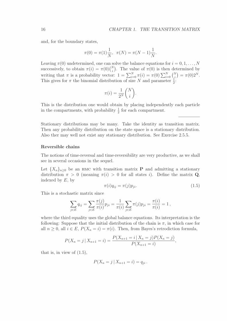
16 CHAPTER 1. THE TRANSITION MATRIX
and, for the boundary states,
π(0) = π(1)1
N, π(N) = π(N − 1)
1
N.
Leaving π(0) undetermined, one can solve the balance equations for i = 0, 1, . . . , Nsuccessively, to obtain π(i) = π(0)
(Ni
). The value of π(0) is then determined by
writing that π is a probability vector: 1 =∑N
i=0 π(i) = π(0)∑N
i=0
(Ni
)= π(0)2N .
This gives for π the binomial distribution of size N and parameter 12:
π(i) =1
2N
(N
i
).
This is the distribution one would obtain by placing independently each particlein the compartments, with probability 1
2for each compartment.
Stationary distributions may be many. Take the identity as transition matrix.Then any probability distribution on the state space is a stationary distribution.Also ther may well not exist any stationary distribution. See Exercise 2.5.5.
Reversible chains
The notions of time-reversal and time-reversibility are very productive, as we shallsee in several occasions in the sequel.
Let {Xn}n≥0 be an hmc with transition matrix P and admitting a stationarydistribution π > 0 (meaning π(i) > 0 for all states i). Define the matrix Q,indexed by E, by
π(i)qij = π(j)pji. (1.5)
This is a stochastic matrix since
∑
j∈E
qij =∑
j∈E
π(j)
π(i)pji =
1
π(i)
∑
j∈E
π(j)pji =π(i)
π(i)= 1 ,
where the third equality uses the global balance equations. Its interpretation is thefollowing: Suppose that the initial distribution of the chain is π, in which case forall n ≥ 0, all i ∈ E, P (Xn = i) = π(i). Then, from Bayes’s retrodiction formula,
P (Xn = j |Xn+1 = i) =P (Xn+1 = i |Xn = j)P (Xn = j)
P (Xn+1 = i),
that is, in view of (1.5),
P (Xn = j |Xn+1 = i) = qji .
1.4. STRONG MARKOV PROPERTY 17
We see that Q is the transition matrix of the initial chain when time is reversed.
The following is a very simple observation that will be promoted to the rank of atheorem in view of its usefulness and also for the sake of easy reference.
Theorem 1.3.2 Let P be a stochastic matrix indexed by a countable set E, andlet π be a probability distribution on E. Define the matrix Q indexed by E by (1.5).If Q is a stochastic matrix, then π is a stationary distribution of P.
Proof. For fixed i ∈ E, sum equalities (1.5) with respect to j ∈ E to obtain
∑
j∈E
π(i)qij =∑
j∈E
π(j)pji.
This is the global balance equation since the left-hand side is equal to π(i)∑
j∈E qij =π(i). �
Definition 1.3.2 One calls reversible a stationary Markov chain with initial dis-tribution π (a stationary distribution) if for all i, j ∈ E, we have the so-calleddetailed balance equations
π(i)pij = π(j)pji. (1.6)
We then say: the pair (P, π) is reversible.
In this case, qij = pij, and therefore the chain and the time-reversed chain arestatistically the same, since the distribution of a homogeneous Markov chain isentirely determined by its initial distribution and its transition matrix.
The following is an immediate corollary of Theorem 1.3.2.
Theorem 1.3.3 Let P be a transition matrix on the countable state space E, andlet π be some probability distribution on E. If for all i, j ∈ E, the detailed balanceequations (1.6) are satisfied, then π is a stationary distribution of P.
Example 1.3.3: The Ehrenfest urn, take 3. The verification of the detailedbalance equations π(i)pi,i+1 = π(i+ 1)pi+1,i is immediate.
1.4 Strong Markov property
The Markov property, that is, the independence of past and future given thepresent state, extends to the situation where the present time is a stopping time,a notion which we now introduce.
18 CHAPTER 1. THE TRANSITION MATRIX
Stopping times
Let {Xn}n≥0 be a stochastic process with values in the denumerable set E. For anevent A, the notation A ∈ X n
0 means that there exists a function ϕ : En+1 7→ {0, 1}such that
1A(ω) = ϕ(X0(ω), . . . , Xn(ω)) .
In other terms, this event is expressible in terms of X0(ω), . . . , Xn(ω). Let now τbe a random variable with values in . It is called a Xn
0 -stopping time if for allm ∈ , {τ = m} ∈ Xm
0 . In other words, it is a non-anticipative random timewith respect to {Xn}n≥0, since in order to check if τ = m, one needs only observethe process up to time m and not beyond. It is immediate to check that if τ is aXn
0 -stopping time, then so is τ + n for all n ≥ 1.
Example 1.4.1: Return time. Let {Xn}n≥0 be an hmc with state space E.Define for i ∈ E the return time to i by
Ti := inf{n ≥ 1 ; Xn = i}
using the convention inf ∅ = ∞ for the empty set of . This is a Xn0 -stopping
time since for all m ∈ ,
{Ti = m} = {X1 6= i,X2 6= i, . . . , Xm−1 6= i,Xm = i} .
Note that Ti ≥ 1. It is a “return” time, not to be confused with the closelyrelated “hitting” time of i, defined as Si := inf{n ≥ 0 ; Xn = i}, which is also aXn
0 -stopping time, equal to Ti if and only if X0 6= i.
Example 1.4.2: Successive return times. This continues the previous ex-ample. Let us fix a state, conventionally labeled 0, and let T0 be the return timeto 0. We define the successive return times to 0, τk, k ≥ 1 by τ1 = T0 and fork ≥ 1,
τk+1 := inf{n ≥ τk + 1 ; Xn = 0}with the above convention that inf ∅ = ∞. In particular, if τk = ∞ for some k,then τk+ℓ = ∞ for all ℓ ≥ 1. The identity
{τk = m} ≡{
m−1∑
n=1
1{Xn=0} = k − 1 , Xm = 0
}
for m ≥ 1 shows that τk is a Xn0 -stopping time.
1.4. STRONG MARKOV PROPERTY 19
Let {Xn}n≥0 be a stochastic process with values in the countable set E and letτ be a random time taking its values in := ∪ {+∞}. In order to define Xτ
when τ = ∞, one must decide how to define X∞. This is done by taking somearbitrary element ∆ not in E, and setting
X∞ = ∆.
By definition, the “process after τ” is the stochastic process
{SτXn}n≥0 := {Xn+τ}n≥0.
The “process before τ ,” or the “process stopped at τ ,” is the process
{Xτn}n≥0 := {Xn∧τ}n≥0,
which freezes at time τ at the value Xτ .
Theorem 1.4.1 Let {Xn}n≥0 be an hmc with state space E and transition matrixP. Let τ be a Xn
0 -stopping time. Then for any state i ∈ E,
(α) Given that Xτ = i, the process after τ and the process before τ are independent.
(β) Given that Xτ = i, the process after τ is an hmc with transition matrix P.
Proof. (α) We have to show that for all times k ≥ 1, n ≥ 0, and all statesi0, . . . , in, i, j1, . . . , jk,
P (Xτ+1 = j1, . . . , Xτ+k = jk |Xτ = i,Xτ∧0 = i0, . . . , Xτ∧n = in)
= P (Xτ+1 = j1, . . . , Xτ+k = jk |Xτ = i).
We shall prove a simplified version of the above equality, namely
P (Xτ+k = j |Xτ = i,Xτ∧n = in) = P (Xτ+k = j |Xτ = i) . (⋆)
The general case is obtained by the same arguments. The left-hand side of (⋆)equals
P (Xτ+k = j,Xτ = i,Xτ∧n = in)
P (Xτ = i,Xτ∧n = in).
The numerator of the above expression can be developed as
∑
r∈
P (τ = r,Xr+k = j,Xr = i,Xr∧n = in) . (⋆⋆)
(The sum is over because Xτ = i 6= ∆ implies that τ < ∞.) But P (τ =r,Xr+k = j,Xr = i,Xr∧n = in) = P (Xr+k = j |Xr = i, Xr∧n = in, τ = r)
20 CHAPTER 1. THE TRANSITION MATRIX
P (τ = r,Xr∧n = in, Xr = i), and since r ∧ n ≤ r and {τ = r} ∈ Xr0 , the
event B := {Xr∧n = in, τ = r} is in Xr0 . Therefore, by the Markov property,
P (Xr+k = j |Xr = i,Xr∧n = in, τ = r} = P (Xr+k = j |Xr = i) = pij(k). Finally,expression (⋆⋆) reduces to
∑
r∈
pij(k)P (τ = r,Xr∧n = in, Xr = i) = pij(k)P (Xτ=i, Xτ∧n = in).
Therefore, the left-hand side of (⋆) is just pij(k). Similar computations show thatthe right-hand side of (⋆) is also pij(k), so that (α) is proven.
(β) We must show that for all states i, j, k, in−1, . . . , i1,
P (Xτ+n+1 = k |Xτ+n = j,Xτ+n−1 = in−1, . . . , Xτ = i)
= P (Xτ+n+1 = k |Xτ+n = j) = pjk.
But the first equality follows from the fact proven in (α) that for the stopping timeτ ′ = τ + n, the processes before and after τ ′ are independent given Xτ ′ = j. Thesecond equality is obtained by the same calculations as in the proof of (α). �
The cycle independence property
Consider a Markov chain with a state conventionally denoted by 0 such thatP0(T0 < ∞) = 1. In view of the strong Markov property, the chain startingfrom state 0 will return infinitely often to this state. Let τ1 = T0, τ2, . . . be thesuccessive return times to 0, and set τ0 ≡ 0.
By the strong Markov property, for any k ≥ 1, the process after τk is independentof the process before τk (observe that condition Xτk = 0 is always satisfied), andthe process after τk is a Markov chain with the same transition matrix as theoriginal chain, and with initial state 0, by construction. Therefore, the successivetimes of visit to 0, the pieces of trajectory
{Xτk , Xτk+1, . . . , Xτk+1−1}, k ≥ 0,
are independent and identically distributed. Such pieces are called the regenerativecycles of the chain between visits to state 0. Each random time τk is a regenerationtime, in the sense that {Xτk+n}n≥0 is independent of the past X0, . . . , Xτk−1 andhas the same distribution as {Xn}n≥0. In particular, the sequence {τk − τk−1}k≥1
is iid.
1.5. EXERCISES 21
1.5 Exercises
Exercise 1.5.1. A counterexample.The Markov property does not imply that the past and the future are independentgiven any information concerning the present. Find a simple example of an hmc{Xn}n≥0 with state space E = {1, 2, 3, 4, 5, 6} such that
P (X2 = 6 |X1 ∈ {3, 4}, X0 = 2) 6= P (X2 = 6 |X1 ∈ {3, 4}).
Exercise 1.5.2. Past, present, future.For an hmc {Xn}n≥0 with state space E, prove that for all n ∈ N, and all statesi0, i1, . . . , in−1, i, j1, j2, . . . , jk ∈ E,
P (Xn+1 = j1, . . . , Xn+k = jk | Xn = i,Xn−1 = in−1, . . . , X0 = i0)
= P (Xn+1 = j1, . . . , Xn+k = jk | Xn = i).
Exercise 1.5.3.Let {Xn}n≥0 be a hmc with state space E and transition matrix P. Show that forall n ≥ 1, all k ≥ 2,Xn is conditionally independent ofX0, . . . , Xn−2, Xn+2, . . . , Xn+k
givenXn−1, Xn+1 and compute the conditional distribution ofXn givenXn−1, Xn+1.
Exercise 1.5.4. Streetgangs.Three characters, A,B, and C, armed with guns, suddenly meet at the corner of aWashington D.C. street, whereupon they naturally start shooting at one another.Each street-gang kid shoots every tenth second, as long as he is still alive. Theprobability of a hit for A, B, and C are α, β, and γ respectively. A is the mosthated, and therefore, as long as he is alive, B and C ignore each other and shootat A. For historical reasons not developed here, A cannot stand B, and thereforehe shoots only at B while the latter is still alive. Lucky C is shot at if and only ifhe is in the presence of A alone or B alone. What are the survival probabilities ofA,B, and C, respectively?
Exercise 1.5.5. The gambler’s ruin.(This exercise continues Example 1.1.3.) Compute the average duration of thegame when p = 1
2.
Exercise 1.5.6. Records.Let {Zn}n≥1 be an iid sequence of geometric random variables: For k ≥ 0, P (Zn =k) = (1 − p)kp, where p ∈ (0, 1). Let Xn = max(Z1, . . . , Zn) be the record value
22 CHAPTER 1. THE TRANSITION MATRIX
at time n, and suppose X0 is an N-valued random variable independent of thesequence {Zn}n≥1. Show that {Xn}n≥0 is an hmc and give its transition matrix.
Exercise 1.5.7. Aggregation of states.Let {Xn}n≥0 be a hmc with state space E and transition matrixP, and let (Ak, k ≥1) be a countable partition of E. Define the process {Xn}n≥0 with state space
E = {1, 2, . . .} by Xn = k if and only if Xn ∈ Ak. Show that if∑
j∈Aℓpij is
independent of i ∈ Ak for all k, ℓ, {Xn}n≥0 is a hmc with transition probabilitiespkℓ =
∑j∈Aℓ
pij (any i ∈ Ak).
Chapter 2
Recurrence
2.1 The potential matrix criterion
The potential matrix criterion
The distribution given X0 = j of Ni =∑
n≥1 1{Xn=i}, the number of visits to statei strictly after time 0, is
Pj(Ni = r) = fjifr−1ii (1− fii) (r ≥ 1)
Pj(Ni = 0) = 1− fji,
where fji = Pj(Ti <∞) and Ti is the return time to i.
Proof. We first go from j to i (probability fji) and then, r−1 times in succession,from i to i (each time with probability fii), and the last time, that is the r + 1-sttime, we leave i never to return to it (probability 1−fii). By the cycle independenceproperty, all these “cycles” are independent, so that the successive probabilitiesmultiplicate. �
The distribution of Ni given X0 = j and given Ni ≥ 1 is geometric. This has twomain consequences. Firstly, Pi(Ti < ∞) = 1 ⇐⇒ Pi(Ni = ∞) = 1. In words: ifstarting from i the chain almost surely returns to i, and will then visit i infinitelyoften. Secondly,
Ei[Ni] =∞∑
r=1
rPi(Ni = r) =∞∑
r−1
rf rii(1− fii) =
fii1− fii
.
23
24 CHAPTER 2. RECURRENCE
In particular, Pi(Ti <∞) < 1 ⇐⇒ Ei[Ni] <∞.
We collect these results for future reference. For any state i ∈ E,
Pi(Ti <∞) = 1 ⇐⇒ Pi(Ni = ∞) = 1
andPi(Ti <∞) < 1 ⇐⇒ Pi(Ni = ∞) = 0 ⇐⇒ Ei[Ni] <∞. (2.1)
In particular, the event {Ni = ∞} has Pi-probability 0 or 1.
The potential matrix G associated with the transition matrix P is defined by
G =∑
n≥0
Pn.
Its general term
gij =∞∑
n=0
pij(n) =∞∑
n=0
Pi(Xn = j) =∞∑
n=0
Ei[1{Xn=j}] = Ei
[∞∑
n=0
1{Xn=j}
]
is the average number of visits to state j, given that the chain starts from state i.
Recall that Ti denotes the return time to state i.
Definition 2.1.1 State i ∈ E is called recurrent if
Pi(Ti <∞) = 1,
and otherwise it is called transient. A recurrent state i ∈ E such that
Ei[Ti] <∞,
is called positive recurrent , and otherwise it is called null recurrent.
Although the next criterion of recurrence is of theoretical rather than practicalinterest, it can be helpful in a few situations, for instance in the study of recurrenceof random walks (see the examples below).
Theorem 2.1.1 State i ∈ E is recurrent if and only if
∞∑
n=0
pii(n) = ∞.
Proof. This merely rephrases Eqn. (2.1). �
2.1. THE POTENTIAL MATRIX CRITERION 25
Example 2.1.1: 1-D random walk. The state space of this Markov chain isE := and the non-null terms of its transition matrix are pi,i+1 = p , pi,i−1 = 1−p,where p ∈ (0, 1). Since this chain is irreducible, it suffices to elucidate the nature(recurrent or transient) of any one of its states, say, 0. We have p00(2n + 1) = 0and
p00(2n) =(2n)!
n!n!pn(1− p)n.
By Stirling’s equivalence formula n! ∼ (n/e)n√2πn, the above quantity is equiva-
lent to[4p(1− p)]n√
πn(⋆)
and the nature of the series∑∞
n=0 p00(n) (convergent or divergent) is that of theseries with general term (⋆). If p 6= 1
2, in which case 4p(1−p) < 1, the latter series
converges, and if p = 12, in which case 4p(1− p) = 1, it diverges. In summary, the
states of the 1-D random walk are transient if p 6= 12, recurrent if p = 1
2.
Example 2.1.2: 3-D random walk. The state space of this hmc is E =Z
3. Denoting by e1, e2, and e3 the canonical basis vectors of R3 (respectively(1, 0, 0), (0, 1, 0), and (0, 0, 1)), the nonnull terms of the transition matrix of the3-D symmetric random walk are given by
px,x±ei =1
6.
We elucidate the nature of state, say, 0 = (0, 0, 0). Clearly, p00(2n+ 1) = 0 for alln ≥ 0, and (exercise)
p00(2n) =∑
0≤i+j≤n
(2n)!
(i!j!(n− i− j)!)2
(1
6
)2n
.
This can be rewritten as
p00(2n) =∑
0≤i+j≤n
1
22n
(2n
n
)(n!
i!j!(n− i− j)!
)2 (1
3
)2n
.
Using the trinomial formula
∑
0≤i+j≤n
n!
i!j!(n− i− j)!
(1
3
)n
= 1,
26 CHAPTER 2. RECURRENCE
we obtain the bound
p00(2n) ≤ Kn1
22n
(2n
n
)(1
3
)n
,
where
Kn = max0≤i+j≤n
n!
i!j!(n− i− j)!.
For large values of n,Kn is bounded as follows. Let i0 and j0 be the values of i, jthat maximize n!/(i!j!(n+−i− j)!) in the domain of interest 0 ≤ i+ j ≤ n. Fromthe definition of i0 and j0, the quantities
n!
(i0 − 1)!j0!(n− i0 − j0 + 1)!,
n!
(i0 + 1)!j0!(n− i0 − j0 − 1)!,
n!
i0!(j0 − 1)!(n− i0 − j0 + 1)!,
n!
i0!(j0 + 1)!(n− i0 − j0 − 1)!,
are bounded byn!
i0!j0!(n− i0 − j0)!.
The corresponding inequalities reduce to
n− i0 − 1 ≤ 2j0 ≤ n− i0 + 1 and n− j0 − 1 ≤ 2i0 ≤ n− j0 + 1,
and this shows that for large n, i0 ∼ n/3 and j0 ∼ n/3. Therefore, for large n,
p00(2n) ∼n!
(n/3)!(n/3)!22nen
(2n
n
).
By Stirling’s equivalence formula, the right-hand side of the latter equivalence isin turn equivalent to
3√3
2(πn)3/2,
the general term of a convergent series. State 0 is therefore transient.
One might wonder at this point about the symmetric random walk on 2, whichmoves at each step northward, southward, eastward and westward equiprobably.Exercise ?? asks you to show that it is null recurrent. Exercise ?? asks you toprove that the symmetric random walk on p, p ≥ 4 are transient.
2.2. STATIONARY DISTRIBUTION CRITERION 27
A theoretical application of the potential matrix criterion is to the proof thatrecurrence is a (communication) class property.
Theorem 2.1.2 If i and j communicate, they are either both recurrent or bothtransient.
Proof. By definition, i and j communicate if and only if there exist integersM andN such that pij(M) > 0 and pji(N) > 0. Going from i to j in M steps, then fromj to j in n steps, then from j to i in N steps, is just one way of going from i backto i in M + n+N steps. Therefore, pii(M + n+N) ≥ pij(M)× pjj(n)× pji(N).Similarly, pjj(N + n + M) ≥ pji(N) × pii(n) × pij(M). Therefore, with α :=pij(M) pji(N) (a strictly positive quantity), we have pii(M + N + n) ≥ α pjj(n)and pjj(M + N + n) ≥ α pii(n). This implies that the series
∑∞n=0 pii(n) and∑∞
n=0 pjj(n) either both converge or both diverge. The potential matrix criterionconcludes the proof. �
2.2 Stationary distribution criterion
Invariant measure
The notion of invariant measure plays an important technical role in the recurrencetheory of Markov chains. It extends the notion of stationary distribution.
Definition 2.2.1 A non-trivial (that is, non-null) vector x (indexed by E) of non-negative real numbers (notation: 0 ≤ x <∞) is called an invariant measure of thestochastic matrix P (indexed by E) if
xT = xTP . (2.2)
Theorem 2.2.1 Let P be the transition matrix of an irreducible recurrent hmc{Xn}n≥0. Let 0 be an arbitrary state and let T0 be the return time to 0. Define forall i ∈ E
xi = E0
[T0∑
n=1
1{Xn=i}
]. (2.3)
(For i 6= 0, xi is the expected number of visits to state i before returning to 0).Then, 0 < x <∞ and x is an invariant measure of P.
Proof. We make three preliminary observations. First, it will be convenient to
28 CHAPTER 2. RECURRENCE
rewrite (2.3) as
xi = E0
[∑
n≥1
1{Xn=i}1{n≤T0}
].
Next, when 1 ≤ n ≤ T0, Xn = 0 if and only if n = T0. Therefore,
x0 = 1.
Also,∑
i∈E
∑n≥1 1{Xn=i}1{n≤T0} =
∑n≥1
(∑i∈E 1{Xn=i}
)1{n≤T0} =
∑n≥1 1{n≤T0} =
T0, and therefore ∑
i∈E
xi = E0[T0]. (2.4)
We introduce the quantity
0p0i(n) := E0[1{Xn=i}1{n≤T0}] = P0(X1 6= 0, · · · , Xn−1 6= 0, Xn = i).
This is the probability, starting from state 0, of visiting i at time n before returningto 0. From the definition of x,
xi =∑
n≥1
0p0i(n) . (†)
We first prove (2.2). Observe that 0p0i(1) = p0i, and, by first-step analysis, for alln ≥ 2, 0p0i(n) =
∑j 6=0 0p0j(n − 1)pji. Summing up all the above equalities, and
taking (†) into account, we obtain
xi = p0i +∑
j 6=0
xjpji,
that is, (2.2), since x0 = 1.
Next we show that xi > 0 for all i ∈ E. Indeed, iterating (2.2), we find xT = xTPn,that is, since x0 = 1,
xi =∑
j∈E
xjpji(n) = p0i(n) +∑
j 6=0
xjpji(n).
If xi were null for some i ∈ E, i 6= 0, the latter equality would imply that p0i(n) =0 for all n ≥ 0, which means that 0 and i do not communicate, in contradiction tothe irreducibility assumption.
It remains to show that xi <∞ for all i ∈ E. As before, we find that
1 = x0 =∑
j∈E
xjpj0(n)
2.2. STATIONARY DISTRIBUTION CRITERION 29
for all n ≥ 1, and therefore if xi = ∞ for some i, necessarily pi0(n) = 0 for alln ≥ 1, and this also contradicts irreducibility. �
Theorem 2.2.2 The invariant measure of an irreducible recurrent hmc is uniqueup to a multiplicative factor.
Proof. In the proof of Theorem 2.2.1, we showed that for an invariant measure yof an irreducible chain, yi > 0 for all i ∈ E, and therefore, one can define, for alli, j ∈ E, the matrix Q by
qji =yiyjpij . (⋆)
It is a transition matrix, since∑
i∈E qji = 1yj
∑i∈E yipij =
yjyj
= 1. The general
term of Qn is
qji(n) =yiyjpij(n) . (⋆⋆)
Indeed, supposing (⋆⋆) true for n,
qji(n+ 1) =∑
k∈E
qjkqki(n) =∑
k∈E
ykyjpkj
yiykpik(n)
=yiyj
∑
k∈E
pik(n)pkj =yiyjpij(n+ 1),
and (⋆⋆) follows by induction.
Clearly, Q is irreducible, since P is irreducible (just observe that qji(n) > 0 ifand only if pij(n) > 0 in view of (⋆⋆)). Also, pii(n) = qii(n), and therefore∑
n≥0 qii(n) =∑
n≥0 pii(n), and therefore Q is recurrent by the potential matrixcriterion. Call gji(n) the probability, relative to the chain governed by the tran-sition matrix Q, of returning to state i for the first time at step n when startingfrom j. First-step analysis gives
gi0(n+ 1) =∑
j 6=0
qijgj0(n) ,
that is, using (⋆),
yigi0(n+ 1) =∑
j 6=0
(yjgj0(n))pji.
Recall that 0p0i(n+ 1) =∑
j 6=0 0p0j(n)pji, or, equivalently,
y0 0p0i(n+ 1) =∑
j 6=0
(y0 0p0j(n))pji.
30 CHAPTER 2. RECURRENCE
We therefore see that the sequences {y0 0p0i(n)} and {yigi0(n)} satisfy the samerecurrence equation. Their first terms (n = 1), respectively y0 0p0i(1) = y0p0i andyigi0(1) = yiqi0, are equal in view of (⋆). Therefore, for all n ≥ 1,
0p0i(n) =yiy0gi0(n).
Summing up with respect to n ≥ 1 and using∑
n≥1 gi0(n) = 1 (Q is recurrent),we obtain that xi =
yiy0. �
Equality (2.4) and the definition of positive recurrence give the following.
Theorem 2.2.3 An irreducible recurrent hmc is positive recurrent if and only ifits invariant measures x satisfy
∑
i∈E
xi <∞ .
Stationary distribution criterion of positive recurrence
An hmc may well be irreducible and possess an invariant measure, and yet not berecurrent. The simplest example is the 1-D non-symmetric random walk, whichwas shown to be transient and yet admits xi ≡ 1 for invariant measure. It turnsout, however, that the existence of a stationary probability distribution is neces-sary and sufficient for an irreducible chain (not a priori assumed recurrent) to berecurrent positive.
Theorem 2.2.4 An irreducible hmc is positive recurrent if and only if there existsa stationary distribution. Moreover, the stationary distribution π is, when it exists,unique, and π > 0.
Proof. The direct part follows from Theorems 2.2.1 and 2.2.3. For the conversepart, assume the existence of a stationary distribution π. Iterating πT = πTP, weobtain πT = πTPn, that is, for all i ∈ E, π(i) =
∑j∈E π(j)pji(n). If the chain
were transient, then, for all states i, j,
limn↑∞
pji(n) = 0 .
2.2. STATIONARY DISTRIBUTION CRITERION 31
The following is a formal proof1:
∑
n≥1
pji(n) =∑
n≥1
∑
k≥1
Pj(Ti = k)pii(n− k)
=∑
k≥1
Pj(Ti = k)∑
n≥1
pii(n− k)
≤(∑
k≥1
Pj(Ti = k)
)(∑
n≥1
pii(n)
)
= Pj(Ti <∞)
(∑
n≥1
pii(n)
)≤
∑
n≥1
pii(n) <∞ .
In particular, limn pji(n) = 0. Since pji(n) is bounded uniformly in j and n by 1 ,by dominated convergence (Theorem A.2.1):
π(i) = limn↑∞
∑
j∈E
π(j)pji(n) =∑
j∈E
π(j)
(limn↑∞
pji(n)
)= 0.
This contradicts the assumption that π is a stationary distribution (∑
i∈E π(i) =1). The chain must therefore be recurrent, and by Theorem 2.2.3, it is positiverecurrent.
The stationary distribution π of an irreducible positive recurrent chain is unique(use Theorem 2.2.2 and the fact that there is no choice for a multiplicative factorbut 1). Also recall that π(i) > 0 for all i ∈ E (see Theorem 2.2.1). �
Theorem 2.2.5 Let π be the unique stationary distribution of an irreducible pos-itive recurrent hmc, and let Ti be the return time to state i . Then
π(i)Ei[Ti] = 1. (2.5)
Proof. This equality is a direct consequence of expression (2.3) for the invariantmeasure. Indeed, π is obtained by normalization of x: for all i ∈ E,
π(i) =xi∑j∈E xj
,
and in particular, for i = 0, recalling that x0 = 1 and using (2.4),
π(0) =1
E0[T0].
1Rather awkward, but using only the elementary tools available.
32 CHAPTER 2. RECURRENCE
Since state 0 does not play a special role in the analysis, (2.5) is true for all i ∈ E.�
The situation is extremely simple when the state space is finite.
Theorem 2.2.6 An irreducible hmc with finite state space is positive recurrent.
Proof. We first show recurrence. We have∑
j∈E
pij(n) = 1,
and in particular, the limit of the left hand side is 1. If the chain were transient,then, as we saw in the proof of Theorem 2.2.4, for all i, j ∈ E,
limn↑∞
pij(n) = 0,
and therefore, since the state space is finite
limn↑∞
∑
j∈E
pij(n) = 0 ,
a contradiction. Therefore, the chain is recurrent. By Theorem 2.2.1 it has aninvariant measure x. Since E is finite,
∑i∈E xi < ∞, and therefore the chain is
positive recurrent, by Theorem 2.2.3. �
2.3 Foster’s theorem
The stationary distribution criterion of positive recurrence of an irreducible chainrequires solving the balance equations, and this is not always feasible. Thereforeone needs more efficient conditions guaranteeing positive recurrence. The followingresult (Foster’s theorem) gives a sufficient condition of positive recurrence.
Theorem 2.3.1 Let the transition matrix P on the countable state space E beirreducible and suppose that there exists a function h : E → such that infi h(i) >−∞ and ∑
k∈E
pikh(k) <∞ for all i ∈ F, (2.6)
∑
k∈E
pikh(k) ≤ h(i)− ǫ for all i 6∈ F, (2.7)
for some finite set F and some ǫ > 0. Then the corresponding hmc is positiverecurrent.
2.3. FOSTER’S THEOREM 33
Proof. Since infi h(i) > −∞, one may assume without loss of generality that h ≥ 0, byadding a constant if necessary. Call τ the return time to F , and define Yn = h(Xn)1{n<τ}.Equality (2.7) is just E[h(Xn+1) |Xn = i] ≤ h(i)− ǫ for all i 6∈ F . For i 6∈ F ,
Ei[Yn+1 |Xn0 ] = Ei[Yn+11{n<τ} |Xn
0 ] + Ei(Yn+11{n≥τ} |Xn0 ]
= Ei[Yn+11{n<τ} |Xn0 ] ≤ Ei[h(Xn+1)1{n<τ} |Xn
0 ]
= 1{n<τ}Ei[h(Xn+1) |Xn0 ] = 1{n<τ}Ei[h(Xn+1) |Xn]
≤ 1{n<τ}h(Xn)− ǫ1{n<τ},
where the third equality comes from the fact that 1{n<τ} is a function of Xn0 , the fourth
equality is the Markov property, and the last inequality is true because Pi-a.s., Xn 6∈ F
on n < τ . Therefore, Pi-a.s., Ei[Yn+1 |Xn0 ] ≤ Yn − ǫ1{n<τ}, and taking expectations,
Ei[Yn+1] ≤ Ei[Yn]− ǫPi(τ > n).
Iterating the above equality, and observing that Yn is non-negative, we obtain
0 ≤ Ei[Yn+1] ≤ Ei[Y0]− ǫ
n∑
k=0
Pi(τ > k).
But Y0 = h(i), Pi-a.s., and∑∞
k=0 Pi(τ > k) = Ei[τ ]. Therefore, for all i 6∈ F ,
Ei[τ ] ≤ ǫ−1h(i).
For j ∈ F , first-step analysis yields
Ej [τ ] = 1 +∑
i 6∈F
pjiEi[τ ].
Thus Ej [τ ] ≤ 1+ǫ−1∑
i 6∈F pjih(i), and this quantity is finite in view of assumption (2.6).Therefore, the return time to F starting anywhere in F has finite expectation. Since F
is a finite set, this implies positive recurrence in view of the following lemma. �
Lemma 2.3.1 Let {Xn}n≥0 be an irreducible hmc, let F be a finite subset of thestate space E, and let τ(F ) be the return time to F . If Ej[τ(F )] <∞ for all j ∈ F ,the chain is positive recurrent.
Proof. Select i ∈ F , and let Ti be the return time of {Xn} to i. Let τ1 =τ(F ), τ2, τ3, . . . be the successive return times to F . It follows from the strongMarkov property that {Yn}n≥0 defined by Y0 = X0 = i and Yn = Xτn for n ≥ 1is an hmc with state space F . Since {Xn} is irreducible, so is {Yn}. Since F isfinite, {Yn} is positive recurrent, and in particular, Ei[Ti] < ∞, where Ti is thereturn time to i of {Yn}. Defining S0 = τ1 and Sk = τk+1 − τk for k ≥ 1, we have
Ti =∞∑
k=0
Sk1{k<Ti},
34 CHAPTER 2. RECURRENCE
and therefore
Ei[Ti] =∞∑
k=0
Ei[Sk1{k<Ti}].
Now,
Ei[Sk1{k<Ti}] =
∑
ℓ∈F
Ei[Sk1{k<Ti}1{Xτk
=ℓ}] ,
and by the strong Markov property applied to {Xn}n≥0 and the stopping time τk,and the fact that the event {k < Ti} belongs to the past of {Xn}n≥0 at time τk,
Ei[Sk1{k<Ti}1{Xτk
=ℓ}] = Ei[Sk | k < Ti, Xτk = ℓ]Pi(k < Ti, Xτk = ℓ)
= Ei[Sk |Xτk = ℓ]Pi(k < Ti, Xτk = ℓ) .
Observing that Ei[Sk |Xτk = ℓ] = Eℓ[τ(F )], we see that the latter expression isbounded by (maxℓ∈F Eℓ[τ(F )])Pi(k < Ti, Xτk = ℓ), and therefore
Ei[Ti] ≤(maxℓ∈F
Eℓ(τ(F ))
) ∞∑
k=0
Pi(Ti > k) =
(maxℓ∈F
Eℓ(τ(F ))
)Ei[Ti] <∞.
�
The function h in Foster’s theorem is called a Lyapunov function because it plays arole similar to the Lyapunov functions in the stability theory of ordinary differentialequations. The corollary below is refered to as Pakes’s lemma.
Corollary 2.3.1 Let {Xn}n≥0 be an irreducible hmc on E = such that for alln ≥ 0 and all i ∈ E,
E[Xn+1 −Xn |Xn = i] <∞and
lim supi↑∞
E[Xn+1 −Xn |Xn = i] < 0. (2.8)
Such an hmc is positive recurrent.
Proof. Let −2ǫ be the left-hand side of (2.8). In particular, ǫ > 0. By (2.8), for isufficiently large, say i > i0, E[Xn+1 −Xn |Xn = i] < −ǫ. We are therefore in theconditions of Foster’s theorem with h(i) = i and F = {i; i ≤ i0}. �
Example 2.3.1: A random walk on N. Let {Zn}n≥1 be an iid sequence ofintegrable random variables with values in Z such that
E[Z1] < 0,
2.3. FOSTER’S THEOREM 35
and define {Xn}n≥0, an HMC with state space E = N, by
Xn+1 = (Xn + Zn+1)+,
where X0 is independent of {Zn}n≥1. Assume irreducibility (the industrious readerwill find the necessary and sufficient condition for this). Here
E[Xn+1 − i | Xn = i] = E[(i+ Zn+1)+ − i]
= E[−i1{Zn+1≤−i} + Zn+11{Zn+1>−i}] ≤ E[Z11{Z1>−i}].
By dominated convergence, the limit of E[Z11{Z1>−i}] as i tends to ∞ is E[Z1] < 0and therefore, by Pakes’s lemma, the hmc is positive recurrent.
The following is a Foster-type theorem, only with a negative conclusion.
Theorem 2.3.2 Let the transition matrix P on the countable state space E beirreducible and suppose that there exists a finite set F and a function h : E → +
such thatthere exists j /∈ F such that h(j) > max
i∈Fh(i) (2.9)
supi∈E
∑
k∈E
pik|h(k)− h(i)| <∞, (2.10)
∑
k∈E
pik(h(k)− h(i)) ≤ 0 for all i 6∈ F. (2.11)
Then the corresponding hmc cannot be positive recurrent.
Proof. Let τ be the return time to F . Observe that
h(Xτ )1{τ<∞} = h(X0) +∞∑
n=0
(h(Xn+1)− h(Xn)) 1{τ>n}.
Now, with j 6∈ F ,
∞∑
n=0
Ej
[|h(Xn+1)− h(Xn)| 1{τ>n}
]
=∞∑
n=0
Ej
[Ej [|h(Xn+1)− h(Xn)| |Xn
0 ] 1{τ>n}
]
=∞∑
n=0
Ej
[Ej [|h(Xn+1)− h(Xn)| |Xn] 1{τ>n}
]
≤ K
∞∑
n=0
Pj(τ > n)
36 CHAPTER 2. RECURRENCE
for some finite positive constant K by (2.10). Therefore, if the chain is positiverecurrent, the latter bound is KEj [τ ] <∞. Therefore
Ej [h(Xτ )] = Ej
[h(Xτ )1{τ<∞}
]
= h(j) +∞∑
n=0
Ej
[(h(Xn+1)− h(Xn)) 1{τ>n}
]> h(j),
by (2.11). In view of assumption (2.9), we have h(j) > maxi∈F h(i) ≥ Ej [h(Xτ )],hence a contradiction. The chain therefore cannot be positive recurrent. �
2.4 Examples
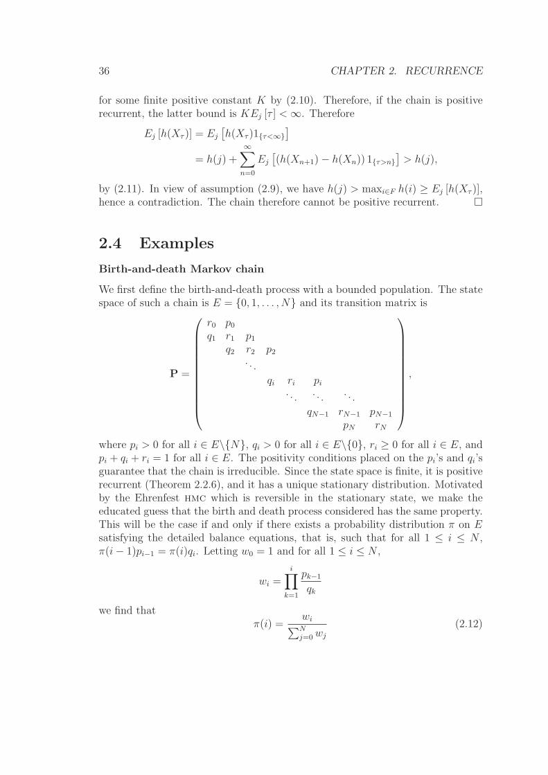
Birth-and-death Markov chain
We first define the birth-and-death process with a bounded population. The statespace of such a chain is E = {0, 1, . . . , N} and its transition matrix is
P =
r0 p0q1 r1 p1
q2 r2 p2. . .
qi ri pi. . . . . . . . .
qN−1 rN−1 pN−1
pN rN
,
where pi > 0 for all i ∈ E\{N}, qi > 0 for all i ∈ E\{0}, ri ≥ 0 for all i ∈ E, andpi + qi + ri = 1 for all i ∈ E. The positivity conditions placed on the pi’s and qi’sguarantee that the chain is irreducible. Since the state space is finite, it is positiverecurrent (Theorem 2.2.6), and it has a unique stationary distribution. Motivatedby the Ehrenfest hmc which is reversible in the stationary state, we make theeducated guess that the birth and death process considered has the same property.This will be the case if and only if there exists a probability distribution π on Esatisfying the detailed balance equations, that is, such that for all 1 ≤ i ≤ N ,π(i− 1)pi−1 = π(i)qi. Letting w0 = 1 and for all 1 ≤ i ≤ N ,
wi =i∏
k=1
pk−1
qk
we find thatπ(i) =
wi∑Nj=0wj
(2.12)
2.4. EXAMPLES 37
indeed satisfies the detailed balance equations and is therefore the (unique) sta-tionary distribution of the chain.
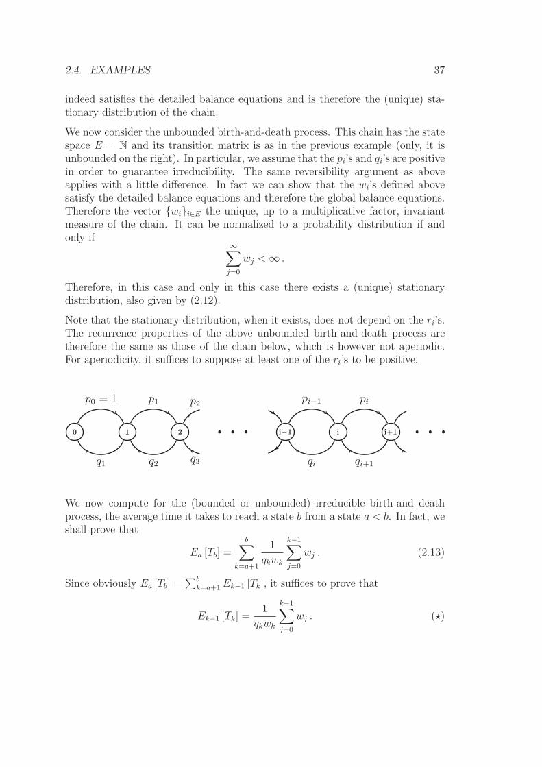
We now consider the unbounded birth-and-death process. This chain has the statespace E = N and its transition matrix is as in the previous example (only, it isunbounded on the right). In particular, we assume that the pi’s and qi’s are positivein order to guarantee irreducibility. The same reversibility argument as aboveapplies with a little difference. In fact we can show that the wi’s defined abovesatisfy the detailed balance equations and therefore the global balance equations.Therefore the vector {wi}i∈E the unique, up to a multiplicative factor, invariantmeasure of the chain. It can be normalized to a probability distribution if andonly if
∞∑
j=0
wj <∞ .
Therefore, in this case and only in this case there exists a (unique) stationarydistribution, also given by (2.12).
Note that the stationary distribution, when it exists, does not depend on the ri’s.The recurrence properties of the above unbounded birth-and-death process aretherefore the same as those of the chain below, which is however not aperiodic.For aperiodicity, it suffices to suppose at least one of the ri’s to be positive.
0 1 2 i−1 i i+1
p0 = 1 p1
q3
pi−1 pi
q1 q2 qi qi+1
p2
We now compute for the (bounded or unbounded) irreducible birth-and deathprocess, the average time it takes to reach a state b from a state a < b. In fact, weshall prove that
Ea [Tb] =b∑
k=a+1
1
qkwk
k−1∑
j=0
wj . (2.13)
Since obviously Ea [Tb] =∑b
k=a+1Ek−1 [Tk], it suffices to prove that
Ek−1 [Tk] =1
qkwk
k−1∑
j=0
wj . (⋆)
38 CHAPTER 2. RECURRENCE
For this, consider for any given k ∈ {0, 1, . . . , N} the truncated chain, which moveson the state space {0, 1, . . . , k} as the original chain, except in state k where itmoves one step down with probability qk and stays still with probability pk + rk.Write E for expectations of the modified chain. The unique stationary distributionof this chain is given by
πℓ =wℓ∑kj=0wℓ
for all 0 ≤ ℓ ≤ k. First-step analysis shows that Ek [Tk] = (rk + pk) × 1 +
qk
(1 + Ek−1 [Tk]
), that is
Ek [Tk] = 1 + qkEk−1 [Tk] .
Also
Ek [Tk] =1
πk=
1
wk
k∑
j=0
wj ,
and therefore, since Ek−1 [Tk] = Ek−1 [Tk], we have (⋆).
In the special case where (pj, qj, rj) = (p, q, r) for all j 6= 0, N , (p0, q0, r0) =
(p, q+ r, 0) and (pN , qN , rN) = (0, p+ r, q), we have wi =(
pq
)i
, and for 1 ≤ k ≤ N ,
Ek−1 [Tk] =1
q(
pq
)k
k−1∑
j=0
(p
q
)j
=1
p− q
(1−
(q
p
)k).
In the further particularization where p = q, wi = 1 for all i and
Ek−1 [Tk] =k
p.
The repair shop
During day n, Zn+1 machines break down, and they enter the repair shop onday n + 1. Every day one machine among those waiting for service is repaired.Therefore, denoting by Xn the number of machines in the shop on day n,
Xn+1 = (Xn − 1)+ + Zn+1, (2.14)
where a+ = max(a, 0). The sequence {Zn}n≥1 is assumed to be an iid sequence,independent of the initial state X0, with common probability distribution
P (Z1 = k) = ak, k ≥ 0
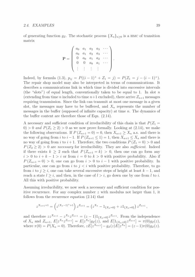
2.4. EXAMPLES 39
of generating function gZ . The stochastic process {Xn}n≥0 is a hmc of transitionmatrix
P =
a0 a1 a2 a3 · · ·a0 a1 a2 a3 · · ·0 a0 a1 a2 · · ·0 0 a0 a1 · · ·...
......
...
.
Indeed, by formula (1.3), pij = P ((i − 1)+ + Z1 = j) = P (Z1 = j − (i − 1)+).The repair shop model may also be interpreted in terms of communications. Itdescribes a communications link in which time is divided into successive intervals(the “slots”) of equal length, conventionally taken to be equal to 1. In slot n(extending from time n included to time n+1 excluded), there arrive Zn+1 messagesrequiring transmission. Since the link can transmit at most one message in a givenslot, the messages may have to be buffered, and Xn represents the number ofmessages in the buffer (supposed of infinite capacity) at time n. The dynamics ofthe buffer content are therefore those of Eqn. (2.14).
A necessary and sufficient condition of irreducibility of this chain is that P (Z1 =0) > 0 and P (Z1 ≥ 2) > 0 as we now prove formally. Looking at (2.14), we makethe following observations. If P (Zn+1 = 0) = 0, then Xn+1 ≥ Xn a.s. and there isno way of going from i to i− 1. If P (Zn+1 ≤ 1) = 1, then Xn+1 ≤ Xn and there isno way of going from i to i+1. Therefore, the two conditions P (Z1 = 0) > 0 andP (Z2 ≥ 2) > 0 are necessary for irreducibility. They are also sufficient. Indeedif there exists k ≥ 2 such that P (Zn+1 = k) > 0, then one can go form anyi > 0 to i + k − 1 > i or from i = 0 to k > 0 with positive probability. Also ifP (Zn+1 = 0) > 0, one can go from i > 0 to i − 1 with positive probability. Inparticular, one can go from i to j < i with positive probability. Therefore, to gofrom i to j ≥ i, one can take several successive steps of height at least k − 1, andreach a state l ≥ i, and then, in the case of l > i, go down one by one from l to i.All this with positive probability.
Assuming irreducibility, we now seek a necessary and sufficient condition for pos-itive recurrence. For any complex number z with modulus not larger than 1, itfollows from the recurrence equation (2.14) that
zXn+1+1 =(z(Xn−1)++1
)zZn+1 =
(zXn − 1{Xn=0} + z1{Xn=0}
)zZn+1 ,
and therefore zzXn+1 − zXnzZn+1 = (z − 1)1{Xn=0}zZn+1 . From the independence
of Xn and Zn+1, E[zXnzZn+1 ] = E[zXn ]gZ(z), and E[1{Xn=0}z
Zn+1 ] = π(0)gZ(z),where π(0) = P (Xn = 0). Therefore, zE[zXn+1 ]−gZ(z)E[zXn ] = (z−1)π(0)gZ(z).
40 CHAPTER 2. RECURRENCE
But in steady state, E[zXn+1 ] = E[zXn ] = gX(z), and therefore
gX(z) (z − gZ(z)) = π(0)(z − 1)gZ(z). (2.15)
This gives the generating function gX(z) =∑∞
i=0 π(i)zi, as long as π(0) is avail-
able. To obtain π(0), differentiate (2.15): g′X(z) (z − gZ(z)) + gX(z) (1− g′Z(z))= π(0) (gZ(z) + (z − 1)g′Z(z)), and let z = 1, to obtain, taking into account theequalities gX(1) = gZ(1) = 1 and g′Z(1) = E[Z],
π(0) = 1− E[Z]. (2.16)
But the stationary distribution of an irreducible hmc is positive, hence the neces-sary condition of positive recurrence:
E[Z1] < 1.
We now show this condition is also sufficient for positive recurrence. This followsimmediately from Pakes’s lemma, since for i ≥ 1, E[Xn+1−Xn |Xn = i] = E[Z]−1 < 0.
From (2.15) and (2.16), we have the generating function of the stationary distri-bution:
∞∑
i=0
π(i)zi = (1− E[Z])(z − 1)gZ(z)
z − gZ(z). (2.17)
If E[Z1] > 1, the chain is transient, as a simple argument based on the strong lawof large numbers shows. In fact, Xn = X0 +
∑nk=1 Zk − n +
∑nk=1 1{Xk=0}, and
therefore
Xn ≥n∑
k=1
Zk − n,
which tends to ∞ because, by the strong law of large numbers,
∑nk=1 Zk − n
n→ E[Z]− 1 > 0.
This is of course incompatible with recurrence.
We finally examine the case E[Z1] = 1, for which there are only two possibilitiesleft: transient or null recurrent. It turns out that the chain is null recurrent inthis case.
2.4. EXAMPLES 41
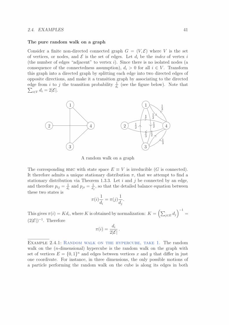
The pure random walk on a graph
Consider a finite non-directed connected graph G = (V, E) where V is the setof vertices, or nodes, and E is the set of edges. Let di be the index of vertex i(the number of edges “adjacent” to vertex i). Since there is no isolated nodes (aconsequence of the connectedness assumption), di > 0 for all i ∈ V . Transformthis graph into a directed graph by splitting each edge into two directed edges ofopposite directions, and make it a transition graph by associating to the directededge from i to j the transition probability 1
di(see the figure below). Note that∑
i∈V di = 2|E|.
1
2
3
4
1
2
3
4
1
13
13
12
12
12
12
13
A random walk on a graph
The corresponding hmc with state space E ≡ V is irreducible (G is connected).It therefore admits a unique stationary distribution π, that we attempt to find astationary distribution via Theorem 1.3.3. Let i and j be connected by an edge,and therefore pij =
1di
and pji =1dj, so that the detailed balance equation between
these two states is
π(i)1
di= π(j)
1
dj.
This gives π(i) = Kdi, whereK is obtained by normalization: K =(∑
j∈E dj
)−1
=
(2|E|)−1. Therefore
π(i) =di2|E| .
Example 2.4.1: Random walk on the hypercube, take 1. The randomwalk on the (n-dimensional) hypercube is the random walk on the graph withset of vertices E = {0, 1}n and edges between vertices x and y that differ in justone coordivate. For instance, in three dimensions, the only possible motions ofa particle performing the random walk on the cube is along its edges in both
42 CHAPTER 2. RECURRENCE
directions. Clearly, whatever be the dimension n ≥ 2, di =1nand the stationary
distribution is the uniform distribution.
The lazy random walk on the graph is, by definition, the Markov chain on V withthe transition probabilities pii =
12and for i, j ∈ V such that i and j are connected
by an edge of the graph, pi,i =12di
. This modified chain admits the same stationarydistribution as the original random walk. The difference is that the lazy version isalways aperiodic, whereas the original version maybe periodic.
2.5 Exercises
Exercise 2.5.1. Truncated hmc.Let P be a transition matrix on the countable state space E, with the positivestationary distribution π. Let A be a subset of the state space, and define thetruncation of P on A to be the transition matrix Q indexed by A and given by
qij = pij if i, j ∈ A, i 6= j,
qii = pii +∑
k∈A
pik.
Show that if (P, π) is reversible, then so is (Q, ππ(A)
).
Exercise 2.5.2. Extension to negative times.Let {Xn}n≥0 be a hmc with state space E, transition matrix P, and suppose thatthere exists a stationary distribution π > 0. Suppose moreover that the initialdistribution is π. Define the matrix Q = {qij}i,j∈E by (1.5). Construct {X−n}n≥1,independent of {Xn}n≥1 given X0, as follows:
P (X−1 = i1, X−2 = i2, . . . , X−k = ik |X0 = i,X1 = j1, . . . , Xn = jn)
= P (X−1 = i1, X−2 = i2, . . . , X−k = ik |X0 = i) = qii1qi1i2 · · · qik−1ik
for all k ≥ 1, n ≥ 1, i, i1, . . . , ik, j1, . . . , jn ∈ E. Prove that {Xn}n∈Z is a hmc withtransition matrix P and P (Xn = i) = π(i), for all i ∈ E, all n ∈ Z.
Exercise 2.5.3. Moving stones.Stones S1, . . . , SM are placed in line. At each time n a stone is selected at random,and this stone and the one ahead of it in the line exchange positions. If theselected stone is at the head of the line, nothing is changed. For instance, withM = 5: Let the current configuration be S2S3S1S5S4 (S2 is at the head of theline). If S5 is selected, the new situation is S2S3S5S1S4, whereas If S2 is selected,
2.5. EXERCISES 43
the configuration is not altered. At each step, stone Si is selected with probabilityαi > 0. Call Xn the situation at time n, for instance Xn = Si1 · · ·SiM , meaningthat stone Sij is in the jth position. Show that {Xn}n≥0 is an irreducible hmcand that it has a stationary distribution given by the formula
π(Si1 · · ·SiM ) = CαMi1αM−1i2
· · ·αiM ,
for some normalizing constant C.
Exercise 2.5.4. Aperiodicity.a. Show that an irreducible transition matrix P with at least one state i ∈ E suchthat pii > 0 is aperiodic.
b. Let P be an irreducible transition matrix on the finite state space E. Showthat a necessary and sufficient condition for P to be aperiodic is the existence ofan integer m such that Pm has all its entries positive.
c. Consider a hmc that is irreducible with period d ≥ 2. Show that the restrictionof the transition matrix to any cyclic class is irreducible. Show that the restrictionof Pd to any cyclic class is aperiodic.
Exercise 2.5.5. No stationary distribution.Show that the symmetric random walk on Z cannot have a stationary distribution.
Exercise 2.5.6. An interpretation of invariant measure.A countable number of particles move independently in the countable space E,each according to a Markov chain with the transition matrix P. Let An(i) be thenumber of particles in state i ∈ E at time n ≥ 0, and suppose that the randomvariables A0(i), i ∈ E, are independent Poisson random variables with respectivemeans µ(i), i ∈ E, where µ = {µ(i)}i∈E is an invariant measure of P. Show thatfor all n ≥ 1, the random variables An(i), i ∈ E, are independent Poisson randomvariables with respective means µ(i), i ∈ E.
Exercise 2.5.7. Doubly stochastic transition matrix.A stochastic matrix P on the state space E is called doubly stochastic if for allstates i,
∑j∈E pji = 1. Suppose in addition that P is irreducible, and that E
is infinite. Find the invariant measure of P. Show that P cannot be positiverecurrent.
Exercise 2.5.8. Return time to the initial state.Let τ be the first return time to inital state of an irreducible positive recurrenthmc {Xn}n≥0, that is,
τ = inf{n ≥ 1;Xn = X0},
44 CHAPTER 2. RECURRENCE
with τ = +∞ if Xn 6= X0 for all n ≥ 1. Compute the expectation of τ whenthe initial distribution is the stationary distribution π. Conclude that it is finiteif and only if E is finite. When E is infinite, is this in contradiction to positiverecurrence?
Chapter 3
Long-run behaviour
3.1 Ergodic theorem
An important application of the strong law of large numbers is to the ergodic theo-rem for Markov chains. This theorem gives conditions guaranteeing that empiricalaverages of the type
1
N
N∑
k=1
g(Xk, . . . , Xk+L)
converge to probabilistic averages. As a matter of fact, if the chain is irreduciblepositive recurrent with the stationary distribtion π, the above empirical aver-age converges Pµ-almost-surely to Eπ[g(X0, . . . , XL)] for any initial distribution µ(Corollary 3.1.2), at least if Eπ[|g(X0, . . . , XL)|] <∞.
We shall obtain this result as a corollary of the following proposition concerningirreducible recurrent (not necessarily positive recurrent) hmc’s.
Let {Xn}n≥0 be an irreducible recurrent hmc, and let x denote the canonicalinvariant measure associated with state 0 ∈ E,
xi = E0
[∑
n≥1
1{Xn=i}1{n≤T0}
], (3.1)
where T0 is the return time to 0. Define for n ≥ 1, ν(n) :=∑n
k=1 1{Xk=0}.
45
46 CHAPTER 3. LONG-RUN BEHAVIOUR
Theorem 3.1.1 Let f : E → R be such that
∑
i∈E
|f(i)|xi <∞. (3.2)
Then, for any initial distribution µ, Pµ-a.s.,
limN↑∞
1
ν(N)
N∑
k=1
f(Xk) =∑
i∈E
f(i)xi. (3.3)
Proof. Let T0 = τ1, τ2, τ3, . . . be the successive return times to state 0, and define
Up =
τp+1∑
n=τp+1
f(Xn).
By the independence property of the regenerative cycles, {Up}p≥1 is an iid se-quence. Moreover, assuming f ≥ 0 and using the strong Markov property,
E[U1] = E0
[T0∑
n=1
f(Xn)
]
= E0
[T0∑
n=1
∑
i∈E
f(i)1{Xn=i}
]=
∑
i∈E
f(i)E0
[T0∑
n=1
1{Xn=i}
]
=∑
i∈E
f(i)xi.
By hypothesis, this quantity is finite, and threfore the strong law of large numbersapplies, to give
limn↑∞
1
n
n∑
p=1
Up =∑
i∈E
f(i)xi,
that is,
limn↑∞
1
n
τn+1∑
k=T0+1
f(Xk) =∑
i∈E
f(i)xi. (3.4)
Observing that
τν(n) ≤ n < τν(n)+1,
we have ∑τν(n)
k=1 f(Xk)
ν(n)≤
∑nk=1 f(Xk)
ν(n)≤
∑τν(n)+1
k=1 f(Xi)
ν(n).
3.1. ERGODIC THEOREM 47
Since the chain is recurrent, limn↑∞ ν(n) = ∞, and therefore, from (3.4), theextreme terms of the above chain of inequality tend to
∑i∈E f(i)xi as n goes to
∞, and this implies (3.3). The case of a function f of arbitrary sign is obtained byconsidering (3.3) written separately for f+ = max(0, f) and f− = max(0,−f), andthen taking the difference of the two equalities obtained this way. The differenceis not an undetermined form ∞−∞ due to hypothesis (3.2). �
Corollary 3.1.1 Let {Xn}n≥0 be an irreducible positive recurrent Markov chainwith the stationary distribution π, and let f : E → R be such that
∑
i∈E
|f(i)|π(i) <∞. (3.5)
Then for any initial distribution µ, Pµ-a.s.,
limn↑∞
1
N
N∑
k=1
f(Xk) =∑
i∈E
f(i)π(i). (3.6)
Proof. Apply Theorem 3.1.1 to f ≡ 1. Condition (3.2) is satisfied, since in thepositive recurrent case,
∑i∈E xi = E0[T0] <∞. Therefore, Pµ-a.s.,
limN↑∞
N
ν(N)=
∑
j∈E
xj.
Now, f satisfying (3.5) also satisfies (3.2), since x and π are proportional, andtherefore, Pµ-a.s.,
limN↑∞
1
ν(N)
N∑
k=1
f(Xk) =∑
i∈E
f(i)xi.
Combination of the above equalities gives, Pµ-a.s.,
limN→∞
1
N
N∑
k=1
f(Xk) = limN→∞
ν(N)
N
1
ν(N)
N∑
k=1
f(Xk) =
∑i∈E f(i)xi∑
j∈E xj,
from which (3.6) follows, since π is obtained by normalization of x. �
Corollary 3.1.2 Let {Xn}n≥1 be an irreducible positive recurrent Markov chainwith the stationary distribution π, and let g : EL+1 → R be such that
∑
i0,...,iL
|g(i0, . . . , iL)|π(i0)pi0i1 · · · piL−1iL <∞
48 CHAPTER 3. LONG-RUN BEHAVIOUR
(see Example 3.5.8) Then for all initial distributions µ, Pµ-a.s.
lim1
N
N∑
k=1
g(Xk, Xk+1, . . . , Xk+L) =∑
i0,i1,...,iL
g(i0, i1, . . . , iL)π(i0)pi0i1 · · · piL−1iL .
Proof. Apply Corollary 3.1.1 to the snake chain {(Xn, Xn+1, . . . , Xn+L)}n≥0,which is irreducible recurrent and admits the stationary distribution
π(i0)pi0i1 · · · piL−1iL .
�
Note that
∑
i0,i1,...,iL
g(i0, i1, . . . , iL)π(i0)pi0i1 · · · piL−1iL = Eπ[g(X0, . . . , XL)]
3.2 Convergence in variation
The purpose is to bound the “distance” between two probability distributions,this distance being the variation distance. One interest of this, among others, isto replace a random element by another for which computations may be easier.
Definition 3.2.1 Let E be a countable space. The distance in variation betweentwo probability distributions α and β on E is the quantity
dV (α, β) :=1
2
∑
i∈E
|α(i)− β(i)|. (3.7)
That dV is indeed a distance is clear.
Lemma 3.2.1 Let α and β be two probability distributions on the same countablespace E. Then
dV (α, β) = supA⊆E
{α(A)− β(A)}
= supA⊆E
{|α(A)− β(A)|} .
3.2. CONVERGENCE IN VARIATION 49
Proof. For the second equality observe that for each subset A there is a subset Bsuch that |α(A)− β(A)| = α(B)− β(B) (take B = A or A). For the first equality,write
α(A)− β(A) =∑
i∈E
1A(i){α(i)− β(i)}
and observe that the right-hand side is maximal for A = {i ∈ E; α(i) > β(i)}.Therefore, with g(i) = α(i)− β(i),
supA⊆E
{α(A)− β(A)} =∑
i∈E
g+(i) =1
2
∑
i∈E
|g(i)| ,
where the equality∑
i∈E g(i) = 0 was taken into account. �
The distance in variation between two random variables X and Y with values inE is the distance in variation between their probability distributions, and it isdenoted (with a slight abuse of notation) by dV (X, Y ). Therefore
dV (X, Y ) :=1
2
∑
i∈E
|P (X = i)− P (Y = i)| .
The distance in variation between a random variable X with values in E and aprobability distribution α on E denoted (again with a slight abuse of notation) bydV (X,α) is defined by
dV (X,α) :=1
2
∑
i∈E
|P (X = i)− α(i)| .
The coupling inequality
Coupling two discrete probability distributions π′ on E ′ and π′′ on E ′′ consists inthe construction of a probability distribution π on E := E ′ × E ′′ such that themarginal distributions of π on E ′ and E ′′ respectively are π′ and π′′, that is
∑
j∈E′′
π(i, j) = π′(i) and∑
i∈E′
π(i, j) = π′′(j) .
For two probability distributions α and β on the countable set E, let D(α, β) bethe collection of pairs of random variables (X, Y ) taking their values in E × E,and with marginal distributions α and β, that is,
P (X = i) = α(i), P (Y = i) = β(i) . (3.8)
50 CHAPTER 3. LONG-RUN BEHAVIOUR
Theorem 3.2.1 For any pair (X, Y ) ∈ D(α, β), we have the fundamental cou-pling inequality
dV (α, β) ≤ P (X 6= Y ), (3.9)
and equality is attained by some pair (X, Y ) ∈ D(α, β), which is then said torealize maximal coincidence.
Proof. For arbitrary A ⊂ E,
P (X 6= Y ) ≥ P (X ∈ A, Y ∈ A) = P (X ∈ A)−P (X ∈ A, Y ∈ A) ≥ P (X ∈ A)−P (Y ∈ A),
and therefore
P (X 6= Y ) ≥ supA⊂E
{P (X ∈ A)− P (Y ∈ A)} = dV (α, β).
We now construct (X, Y ) ∈ D(α, β) realizing equality. Let U,Z, V , and W beindependent random variables; U takes its values in {0, 1}, and Z, V,W take theirvalues in E. The distributions of these random variables are given by
P (U = 1) = 1− dV (α, β),
P (Z = i) = (α(i) ∧ β(i))/ (1− dV (α, β)) ,
P (V = i) = (α(i)− β(i))+/dV (α, β) ,
P (W = i) = (β(i)− α(i))+/dV (α, β) .
Observe that P (V = W ) = 0. Defining
(X, Y ) = (Z,Z) if U = 1
= (V,W ) if U = 0 ,
we have
P (X = i) = P (U = 1, Z = i) + P (U = 0, V = i)
= P (U = 1)P (Z = i) + P (U = 0)P (V = i)
= α(i) ∧ β(i) + (α(i)− β(i))+ = α(i),
and similarly, P (Y = i) = β(i). Therefore, (X, Y ) ∈ D(α, β). Also, P (X = Y ) =P (U = 1) = 1− dV (α, β), that is P (X 6= Y ) = dV (α, β). �
A sequence {Xn}n≥1 of discrete random variables with values in E is said toconverge in distribution to the probability distribution π on E if for all i ∈ E,limn↑∞ P (Xn = i) = π(i). It is said to converge in variation to this distribution if
limn↑∞
∑
i∈E
|P (Xn = i)− π(i)| = 0 .
3.2. CONVERGENCE IN VARIATION 51
Observe that Definition 3.2.3 concerns only the marginal distributions of thestochastic process, not the stochastic process itself. Therefore, if there exists an-
other stochastic process {X ′n}n≥0 such that Xn
D∼ X ′n for all n ≥ 0, and if there
exists a third one {X ′′n}n≥0 such that X ′′
nD∼ π for all n ≥ 0, then (3.13) follows
fromlimn↑∞
dV (X′n, X
′′n) = 0. (3.10)
This trivial observation is useful because of the resulting freedom in the choice of{X ′
n} and {X ′′n}. An interesting situation occurs when there exists a finite random
time τ such that X ′n = X ′′
n for all n ≥ τ .
Definition 3.2.2 Two stochastic processes {X ′n}n≥0 and {X ′′
n}n≥0 taking their val-ues in the same state space E are said to couple if there exists an almost surelyfinite random time τ such that
n ≥ τ ⇒ X ′n = X ′′
n. (3.11)
The random variable τ is called a coupling time of the two processes.
Theorem 3.2.2 For any coupling time τ of {X ′n}n≥0 and {X ′′
n}n≥0, we have thecoupling inequality
dV (X′n, X
′′n) ≤ P (τ > n) . (3.12)
Proof. For all A ⊆ E,
P (X ′n ∈ A)− P (X ′′
n ∈ A) = P (X ′n ∈ A, τ ≤ n) + P (X ′
n ∈ A, τ > n)
− P (X ′′n ∈ A, τ ≤ n)− P (X ′′
n ∈ A, τ > n)
= P (X ′n ∈ A, τ > n)− P (X ′′
n ∈ A, τ > n)
≤ P (X ′n ∈ A, τ > n) ≤ P (τ > n).
Inequality (3.12) then follows from Lemma 3.2.1. �
Therefore, if the coupling time is P-a.s. finite, that is limn↑∞ P (τ > n) = 0,
limn↑∞
dV (Xn, π) = limn↑∞
dV (X′n, X
′′n) = 0 .
Definition 3.2.3 (A) A sequence {αn}n≥0 of probability distributions on E is saidto converge in variation to the probability distribution β on E if
limn↑∞
dV (αn, β) = 0 .
52 CHAPTER 3. LONG-RUN BEHAVIOUR
(B) An E-valued random sequence {Xn}n≥0 such that for some probability dis-tribution π on E,
limn↑∞
dV (Xn, π) = 0, (3.13)
is said to converge in variation to π.
Kolmogorov’s hmc convergence theorem
Consider a hmc that is irreducible and positive recurrent. If its initial distributionis the stationary distribution, it keeps the same distribution at all times. The chainis then said to be in the stationary regime, or in equilibrium, or in steady state.A question arises naturally: What is the long-run behavior of the chain when theinitial distribution µ is arbitrary? For instance, will it converge to equilibrium? inwhat sense? The classical form of the result is that for arbitrary states i and j,
limn↑∞
pij(n) = π(j) , (3.14)
if the chain is ergodic, according to the following definition:
Definition 3.2.4 An irreducible positive recurrent and aperiodic hmc is calledergodic.
If the state space is finite, computation of the n-th iterate of the transition matrixP is all that we need, in principle, to prove (3.14). Such computation requires someknowledge of the eigenstructure of P, and there is a famous result of linear algebra,the Perron–Frobenius theorem, that does the work. We shall give the details inSubsection 3.2. However, in the case of infinite state space, linear algebra fails toprovide the answer, and recourse to other methods is necessary.
In fact, (3.14) can be drastically improved:
Theorem 3.2.3 Let {Xn}n≥0 be an ergodic hmc on the countable state space Ewith transition matrix P and stationary distribution π, and let µ be an arbitraryinitial distribution. Then
limn↑∞
∑
i∈E
|Pµ(Xn = i)− π(i)| = 0,
and in particular, for all j ∈ E,
limn↑∞
∑
i∈E
|pji(n)− π(i)| = 0.
The proof will be given in Section 3.2.
3.2. CONVERGENCE IN VARIATION 53
The coupling proof
The proof of Theorem 3.2.3 will be given via the coupling method.
Proof. We prove that, for all probability distributions µ and ν on E,
limn↑∞
dV (µTPn, νTPn) = 0.
The announced results correspond to the particular case where ν is the stationarydistribution π, and particularizing further, µ = δj. From the discussion precedingDefinition 3.2.2, it suffices to construct two coupling chains with initial distribu-tions µ and ν, respectively. This is done in the next lemma. �
Lemma 3.2.2 Let {X(1)n }n≥0 and {X(2)
n }n≥0 be two independent ergodic hmcswith the same transition matrix P and initial distributions µ and ν, respectively.Let τ = inf{n ≥ 0; X
(1)n = X
(2)n }, with τ = ∞ if the chains never intersect. Then
τ is, in fact, almost surely finite. Moreover, the process {X ′n}n≥0 defined by
X ′n =
{X
(1)n if n ≤ τ,
X(2)n if n ≥ τ
(3.15)
is an hmc with transition matrix P (see the figure below). FIGURE?
Proof. Step 1. Consider the product hmc {Zn}n≥0 defined by Zn = (X(1)n , X
(2)n ).
It takes values in E ×E, and the probability of transition from (i, k) to (j, ℓ) in nsteps is pij(n)pkℓ(n). We first show that this chain is irreducible. The probabilityof transition from (i, k) to (j, ℓ) in n steps is pij(n)pkℓ(n). Since P is irreducible andaperiodic, by Theorem 1.2.2, there exists m such that for all pairs (i, j) and (k, ℓ),n ≥ m implies pij(n)pkℓ(n) > 0. This implies irreducibility. (Note the essentialrole of aperiodicity. A simple counterexample is that of the the symmetric randomwalk on , which is irreducible but of period 2. The product of two indepencentsuch hmc’s is the symmetric random walk on 2 which has two communicationsclasses.)
Step 2. Next we show that the two independent chains meet in finite time. Clearly,the distribution σ defined by σ(i, j) := π(i)π(j) is a stationary distribution forthe product chain, where π is the stationary distribution of P. Therefore, bythe stationary distribution criterion, the product chain is positive recurrent. Inparticular, it reaches the diagonal of E2 in finite time, and consequently, P (τ <∞) = 1.
54 CHAPTER 3. LONG-RUN BEHAVIOUR
It remains to show that {X ′n}n≥0 given by (3.15) is an hmc with transition matrix
P. For this we use the following lemma.
Lemma 3.2.3 Let X10 , X
20 , Z
1n, Z
2n (n ≥ 1), be independent random variables, and
suppose moreover that Z1n, Z
2n (n ≥ 1) are identically distributed. Let τ be a non-
negative integer-valued random variable such that for allm ∈ , the event {τ = m}is expressible in terms of X1
0 , X20 , Z
1n, Z
2n (n ≤ m). Define the sequence {Zn}n≥1 by
Zn = Z1n if n ≤ τ
= Z2n if n > τ
Then, {Zn}n≥1 has the same distribution as {Z1n}n≥1 and is independent of X1
0 , X20 .
Proof. For any sets sets C1, C2, A1, . . . , Ak in the appropriate spaces,
P (X10 ∈ C1, X
20 ∈ C2, Zℓ ∈ Aℓ, 1 ≤ ℓ ≤ k)
=k∑
m=0
P (X10 ∈ C1, X
20 ∈ C2, Zℓ ∈ Aℓ, 1 ≤ ℓ ≤ k, τ = m)
+ P (X10 ∈ C1, X
20 ∈ C2, Z1 ∈ A1, . . . , Zk ∈ Ak, τ > k)
=k∑
m=0
P (X10 ∈ C1, X
20 ∈ C2, Z
1ℓ ∈ Aℓ, 1 ≤ ℓ ≤ m, τ = m,Z2
r ∈ Ar,m+ 1 ≤ r ≤ k)
+ P (X10 ∈ C1, X
20 ∈ C2, Z
1ℓ ∈ Aℓ, 1 ≤ ℓ ≤ k, τ > k) .
Since the event {τ = m} is independent of Z2m+1 ∈ Am+1, . . . , Z
2k ∈ Ak (k ≥ m),
=k∑
m=0
P (X10 ∈ C1, X
20 ∈ C2, Z
1ℓ ∈ Aℓ, 1 ≤ ℓ ≤ m, τ = m)P (Z2
r ∈ Ar,m+ 1 ≤ r ≤ k)
+ P (X10 ∈ C1, X
20 ∈ C2, Z
1ℓ ∈ Aℓ, 1 ≤ ℓ ≤ k, τ > k)
=k∑
m=0
P (X10 ∈ C1, X
20 ∈ C2, Z
1ℓ ∈ Aℓ, 1 ≤ ℓ ≤ m, τ = m,Z1
r ∈ Ar,m+ 1 ≤ r ≤ k)
+ P (X10 ∈ C1, X
20 ∈ C2, Z
1ℓ ∈ Aℓ, 1 ≤ ℓ ≤ k, τ > k)
= P (X10 ∈ C1, X
20 ∈ C2, Z
11 ∈ A1, . . . , Z
1k ∈ Ak) .
�
Step 3. We now complete the proof. The statement of the theorem concernsonly the distributions of {X1
n}n≥0 and {X2n}n≥0, and therefore we can assume a
representationXℓ
n+1 = f(Xℓn, Z
ℓn+1) (ℓ = 1, 2) ,
3.2. CONVERGENCE IN VARIATION 55
where X10 , X
20 , Z
1n, Z
2n (n ≥ 1) satisfy the conditions stated in Lemma 3.2.3. The
random time τ satisfies the condition of Lemma 3.2.3. Defining {Zn}n≥1 in thesame manner as in this lemma, we therefore have
Xn+1 = f(Xn, Zn+1) ,
which proves the announced result. �
Null recurrent case
Theorem 3.2.3 concerns the positive recurrent case. In the null recurrent case wehave Orey’s theorem:
Theorem 3.2.4 Let P be an irreducible null recurrent transition matrix on E.Then for all i, j ∈ E,
limn↑∞
pij(n) = 0. (3.16)
Perron–Frobenius
When the state space of a hmc is finite, we can rely on the standard results of linearalgebra to study the asymptotic behavior of the n-step transition matrix Pn, whichdepends on the eigenstructure of P. The Perron–Frobenius theorem detailing theeigenstructure of non-negative matrices is therefore all that is needed, at least intheory.
The main result of Perron and Frobenius is that convergence to steady state ofan ergodic finite state space hmc is geometric, with relative speed equal to thesecond-largest eigenvalue modulus (slem). Even if there are a few interestingmodels, especially in biology, where the eigenstructure of the transition matrixcan be extracted, this situation remains nevertheless exceptional. It is thereforeimportant to find estimates of the slem.
From the basic results of the theory of matrices relative to eigenvalues and eigen-vectors we quote the following one, relative to a square matrix A of dimension rwith distinct eigenvalues denoted λ1, . . . , λr. Let u1, . . . , ur and v1, . . . , vr be theassociated sequences of left and right eigenvectors, respectively. Then, u1, . . . , urform an independent collection of vectors, and so do v1, . . . , vr. Also, uTi vj = 0 ifi 6= j. Since eigenvectors are determined up to multiplication by an arbitrary non-null scalar, one can choose them in such a way that uTi vi = 1 for all i, 1 ≤ i ≤ r.We then have the spectral decomposition
An =r∑
i=1
λni viuTi . (3.17)
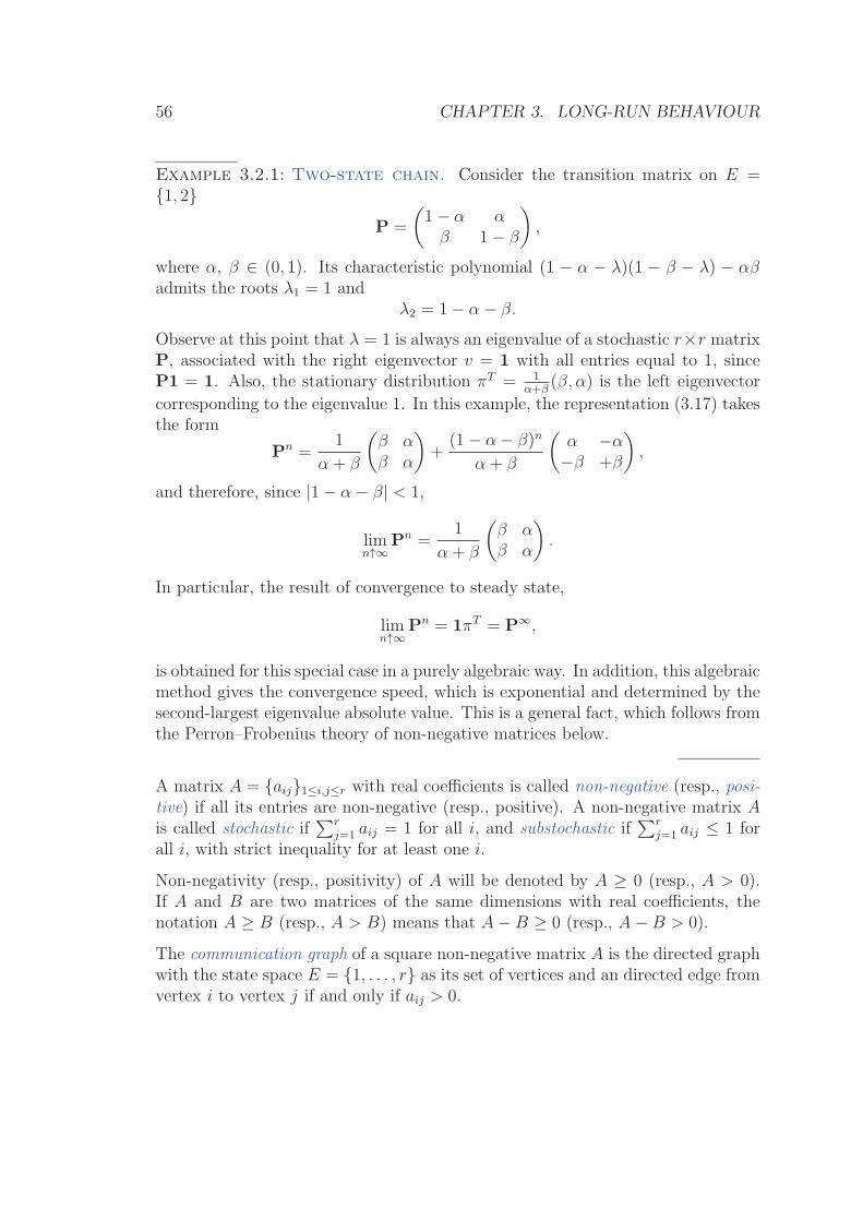
56 CHAPTER 3. LONG-RUN BEHAVIOUR
Example 3.2.1: Two-state chain. Consider the transition matrix on E ={1, 2}
P =
(1− α αβ 1− β
),
where α, β ∈ (0, 1). Its characteristic polynomial (1 − α − λ)(1 − β − λ) − αβadmits the roots λ1 = 1 and
λ2 = 1− α− β.
Observe at this point that λ = 1 is always an eigenvalue of a stochastic r×r matrixP, associated with the right eigenvector v = 1 with all entries equal to 1, sinceP1 = 1. Also, the stationary distribution πT = 1
α+β(β, α) is the left eigenvector
corresponding to the eigenvalue 1. In this example, the representation (3.17) takesthe form
Pn =1
α + β
(β αβ α
)+
(1− α− β)n
α + β
(α −α−β +β
),
and therefore, since |1− α− β| < 1,
limn↑∞
Pn =1
α + β
(β αβ α
).
In particular, the result of convergence to steady state,
limn↑∞
Pn = 1πT = P∞,
is obtained for this special case in a purely algebraic way. In addition, this algebraicmethod gives the convergence speed, which is exponential and determined by thesecond-largest eigenvalue absolute value. This is a general fact, which follows fromthe Perron–Frobenius theory of non-negative matrices below.
A matrix A = {aij}1≤i,j≤r with real coefficients is called non-negative (resp., posi-tive) if all its entries are non-negative (resp., positive). A non-negative matrix Ais called stochastic if
∑rj=1 aij = 1 for all i, and substochastic if
∑rj=1 aij ≤ 1 for
all i, with strict inequality for at least one i.
Non-negativity (resp., positivity) of A will be denoted by A ≥ 0 (resp., A > 0).If A and B are two matrices of the same dimensions with real coefficients, thenotation A ≥ B (resp., A > B) means that A−B ≥ 0 (resp., A−B > 0).
The communication graph of a square non-negative matrix A is the directed graphwith the state space E = {1, . . . , r} as its set of vertices and an directed edge fromvertex i to vertex j if and only if aij > 0.
3.2. CONVERGENCE IN VARIATION 57
A non-negative square matrix A is called irreducible (resp., irreducible aperiodic) ifit has the same communication graph as an irreducible (resp., irreducible aperiodic)stochastic matrix. It is called primitive if there exists an integer k such that Ak > 0.
Example 3.2.2: A non-negative matrix is primitive if and only if it is irreducibleand aperiodic (Exercise ??).
Let A be a non-negative primitive r × r matrix. There exists a real eigenvalueλ1 with algebraic as well as geometric multiplicity one such that λ1 > 0, andλ1 > |λj| for any other eigenvalue λj. Moreover, the left eigenvector u1 andthe right eigenvector v1 associated with λ1 can be chosen positive and such thatuT1 v1 = 1.
Let λ2, λ3, . . . , λr be the eigenvalues of A other than λ1 ordered in such a way that
λ1 > |λ2| ≥ · · · ≥ |λr| (3.18)
We may always order the eigenvalues in such a way that if |λ2| = |λj| for somej ≥ 3, then m2 ≥ mj, where mj is the algebraic multiplicity of λj. Then
An = λn1v1uT1 +O(nm2−1|λ2|n). (3.19)
If in addition, A is stochastic (resp., substochastic), then λ1 = 1 (resp., λ1 < 1).
If A is stochastic and irreducible with period d > 1, then there are exactly ddistinct eigenvalues of modulus 1, namely the d-th roots of unity, and all othereigenvalues have modulus strictly less than 1.
Example 3.2.3: Convergence rates via Perron–Frobenius. If P is atransition matrix on E = {1, . . . , r} that is irreducible and aperiodic, and thereforeprimitive, then
v1 = 1, u1 = π,
where π is the unique stationary distribution. Therefore
Pn = 1πT +O(nm2−1|λ2|n), (3.20)
which generalizes the observation in Example 3.2.1.
58 CHAPTER 3. LONG-RUN BEHAVIOUR
3.3 Monte Carlo
Recall the method of the inverse in order to generate a discrete random variableZ with distribution P (Z = ai) = pi (0 ≤ i ≤ K). A crude algorithm based onthis method would perform successively the tests U ≤ p0?, U ≤ p0+ p1?, . . ., untilthe answer is positive. Although very simple in principle, the inverse method hasthe following drawbacks when the size r of the state space E is large.
(a) Problems arise that are due to the small size of the intervals partitioning[0, 1] and to the cost of precision in computing.
(b) Another situation is that in which the probability density π is known onlyup to a normalizing factor, that is, π(i) = Kπ(i), and when the sum
∑i∈E π(i) =
K−1 that gives the normalizing factor is prohibitively difficult to compute. Inphysics, this is a frequent case.
Approximate sampling
The quest for a random generator without these ailments is at the origin of theMonte Carlo Markov chain (mcmc) sampling methodology. The basic principleis the following. One constructs an irreducible aperiodic hmc {Xn}n≥0 with statespace E and stationary distribution π. Since the state space is finite, the chainis ergodic, and therefore, by Theorem 3.2.3, for any initial distribution µ and alli ∈ E,
limn→∞
Pµ(Xn = i) = π(i) . (3.21)
Therefore, when n is “large,” we can consider that Xn has a distribution close toπ.
The first task is that of designing the mcmc algorithm. One must find an ergodictransition matrix P on E, the stationary distribution of which π. In the MonteCarlo context, the transition mechanism of the chain is called a sampling algorithm,and the asymptotic distribution π is called the target distribution, or sampleddistribution.
There are infinitely many transition matrices with a given target distribution, andamong them there are infinitely many that correspond to a reversible chain, thatis, such that
π(i)pij = π(j)pji.
We seek solutions of the formpij = qijαij (3.22)
for j 6= i, where Q = {qij}i,j∈E is an arbitrary irreducible transition matrix onE, called the candidate-generator matrix. When the present state is i, the next
3.3. MONTE CARLO 59
tentative state j is chosen with probability qij. When j 6= i, this new state isaccepted with probability αij. Otherwise, the next state is the same state i. Hence,the resulting probability of moving from i to j when i 6= j is given by (3.22). Itremains to select the acceptance probabilities αij .
Example 3.3.1: Metropolis, take 1. In the Metropolis algorithm
αij = min
(1,π(j)qjiπ(i)qij
).
In Physics, it often arises, and we shall understand why later, that the distributionπ is of the form 3.23.
π(i) =e−U(i)
Z, (3.23)
where U : E → is the “energy function” and Z is the “partition function”,the normalizing constant ensuring that π is indeed a probability vector. Theacceptance probability of the transition from i to j is then, assuming the candidate-generating matrix to be symmetric,
αij = min(1, e−(U(j)−U(i))
).
Example 3.3.2: Barker’s algorithm. The Barker algorithm, corresponds tothe choice
αij =π(j)qji
π(j)qji + π(i)qij. (3.24)
When the distribution π is of the form 3.23, the acceptance probability of the tran-sition from i to j is, assuming the candidate-generating matrix to be symmetric,
αij =e−U(i)
e−U(i) + e−U(j).
This corresponds to the basic principle of statistical thermodynamics: when twostates 1 and 2 with energies E1 and E2, choose 1 with probability e−E1
e−E1+e−E2.
Example 3.3.3: The Gibbs algorithm. Consider a multivariate probabilitydistribution
π(x(1), . . . , x(N))
60 CHAPTER 3. LONG-RUN BEHAVIOUR
on a set E = ΛN , where Λ is countable. The basic step of the Gibbs sampler forthe multivariate distribution π consists in selecting a coordinate number 1 ≤ i ≤,at random, and choosing the new value y(i) of the corresponding coordinate, giventhe present values x(1), . . . , x(i − 1), x(i + 1), . . . , x(N) of the other coordinates,with probability
π(y(i) | x(1), . . . , x(i− 1), x(i+ 1), . . . , x(N)).
One checks as above that π is the stationary distribution of the correspondingchain.
Exact sampling
We attempt to construct an exact sample of a given π on a finite state space E,that is a random variable Z such that P (Z = i) = π(i) for all i ∈ E. The followingalgorithm (Propp–Wilson algorithm) is based on a coupling idea. One starts asusual from an ergodic transition matrix P with stationary distribution π, just asin the classical mcmc method.
The algorithm is based on a representation of P in terms of a recurrence equation,that is, for given a function f and an iid sequence {Zn}n≥1 independent of theinitial state, the chain satisfies the recurrence
Xn+1 = f(Xn, Zn+1) . (3.25)
The Propp-Wilson algorithm constructs a family of hmc with this transition ma-trix with the help of a unique iid sequence of random vectors {Yn}n∈ , called theupdating sequence, where Yn = (Zn+1(1), · · · , Zn+1(r)) is a r-dimensional randomvector, and where the coordinates Zn+1(i) have a common distribution, that of Z1.For each N ∈ and each k ∈ E, a process {XN
n (k)}n≥N is defined recursively by:
XNN (k) = k,
and, for n ≥ N ,XN
n+1(k) = f(XNn (k), Zn+1(X
Nn (k)).
(Thus, if the chain is in state i at time n, it will be at time n + 1 in state j =f(i, Zn+1(i).) Each of these processes is therefore a hmc with the transition matrixP. Note that for all k, ℓ ∈ E, and all M,N ∈ , the hmc’s {XN
n (k)}n≥N and{XM
n (ℓ)}n≥M use at any time n ≥ max(M,N) the same updating random vectorYn+1.
If, in addition to the independence of {Yn}n∈ , the components Zn+1(1), Zn+1(2),. . ., Zn+1(r) are, for each n ∈ , independent, we say that the updating is compo-nentwise independent.
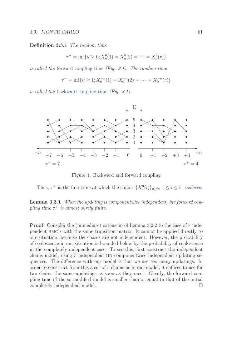
3.3. MONTE CARLO 61
Definition 3.3.1 The random time
τ+ = inf{n ≥ 0;X0n(1) = X0
n(2) = · · · = X0n(r)}
is called the forward coupling time (Fig. 3.1). The random time
τ− = inf{n ≥ 1;X−n0 (1) = X−n
0 (2) = · · · = X−n0 (r)}
is called the backward coupling time (Fig. 3.1).
00
12345
E
−1−2−3−4−5−6−7−n
+1 +2 +3 +4+n
τ− = 7 τ+ = 4
Figure 1. Backward and forward coupling
Thus, τ+ is the first time at which the chains {X0n(i)}n≥0, 1 ≤ i ≤ r, coalesce.
Lemma 3.3.1 When the updating is componentwise independent, the forward cou-pling time τ+ is almost surely finite.
Proof. Consider the (immediate) extension of Lemma 3.2.2 to the case of r inde-pendent hmc’s with the same transition matrix. It cannot be applied directly toour situation, because the chains are not independent. However, the probabilityof coalescence in our situation is bounded below by the probability of coalescencein the completely independent case. To see this, first construct the independentchains model, using r independent iid componentwise independent updating se-quences. The difference with our model is that we use too many updatings. Inorder to construct from this a set of r chains as in our model, it suffices to use fortwo chains the same updatings as soon as they meet. Clearly, the forward cou-pling time of the so modified model is smaller than or equal to that of the initialcompletely independent model. �
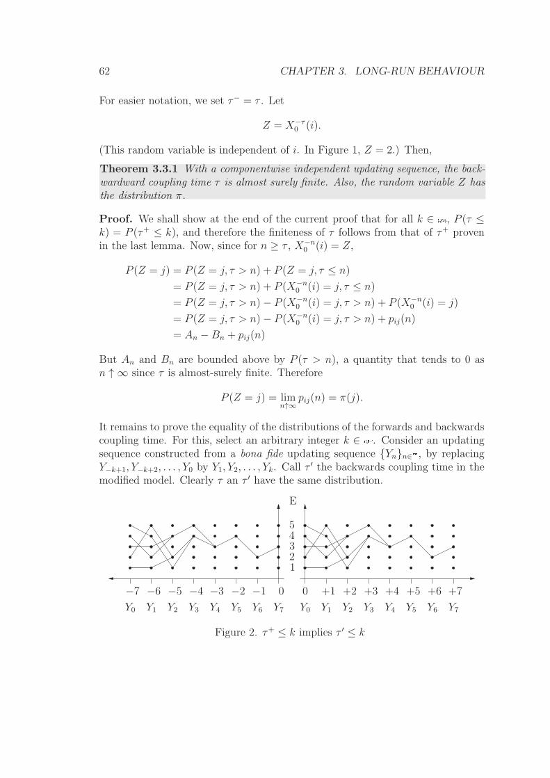
62 CHAPTER 3. LONG-RUN BEHAVIOUR
For easier notation, we set τ− = τ . Let
Z = X−τ0 (i).
(This random variable is independent of i. In Figure 1, Z = 2.) Then,
Theorem 3.3.1 With a componentwise independent updating sequence, the back-wardward coupling time τ is almost surely finite. Also, the random variable Z hasthe distribution π.
Proof. We shall show at the end of the current proof that for all k ∈ , P (τ ≤k) = P (τ+ ≤ k), and therefore the finiteness of τ follows from that of τ+ provenin the last lemma. Now, since for n ≥ τ , X−n
0 (i) = Z,
P (Z = j) = P (Z = j, τ > n) + P (Z = j, τ ≤ n)
= P (Z = j, τ > n) + P (X−n0 (i) = j, τ ≤ n)
= P (Z = j, τ > n)− P (X−n0 (i) = j, τ > n) + P (X−n
0 (i) = j)
= P (Z = j, τ > n)− P (X−n0 (i) = j, τ > n) + pij(n)
= An −Bn + pij(n)
But An and Bn are bounded above by P (τ > n), a quantity that tends to 0 asn ↑ ∞ since τ is almost-surely finite. Therefore
P (Z = j) = limn↑∞
pij(n) = π(j).
It remains to prove the equality of the distributions of the forwards and backwardscoupling time. For this, select an arbitrary integer k ∈ . Consider an updatingsequence constructed from a bona fide updating sequence {Yn}n∈ , by replacingY−k+1, Y−k+2, . . . , Y0 by Y1, Y2, . . . , Yk. Call τ
′ the backwards coupling time in themodified model. Clearly τ an τ ′ have the same distribution.
00
12345
E
−1−2−3−4−5−6−7 +1 +2 +3 +4 +5 +6 +7
Y0 Y0Y1 Y1Y2 Y2Y3 Y3Y4 Y4Y5 Y5Y6 Y6 Y7Y7
Figure 2. τ+ ≤ k implies τ ′ ≤ k
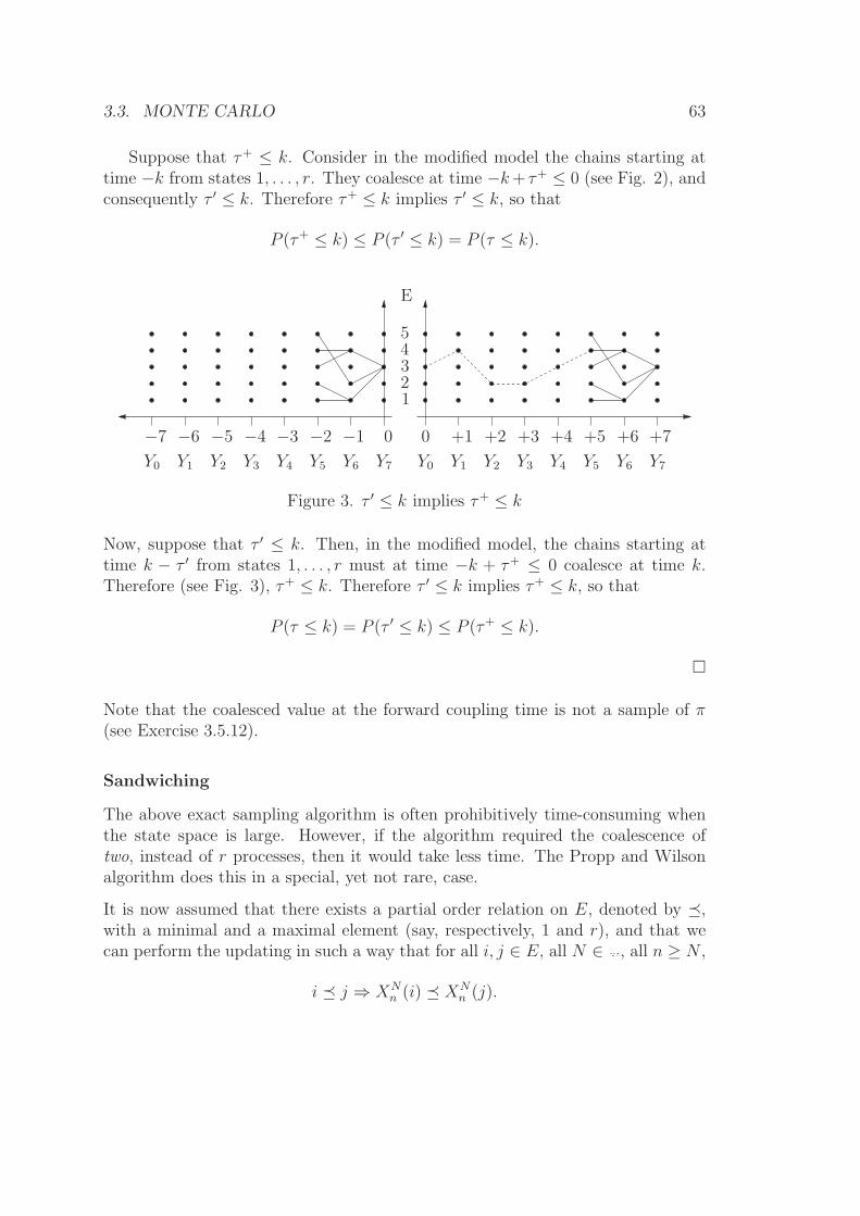
3.3. MONTE CARLO 63
Suppose that τ+ ≤ k. Consider in the modified model the chains starting attime −k from states 1, . . . , r. They coalesce at time −k+ τ+ ≤ 0 (see Fig. 2), andconsequently τ ′ ≤ k. Therefore τ+ ≤ k implies τ ′ ≤ k, so that
P (τ+ ≤ k) ≤ P (τ ′ ≤ k) = P (τ ≤ k).
00
12345
E
−1−2−3−4−5−6−7 +1 +2 +3 +4 +5 +6 +7
Y0 Y0Y1 Y1Y2 Y2Y3 Y3Y4 Y4Y5 Y5Y6 Y6 Y7Y7
Figure 3. τ ′ ≤ k implies τ+ ≤ k
Now, suppose that τ ′ ≤ k. Then, in the modified model, the chains starting attime k − τ ′ from states 1, . . . , r must at time −k + τ+ ≤ 0 coalesce at time k.Therefore (see Fig. 3), τ+ ≤ k. Therefore τ ′ ≤ k implies τ+ ≤ k, so that
P (τ ≤ k) = P (τ ′ ≤ k) ≤ P (τ+ ≤ k).
�
Note that the coalesced value at the forward coupling time is not a sample of π(see Exercise 3.5.12).
Sandwiching
The above exact sampling algorithm is often prohibitively time-consuming whenthe state space is large. However, if the algorithm required the coalescence oftwo, instead of r processes, then it would take less time. The Propp and Wilsonalgorithm does this in a special, yet not rare, case.
It is now assumed that there exists a partial order relation on E, denoted by �,with a minimal and a maximal element (say, respectively, 1 and r), and that wecan perform the updating in such a way that for all i, j ∈ E, all N ∈ , all n ≥ N ,
i � j ⇒ XNn (i) � XN
n (j).
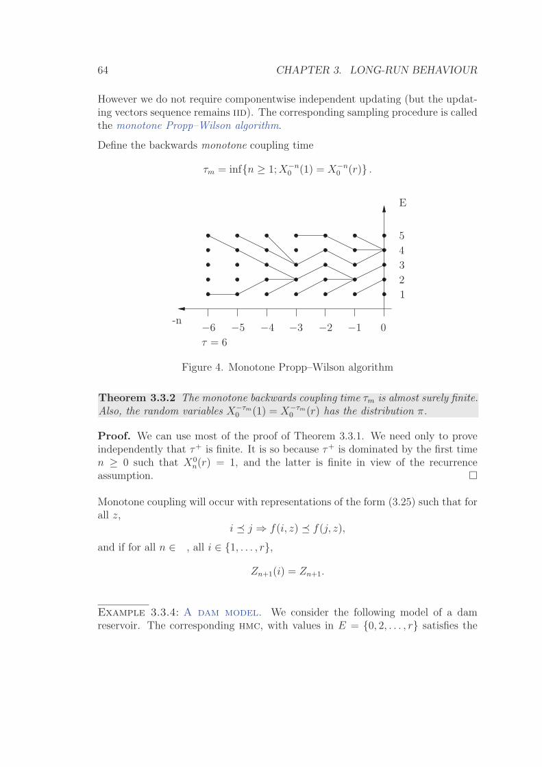
64 CHAPTER 3. LONG-RUN BEHAVIOUR
However we do not require componentwise independent updating (but the updat-ing vectors sequence remains iid). The corresponding sampling procedure is calledthe monotone Propp–Wilson algorithm.
Define the backwards monotone coupling time
τm = inf{n ≥ 1;X−n0 (1) = X−n
0 (r)} .
0
1
2
3
4
5
E
−1−2−3−4−5−6-n
τ = 6
Figure 4. Monotone Propp–Wilson algorithm
Theorem 3.3.2 The monotone backwards coupling time τm is almost surely finite.Also, the random variables X−τm
0 (1) = X−τm0 (r) has the distribution π.
Proof. We can use most of the proof of Theorem 3.3.1. We need only to proveindependently that τ+ is finite. It is so because τ+ is dominated by the first timen ≥ 0 such that X0
n(r) = 1, and the latter is finite in view of the recurrenceassumption. �
Monotone coupling will occur with representations of the form (3.25) such that forall z,
i � j ⇒ f(i, z) � f(j, z),
and if for all n ∈ , all i ∈ {1, . . . , r},
Zn+1(i) = Zn+1.
Example 3.3.4: A dam model. We consider the following model of a damreservoir. The corresponding hmc, with values in E = {0, 2, . . . , r} satisfies the
3.4. ABSORPTION 65
recurrence equation
Xn+1 = min{r,max(0, Xn + Zn+1)},
where, as usual, {Zn}n≥1 is iid. In this specific model, Xn is the content at timen of a dam reservoir with maximum capacity r, and Zn+1 = An+1− c, where An+1
is the input into the reservoir during the time period from n to n+1, and c is themaximum release during the same period. The updating rule is then monotone.
3.4 Absorption
Before absorption
We now consider the absorption problem for hmc’s based only on the transitionmatrix P, not necessarily assumed irreducible. The state space E is then decom-posable as E = T +
∑j Rj, where R1, R2, . . . are the disjoint recurrent classes and
T is the collection of transient states. (Note that the number of recurrent classesas well as the number of transient states may be infinite.) The transition matrixcan therefore be block-partitioned as
P =
P1 0 · · · 00 P2 · · · 0...
.... . .
...B(1) B(2) · · · Q
or in condensed notation,
P =
(D 0B Q
). (3.26)
This structure of the transition matrix accounts for the fact that one cannot gofrom a state in a given recurrent class to any state not belonging to this recurrentclass. In other words, a recurrent class is closed.
What is the probability of being absorbed by a given recurrent class when startingfrom a given transient state? This kind of problem was already addressed whenthe first-step analysis method was introduced. It led to systems of linear equationswith boundary conditions, for which the solution was unique, due to the finitenessof the state space. With an infinite state space, the uniqueness issue cannot beoverlooked, and the absorption problem will be reconsidered with this in mind,and also with the intention of finding general matrix-algebraic expressions for thesolutions. Another phenomenon not manifesting itself in the finite case is the
66 CHAPTER 3. LONG-RUN BEHAVIOUR
possibility, when the set of transient states is infinite, of never being absorbed bythe recurrent set. We shall consider this problem first, and then proceed to derivethe distribution of the time to absorption by the recurrent set, and the probabilityof being absorbed by a given recurrent class.
Let A be a subset of the state space E (typically the set of transient states, butnot necessarily). We aim at computing for any initial state i ∈ A the probabilityof remaining forever in A,
v(i) = Pi(Xr ∈ A; r ≥ 0).
Defining vn(i) := Pi(X1 ∈ A, . . . , Xn ∈ A), we have, by monotone sequentialcontinuity,
limn↑∞
↓ vn(i) = v(i).
But for j ∈ A, Pi(X1 ∈ A, . . . , Xn−1 ∈ A,Xn = j) =∑
i1∈A· · ·∑in−1∈A
pii1 · · · pin−1j
is the general term qij(n) of the n-th iterate of the restriction Q of P to the setA. Therefore vn(i) =
∑j∈A qij(n), that is, in vector notation,
vn = Qn1A,
where 1A is the column vector indexed by A with all entries equal to 1. From thisequality we obtain
vn+1 = Qvn,
and by dominated convergence v = Qv. Moreover, 0A ≤ v ≤ 1A, where 0A is thecolumn vector indexed by A with all entries equal to 0. The above result can berefined as follows:
Theorem 3.4.1 The vector v is the maximal solution of
v = Qv,0A ≤ v ≤ 1A.
Moreover, either v = 0A or supi∈Av(i) = 1. In the case of a finite transient set T ,the probability of infinite sojourn in T is null.
Proof. Only maximality and the last statement remain to be proven. To provemaximality consider a vector u indexed by A such that u = Qu and 0A ≤ u ≤ 1A.Iteration of u = Qu yields u = Qnu, and u ≤ 1A implies that Qnu ≤ Qn1A = vn.Therefore, u ≤ vn, which gives u ≤ v by passage to the limit.
To prove the last statement of the theorem, let c = supi∈A v(i). From v ≤ c1A, weobtain v ≤ cvn as above, and therefore, at the limit, v ≤ cv. This implies eitherv = 0A or c = 1.
3.4. ABSORPTION 67
When the set T is finite, the probability of infinite sojourn in T is null, becauseotherwise at least one transient state would be visited infinitely often. �
Equation v = Qv reads
v(i) =∑
j∈A
pijv(j) (i ∈ A) .
First-step analysis gives this equality as a necessary condition. However, it doesnot help to determine which solution to choose, in case there are several.
Example 3.4.1: The repair shop once more. We shall prove in a differentway a result already obtained in Subsection 2.4, that is: the chain is recurrent ifand only if ρ ≤ 1,. Observe that the restriction of P to Ai := {i + 1, i + 2, . . .},namely
Q =
a1 a2 a3 · · ·a0 a1 a2 · · ·
a0 a1 · · ·· · ·
,
does not depend on i ≥ 0. In particular, the maximal solution of v = Qv, 0A ≤ v ≤1A when A ≡ Ai has, in view of Theorem 3.4.1, the following two interpretations.Firstly, for i ≥ 1, 1− v(i) is the probability of visiting 0 when starting from i ≥ 1.Secondly, (1 − v(1)) is the probability of visiting {0, 1, . . . , i} when starting fromi + 1. But when starting from i + 1, the chain visits {0, 1, . . . , i} if and only if itvisits i, and therefore (1− v(1)) is also the probability of visiting i when startingfrom i+ 1. The probability of visiting 0 when starting from i+ 1 is
1− v(i+ 1) = (1− v(1))(1− v(i)),
because in order to go from i + 1 to 0 one must first reach i, and then go to 0.Therefore, for all i ≥ 1,
v(i) = 1− βi ,
where β = 1− v(1). To determine β, write the first equality of v = Qv:
v(1) = a1v(1) + a2v(2) + · · · ,
that is,(1− β) = a1(1− β) + a2(1− β2) + · · · .
Since∑
i≥0 ai = 1, this reduces to
β = g(β) , (⋆)
68 CHAPTER 3. LONG-RUN BEHAVIOUR
where g is the generating function of the probability distribution (ak, k ≥ 0). Also,all other equations of v = Qv reduce to (⋆).
Under the irreduciblity assumptions a0 > 0, a0 + a1 < 1, (⋆) has only one solutionin [0, 1], namely β = 1 if ρ ≤ 1, whereas if ρ > 1, it has two solutions in [0, 1],this probability is β = 1 and β = β0 ∈ (0, 1). We must take the smallest solution.Therefore, if ρ > 1, the probability of visiting state 0 when starting from statei ≥ 1 is 1− v(i) = βi
0 < 1, and therefore the chain is transient. If ρ ≤ 1, the latterprobability is 1− v(i) = 1, and therefore the chain is recurrent.
Example 3.4.2: 1-D random walk, take 5. The transition matrix of therandom walk on N with a reflecting barrier at 0,
P =
0 1q 0 p
q 0 pq 0 p
. . .
,
where p ∈ (0, 1), is clearly irreducible. Intuitively, if p > q, there is a drift to theright, and one expects the chain to be transient. This will be proven formally byshowing that the probability v(i) of never visiting state 0 when starting from statei ≥ 1 is strictly positive. In order to apply Theorem 3.4.1 with A = N − {0}, wemust find the general solution of u = Qu. This equation reads
u(1) = pu(2),
u(2) = qu(1) + pu(3),
u(3) = qu(2) + pu(4),
· · ·
and its general solution is u(i) = u(1)∑i−1
j=0
(qp
)j
. The largest value of u(1) re-
specting the constraint u(i) ∈ [0, 1] is u(1) = 1−(
qp
). The solution v(i) is therefore
v(i) = 1−(q
p
)i
.
3.4. ABSORPTION 69
Time to absorption
We now turn to the determination of the distribution of τ , the time of exit from thetransient set T . Theorem 3.4.1 tells that v = {v(i)}i∈T , where v(i) = Pi(τ = ∞),is the largest solution of v = Qv subject to the constraints 0T ≤ v ≤ 1T , whereQ is the restriction of P to the transient set T . The probability distribution of τwhen the initial state is i ∈ T is readily computed starting from the identity
Pi(τ = n) = Pi(τ ≥ n)− Pi(τ ≥ n+ 1)
and the observation that for n ≥ 1 {τ ≥ n} = {Xn−1 ∈ T}, from which we obtain,for n ≥ 1,
Pi(τ = n) = Pi(Xn−1 ∈ T )− P (Xn ∈ T ) =∑
j∈T
(pij(n− 1)− pij(n)).
Now, pij(n) is for i, j ∈ T the general term of Qn, and therefore:
Theorem 3.4.2
Pi(τ = n) = {(Qn−1 −Qn)1T}i . (3.27)
In particular, if Pi(τ = ∞) = 0,
Pi(τ > n) = {Qn1T}i .
Proof. Only the last statement remains to be proved. From (3.27),
Pi(n < τ ≤ n+m) =m−1∑
j=0
{(Qn+j −Qn+j−1)1T}i
={(
Qn −Qn+m)1T
}i,
and therefore, if Pi(τ = ∞) = 0, we obtain (3.27) by letting m ↑ ∞. �
Absorption destination
We seek to compute the probability of absorption by a given recurrent class whenstarting from a given transient state. As we shall see later, it suffices for the theoryto treat the case where the recurrent classes are singletons. We therefore supposethat the transition matrix has the form
P =
(I 0B Q
). (3.28)
70 CHAPTER 3. LONG-RUN BEHAVIOUR
Let fij be the probability of absorption by recurrent class Rj = {j} when startingfrom the transient state i. We have
Pn =
(I 0Ln Qn
),
where Ln = (I + Q + · · · + Qn)B. Therefore, limn↑∞ Ln = SB. For i ∈ T , the(i, j) term of Ln is
Ln(i, j) = P (Xn = j|X0 = i).
Now, if TRjis the first time of visit to Rj after time 0, then
Ln(i, j) = Pi(TRj≤ n),
since Rj is a closed state. Letting n go to ∞ gives the following:
Theorem 3.4.3 For a hmc with transition matrix P of the form (3.28), the prob-ability of absorption by recurrent class Rj = {j} starting from transient state i is
Pi(TRj<∞) = (SB)i,Rj
.
The general case, where the recurrence classes are not necessarily singletons, canbe reduced to the singleton case as follows. Let P∗ be the matrix obtained fromthe transition matrix P, by grouping for each j the states of recurrent class Rj
into a single state :
P∗ =
1 0 0 00 1 0 0
0 0. . . 0
b1 b2 · · · Q
(3.29)
where b = B(j)1T is obtained by summation of the columns of B(j), the matrixconsisting of the columns i ∈ Rj of B. The probability fiRj
of absorption by class
Rj when starting from i ∈ T equals fi, the probability of ever visiting whenstarting from i, computed for the chain with transition matrix P∗.
Example 3.4.3: Sibmating. In the reproduction model called sibmating (sister–brother mating), two individuals are mated and two individuals from their offspringare chosen at random to be mated, and this incestuous process goes on throughthe subsequent generations.
We shall denote by Xn the genetic type of the mating pair at the nth genera-tion. Clearly, {Xn}n≥0 is a hmc with six states representing the different pairsof genotypes AA × AA, aa × aa, AA × Aa, Aa × Aa, Aa × aa, AA × aa, de-noted respectively 1, 2, 3, 4, 5, 6. The following table gives the probabilities of
3.4. ABSORPTION 71
occurrence of the 3 possible genotypes in the descent of a mating pair:
AA AAaa aaAA AaAa AaAa aaAA aa
AA Aa aa1 0 00 0 11/2 1/2 01/4 1/2 1/40 1/2 1/20 1 0
parents’ genotype
︷ ︸︸ ︷descendant’s genotype
The transition matrix of {Xn}n≥0 is then easily deduced:
P =
11
1/4 1/2 1/41/16 1/16 1/4 1/4 1/4 1/8
1/4 1/4 1/21
.
The set R = {1, 2} is absorbing, and the restriction of the transition matrix to thetransient set T = {3, 4, 5, 6} is
Q =
1/2 1/4 0 01/4 1/4 1/4 1/80 1/4 1/2 00 1 0 0
.
We find
S = (1−Q)−1 =1
6
16 8 4 18 16 8 24 8 16 18 16 8 8
,
and the absorption probability matrix is
SB = S
1/4 01/16 1/160 1/40 0
=
3/4 1/41/2 1/21/4 3/41/2 1/2
.
For instance, the (3, 2)entry, 34, is the probability that when starting from a couple
of ancestors of type Aa × aa, the race will end up in genotype aa × aa.
72 CHAPTER 3. LONG-RUN BEHAVIOUR
3.5 Exercises
Exercise 3.5.1. abbabaa!A sequence of A’s and B’s is formed as follows. The first item is chosen at random,P (A) = P (B) = 1
2, as is the second item, independently of the first one. When
the first n ≥ 2 items have been selected, the (n+ 1)st is chosen, independently ofthe letters in positions k ≤ n − 2 conditionally on the pair at position n − 1 andn, as follows:
P (A | AA) = 1
2, P (A | AB) =
1
2, P (A | BA) = 1
4, P (A | BB) =
1
4.
What is the proportion of A’s and B’s in a long chain?
Exercise 3.5.2. Fixed-age retirement policy.Let {Un}n≥1 be a sequence of iid random variables taking their values in + ={1, 2, . . . , }. The random variable Un is interpreted as the lifetime of some equip-ment, or “machine”, the nth one, which is replaced by the (n + 1)st one uponfailure. Thus at time 0, machine 1 is put in service until it breaks down at timeU1, whereupon it is immediately replaced by machine 2, which breaks down attime U1+U2, and so on. The time to next failure of the current machine at time nis denoted by Xn. More precisely, the process {Xn}n≥0 takes its values in E = N,
equals 0 at time Rk =∑k
i=1 Ui, equals Uk+1−1 at time Rk+1, and then decreasesof one unit per unit of ime until it reaches the value 0 at time Rk+1. It is assumedthat for all k ∈ +, P (U1 > k) > 0, so that the state space E is . Then {Xn}n≥0
is an irreducible hmc called thr forward recurrence chain. We assume positiverecurrence, that is E[U ] <∞, where U = U1.
A. Show that the chain is irreducible. Give the necessary and sufficient conditionfor positive recurrence. Assuming positive recurrence, what is the stationary dis-tribution? A visit of the chain to state 0 corresponds to a breakdown of a machine.What is the empirical frequency of breakdowns?
B. Suppose that the cost of a breakdown is so important that it is better to replacea working machine during its lifetime (breakdown implies costly repairs, whereasreplacement only implies moderate maintenance costs). The fixed-age retirementpolicy fixes an integer T ≥ 1 and requires that a machine having reached age Tbe immediately replaced. What is the empirical frequency of breakdowns (notreplacements)?
Exercise 3.5.3. Convergence speed via coupling.Suppose that the coupling time τ in Theorem 3.2.3 satisfies
E[ψ(τ)] <∞
3.5. EXERCISES 73
for some non-decreasing function ψ : N → R+ such that limn↑∞ ψ(n) = ∞. Showthat for any initial distributions µ and ν
|µTPn − νTPn| = o
(1
ψ(n)
).
Exercise 3.5.4.Let {Zn}n≥1 be an iid sequence of iid {0, 1}-valued random variables, P (Zn =1) = p ∈ (0, 1). Show that for all k ≥ 1,
limn↑∞
P (Z1 + Z2 + · · ·Zn is divisible by k) = 1 .
Hint: modulo k.
Exercise 3.5.5.Let P be an ergodic transition matrix on the finite state space E. Prove thatfor any initial distributions µ and ν, one can construct two hmc’s {Xn}n≥0 and{Yn}n≥0 on E with the same transition matrix P, and the respective initial dis-tributions µ and ν, in such a way that they couple at a finite time τ such thatE[eατ ] <∞ for some α > 0.
Exercise 3.5.6. The lazy random walk on the circle.Consider N points on the circle forming the state space E := {0, 1, . . . , N − 1}.Two points i, j are said to be neighbours if j = i ± 1 modulo n. Consider theMarkov chain {(Xn, Yn)}n≥0 with state space E×E and representing two particlesmoving on E as follows. At each time n choose Xn or Yn with probability 1
2and
move the corresponding particle to the left or to the right, equiprobably whilethe other particle remains still. The initial positions of the particles are a and brespectively. Compute the average time it takes until the two particles collide (theaverage coupling time of two lazy random walks).
Exercise 3.5.7. Coupling time for the 2-state hmc.Find the distribution of the first meeting time of two independent hmc with statespace E = {1, 2} and transition matrix
P =
(1− α αβ 1− β
),
where α, β ∈ (0, 1), when their initial states are different.
Exercise 3.5.8. The snake chain.
74 CHAPTER 3. LONG-RUN BEHAVIOUR
Let {Xn}n≥0 be an hmc with state space E and transition matrix P. Define forL ≥ 1, Yn = (Xn, Xn+1, . . . , Xn+L).
(a) The process {Yn}n≥0 takes its values in F = EL+1. Prove that {Yn}n≥0 is anhmc and give the general entry of its transition matrix. (The chain {Yn}n≥0 iscalled the snake chain of length L+ 1 associated with {Xn}n≥0.)
(b) Show that if {Xn}n≥0 is irreducible, then so is {Yn}n≥0 if we restrict the statespace of the latter to be F = {(i0, . . . , iL) ∈ EL+1; pi0i1pi1i2 · · · piL−1iL > 0}. Showthat if the original chain is irreducible aperiodic, so is the snake chain.
(c) Show that if {Xn}n≥0 has a stationary distribution π, then {Yn}n≥0 also has astationary distribution. Which one?
Exercise 3.5.9. Target time.Let π be the stationary distribution of an ergodic Markov chain with finite statespace, and denote by Ti the return time to state i. Let SZ be the time necessaryto visit for the first time the random state Z chosen according to the distributionπ, independently of the chain. Show that Ei[SZ ] is independent of i, and give itsexpression in terms of the fundamental matrix.
Exercise 3.5.10. Mean time between successive visits of a set.Let {Xn}n≥0 be an irreducible positive recurrent hmc with stationary distributionπ. Let A be a subset of the state space E and let {τ(k)}k≥1 be the sequence ofreturn times to A. Show that
limk↑∞
τ(k)
k=
1∑i∈A π(i)
.
(This extends Formula (2.5)).
Exercise 3.5.11. Irreducibility of the Barker sampling chain.Show that for both the Metropolis and Barker samplers, if Q is irreducible and Uis not a constant, then P(T ) is irreducible and aperiodic for all T > 0.
Exercise 3.5.12. Forward coupling does not yield exact sampling.Refer to the Propp–Wilson algorithm. Show that the coalesced value at the for-wards coupling time is not a sample of π. For a counterexample use the two-statehmc with E = {1, 2}, p1,2 = 1, p2,2 = p2,1 = 1/2.
Exercise 3.5.13. The modified random walk.Consider the usual random walk on a graph. Its stationary distribution is ingeneral non-uniform. We wish to modify it so as to obtain a hmc with uniform
3.5. EXERCISES 75
stationary distribution. Now accept a transition from vertex i to vertex j of theoriginal random walk with probability αij . Find one such acceptance probabilitydepending only d(i) and d(j) that guarantees that the corresponding Monte CarloMarkov chain admits the uniform distribution as stationary distribution.


![A Compositional Framework for Markov Processesmath.ucr.edu/home/baez/markov.pdf · At least since the work of Prigogine [9,20], it is widely accepted that a large class of systems](https://static.documents.pub/doc/80x56/5bcab8e709d3f241138d2a52/a-compositional-framework-for-markov-at-least-since-the-work-of-prigogine-920.jpg)


