Page 1
S.V.N. “Vishy” Vishwanathan: Basic Mathematics, Page 1
Basic MathematicsA Machine Learning Perspective
S.V.N. “Vishy” [email protected]
National ICT of Australiaand
Australian National University
Thanks to Alex Smola for intial version of slides
Page 2
Overview
S.V.N. “Vishy” Vishwanathan: Basic Mathematics, Page 2
Functional Analysis
Linear Algebra
Matrix Theory
Probability
Page 3
Metric Spaces
S.V.N. “Vishy” Vishwanathan: Basic Mathematics, Page 3
Metric Space:A pair (X, d), where X is a set and d : X×X → R+
0 is ametric space if ∀x,y, z ∈ X
d(x,y) = 0 iff x = y
d(x,y) = d(y,x) (Symmetry )d(x, z) ≤ d(x,y) + d(y, z) (Triangle inequality )
Examples:Euclidean space
For all x,y ∈ Rn we define d(x,y) =√∑n
i=1(xi − yi)2
`p-spaceSpace of sequences with d(x,y) = (
∑∞i=1 |xi − yi|p)
1p
Hilbert spaceSpace of sequences with d(x,y) =
√∑∞i=1(xi − yi)2
Page 4
Balls, Open and Closed Sets
S.V.N. “Vishy” Vishwanathan: Basic Mathematics, Page 4
Ball:Given x0 ∈ X and r > 0 we define
B(x0, r) = {x ∈ X |d(x,x0) < r} (Open ball)B(x0, r) = {x ∈ X |d(x,x0) ≤ r} (Closed ball)
Open set:A subset M of a metric space X is open if it contains anopen ball about each of its points
Closed set:If the complement of M is open it is called a closed set
Examples:The set (a, b) ⊂ R is an open setThe set [a, b] ⊂ R is a closed setThe set (a, b] ⊂ R is neither open nor closed
Page 5
Cauchy Sequences
S.V.N. “Vishy” Vishwanathan: Basic Mathematics, Page 5
Convergence:A sequence {xi} ∈ X is said to converge if for any ε thereexists a x and a n0 such that for all n ≥ n0 we haved(xn, x) ≤ ε
Cauchy Series:A sequence {xi} ∈ X is a Cauchy if for any ε there existsa n0 such that for all m, n ≥ n0 we have d(xm,xn) ≤ ε
Completeness:A space X is complete if the limits of every Cauchy se-ries are elements of X
We call X̄ the completion of X, i.e. the union of X andthe limits of all Cauchy series in X
The real line R and complex plane C are completeThe set Q of rationals is not complete!
Page 6
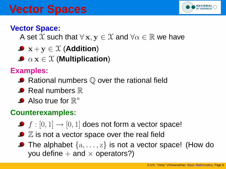
Vector Spaces
S.V.N. “Vishy” Vishwanathan: Basic Mathematics, Page 6
Vector Space:A set X such that ∀x,y ∈ X and ∀α ∈ R we have
x+y ∈ X (Addition )αx ∈ X (Multiplication )
Examples:Rational numbers Q over the rational fieldReal numbers RAlso true for Rn
Counterexamples:
f : [0, 1] → [0, 1] does not form a vector space!Z is not a vector space over the real fieldThe alphabet {a, . . . , z} is not a vector space! (How doyou define + and × operators?)
Page 7
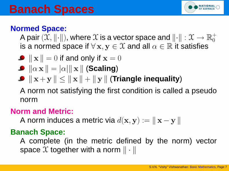
Banach Spaces
S.V.N. “Vishy” Vishwanathan: Basic Mathematics, Page 7
Normed Space:A pair (X, ‖·‖), where X is a vector space and ‖·‖ : X → R+
0is a normed space if ∀x,y ∈ X and all α ∈ R it satisfies
‖x ‖ = 0 if and only if x = 0
‖αx ‖ = |α|‖x ‖ (Scaling )‖x+y ‖ ≤ ‖x ‖ + ‖y ‖ (Triangle inequality )
A norm not satisfying the first condition is called a pseudonorm
Norm and Metric:A norm induces a metric via d(x,y) := ‖x−y ‖
Banach Space:A complete (in the metric defined by the norm) vectorspace X together with a norm ‖ · ‖
Page 8
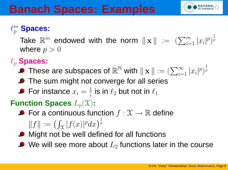
Banach Spaces: Examples
S.V.N. “Vishy” Vishwanathan: Basic Mathematics, Page 8
`mp Spaces:
Take Rm endowed with the norm ‖x ‖ := (∑m
i=1 |xi|p)1p
where p > 0
`p Spaces:These are subspaces of RN with ‖x ‖ := (
∑∞i=1 |xi|p)
1p
The sum might not converge for all seriesFor instance xi = 1
i is in `2 but not in `1
Function Spaces Lp(X):For a continuous function f : X → R define
‖f‖ :=(∫
X|f (x)|pdx
)1p
Might not be well defined for all functionsWe will see more about L2 functions later in the course
Page 9
Hilbert Spaces
S.V.N. “Vishy” Vishwanathan: Basic Mathematics, Page 9
Inner Product Space:A pair (X, ‖ · ‖), where X is a vector space and〈·, ·〉 : X×X → R+
0 is a inner product space if ∀x,y z ∈ Xand all α ∈ R it satisfies
〈x+y, z〉 = 〈x, z〉 + 〈y, z〉 (Additivity )〈αx,y〉 = α〈x,y〉 (Linearity )〈x,y〉 = 〈y,x〉 (Symmetry )〈x,x〉 = 0 ⇐⇒ x = 0
Dot Product and Norm:A dot product induces a norm via ‖x ‖ :=
√〈x,x〉
Hilbert Space:A complete (in the metric induced by the dot product) vec-tor space X, endowed with a dot product 〈·, ·〉
Page 10
Hilbert Spaces: Examples
S.V.N. “Vishy” Vishwanathan: Basic Mathematics, Page 10
Euclidean Spaces:Take Rm endowed with the dot product 〈x,y〉 :=
∑mi=1 xiyi
`2 Spaces:Infinite series of real numbersWe define a dot product as 〈x,y〉 =
∑∞i=1 xiyi
Function Spaces L2(X):For continuous functions f, g : X → C define〈f, g〉 :=
∫X f (x)g(x)dx
We take the complex conjugate of f and replace thesum by an integral
Polarization Inequality:To recover the dot product from the norm compute‖x+y ‖2 − ‖x ‖2 − ‖y ‖2 = 2〈x,y〉
Page 11
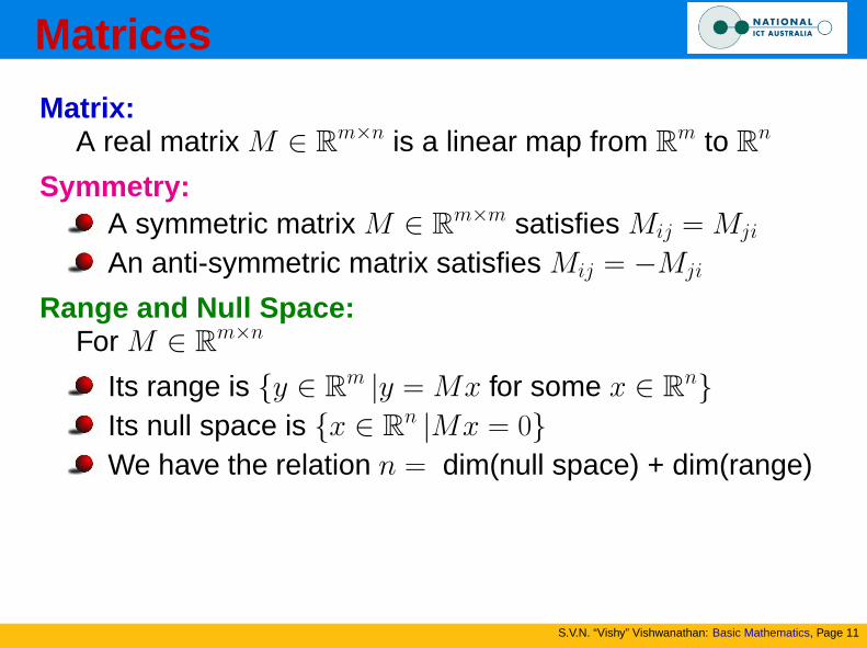
Matrices
S.V.N. “Vishy” Vishwanathan: Basic Mathematics, Page 11
Matrix:A real matrix M ∈ Rm×n is a linear map from Rm to Rn
Symmetry:A symmetric matrix M ∈ Rm×m satisfies Mij = Mji
An anti-symmetric matrix satisfies Mij = −Mji
Range and Null Space:For M ∈ Rm×n
Its range is {y ∈ Rm |y = Mx for some x ∈ Rn}Its null space is {x ∈ Rn |Mx = 0}We have the relation n = dim(null space) + dim(range)
Page 12
Rank
S.V.N. “Vishy” Vishwanathan: Basic Mathematics, Page 12
Definition:If M ∈ Rm×n, rank M is the largest number of columns ofM that constitute a linearly independent set
Characteristics:The following are equivalent for a rank k matrix M
Exactly k rows (columns) of M are linearly independentDimension of range of M is is k
∃ a k-by-k sub-matrix of M with non-zero determinantAll (k + 1)-by-(k + 1) sub-matrices have determinant 0
Properties:For M ∈ Rm×n, rank(M) ≤ min{m, n}Deleting rows/columns can only decrease the rankFor M, N ∈ Rm×n, rank(M + N) ≤ rank(M) + rank(N)
Page 13
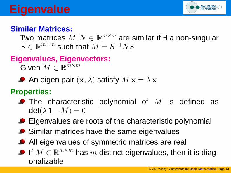
Eigenvalue
S.V.N. “Vishy” Vishwanathan: Basic Mathematics, Page 13
Similar Matrices:Two matrices M, N ∈ Rm×m are similar if ∃ a non-singularS ∈ Rm×m such that M = S−1NS
Eigenvalues, Eigenvectors:Given M ∈ Rm×m
An eigen pair (x, λ) satisfy M x = λx
Properties:The characteristic polynomial of M is defined asdet(λ1−M) = 0
Eigenvalues are roots of the characteristic polynomialSimilar matrices have the same eigenvaluesAll eigenvalues of symmetric matrices are realIf M ∈ Rm×m has m distinct eigenvalues, then it is diag-onalizable
Page 14
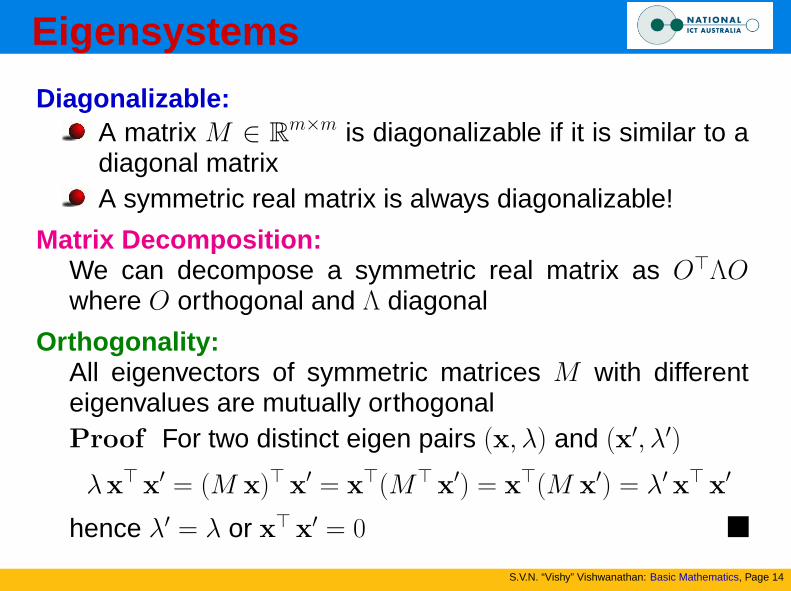
Eigensystems
S.V.N. “Vishy” Vishwanathan: Basic Mathematics, Page 14
Diagonalizable:A matrix M ∈ Rm×m is diagonalizable if it is similar to adiagonal matrixA symmetric real matrix is always diagonalizable!
Matrix Decomposition:We can decompose a symmetric real matrix as O>ΛOwhere O orthogonal and Λ diagonal
Orthogonality:All eigenvectors of symmetric matrices M with differenteigenvalues are mutually orthogonalProof For two distinct eigen pairs (x, λ) and (x′, λ′)
λx> x′ = (M x)> x′ = x>(M> x′) = x>(M x′) = λ′ x> x′
hence λ′ = λ or x> x′ = 0
Page 15
Orthogonality
S.V.N. “Vishy” Vishwanathan: Basic Mathematics, Page 15
Orthonormal Set:A set {x1,x2, . . . ,xn} is orthonormal if 〈xi,xj〉 = 0 if i 6= jand ‖xi ‖ = 1 for all i
Orthogonal Matrix:An orthogonal matrix M ∈ Rm×m is made up of or-thonormal rows and columnsNot difficult to see that MM> = 1
Equivalently M−1 = M>
Properties:Orthogonal transformations preserve matrix norms
Page 16
Matrix Invariants
S.V.N. “Vishy” Vishwanathan: Basic Mathematics, Page 16
Trace:Trace is the sum of the diagonal elementsFor symmetric matrices tr(MN) = tr(NM)
Orthogonal matrices preserve trace sincetr(O>MO) = tr(MOO>) = trM
It can be shown that tr(M) =∑m
i=1 λi
Determinant:Antisymmetric multi-linear form, i.e. swapping columns orrows changes the sign, adding elements in rows andcolumns is linear. Useful form
detM =
m∏i=1
λi
Invariant under orthogonal transformations
Page 17
Matrix Norms
S.V.N. “Vishy” Vishwanathan: Basic Mathematics, Page 17
Definition:We call a function ‖ · ‖ : Rm×m → R+
0 a matrix norm if forall M, N ∈ Rm×m we have
‖M‖ = 0 iff M = 0
‖cM‖ = |c|‖M‖ for all c ∈ R‖M + N‖ = ‖M‖ + ‖N‖‖MN‖ = ‖M‖‖N‖ (Cauchy Schwartz?)
Matrix norms are closely related to the eigenvalues of thematrix (more on this later)
Examples:The `1 norm is defined as ‖M‖1 :=
∑mi,j=1 |mij|
The `2 norm is defined as ‖M‖1 :=(∑m
i,j=1 m2ij
)12
Page 18
Matrix Norms Revisited
S.V.N. “Vishy” Vishwanathan: Basic Mathematics, Page 18
Operator Norm: Using M ∈ Rm×m we have
‖M‖2 = maxx∈Rm
‖M x ‖2
‖x ‖2
= maxx∈Rm and ‖x ‖=1
‖M x ‖2
= maxx∈Rm and ‖x ‖=1
x>OΛO>OΛO x
= maxx′∈Rm and ‖x′ ‖=1
x′>Λ2 x′
= maxi∈[m]
λ2i .
Frobenius Norm:Likewise we obtain ‖M‖2
Frob = trOΛO>OΛO> = trΛ2 =∑mi=1 λ2
i
Page 19
Positive Matrices
S.V.N. “Vishy” Vishwanathan: Basic Mathematics, Page 19
Positive Definite Matrix:A matrix M ∈ Rm×m for which for all x ∈ Rm we have
x>M x ≥ 0 if x 6= 0
This matrix has only positive eigenvalues since for alleigenvectors x we have x>M x = λx> x = λ‖x ‖2 > 0and thus λ > 0.
Induced Norms and Metrics:Every positive definite matrix induces a norm via
‖x ‖2M := x>M x
The triangle inequality can be seen by writing
‖x+x′ ‖2M = (x+x′)>M
12M
12(x+x′) = ‖M
12(x+x′)‖2
and using the triangle inequality for M12 x and M
12 x′.
Page 20
Singular Value Decompositions
S.V.N. “Vishy” Vishwanathan: Basic Mathematics, Page 20
Idea:Can we find something similar to the eigenvalue / eigen-vector decomposition for arbitrary matrices?
Decomposition:Without loss of generality assume m ≥ n For M ∈ Rm×n
we may write M as UΛO where U ∈ Rm×n, O ∈ Rn×n, andΛ = diag(λ1, . . . , λn).Furthermore O>O = OO> = U>U = 1.
Useful Trick:Nonzero eigenvalues of M>M and MM> are the same.This is so since M>M x = λx and hence (MM>)M x =λM x or equivalently (MM>)x′ = λx′
Page 21
Probability
S.V.N. “Vishy” Vishwanathan: Basic Mathematics, Page 21
Basic Idea:We have events, denoted by sets X ⊂ X in a space ofpossible outcomes X. Then P(X) tells us how likely is thatan event x with x ∈ X will occur.
Basic Axioms:
Pr(X) ∈ [0, 1] for all X ⊆ X
Pr(X) = 1
Pr (∪iXi) =∑
i
Pr(Xi) if Xi ∩Xj = ∅ for all i 6= j
I am hiding gory details about σ-algebra on X here
Simple Corollary:
Pr(Xi ∪Xj) = Pr(Xi) + Pr(Xj)− Pr(Xi ∩Xj)
Page 22
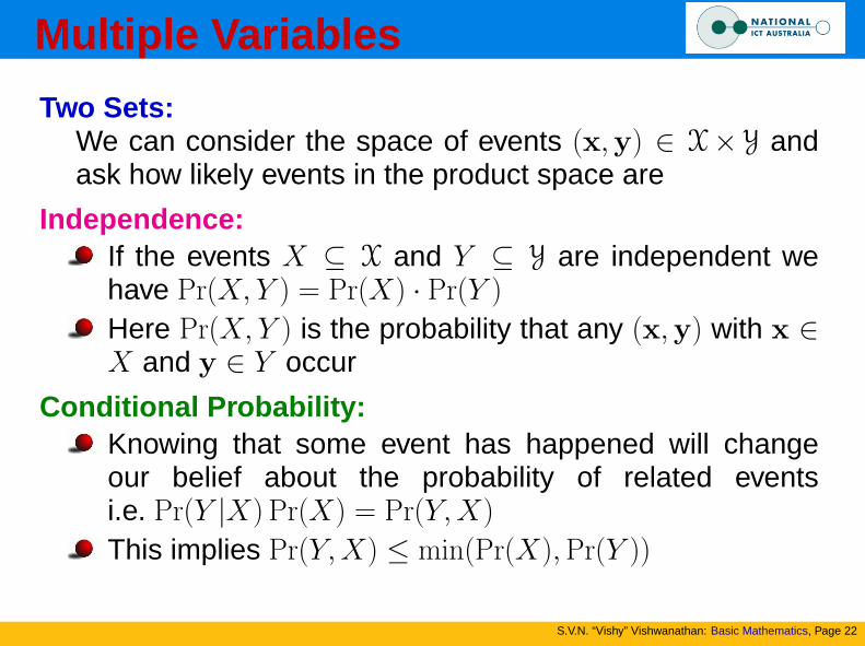
Multiple Variables
S.V.N. “Vishy” Vishwanathan: Basic Mathematics, Page 22
Two Sets:We can consider the space of events (x,y) ∈ X×Y andask how likely events in the product space are
Independence:If the events X ⊆ X and Y ⊆ Y are independent wehave Pr(X,Y ) = Pr(X) · Pr(Y )
Here Pr(X,Y ) is the probability that any (x,y) with x ∈X and y ∈ Y occur
Conditional Probability:Knowing that some event has happened will changeour belief about the probability of related eventsi.e. Pr(Y |X) Pr(X) = Pr(Y, X)
This implies Pr(Y, X) ≤ min(Pr(X), Pr(Y ))
Page 23
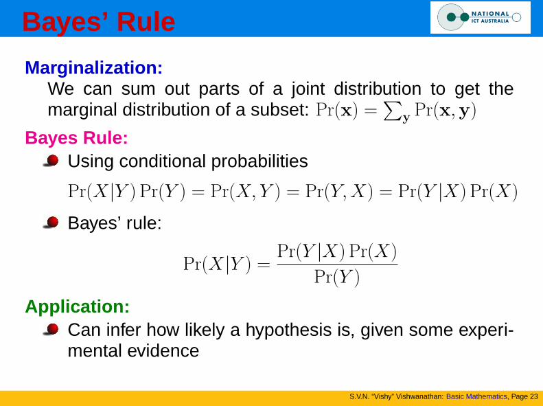
Bayes’ Rule
S.V.N. “Vishy” Vishwanathan: Basic Mathematics, Page 23
Marginalization:We can sum out parts of a joint distribution to get themarginal distribution of a subset: Pr(x) =
∑y Pr(x,y)
Bayes Rule:Using conditional probabilities
Pr(X|Y ) Pr(Y ) = Pr(X,Y ) = Pr(Y,X) = Pr(Y |X) Pr(X)
Bayes’ rule:
Pr(X|Y ) =Pr(Y |X) Pr(X)
Pr(Y )
Application:Can infer how likely a hypothesis is, given some experi-mental evidence
Page 24
Example - I
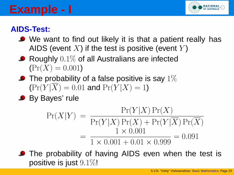
S.V.N. “Vishy” Vishwanathan: Basic Mathematics, Page 24
AIDS-Test:We want to find out likely it is that a patient really hasAIDS (event X) if the test is positive (event Y )Roughly 0.1% of all Australians are infected(Pr(X) = 0.001)The probability of a false positive is say 1%(Pr(Y |X) = 0.01 and Pr(Y |X) = 1)By Bayes’ rule
Pr(X|Y ) =Pr(Y |X) Pr(X)
Pr(Y |X) Pr(X) + Pr(Y |X) Pr(X)
=1× 0.001
1× 0.001 + 0.01× 0.999= 0.091
The probability of having AIDS even when the test ispositive is just 9.1%!
Page 25
Example - II
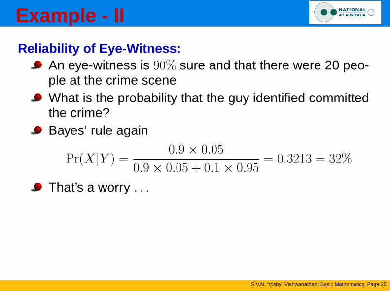
S.V.N. “Vishy” Vishwanathan: Basic Mathematics, Page 25
Reliability of Eye-Witness:An eye-witness is 90% sure and that there were 20 peo-ple at the crime sceneWhat is the probability that the guy identified committedthe crime?Bayes’ rule again
Pr(X|Y ) =0.9× 0.05
0.9× 0.05 + 0.1× 0.95= 0.3213 = 32%
That’s a worry . . .
Page 26
Densities:
S.V.N. “Vishy” Vishwanathan: Basic Mathematics, Page 26
Computing Pr(X):If we deal with continuous valued X we need integrals.
Pr(X) :=
∫X
d Pr(x) =
∫X
p(x)dx
Note that the last equality only holds if such a p(x) exists.For the rest of this course we assume that such a p exists. . .
Page 27
Bayes’ Rule for Densities
S.V.N. “Vishy” Vishwanathan: Basic Mathematics, Page 27
Multivariate Densities:Densities on product spaces (X×Y) are given by p(x,y)
Conditional Densities:For independent variables the densities factorize and wehave
p(x,y) = p(x)p(y)
For dependent variables (i.e. x tells us something about yand vice versa) we obtain
p(x,y) = p(x |y)p(y) = p(y |x)p(x)
Bayes’ Rule:Solving for p(y |x) yields
p(y |x) =p(x |y)p(y)
p(x)
Page 28
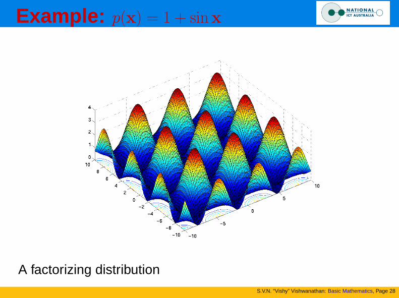
Example: p(x) = 1 + sinx
S.V.N. “Vishy” Vishwanathan: Basic Mathematics, Page 28
A factorizing distribution
Page 29
Random Variables
S.V.N. “Vishy” Vishwanathan: Basic Mathematics, Page 29
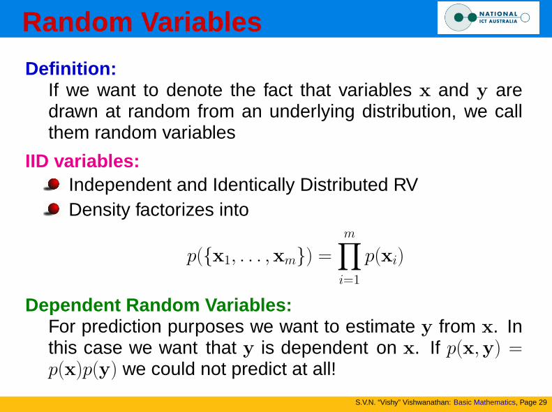
Definition:If we want to denote the fact that variables x and y aredrawn at random from an underlying distribution, we callthem random variables
IID variables:Independent and Identically Distributed RVDensity factorizes into
p({x1, . . . ,xm}) =
m∏i=1
p(xi)
Dependent Random Variables:For prediction purposes we want to estimate y from x. Inthis case we want that y is dependent on x. If p(x,y) =p(x)p(y) we could not predict at all!
Page 30
Marginalization
S.V.N. “Vishy” Vishwanathan: Basic Mathematics, Page 30
Marginalization:Given p(x,y) we can integrate out y to obtain p(x) via
p(x) =
∫Y
p(x,y)dy
Conditioning:If we know y, we can obtain p(x |y) via Bayes rule, i.e.
p(x |y) =p(y |x)p(x)
p(y)=
p(x,y)
p(y).
A similar trick, however, is to note that the dependence ofthe RHS on x lies only in p(x,y) and therefore we obtain
p(x |y) =p(x,y)∫
Xp(x,y)dx
Page 31
Expectation
S.V.N. “Vishy” Vishwanathan: Basic Mathematics, Page 31
Definition:The expectation of a function f (x) with respect to the ran-dom variable x is defined as
Ex[f (x)] :=
∫X
f (x)d Pr(x) =
∫X
f (x)p(x)dx
The last equation is valid if a density exists
Intuition:It is the mean value we get by sampling a large numberof x according to p(x) and evaluating f (x) on the drawnsample
Other Facts:Moments are expectations of higher ordersKnowledge of all the moments completely determinesthe distribution
Page 32
Examples
S.V.N. “Vishy” Vishwanathan: Basic Mathematics, Page 32
Uniform Distribution:Assume the uniform distribution on [0, 10]. What is the ex-pected value of f (x) = x2?
Ex[f (x)] =
∫[0,10]
f (x)p(x)dx =
∫[0,10]
x2 1
10dx = 33
1
3
Roulette:What is the expected loss in roulette when we bet on anumber, say j (we win 36$:1$ if the number is hit and 0$:1$otherwise)?
Ex[f (x)] =
37∑i=1,i 6=j
−1$ · 1
37+ 35$ · 1
37= − 1
37$
Page 33
Mean and Mode
S.V.N. “Vishy” Vishwanathan: Basic Mathematics, Page 33
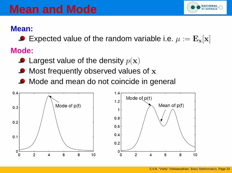
Mean:Expected value of the random variable i.e. µ := Ex[x]
Mode:Largest value of the density p(x)
Most frequently observed values of xMode and mean do not coincide in general
Page 34
Variance
S.V.N. “Vishy” Vishwanathan: Basic Mathematics, Page 34
Definition:Amount of variation in the random variableFirst center and then compute second order moment
σ2 := Ex
[(x−Ex[x])2
]= Ex x2− (Ex[x])2
Normalization:Rescale data to zero mean and unit variancePreprocess data by x → x−µ
σ
Tails of Distributions:Note that the variance need not always existTails of distributions give an idea about how sharply con-centrated the distribution is around its meanLong-tailed distributions can be killers for insurancecompanies!
Page 35
Markov’s Inequality
S.V.N. “Vishy” Vishwanathan: Basic Mathematics, Page 35
Markov’s Inequality:If x takes only non-negative values then
Pr(x ≥ a) ≤ E[x]/a
Proof:We write
E[x] =
∫ a
0
x p(x)dx+
∫ ∞
a
x p(x)dx
≥∫ ∞
a
x p(x)dx non-negativity
≥ a
∫ ∞
a
p(x)dx = a Pr(x ≥ a)
Observation:Completely independent of the distribution!
Page 36
Chebyshev’s Inequality
S.V.N. “Vishy” Vishwanathan: Basic Mathematics, Page 36
Chebyshev’s Inequality:For any random variable x we can bound deviations of xfrom its mean E[x] by
Pr(|x−E[x]| > C) ≤ σ2
C2
Proof:Apply Markov’s inequality to y := (x−E[x])2
Applications:Information about some measurement is easy to getEasy to estimate the variance tooDon’t know anything about the distribution :-(Still can make statements about probability of deviatingfrom the mean!
Page 37
Jensen’s Inequality
S.V.N. “Vishy” Vishwanathan: Basic Mathematics, Page 37
Jensens’s Inequality:If f is a convex function and X is a random variable then
E[f (X)] ≥ f (E[X ])
Picture:Notice how expectation is a linear operator
Page 38
Entropy
S.V.N. “Vishy” Vishwanathan: Basic Mathematics, Page 38
Definition:Measures the disorder of a systemDefined as
H(p) = −∑x
p(x) log p(x)
Properties:H(p) > 0 unless only one possible outcomeMaximal value occurs for uniform p
Deep connections to information theory exist
Page 39
Normal Distribution
S.V.N. “Vishy” Vishwanathan: Basic Mathematics, Page 39
The Formula:
p(x) =1√
2πσ2e−
(x−µ)2
2σ2
Mean:Notice that p(µ + ξ) = p(µ− ξ) because ((µ + ξ)− µ)2 =ξ2 = ((µ− ξ)− µ)2
Hence the mean of p(x) is µ
Variance:The variance of p(x) is σ2. We show this by proving that
Varx =
∫R
p(x)(x− µ)2dx =
∫R
p(µ + ξ)ξ2dξ
= σ2 1√2π
∫R
e−ξ22 ξ2dξ = σ2
Page 40
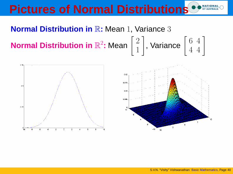
Pictures of Normal Distributions
S.V.N. “Vishy” Vishwanathan: Basic Mathematics, Page 40
Normal Distribution in R: Mean 1, Variance 3
Normal Distribution in R2: Mean
[21
], Variance
[6 44 4
]
Page 41
Covariance and Correlation
S.V.N. “Vishy” Vishwanathan: Basic Mathematics, Page 41
Covariance:For a multivariate distribution
Cov x := E[(x−µ)(x−µ)>
]We now compute a matrix instead of a single numberIn particular
(Cov x)ij = E [(xi − µi)(xi − µi)]
Correlated Variables:Measures degree of association between variablesIf positively correlated then
(Cov x)ij =√
(Cov x)ii (Cov x)jj
For uncorrelated variables their covariance vanishes
Page 42
Multivariate Normal
S.V.N. “Vishy” Vishwanathan: Basic Mathematics, Page 42
The Formula:Σ ∈ Rm×m is positive definiteThe mean µ ∈ Rm
p(x) =1√
(2π)mdetΣexp
(−1
2(x−µ)>Σ−1(x−µ)
)Mean:
Obviously this is µ (we can check that by symmetry)
Variance:Tedious calculation shows that Var(x) = Σ
Hint: decompose Σ = O>ΛO
Hint: use detΣ = detOΣO> =∏
i λi, where λi are theeigenvalues of Σ
Page 43
Laplacian Distribution - I
S.V.N. “Vishy” Vishwanathan: Basic Mathematics, Page 43
Decay of Atoms:The probability that a atom decays within 1 sec is 1− p
The probability that it decays in n sec is 1− pn
In the continuous domain the probability of decay aftertime T is
P (ξ ≤ T ) = 1− exp(−λT ) =
∫ T
0
p(t)dt
Laplacian Distribution:Consequently, p(t) is given by λ exp(−λT )
It is a particularly long-tailed distribution
Mean and Variance:Mean is given by µ = 1
λ
Variance is given by 2λ2
Page 44
Law of Large Numbers
S.V.N. “Vishy” Vishwanathan: Basic Mathematics, Page 44
Why Gaussians are good for you: If we have many inde-pendent errors, the net effect will be a single error withnormal distribution.
Theorem:Denote by ξi random variables with variance σi ≤ σ̄ forsome σ̄ and with mean µi ≤ µ̄ for some µ, then the random
variable ξ :=
∑mi=1 ξi − µi√∑m
i=1 σ2i
has zero mean and unit variance.
Furthermore for m →∞ the random variable ξ will be nor-mally distributed.
Page 45
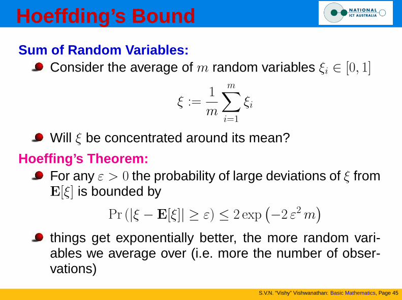
Hoeffding’s Bound
S.V.N. “Vishy” Vishwanathan: Basic Mathematics, Page 45
Sum of Random Variables:Consider the average of m random variables ξi ∈ [0, 1]
ξ :=1
m
m∑i=1
ξi
Will ξ be concentrated around its mean?
Hoeffing’s Theorem:For any ε > 0 the probability of large deviations of ξ fromE[ξ] is bounded by
Pr (|ξ − E[ξ]| ≥ ε) ≤ 2 exp(−2 ε2 m
)things get exponentially better, the more random vari-ables we average over (i.e. more the number of obser-vations)
Page 46
Questions?
S.V.N. “Vishy” Vishwanathan: Basic Mathematics, Page 46