Basic properties of the infinite critical-FK random map

Linxiao Chen

To cite this version:

Linxiao Chen. Basic properties of the infinite critical-FK random map. 16 pages, 6 figures.2015. <hal-01120810>

HAL Id: hal-01120810

https://hal.archives-ouvertes.fr/hal-01120810

Submitted on 3 Mar 2015

HAL is a multi-disciplinary open accessarchive for the deposit and dissemination of sci-entific research documents, whether they are pub-lished or not. The documents may come fromteaching and research institutions in France orabroad, or from public or private research centers.

L’archive ouverte pluridisciplinaire HAL, estdestinee au depot et a la diffusion de documentsscientifiques de niveau recherche, publies ou non,emanant des etablissements d’enseignement et derecherche francais ou etrangers, des laboratoirespublics ou prives.

Basic properties of the infinite critical-FK random map

Linxiao Chen∗

Abstract

We consider the critical Fortuin-Kasteleyn (cFK) random map model. For each q ∈ [0,∞]and integer n ≥ 1, this model chooses a planar map of n edges with probability proportionalto the partition function of critical q-Potts model on that map. Sheffield introduced thehamburger-cheeseburger bijection which sends the cFK random maps to a family of randomwords, and remarked that one can construct infinite cFK random maps using this bijection.We make this idea precise by a detailed proof of the local convergence using a monotonicityresult which compares the model with general value of q to the case q = 0. When q = 1,this provides an alternative construction of the UIPQ. In addition, we show that for any q,the limit is almost surely one-ended and recurrent for the simple random walk.

1 IntroductionPlanar maps. Random planar maps has been the focus of intensive research in recentyears. We refer to [1] for the physics background and motivations, and to [23] for a surveyof recent results in the field.

A finite planar map is a proper embedding of a finite connected graph into the two-dimensional sphere, viewed up to orientation-preserving homeomorphisms. Self-loops andmultiple edges are allowed in the graph. In this paper we will not deal with non-planar maps,and thus we drop the adjective “planar” sometimes. The faces of a map are the connectedcomponents of the complement of the embedding in the sphere and the degree of a face isthe number of edges incident to it. A map is a triangulation (resp. a quadrangulation) if allof its faces are of degree three (resp. four). The dual map M† of a planar map M has onevertex associated to each face of M and there is an edge between two vertices if and only iftheir corresponding faces in M are adjacent.

A corner in a planar map is the angular section delimited by two consecutive half-edgesaround a vertex. It can be identified with an oriented edge using the orientation of thesphere. A rooted map is a map with a distinguished oriented edge or, equivalently, a corner.We call root edge the distinguished oriented edge, and root vertex (resp. root face) the vertex(resp. face) incident to the distinguished corner. Rooting a map on a corner (instead of themore traditional choice of rooting on an oriented edge) allows a canonical choice of the rootfor the dual map: the dual root is obtained by exchanging the root face and the root vertex.A subgraph of a planar map is a graph consisting of a subset of its edges and all of its vertices.Given a subgraph G of a map M, the dual subgraph of G, denoted by G†, is the subgraphof M† consisting of all the edges that do not intersect G. Following the terminology in [5],we call subgraph-rooted map a rooted planar map with a distinguished subgraph. Fig. 1(a)gives an example of a subgraph-rooted map with its dual map.

Local limit. For subgraph-rooted maps, the local distance is defined by

dloc((M,G), (M′,G′)) = inf{

2−R∣∣R ∈ N, BR(M,G) = BR(M′,G′)

}(1)

where BR(M,G), the ball of radius R in (M,G), is the subgraph-rooted map consisting ofall vertices of M at graph distance at most R from the root vertex and the edges betweenthem. An edge of BR(M,G) belongs to the distinguished subgraph of BR(M,G) if andonly if it is in G. The space of all finite subgraph-rooted maps is not complete with respectto dloc and we denote by M its Cauchy completion. We call infinite subgraph-rooted map

∗ Institut de Physique Théorique, CEA/DSM/IPhT – CNRS UMR 3681, F-91191 Gif sur Yvette Cedex andUniversité Paris-Sud. E-mail: linxiao.chen@math.u-psud.fr

1

arX

iv:1

502.

0101

3v1

[m

ath.

PR]

3 F

eb 2

015

(M,G) (M†,G†) (G |G†)

(a) (b)

Figure 1: (a) A subgraph-rooted map and its dual. Edges of the distinguished subgraph aredrawn in solid line, and the other edges in dashed line. The root corner is indicated by an arrow.(b) Loops separating the distinguished subgraph and its dual subgraph.

the elements ofM which are not finite subgraph-rooted map. Note that with this definitionall infinite maps are locally finite, that is, every vertex is of finite degree.

The study of infinite random maps goes back to the works of Angel, Benjamini andSchramm on the Uniform Infinite Planar Triangulation (UIPT) [3, 2] obtained as the locallimit of uniform triangulations of size tending to infinity. Since then variants of this theoremhave been proved for different classes of maps [12, 21, 22, 13, 7]. A common point of thethese infinite random lattices is that they are constructed from the uniform distribution onsome finite sets of planar maps. In this work, we consider a different type of distribution.

cFK random map. For n ≥ 1 we write Mn for the set of all subgraph-rooted mapswith n edges. Recall that in a dual subgraph-rooted maps, the distinguished subgraph Gand its dual subgraph G† do not intersect. Therefore we can draw a set of loops tracing theboundary between them, as in Fig. 1(b). Let `(M,G) be the number of loops separating G

and G†. For each q > 0, let Q(q)n be the probability distribution onMn defined by

Q(q)n (M,G) ∝ q

12 `(M,G) (2)

By taking appropriate limits, we can define Q(q)n for q ∈ {0,∞}. A critical Fortuin-Kasteleyn

(cFK) random map of size n and of parameter q is a random variable of law Q(q)n (see

Equation (5) below for the connection with the Fortuin-Kasteleyn random cluster model).From the definition of the loop number `, it is easily seen that the law Q(q)

n is self-dual(which is why we call it critical):

Q(q)n (M,G) = Q(q)

n (M†,G†) (3)

Our main result is:

Theorem 1. For each q ∈ [0,∞], we have Q(q)n −−−−→

n→∞Q(q)∞ in distribution with respect to

the metric dloc, where Q(q)∞ is a probability distribution on infinite subgraph-rooted maps.

Moreover, if (M,G) has law Q(q)∞ , then

• we have (M,G) = (M†,G†) in distribution,

• the map M is almost surely one-ended and recurrent for the simple random walk.

So far two main methods have been developed to prove local convergence of finite randommaps. The first one, initially used in [2] is based on precise asymptotic enumeration formulasfor certain classes of maps. Although enumeration results about (a generalization of) cFKdecorated maps have been obtained using combinatorial techniques [20, 15, 6, 17, 10, 9, 8],we are not going to follow this approach here. We will rather first transform our finite mapmodel through a bijection into simpler objects. The archetype of such bijection is the famousCori-Vauqulin-Schaeffer bijection and its generalizations [24, 11]. Then we take local limitsof these simpler objects and construct the limit of the maps directly from the latter. Thistechnique has been used e.g. in [12, 13, 7]. In this work the role of the Schaeffer bijection will

2

be played by Sheffield’s hamburger-cheeseburger bijection [25] which maps a cFK randommap to a random word in a measure-preserving way. We will then construct the local limitof cFK random maps by showing that the random word converges locally to a limit, andthat the hamburger-cheeseburger bijection has an almost surely continuous extension forthat limit.

Let us mention two related works [19, 4] which were posted by independent teams onarXiv just before this work. [19] studied fine properties of the scaling limit of the infinitecFK random map in a topology defined via the hamburger-cheeseburger bijection. Both[19] and [4] derived the critical exponents associated to the length and the enclosed areaof a loop in the infinite cFK random map, referring to [25] for its existence. The proposeof this work is to give a detailed proof of the local convergence of finite cFK random mapsto its infinite-volume limit (and establish its recurrence). Our methods rely principally onconstructions of bijections and classical results on simple random walks.

The rest of this paper is organized as follows. In Section 2 we discuss in more detailsthe law of the cFK random map and discuss interesting special cases. In Section 3 we firstdefine the random word model underlying the hamburger-cheeseburger bijection. Then weshow that the model has an explicit local limit, and proves some properties of the limit.In Section 4 we construct the hamburger-cheeseburger bijection and proves Theorem 1 bytranslating the properties of the infinite random word in terms of the maps.

Acknowledgements. This work comes essentially from my master thesis. I thankdeeply my advisors Jérémie Bouttier and Nicolas Curien. I thank also the Isaac Newton In-stitute and the organizers of the Random Geometry programme for their hospitality duringthe completion of this work. This work is supported in part by ANR project “Cartaplus”12-JS02-001-01.

2 More on cFK random mapLet (M,G) be a subgraph-rooted map and denote by c(G) the number of connected compo-nents in G. Recalling the definition of `(M,G) given in the introduction, it is not difficultto see that `(M,G) = c(G) + c(G†)− 1. However c(G†) is nothing but the number of facesof G, therefore by Euler’s relation we have

`(M,G) = e(G) + 2c(G)− v(M), (4)

where e(G) is the number of edges G, and v(M) is the number of vertices in M. This givesthe following expression of the first marginal of Q(q)

n : for all rooted map M with n edges,we have

Q(q)n (M) ∝ q− 1

2v(M)∑

G⊂M

√qe(G)

qc(G). (5)

The sum on the right-hand side over all the subgraphs of M is precisely the partition functionof the Fortuin-Kasteleyn random cluster model or, equivalenty, of the Potts model on themap M (The two partition functions are equal. See e.g. [16, Section 1.4]. See also [8, Section2.1] for a review of their connection with loop models on planar lattices). For this reason,the cFK random map is used as a model of quantum gravity theory in which the geometry ofthe space interacts with the matter (spins in the Potts model). Note that the “temperature”in the Potts model and the prefactor q−

12 v(M) in (5) are tuned to ensure self-duality, which

is crucial for our result to hold.Three values of the parameter q deserve special attention, since the cFK random map

has nice combinatorial interpretations in these cases.

q = 0: Q(0)n is the uniform measure on the elements of Mn which minimize the number

of loops `. The minimum is `min = 1 and it is achieved if and only if the subgraph G

is a spanning tree of M. Therefore under Q(0)n , the map M is chosen with probability

proportional to the number of its spanning trees, and conditionally on M, G is a uniformspanning tree of M.

At the limit, the marginal law of G under Q(0)∞ will be that of a critical geometric

Galton-Walton tree conditioned to survive. This will be clear once we defined the hamburger-cheeseburger bijection. In fact when q = 0, the hamburger-cheeseburger bijection is reducedto a bijection between tree-rooted maps and excursions of simple random walk on Z2 intro-duced earlier by Bernardi [5].

3

q = 1: Q(1)n is the uniform measure onMn. Since each planar map with n edges has 2n

subgraphs, M is a uniform planar map chosen among the maps with n edges. Thus in thecase q = 1, Theorem 1 can be seen as a construction of the Uniform Infinite Planar Mapor of the Uniform Infinite Planar Quadrangulation via Tutte’s bijection. It is a curious factthat with this approach, one has to first decorate a uniform planar map with a randomsubgraph in order to show the local convergence of the map. As we will see later, the couple(M,G) is encoded by the hamburger-cheeseburger bijection in a entangled way.

q =∞: Similarly to the case q = 0, the probability Q(∞)n is the uniform measure on

the elements of Mn which maximize `. To see what are these elements, remark that eachconnected component of G contains at least one vertex, therefore

c(G) ≤ v(M) (6)

And, at least one edge must be removed from M to create a new connected component, so

c(G) ≤ c(M) + e(M)− e(G) = n+ 1− e(G) (7)

Summing the two relations, we see that the maximal number of loops is `max = n+ 1 and itis achieved if and only if each connected component of G contains exactly one vertex (i.e. alledges of G are self-loops) and that the complementary subgraph M\G is a tree. Fig. 2(a)gives an example of such couple (M,G).

(a) (b)

Figure 2: (a) A subgraph-rooted map which maximizes the number of loops `. Colors are usedonly to illutrate the bijection. (b) The percolation configuration on a rooted tree associated tothis map by the bijection. The divided vertices, as well as the replaced edges, are drawn in thesame color before and after the bijection.

This model of loop-decorated tree is in bijection with bond percolation of parameter 1/2on a uniform random plane tree with n edges, as we now explain. For a couple (M,G)satisfying the above conditions, consider a self-loop e in G. This self-loop separates the restof the map M into two parts which share only the vertex of e. We divide this vertex intwo, and replace the self-loop e by an edge joining the two child vertices. The new edge isalways considered part of G. By repeating this operation for all self-loops in the subgraphG in an arbitrary order, we transform the map M into a rooted plane tree, see Fig. 2.This gives a bijection from the support of Q(∞)

n to the set of rooted plane tree of n edgeswith a distinguished subgraph. The latter object converges locally to a critical geometricGalton-Watson tree conditioned to survive, in which each edge belongs to the distinguishedsubgraph with probability 1/2 independently from other edges. Using the inverse of thebijection above (which is almost surely continuous at the limit), we can explicit the lawQ(∞)∞ . In particular, it is easily seen that M is almost surely a one-ended tree plus finitely

many self-loops at each vertex. Therefore it is one-ended and recurrent.

3 Local limit of random wordsIn this section we define the random word model underlying the hamburger-cheeseburgerbijection, and establish its local limit.

4

We consider words on the alphabet Θ = {a, b, A, B, F}. Formally, a word w is a mappingfrom an interval I of integers to Θ. We write w ∈ ΘI and we call I the domain of w. LetW be the space of all words, that is,

W =⋃I

ΘI (8)

where I runs over all subintervals of Z. Note that a word can be finite, semi-infinite or bi-infinite. We denote by ∅ the empty word. Given a word w of domain I and k ∈ I, we denoteby wk the letter of index k in w. More generally, if J is an (integer or real) interval, we denoteby wJ the restriction of the word w to I ∩ J . For example, if w = bAbaFABa ∈ Θ{0,...,7},then w[2,6) = baFA ∈ Θ{2,3,4,5}. We endow W with the local distance

Dloc(w,w′) = inf

{2−R

∣∣∣R ∈ N, w[−R,R) = w′[−R,R)

}(9)

Note that the equality w[−R,R) = w′[−R,R) implies that I ∩ [−R,R) = I ′ ∩ [−R,R), whereI (resp. I ′) is the domain of the word w (resp. w′). It is easily seen that (W, Dloc) is acompact metric space.

3.1 Reduction of wordsNow we define the reduction operation on the words. For each word w, this operationspecifies a pairing between letters in the word called matching, and returns two shorterwords wλ and wΛ.

We follow the exposition given in [25]. The letters a, b, A, B, F are interpreted as, respec-tively, a hamburger, a cheeseburger, a hamburger order, a cheeseburger order and a flexibleorder. They obey the following order fulfillment relation: a hamburger order A can only befulfilled by a hamburger a, a cheeseburger order B by a cheeseburger b, while a flexible orderF can be fulfilled either by a hamburger a or by a cheeseburger b. We write λ = {a, b} andΛ = {A, B, F} for the set of lowercase letters (burgers) and uppercase letters (orders).

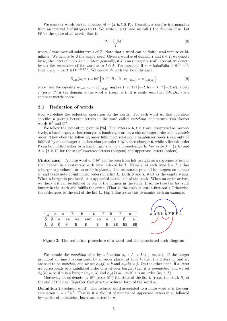
Finite case. A finite word w ∈ ΘI can be seen from left to right as a sequence of eventsthat happen in a restaurant with time indexed by I. Namely, at each time k ∈ I, eithera burger is produced, or an order is placed. The restaurant puts all its burgers on a stackS, and takes note of unfulfilled orders in a list L. Both S and L start as the empty string.When a burger is produced, it is appended at the end of the stack. When an order arrives,we check if it can be fulfilled by one of the burgers in the stack. If so, we take the last suchburger in the stack and fulfills the order. (That is, the stack is last-in-first-out.) Otherwise,the order goes to the end of the list L. Fig. 3 illustrates this dynamics with an example.

wk a a B b A F B F a

S ∅ a aa aa aab ab a a ∅ a

L ∅ ∅ ∅ B B B B BB BB BB

a Fa b BAB aF

Figure 3: The reduction procedure of a word and the associated arch diagram

We encode the matching of w by a function φw : I → I ∪ {−∞,∞}. If the burgerproduced at time j is consumed by an order placed at time k, then the letters wj and wkare said to be matched, and we set φw(j) = k and φw(k) = j. On the other hand, if a letterwk corresponds to a unfulfilled order or a leftover burger, then it is unmatched, and we setφw(k) =∞ if it is a burger (wk ∈ λ) and φw(k) = −∞ if it is an order (wk ∈ Λ).

Moreover, let us denote by wΛ (resp. wλ) the state of the list L (resp. the stack S) atthe end of the day. Together they give the reduced form of the word w.

Definition 2 (reduced word). The reduced word associated to a finite word w is the con-catenation w = wΛwλ. That is, it is the list of unmatched uppercase letters in w, followedby the list of unmatched lowercase letters in w.

5

The matching and the reduced word can be represented as an arch diagram as follows.For each letter wj in the word w, draw a vertex in the complex plane at position j. For eachpair of matched letters wj and wk, draw a semi-circular arch that links the correspondingpair of vertices. This arch is drawn in the upper half plane if it is incident to an a-vertex,and in the lower half plane if it is incident to a b-vertex. For an unmatched letter wj , wedraw an open arch from j tending to the left if φw(j) = −∞, or to the right if φw(j) =∞.See Fig. 3.

It should be clear from the definition of matching operation that the arches in thisdiagram do not intersect each other. We shall come back to this diagram in Section 4 toconstruct the hamburger-cheeseburger bijection.

Infinite case. Remark that a hamburger produced at time j is consumed by a hamburgerorder at time k > j if and only if 1) all the hamburgers produced during the interval[j+ 1, k− 1] are consumed strictly before time k, and 2) all the hamburger or flexible ordersplaced during [j + 1, k− 1] are fulfilled by a burger produced strictly after time j. In termsof the reduced word, this means that two letters wj = a and wk = A are matched if and onlyif w(j,k) does not contain any a, A or F. This can be generalized to any pair of burger/order.

Proposition 3 ([25]). For j < k, assume that wj ∈ λ and wk ∈ Λ can be matched. Thenthey are matched in w if and only if w(j,k) does not contain any letter that can be matchedto either wj or wk.

This shows that the matching rule is entirely determined by the reduction operator. Moreimportantly, we see that the matching rule is local, that is, whether φw(j) = k or not onlydepends on w[j,k]. From this we deduce that the reduction operator is compatible with stringconcatenation, that is, uv = uv = uv for any pair of finite words u, v.

This locality property allows us to define φw for infinite words w. Then, we can also readwλ (resp. wΛ) from φw as the (possibly infinite) sequence of unmatched lowercase (resp.uppercase) letters. However w is not defined in general, since the concatenation wΛwλ doesnot always make sense.

Random word model and local limit. For each p ∈ [0, 1], let θ(p) be the probabilitymeasure on Θ such that

θ(p)(a) = θ(p)(b) =1

4θ(p)(A) = θ(p)(B) =

1− p4

θ(p)(F) =p

2

Here p should be interpreted as the proportion of flexible orders among all the orders.Remark that, regardless of the value of p, the distribution is symmetric when exchanging a

with b and A with B. As we will see in Section 4, this corresponds to the self-duality of cFKrandom maps.

For n ≥ 1, let Ik = {−k, . . . , 2n− 1− k}, and set

Wn =⋃

0≤k<2n

{w ∈ ΘIk

∣∣w = ∅}

(10)

For p ∈ [0, 1], let P(p)n be the probability measure on Wn proportional to the direct product

of θ(p), that is, for all w ∈ Wn,

P(p)n (w) ∝

∏j

θ(p)(wj) (11)

where the product is taken over the domain of w. In addition, let P(p)∞ = θ(p)⊗Z be the

product measure on bi-infinite words. Our proof of Theorem 1 relays mainly on the followingproposition, stated by Sheffield in an informal way in [25].

Proposition 4. For all p ∈ [0, 1], we have P(p)n → P(p)

∞ in law for Dloc as n→∞.

3.2 Proof of Proposition 4We follow the approach proposed by Sheffield in [25, Section 4.2]. Let W (p) be a randomword of law P(p)

∞ , so that W (p)[0,n) is a word of length n with i.i.d. letters. As a step in the

proof, we will need to show that the extinction probability

P(W

(p)[0,2n) = ∅

)(12)

6

decays sub-exponentially as n→∞. This could be proved using the result of [25], howeverwe present here a direct proof, which leads to a slightly more precise estimate and is basedon the following stochastic inequality.

Lemma 5. For any p ∈ [0, 1] and n ∈ N, the word W(p)[0,n) is stochastically shorter than

W(0)[0,n). That is, for any c ≥ 0,

P(∣∣∣W (p)

[0,n)

∣∣∣ ≥ c) ≤ P(∣∣∣W (0)

[0,n)

∣∣∣ ≥ c) (13)

This result is intuitive, because p is the proportion of flexible orders, and the presence offlexible orders should makes order fulfillment easier, leaving less burgers or unfulfilled ordersat the end. We postpone the proof of this lemma to Appendix A. Here let us deduce anestimate of the extinction probability (12) from it.

When p = 0, the flexible order F never appears. For k ≥ 0, let Xk the net count ofhamburgers at time k, that is, Xk = (#a)W[0,k) − (#A)W[0,k). Define Yk similarly forcheeseburgers. Then (Xk, Yk)k≥0 is a simple random walk on Z2 starting from the origin.And the extinction probability

P(W

(0)[0,2n) = ∅

)(14)

is the probability that this simple random walk makes an excursion of 2n-steps in the firstquadrant {(x, y) : x ≥ 0, y ≥ 0}. It is well known [5] that the number of such excursionsis Catn·Catn+1, where Catn = 1

n+1

(2nn

)is the n-th Catalan number. Using the preceding

lemma, we obtain the following estimate: for any p ∈ [0, 1],

P(W

(p)[0,2n) = ∅

)≥ 1

42nCatn·Catn+1 =

4

π

1

n3(1 + o(1)) (15)

Proof of Proposition 4. By compactness of (W, Dloc), it suffices to show that for any ballBloc in this space, we have P(p)

n (Bloc)−→P(p)∞ (Bloc). Note that Dloc is an ultrametric and

the ball Bloc(w, 2−R) of radius 2−R around w is the set of words which are identical to w

when restricted to [−R,R). In the rest of the proof, we fix an integer R ≥ 1 and a wordw ∈ Θ[−R,R)∩Z. Recall that W (p) has law P(p)

∞ . In the following we omit the parameter pfrom the superscripts to keep simple notations.

Recall that the space Wn is made up of 2n copies of the set{w ∈ Θ2n

∣∣w = ∅}differing

from each other by translation of the indices. Therefore Pn can be seen as the conditionallaw of W[−K,2n−K) on the event {W[−K,2n−K) = ∅}, where K is a uniform random variableon {0, . . . , 2n− 1} independent from W . Moreover, for the word W[−K,2n−K) to have w asits restriction to [−R,R), one must to have R ≤ K ≤ 2n−R. Hence,

Pn(Bloc(w, 2

−R))

= P(R ≤ K ≤ 2n−R and W[−R,R) = w

∣∣W[−K,2n−K) = ∅)

=1

2n

2n−R∑k=R

P(W[−R,R) = w

∣∣W[−k,2n−k) = ∅)

=1

2n

2n−2R∑k=0

P(W[k,k+2R) ' w

∣∣W[0,2n) = ∅)

= E

[1

2n

2n−2R∑k=0

1{W[k,k+2R)'w}

∣∣∣∣∣W[0,2n) = ∅]

where in the last two steps, we denote by u ' v the fact that two words are equal up to anoverall translation of indices. On the other hand, set

πw = P(Bloc(w, 2−R)) =

R−1∏k=−R

θ(wk) (16)

By translation invariance of W we have

E

[1

2n

2n−2R∑k=0

1{W[k,k+2R)'w}

]=

2n− 2R+ 1

2nπw (17)

7

In fact, up to boundary terms of the order O(R/n), the quantity inside the expectation isthe empirical measure of the Markov chain (W[k,k+2R))k≥0 taken at the state w. This isan irreducible Markov chain on the finite state space Θ2R. Sanov’s theorem (see e.g. [14,Theorem 3.1.2]) gives the following large deviation estimate. For any ε > 0, there areconstants Aε, Cε > 0 depending only on ε and on the transition matrix of (W[k,k+2R))k≥0,such that

P

(∣∣∣ 1

2n

2n−2R∑k=0

1{W[k,k+2R)'w} − πw∣∣∣ > ε

)≤ Aεe−Cεn (18)

for all n ≥ 1. Since∣∣∣∣ 1

2n

2n−2R∑k=0

1{W[k,k+2R)'w} − πw∣∣∣∣ is bounded by 1, we have

∣∣Pn (Bloc(w, 2−R)

)− πw

∣∣ ≤ E

[∣∣∣ 1

2n

2n−2R∑k=0

1{W[k,k+2R)'w} − πw∣∣∣ ∣∣∣∣∣W[0,2n) = ∅

]

≤ ε+ P

(∣∣∣ 1

2n

2n−2R∑k=0

1{W[k,k+2R)'w} − πw∣∣∣ > ε

∣∣∣∣∣W[0,2n) = ∅)

≤ ε+1

P(W[0,2n) = ∅

) · P(∣∣∣ 1

2n

2n−2R∑k=0

1{W[k,k+2R)'w} − πw∣∣∣ > ε

)

≤ ε+Aεe

−Cεn

P(W[0,2n) = ∅

)By (15) the second term converges to zero as n→∞. Since ε can be taken arbitrarily closeto zero, this shows that Pn

(Bloc(w, 2

−R))→ πw as n→∞.

3.3 Some properties of the limiting random wordIn this section we show two properties of the infinite random word W (p) which will be theword-counterpart of Theorem 1. Both properties are true for general p ∈ [0, 1]. However wewill only write proofs for p < 1, since the case p = 1 corresponds to cFK random maps withparameter q = ∞, for which the local limit is explicit. (The proofs for p = 1 are actuallyeasier, but they require different arguments.)

Proposition 6 (Sheffield [25]). For all p ∈ [0, 1], almost surely,

1. W (p) = ∅, that is, every letter in W (p) is matched.

2. For all k ∈ Z, W (p)(−∞,k)

λ

contains infinitely many a and infinitely many b.

Proof. The first assertion is proved as Proposition 2.2 in [25]. For the second assertion,

recall that W (p)(−∞,k)

λ

represents a left-infinite stack of burgers. Now assume for some k ∈ Z,

it contains only N letters a with positive probability. Then, with probability(

1−p4

)N+1and

independently of W (p)(−∞,k), all the N + 1 letters in W (p)

[k,k+N ] are A. This will leave the A atposition k+N unmatched in W , which happens with zero probability according to the firstassertion. This gives a contradiction when p < 1.

For each random word W (p), consider a random walk Z on Z2 starting from the origin:Z0 = (0, 0), and for all k ∈ Z,

Zk+1 − Zk =

(1, 0) if W (p)

k = a

(−1, 0) if W (p)k is matched to an a

(0, 1) if W (p)k = b

(0,−1) if W (p)k is matched to a b

(19)

By Proposition 6, Zk is almost surely well-defined for all k ∈ Z. A lot of information aboutthe random word W can be read from Z. The main result of [25] shows that under diffusiverescaling, Z converges to a Brownian motion in R2 with a diffusivity matrix that dependson p, demonstrating a phase transition at p = 1/2.

8

Let (X,Y ) = Z. Set i0 = sup {i < 0 |Xi = −1} and j0 = inf {j > 0 |Xj = −1}. Let N0

be the number of times that X visits the state 0 between time i0 and j0. We shall see inSection 4.2 that N0 is exactly the degree of root vertex in the infinite cFK-random map.Below we prove that the distribution of N0 has an exponential tail, that is, there existsconstants A and c > 0 such that P(N0 ≥ x) ≤ Ae−cx for all x ≥ 0.

...... ......

......S0=0 T0 S1 T1 SK

TK=j0

SK+1 TK+1 SM

TM

a a a

F A

......

Xt

Figure 4: The decomposition of N+0 into intervals [Sk, Tk]

.

Proposition 7. N0 has an exponential tail distribution for all p ∈ [0, 1].

Proof. First let us consider N+0 , the number of times that X visits the state 0 between time

0 and j0. Remark that at positive time, the process X is adapted to the natural filtration(Fk)k≥0, where Fk is the σ-algebra generated byW[0,k). Define two sequences of F-stoppingtimes (Sm)m≥0 and (Tm)m≥0 by S0 = 0, and that for all m ≥ 0,

Tm = inf {k > Sm |Xk 6= 0}Sm+1 = inf {k > Tm |Xk = 0}

The sequence S (resp. T ) marks the times that X arrives at (resp. departs from) the state 0.Therefore the total number of visits of the state 0 between time 0 and Tm is

∑mi=0(Ti−Si),

see Fig. 4.By construction, j0 is the smallest Tm such that XTm = −1. On the other hand, we have

XTm∈ {−1,+1} for all m and

XTm = +1 ⇔ WTm = a

XTm = −1 ⇔ WTm = A or WTm is an F matched to an a

Consider the stopping time

M = inf {m ≥ 0 |WTm = A} (20)

Then we have j0 ≤ TM , and therefore

N+0 ≤

M∑m=0

(Tm − Sm) (21)

On the other hand,M is the smallest m such that, starting from time Sm, an A comes beforean a. Therefore M is a geometric random variable of mean 1−p

p .Assume p < 1 so that M is almost surely finite. Fix an integer m ≥ 0. By the strong

Markov property, conditionally to {M = m}, the sequence (Ti − Si, i = 0 . . .m − 1) isi.i.d., and each term in the sequence has the same law as the first arrival time of a in thesequence (Wk)k≥0 conditioned not to contain A. In other words, conditionally to {M = m},(Ti − Si, i = 0 . . .m − 1) is an i.i.d. sequence of geometric random variables of mean 1

2+p .Similarly, conditionally to {M = m}, Tm − Sm is a geometric random variable of mean 1−p

2+p

independent from the sequence (Ti − Si, i = 0 . . .m− 1). Then, a direct computation showsthat the exponential moment E[eλN

+0 ] is finite for some γ > 0. And by Markov’s inequality,

the distribution of N+0 has an exponential tail when p < 1.

Now we claim that conditionally to the value of N0, the variable N+0 is uniform on

{1, . . . , N0} which implies that N0 also has an exponential tail distribution. To see whythe conditional law is uniform, consider N0 and N+

0 for finite words defined in the sameway as for the infinite word W

(p)∞ . Note that for a finite word w the process X does not

9

necessarily hit −1 at negative (resp. positive) times. In this case we just replace i0 (resp.j0) by the infimum (resp. supremum) of the domain of w. Then, w 7→ (N0, N

+0 ) is a Dloc-

continuous function defined on the union of ∪n≥0Wn and the support of W (p)∞ . Therefore

for any integers k ≤ m,

P(p)n (N0 = m,N+

0 = k) −−−−→n→∞

P(p)∞ (N0 = m,N+

0 = k) (22)

But, given the sequence of letters in a word, the law P(p)n chooses the letter of index 0

uniformly at random among all the letters. A simple counting shows that for all 1≤k, k′≤m,we have P(p)

n (N0 = m,N+0 = k) = P(p)

n (N0 = m,N+0 = k′). Letting n → ∞ shows that the

conditional law of N+0 given N0 is uniform under P(p)

∞ .

4 The hamburger-cheeseburger bijection

4.1 ConstructionIn this section we present (a slight variant of) the hamburger-cheeseburger bijection ofSheffield. We refer to [25] for the proof of bijectivity and for historical notes.

We define the hamburger-cheeseburger bijection Ψ on a subset of the space W, and ittakes values in the space M of doubly-rooted planar maps with a distinguished subgraph,that is, planar maps with two distinguished corners and one distinguished subgraph. Wecan write this space as

M = {(M,G, s) | (M,G) ∈M and s is a corner of M} (23)

Note that the second root s may be equal to or different from the root of M. We define inthe same way Mn, the doubly-rooted version of the spaceMn. Its cardinal is 2n times thatofMn.

We start by constructing Ψ :Wn → Mn in three steps. The first step transforms a wordin Wn into a decorated planar map called arch graph. The second and the third step applygraph duality and local transformations to the arch graph to get a tree-rooted map, and thena subgraph-rooted map in Mn.

Step 1: from words to arch graphs. Fix a word w ∈ Wn. Recall from Section3 the construction of the non-crossing arch diagram associated to w. In particular sincew = ∅, there is no half-arch. We link neighboring vertices by unit segments [j − 1, j] andlink the first vertex to the last vertex by an edge that wires around the whole picture withoutintersecting any other edges. This defines a planar map A of 2n vertices and 2n edges. InA we distinguish edges coming from arches and the other edges. The latter forms a simpleloop passing through all the vertices.

We further decorate A with additional pieces of information. Recall that the word wis indexed by an interval of the form Ik = {−k, . . . , 2n − 1 − k} where 0 ≤ k < 2n. Wewill mark the oriented edge r from the vertex 0 to the vertex −1, and the oriented edge sfrom the first vertex (−k) to the last vertex (2n − 1 − k). If k = 0, then r and s coincide.Furthermore, we mark each arch incident to an F-vertex by a star ∗. (See Fig. 5) We call thedecorated planar map A the arch graph of w. One can check that it completely determinesthe underlying word w.

Step 2: from arch graphs to tree-rooted maps. We now consider the dual map∆ of the arch graph A. Let Q be the subgraph of ∆ consisting of edges whose dual edge ison the loop in A. We denote by ∆\Q the set of remaining edges of ∆ (that is, the edgesintersecting one of the arches).

Proposition 8. The map ∆ is a triangulation, the map Q is a quadrangulation with nfaces and ∆\Q consists of two trees.

We denote by T and T† the two trees in ∆\Q, with T corresponding to faces of thearch graph in the upper half plane. Then Q, T and T† form a partition of edges in thetriangulation ∆. Note that T and T† give the (unique) bipartition of vertices of Q. Let Mbe the planar map associated to Q by Tutte’s bijection, such that M has the same vertexset as T. (The latter prescription allows us to bypass the root, and define Tutte’s bijection

10

from unrooted quadrangulations to unrooted maps.) We thus obtain a couple (M,T) inwhich M is a map with n edges and T is spanning tree of M. Remark that T† is the dualspanning tree of T in the dual map M†. This relates the duality of maps with the dualityon words which consists of exchanging a with b and A with B.

Fig. 5(a) summarizes the mapping from words to tree-rooted maps (Step 1 and 2) withan example. Note that we have omitted the two roots and the stars on the arch graph in theabove discussion. But since graph duality and Tutte’s bijection provide canonical bijectionsbetween edges, the roots and stars can be simply transferred from the arches in A to theedges in M. With the roots and stars taken into account, it is clear that w 7→ (M,T) is abijection from Wn onto its image.

∗∗

∗

∗

∗

∗

∗

∗

∗

ab Faa b ABAB Fab Fw =

A ∆ = Q ∪T ∪T† (M,T)arch graph dual map Tutte’s bijection

Q→Mw

(a)

1-2 50-1 3 9642 108-3 7

(M,T) (M,G)

∗

∗

∗

∗

∗

∗

switch starred edges(b)

Figure 5: Construction of the hamburger-cheeseburger bijection. (a) From word to tree-rootedmap. (b) From tree-rooted map to subgraph-rooted map.

Step 3: from tree-rooted maps to subgraph-rooted maps. Now we “switchthe status” of every starred edge in M relative to the spanning tree T. That is, if a starrededge is not in T, we add it to T; if it is already in T, we remove it from T. Let G be theresulting subgraph. See Fig. 5(b) for an example.

Recall that there are two marked corners r and s in the map M. By an abuse of notation,from now on we denote by M the rooted map with root corner r. Then, the hamburger-cheeseburger bijection is defined by Ψ(w) = (M,G, s). Let Ψ(w) = (M,G) be its projectionobtained by forgetting the second root corner. We denote by (#F)w the number of lettersF in w, and by ` the number of loops associated to the corresponding subgraph-rooted map(M,G).

Theorem 9 (Sheffield [25]). The mapping Ψ : Wn → Mn is a bijection such that ` =

1 + (#F)w for all w ∈ Wn. And Q(q)n is the image measure of P(p)

n by Ψ whenever

p =

√q

2 +√q.

Proof. The proof of this can be found in [25]. However we include a proof of the second factto enlighten the relation p =

√p

2+√q . For w ∈ Wn, since w = ∅, we have (#a)w + (#b)w =

11

(#A)w + (#B)w + (#F)w = n. Therefore, when p =√q

2+√q ,

P(p)n (w) ∝

(1

4

)(#a)w+(#b)w (1− p

4

)(#A)w+(#B)w (p2

)(#F)w

=

(1

4

)n(1− p

4

)n−(#F)w (p2

)(#F)w

∝(

2p

1− p

)(#F)w

=√q`−1

After normalization, this shows that Q(q)n is the image measure of P(p)

n by Ψ.

Proposition 10. We can extend the mapping Ψ to W →M so that it is P(p)∞ -almost surely

continuous with respect to Dloc and dloc, for all p ∈ [0, 1].

Proof. Observe that if we do not care about the location of the second root s, then the wordw used in the construction of Ψ does not have to be finite. Set

W∞ =

{w ∈ ΘZ

∣∣∣∣ w = ∅ and for all k ∈ Z, w(−∞,k)λ contains

infinitely many a and infinitely many b

}(24)

We claim that indeed, for each w ∈ W∞, Step 1, 2 and 3 of the construction define a (locallyfinite) infinite subgraph-rooted map: as in the case of finite words, the condition w = ∅ensures that the arch graph A of w is a well-defined infinite planar map (that is, all thearches are closed). To see that its dual map ∆ is a locally finite, infinite triangulation,we only need to check that each face of A has finite degree. Observe that a letter a in wappears in w(−∞,k)

λ if and only if it is on the left of wk, and that its partner is on the rightof wk. This corresponds to an arch passing above the vertex k. Therefore, the remainingcondition in the definition of W∞ says that there are infinitely many arches which passabove and below each vertex of A. This guarantees that A has no unbounded face. Therest of the construction consists of local operations only. So the resulting subgraph-rootedmap (M,G) = Ψ(w) is a locally finite subgraph-rooted map.

Also, by Proposition 6, we have P(p)∞ (W∞) = 1. It remains to see that (the extension)

of Ψ is continuous on W ′ =⋃nWn ∪W∞. Let w(n), w ∈ W ′ so that w(n) → w for Dloc. If

w is finite, there is nothing to prove. Otherwise, let (M,G) = Ψ(w) and consider a ball Bof finite radius r around the root in the map M. By locality of the mapping ∆ M, theball B can be determined by a ball B′ of finite radius r′ (which may depend on M) in ∆.But each triangle in ∆ corresponds to a letter in the word, so there exists r′′ (which maydepend on M) such that if w(n)

[−r′′,r′′] = w[−r′′,r′′] then the balls of radius r′ in ∆ coincide.This proves that Ψ is continuous on W∞.

4.2 Proof of Theorem 1With the tools in our hands, the proof of the main theorem is now effortless. Indeed,combining Proposition 4, Theorem 9 and Proposition 10 yields the first statement of thetheorem. The self-duality of the infinite cFK random map follows from the finite self-duality.It remains to prove one-endedness and recurrence of the infinite cFK random map.

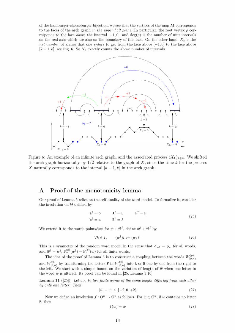
One-endedness. Recall that a graph G = (V,E) is said to be one-ended if for anyfinite subset of vertices U, V\U has exactly one infinite connected component. We willprove that for a word w ∈ W∞, Ψ(w) is one-ended. Let A (resp. ∆) be the arch graph(resp. triangulation) associated to w, and let (M,G) = Ψ(w). By the second conditionin the definition of W∞ (see (24)), there exist arches that connect vertices on the left ofw−R to vertices on the right of wR for any finite number R. Therefore the arch graph Ais one-ended. It is then an easy exercise to deduce from this that the triangulation ∆ andthen the map M are also one-ended.

Recurrence. To prove the recurrence of M we use the general criterion established byGurel-Gurevich and Nachmias [18]. Notice first that under Q(q)

n , the random maps are uni-formly rooted, that is, conditionally on the map, the root vertex ρ is chosen with probabilityproportional to its degree. By [18] it thus suffices to check that the distribution of deg(ρ)has an exponential tail. For this we claim that the variable N0 studied in Lemma 7 exactlycorresponds to the degree of the root in an infinite cFK random map. From the construction

12

of the hamburger-cheeseburger bijection, we see that the vertices of the map M correspondsto the faces of the arch graph in the upper half plane. In particular, the root vertex ρ cor-responds to the face above the interval [−1, 0], and deg(ρ) is the number of unit intervalson the real axis which are also on the boundary of this face. On the other hand, Xk is thenet number of arches that one enters to get from the face above [−1, 0] to the face above[k − 1, k], see Fig. 6. So N0 exactly counts the above number of intervals.

k = −8 k = 0

k = 8

k = 14

X−8 = 0

X0 = 0

X8 = 3

X14 = 0

+0

+1+1

+1+1

−1

N0 = 7

Figure 6: An example of an infinite arch graph, and the associated process (Xk)k∈Z. We shiftedthe arch graph horizontally by 1/2 relative to the graph of X, since the time k for the processX naturally corresponds to the interval [k − 1, k] in the arch graph.

A Proof of the monotonicity lemmaOur proof of Lemma 5 relies on the self-duality of the word model. To formalize it, considerthe involution on Θ defined by

a† = b A† = B F† = F

b† = a B† = A(25)

We extend it to the words pointwise: for w ∈ ΘI , define w† ∈ ΘI by

∀k ∈ I, (w†)k := (wk)† (26)

This is a symmetry of the random word model in the sense that φw† = φw for all words,and w† = w†, P(p)

n (w†) = P(p)n (w) for all finite words.

The idea of the proof of Lemma 5 is to construct a coupling between the words W (p)[0,n)

and W (0)[0,n) by transforming the letters F in W (p)

[0,n) into A or B one by one from the right tothe left. We start with a simple bound on the variation of length of w when one letter inthe word w is altered. Its proof can be found in [25, Lemma 3.10].

Lemma 11 ([25]). Let u, v be two finite words of the same length differing from each otherby only one letter. Then

|u| − |v| ∈ {−2, 0,+2} (27)

Now we define an involution f : Θn → Θn as follows. For w ∈ Θn, if w contains no letterF, then

f(w) = w (28)

13

Otherwise, let k be the index of the last F in w and j = φw(k), and set

f(w) = w†[0,j)w[j,k]w†(k,n) (29)

In the case j = −∞ (that is, wk = F is unmatched), this is the same as f(w) = w[0,k]w†(k,n).

We denote by w(A) the word obtained from w by replacing the last F by A, with the conventionthat w(A) = w if w contains no F. According to Lemma 11, we have

∣∣∣w(A)∣∣∣−|w| ∈ {−2, 0,+2}.

Then f has the following property.

Lemma 12. If∣∣∣w(A)

∣∣∣− |w| = −2, then∣∣∣f(w)(A)

∣∣∣− ∣∣∣f(w)∣∣∣ = +2.

Proof. Assume that∣∣∣w(A)

∣∣∣ − |w| = −2. Then w contains the letter F. Let k be the indexof the last F and j = φw(k). First, we claim that wk is matched and wj 6= a, otherwise wewould have w = w(A). Therefore, wj = b.

By Proposition 3, the word w(j,k) contains no letters which can be matched to either bor F. This implies that w(j,k) = Am for some m ≥ 0. (xm is the word obtained by repeatingthe letter x m times.) Let Uu = w[0,j) such that U contains only uppercase letters andu contains only lowercase letters. In other words, U = w[0,j)

Λ, u = w[0,j)λ. Similarly let

V v = w(k,n). Now we use the property uv = u v (see below Proposition 3) to reduce thewords w and w(A) by block. Write w = w[0,j)bw(j,k)Fw(k,n) and w(A) = w[0,j)bw(j,k)Aw(k,n).Then

w = UubAmFV v = UuAmV v w(A) = UubAmAV v = UubAm+1V v (30)

We have moved U out of the reduction operator since U is “a sequence of orders arriving atthe beginning of the day” and therefore does not participate in the reduction. Idem for v.Remark that the difference

∣∣∣w(A)∣∣∣ − |w| does not depend on U or on v. So without loss of

generality we assume U = v = ∅.We apply the same procedure to f(w) and f(w)(A). It suffices to replace u by u†, and V

by V † in the result. To summarize, we have

w = u AmV f(w) = u† AmV †

w(A) = u b Am+1V f(w)(A) = u† b Am+1 V †(31)

Recall that wk is the last F in w, so there is no F in V or V †. Therefore the four wordson the right-hand side in (31) are of the form xY , where x contains only a and b, and Ycontains only A and B. The length a such word is given by∣∣xY ∣∣ =

∣∣(#a)x− (#A)Y∣∣+∣∣(#b)x− (#B)Y

∣∣ (32)

where (#a)x is the number of letters a in x, idem for the other terms. Set ∆a = (#a)u −(#A)V and ∆b = (#b)u− (#B)V , then (31) gives

|w| = |∆a −m|+ |∆b|∣∣∣f(w)

∣∣∣ = |∆b −m|+ |∆a|∣∣∣w(A)∣∣∣ = |∆a −m− 1|+ |∆b + 1|

∣∣∣f(w)(A)∣∣∣ = |∆b −m− 1|+ |∆a + 1|

(33)

Since∣∣∣w(A)

∣∣∣−|w| = −2, we must have ∆a−m−1 ≥ 0 and ∆b+1 ≤ 0. But m is nonnegative,

so ∆a ≥ 0 and ∆b −m ≤ 0. This implies that∣∣∣f(w)(A)

∣∣∣− ∣∣∣f(w)∣∣∣ = +2.

Proof of Lemma 5. For a random word X taking values in Θn, let Y be the random wordwhich is chosen to be X(A) or X(B) with probability 1/2 independently from X. In otherwords, the mapping X 7→ Y transforms the last letter F in X, if exists, into an A or a B withequal probability. Remark that if we iterate this operation n times on W (p)

[0,n), we obtain a

random word having the same law asW (0)[0,n). Moreover, each intermediate word X generated

during the iteration satisfies f(X) = X in distribution. This can be seen by conditioningon the position of the F’s in the initial word. Therefore, to prove the lemma, it is enough toshow that

∣∣Y ∣∣ ≤st

∣∣X∣∣ for random words X such that f(X) = X in distribution.

14

By Lemma 12, we have for such X

P(∣∣Y ∣∣− ∣∣X∣∣ = −2) =

1

2

(P(∣∣∣X(A)

∣∣∣− ∣∣X∣∣ = −2) + P(∣∣∣X(B)

∣∣∣− ∣∣X∣∣ = −2))

≤ 1

2

(P(∣∣∣f(X)(A)

∣∣∣− ∣∣∣f(X)∣∣∣ = 2) + P(

∣∣∣f(X)(B)∣∣∣− ∣∣∣f(X)

∣∣∣ = 2))

=1

2

(P(∣∣∣X(A)

∣∣∣− ∣∣X∣∣ = 2) + P(∣∣∣X(B)

∣∣∣− ∣∣X∣∣ = 2))

= P(∣∣Y ∣∣− ∣∣X∣∣ = 2)

But, as it is the case for X(A) and X(B), Y differs from X by at most one letter. Therefore∣∣Y ∣∣− ∣∣X∣∣ ∈ {−2, 0,+2} and the above inequality implies that∣∣Y ∣∣ ≤st

∣∣X∣∣.References[1] J. Ambjørn, B. Durhuus, and T. Jonsson. Quantum geometry: a statistical field theory

approach. Cambridge Monographs on Mathematical Physics. Cambridge UniversityPress, Cambridge, 1997.

[2] O. Angel and O. Schramm. Uniform infinite planar triangulations. Comm. Math. Phys.,241(2-3):191–213, 2003. arXiv:math/0207153.

[3] I. Benjamini and O. Schramm. Recurrence of distributional limits of finite planargraphs. Electron. J. Probab., 6:no. 23, 13 pp. (electronic), 2001.

[4] N. Berestycki, B. Laslier, and G. Ray. Critical exponents on fortuin–kastelyn weightedplanar maps. Preprint, 2015. arXiv:1502.00450.

[5] O. Bernardi. Bijective counting of tree-rooted maps and shuffles of parenthesis systems.Electron. J. Combin., 14(1):Research Paper 9, 36 pp. (electronic), 2007.

[6] O. Bernardi and M. Bousquet-Mélou. Counting colored planar maps: algebraicityresults. J. Combin. Theory Ser. B, 101(5):315–377, 2011.

[7] J. E. Björnberg and S. Ö. Stefánsson. Recurrence of bipartite planar maps. Electron.J. Probab., 19:no. 31, 40, 2014. arXiv:1311.0178.

[8] G. Borot, J. Bouttier, and E. Guitter. Loop models on random maps via nested loops:the case of domain symmetry breaking and application to the Potts model. J. Phys.A, 45(49):494017, 35, 2012. arXiv:1207.4878.

[9] G. Borot, J. Bouttier, and E. Guitter. More on the O(n) model on random mapsvia nested loops: loops with bending energy. J. Phys. A, 45(27):275206, 32, 2012.arXiv:1202.5521.

[10] G. Borot, J. Bouttier, and E. Guitter. A recursive approach to the O(n) model onrandom maps via nested loops. J. Phys. A, 45(4):045002, 38, 2012. arXiv:1106.0153.

[11] J. Bouttier, P. Di Francesco, and E. Guitter. Planar maps as labeled mobiles. Electron.J. Combin., 11(1):Research Paper 69, 27, 2004. arXiv:math/0405099.

[12] P. Chassaing and B. Durhuus. Local limit of labeled trees and expected volume growthin a random quadrangulation. Ann. Probab., 34(3):879–917, 2006. arXiv:math/0311532.

[13] N. Curien, L. Ménard, and G. Miermont. A view from infinity of the uniform infiniteplanar quadrangulation. ALEA Lat. Am. J. Probab. Math. Stat., 10(1):45–88, 2013.arXiv:1201.1052.

[14] A. Dembo and O. Zeitouni. Large deviations techniques and applications, volume 38 ofApplications of Mathematics (New York). Springer-Verlag, New York, second edition,1998.

[15] B. Eynard and C. Kristjansen. Exact solution of the O(n) model on a random lattice.Nuclear Phys. B, 455(3):577–618, 1995.

[16] G. Grimmett. The random-cluster model, volume 333 of Grundlehren der Mathema-tischen Wissenschaften [Fundamental Principles of Mathematical Sciences]. Springer-Verlag, Berlin, 2006.

[17] A. Guionnet, V. F. R. Jones, D. Shlyakhtenko, and P. Zinn-Justin. Loop models,random matrices and planar algebras. Comm. Math. Phys., 316(1):45–97, 2012.

15

[18] O. Gurel-Gurevich and A. Nachmias. Recurrence of planar graph limits. Ann. of Math.(2), 177(2):761–781, 2013. arXiv:1206.0707.

[19] E. Gwynne, C. Mao, and X. Sun. Scaling limits for the critical fortuin-kasteleyn modelon a random planar map i: cone times. Preprint, 2015. arXiv:1502.00546.

[20] I. K. Kostov. O(n) vector model on a planar random lattice: spectrum of anomalousdimensions. Modern Phys. Lett. A, 4(3):217–226, 1989.

[21] M. Krikun. Local structure of random quadrangulations. Preprint, 2006.arXiv:math/0512304.

[22] L. Ménard. The two uniform infinite quadrangulations of the plane have the same law.Ann. Inst. Henri Poincaré Probab. Stat., 46(1):190–208, 2010. arXiv:0812.0965.

[23] G. Miermont. Aspects of random maps. Lecture notes of the 2014 Saint-Flour Probabil-ity Summer School, http://perso.ens-lyon.fr/gregory.miermont/coursSaint-Flour.pdf.

[24] G. Schaeffer. Conjugaison d’arbres et cartes combinatoires aléatoires. PhD thesis,Université de Bordeaux 1, 1998.

[25] S. Sheffield. Quantum gravity and inventory accumulation. Preprint, 2011.arXiv:1108.2241.

16