Basic to Reliability Process

Marvin Rausand, March 14, 2006 System Reliability Theory (2nd ed), Wiley, 2004 – 1 / 31

Chapter 2Failure Models

Part 1: Introduction

Marvin Rausand

Department of Production and Quality EngineeringNorwegian University of Science and Technology

[email protected]

http://www.ntnu.no/~marvinr

http://www.ntnu.no/ross/srt

Introduction

Introduction

Rel. measures

Life distributions

State variable

Time to failure

Distr. function

Probability density

Distribution of T

Reliability funct.

Failure rate

Bathtub curve

Some formulas

MTTF

Example 2.1

Median

Mode

MRL

Example 2.2

Discretedistributions

Life distributions




Reliability measures

Introduction

Rel. measures

Life distributions

State variable

Time to failure

Distr. function

Probability density

Distribution of T

Reliability funct.

Failure rate

Bathtub curve

Some formulas

MTTF

Example 2.1

Median

Mode

MRL

Example 2.2


Life distributions


In this chapter we introduce the following measures:

■ The reliability (survivor) function R(t)■ The failure rate function z(t)■ The mean time to failure (MTTF)■ The mean residual life (MRL)

of a single item that is not repaired when it fails.



Life distributions

Introduction

Rel. measures

Life distributions

State variable

Time to failure

Distr. function

Probability density

Distribution of T

Reliability funct.

Failure rate

Bathtub curve

Some formulas

MTTF

Example 2.1

Median

Mode

MRL

Example 2.2


Life distributions


The following life distributions are discussed:

■ The exponential distribution■ The gamma distribution■ The Weibull distribution■ The normal distribution■ The lognormal distribution■ The Birnbaum-Saunders distribution■ The inverse Gaussian distributions

In addition we cover three discrete distributions:

■ The binomial distribution■ The Poisson distribution■ The geometric distribution



State variable

Introduction

Rel. measures

Life distributions

State variable

Time to failure

Distr. function

Probability density

Distribution of T

Reliability funct.

Failure rate

Bathtub curve

Some formulas

MTTF

Example 2.1

Median

Mode

MRL

Example 2.2


Life distributions


X(t)

0t

1

Time to failure, T

Failure

X(t) =

{

1 if the item is functioning at time t0 if the item is in a failed state at time t

The state variable X(t) and the time to failure T will generallybe random variables.



Time to failure

Introduction

Rel. measures

Life distributions

State variable

Time to failure

Distr. function

Probability density

Distribution of T

Reliability funct.

Failure rate

Bathtub curve

Some formulas

MTTF

Example 2.1

Median

Mode

MRL

Example 2.2


Life distributions


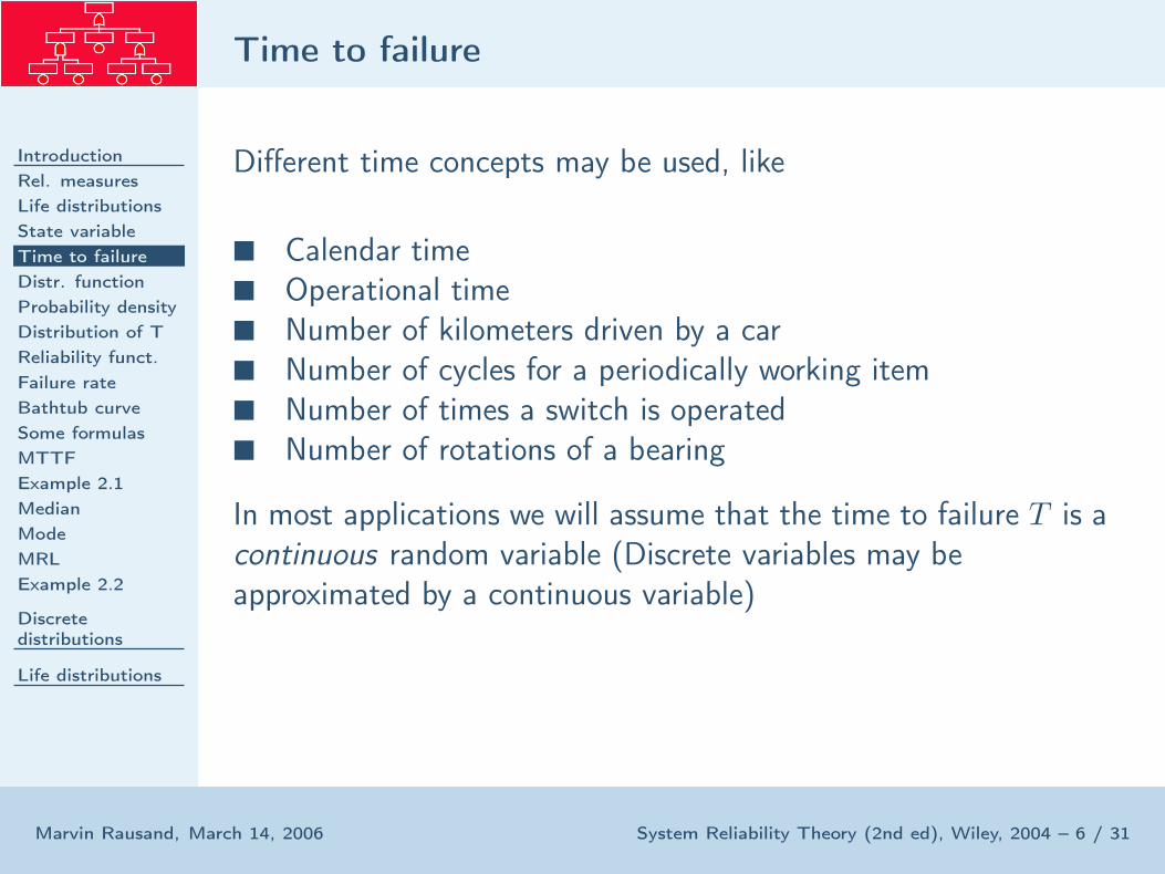
Different time concepts may be used, like

■ Calendar time■ Operational time■ Number of kilometers driven by a car■ Number of cycles for a periodically working item■ Number of times a switch is operated■ Number of rotations of a bearing

In most applications we will assume that the time to failure T is acontinuous random variable (Discrete variables may beapproximated by a continuous variable)



Distribution function

Introduction

Rel. measures

Life distributions

State variable

Time to failure

Distr. function

Probability density

Distribution of T

Reliability funct.

Failure rate

Bathtub curve

Some formulas

MTTF

Example 2.1

Median

Mode

MRL

Example 2.2


Life distributions


The distribution function of T is

F (t) = Pr(T ≤ t) =

∫ t

0f(u) du for t > 0

Note thatF (t) = Probability that the item will fail within the interval (0, t]



Probability density function

Introduction

Rel. measures

Life distributions

State variable

Time to failure

Distr. function

Probability density

Distribution of T

Reliability funct.

Failure rate

Bathtub curve

Some formulas

MTTF

Example 2.1

Median

Mode

MRL

Example 2.2


Life distributions


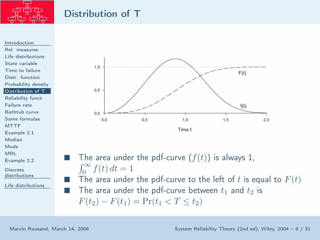
The probability density function (pdf) of T is

f(t) =d

dtF (t) = lim

∆t→∞

F (t + ∆t) − F (t)

∆t= lim

∆t→∞

Pr(t < T ≤ t + ∆

∆t

When ∆t is small, then

Pr(t < T ≤ t + ∆t) ≈ f(t) · ∆t

0 t

∆ t

Time

When we are standing at time t = 0 and ask: What is theprobability that the item will fail in the interval (t, t + ∆t]? Theanswer is approximately f(t) · ∆t



Distribution of T

Introduction

Rel. measures

Life distributions

State variable

Time to failure

Distr. function

Probability density

Distribution of T

Reliability funct.

Failure rate

Bathtub curve

Some formulas

MTTF

Example 2.1

Median

Mode

MRL

Example 2.2


Life distributions


■ The area under the pdf-curve (f(t)) is always 1,∫

∞

0 f(t) dt = 1■ The area under the pdf-curve to the left of t is equal to F (t)■ The area under the pdf-curve between t1 and t2 is

F (t2) − F (t1) = Pr(t1 < T ≤ t2)



Reliability Function

Introduction

Rel. measures

Life distributions

State variable

Time to failure

Distr. function

Probability density

Distribution of T

Reliability funct.

Failure rate

Bathtub curve

Some formulas

MTTF

Example 2.1

Median

Mode

MRL

Example 2.2


Life distributions


R(t) = Pr(T > t) = 1 − F (t) =

∫

∞

tf(u) du

■ R(t) = The probability that the item will not fail in (0, t]■ R(t) = The probability that the item will survive at least to

time t■ R(t) is also called the survivor function of the item



Failure rate function

Introduction

Rel. measures

Life distributions

State variable

Time to failure

Distr. function

Probability density

Distribution of T

Reliability funct.

Failure rate

Bathtub curve

Some formulas

MTTF

Example 2.1

Median

Mode

MRL

Example 2.2


Life distributions


Consider the conditional probability

Pr(t < T ≤ t + ∆t | T > t) =Pr(t < T ≤ t + ∆t)

Pr(T > t)

=F (t + ∆t) − F (t)

R(t)

The failure rate function of the item is

z(t) = lim∆t→0

Pr(t < T ≤ t + ∆t | T > t)

∆t

= lim∆t→0

F (t + ∆t) − F (t)

∆t·

1

R(t)=

f(t)

R(t)

When ∆t is small, we have

Pr(t < T ≤ t + ∆t | T > t) ≈ z(t) · ∆t



Failure Rate Function (2)

Introduction

Rel. measures

Life distributions

State variable

Time to failure

Distr. function

Probability density

Distribution of T

Reliability funct.

Failure rate

Bathtub curve

Some formulas

MTTF

Example 2.1

Median

Mode

MRL

Example 2.2


Life distributions


0 t

∆ t

Time

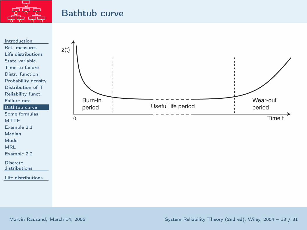
■ Note the difference between the failure rate function z(t) andthe probability density function f(t).

■ When we follow an item from time 0 and note that it is stillfunctioning at time t, the probability that the item will failduring a short interval of length ∆t after time t is z(t) · ∆t

■ The failure rate function is a “property” of the item and issometimes called the force of mortality (FOM) of the item.



Bathtub curve

Introduction

Rel. measures

Life distributions

State variable

Time to failure

Distr. function

Probability density

Distribution of T

Reliability funct.

Failure rate

Bathtub curve

Some formulas

MTTF

Example 2.1

Median

Mode

MRL

Example 2.2


Life distributions


z(t)

Time t0

Burn-in

period Useful life periodWear-out

period



Some formulas

Introduction

Rel. measures

Life distributions

State variable

Time to failure

Distr. function

Probability density

Distribution of T

Reliability funct.

Failure rate

Bathtub curve

Some formulas

MTTF

Example 2.1

Median

Mode

MRL

Example 2.2


Life distributions


Expressed

by F (t) f(t) R(t) z(t)

F (t) = –

Z

t

0

f(u) du 1 − R(t) 1 − exp

„

−

Z

t

0

z(u) du

«

f(t) =d

dtF (t) – −

d

dtR(t) z(t) · exp

„

−

Z

t

0

z(u) du

«

R(t) = 1 − F (t)

Z

∞

t

f(u) du – exp

„

−

Z

t

0

z(u) du

«

z(t) =dF (t)/dt

1 − F (t)

f(t)R

∞

tf(u) du

−

d

dtlnR(t) –



Mean time to failure

Introduction

Rel. measures

Life distributions

State variable

Time to failure

Distr. function

Probability density

Distribution of T

Reliability funct.

Failure rate

Bathtub curve

Some formulas

MTTF

Example 2.1

Median

Mode

MRL

Example 2.2


Life distributions


The mean time to failure, MTTF, of an item is

MTTF = E(T ) =

∫

∞

0tf(t) dt (1)

Since f(t) = −R′(t),

MTTF = −

∫

∞

0tR′(t) dt

By partial integration

MTTF = − [tR(t)]∞0 +

∫

∞

0R(t) dt

If MTTF < ∞, it can be shown that [tR(t)]∞0 = 0. In that case

MTTF =

∫

∞

0R(t) dt (2)

It is often easier to determine MTTF by (2) than by (1).



Example 2.1

Introduction

Rel. measures

Life distributions

State variable

Time to failure

Distr. function

Probability density

Distribution of T

Reliability funct.

Failure rate

Bathtub curve

Some formulas

MTTF

Example 2.1

Median

Mode

MRL

Example 2.2


Life distributions


Consider an item with survivor function

R(t) =1

(0.2 t + 1)2for t ≥ 0

where the time t is measured in months. The probability densityfunction is

f(t) = −R′(t) =0.4

(0.2 t + 1)3

and the failure rate function is

z(t) =f(t)

R(t)=

0.4

0.2 t + 1

The mean time to failure is:

MTTF =

∫

∞

0R(t) dt = 5 months



Median

Introduction

Rel. measures

Life distributions

State variable

Time to failure

Distr. function

Probability density

Distribution of T

Reliability funct.

Failure rate

Bathtub curve

Some formulas

MTTF

Example 2.1

Median

Mode

MRL

Example 2.2


Life distributions


Time t

0 5 10 15 20 25

f(t)

0,00

0,02

0,04

0,06

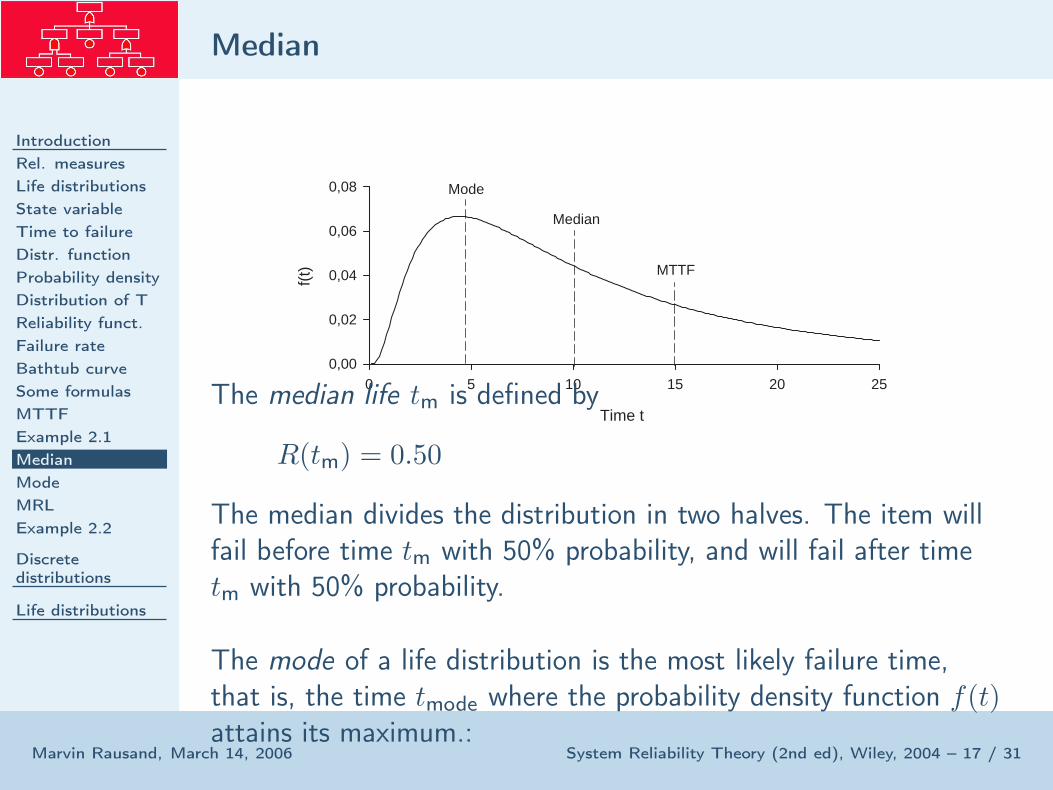
0,08 Mode

Median

MTTF

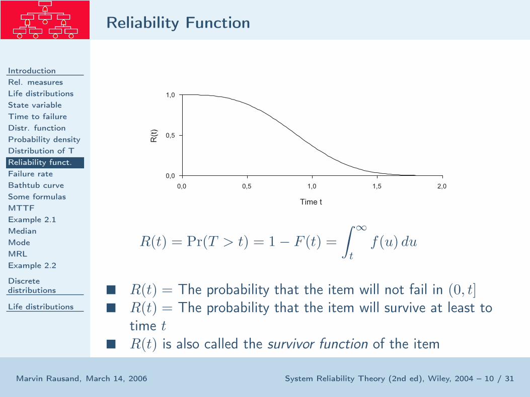
The median life tm is defined by

R(tm) = 0.50

The median divides the distribution in two halves. The item willfail before time tm with 50% probability, and will fail after timetm with 50% probability.

The mode of a life distribution is the most likely failure time,that is, the time tmode where the probability density function f(t)attains its maximum.:



Mode

Introduction

Rel. measures

Life distributions

State variable

Time to failure

Distr. function

Probability density

Distribution of T

Reliability funct.

Failure rate

Bathtub curve

Some formulas

MTTF

Example 2.1

Median

Mode

MRL

Example 2.2


Life distributions


The mode of a life distribution is the most likely failure time,that is, the time tmode where the probability density function f(t)attains its maximum.:



Mean residual life

Introduction

Rel. measures

Life distributions

State variable

Time to failure

Distr. function

Probability density

Distribution of T

Reliability funct.

Failure rate

Bathtub curve

Some formulas

MTTF

Example 2.1

Median

Mode

MRL

Example 2.2


Life distributions


Consider an item that is put into operation at time t = 0 and isstill functioning at time t. The probability that the item of age tsurvives an additional interval of length x is

R(x | t) = Pr(T > x + t | T > t) =Pr(T > x + t)

Pr(T > t)=

R(x + t)

R(t)

R(x | t) is called the conditional survivor function of the item atage t.

The mean residual (or, remaining) life, MRL(t), of the item atage t is

MRL(t) = µ(t) =

∫

∞

0R(x | t) dx =

1

R(t)

∫

∞

tR(x) dx



Example 2.2

Introduction

Rel. measures

Life distributions

State variable

Time to failure

Distr. function

Probability density

Distribution of T

Reliability funct.

Failure rate

Bathtub curve

Some formulas

MTTF

Example 2.1

Median

Mode

MRL

Example 2.2


Life distributions


Consider an item with failure rate function z(t) = t/(t + 1). Thefailure rate function is increasing and approaches 1 when t → ∞.The corresponding survivor function is

R(t) = exp

(

−

∫ t

0

u

u + 1du

)

= (t + 1) e−t

MTTF =

∫

∞

0(t + 1) e−t dt = 2

The conditional survival function is

R(x | t) = Pr(T > x + t | T > t) =(t + x + 1) e−(t+x)

(t + 1) e−t=

t + x + 1

t + 1e

The mean residual life is

MRL(t) =

∫

∞

0R(x | t) dx = 1 +

1

t + 1

We see that MRL(t) is equal to 2 (= MTTF) when t = 0, thatMRL(t) is a decreasing function in t, and that MRL(t) → 1 whent → ∞.



Discrete distributions

Introduction


Binomial

Geometric

Poisson process

Life distributions




Binomial distribution

Introduction


Binomial

Geometric

Poisson process

Life distributions


The binomial situation is defined by:

1. We have n independent trials.2. Each trial has two possible outcomes A and A∗.3. The probability Pr(A) = p is the same in all the n trials.

The trials in this situation are sometimes called Bernoulli trials.Let X denote the number of the n trials that have outcome A.The distribution of X is

Pr(X = x) =

(

n

x

)

px(1 − p)n−x for x = 0, 1, . . . , n

where(

nx

)

= n!x!(n−x)! is the binomial coefficient.

The distribution is called the binomial distribution (n, p), and wesometimes write X ∼ bin(n, p). The mean value and the varianceof X are

E(X) = np var(X) = np(1 − p)



Geometric distribution

Introduction


Binomial

Geometric

Poisson process

Life distributions


Assume that we carry out a sequence of Bernoulli trials, and wantto find the number Z of trials until the first trial with outcome A.If Z = z, this means that the first (z− 1) trials have outcome A∗,and that the first A will occur in trial z. The distribution of Z is

Pr(Z = z) = (1 − p)z−1p for z = 1, 2, . . .

This distribution is called the geometric distribution. We havethat

Pr(Z > z) = (1 − p)z

The mean value and the variance of Z are

E(Z) =1

p

var(X) =1 − p

p2



The homogeneous Poisson process (1)

Introduction


Binomial

Geometric

Poisson process

Life distributions


Consider occurrences of a specific event A, and assume that

1. The event A may occur at any time in the interval, and theprobability of A occurring in the interval (t, t + ∆t] isindependent of t and may be written as λ · ∆t + o(∆t),where λ is a positive constant.

2. The probability of more that one event A in the interval(t, t + ∆t] is o(∆t).

3. Let (t11, t12], (t21, t22], . . . be any sequence of disjointintervals in the time period in question. Then the events “Aoccurs in (tj1, tj2],” j = 1, 2, . . ., are independent.

Without loss of generality we let t = 0 be the starting point ofthe process.



The Homogeneous Poisson Process (2)

Introduction


Binomial

Geometric

Poisson process

Life distributions


Let N(t) denote the number of times the event A occurs duringthe interval (0, t]. The stochastic process {N(t), t ≥ 0} is calleda Homogeneous Poisson Process (HPP) with rate λ.

The distribution of N(t) is

Pr(N(t) = n) =(λt)n

n!e−λt for n = 0, 1, 2, . . .

The mean and the variance of N(t) are

E(N(t)) =∞∑

n=0

n · Pr(N(t) = n) = λt

var(N(t)) = λt



Life distributions

Introduction


Life distributions

Exponential

Weibull




Exponential distribution

Introduction


Life distributions

Exponential

Weibull


Consider an item that is put into operation at time t = 0.Assume that the time to failure T of the item has probabilitydensity function (pdf)

f(t) =

{

λe−λt for t > 0, λ > 00 otherwise

This distribution is called the exponential distribution withparameter λ, and we sometimes write T ∼ exp(λ).

The survivor function of the item is

R(t) = Pr(T > t) =

∫

∞

tf(u) du = e−λt for t > 0

The mean and the variance of T are

MTTF =

∫

∞

0R(t) dt =

∫

∞

0e−λt dt =

1

λ

var(T ) = 1/λ2



Exponential distribution (2)

Introduction


Life distributions

Exponential

Weibull


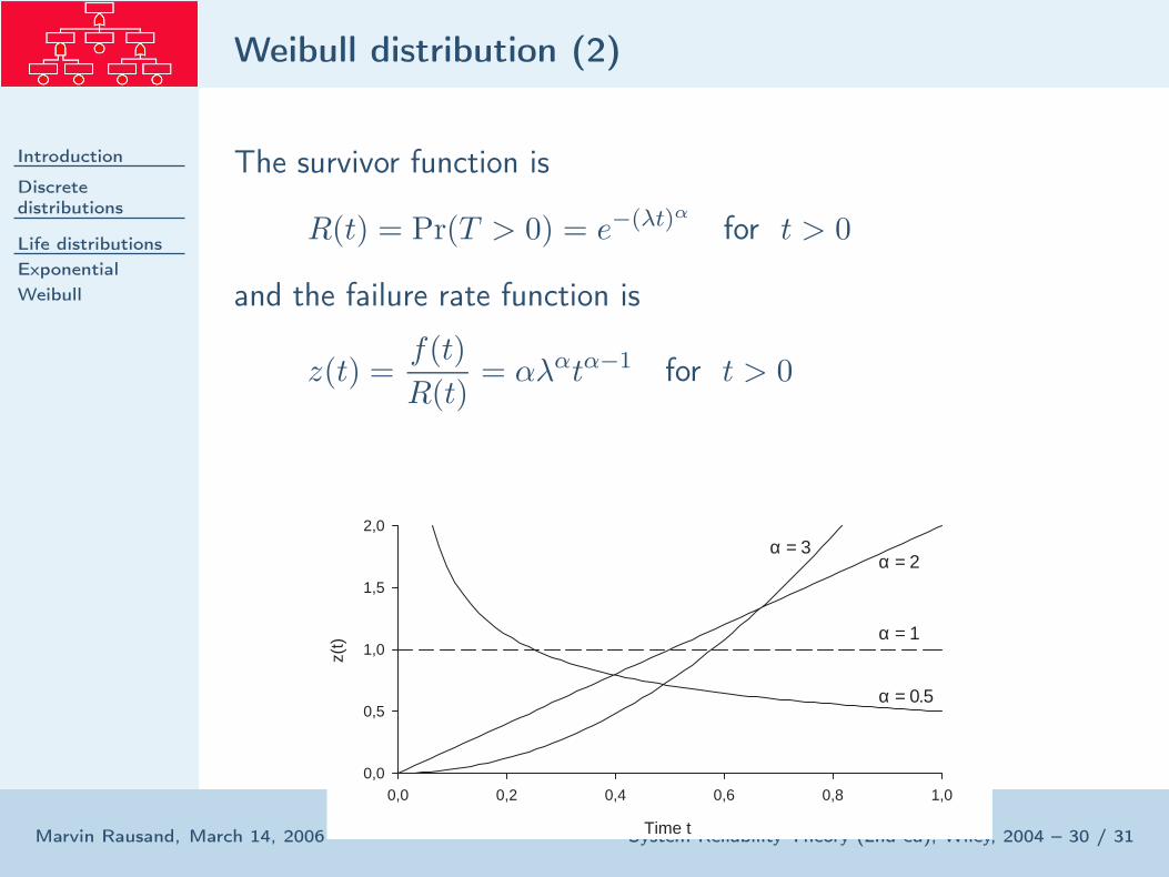
The failure rate function is

z(t) =f(t)

R(t)=

λe−λt

e−λt= λ

The failure rate function is hence constant and independent oftime.Consider the conditional survivor function

R(x | t) = Pr(T > t + x | T > t) =Pr(T > t + x)

Pr(T > t)

=e−λ(t+x)

e−λt= e−λx = Pr(T > x) = R(x)

A new item, and a used item (that is still functioning), willtherefore have the same probability of surviving a time interval oflength t.A used item is therefore stochastically as good as new.



Weibull distribution

Introduction


Life distributions

Exponential

Weibull


The time to failure T of an item is said to be Weibull distributedwith parameters α and λ [T ∼ Weibull(α, λ) ] if the distributionfunction is given by

F (t) = Pr(T ≤ t) =

{

1 − e−(λt)α

for t > 00 otherwise

The corresponding probability density function (pdf) is

f(t) =d

dtF (t) =

{

αλαtα−1e−(λt)α

for t > 00 otherwise

Time t

0,0 0,5 1,0 1,5 2,0 2,5 3,0

f(t)

0,0

0,5

1,0

1,5 α = 0.5

α = 1

α = 2

α = 3



Weibull distribution (2)

Introduction


Life distributions

Exponential

Weibull


The survivor function is

R(t) = Pr(T > 0) = e−(λt)α

for t > 0

and the failure rate function is

z(t) =f(t)

R(t)= αλαtα−1 for t > 0

Time t

0,0 0,2 0,4 0,6 0,8 1,0

z(t)

0,0

0,5

1,0

1,5

2,0

α = 0.5

α = 1

α = 2α = 3



Weibull Distribution (3)

Introduction


Life distributions

Exponential

Weibull


The mean time to failure is

MTTF =

∫

∞

0R(t) dt =

1

λΓ

(

1

α+ 1

)

The median life tm is

R(tm) = 0.50 ⇒ tm =1

λ(ln 2)1/α

The variance of T is

var(T ) =1

λ2

(

Γ

(

2

α+ 1

)

− Γ2

(

1

α+ 1

))

Note that MTTF/√

var(T ) is independent of λ.



Date post:	21-May-2017
Category:	Documents
Upload:	raharjoitb
View:	219 times
Download:	1 times

Basic to Reliability Process

Documents