Basics of epidemiology

Taina Rantanen

Content

• Definition and principles• Research designs and basic concepts• Studying association• Bias• Controlling for confounding• Advances in epidemiology

1.Definition and principles

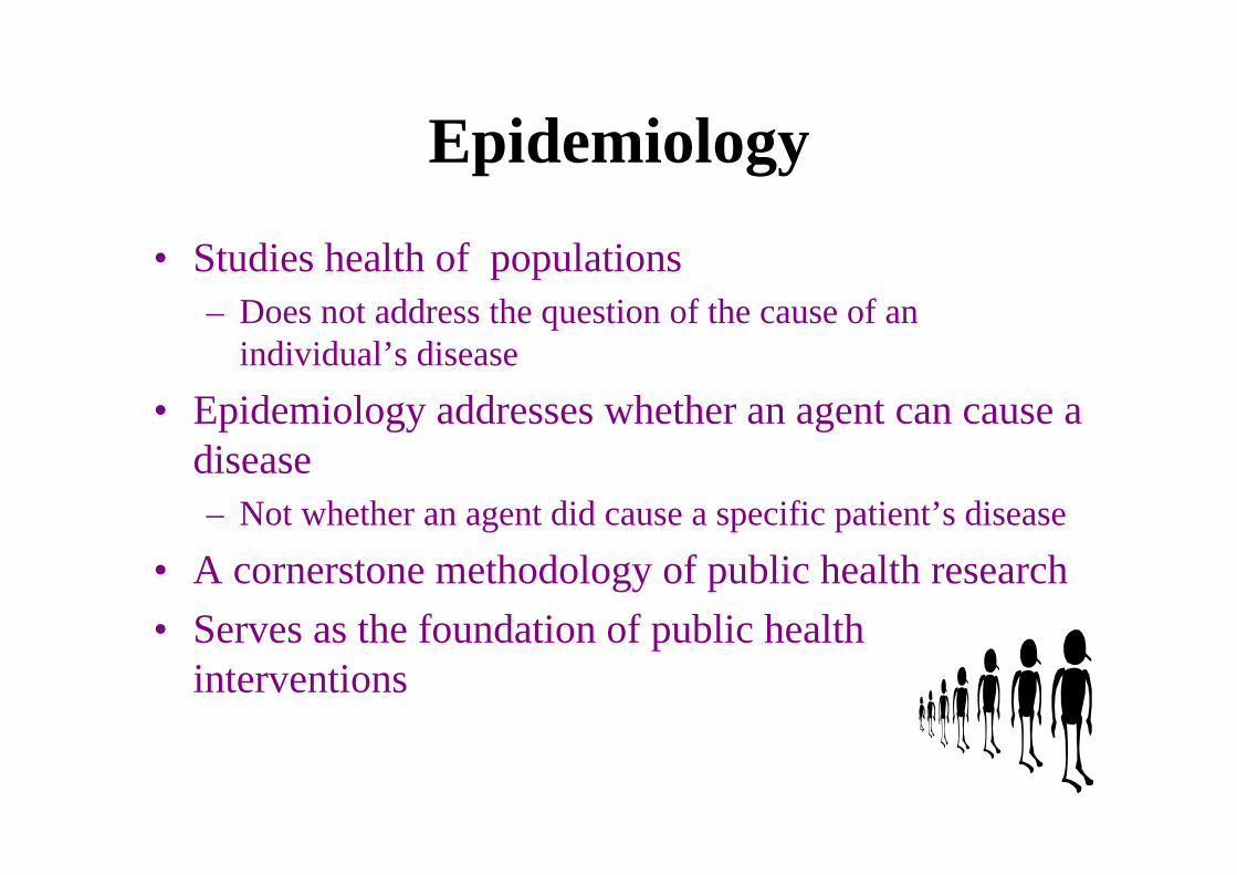
Epidemiology

• Studies health of populations – Does not address the question of the cause of an

individual’s disease

• Epidemiology addresses whether an agent can cause a disease – Not whether an agent did cause a specific patient’s disease

• A cornerstone methodology of public health research• Serves as the foundation of public health

interventions

What can epidemiology do?

• Determine the impact of disease in groups of people. • Detect changes in disease occurrence in groups of people. • Measure relationships between exposure and disease.• Evaluate the efficacy of health interventions and treatments.• Serve as basis for health policy, legislation and resource

allocation– E.g. need for hospital beds, nursing homes, vaccinations…

Non-communicable disease epidemiology• Cardiovascular epidemiology• Cancer epidemiology

Communicable disease epidemiology• HIV/AIDS epidemiology• Infectious disease epidemiology

Environmental epidemiologyOccupational health epidemiologyAging epidemiologyEpidemiology of physical activityGenetic epidemiologyEtc.

Epidemiological methods may be applied to many differentstudy areas

Steps in Performing Research • Research Problem• Literature Review• Conceptual & Theoretical Frameworks• Variables & Hypotheses• Research Design• Population & sample• Data Collection• Data Analysis• Results and findings• Conclusions

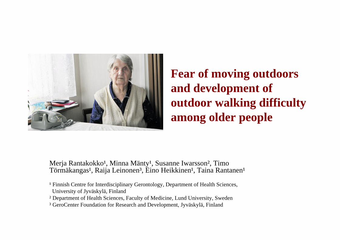
Fear of moving outdoorsand development of outdoor walking difficultyamong older people

Merja Rantakokko¹, Minna Mänty¹, Susanne Iwarsson², Timo Törmäkangas¹, Raija Leinonen³, Eino Heikkinen¹, Taina Rantanen¹

¹ Finnish Centre for Interdisciplinary Gerontology, Department of Health Sciences,University of Jyväskylä, Finland

² Department of Health Sciences, Faculty of Medicine, Lund University, Sweden³ GeroCenter Foundation for Research and Development, Jyväskylä, Finland

Temperature, Humidity, Altitude, Crowding, Housing, Neighborhood,

Water, Radiation,Noise, Air pollution

Age, Sex, Race, Religion, Customs, Occupation, Genetic profile, Marital

status, Family background, Prior diseases, Immune status

Behavioral (malnutrition, physical exercise, smoking, alcohol), Biologic (bacteria, viruses),

Chemical (poison, smoke),Physical (trauma, radiation, fire),

The Epidemiologic Triangle Underlying the Outcome

EnvironmentAgent

Host – individual vulnerability

Introduction

• Fear is a manifestation of subjective lack of safety

• Studies of fear of falling and fear of crime have shown that fears are common among older people, especially among women

• Fear of moving outdoors has not been studied before, even though it may be a factor contributing to the risk of developing mobility limitation in old age

Introduction

• Adapting Tinetti & Powell (1993) definition of fear of falling, our definition of the fear of moving outdoors is:

Fear of moving outdoors is an emotional condition, which can lead to avoidance of outdoor activities, which are well within a person’s functional health capacity

Study questions

• Are there people who have fear of moving outdoors?

• What factors correlate with fear of moving outdoors?

• Does fear of moving outdoors predict development of mobility limitation over a 3.5-year follow-up?

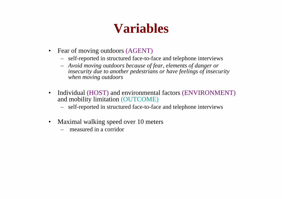
Variables• Fear of moving outdoors (AGENT)

– self-reported in structured face-to-face and telephone interviews– Avoid moving outdoors because of fear, elements of danger or

insecurity due to another pedestrians or have feelings of insecurity when moving outdoors

• Individual (HOST) and environmental factors (ENVIRONMENT)and mobility limitation (OUTCOME)

– self-reported in structured face-to-face and telephone interviews

• Maximal walking speed over 10 meters– measured in a corridor

Participants

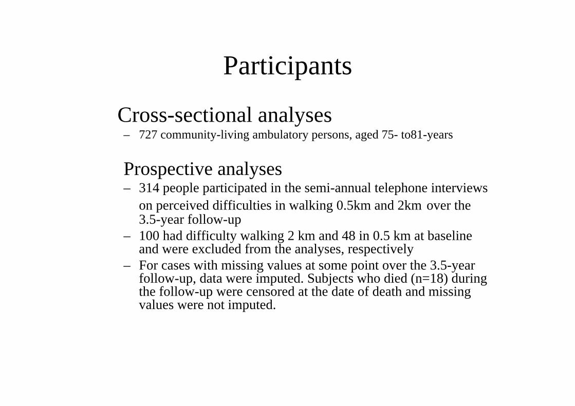
Cross-sectional analyses– 727 community-living ambulatory persons, aged 75- to81-years

Prospective analyses– 314 people participated in the semi-annual telephone interviews

on perceived difficulties in walking 0.5km and 2km over the3.5-year follow-up

– 100 had difficulty walking 2 km and 48 in 0.5 km at baselineand were excluded from the analyses, respectively

– For cases with missing values at some point over the 3.5-year follow-up, data were imputed. Subjects who died (n=18) during the follow-up were censored at the date of death and missing values were not imputed.

Statistical methods

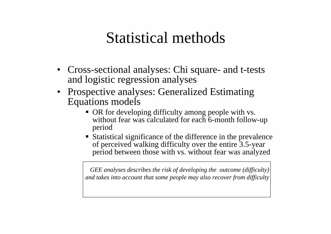
• Cross-sectional analyses: Chi square- and t-testsand logistic regression analyses

• Prospective analyses: Generalized Estimating Equations models

OR for developing difficulty among people with vs. without fear was calculated for each 6-month follow-up periodStatistical significance of the difference in the prevalence of perceived walking difficulty over the entire 3.5-year period between those with vs. without fear was analyzed

GEE analyses describes the risk of developing the outcome (difficulty) and takes into account that some people may also recover from difficulty

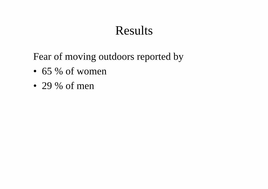
Results

Fear of moving outdoors reported by• 65 % of women• 29 % of men

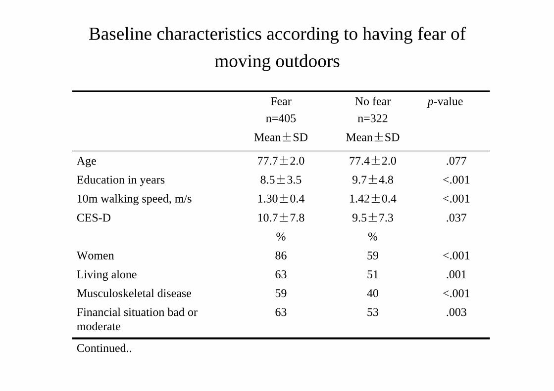
Baseline characteristics according to having fear of moving outdoors

.0035363Financial situation bad ormoderate

p-valueNo fearn=322

Fearn=405

Continued..

<.0014059Musculoskeletal disease.0015163Living alone

<.0015986Women%%

.037 9.5±7.3 10.7±7.8 CES-D<.001 1.42±0.4 1.30±0.4 10m walking speed, m/s<.001 9.7±4.8 8.5±3.5 Education in years.077 77.4±2.0 77.7±2.0 Age

Mean±SD Mean±SD

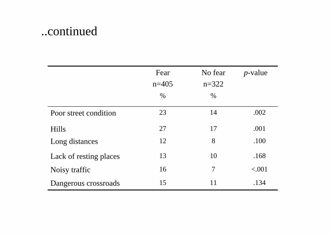
..continued

%%

p-valueNo fearn=322

Fearn=405

.1341115Dangerous crossroads

<.001716Noisy traffic

.1681013Lack of resting places

.100812Long distances

.0011727Hills

.0021423Poor street condition

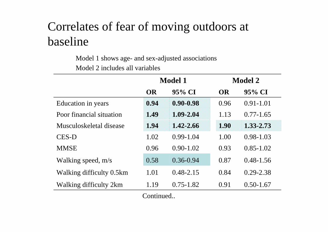
Correlates of fear of moving outdoors at baseline

Model 1 shows age- and sex-adjusted associationsModel 2 includes all variables

0.29-2.380.840.48-2.151.01Walking difficulty 0.5km

0.48-1.560.870.36-0.940.58Walking speed, m/s

Model 1 Model 2OR 95% CI OR 95% CI

Education in years 0.94 0.90-0.98 0.96 0.91-1.01Poor financial situation 1.49 1.09-2.04 1.13 0.77-1.65Musculoskeletal disease 1.94 1.42-2.66 1.90 1.33-2.73CES-D 1.02 0.99-1.04 1.00 0.98-1.03MMSE 0.96 0.90-1.02 0.93 0.85-1.02

Walking difficulty 2km 1.19 0.75-1.82 0.91 0.50-1.67Continued..

..continued

Model 1 Model 2OR 95% CI OR 95% CI

Poor street conditions 1.71 1.13-2.58 1.32 0.81-2.15Hills in the nearby

environment 1.59 1.08-2.32 1.32 0.83-2.10

Long distances 1.36 0.81-2.31 1.18 0.64-2.19

Lack of resting places 1.36 0.84-2.22 1.07 0.58-1.98

Noisy traffic 2.67 1.57-4.56 2.45 1.34-4.48

Dangerous crossroads 1.43 0.90-2.29 1.16 0.66-2.02

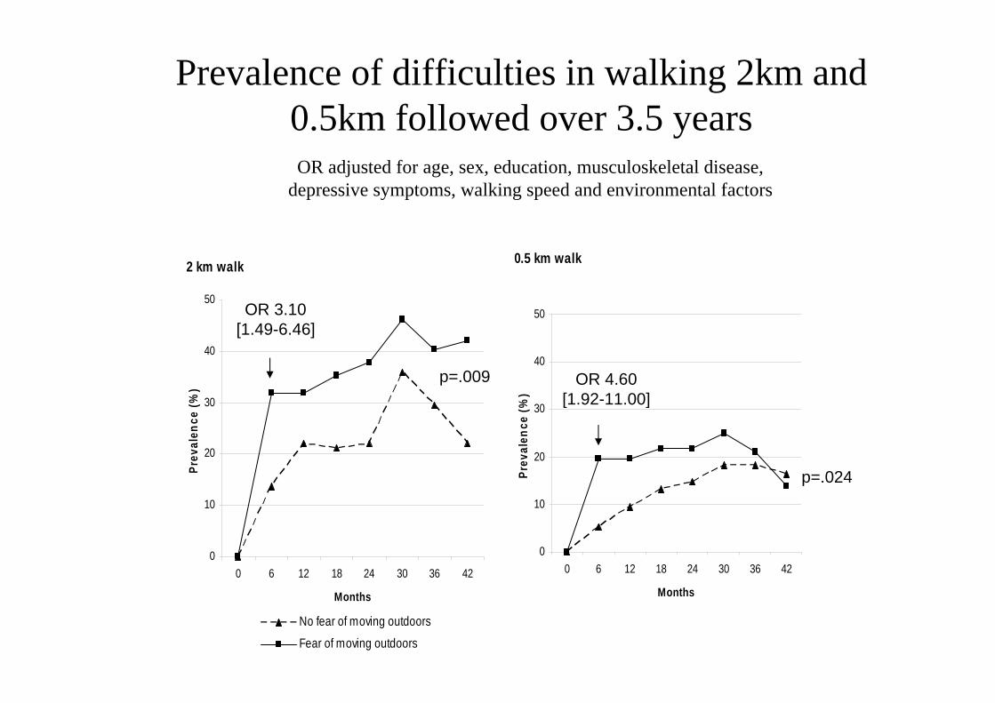
Prevalence of difficulties in walking 2km and 0.5km followed over 3.5 years

0.5 km walk

0

10

20

30

40

50

0 6 12 18 24 30 36 42

Months

Prev

alen

ce (%

)

2 km walk

0

10

20

30

40

50

0 6 12 18 24 30 36 42

Months

Prev

alen

ce (%

)

No fear of moving outdoors

Fear of moving outdoors

OR 3.10[1.49-6.46]

OR 4.60[1.92-11.00]

p=.009

p=.024

OR adjusted for age, sex, education, musculoskeletal disease, depressive symptoms, walking speed and environmental factors

Conclusion

• Fear of moving outdoors is common amongolder adults, especially among women

• Poor socio-economic status, musculoskeletal diseases, slow walking speed and the presence of poor street conditions, hills in the nearby environment and noisy traffic correlated with fear of moving outdoors

• Fear of moving outdoors increases the risk of developing walking difficulties

Conclusion

• Assessment method of fear of moving outdoors warrants further studies

• Environmental design focuses on the objective insecurity, but also subjective insecurity is meaningful for older peoples’ functional capacity

2. Research Designs and Basic Concepts

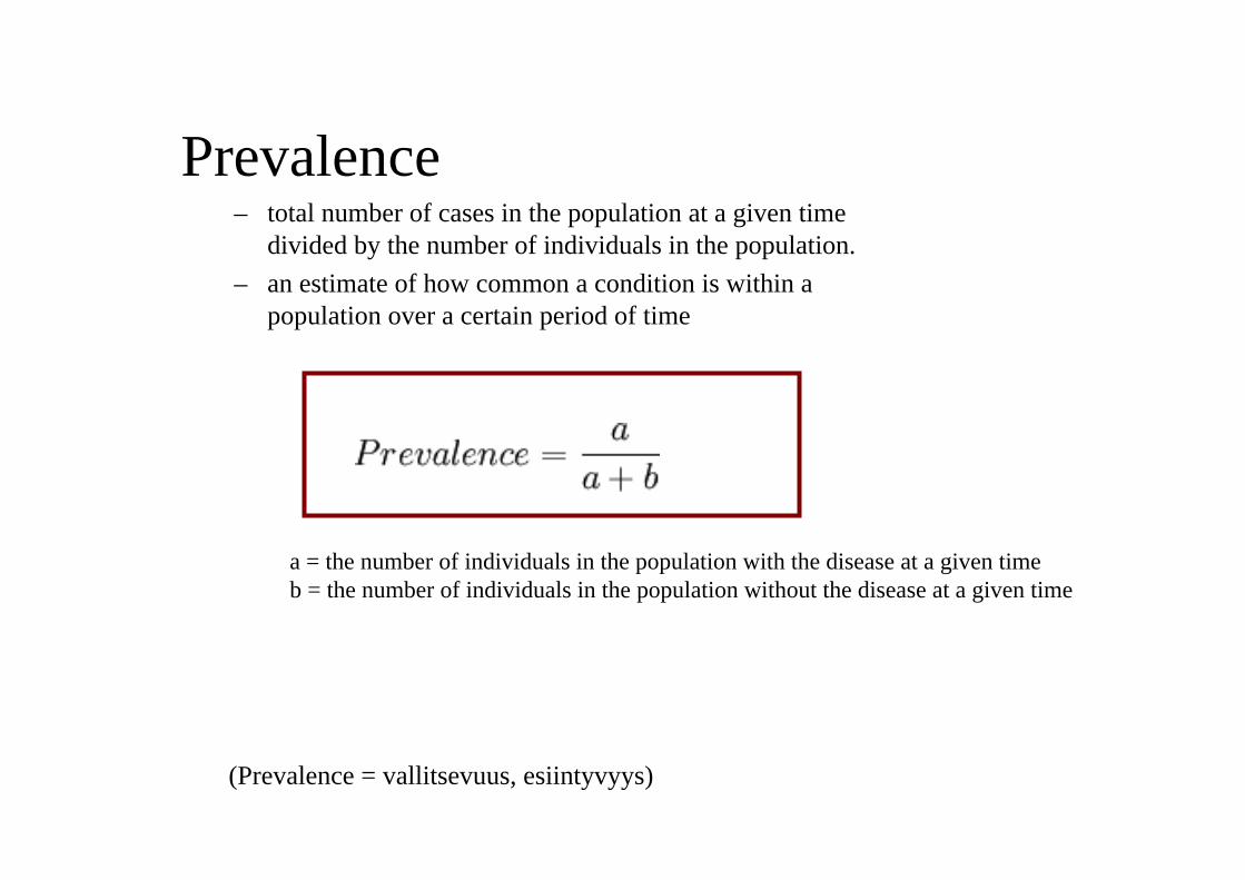
Prevalence – total number of cases in the population at a given time

divided by the number of individuals in the population. – an estimate of how common a condition is within a

population over a certain period of time

a = the number of individuals in the population with the disease at a given timeb = the number of individuals in the population without the disease at a given time

(Prevalence = vallitsevuus, esiintyvyys)

Incidence

– measures the risk of developing a new condition within a specified period of time

– number of new cases during a time period in a population

• We are following a group of 200 initially healthy people over one year. During that time, 50 of them get the disease A. What is incidence of A?

(Incidence = ilmaantuvuus)

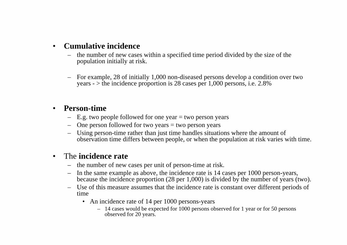
• Cumulative incidence– the number of new cases within a specified time period divided by the size of the

population initially at risk.

– For example, 28 of initially 1,000 non-diseased persons develop a condition over two years - > the incidence proportion is 28 cases per 1,000 persons, i.e. 2.8%

• Person-time– E.g. two people followed for one year = two person years– One person followed for two years = two person years– Using person-time rather than just time handles situations where the amount of

observation time differs between people, or when the population at risk varies with time.

• The incidence rate– the number of new cases per unit of person-time at risk. – In the same example as above, the incidence rate is 14 cases per 1000 person-years,

because the incidence proportion (28 per 1,000) is divided by the number of years (two). – Use of this measure assumes that the incidence rate is constant over different periods of

time• An incidence rate of 14 per 1000 persons-years

– 14 cases would be expected for 1000 persons observed for 1 year or for 50 persons observed for 20 years.

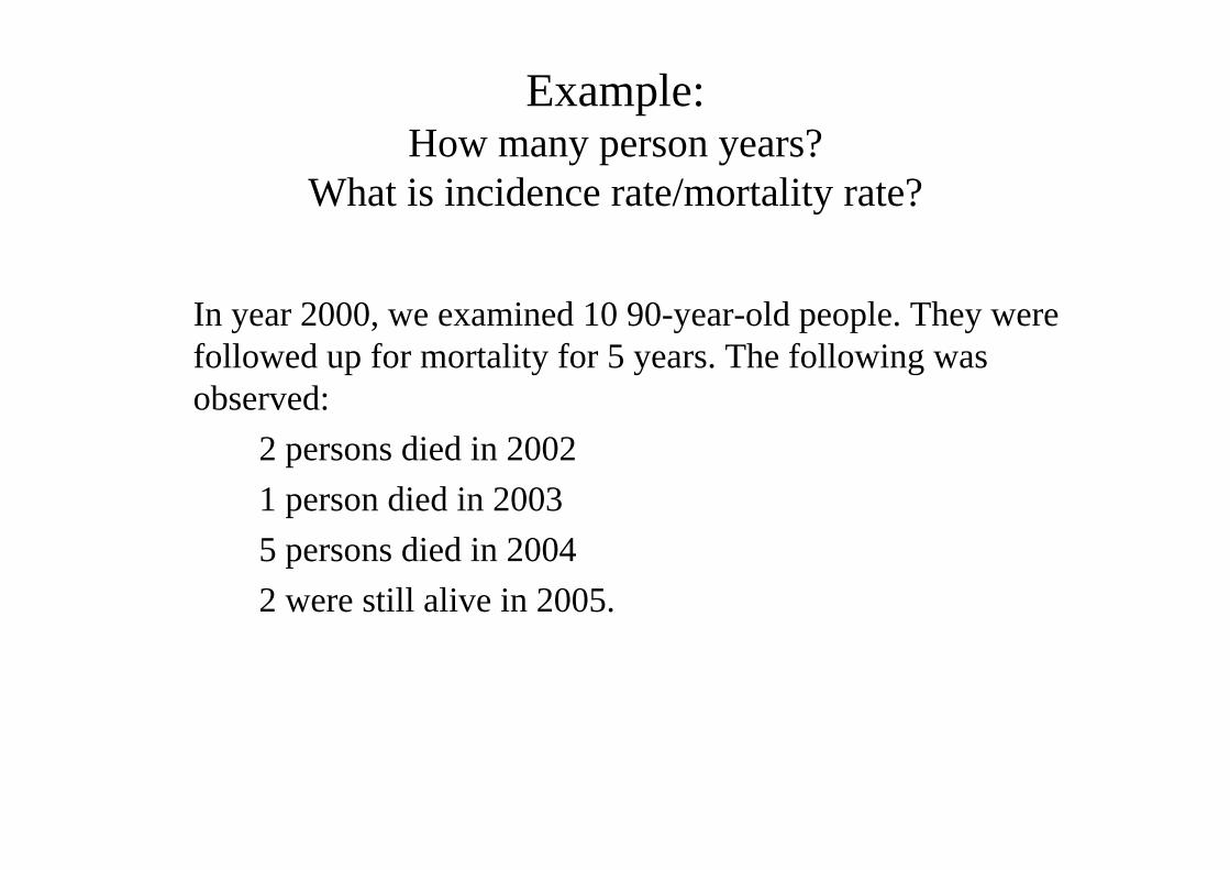
Example: How many person years?

What is incidence rate/mortality rate?

In year 2000, we examined 10 90-year-old people. They werefollowed up for mortality for 5 years. The following wasobserved:

2 persons died in 2002 1 person died in 2003 5 persons died in 2004 2 were still alive in 2005.

Person years:– 2 persons x 2 years = 4– 1 person x 3 years = 4– 5 persons x 4 years = 20– 2 persons x 5 = 10

Sum Total : 38 person years

Mortality rate:8 deaths occured during 38 person years of follow-up

8/38=0.21= 21 deaths/100person-years

8 died

2 survived

Exposure

• Refers to an environmental feature (e.g. pollution, noise, radiation) or a personal habit(e.g. smoking, physical inactivity or activity) which may increase or decrease the risk of the adverse health effect

• In environmental epidemiology exposure refers to contact with an agent through inhalation (breathing chemical vapors), ingestion (swallowing affected food or water) or dermal contact (soaking through skin)

What is an Outcome or Adverse Health Effect?

• Any measurable change in health status, body function or behavior

– For example: symptoms e.g. wheezing or pain, change in immune function, changes in blood chemistry, change in physical fitness, adverse birth outcomes, development of disabilities, clinical disease, and death

Measuring Adverse Health Effects

• Goal: to count all the cases in a particular exposed group or population and compare it with cases in an unexposed group or population

• Where do we get this information?– Death certificates– Registers (e.g. cancer register, hospital discharge

data)– Survey data (self-reports)– Disease biomarkers through direct assessment

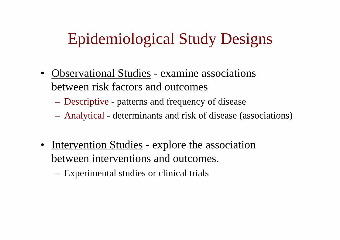
Epidemiological Study Designs

• Observational Studies - examine associations between risk factors and outcomes – Descriptive - patterns and frequency of disease – Analytical - determinants and risk of disease (associations)

• Intervention Studies - explore the association between interventions and outcomes. – Experimental studies or clinical trials

Research Designs in Analytic Epidemiology

• Cohort Study• Case-Control Study• Clinical Trial

Observational

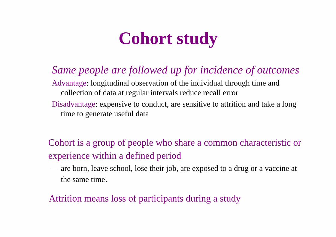
Cohort study

Same people are followed up for incidence of outcomesAdvantage: longitudinal observation of the individual through time and

collection of data at regular intervals reduce recall error Disadvantage: expensive to conduct, are sensitive to attrition and take a long

time to generate useful data

Cohort is a group of people who share a common characteristic orexperience within a defined period– are born, leave school, lose their job, are exposed to a drug or a vaccine at

the same time.

Attrition means loss of participants during a study

Muscle Strength Before andMortality after a Bone Fracture

(Evergreen-project)

BaselineN=493

Knee extension strength

82 fractures32 died

50 alive

Surveillance

No fracturen=411

Fractures 5 years

Mortality 10 years

1,7

15.2

4,9

0

6

12

18

Lowest Middle Highest

Nu m

ber

of D

eat h

s/1 0

00 P

erso

n M

onth

s

Tertiles of Knee Extension Strength Before the Fracture

Mortality Rate after Fracture Accordingto Knee Extension Strength Before the Fracture

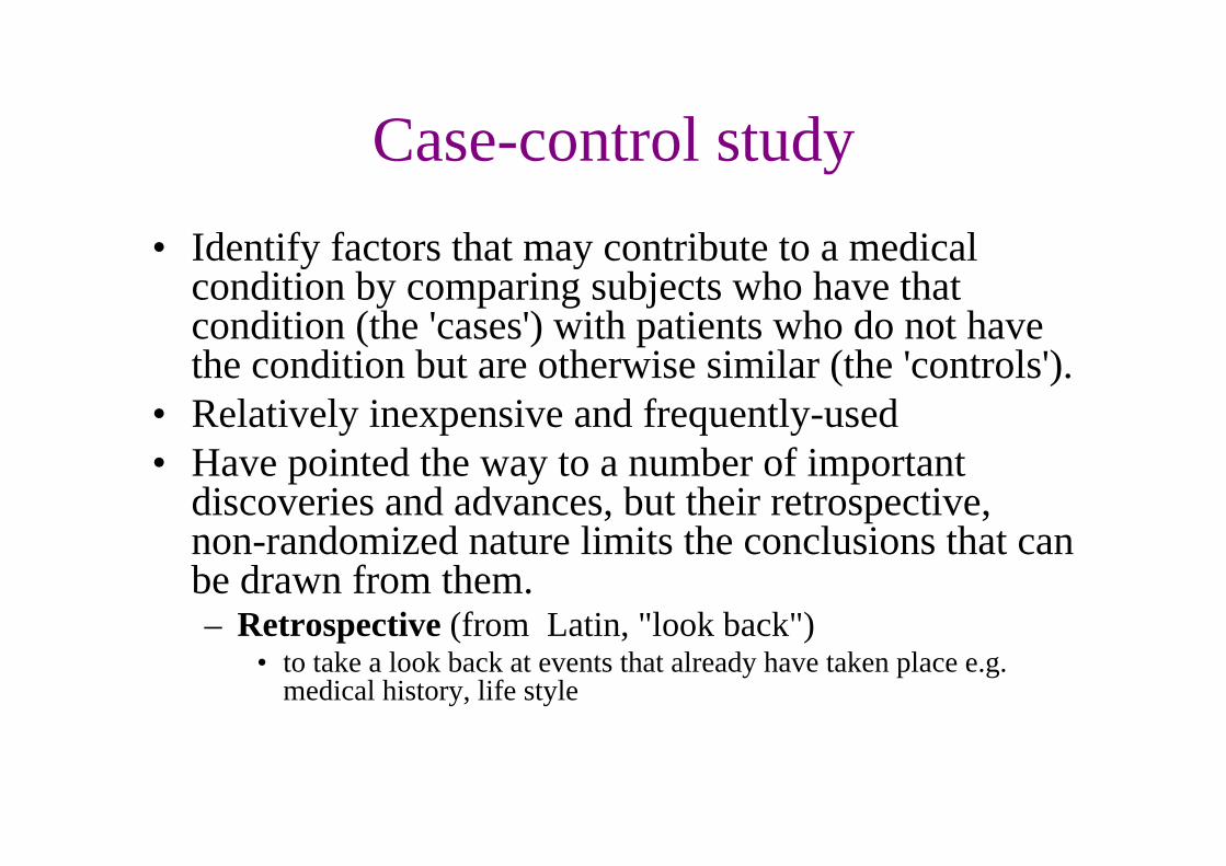
Case-control study• Identify factors that may contribute to a medical

condition by comparing subjects who have that condition (the 'cases') with patients who do not have the condition but are otherwise similar (the 'controls').

• Relatively inexpensive and frequently-used • Have pointed the way to a number of important

discoveries and advances, but their retrospective, non-randomized nature limits the conclusions that can be drawn from them.– Retrospective (from Latin, "look back")

• to take a look back at events that already have taken place e.g.medical history, life style

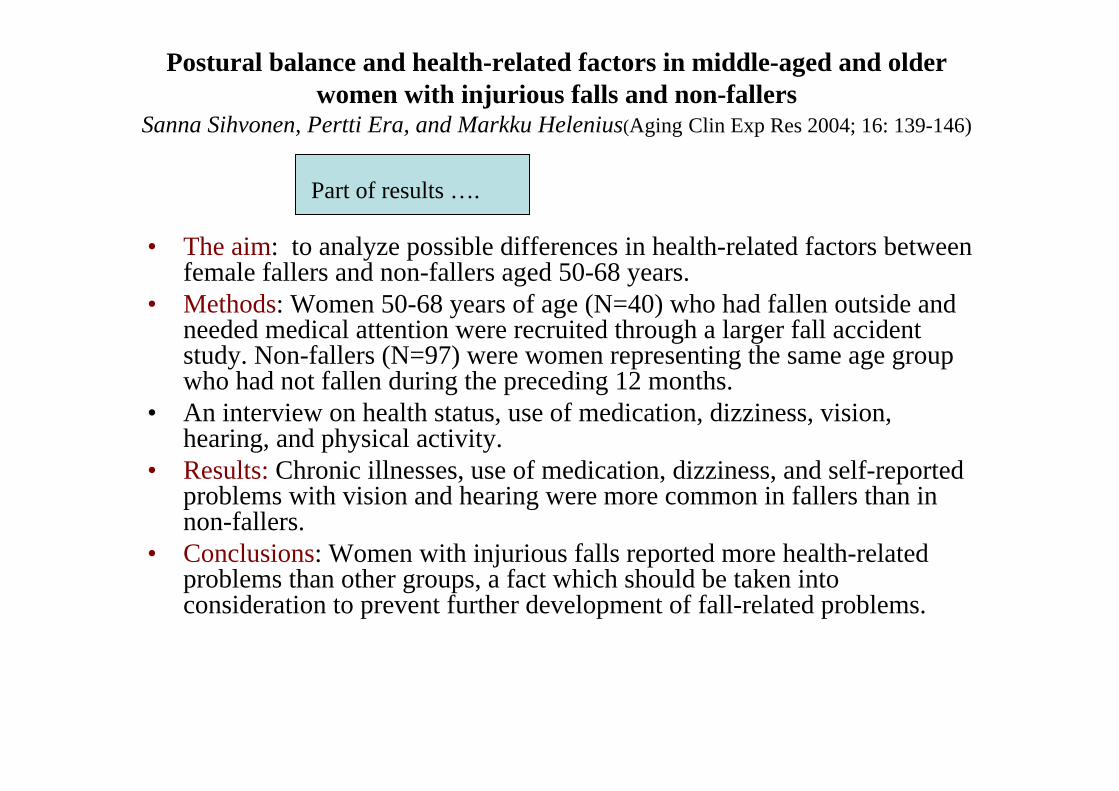
Postural balance and health-related factors in middle-aged and older women with injurious falls and non-fallers

Sanna Sihvonen, Pertti Era, and Markku Helenius(Aging Clin Exp Res 2004; 16: 139-146)

• The aim: to analyze possible differences in health-related factors between female fallers and non-fallers aged 50-68 years.

• Methods: Women 50-68 years of age (N=40) who had fallen outside and needed medical attention were recruited through a larger fall accident study. Non-fallers (N=97) were women representing the same age group who had not fallen during the preceding 12 months.

• An interview on health status, use of medication, dizziness, vision, hearing, and physical activity.

• Results: Chronic illnesses, use of medication, dizziness, and self-reported problems with vision and hearing were more common in fallers than in non-fallers.

• Conclusions: Women with injurious falls reported more health-related problems than other groups, a fact which should be taken into consideration to prevent further development of fall-related problems.

Part of results ….

Clinical trial/ Randomizedcontrolled trial

• Randomized controlled trial (RCT)– tests the efficacy of health care intervention

(pharmaceutical, surgery, medical device, rehabilitation)

– Random allocation of different interventions (treatments or conditions) to subjects ensures that known and unknown confounding factors are evenly distributed between treatment groups.

Common Rates

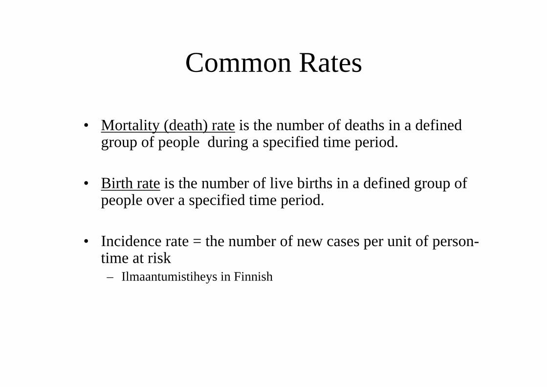
• Mortality (death) rate is the number of deaths in a defined group of people during a specified time period.

• Birth rate is the number of live births in a defined group of people over a specified time period.

• Incidence rate = the number of new cases per unit of person-time at risk– Ilmaantumistiheys in Finnish

3. Studying associations

Common Steps in Establishing a Relationship Between Exposure and Disease

• Physician or other clinicians report series of cases – clinical observation

• Descriptive studies– How common it is?– Who is affected? – Where does it occur?

• Analytic studies– test the exposure-disease hypothesis in a study group

• Disease experimentally reproduced by exposure in animal studies• Observation that removing exposure lowers disease

Measures of Association• How much greater the frequency of disease is in one

group compared with another.

• Often presented in the form of a two-by-two table.

Two-By-Two Table

dc

ba

Disease

Yes No

Yes

Exposure No

Total a+c b+d

Total

a+b

c+d

a+b+c+d

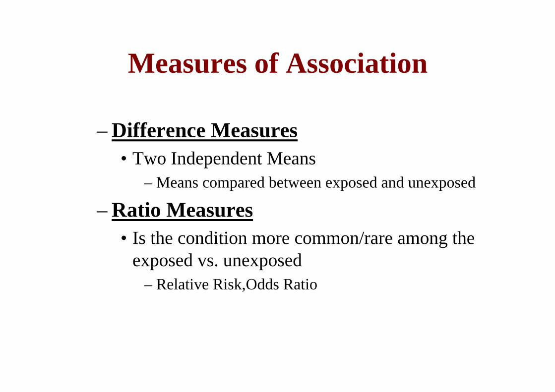
Measures of Association

– Difference Measures• Two Independent Means

– Means compared between exposed and unexposed

– Ratio Measures• Is the condition more common/rare among the

exposed vs. unexposed– Relative Risk,Odds Ratio

Relative Risk (RR)• Measures how likely the exposed group will develop

a disease compared to the unexposed group.

RR = incidence in the exposed incidence in the unexposed

• Population at risk– People who may get the outcome

• For example – Those who are alive may die – Those who do not have the disease yet may get it – Those who have the disease may recover from it– Testicle cancer may develop for men– etc

CHealthyN=40

c case, n=6

Baseline Follow-up

Exposed

Not exposed DHealthyN=60

aCasen=10

b Healthyn= 30

dHealthyN=54

New cases

Prospective cohort study

Incidence of exposed = 10/40=0.25=25%Incidence of unexposed = 6/60 = 0.1 = 10%

Relative Risk (RR) = 25/10= 2.5 Exposed had a 2.5 greater risk than those not exposed

Popu

latio

nat

risk

(N=1

00)

RR of Knee Pain?

At baseline 200 people who did not have knee pain participated. Of them 50% were physically active and 50% sedentary.

At follow-up 10 physically active and 20 sedentarypeople developed knee pain.

Was physical activity associated with knee pain?

BaselineActive n=100 Sedentary n=100

Population at n=100 n=100risk

Follow upNew cases n=10 n=20

Incidence 10/100=0.1 20/100=0.2

Relative risk =0.1/0.2=0.5

Interpretation: Physical activity protected from knee pain

RR < 1 –Protective effectRR > 1 – Increased risk

Example: Calculate mortality ratesand RR of mortality

In 1975, 100 70-year-old people took part in a study. Of them 30 were singing in a choir. 25 years later we collected information about their vital status from population register. Whas singing in a choir associated with mortality risk?

Baseline 1975Singers(n=30) Reference group(n=70)

Years of death f Yrs Prsn-yrs f Yrs Prsn-yrs1977 1 2 2 3 2 61980 5 5 25 20 5 801985 4 10 40 40 10 4001995 10 15 150 2 15 30 2000 1 20 20 4 20 80

Died 21 69Alive in 2000 9 25 225 1 20 20

Prs.yrs Sum 462 616

mortality rate 21/462 =0.045=5/100prs-yrs 69/616=0.11=11/100pers-yrsRR= 4.5/11=0.40Singing in a choir protects from mortality

Exercise:In 1975 1000 70-year old people (60 % women) took part in a survey about driving. Of men 50% and of women 30% had a driving licence.

Revocation of the driving licence had happened as follows

Year Men Womenf f

1980 20 151985 30 201990 40 30

The rest still had their driving licences in 1990Was gender associated with revocation of the driving licence?

Population at risk Men N=200 Women N= 180Person-years till revocation

1980 20 x5 =100 15 x 5 =751985 30 x 10 =300 20x10=2001990 40x 15=600 30 x 15=450Still driving in 1990 110 x 15=1650 115x15=1725

Henk v. 2650 2450Tapauksia 90 65

3.34/100 hv 2.65/100 hv

3.34/2. 65=1.26Men had 26% greater risk for revocation of driving licence

Censoring event• The person is no more at risk of getting the outcome

or leaves the follow up

• In case of mortality, the cencoring event is the deathand the person is cencored at the date of death

• In case of studying disease incidence, the person maydie before getting the disease. In that case cencoringhappens at the death date.

Retrospective studies: case-control studies

• Cases - Has condition or health outcome of interest. Has higher frequency or greater degree of exposure than non-cases.

• Controls (non-cases) - Does not have the health condition. Serves as the comparison group

Exposure• Interview about exposure or use available documents about exposure (e.g.

clinical data, registers, knowledge of work environment)

• If controls are well chosen, the only difference will be in the level of a characteristic that is related causally to the development of a disease (I.e, exposure to a chemical resulted in cancer).

• Quantify with odds ratios

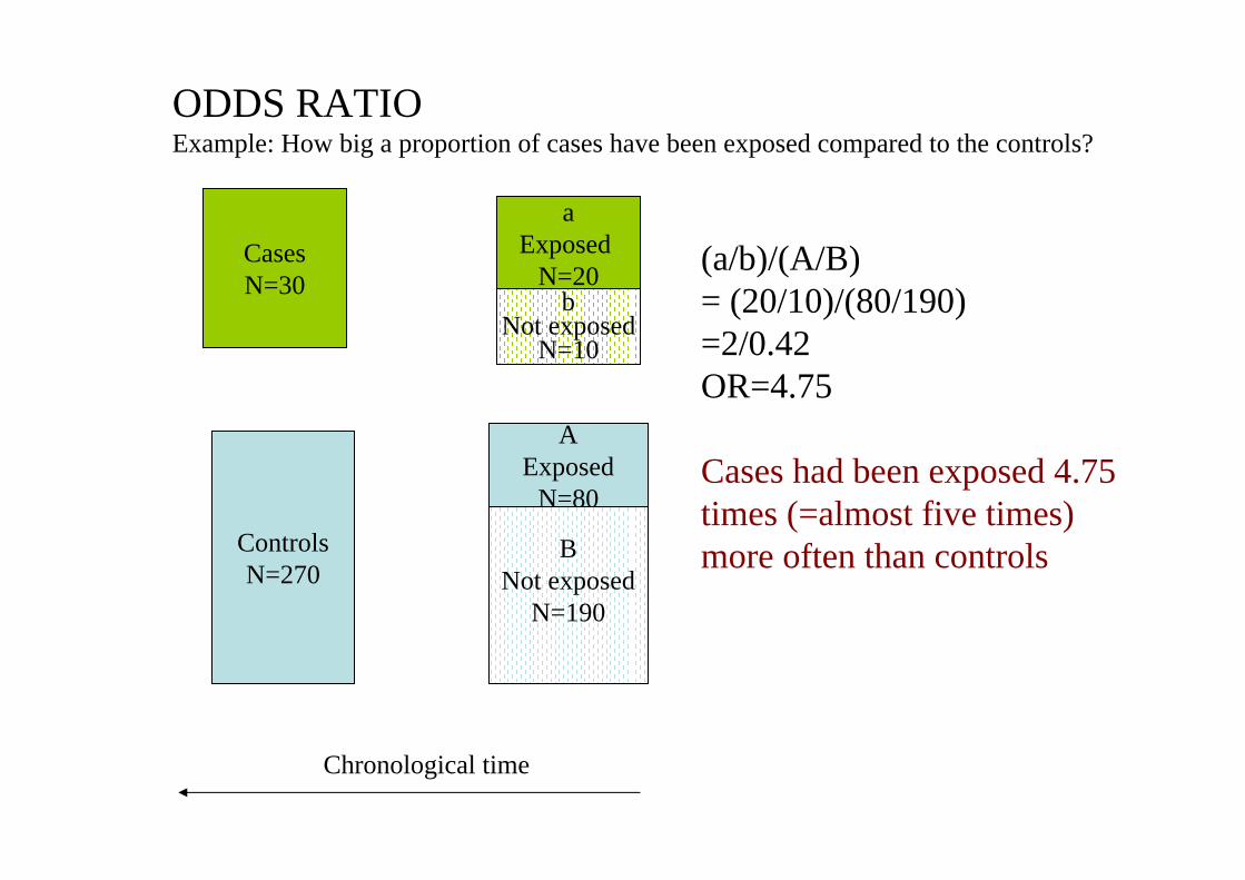
CasesN=30

ControlsN=270

aExposed

N=20

AExposed

N=80

BNot exposed

N=190

bNot exposed

N=10

ODDS RATIOExample: How big a proportion of cases have been exposed compared to the controls?

(a/b)/(A/B) = (20/10)/(80/190)=2/0.42OR=4.75

Cases had been exposed 4.75 times (=almost five times) more often than controls

Chronological time

Example: Does going to restaurant explain breathing difficulties?

Twenty people came to student health center because of for breathing difficulty. In an interview, it was observed that that15 of them had been in Restaurant PartyNight during the previous weekend.

Of the 40 people who had a dentist’s appointment and no breathing difficulty, 20 had been in the PartyNight during he previous weekend.

Is there an association for breathing difficulty and going to Partynight, and if so, is it strong or not?

• (Exposed cases/Unexposed cases)/(Exposed controls/Unexposed controls)

= (15/5)/(20/20)=3/1=3

• People having breathing difficulty had been 3 times more ofthen in PartyNight than those not having breathing difficulty

• Association is strong

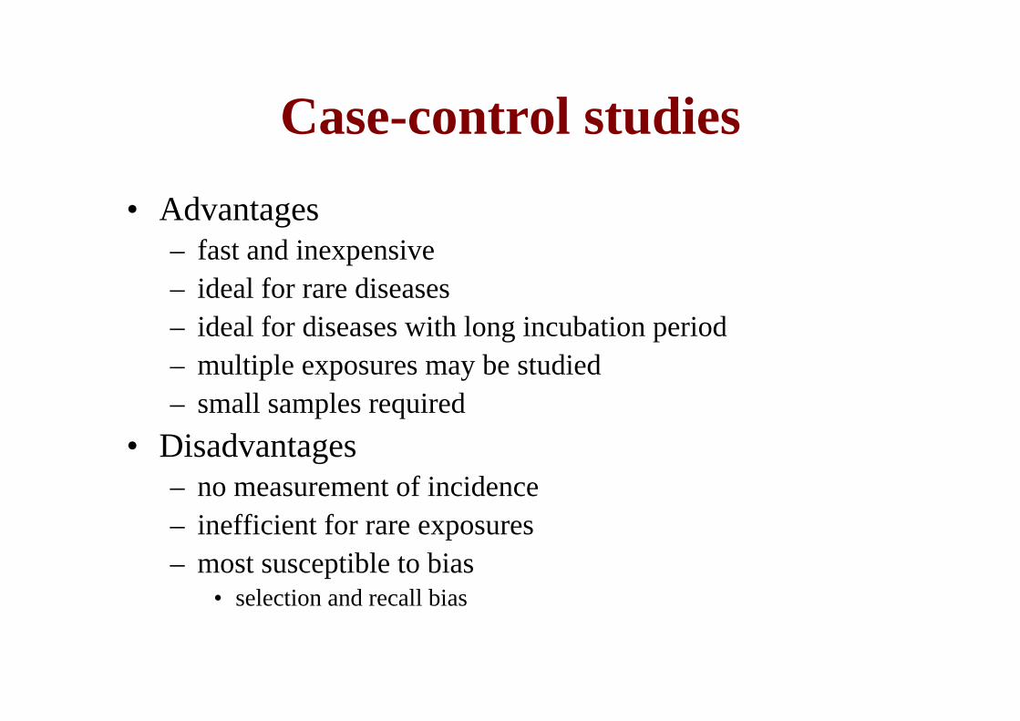
Case-control studies• Advantages

– fast and inexpensive– ideal for rare diseases– ideal for diseases with long incubation period– multiple exposures may be studied– small samples required

• Disadvantages– no measurement of incidence– inefficient for rare exposures– most susceptible to bias

• selection and recall bias

Measures of Association &Hypothesis Testing

Test Statistic =Observed Association - Expected Association

Standard Error of the Association

• Type I Error: Concluding there is an association when one does not exist

• Type II Error: Concluding there is no association when one does exist

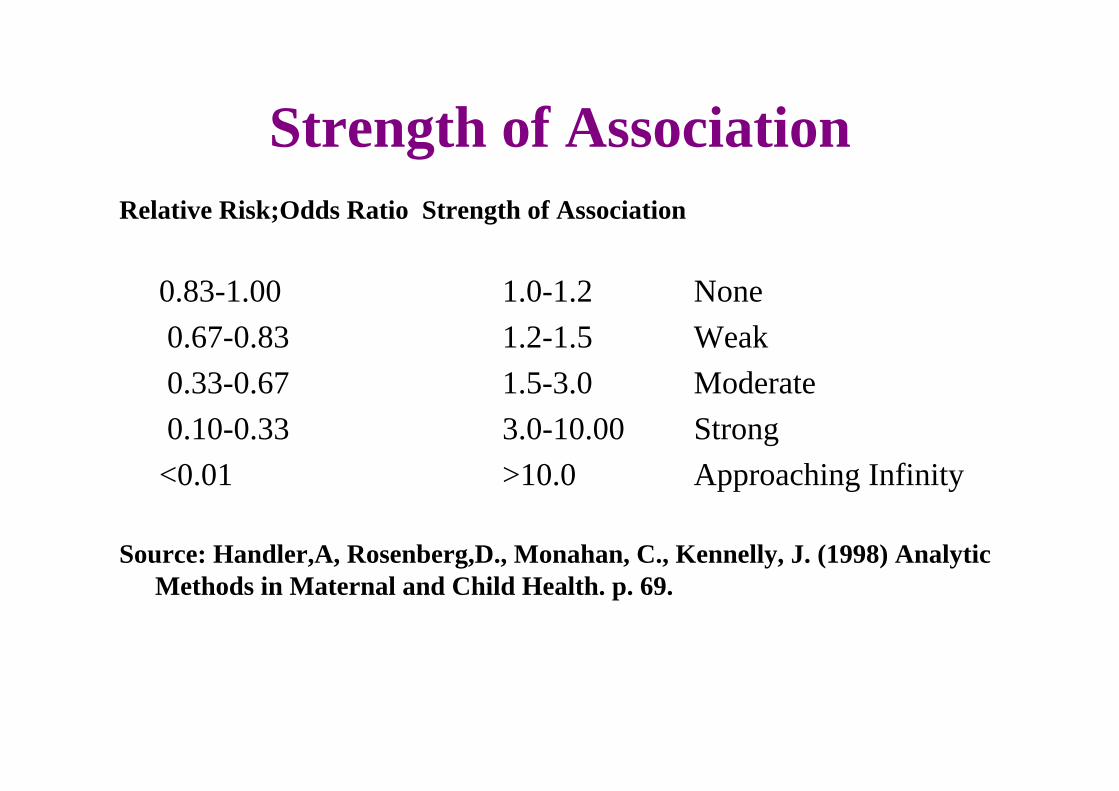
Strength of AssociationRelative Risk;Odds Ratio Strength of Association

0.83-1.00 1.0-1.2 None0.67-0.83 1.2-1.5 Weak0.33-0.67 1.5-3.0 Moderate0.10-0.33 3.0-10.00 Strong<0.01 >10.0 Approaching Infinity

Source: Handler,A, Rosenberg,D., Monahan, C., Kennelly, J. (1998) Analytic Methods in Maternal and Child Health. p. 69.

Causation• 1965 Austin Bradford Hill detailed criteria for assessing evidence of

causation (Bradford-Hill criteria)

– Strength: A small association does not mean that there is not a causal effect.– Consistency: Consistent findings observed by different persons in different

places with different samples strengthens the likelihood of an effect.– Specificity: Causation is likely if a very specific population at a specific site

and disease with no other likely explanation. The more specific an association between a factor and an effect is, the bigger the probability of a causal relationship.

– Temporality: The effect has to occur after the cause (and if there is an expected delay between the cause and expected effect, then the effect must occur after that delay).

– Biological gradient: Greater exposure should generally lead to greater incidence of the effect.

– Plausibility: A plausible mechanism between cause and effect is helpful – Coherence: Coherence between epidemiological and laboratory findings

increases the likelihood of an effect. – Experiment: "Occasionally it is possible to appeal to experimental evidence“– Analogy: The effect of similar factors may be considered

• To study the association in prospective designs->calculate Relative Risk– ”The risk of outcome was x times greater among those with

the exposure compared to those without exposure”

• To study the association is reprospective or cross-sectional designs ->calculate Odds Ratio– ”Those with outcome had x times more often been exposed

(to Z) than those without outcome”

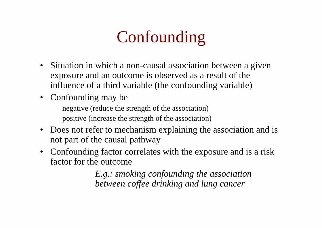
Confounding• Situation in which a non-causal association between a given

exposure and an outcome is observed as a result of the influence of a third variable (the confounding variable)

• Confounding may be– negative (reduce the strength of the association) – positive (increase the strength of the association)

• Does not refer to mechanism explaining the association and is not part of the causal pathway

• Confounding factor correlates with the exposure and is a riskfactor for the outcome

E.g.: smoking confounding the association between coffee drinking and lung cancer

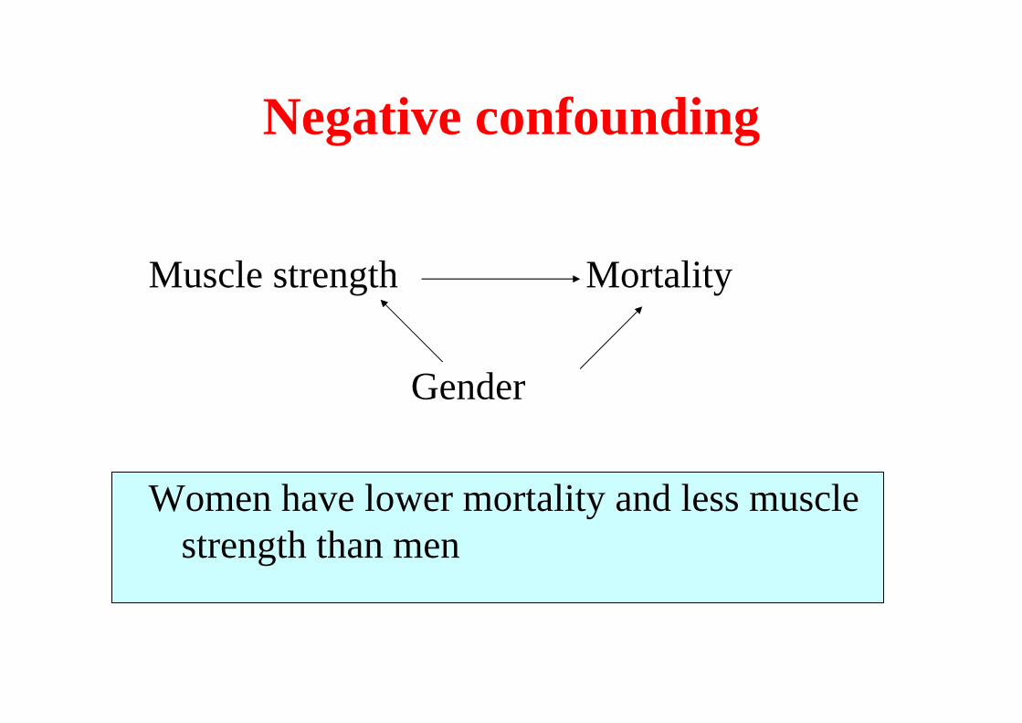
Negative confounding

Muscle strength Mortality

Gender

Women have lower mortality and less musclestrength than men

Positive confounding

Muscle strength Mortality

Age

Older people have higher mortality and lower musclestrength than younger people

Interaction

• Effect modification• Situation when 2 or more risk factors modify

the effect of each other with regard to the occurrence or level of a given outcome

0

5

10

15

20

25

30

35

No Minor Major

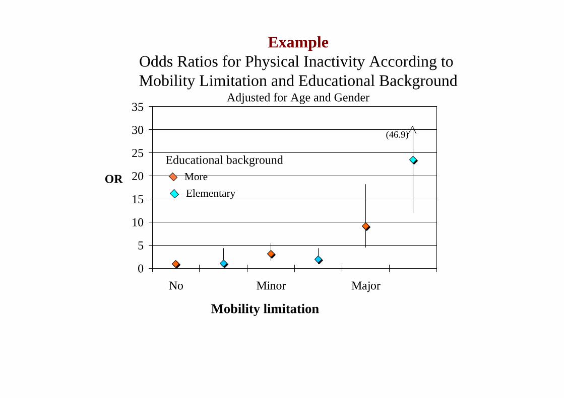
(46.9)

ORElementaryMore

Mobility limitation

ExampleOdds Ratios for Physical Inactivity According to Mobility Limitation and Educational Background

Adjusted for Age and Gender

Educational background

Interpretation• Mobility limitation increases the probability for physical

inactivity, particularly among people with short educationalbackground, an indicator of low socio-economic status– They experience more barriers to physical activity participation, such

as • Lack of financial and social resources• Fears• Poor health• Negative attitutes• Negative environment

Risk factors

• Characteristics associated with increased risk of disease

Cause

• Event or condition or characteristic that plays an essential role in the occurrence of disease– Necessary cause: presence of x necessarily implies the presence of y.

(i.e. chromosomal mutation which always results in a disease, such as Down’s syndrome)

– Sufficient cause: presence of x implies the presence of y. However, another cause z may alternatively cause y. (i.e. smoking and lung cancer, which may happen to also non-smoking people)

• Cause occurs prior to disease in time• Change in cause frequency - >change in disease frequency• Association not due to correlation to another factor• Plausible explanation

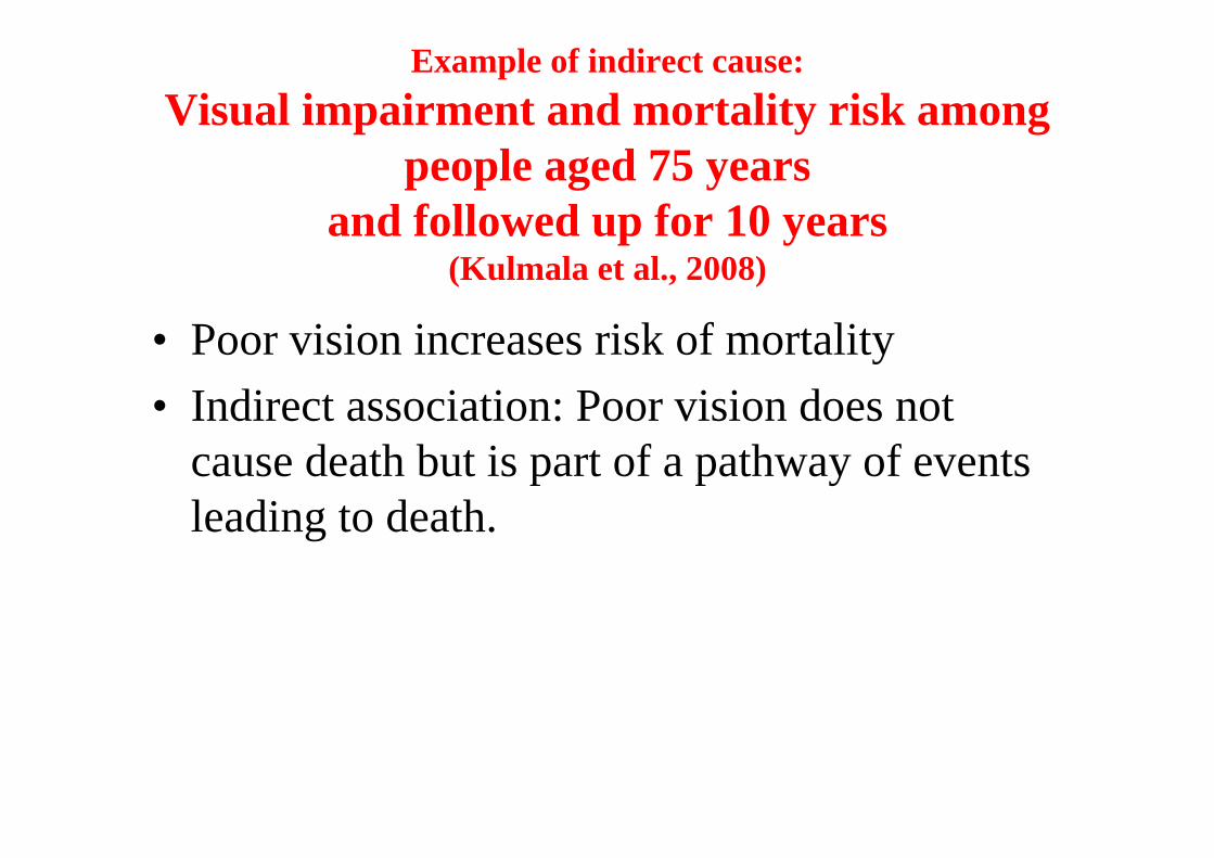
Example of indirect cause:Visual impairment and mortality risk among

people aged 75 yearsand followed up for 10 years

(Kulmala et al., 2008)

• Poor vision increases risk of mortality• Indirect association: Poor vision does not

cause death but is part of a pathway of eventsleading to death.

Indirect causation

Diabetes, CVD

Mortality riskincreases

Vison declines

Phys activity declinesRisk of acccidentsincrease

Aging

Depressive symptomsincrease

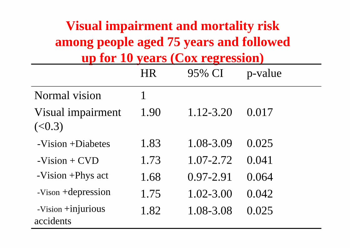
Visual impairment and mortality riskamong people aged 75 years and followed

up for 10 years (Cox regression)

1.12-3.20 0.01711.90

Normal vision Visual impairment(<0.3)

1.08-3.09 0.0251.07-2.72 0.0410.97-2.91 0.0641.02-3.00 0.0421.08-3.08 0.025

1.831.731.681.751.82

-Vision +Diabetes

-Vision + CVD-Vision +Phys act

-Vison +depression

-Vision +injuriousaccidents

95% CI p-valueHR

Bias

• Systematic error which results in estimates that depart systematically from the true value

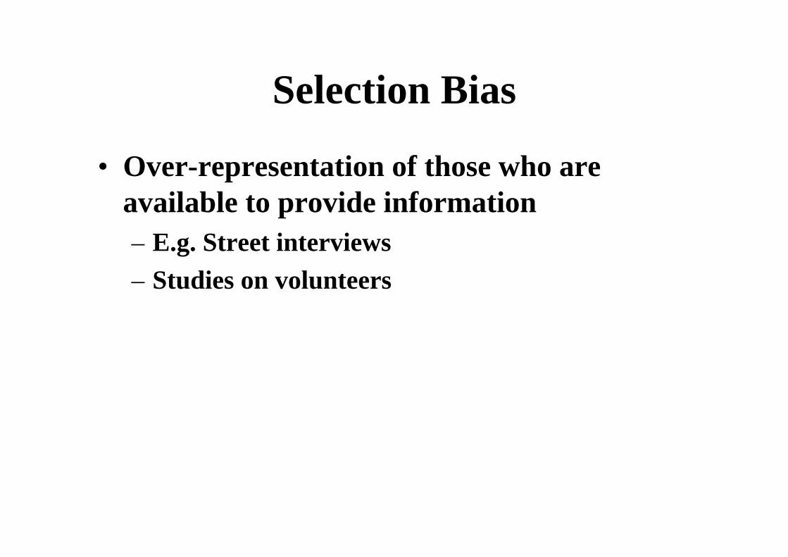
Selection Bias

• Over-representation of those who are available to provide information– E.g. Street interviews– Studies on volunteers

Survivor Bias

• Obtaining data only from those who have survived to provide it– Sicker people are likely to drop out– E.g. studies on centenarians do not provide

information about predictors of survival

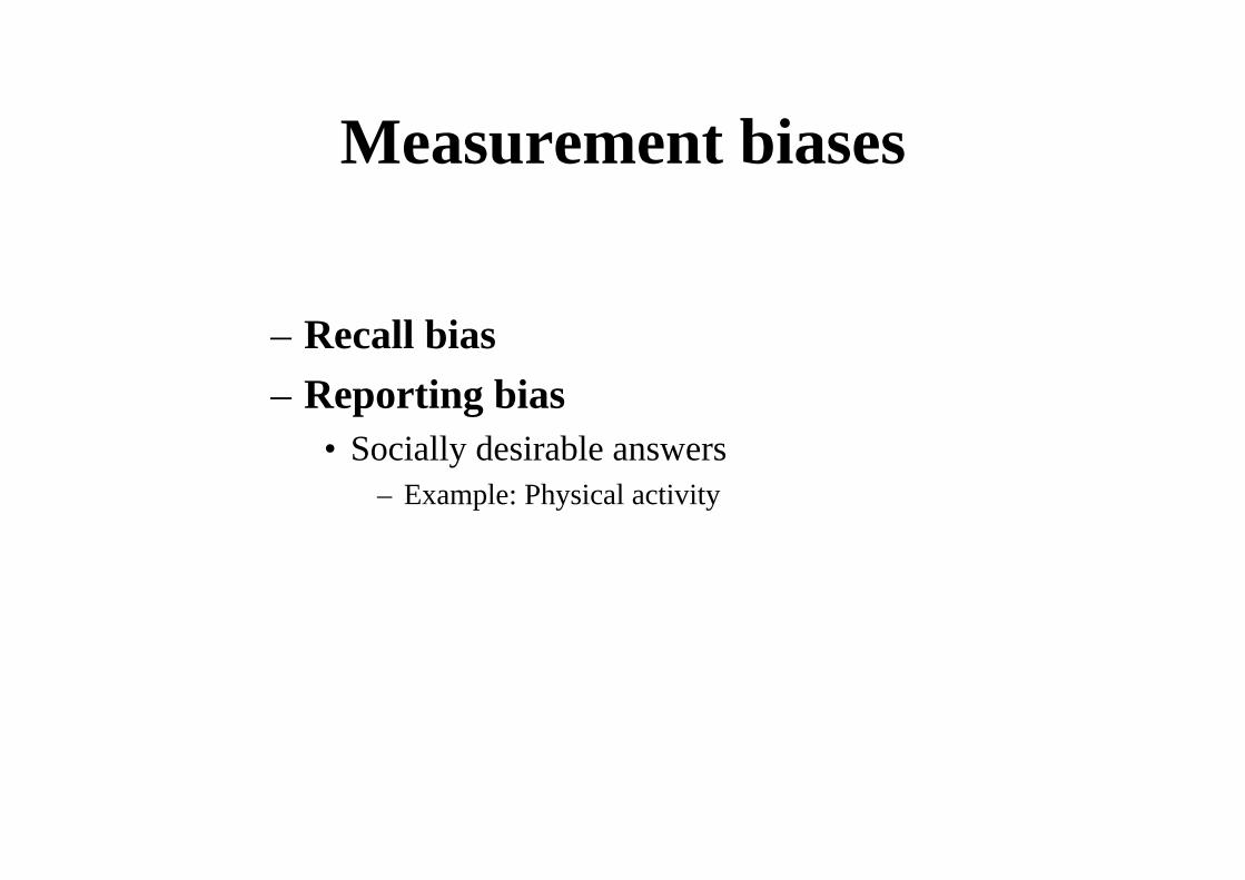
– Recall bias – Reporting bias

• Socially desirable answers– Example: Physical activity

Measurement biases

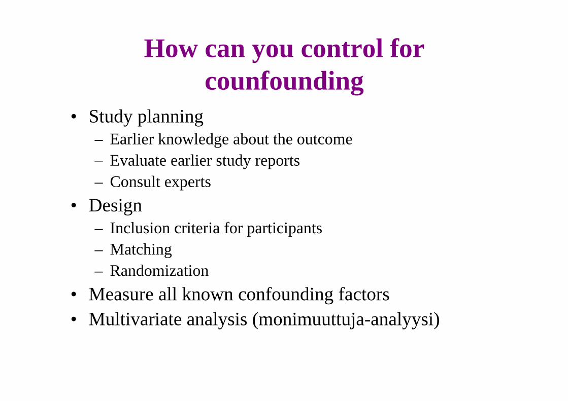
How can you control for counfounding

• Study planning– Earlier knowledge about the outcome– Evaluate earlier study reports– Consult experts

• Design– Inclusion criteria for participants– Matching– Randomization

• Measure all known confounding factors• Multivariate analysis (monimuuttuja-analyysi)

Advances in epidemiology

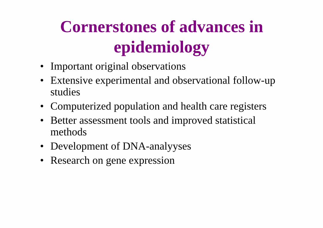
Cornerstones of advances in epidemiology

• Important original observations• Extensive experimental and observational follow-up

studies• Computerized population and health care registers• Better assessment tools and improved statistical

methods• Development of DNA-analyyses• Research on gene expression

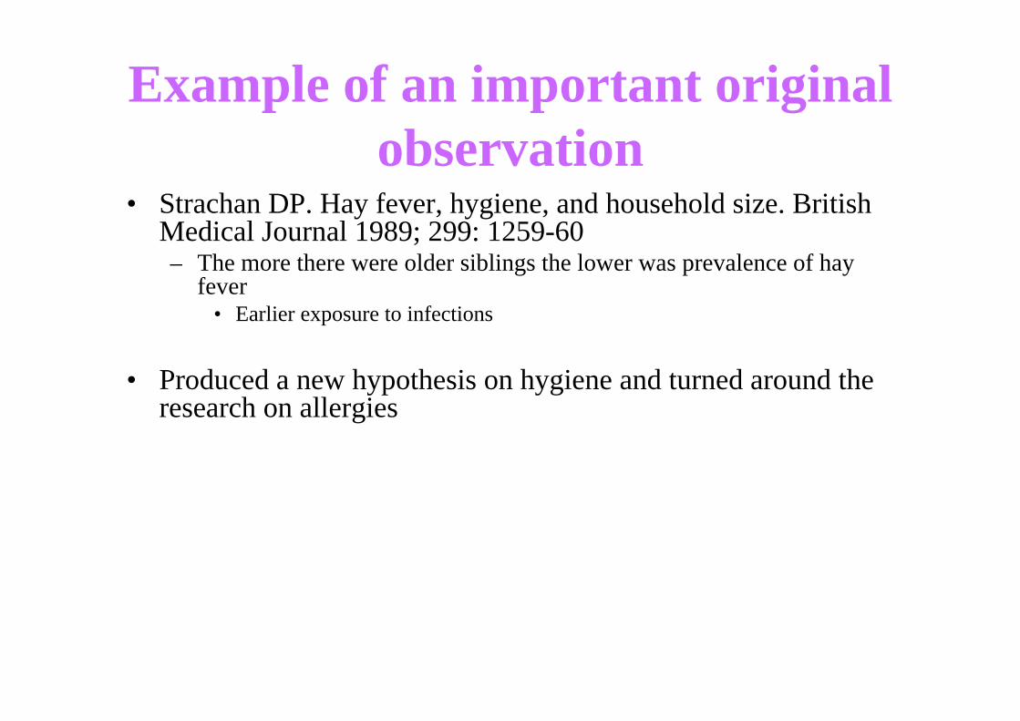
Example of an important originalobservation

• Strachan DP. Hay fever, hygiene, and household size. British Medical Journal 1989; 299: 1259-60– The more there were older siblings the lower was prevalence of hay

fever• Earlier exposure to infections

• Produced a new hypothesis on hygiene and turned around the research on allergies

Genetic epidemiology• First wave – Estimate heritability of phenotypes (diseases or

other traits)

• Search for genes underlying this phenotype

– In case, there are many associated genes and each gene has a smallinfluence, really large data sets are required

• After the relevant genes and their expression are known, it is possible to start to develop new better targetic medicines

GENETIC SELECTION BIAS IN STUDIES ON AGING AND

UNFAVOURABLE GENES

LOW FITNESS LEVEL,DIFFUCULT TO EXERCISE

HIGH MORBIDITY,

PREMATURE AGING

UNFAVOURABLE RISKFACTOR PROFILE

Twin studies

• 1. Answer to the question: How big a proportion of individual differences areexplained by genetic and environmentalfactors

• 2. Allow to study effects of an exposure in a genetically controlled situation

• Finnish Twin Study on Aging– 217 female twin pairs aged 63-76 years

• 103MZ, 114 DZ

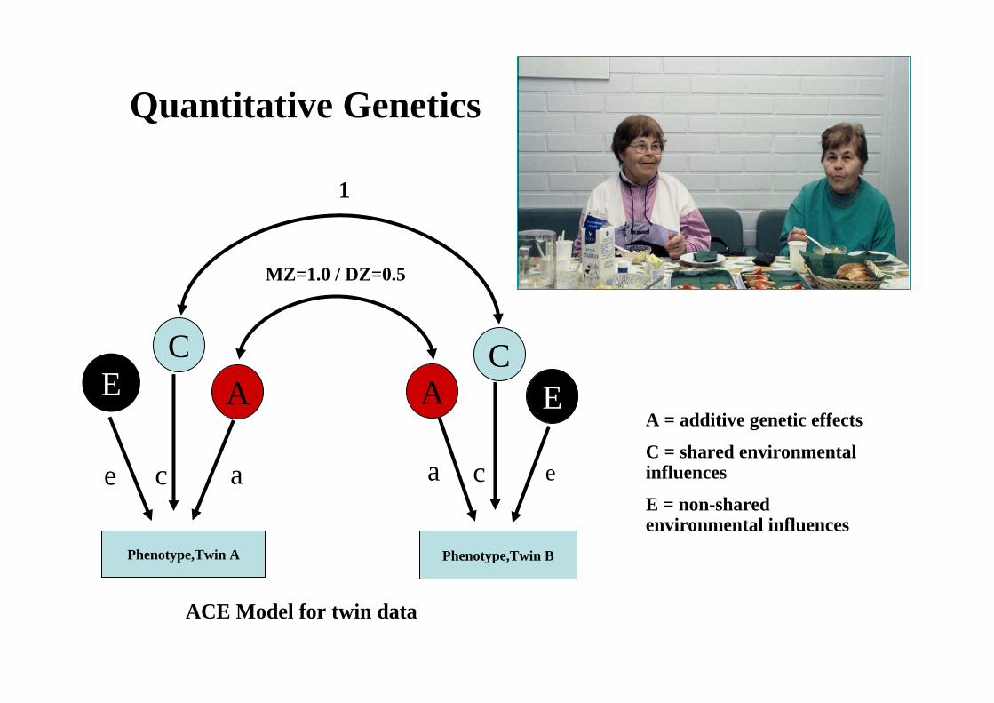
ACE Model for twin data

EA = additive genetic effects

C = shared environmental influences

E = non-shared environmental influences

Phenotype,Twin A

AC

Phenotype,Twin B

AC

E

1

MZ=1.0 / DZ=0.5

e ac ca e

Quantitative Genetics

A Additive genetic effectsC Shared environmental effectsE Individual environmental effects

Same genes underlie individual differences in hand gripand knee extension strength

ISOMETRIC MUSCLE

STRENGTH

LEG EXTENSOR POWERMUSCLE CSA

Ac Ec

As1 Cs4

7%(1-15%)

51% (39-62%)

37% (25-49%)

60% (48-70%)

38% (30-48%)

5%(0-14%)

35%(23-47%)

MAXIMAL WALKING SPEED

Cc

3%(1-8%)

49%(38-61%)

26%(16-36%)

3%(1-7%)

Es4Es1 Es3

25% (18-34%)

34% (27-43%)

27% (16-39%)

ISOMETRIC MUSCLE

STRENGTH

LEG EXTENSOR POWERMUSCLE CSA

Ac Ec

As1 Cs4

7%(1-15%)

51% (39-62%)

37% (25-49%)

60% (48-70%)

38% (30-48%)

5%(0-14%)

35%(23-47%)

MAXIMAL WALKING SPEED

Cc

3%(1-8%)

49%(38-61%)

26%(16-36%)

3%(1-7%)

Es4Es1 Es3

25% (18-34%)

34% (27-43%)

27% (16-39%)

A Additive genetic effectsC Shared environmental effectsE Individual environmental effects

(Tiainen et al. 2008)

What underlies the association of muscle CSA, strength, power and walking speed?

Same genes predispose people to poor strength and power and low walking speed

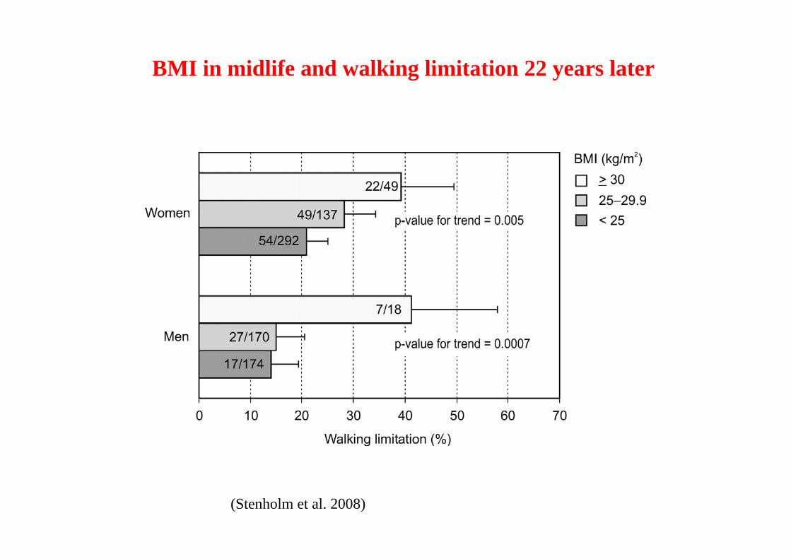
BMI in midlife and walking limitation 22 years later

(Stenholm et al. 2008)

A Additive genetic effectsC Shared environmental effectsE Individual environmental effects

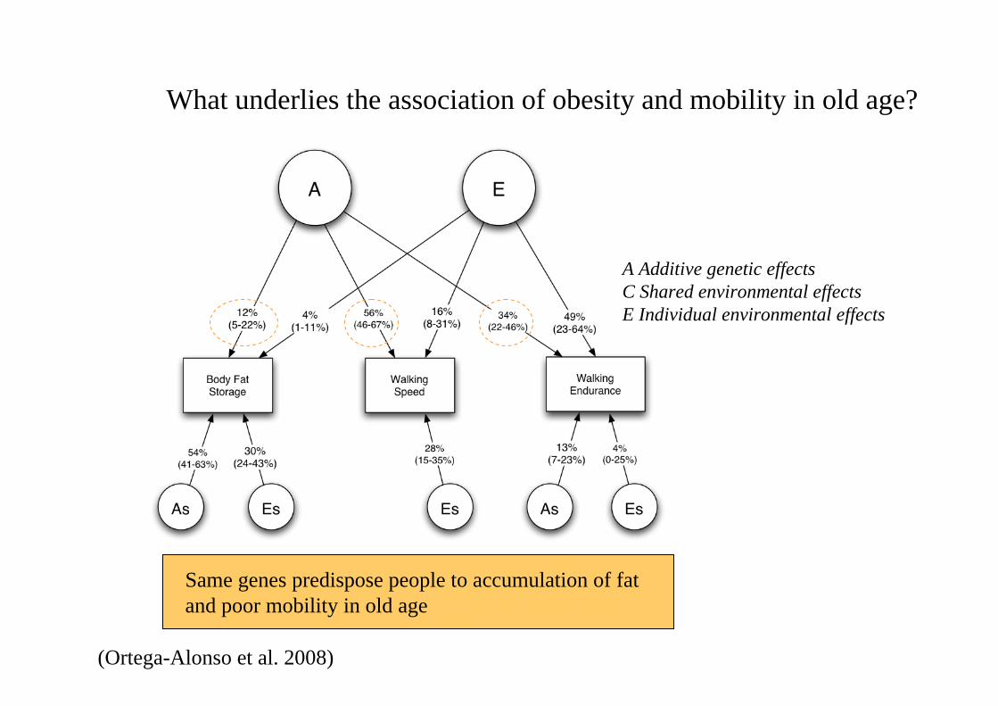
(Ortega-Alonso et al. 2008)

What underlies the association of obesity and mobility in old age?

Same genes predispose people to accumulation of fatand poor mobility in old age

Self-rated healthDisease severity Maximalwalking speed

Depressivesymptoms

A1D1 C2

E1 E2 E3 E4

0.34(0.07)

-0.55(0.02)

0.17(0.05)

-0.80(0.05)

-0.55(0.02)

-0.19(0.06)

0.70(0.06)

0.63(0.04)

0.98(0.03)

0.46(0.09)-0.09

(0.04)

-0.32(0.06)

0.63(0.04)

0.13(0.05)

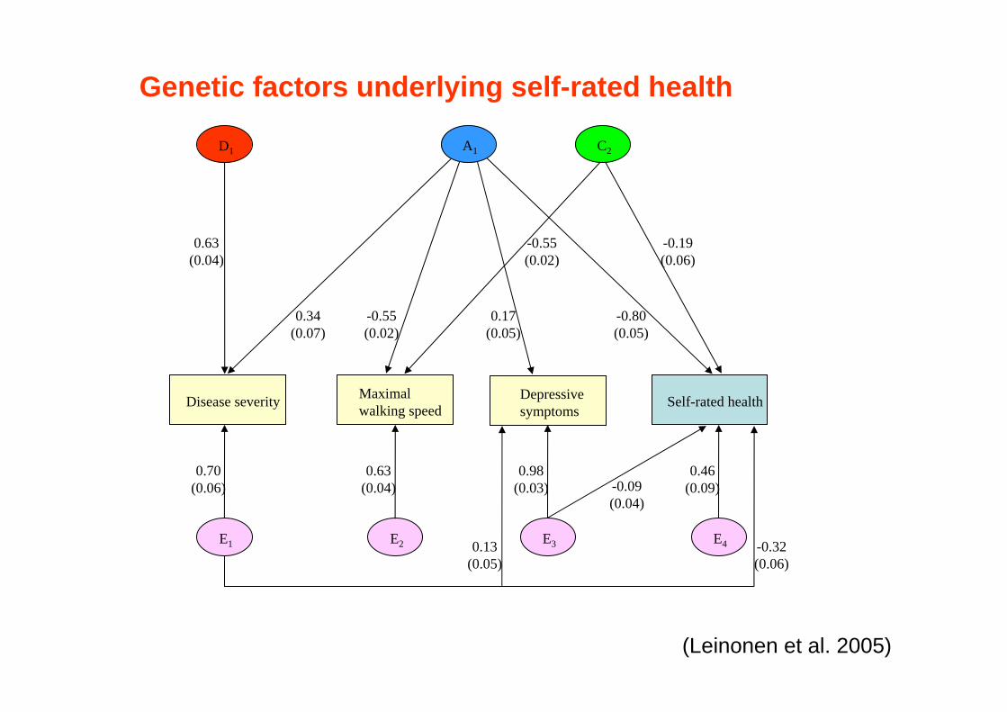
Genetic factors underlying self-rated health

(Leinonen et al. 2005)

Interpretation of the analysis among discordanttwins

Supporting a causal link between the risk factor and increased risk of outcome

IncreasedIncreasedIncreased

Specific genetic composition is associated with boththe risk factor and outcome

UnchangedIncreasedIncreased

Childhood environment and/or genetic factorsexplain the association between risk factor and outcome

UnchangedUnchangedIncreased

MZ pairsDZ pairs

Interpretation of resultPairwise analyses among twinpairs discordant for a specificrisk factor

Individual–basedanalyses

Ris

k•One twin has the exposure and other does not•Risk of exposed vs. not exposed

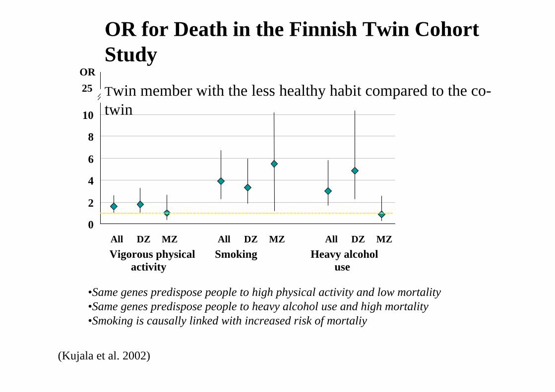
OR for Death in the Finnish Twin CohortStudyTwin member with the less healthy habit compared to the co-twin

Vigorous physical Smoking Heavy alcohol activity use

OR25

0

2

4

6

8

10

All DZ MZ All DZ MZ All DZ MZ

(Kujala et al. 2002)

•Same genes predispose people to high physical activity and low mortality•Same genes predispose people to heavy alcohol use and high mortality•Smoking is causally linked with increased risk of mortaliy

Esimerkki: KaksostutkimusGeneettisten tekijöiden kontrollointi

Diskordantit paritesim. toinen tupakoi ja toinen ei tupakoi

Mahdollistaa altistuksen ja päätepoisteen välisen yhteyden tutkimisen geneettisesti kontrolloidussapopulaatiossa

MZ – kaksoset 100% samat geenitDZ – kaksoset 50% samat geenit

• Goal: incease of healthy life expectancy• Means: prevention of disease, early detection

of diosease, treatment of disease, rehabilitation, social security and benefits

• Health policy is applying these in a meaningfull way

Health promotion

Individual vs. population• Effects of risk factors at the individual level?

• ”Truth” at population level, individual level ”truth”impossible to know

• E.g. stopping smoking may prevent coronary heartdisease and sudden death at the age of 55 but mayexpose the person to painfull death because of cancerten years later