Chapter 2 Basics of High-Voltage Test Techniques Abstract High-voltage (HV) testing utilizes the phenomena in electrical insula- tions under the influence of the electric field for the definition of test procedures and acceptance criteria. The phenomena—e.g., breakdown, conductivity, polari- zation and dielectric losses—depend on the insulating material, on the electric field generated by the test voltages and shaped by the electrodes as well as on envi- ronmental influences. Considering the phenomena, this chapter describes the common basics of HV test techniques, independent on the kind of the stressing test voltage. All details related to the different test voltages are considered in the relevant Chaps. 3–8. 2.1 External and Internal Insulations in the Electric Field In this section definitions of phenomena in electrical insulations are introduced. The insulations are classified for the purpose of high-voltage (HV) testing. Fur- thermore environmental influences to external insulation and their treatment for HV testing are explained. 2.1.1 Principles and Definitions When an electrical insulation is stressed in the electric field, ionization causes electrical discharges which may grow from one electrode of high potential to the one of low potential or vice versa. This may cause a high current rise, i.e., the dielectric looses its insulation property and thus its function to separate different potentials in an electric apparatus or equipment. For the purpose of this book, this phenomenon shall be called ‘‘breakdown’’ related to the stressing voltage: W. Hauschild and E. Lemke, High-Voltage Test and Measuring Techniques, DOI: 10.1007/978-3-642-45352-6_2, ȑ Springer-Verlag Berlin Heidelberg 2014 17
Transcript
Chapter 2Basics of High-Voltage Test Techniques
Abstract High-voltage (HV) testing utilizes the phenomena in electrical insula-tions under the influence of the electric field for the definition of test proceduresand acceptance criteria. The phenomena—e.g., breakdown, conductivity, polari-zation and dielectric losses—depend on the insulating material, on the electric fieldgenerated by the test voltages and shaped by the electrodes as well as on envi-ronmental influences. Considering the phenomena, this chapter describes thecommon basics of HV test techniques, independent on the kind of the stressing testvoltage. All details related to the different test voltages are considered in therelevant Chaps. 3–8.
2.1 External and Internal Insulations in the Electric Field
In this section definitions of phenomena in electrical insulations are introduced.The insulations are classified for the purpose of high-voltage (HV) testing. Fur-thermore environmental influences to external insulation and their treatment forHV testing are explained.
2.1.1 Principles and Definitions
When an electrical insulation is stressed in the electric field, ionization causeselectrical discharges which may grow from one electrode of high potential to theone of low potential or vice versa. This may cause a high current rise, i.e., thedielectric looses its insulation property and thus its function to separate differentpotentials in an electric apparatus or equipment. For the purpose of this book, thisphenomenon shall be called ‘‘breakdown’’ related to the stressing voltage:
W. Hauschild and E. Lemke, High-Voltage Test and Measuring Techniques,DOI: 10.1007/978-3-642-45352-6_2, � Springer-Verlag Berlin Heidelberg 2014
Definition The breakdown is the failure of insulation under electric stress, inwhich the discharge completely bridges the insulation under test and reduces thevoltage between electrodes to practically zero (collapse of voltage).
Note In IEC 60060-1 (2010) this phenomenon is referred to as ‘‘disruptive discharge’’.There are also other terms, like ‘‘flashover’’ when the breakdown is related to a dischargeover the surface of a dielectric in a gaseous or liquid dielectric, ‘‘puncture’’ when it occursthrough a solid dielectric and ‘‘sparkover’’ when it occurs in gaseous or liquid dielectrics.
In homogenous and slightly non-homogenous fields a breakdown occurs when acritical strength of the stressing field is reached. In strongly non-homogenousfields, a local stress concentration causes a localized electrical partial discharge(PD) without bridging the whole insulation and without breakdown of the stressingvoltage.
Definition A partial discharge is a localized electrical discharge that only partlybridges the insulation between electrodes, for details see Chap. 4.
Figure 1.2 shows the application of some important insulating materials. Tilltoday atmospheric air is applied as the most important dielectric of the externalinsulation of transmission lines and the equipment of outdoor substations.
Definition External insulation means air insulation including the outer surfaces ofsolid insulation of equipment exposed to the electric field, atmospheric conditions(air pressure, temperature, humidity) and to other environmental influences (rain,snow, ice, pollution, fire, radiation, vermin).
External insulation recovers its insulation behaviour in most cases after abreakdown and is then called a self-restoring insulation. In opposite to that, theinternal insulation of apparatus and equipment—such as transformers, gas-insu-lated switchgear (GIS), rotating machines or cables—is more affected by dis-charges, often even destroyed when a breakdown is caused by a HV stress.
Definition Internal insulation of solid, liquid or gaseous components is protectedfrom direct influences of external conditions such as pollution, humidity andvermin.
Solid and liquid- or gas-impregnated laminated insulation elements are non-self-restoring insulations. Some insulation is partly self-restoring, particularlywhen it consists e.g., of gaseous and solid elements. An example is the insulationof a GIS which uses SF6 gas and solid spacers. In case of a breakdown in an oil- orSF6 gas-filled tank, the insulation behaviour is not completely lost and recoverspartly. After a larger number of breakdowns, partly self-restoring elements have aremarkably reduced breakdown voltage and are not longer reliable.
The insulation characteristic has consequences for HV testing: Whereas for HVtesting of external insulation, the atmospheric and environmental influences haveto be taken into consideration, internal insulation does not require related specialtest conditions. In case of self-restoring insulation, breakdowns may occur duringHV tests. For partly self-restoring insulation, a breakdown would only be
acceptable in the self-restoring part of the insulation. In case of non-self restoringinsulation no breakdown can be accepted during a HV test. For the details see Sect.2.4 and the relevant subsections in Chaps. 3 and 6–8.
The test procedures should guarantee the accuracy and the reproducibility ofthe test results under the actual conditions of the HV test. The different testprocedures necessary for external and internal insulations should deliver compa-rable test results. This requires regard to various factors such as
• random nature of the breakdown process and the test results,• polarity dependence of the tested or measured characteristics,• acclimatisation of test object to the test conditions,• simulation of service conditions during the test,• correction of differences between standard, test and service conditions, and• possible deterioration of the test object by repetitive voltage applications.
2.1.2 HV Dry Tests on External Insulation IncludingAtmospheric Correction Factors
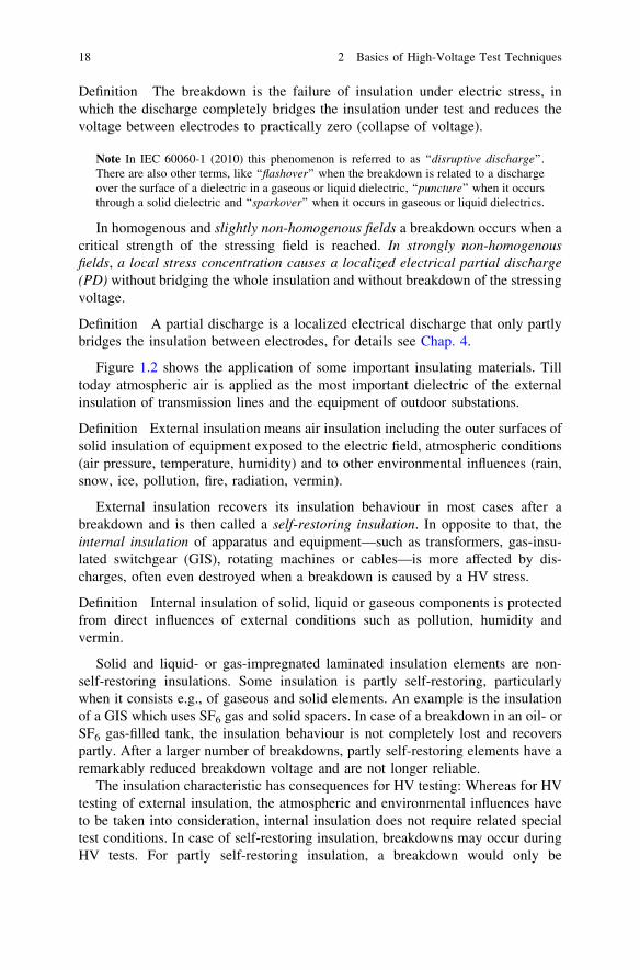
HV dry tests have to be applied for all external insulations. The arrangement of thetest object may affect the breakdown behaviour and consequently the test result.The electric field at the test object is influenced by proximity effects such asdistances to ground, walls or ceiling of the test room as well as to other earthed orenergized structures nearby. As a rule of thumb, the clearance to all externalstructures should be not less than 1.5 times the length of the possible dischargepath along the test object. For maximum AC and SI test voltages above 750 kV(peak), recommendations for the minimum clearances to external earthed orenergized structures are given in Fig. 2.1 (IEC 60060-1:2010). When the necessaryclearances are considered, the test object will not be affected by the surroundingstructures.
Atmospheric conditions may vary in wide ranges on the earth. Nevertheless, HVtransmission lines and equipment with external insulations have to work nearlyeverywhere. This means on one hand that the atmospheric service conditions forHV equipment must be specified (and for these conditions it must be tested), andon the other hand the test voltage values for insulation coordination (IEC 60071:2010) must be related to a standard reference atmosphere (IEC 60060-1:2010):
The temperature shall be measured with an expanded uncertainty t B 1 �C, theambient pressure with p B 2 hPa. The absolute humidityh can be directly mea-sured with so-called ventilated dry-and wet-bulb thermometers or determined fromthe relative humidityR and the temperature t by the formula (IEC 60060-1:2010):
2.1 External and Internal Insulations in the Electric Field 19
If HV equipment for a certain altitude shall be designed according to thepressure-corrected test voltages, the relationship between altitude H/m andpressure p/hPa is given by
p ¼ 1; 013 � e H8150: ð2:2Þ
A test voltage correction for air pressure based on this formula can be rec-ommended for altitudes up to 3,000 m. For more details see Pigini et al. (1985),Ramirez et al. (1987) and Sun et al. (2009). The temperature t and the pressure pdetermine the air densityd, which influences the breakdown process directly:
d ¼ p
p0� 273þ t0
273þ t: ð2:3Þ
The air density delivers together with the air density correction exponent m(Table 2.1) the air density correction factor
k1 ¼ dm: ð2:4Þ
The humidity affects the breakdown process especially when it is determined bypartial discharges. These are influenced by the kind of test voltage. Therefore, fordifferent test voltages different humidity correction factors k2 have to be applied,which are calculated with the parameter k and the humidity correction exponent w
k2 ¼ kw; ð2:5Þ
0
peak of test voltage V p
16
m
12
8
4
clearance
400 800 1200 1600 kV 2000
Fig. 2.1 Recommendedclearances between testobject and extraneousenergized or earthedstructures
20 2 Basics of High-Voltage Test Techniques
with
DC : k ¼ 1þ 0:014 h=d� 11ð Þ � 0:00022 h=d� 11ð Þ2 for 1 g=m3\h=d;\15 g=m3;AC : k ¼ 1þ 0:012 h=d� 11ð Þ for 1 g=m3\h=d\15 g=m3;LI/SI : k ¼ 1þ 0:010 h=d� 11ð Þ for 1 g=m3\h=d\20 g=m3:
The correction exponents m and w describe the characteristic of possible partialdischarges and are calculated utilizing a parameter
g ¼ V50
500 � L � d � k ; ð2:6Þ
withV50 Measured or estimated 50 % breakdown voltage at the actual atmospheric
conditions, in kV (peak),L Minimum discharge path, in m,d Relative air density andk Dimension-less parameter defined with formula (2.5).
Note For withstand tests it can be assumed V50 � 1:1 � Vt (test voltage). Depending on theparameter g (Eq. 2.6), Table 2.1 or Fig. 2.2 delivers the exponents m and w.
According to IEC 60060-1:2010 the atmospheric correction factor
Kt ¼ k1 � k2; ð2:7Þ
shall be used to correct a measured breakdown voltage V to a value under standardreference atmosphere
V0 ¼ V=Kt: ð2:8Þ
Vice versa when a test voltage V0 is specified for standard reference atmo-sphere, the actual test voltage value can be calculated by the converse procedure:
V ¼ Kt � V0: ð2:9Þ
Because the converse procedure uses the breakdown voltage V50 (Eq. 2.6), theapplicability of Eq. (2.9) is limited to values of Kt close to unity, for Kt \ 0.95 it is
Table 2.1 Air density andhumidity correctionexponents m and w accordingto IEC 60060-1:2010
2.1 External and Internal Insulations in the Electric Field 21
recommended to apply an iterative procedure which is described in detail in AnnexE of IEC 60060-1:2010.
It is necessary to mention that the present procedures for atmospheric correc-tions are not yet perfect (Wu et al. 2009). Especially the humidity correction islimited only to air gaps and not applicable to flashovers directly along insulatingsurfaces in air. The reason is the different absorption of water by different surfacematerials. Furthermore the attention is drawn to the limitations of the applicationof humidity correction to h/d B 15 g/m3 (for AC and DC test voltages), respec-tively h/d B 20 g/m3 (for LI and SI test voltages). The clarification of the humiditycorrection for surfaces as well as the extension of their ranges requires furtherresearch work (Mikropolulos et al. 2008; Lazarides and Mikropoulos 2010; 2011)as well as the atmospheric correction in general for altitudes above 2,500 m
0 0.5 1.0 1.5 2.0
parameter g
1.0
0.8
0.6
0.4
0.2
exponent m
0 0.5 1.0 1.5 2.0 2.5 3.0
parameter g
1.0
0.8
0.6
0.4
0.2
exponent w
3.02.5
(a)
(b)
Fig. 2.2 Correctionexponents according to IEC60060-1:2010. am for airdensity. bw for air humidity
22 2 Basics of High-Voltage Test Techniques
(Ortega and Waters et al. 2007; Jiang et al. 2008; Jiang and Shu et al. 2008).Nevertheless, also the available correction to and from reference atmosphericconditions is important in HV testing of external insulation as it should be shownby two simple examples.
Example 1 In a development test, the 50 % LI breakdown voltage of an air insulateddisconnector [breakdown (flashover) path L = 1 m, not at the insulator surface] wasdetermined to V50 = 580 kV at a temperature of t = 30 �C, an air pressure ofp = 980 hPa and a humidity of h = 12 g/m3. The value under reference atmosphericconditions shall be calculated:
Air density d = (995/1,013) � (293/303) = 0.95;Parameter k = 1 ? 0.010 � ((12/0.95) -
11) = 1.02;Parameter g = 580/(500 � 1 � 0.95 � 1.02) = 1.20;Table 2.1: delivers the air density correctionexponent
m = 1.0;
and the humidity correction exponent w = (2.2 - 1.2) (2.0 - 1.2)/0.8 = 1.0;With the density correction factor k1 = 0.95;and the humidity correction factor k2 = 1.02;one gets the atmospheric correction factor Kt = 0.95 � 1.02 = 0.97.Under reference conditions the 50 % breakdownvoltage would be
V0250 = 580/0.97 = 598 kV.
Example 2 The same disconnector shall be type tested with a LI voltage of V0 = 550 kVin a HV laboratory at higher altitude under the conditions t = 15 �C, p = 950 hPa andh = 10 g/m3. Which test voltage must be applied?
Air density d = (950/1013) (293/288) = 0.954;parameter k = 1 ? 0.010 ((10/0.95) -
11) = 0.995;parameter g = 598/(500 � 1 � 0.95 � 0.995) = 1.265;Table 2.1: delivers the air density correctionexponent
m = 1.0;
and the humidity correction exponent w = (2.2 - 1.265)(2.0 - 1.265)/0.8 = 0.86;
With the density correction factor k1 = 0.954;and the humidity correction factor k2 = 0.9950.86 = 0.996;one gets the atmospheric correction factor Kt = 0.954 � 0.996 = 0.95.Under the actual laboratory conditions the testvoltage is
V = 550 � 0.95 = 523 kV.
The two examples show, that the differences between the starting and resultingvalues are significant. The application of atmospheric corrections is essential forHV testing of external insulation.
2.1 External and Internal Insulations in the Electric Field 23
2.1.3 HV Artificial Rain Tests on External Insulation
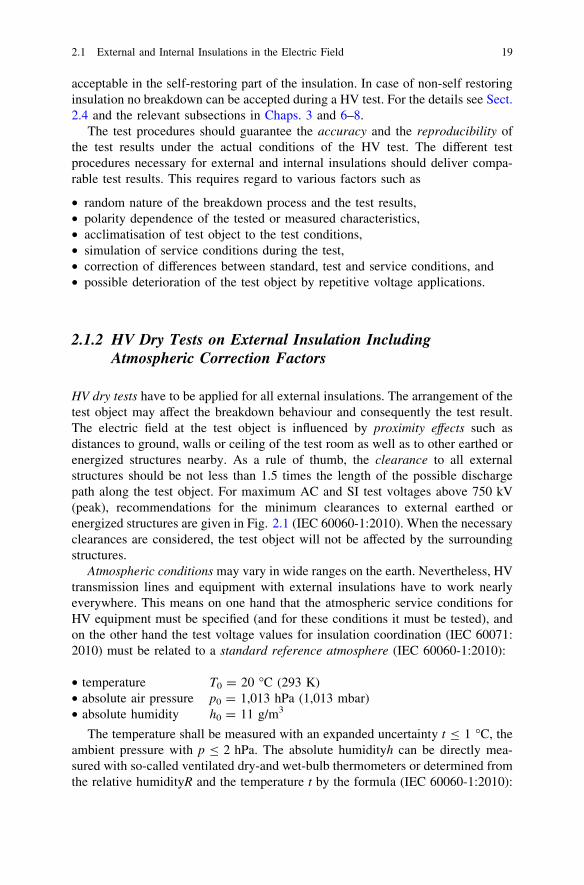
External HV insulations (especially outdoor insulators) are exposed to natural rain.The effect of rain to the flashover characteristic is simulated in artificial rain (orwet) tests (Fig. 2.3). The artificial rain procedure described in the following isapplicable for tests with AC, DC and SI voltages, whereas the arrangement of thetest object is described in the relevant apparatus standards.
The test object is sprayed with droplets of water of given resistivity and tem-perature (Table 2.2). The rain shall fall on the test object under an angel of about45�, this means that the horizontal and vertical components of the precipitationrate shall be identical. The precipitation rate is measured with a special collectingvessel with a horizontal and a vertical opening of identical areas between 100 and700 cm2. The rain is generated by an artificial rain equipment consisting of nozzlesfixed on frames. Any type of nozzles which generates the appropriate rain con-ditions (Table 2.2) can be applied.
Note 1 Examples of applicable nozzles are given in the old version of IEC 60-1:1989-11(Fig. 2, pp. 113–115) as well as in IEEE Std. 4–1995.
The precipitation rate is controlled by the water pressure and must be adjustedin such a way, that only droplets are generated and the generation of water jets orfog is avoided. This becomes more and more difficult with increasing size of thetest objects which requires larger distances between test object and artificial rainequipment. Therefore, the requirements of IEC 60060-1:2010 are only related toequipment up to rated voltages of Vm = 800 kV, Table 2.2 contains an actualproposal for the UHV range.
The reproducibility of wet test results (wet flashover voltages) is less than thatfor dry HV breakdown or withstand tests. The following precautions enableacceptable wet test results:
• The water temperature and resistivity shall be measured on a sample collectedimmediately before the water reaches the test object.
• The test object shall be pre-wetted initially for at least 15 min under the con-ditions specified in Table 2.2 and these conditions shall remain within thespecified tolerances throughout the test, which should be performed withoutinterrupting the wetting.
Note 2 The pre-wetting time shall not include the time needed for adjusting the spray. It isalso possible to perform an initial pre-wetting by unconditioned tap water for 15 min,followed without interruption of the spray by a second pre-wetting with the well condi-tioned test water for at least 2 min before the test begins.
• The test object shall be divided in several zones, where the precipitation rate ismeasured by a collecting vessel placed close to the test object and moved slowlyover a sufficient area to average the measured precipitation rate.
24 2 Basics of High-Voltage Test Techniques
• Individual measurements shall be made at all measuring zones considering alsoone at the top and one near the bottom of the test object. A measuring zone shallhave a width equal to that of the test object (respectively its wetted parts) and a
single line of nozzlesFig. 2.3 Artificial rain teston an 800 kV supportinsulator (Courtesy HSPCologne)
Table 2.2 Conditions for artificial rain precipitation
Precipitation condition Unit IEC 60060-1:2010 rangeforequipment of Vm B 800 kV
Proposed range for UHVequipment Vm [ 800 kV
Average precipitationrate of allmeasurements:
• Vertical component (mm/min) 1.0–2.0 1.0–3.0• Horizontal component (mm/min) 1.0–2.0 1.0–3.0Limits for any individual
measurement and foreach component
(mm/min) ±0.5 from average 1.0–3.0
Temperature of water (�C) Ambient temperature±15 K
Ambient temperature±15 K
Conductivity of water (lS/cm) 100 ± 15 100 ± 15
2.1 External and Internal Insulations in the Electric Field 25
maximum height of 1–2 m. The number of measuring zones shall cover the fullheight of the test object.
• The spread of results may be reduced if the test object is cleaned with a surface-active detergent, which has to be removed before the beginning of wetting.
• The spread of results may also be affected by local anomalous (high or low)precipitation rates. It is recommended to detect these by localized measurementsand to improve the uniformity of the spray, if necessary.
The test voltage cycle for an artificial rain test shall be identical to that for a drytest. For special applications different cycles are specified by the relevant appa-ratus committees. A density correction factor according to Sect. 2.1.2, but nohumidity correction shall be applied.
Note 3 IEC 60060-1:2010 permits one flashover in AC and DC wet tests provided that in arepeated test no further flashover occurs.
Note 4 For the UHV test voltage range, it may be necessary to control the electric field(e.g., by toroid electrodes) to the artificial rain equipment and/or to surrounding groundedor energized objects including walls and ceiling to avoid a breakdown to them. Alsoartificial rain equipment on a potential different from ground might be taken intoconsideration.
2.1.4 HV Artificial Pollution Tests on External Insulation
Outdoor insulators are not only exposed to rain, but also to pollution caused bysalt fog near the sea shore, by industry and traffic or simply by natural dust.Depending on the position of a transmission line or substation, the surrounding isclassified in several different pollution classes between low (surface conductivityjs B 10 lS) and extreme (js C 50 lS) (Mosch et al. 1988). The severity of thepollution class can also be characterized by the equivalent salinity (SES in kg/m3),which is the salinity [content of salt (in kg) in tap water (in m3)] applied in a salt-fog test according to IEC 60507 (1991) that would give comparable values of theleakage current on an insulator as produced at the same voltage by natural pol-lution on site (Pigini 2010).
Depending on the pollution class, the artificial pollution test is performed withdifferent intensities of pollution, because the test conditions shall be representativeof wet pollution in service. This does not necessarily mean that any real servicecondition has to be simulated. In the following the performance of typical pol-lution tests is described without considering the representation of the pollutionzones. The pollution flashover is connected with quite high pre-arc currents sup-plied via the wet and polluted surface from the necessary powerful HV generator(HVG). In a pioneering work, Obenaus (1958) considered a flashover model of aseries connection of the pre-arc discharge with a resistance for the polluted sur-face. Till today the Obenaus model is the basis for the selection of pollution testprocedures and the understanding of the requirements on test generators(Slama et al. 2010; Zhang et al. 2010). These requirements to HV test circuits are
26 2 Basics of High-Voltage Test Techniques
considered in the relevant Chaps. 3 and 6–8. Pollution tests of insulators for highaltitudes have to take into consideration not only the pollution class, but also theatmospheric conditions (Jiang et al. 2009).
The test object (insulator) must be cleaned by washing with tap water and thenthe pollution process may start. Typically the pollution test is performed withsubsequent applications of the test voltage which is held constant for a specified testtime of at least several minutes. Within that time very heavy partial discharges, so-called pre-arcs, appear (Fig. 2.4). It may happen that the wet and polluted surfacedries (which means electrically withstand of the tested insulator and passing thetest) or that the pre-arcs are extended to a full flashover (which means failingthe test). Because of the random process of the pollution flashover, remarkabledispersion of the test results can be expected. Consequently the test must berepeated several times to get average values of sufficient confidence or to estimatedistribution functions (see Sect. 2.4). Two pollution procedures shall be described:
The salt-fog method uses a fog from a salt (NaCl) solution in tap water withdefined concentrations between 2.5 and 20 kg/m3 depending on the pollution zone.A spraying equipment generates a number of fog jets each generated by a pair of
Pre-arc appears at the stalk of the insulator (location of highest current density)
Pre-arc extends and bridges the distance between two sheds.
Further extension of the pre-arc leads to bridging of two sheds.
Further extension and combination of pre-arcs causes the flashover of the insulator (final arc).
Fig. 2.4 Phases of apollution flashover of aninsulator (Courtesy of FHZittau, Germany)
2.1 External and Internal Insulations in the Electric Field 27
nozzles. One nozzle supplies about 0.5 l/min of the salt solution, the other one thecompressed air with a pressure of about 700 kPa which directs the fog jet to thetest object. The spraying equipment contains usually two rows of the describeddouble nozzles. The test object is wetted before the test. The test starts with theapplication of the fog and the test voltage value which should be reached—but notovertaken—as fast as possible. The whole test may last up to 1 h.
The pre-deposit method is based on coating the test object with a conductivesuspension of Kieselgur or Kaolin or Tonoko in water (&40 g/l). The conductivityof the suspension is adjusted by salt (NaCl). The coating of the test object is madeby dipping, spraying or flow-coating. Then it is dried and should become inthermal equilibrium with the ambient conditions in the pollution chamber. Finallythe test object is wetted by a steam-fog equipment (steam temperature B 40 �C).The surface condition is described by the surface conductivity (lS) measured fromthe current at two probes on the surface (IEC 60-1:1989, Annex B.3) or by theequivalent amount of salt per square centimetre of the insulating surface [so-calledsalt deposit density (S.D.D.) in mg/cm2]. The test can start with voltage applicationbefore the test object is wetted, or after wetting, when the conductivity has reachedits maximum. Details depend on the aim of the test, see IEC 60507:1991.
Both described procedures can be performed with different aim of the pollutiontest:
• determination of the withstand voltage for a certain insulator of specified degreeof pollution and a specified test time,
• determination of the maximum degree of pollution for a certain insulator at aspecified test voltage and specified test time.
Pollution tests require separate pollution chambers, usually with bushings forthe connection of the test voltage generator. Because of the salt fog and humidity,the HV test system itself is outside under clean conditions. Inside a salt-fogchamber, the clearances around the test object should be C0.5 m/100 kV but notless than 2 m. When no pollution chamber is available, also tents from plastic foilmay be applied, to separate the pollution area from the other areas of a HVlaboratory.
2.1.5 HV Tests on Internal Insulation
In a HV test field, the HV components of test systems are designed with anexternal indoor insulation usually. When internal insulation shall be tested, the testvoltage must be connected to the internal part of the apparatus to be tested. This isusually done by bushings which have an external insulation. For reasons of theinsulation co-ordination or of the atmospheric corrections, cases will arise that theHV withstand test level of the internal insulation exceeds that of the externalinsulation (bushing). Then the withstand level of the bushing must be enhanced topermit application of the required test voltages for the internal insulation. Usually
28 2 Basics of High-Voltage Test Techniques
special ‘‘test bushings’’ of higher withstand level, which replace the ‘‘servicebushings’’ during the test, are applied. A further possibility is the immersion of theexternal insulation in liquids or compressed gases (e.g., SF6) during the test.
In rare cases, when the test voltage level of the external insulation exceeds thatof the internal insulation a test at the complete apparatus can only be performedwhen the internal insulation is designed according to the withstand levels of theexternal insulation. If this cannot be done, then the apparatus should be tested atthe internal test voltage level, and the external insulation should be tested sepa-rately using a dummy.
Internal insulation is influenced by the ambient temperature of the test field, butusually not by pressure or humidity of the ambient air. Therefore, the onlyrequirement is the temperature equilibrium of the test object with its surroundingwhen the HV test starts.
2.1.6 Hints to Further Environmental Tests and HV Testsof Apparatus
There are also other environmental HV tests, e.g., under ice or snow. They aremade with natural conditions in suitable open-air HV laboratories or in specialclimatic chambers (Sklenicka et al. 1999). Other environmental influences whichare simulated in HV tests are UV light (Kindersberger 1997), sandstorms (Fan andLi 2008) and fire under transmission lines. The HV test procedures for apparatusand equipment are described in the relevant ‘‘vertical’’ standards, examples aregiven in the chapters of the different test voltages.
2.2 HV Test Systems and Their Components
This section supplies a general description of HV test systems and their compo-nents, which consist of the HV generator, the power supply unit, the HVvoltagemeasuring system, the control system and possibly additional measuring equip-ment, e.g., for PD or dielectric measurement. In all cases the test object cannot beneglected, because it is a part of the HV test circuit.
A HV test system means the complete set of apparatus and devices necessary forperforming a HV test. It consists of the following devices (Fig. 2.5).
The HV generator (HVG) converts the supplied low or medium voltage into thehigh test voltage. The type of the generator determines the kind of the test voltage.For the generation of high alternating test voltages (HVAC), the HVG is a testtransformer (Fig. 2.6a). It might be also a resonance reactor which requires acapacitive test object (TO) to establish an oscillating circuit for the HVAC generation(see Sect. 3.1). For the generation of high direct test voltages (HVDC) the HVG is aspecial circuit of rectifiers and capacitors (e.g., a Greinacher or Cockroft-Walton
2.1 External and Internal Insulations in the Electric Field 29
generator, Fig. 2.6b, see Sect. 6.1), and for the generation of high lightning orswitching impulse (LI, SI) voltages, it is a special circuit of capacitors, resistors andswitches (sphere gaps) (e.g., a Marx generator, Fig. 2.6c, see Sect. 7.1).
The test object does not only play a role for HVAC generation by resonantcircuits, there is an interaction between the generator and the test object in all HVtest circuits. The voltage at the test object may be different from that at thegenerator because of a voltage drop at the HV lead between generator and testobject or even a voltage increase because of resonance effects. This means thevoltage must be measured directly at the test object and not at the generator(Fig. 2.5). For this voltage measurement a sub-system—usually called HVmeasuring system—is connected to the test object (Fig. 2.7a, see Sect. 2.3). Fur-ther sub-systems, e.g., for dielectric measurement, can be added. Up to few 10 kVsuch systems can be designed as compact units including voltage source(Fig. 2.7b). Very often PD measurements are performed during a HVAC test. Forthat a PD measuring system is connected to the AC test system (Fig. 2.7c). Allthese systems consist of a HV component (e.g., voltage divider, coupling orstandard capacitor), measuring cable for data transfer and a low-voltage instrument(e.g., digital recorder, peak voltmeter, PD measuring instrument, tan delta bridge).
All the components of a HV test system and the test object described aboveform the HV circuit. This circuit should be of lowest possible impedance. Thismeans, it should be as compact as possible. All connections, the HV leads and theground connections should be straight, short and of low inductance, e.g., by copperfoil (width 10–25 cm, thickness depending of current). In HV circuits used also forPD measurement, the HV lead should be realized by PD-free tubes of a diameterappropriate to the maximum test voltage. Any loop in the ground connection has tobe avoided.
Internet; LAN computer control digital recorder PD instrument
control & measuring system
high-voltage circuit
power supply generator test object voltage divider coupling capacitorregulator
Fig. 2.6 HV generators. a For AC test voltage 1,000 kV at Cottbus Technical University. b ForDC test voltage 1,500 kV at HSP Cologne. c For LI/SI test voltages 2,400 kV at DresdenTechnical University
The necessary power for the HV tests is supplied from the power grid—in caseof on-site testing also from a Diesel-generator set—via the power supply unit(Fig. 2.5). This unit consists of one or several switching cubicles and a regulationunit (regulator transformer or motor-generator set or thyristor controller orfrequency converter). It controls the power according to the signals from thecontrol system in such a way, that the test voltage at the test object is adjusted asrequired for the HV test. For safety reasons the switching cubicle shall have twocircuit breakers in series; the first switches the connections between the grid andthe power supply unit (power switch), the second one that between the powersupply unit and the generator (operation switch). For the reduction of the requiredpower from the grid in case of capacitive test objects, the power supply unit isoften completed by a fixed or even adjustable compensation reactor.
When the generator is the heart of HV test system then the control and mea-suring sub-system—usually called control and measuring system (Fig. 2.8;Baronick 2003)—is its brain. Older controls were separated from the measuringsystems and the adjustment of the test voltage was manually made by the operator(The brain was that of the operator). As a next step, programmable logic con-trollers have been introduced. Now a state-of-the-art control system is a computercontrol which enables the pre-selection of the test procedure with all test voltagevalues, gives the commands to the power supply unit, overtakes the data from themeasuring systems, performs the test data evaluation and prints a test record. Inthat way one operator can supervise very complex test processes. The test data canbe transferred to a local computer network (LAN) e.g., for combining with testdata from other laboratories or even to the Internet. The latter can also be used incase of technical problems for remote service.
2.2 HV Test Systems and Their Components 31
A HV test system is only complete when it is connected to a safety systemwhich protects the operators and the participants of a HV test. Among others, thesafety system includes a fence around the test area which is combined with theelectrical safety loop. The test can only be operated when the loop is closed, fordetails see Sect. 9.2.
HV divider
LV instrument
computer
HV connection cable
HV resonant test facility
controlunit
cable termination under test
couplingcapacitor
measuringimpedance
calibratorcomputerized PD measuring system
voltage divider (compressed gas capacitor)
HV test transformer
(a)
(c)
(b)
Fig. 2.7 Measuring systems. a Voltage measuring system with digital recorder includingimpulse generator. b Compact capacitance/loss factor measuring system with integrated ACvoltage source (Courtesy of Doble-Lemke). c Partial discharge measuring system including ACvoltage test circuit (Courtesy of Doble-Lemke)
2.3 HV Measurement and Estimation of the MeasuringUncertainty
This section is related to voltage measurement and describes HV measuring systems,their calibration and the estimation of their uncertainties of measurements. Precisemeasurement of high test voltages is considered to be a difficult task for many years(Jouaire and Sabot et al. 1978; ‘‘Les Renardieres Group’’ 1974). This situation isalso reflected by the older editions of the relevant standard IEC 60060-2. For goodpractice in HV test fields, this Sect. 2.3 on HV measurement and uncertainty esti-mation is closely related to the newest edition of the standard IEC 60060-2:2010.
The terms ‘‘uncertainty’’, ‘‘error’’ and ‘‘tolerance’’ are often mixed up.Therefore, the following clarification seems needed: The uncertainty is a param-eter which is associated with the result of a measurement. It characterizes thedispersion of the results due to the characteristics of the measuring system. Theerror is the measured quantity minus a reference value for this quantity and thetolerance is the permitted difference between the measured and the specified value.Tolerances play a role for standard HV test procedures (Sects. 3.6, 6.5 and 7.6).Uncertainties are important for the decision, whether a measuring system isapplicable or not for acceptance testing.
2.3.1 HV Measuring Systems and Their Components
Definition: A HV measuring system(MS) is a ‘‘complete set of devices suitablefor performing a HV measurement’’. Software for the calculation of the result ofthe measurement is a part of the measuring system (IEC 60060-2:2010).
PD V
Switching cubicle
PLC IPC for control
and measurement
service center
separate test system
management
router
router
optic Ethernet (system LAN)
optic Profibus
user LAN
INTERNET
Fig. 2.8 Computerized control and measuring system
2.3 HV Measurement and Estimation of the Measuring Uncertainty 33
A HV measuring system (Fig. 2.9) which should be connected directly to the testobject consists usually of the following components
• A converting device including its HV and earth connection to the test objectwhich converts the quantity to be measured (measurand: test voltage with itsvoltage and/or time parameters) into a quantity compatible with the measuringinstrument (low-voltage or current signal). It is very often a voltage divider of atype depending on the voltage to be measured (Fig. 2.10). For special applicationalso a voltage transformer, a voltage converting impedance (carrying a mea-surable current) or an electric field probe (converting amplitude and timeparameters of an electric field) may be used. The clearances between the con-verting device and nearby earthed or energized structures may influence theresult of the measurement. Such proximity effects shall be considered by theuncertainty estimation (see Sect. 2.3.4). To keep the contribution of the proximityeffect to the uncertainty of measurement small, the clearances of movable con-verting devices should be as those recommended for the test object (seeSect. 2.1.2 and Fig. 2.1). If the converting device is always in a fixed position andthe measuring system is calibrated on site, the proximity effect can be neglected.
• A transmission system which connects the output terminals of the convertingdevice with the input terminals of the measuring instrument. It is very often acoaxial cable with its terminating impedance, but may also be an optical link whichincludes a transmitter, an optical cable and a receiver with an amplifier. For specialapplication also cable connections with amplifiers and/or attenuators are in use.
Fig. 2.9 HV measuringsystem consisting of voltagedivider, coaxial cable andPC-based digital recorder
34 2 Basics of High-Voltage Test Techniques
• A measuring instrument suitable to measure the required test voltage parametersfrom the output signal of the transmission system. Measuring instruments forHV application are usually special devices which fulfil the requirements of theIEC Standards 61083 (part 1 and 2 for LI/SI test voltages has been published,part 3 and 4 for AC/DC voltages is under preparation). The conventional ana-logue peak voltmeters are replaced by digital peak voltmeters and more andmore by digital recorders (Fig. 2.11). Digital recorders measure both test volt-age and time parameters. This is mandatory for LI/SI test voltages, but more andmore also for AC/DC test voltages with respect to changes in time by voltage
high-resistive divider for DC
low-resistive divider for LI
capacitive divider for AC and SI
damped capacitive divider for LI,SI,(AC)
universal divider for all voltages
Fig. 2.10 Kinds and applications of voltage dividers
stand-alone device marked components built into a control desk(a) (b)
Fig. 2.11 Instruments for HV measurement. a Digital AC/DC peak voltmeter. b LI/SI digitalrecorder
2.3 HV Measurement and Estimation of the Measuring Uncertainty 35
drop (see Sects. 3.2.1 and 6.2.3.2), harmonics (AC, see Sect. 3.2.1) or ripple(DC, see Sect. 6.2.1).
Each HV measuring system is characterized by its operating conditions, as theyare the rated operating voltage, the measurement ranges, the operating time(or kind and number of LI/SI voltage applications) and the environmental con-ditions. The dynamic behaviour of a measuring system can be described as anoutput signal depending on frequency (frequency response for AC and DC voltagemeasuring systems, Fig. 2.12a) or on a voltage step (step response for LI/SIvoltage measuring systems, Fig. 2.12b) or by a sufficiently low uncertainty of LI/SI parameter measurement within the nominal epoch of the measuring system.
Note The nominal epoch of an impulse voltage, which will be explained more in detail inSects. 7.2 and 7.3, is the range between the minimum and the maximum of the relevant LI/SI time parameter for which the measuring system is approved. The nominal epoch is
+3 dB
0
-3 dB
f1A f2A 2B
frequency to be measured
normalized deviation of output amplitude
output signal normalized on steady state
1
00.03 0.1 0.3 0.5 1 3 μs
example:nominal epoch of LI/LIC
settling time
±2%deviation
virtual origin
A
B
100.05
f
(a)
(b)
Fig. 2.12 Response ofmeasuring systems (IEC60060-2:2010). a Frequencyresponse (curve A with lowerand upper limit frequency,curve B with upper frequencylimit, related to AC/DCmeasurement). b Unit stepresponse after a step-voltageinput (related to LI/SI voltagemeasurement, see Sect. 7.3)
derived from the upper and lower tolerances of the front time parameter of the impulsevoltage.
All these rated values have to be supplied by the manufacturer of the measuringsystem (respectively its components) after type and routine tests. They should fit tothe requirements and the conditions of the HV test field where the measuringsystem shall be applied.
Furthermore each voltage measuring system is characterized by its scale factor,this means the value by which the reading of the instrument must be multiplied toobtain the input quantity of the HV measuring system (voltage and time param-eters). For measuring systems that display the value of the input quantity directly,the scale factor is unity. In that case—and transmission by a coaxial cable—thescale factor of the instrument is the inverse of the scale factor of the convertingdevice. A correctly terminated coaxial cable has the scale factor unity, other typesof transmission systems may have one different from unity.
The scale factor must be calibrated to guarantee a voltage measurementtraceable to the National Standard of measurement. The calibration consists of twomain parts. On one hand the value of the scale factor shall be determined includingthe necessary dynamic behaviour. On the other hand, the uncertainty of the HVmeasurement shall be estimated. When the uncertainty and the dynamic behaviourare within the limits given by IEC 60060-2:2010, the approved measuring system(AMS) is applicable for measurement in an accredited HV test field (see therelevant Chaps. 3, 6 and 7).
2.3.2 Approval of a HV Measuring System for an AccreditedHV Test Field
A HV measuring system is qualified for the use in an accredited HV test field byseveral successful tests and checks described in IEC 60060-2:2010. It becomes an‘‘AMS’’ when it has passed the following tests and checks:
• The type test by the manufacturer on the system or its components on sample(s)from the production shall demonstrate the correct design and conformity withthe requirements. These requirements include the determination of
– the scale factor value, its linearity and its dynamic behaviour,– its short and long term stability,– the ambient temperature effect, i.e., the influence of the ambient temperature,– the proximity effect, i.e., the influence of nearby grounded or energized
structures,– the software effect i.e., the influence of software on the dispersion of
measurements,– the demonstration of withstand in a HV test.
2.3 HV Measurement and Estimation of the Measuring Uncertainty 37
• The routine test on each system or each of its components by the manufacturershall demonstrate the correct production and the conformity with the require-ments by
– the scale factor value, its linearity and its dynamic behaviour and also– the demonstration of withstand in a HV test.• The performance test on the ‘‘complete measuring system’’ shall characterize it
at its place in the HV test field ‘‘under operation conditions’’ by determination of
– the scale factor value, its linearity and its dynamic behaviour;– the long term stability (from repetitions of performance tests) and– the proximity effects.
The user is responsible for the performance tests and should repeat them annually,but at least once in 5 years (IEC 60060-2:2010).• The performance check is a ‘‘simple procedure’’—usually the comparison with a
second AMS or with a standard air gap (see Sect. 2.3.5)—‘‘to ensure thatthe most recent performance test is still valid’’. The user is responsible for theperformance checks and should repeat them according to the stability of theAMS, but at least annually (IEC 60060-2:2010).
The mentioned single tests are described together with the uncertainty esti-mation in Sect. 2.3.4. For the reliable operation of the measuring system a HVwithstand test of the converting device is necessary as a type test and, if theclearances in the laboratory of use are limited, also in a first performance test. Theusually required withstand test voltage level is 110 % of the rated operatingvoltage of the converting device. The test procedure shall follow those typical forthe relevant test voltages (Sects. 3.6, 6.5 and 7.6). In case of a converting devicefor outdoor application, the type test should include an artificial rain test.
This first performance test shall also include an interference test of the trans-mission system (coaxial cable) and the instrument of LI/SI measuring systemsdisconnected from the generator, but in their position for operation. This testgenerates an interference condition at the short-circuited input of the transmissionsystem by firing the related impulse voltage generator at a test voltage represen-tative for the highest operating voltage of the measuring system. The interferencetest is successful, when the measured amplitude of the interference is less than 1 %of the test voltage to be measured.
The results of all tests and checks shall be reported in the ‘‘record of perfor-mance’’ of the measuring system, which shall be established and maintained by theuser of the AMS (IEC 60060-2:2010). This record shall also contain a detailedtechnical description of the AMS. It is the right of an inspector of an acceptancetest of any apparatus to see the record of performance for the used HV measuringsystem.
As required in performance tests, the scale factor, the linearity and the dynamicbehaviour of a complete measuring system can be determined by different meth-ods. The most important and preferred method is the comparison with a reference
measuring system (RMS), in the following called ‘‘comparison method’’ (IEC60060-2:2010) and described in the following subsection.
Note An alternative is the ‘‘component method’’ which means the determination of thescale factor of the measuring system from the scale factors of its components (IEC 60060-2:2010). The scale factor of the components can be determined by the comparison with areference component of lower uncertainty or by simultaneous measurements of input andoutput quantities or by calculation based on measured impedances. For each component,the uncertainty contributions must be estimated similar to those for the whole systemqualified by the comparison method. Then these uncertainties of components must becombined to the uncertainty of measurement
2.3.3 Calibration by Comparison with a ReferenceMeasuring System
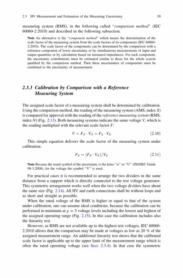
The assigned scale factor of a measuring system shall be determined by calibration.Using the comparison method, the reading of the measuring system (AMS, index X)is compared for approval with the reading of the reference measuring system (RMS,index N) (Fig. 2.13). Both measuring systems indicate the same voltage V, which isthe reading multiplied with the relevant scale factor F:
V ¼ FN � VN ¼ FX � VX ð2:10Þ
This simple equation delivers the scale factor of the measuring system undercalibration:
FX ¼ FN � VNð Þ=VX ð2:11Þ
Note Because the usual symbol of the uncertainty is the letter ‘‘u’’ or ‘‘U’’ (ISO/IEC Guide98-3:2008), for the voltage the symbol ‘‘V’’ is used.
For practical cases it is recommended to arrange the two dividers in the samedistance from a support which is directly connected to the test voltage generator.This symmetric arrangement works well when the two voltage dividers have aboutthe same size (Fig. 2.14). All HV and earth connections shall be without loops andas short and straight as possible.
When the rated voltage of the RMS is higher or equal to that of the systemunder calibration, one can assume ideal conditions, because the calibration can beperformed in minimum at g = 5 voltage levels including the lowest and highest ofthe assigned operating range (Fig. 2.15). In this case the calibration includes alsothe linearity test.
However, as RMS are not available up to the highest test voltages, IEC 60060-2:2010 allows that the comparison may be made at voltages as low as 20 % of theassigned measurement range. An additional linearity test shows that the calibratedscale factor is applicable up to the upper limit of the measurement range which isoften the rated operating voltage (see Sect. 2.3.4). In that case the symmetric
2.3 HV Measurement and Estimation of the Measuring Uncertainty 39
arrangement of the two measuring systems as in Fig. 2.14 is impossible, but oneshould use sufficient clearances (Fig. 2.1) that the RMS is not influenced by theoften much larger system under calibration.
The used RMS shall have a calibration traceable to national and/or internationalstandards of measurement maintained by a National Metrology Institute (NMI)(Hughes et al. 1994; Bergman et al. 2001). This means that RMS calibrated by aNMI or by an accredited calibration laboratory (ACL) with NMI accreditation aretraceable to national and/or international standards. The requirements to RMS aregiven in Table 2.3. The calibration of RMS can be made with transfer RMS(TRMS) of lower uncertainty (UM B 0.5 % for voltage and UM B 3 % for impulsetime parameter measurement). The traceability is maintained by inter-comparisonsof RMS’s of different calibration laboratories (Maucksch et al. 1996).
Calibrations can be performed by accredited HV test laboratories provided thata correctly maintained RMS and skilled personnel are available and traceability isguaranteed. This may be possible in larger test fields, the usual way is to ordercalibration by an ACL.
VXVN
reference measuring system
FN
measuring system under calibration
FX
Fig. 2.13 Principlearrangement of the measuringsystems for calibration usingthe comparison method
Table 2.3 Requirements to reference measuring systems (RMS)
Test voltage DC(%)
AC(%)
LI, SI(%)
Front-choppedLIC (%)
Expanded uncertainty of voltage measurement UM 1 1 1 3Expanded uncertainty of time parameter
measurement UMT
– – 5 5
40 2 Basics of High-Voltage Test Techniques
2.3.4 Estimation of Uncertainty of HV Measurements
The calibration process consists of the described comparisons with n C 10applications on each of the g = 1 to h C 5 voltage levels provided the ratedoperating voltage of the RMS is not less than that of the AMS under calibration(Fig. 2.15). One application means for LI/SI voltage the synchronous readings ofone impulse, for AC/DC voltage the synchronous readings at identical times. Fromeach reading the scale factor according to Eq. (2.11) is calculated and for eachvoltage level Vg, its scale factor Fg is determined as the mean value of the napplications (usually n = 10 applications are sufficient):
Fg ¼1n
Xn
i¼1
Fi;g: ð2:12Þ
Under the assumption of a Gauss normal distribution the dispersion of theoutcomes of the comparisons is described by the relative standard deviation (alsocalled ‘‘variation coefficient’’) of the scale factors Fi:
generatorsupport
system under reference measuringcalibration system
Fig. 2.14 Practicalarrangement for LI voltagecalibration using thecomparison method(Courtesy of TU Dresden)
2.3 HV Measurement and Estimation of the Measuring Uncertainty 41
The standard deviation of the mean value Fg is called the ‘‘Type A standarduncertainty ug’’ and calculated for a Gauss normal distribution by
ug ¼sgffiffiffi
np : ð2:14Þ
After the comparison at all h C 5 voltage levels Vg, the calibrated AMS scalefactorF is calculated as the mean value of the Fg:
F ¼ 1h
Xh
g¼1
Fg; ð2:15Þ
with a Type A standard uncertainty as the largest of those of the different levels
uA¼maxh
g¼1ug: ð2:16Þ
Additionally one has to consider the non-linearity of the scale factor by a TypeB contribution
Note Type A uncertainty contributions to the standard uncertainty are related to thecomparison itself and based on the assumption that the deviations from the mean aredistributed according to a Gauss normal distribution with parameters according to (2.12)and (2.13) (Fig. 2.16a), whereas the Type B uncertainty contributions are based on theassumption of a rectangular distribution of a width 2a with the mean valuexm = (a+ ? a-)/2 and the standard uncertainty u = a/H3 (Fig. 2.16b), details aredescribed in IEC 60060-2:2010 and below in this subsection.
uB0 ¼1ffiffiffi3p �max
h
g¼1
Fg
F� 1
����
����: ð2:17Þ
When the RMS rated operating voltage is lower than that of the AMS undercalibration, IEC 60060-2:2010 allows the comparison over a limited voltage range
F1; u1
F2; u2
F3; u3
F4; u4
F5; u5
voltage
Result according to equations 2.15 to 2.17:
F; u
Fig. 2.15 Calibration overthe full voltage range (IEC60060-2:2010)
42 2 Basics of High-Voltage Test Techniques
(VRMS C 0.2 VAMS) using only a C 2 levels. The comparison shall be completedby a linearity test with b C (6 - a) levels (Fig. 2.17). Then the scale factor F isestimated by
F ¼ 1a
Xa
g¼1
Fg; ð2:18Þ
the standard uncertainty by
uA¼maxa
g¼1ug; ð2:19Þ
and the non-linearity contribution of the calibration by
uB0 ¼1ffiffiffi3p �max
a
g¼1
Fg
F� 1
����
����: ð2:20Þ
Fig. 2.17 Calibration over alimited voltage range andadditional linearity test(IEC60060-2:2010)
1
0
2a
xi σ xi xi σ x0
p(x)
p(x)
2a
a- xi a+ x
2a/√3
(a) (b)
Fig. 2.16 Assumed density distribution functions for uncertainty estimation a Gauss normaldensity distribution for Type A uncertainty. b Rectangular density distribution for Type Buncertainty
2.3 HV Measurement and Estimation of the Measuring Uncertainty 43
An additional non-linearity contribution comes from the range of the linearitytest and shall be calculated as described below under ‘‘non-linearity effect’’.
Example 1 A 1,000 kV LI voltage measuring system (AMS) with a scale factor ofFX0 = 1,000 (calibrated 3 years ago) has shown peak voltage deviations of more than 3 %by comparison with a second AMS during a performance check. Therefore, it has to becalibrated by comparison with a RMS. A 1,200 kV LI reference measuring system (RMS)is available for that calibration. It has been decided to perform the comparison at g = 5voltage levels with n = 10 applications each. The RMS is characterized by a scale factorFN = 1,025 and an expanded uncertainty of measurement of UN = 0.80 %. Table 2.4shows the comparison at the first level. As a result, one gets the scale factor F1 for that firstvoltage level (g = 1) and the related standard deviation s1 and standard uncertainty u1.
Table 2.5 summarizes the results of all five comparison levels and as a finalresult the new scale factor FX and the Type A standard uncertainty uA according tothe Eqs. (2.15) and (2.16).
The uncertainty evaluation of Type B is related to all influences different fromthe statistical comparison. It includes the following contributions to theuncertainty.
Table 2.4 Comparison at the first level V1 & 0.2 Vr
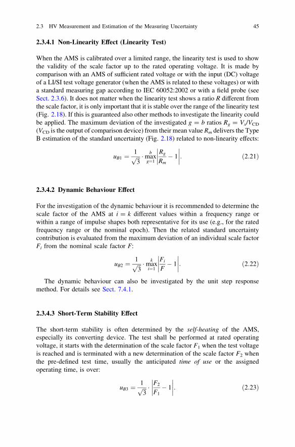
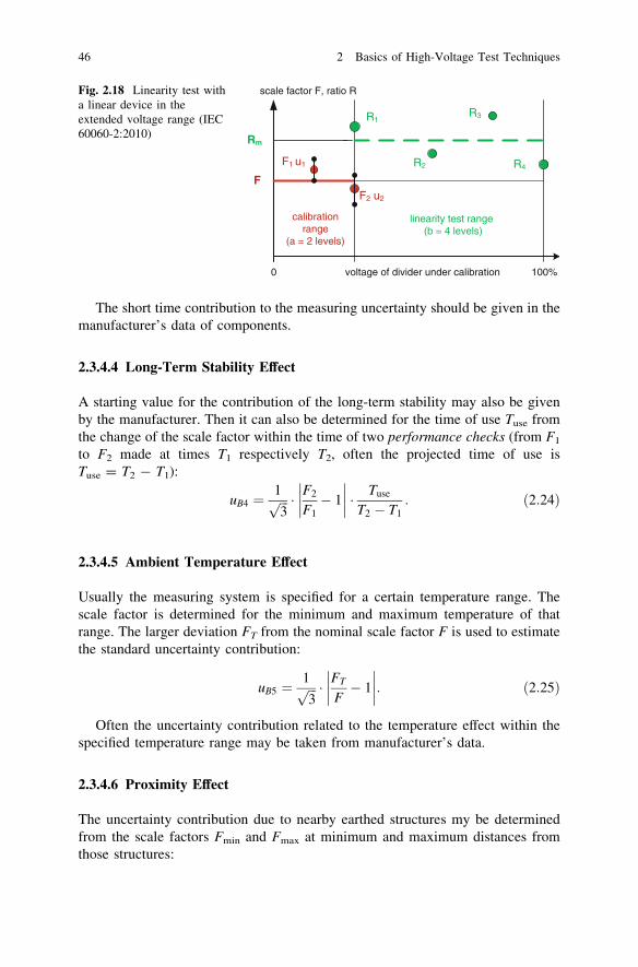
When the AMS is calibrated over a limited range, the linearity test is used to showthe validity of the scale factor up to the rated operating voltage. It is made bycomparison with an AMS of sufficient rated voltage or with the input (DC) voltageof a LI/SI test voltage generator (when the AMS is related to these voltages) or witha standard measuring gap according to IEC 60052:2002 or with a field probe (seeSect. 2.3.6). It does not matter when the linearity test shows a ratio R different fromthe scale factor, it is only important that it is stable over the range of the linearity test(Fig. 2.18). If this is guaranteed also other methods to investigate the linearity couldbe applied. The maximum deviation of the investigated g = b ratios Rg = Vx/VCD
(VCD is the output of comparison device) from their mean value Rm delivers the TypeB estimation of the standard uncertainty (Fig. 2.18) related to non-linearity effects:
uB1 ¼1ffiffiffi3p �max
b
g¼1
Rg
Rm� 1
����
����: ð2:21Þ
2.3.4.2 Dynamic Behaviour Effect
For the investigation of the dynamic behaviour it is recommended to determine thescale factor of the AMS at i = k different values within a frequency range orwithin a range of impulse shapes both representative for its use (e.g., for the ratedfrequency range or the nominal epoch). Then the related standard uncertaintycontribution is evaluated from the maximum deviation of an individual scale factorFi from the nominal scale factor F:
uB2 ¼1ffiffiffi3p �max
k
i¼1
Fi
F� 1
����
����: ð2:22Þ
The dynamic behaviour can also be investigated by the unit step responsemethod. For details see Sect. 7.4.1.
2.3.4.3 Short-Term Stability Effect
The short-term stability is often determined by the self-heating of the AMS,especially its converting device. The test shall be performed at rated operatingvoltage, it starts with the determination of the scale factor F1 when the test voltageis reached and is terminated with a new determination of the scale factor F2 whenthe pre-defined test time, usually the anticipated time of use or the assignedoperating time, is over:
uB3 ¼1ffiffiffi3p � F2
F1� 1
����
����: ð2:23Þ
2.3 HV Measurement and Estimation of the Measuring Uncertainty 45
The short time contribution to the measuring uncertainty should be given in themanufacturer’s data of components.
2.3.4.4 Long-Term Stability Effect
A starting value for the contribution of the long-term stability may also be givenby the manufacturer. Then it can also be determined for the time of use Tuse fromthe change of the scale factor within the time of two performance checks (from F1
to F2 made at times T1 respectively T2, often the projected time of use isTuse = T2 - T1):
uB4 ¼1ffiffiffi3p � F2
F1� 1
����
���� �Tuse
T2 � T1: ð2:24Þ
2.3.4.5 Ambient Temperature Effect
Usually the measuring system is specified for a certain temperature range. Thescale factor is determined for the minimum and maximum temperature of thatrange. The larger deviation FT from the nominal scale factor F is used to estimatethe standard uncertainty contribution:
uB5 ¼1ffiffiffi3p � FT
F� 1
����
����: ð2:25Þ
Often the uncertainty contribution related to the temperature effect within thespecified temperature range may be taken from manufacturer’s data.
2.3.4.6 Proximity Effect
The uncertainty contribution due to nearby earthed structures my be determinedfrom the scale factors Fmin and Fmax at minimum and maximum distances fromthose structures:
calibration range
(a = 2 levels)
linearity test range(b = 4 levels)
0 voltage of divider under calibration 100%
Rm
R1
R2
R3
R4F1 u1
F2 u2
F
scale factor F, ratio RFig. 2.18 Linearity test witha linear device in theextended voltage range (IEC60060-2:2010)
46 2 Basics of High-Voltage Test Techniques
uB6 ¼1ffiffiffi3p � Fmax
Fmin� 1
����
����: ð2:26Þ
The proximity effect for smaller HV measuring systems is often investigated bythe manufacturer of the converting device and can be taken from the manual.
2.3.4.7 Software Effect
When digital measuring instruments, especially digital recorders, are used, acorrect measurement is assumed when artificial test data (which are given in IEC61083-2:2011) are within certain tolerance ranges, also given in IEC 61083-2:2011. It should not be neglected that there may be remarkable standard uncer-tainty contributions caused by that method. The assumed uncertainty contributionby the software is only related to the maximum width of these tolerance ranges Toi
given in IEC 61083-2:
uB7 ¼1ffiffiffi3p �max
n
i¼1Toið Þ: ð2:27Þ
Note Only those tolerance ranges Toi of artificial test data similar to the recorded impulsevoltage must be taken into consideration.
Example 2 The AMS characterized in the first example is investigated with respect to theType B standard uncertainty contributions. For the uncertainty estimation of the calibra-tion also the standard uncertainties of the RMS which are not included in its measuringuncertainty must be considered. Table 2.6 summarizes both and mentions the source of thecontribution.
Table 2.6 Type B uncertainty contributions
Uncertaintycontribution
Symbol ofcontribution
Uncertainty contribution forRMS
Uncertainty contribution forAMS
Non-linearity effectEq. (2.22)
uB1 included in calibration:uN = UN/2 = 0.4 %
included in calibrationuA
Dynamic behavioureffect Eq. (2.23)
uB2 included in calibration 0.43 % from deviationwithin nominal epoch
Short-term stabilityeffect Eq. (2.24)
uB3 included in calibration 0.24 % from deviationbefore and after a 3 htest
Long-term stabilityeffect Eq. (2.25)
uB4 included in calibration 0.34 % from consecutiveperformance tests
Ambient temperatureeffect Eq. (2.26)
uB5 0.06 % because outside ofspecified temperaturerange
0.15 % from manufacturersdata
Proximity effect Eq.(2.27)
uB6 included in calibration can be neglected because ofvery large clearances
Software effect Eq.(2.28)
uB7 included in calibration can be neglected because nodigital recorder applied
2.3 HV Measurement and Estimation of the Measuring Uncertainty 47
2.3.4.8 Determination of expanded uncertainties
IEC 60060-2:2010 recommends a simplified procedure for the determination of theexpanded uncertainty of the scale factor calibration and of the HV measurement. Itis based on the following assumptions which meet the situation in HV testing:
• Independence: The single measured value is not influenced by the precedingmeasurements.
• Rectangular distribution: Type B contributions follow an rectangulardistribution.
• Comparability: The largest three uncertainty contributions are of approximatelyequal magnitude.
Note IEC 60060-2:2010 does not require the application of this simplified method, allprocedures in line with the ISO/IEC Guide 98-3:2008 (GUM) are also applicable. In theAnnexes A and B of IEC 60060-2:2010 a further method directly related to the GUM isdescribed.
The relation between the standard uncertainty and the calibrated new scalefactor can be expressed by the term (F ± u) which characterizes a range of pos-sible scale factors (Not to forget, F is a mean value and u is the standard deviationof this mean value!). Under the assumption of a Gauss normal density distribution(Fig. 2.17a) this range covers 68 % of all possible scale factors. For a higherconfidence, the calculated standard uncertainty can be multiplied by a ‘‘coveringfactor’’ k [ 1. The range (FX ± k � u) means the scale factor plus/minus its‘‘expanded uncertainty’’ U = k � u. Usually a coverage factor k = 2 is appliedwhich covers a confidence range of 95 %.
To determine first the expanded uncertainty of the calibrationUcal, the standarduncertainty uN of measurement of the RMS from its calibration, the Type Astandard uncertainty from the comparison and the Type B standard uncertaintiesrelated to the reference measuring system are combined according to the geometricsuperposition:
The expanded uncertainty of calibration appears on the calibration certificatetogether with the new scale factor. But in case of a HV acceptance test, theexpanded uncertainty of a HV measurement is required. When the AMS is cali-brated and all possible ambient conditions are considered (ambient temperaturerange, range of clearances, etc.), then the expanded uncertainty of HV measure-ment can be pre-calculated by the standard uncertainty of the calibration ucal andthe Type B contributions of the AMS uBiAMS
The pre-calculated expanded uncertainty of measurement should also bementioned on the calibration certificate together with the pre-defined conditions ofuse. The user of the HV measuring system has only to estimate additionaluncertainty contributions when the HV measuring system has to operate outsidethe conditions mentioned in the calibration certificate.
Example 3 For the calibrated AMS the expanded uncertainties of calibration and HVmeasurement shall be calculated under the assumption of certain ambient conditionsmentioned in the calibration certificate. The calculation uses the results of the twoexamples above:
Calibration results:Reference measuring system (RMS):RMS: measuring uncertainty
RMS: temperature effectUN = 0.80 % uN = 0.4 %
uB5 = 0.06 %Calibration by comparison uA = 0.86 %Expanded calibration uncertainty (95 %confidence, k = 2)
Ucal = 1.90 %
Standard uncertainty of calibration ucal = 0.95 %HV measurement:AMS: non-statistical influences uB2 = 0.43 %
uB3 = 0.24 %uB4 = 0. 4 %uB5 = 0.15 %
Expanded uncertainty of measurement (95 %confidence)
UM = 2.26 %
Precise measurement result: V = Vx (1 ± 0.0226)
The HV measuring system shall be adjusted according to its new scale factor ofF = 1.0289 (Table 2.5), possibly with a change of the instrument scale factor tomaintain the direct reading of the measured HV value on the monitor. IEC 60060-2:2010 requires an uncertainty of HV measurement of UM B 3 %. Because ofUM = 2.26 % \ 3 % (Example 3), the system can be used for further HV mea-surement. But it is recommended to investigate the reasons for the relatively highexpanded uncertainty UM for improvement of the measuring system.
2.3.4.9 Uncertainty of Time Parameter Calibration
IEC 60060-2:2010 (Sect. 5.11.2) describes a comparison method for the estimationof the expanded uncertainty of time parameter measurement. Furthermore in its
2.3 HV Measurement and Estimation of the Measuring Uncertainty 49
Annex B.3, it delivers an additional example for the evaluation according to theISO/IEC Guide 98-3:2008. Instead of the consideration of the dimensionless scalefactor for voltage measurement, the method applies to the time parameter (e.g., theLI front time T1X) itself, considers the error of the time measurement T1N by thereference measuring system as negligible and gets from the comparison directlythe mean error DT1,
DT1 ¼1n
Xn
i¼1
T1X;i � T1N;i
� �; ð2:30Þ
the standard deviation
s DT1ð Þ ¼ffiffiffiffiffiffiffiffiffiffiffiffiffiffiffiffiffiffiffiffiffiffiffiffiffiffiffiffiffiffiffiffiffiffiffiffiffiffiffiffiffiffiffiffiffiffiffiffiffi
1n� 1
Xn
i¼1
DT1;i � DT1� �2
s; ð2:31Þ
and the Type A standard uncertainty
uA ¼s DT1ð Þffiffiffi
np : ð2:32Þ
The Type B contributions to the measuring uncertainty of time parameters aredetermined as maximum differences between the errors of individual measure-ments and the mean error of the time parameter T1 for different LI front times, e.g.,the two limit values of the nominal epoch of the measuring system.
For external influences, the procedure of the Type B uncertainty estimationfollows the principles described above for voltage measurement Eqs. (2.22–2.27).For the expanded uncertainty of time calibration and time parameter measurementan analogous application of Eqs. (2.28) and (2.29) is recommended.
A performance test includes the calibration of the scale factor, for impulsevoltages also of the time parameters, and the described full set of tests of theinfluences on the uncertainty of measurement. The data records of all tests shall beincluded to the record of performance. The comparison itself and its evaluation canbe aided by computer programs (Hauschild et al. 1993).
2.3.5 HV Measurement by Standard Air Gaps Accordingto IEC 60052:2002
The breakdown voltages of uniform and slightly non-uniform electric fields, ase.g., those between sphere electrodes in atmospheric air, show high stability andlow dispersion. Schumann (1923) proposed an empirical criterion to estimate thecritical field strength at which self-sustaining electron avalanches are ignited. If
50 2 Basics of High-Voltage Test Techniques
modified, this criterion can also be used to calculate the breakdown voltage Vb ofuniform fields versus the gap spacing S. For a uniform electric field in air atstandard conditions the breakdown voltage can be approximated by the empiricalequation
Vb=kV ¼ 24:4 Sþ S
13:1 cm
� �0:5" #
: ð2:33Þ
This equation is applicable for sphere gaps if the spacing is less than one-thirdof the sphere diameter Fig. (2.19).
Based on such experimental and theoretical results, sphere-to-sphere gaps areused for peak voltage measurement since the early decades of the twentieth cen-tury (Peek 1913; Edwards and Smee 1938; Weicker and Hörcher 1938; Hagenguthet al. 1952) and led to the first standard of HV testing, the present IEC 60052:2002.Meanwhile it is fully understood that this applicability is based on the so-calledstreamer breakdown mechanism, e.g., Meek (1940), Pedersen (1967), and break-down voltage-gap distance characteristics of sphere gaps can also be calculatedwith sufficient accuracy (Petcharales 1986).
For a long time measuring sphere gaps with gap diameters up to 3 m formedthe impression of HV laboratories. But the voltage measurement by sphere gaps isconnected with the breakdown of the test voltage therefore their application is notsimple. Furthermore they need a lot of clearances (see below), well maintainedclean surfaces of the spheres and atmospheric corrections (see Sect. 2.1.2) formeasurement according to the standard.
Today they are not used for daily HV measurement and do not play the sameimportant role in HV laboratories as in the past. Their main application is forperformance checks of AMSs (see Sect. 2.3.2) or linearity checks (see Sect. 2.3.4).For acceptance tests on HV apparatus the inspector may require a check of theapplied AMS by a sphere gap to show that it is not manipulated. For theseapplications mobile measuring gaps with sphere diameters D B 50 cm aresufficient.
The IEC Standard on voltage measurement by means of sphere gaps has beenthe oldest IEC standard related to HV testing. Its latest edition IEC 60052Ed.3:2002 describes the measurement of AC, DC, LI and SI test voltage withhorizontal and vertical sphere-to-sphere gaps with sphere diameters D = (2 …200 cm) and one of the spheres earthed. The spacing S for voltage measurement isrequired S B 0.5 D, for rough estimations it can be extended up toS = 0.75 D. The surfaces shall be smooth with maximum roughness below 10 lmand free of irregularities in the region of the sparking point. The curvature has tobe as uniform as possible, characterized by the difference of the diameter of nomore than 2 %. Minor damages on that part of the hemispherical surface, which isnot involved in the breakdown process, do not deteriorate the performance of themeasuring gap. To avoid erosion of the surface of the sphere after AC and DCbreakdowns, pre-resistors may be applied of 0.1–1 M9X.
2.3 HV Measurement and Estimation of the Measuring Uncertainty 51
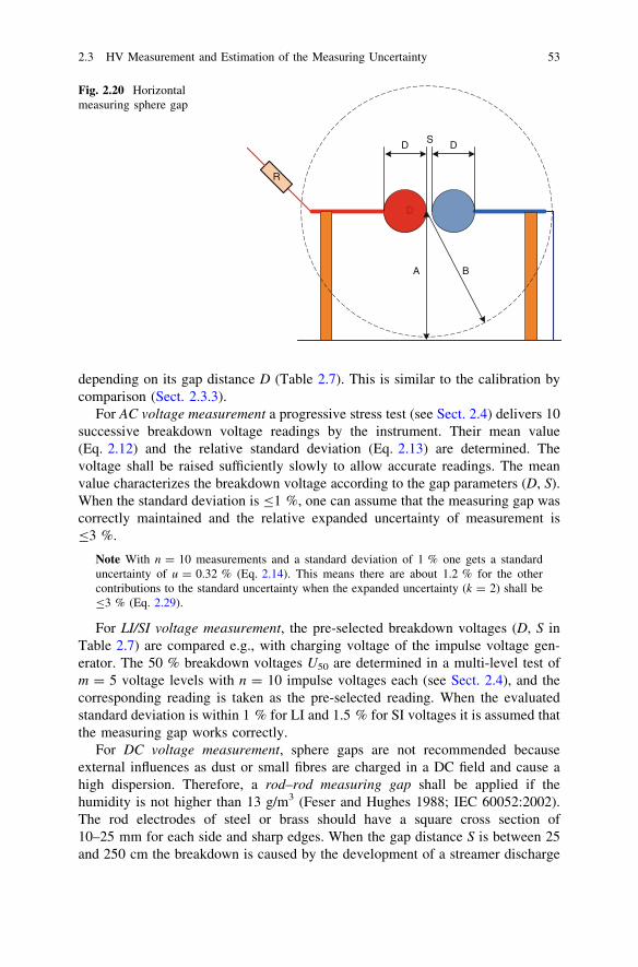
Surrounding objects may influence the results of sphere gap measurements.Consequently the dimensions and clearances for standard air gaps are prescribedin IEC 60052 and shown in Figs. 2.19 and 2.20. The required range of the height Aabove ground depends on the sphere diameter, and is for small spheres A = (7 …9) D and for large spheres A = (3 … 4)�D. The clearance to earthed externalstructures depends on the gap distance S, and shall be between B = 14 S for smalland B = 6 S for large spheres.
The dispersion of the breakdown voltage of a measuring gap depends stronglyfrom the availability of a free starting electron, especially for gaps withD B 12.5 cm and/or measurement of peak voltages Up B 50 kV. Starting elec-trons can be generated by photo ionization (Kuffel 1959; Kachler 1975). Thenecessary high energy radiation may come from the far ultra-violet (UVC) contentof nearby corona discharges at AC voltage, or from the breakdown spark of theopen switching gaps of the used impulse generator, or a special mercury-vapourUVC lamp with a quartz tube.
Note In the past, even a radioactive source inside the measuring sphere has been applied.For safety reasons this is forbidden now.
Table 2.7 gives the relationship of the measured breakdown voltage Ub
depending on the distance S between electrodes for some selected sphere diametersD B 1 m which are mainly used for the mentioned checks, for other spherediameters see IEC 60052:2002. A voltage measurement with a sphere gap meansto establish a relation between an instrument at the power supply input of the HVG(e.g., a primary voltage measurement at the input of a test transformer) and theknown breakdown voltage of the standard measuring gap in the HV circuit
D
D
S
B
A
R
Fig. 2.19 Verticalmeasuring sphere gap(explanations in the text)
52 2 Basics of High-Voltage Test Techniques
depending on its gap distance D (Table 2.7). This is similar to the calibration bycomparison (Sect. 2.3.3).
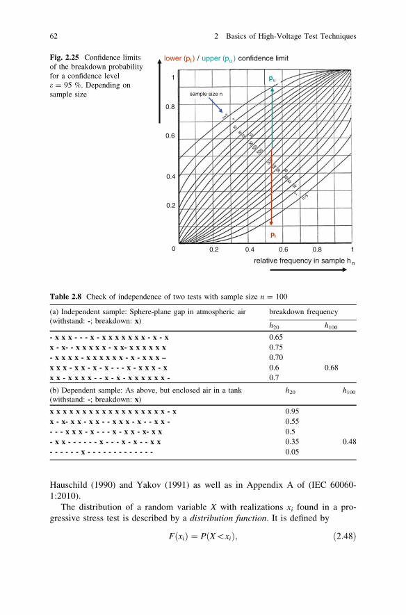
For AC voltage measurement a progressive stress test (see Sect. 2.4) delivers 10successive breakdown voltage readings by the instrument. Their mean value(Eq. 2.12) and the relative standard deviation (Eq. 2.13) are determined. Thevoltage shall be raised sufficiently slowly to allow accurate readings. The meanvalue characterizes the breakdown voltage according to the gap parameters (D, S).When the standard deviation is B1 %, one can assume that the measuring gap wascorrectly maintained and the relative expanded uncertainty of measurement isB3 %.
Note With n = 10 measurements and a standard deviation of 1 % one gets a standarduncertainty of u = 0.32 % (Eq. 2.14). This means there are about 1.2 % for the othercontributions to the standard uncertainty when the expanded uncertainty (k = 2) shall beB3 % (Eq. 2.29).
For LI/SI voltage measurement, the pre-selected breakdown voltages (D, S inTable 2.7) are compared e.g., with charging voltage of the impulse voltage gen-erator. The 50 % breakdown voltages U50 are determined in a multi-level test ofm = 5 voltage levels with n = 10 impulse voltages each (see Sect. 2.4), and thecorresponding reading is taken as the pre-selected reading. When the evaluatedstandard deviation is within 1 % for LI and 1.5 % for SI voltages it is assumed thatthe measuring gap works correctly.
For DC voltage measurement, sphere gaps are not recommended becauseexternal influences as dust or small fibres are charged in a DC field and cause ahigh dispersion. Therefore, a rod–rod measuring gap shall be applied if thehumidity is not higher than 13 g/m3 (Feser and Hughes 1988; IEC 60052:2002).The rod electrodes of steel or brass should have a square cross section of10–25 mm for each side and sharp edges. When the gap distance S is between 25and 250 cm the breakdown is caused by the development of a streamer discharge
D
DD
DS
BA
R
Fig. 2.20 Horizontalmeasuring sphere gap
2.3 HV Measurement and Estimation of the Measuring Uncertainty 53
of a required average voltage gradient e = 5.34 kV/cm. Then the breakdownvoltage can be calculated by
Vb=kV ¼ 2þ 5:34 � S=cm: ð2:34Þ
The length of the rods in a vertical arrangement shall be 200 cm, in a horizontalgap 100 cm. The rod–rod arrangement should be free of PD at the connection ofthe rods to the HV lead, respectively to earth. This is realized by toroid electrodesfor field control. For a horizontal gap the height above ground should be C400 cm.The test procedure is as that for AC voltages described above.
2.3.6 Field Probes for Measurement of High Voltagesand Electric Field Gradients
The ageing of the insulation and thus the reliability of HV apparatus is mainlygoverned by the maximum electrical field strength. Even if the field distribution in
Table 2.7 Peak value of breakdown voltages of selected standard sphere gaps
Gapdistance
50 % breakdown voltage Vb50/kV at sphere diameter D/mmb
Explanations:a For measurement of DC test voltages [130 kV standard sphere gaps are not recommended,apply rod–rod gaps and see Eq. (2.34)b For correctly maintained standard sphere gaps, the expanded uncertainty of measurement ofAC, LI and SI test voltages is assumed to be UM & 3 % for a confidence level of 95 %. There isno reliable value for DC test voltagesc The values in brackets are for information, no level of confidence is assigned to them
54 2 Basics of High-Voltage Test Techniques
dielectric materials can well be calculated based on the Maxwell equations usingadvanced computer software, the validity of the theoretical results should bevalidated experimentally. For this purpose capacitive sensors, commonly referredto as field probes, can be used. The field distribution, however, may substantiallybe affected by the presence of such field probes which should thus be designed assmall as possible to minimize the field distortion und thus the inevitable measuringuncertainty (Les Renardieres Group 1974; Malewski et al. 1982). In specific cases,however, field probes can be designed such that the field is not disturbed, as in thecase of coaxial electrode configurations representative for bushings, power cablesand SF6 switchgears. Moreover, field probes can be integrated in the earth elec-trode of a plane-to-plane electrode arrangement of Rogowski profile, as sketchedin Fig. 2.21. Under this condition the voltage applied to the HV electrode cansimply be deduced from the field strength at the sensing electrode.
The fundamental measuring principle is based on the first Maxwell equationwhich reads:
rot~H ¼ o~D=ot þ ~G; ð2:35Þ
with ~H—vector of the magnetic field strength, ~D—vector of the electric dis-
placement flux density, ~G—vector of the current density at the sensor electrode.For gaseous dielectrics the conductivity is extremely low so that the second
term in Eq. (2.35) can be neglected:
rot~H ¼ o~D=ot; ð2:36aÞ
In contrast to this the conductivity of the sensing electrode is extremely high sothat for this case the first term in Eq. (2.35) can be neglected:
rot~H ¼ ~G; ð2:36bÞ
Combining the Eqs. (2.36a and 2.36b) and substituting the density of the dis-placement flux by the electrical field strength, i.e., ~D ¼ e �~E; one gets
~G ¼ o~D=ot ¼ e � o~E=ot; ð2:37Þ
with e—permittivity of the dielectric between both electrodes.For the here considered homogenous field configuration the field gradient
occurs perpendicular to the surface of the sensing electrode. Thus, instead of thevector presentation the simple scalar presentation valid for one dimensional con-figurations is applicable. Consequently the current I(t) captured by the sensor cansimply be expressed by the current density G multiplied with the area A of thesensing electrode:
IðtÞ ¼ A � G ¼ A � e � dEðtÞ=dt: ð2:38Þ
To convert the current induced at the sensor surface into an equivalent voltagesignal Vm(t) it is a common practice to connect the sensor via a measuring
2.3 HV Measurement and Estimation of the Measuring Uncertainty 55
capacitance Cm to earth potential, see Fig. 2.21. As this provides a capacitivevoltage divider, the time-dependent voltage Vh(t) applied to the HV electrode cansimply be determined from the voltage Vm(t) measurable across Cm using thefollowing equation:
VhðtÞ ¼dg�Cm
A � e � VmðtÞ ¼ Sf � VmðtÞ; ð2:39Þ
with Sf—scale factor, dg—gap distance.In principle the measuring capacitance Cm shown in Fig. 2.21 could also be
replaced by a resistor, in the following denoted as Rm. Under this condition onegets from Eq. (2.38):
VmðtÞ ¼ Rm � A � e � dEðtÞ=dt: ð2:40Þ
Based on this, the peak voltage Vhp applied to the top electrode can be deter-mined by
Vhp ¼dg
Rm � A � e� Z
t
0
VmðtÞdt ¼ dg
Rm � A � e � 2pf� Vmp ¼ Sf � Vmp ð2:41Þ
From this equation follows that the scale factor Sf is inversely proportional to thetest frequency f, so that not only Rm but also the test frequency f must be exactlyknown, to determine the peak value of the applied high voltage from the measuredlow voltage, where harmonics should not appear because they may cause severemeasuring errors.
Example Consider an arrangement according to Fig. 2.21 in ambient air with e0 = 8.86pF/V m. Assuming a gap distance dg = 10 cm and an area of the sensing electrodeAs = 10 cm2 as well as a capacitance Cm = 2 nF, one gets the following scale factor:
Sf ¼dg � Cm
A � e0¼ 10 cmð Þ � 2 nFð Þ
10 cm2ð Þ � 8:86 pF/mð Þ ¼ 22:6� 103:
CM
dgE(t)
i(t)
HV electrode
sensing electrode
guard electrode
measuring capacitor
Fig. 2.21 Principle of a fieldprobe for measurements ofhigh alternating voltages
56 2 Basics of High-Voltage Test Techniques
If, for instance, a low voltage of Vm = 5 V across Cm is measured, the appliedhigh voltage becomes Vm = 113 kV. Substituting the capacitor Cm by a measuringresistor of Rm = 500 kX and assuming a test frequency f = 50 Hz, one gets thefollowing scale factor:
Sf ¼dg
Rm � As � e0 � 2pf¼ 18� 103:
The curves plotted in the graph according to Fig. 2.22, which are based on theabove calculations, enable a simple determination of the applied high voltage Vh
from the measured low voltage Vm. In this context it has to be taken into accountthat the scale factor is dependent on the test frequency, if a measuring resistor isused.
The main disadvantage of the arrangement shown in Fig. 2.21 is that it is onlycapable for measuring the field gradients occurring adjacent to earth potential. Tomeasure also arbitrarily oriented field vectors in the space between HV and LVelectrodes, spherical sensors are employed (Feser and Pfaff 1984). As illustrated inFig. 2.23a, the surface of such a sphere is subdivided into six partial sensors toreceive the three cartesian components of the electromagnetic field. To minimizethe inevitable field disturbance caused by the metallic probe, it is battery poweredand the whole components required for signal processing are integrated in thehollow sphere. The evaluated data are transmitted to earth potential via a fiberoptic link. An essential benefit of the spherically shaped probe is that the admis-sible radius depending on the field strength to be measured can be calculatedwithout large expenditure.
Practical realized spherical field probes are capable for measuring fieldstrengths up to about 1 kV/cm where the measuring frequency ranges betweenapprox. 20 Hz and 100 MHz. The application is not only restricted to field strengthmeasurements. If calibrated with a reference measuring system it can also beemployed for high voltage measurements if the field is free of space charges whichcould be caused by corona discharges.
As the field probe provides a capacitive sensor it has to be taken into accountthat the induced charge and thus the measurable current i(t) is a consequence of thedisplacement flux which is correlated with the time dependent field strength E(t).Thus, only time dependent voltages, such as LI, SI, AC and other transients,induce a measurable displacement current. To measure also DC voltages, thedesired alternating displacement current could be generated if the sensing elec-trode is periodically shielded by a rotating electrode connected to earth potential.This approach, schematically shown in Fig. 2.23b, is applied by the so-called fieldmill (Herb et al. 1937; Kleinwächter 1970). Here the sensing electrode is estab-lished by two half-sectioned discs providing the measuring electrodes, which mustbe well isolated from each other. The vane electrode is connected to the guardelectrode on earth potential. If the vane electrode is rotating in front of the mea-suring electrodes, an alternating displacement flux exposes these both electrodes
2.3 HV Measurement and Estimation of the Measuring Uncertainty 57
and induces thus an alternating current. This is correlated with the electrostaticfield strength on the electrode surface which is usually indicated by means of ahigh sensitive amplifier, where the input impedance must be extremely high.
Another option for the measurement of high DC voltages by means of a fieldprobe is the replacement of the electrical method by a mechanical one. That meansthe measuring impedance Cm shown in Fig. 2.21 is replaced by a sensitive forcemeasurement system, as first applied by Kelvin in 1884 for absolute measurementof DC voltages. The principle applied is based on the Coulomb law discovered in1785. For a homogeneous field the force attracting the sensing electrode of an areaA if subjected to a field gradient E can be expressed by:
Fe ¼12� e � A � E2: ð2:42Þ
Example If, for instance, a voltage of Vh = 100 kV is applied to the top electrode and thegap distance is dg = 10 cm, then the field strength at the sensing electrode achieves10 kV/cm. Inserting these values in Eq. (2.42), the force attracting the sensing electrodebecomes Fe & 3.5 9 10-2 N & 3.6 p.
The torsion due to the attracted sensing electrode is usually amplified and indi-cated by a spot light and mirror system. As the electric force is proportional to thequadratic value of the field gradient and thus also proportional to the quadratic valueof the applied test voltage, the indication is independent from the polarity. Thus,electrostatic voltmeters are capable not only for DC voltage measurements but alsofor measuring the r.m.s. value of HVAC test voltages, as treated in Sect. 3.4.
2.4 Breakdown and Withstand Voltage Tests and TheirStatistical Treatment
Electrical discharges and breakdown of insulations are stochastic processes whichmust be described by statistical methods. This subsection gives an introduction to
0
50
100
150
200
250
0 2 4 6 8 10ap
plie
d hi
gh v
olta
ge [k
V]
measured low voltage [V]
Cm = 500 pF
Rm= 500 kΩ
Fig. 2.22 Applied highvoltage versus low voltagemeasurable across acapacitive respectively aresistive measuringimpedance using parametersgiven in the text
the planning, performing and evaluation of HV tests on a statistical basis. Itdescribes tests with voltages increasing up to the breakdown (‘‘progressive stressmethod’’) and with multiple application of pre-given voltages and estimation ofbreakdown probabilities (‘‘multiple level method’’, ‘‘up-and-down method’’). Life-time tests of insulation are performed with pre-given voltages, but progressive testdurations and can be evaluated accordingly. Also standardized HV withstand testsare described and valuated from the viewpoint of statistics. The subsection submitsfirst tools for the application of statistical methods and supplies hints to the specialliterature, e.g., (Hauschild and Mosch 1992).
2.4.1 Random Variables and the Consequences
The phenomena of electrical discharges—as most others in nature, society andtechnology—are based on stochastic processes and characterized by their ran-domness (Van Brunt 1981; Hauschild et al. 1982). This is often ignored and onlyan average trend is considered in order to interpret a relationship being investi-gated. Quite often, however, it is not the mean value, but an extreme value thatdetermines the performance of a system. In technology this is often taken intoaccount by applying a ‘‘safety factor’’. A rather better approach is the statisticaldescription of stochastic phenomena. Therefore, HV tests shall be selected, per-formed and evaluated on a statistical basis: They are random experiments (trials)and described by random variables (sometimes also called ‘‘random variates’’).
When a pre-given constant voltage stress—e.g., a certain LI test voltage—isapplied to an insulation—e.g., an air gap—one can observe the random event‘‘breakdown’’ (A) or the complimentary event ‘‘withstand’’(A*). The relativebreakdown frequencyhn(A) is the relation between the number of breakdownsk and the number of applications n
hn Að Þ ¼ k=n: ð2:43Þ
vanelectrode
guardelectrode
measuringelectrode measuring
electrodes
guardelectrode
Fig. 2.23 Field probes using fixed and rotating electrodes
2.4 Breakdown and Withstand Voltage Tests and Their Statistical Treatment 59
The relative withstand frequency follows to
hn A�ð Þ ¼ n� kð Þ=n ¼ 1� hn Að Þ: ð2:44Þ
The relative frequency depends on the number of performed tests (often calledsample size) and the respective test series as shown for the breakdown frequency inFig. 2.24. The relative frequencies vary around a fixed value and reach it as thelimiting value ‘‘breakdown probability’’ p:
limn!1
hn Að Þ ¼ p: ð2:45Þ
The probability of a withstandq follows accordingly
limn!1
hn A�ð Þ ¼ q: ð2:46Þ
Because a characteristic value of withstand cannot be measured (‘‘Nothinghappens!’’), the withstand probability is determined from the complementarybreakdown probability q = 1 - p. Consequently the statistical definition of awithstand voltage is a voltage which causes a breakdown with low probability,usually p B 0.10. The relative breakdown frequency is a point estimation of thebreakdown probability.
The larger the number of applications for the estimation of the frequency, thebetter is the adaptation of the estimate to the true, but unknown probability(Fig. 2.24). A confidence estimation delivers a feeling for the accuracy of theestimation by the width of the calculated confidence region. This region covers thetrue but unknown value of p with a certain confidence level, e.g., e = 95 %. Fromthe sample the upper and the lower limit of the confidence region are determined onthe basis of the assumption of a theoretical distribution function, in this case basedon the binomial distribution function and the Fisher (F) distribution as testdistribution.
Explanation: The binomial distribution is based on two complementary eventsA and A* (as breakdown and withstand) occurring with the known probabilitiesp and q (Bernoulli trial). The binomial distribution indicates the probabilityP(X = k) with which the event A will occur k-times in n independent trials.
P X ¼ kð Þ ¼ nk
� �pk 1� pð Þn�k ð2:47Þ
where k ¼ 0; 1; 2; . . .; n and
nk
� �¼ n!
k! � n� kð Þ!¼n � n�1ð Þ � . . . n� kþ1ð Þ
1 � 2 � 3 � . . . � k
Figure 2.25 shows the 95 % confidence limits depending on the relativebreakdown frequency and the number of applications (sample size).
Example For hn(A) = 0.7 and n = 10 applications, Fig. 2.25 delivers the lower limitpl = 0.37 and the upper limit pu = 0.91. With a statistical confidence e = 95 %, the realprobability is within a range of 0.37 B p B 0.91. For n = 100 applications one would get
60 2 Basics of High-Voltage Test Techniques
the much smaller range 0.60 B p B 0.78. Again, with increasing sample size the esti-mation becomes better, this means the confidence region becomes smaller.
When a constant voltage test has been performed for the estimation of thebreakdown probability, it must be checked whether the test is ‘‘independent’’ ornot. Independence means that the previous voltage applications have no influenceon the result of the application under consideration. This can be shown by theinvestigation of the trend (Table 2.8). A sample of n = 100 is subdivided into fivesamples of n* = 20 each. If the relative frequencies of the sub-samples scatteraround that of the whole sample, it could be considered as independent (case a). Ifthere is a clear trend (case b) it would be dependent and any statistical evaluation isforbidden. Independence can only be ensured due to an improvement of the testprocedure, e.g., breaks of sufficient duration between single stresses. Furtherdetails of constant voltage tests are described in (Hauschild and Mosch 1992).
There is a second group of HV breakdown tests with increasing stress, e.g.,continuously raising AC or DC test voltages or LI or SI voltages raising in stepsuntil breakdown (Fig. 2.26). Now the breakdown is sure, but the height of thebreakdown voltage is random. This group of tests is called ‘‘progressive stresstests’’. The random variable is the breakdown voltage Vb. But in life-time tests atconstant voltage, the time-to-breakdown Tb becomes the random variable. In bothcases we have a continuous variable.
Note In case of stepwise increasing voltages, the starting value may be varied to getcontinuous outputs (realizations) of the random variable.
The evaluation of progressive stress tests follows the typical treatment ofrandom variables in mathematical statistics as described in many text books ase.g., by Mann et al. (1974), Müller et al. (1975), Storm (1976) or Vardeman(1994). Descriptions especially related to HV tests are given by Lalot (1983),Hauschild and Mosch (1984) (in German) and (1992) (in English), Carrara and
p(A)
hn(A)
10 20 30 40 50 600
0.2
0.4
0.6
0.8
1.0
number of test
relative breakdown frequency
test series 2
test series 1
Fig. 2.24 Relativebreakdown frequencies oftwo test series depending onthe number of tests performed
2.4 Breakdown and Withstand Voltage Tests and Their Statistical Treatment 61
Hauschild (1990) and Yakov (1991) as well as in Appendix A of (IEC 60060-1:2010).
The distribution of a random variable X with realizations xi found in a pro-gressive stress test is described by a distribution function. It is defined by
F xið Þ ¼ P X\xið Þ; ð2:48Þ
1
0.8
0.6
0.4
0.2
0
lower (pl ) / upper (pu ) confidence limit
0.2 0.4 0.6 0.8 1
relative frequency in sample h n
pl
pu
sample size n
Fig. 2.25 Confidence limitsof the breakdown probabilityfor a confidence levele = 95 %. Depending onsample size
Table 2.8 Check of independence of two tests with sample size n = 100
(a) Independent sample: Sphere-plane gap in atmospheric air(withstand: -; breakdown: x)
breakdown frequency
h20 h100
- x x x - - - x - x x x x x x x - x - x 0.65x - x- - x x x x x - x x- x x x x x x 0.75- x x x x - x x x x x x - x - x x x – 0.70x x x - x x - x - x - - - x - x x x - x 0.6 0.68x x - x x x x - - x - x - x x x x x x - 0.7
(b) Dependent sample: As above, but enclosed air in a tank(withstand: -; breakdown: x)
h20 h100
x x x x x x x x x x x x x x x x x x - x 0.95x - x- x x - x x - - x x x - x - - x x - 0.55- - - x x x - x - - - x - x x - x- x x 0.5- x x - - - - - - x - - - x - x - - x x 0.35 0.48- - - - - - x - - - - - - - - - - - - - 0.05
62 2 Basics of High-Voltage Test Techniques
and it indicates the probability P with which the random variable X will assume avalue below the considered value xi. A distribution function (Fig. 2.27) is anymathematical function with the following properties:
0 B F(xi) B 1 (realizations between impossible and sure events),F(xi) B F(xi+1) (monotonously increasing),lim
x!�1FðxÞ ¼ 0 and lim
x!þ1FðxÞ ¼ 1 (boundary conditions).
Note Instead of the distribution function also the density function delivers a completemathematical description, but it is not meaningful for HV test evaluation.
A distribution function is characterized by parameters describing the meanvalue and the dispersion, sometimes in addition to the position of the function. Theevaluation of a progressive stress test means the selection of a well adapted type ofdistribution function and the estimation of its parameters. The parameter estima-tion can be made as a point or confidence estimation based on formulas of func-tional parameters (e.g., the mean value), quantiles (realization of the randomvariable related to a pre-given probability) or intervals (difference between twoquantiles) (Fig. 2.27).
2.4.2 HV Tests Using the Progressive Stress Method
The progressive stress method (PSM) with continuous increasing voltage shall beconsidered for an electrode arrangement in SF6 gas (Fig. 2.26a). The initial voltagev0 must be low enough to avoid any influence on the result, the rate of rise of thevoltage shall be so that a reliable voltage measurement can be performed, and theinterval between two individual tests shall guarantee the independence of therealizations vb. The independence may be checked by a graphic plot of the mea-surements. Other independence tests are described in the above mentionedliterature.
Example Figure 2.28 shows the sequence of four test series at four different pressures ofthe SF6 gas. A series is considered to be independent if the realizations fluctuate in arandom manner around a mean value. A dependence must be assumed, if there is a falling,raising or periodically fluctuating tendency. According to this simple rule, the series at gaspressures of 0.40, 0.25, and 0.15 MPa can be considered as independent and are wellsuited for a statistical evaluation. That at 0.10 MPa is dependent and shall not be statis-tically evaluated. The reason for the dependence should be clarified and the series repeatedunder improved conditions.
Each independent series shall be evaluated statistically, this means graphicallyrepresented and approximated by a theoretical distribution function. Both tasks canbe connected when a so-called probability grid is used for the representation. Aprobability grid uses the inverse function of the considered theoretical distributionfunction on the ordinate. For each type of theoretical distributions, a probability
2.4 Breakdown and Withstand Voltage Tests and Their Statistical Treatment 63
grid can be constructed. Any empirical distribution of the same type as the gridappears as a straight line.
The following theoretical distribution functions are recommended for HVapplications:
The Gauss or normal distribution is characterized by the parameters l (esti-mated by the arithmetic mean value or the 50 % quantile u50) and the standarddeviation r [estimated by the mean square root of (xi - l) or the difference ofquantiles (x84 - x50) = (x50 - x16)]:
F x; l; r2� �
¼ 1ffiffiffiffiffiffiffiffi2prp
Zx
�1
e�z�r2ð Þ2r2 dz: ð2:49Þ
The application of a certain distribution function should be based on its sto-chastic model: A normal-distributed random variable is the result of a large
Fig. 2.26 Procedures ofprogressive stress tests. aContinuous increasing AC orDC voltage. b Stepwiseincreasing AC or DC voltage.c Stepwise increasing LI or SIvoltage
64 2 Basics of High-Voltage Test Techniques
number of independent, randomly distributed influences when each of these makesonly an insignificant contribution to the sum. This model is very well applicable tomany random events, also to breakdown processes with partial discharges.
The Gumbel or double exponential distribution is—as the normal distribution—an unlimited function (-?\ x \ ? ?) characterized by two parameters, its63 % quantile g and the dispersion measure c [estimated by c = (x63 - x05)/3]:
F x; g; cð Þ ¼ 1� e�ex�gc: ð2:50Þ
Stochastic model: The double exponential distribution describes the distributionof realisations according to an extreme value, in case of HV tests it is the minimumof the electric strength. It is a mathematical description of the simple fact that ‘‘thebreakdown of a slightly uniform electric field takes place at the weakest point’’. Itcan be well applied if there are slightly uniform insulations which show a quitehigh dispersion (Mosch and Hauschild 1979).
The Weibull distribution is also a distribution describing extreme values, but itis limited and characterized by three parameters, its 63 % quantile g = x63, theWeibull exponent d as a measure of dispersion and the initial value x0
F x; g; d; x0ð Þ ¼ 1� e�x�x0
gð Þd x [ x0; ð2:51aÞ
F x; g; d; x0ð Þ ¼ 0 x� x0; ð2:51bÞ
d ¼ 1:2898= log x63=x05ð Þ: ð2:51cÞ
x1 xp a b
x1 a b
1
0.8
0.6
0.4
0.2
0
0.4
0.2
0
F(a)
F(b)
F(x)=p
F(x1)
probability
density of probability
random variable
Fig. 2.27 Distribution (a)and density (b) function withthe definitions of quantile x1
and probability interval(F(b) - F(a))
2.4 Breakdown and Withstand Voltage Tests and Their Statistical Treatment 65
The Weibull distribution is highly adaptable in its structure and thereforeapplicable for many problems (Cousineau 2009). For the case x0 = 0 it is the idealfunction for breakdown time investigation (two-parameter Weibull distribution),see e.g., Bernard (1989) and Tsuboi et al. (2010). In the case x0 [ 0, the initialvalue becomes an absolute meaning, e.g., as an ideal withstand voltage of thebreakdown probability p = 0! Therefore consequences must be carefully consid-ered when it is applied to breakdown voltage problems.
For all three theoretical distribution functions a probability grid can be con-structed. Figure 2.29 shows the comparison of the different ordinates of these grids.It can be seen that in the region x15–x85 the grids are very similar, but for very lowand very high probabilities remarkable differences exist. This means that for esti-mation of withstand voltages the correct selection of a theoretical distributionfunction for the adaptation of empirical data (test results) is very important.
In HV tests the empirical distribution function is usually determined from a quitelimited number of realizations, e.g., 10 B n B 100. In that case it is recommendedto arrange the realisations xi according to increasing magnitude between xmin andxmax and to complete them by their relative, cumulative frequencies
hRi ¼Xi
m¼1
hm
nþ 1ð Þ ð2:52Þ
where n is the total number of realizations and hm is the absolute frequency of themth voltage value (Eq. 2.43). Then the data are plotted as a ‘‘stair’’ in a suitedprobability grid. If the empirical (stair) function can be approximated by a straightline, the adaptation with the theoretical function of the grid is acceptable.
0 20 40 60 80 100 number of single test
250
kV
180
120
60
AC breakdown voltage SF6 gas pressure
0.4 MPa
independent
0.25 MPa
independent
0.15 MPa
Independent
0.1 MPa
dependent
Fig. 2.28 Graphical check of independence of four test series in SF6 gas
66 2 Basics of High-Voltage Test Techniques
Example Figure 2.30 shows, the stair function can be well adapted by a straight line in theGauss grid of a normal distribution. This means a normal distribution describes the ran-domness of the performed test sufficiently. Its parameters can be estimated by quantiles:The mean value by u50 = 953 kV and the standard deviation by s = u50 -
u16 = 18.2 kV.
A confidence estimation of the parameters can be performed using so-called testdistributions, the t-distribution for confidence estimates of the mean value and thev2-distribution for the standard deviation. For details see e.g., Hauschild andMosch (1992).
The maximum likelihood method delivers the most efficient estimation ofparameters including their confidence limits. As the term ‘‘likelihood’’ is a syn-onym for ‘‘probability’’, the method delivers estimates of parameters of theselected distribution function, which are those of maximum probability for thegiven sample. The method has been introduced many years ago, but got its broadapplication with numerical calculations by personal computers (PC). It can beapplied for all classes of HV breakdown tests and any type of theoretical distri-bution function (Carrara and Hauschild 1990; Yakov 1991; Vardeman 1994).
The mathematical calculations are based on the so-called ‘‘likelihood functionL’’. It is proportional to the probability pR to obtain a description of the investi-gated sample (realizations xi with i = 1 … n) using a distribution function, e.g.,with the parameters d1 and d2. The n realizations of the sample are distributed tom levels of the random variable xi (breakdown voltage or time). The likelihoodfunction L is based on the probability pR which is proportional to the product of theprobabilities fRi:
Fig. 2.29 Comparison of ordinates of probability grids with identical 50 % quantiles (logarith-mic abscissa for Weibull distribution)
2.4 Breakdown and Withstand Voltage Tests and Their Statistical Treatment 67
The factor ‘‘A’’ is for normalization only. The most likely point estimates of theparameters d1 and d2 are those which maximize L as shown in Fig. 2.31 (d*1 andd*2). They are calculated from the maximum conditions dL/dd1 = 0 and dL/dd2 = 0, usually performed with the logarithms where the same parametersindicate the maximum
d ln Lð Þ=dd1 ¼ 0 and d ln Lð Þ=dd2 ¼ 0: ð2:54Þ
The three-dimensional diagram shows the likelihood function (L normalized toits maximum) on the area of the two parameters. By help of a cross section throughthe ‘‘likelihood mountain’’ one can define the confidence limits of the parameters(d1min, d1max, d2min, d2max). Each parameter combination of the confidence region(Fig. 2.31) delivers one straight line on the probability grid (Fig. 2.32). The upperand lower border lines of the bundle of straight lines are considered as confidencelimit for the whole distribution function. Figure 2.32 shows this schematically inthe relevant probability grid used for the approximation. The maximum-likelihoodmethod can also be applied to ‘‘censored’’ test results, e.g., when a life-time test isterminated after a certain time and only k of the n test objects have broken down.Then the likelihood function gets the form
0.99
0.9
0.8
0.7
0.6
0.5
0.4
0.3
0.2
0.1
0.01
0.16
0.84
cumulative breakdown frequency h∑
880 900 920 940 960 980 kV 1020
breakdown voltage Vb
s = 18 kV
Vb50 = 952.5 kV
Fig. 2.30 Cumulative frequency distribution function on a Gauss grid
68 2 Basics of High-Voltage Test Techniques
L ¼ A � pR ¼ A �Yk
i¼1
fRi xi=d1; d2ð Þ �Yn�k
i¼kþ1
1� fRi xi=d1; d2ð Þð Þ: ð2:55Þ
The same sample as shown in Fig. 2.30 is evaluated by a commerciallyavailable PC program of the ML method (Speck et al. 2009) under the assumptionof a Weibull distribution (Fig. 2.33). The program delivers after independencetests a plot of the cumulative frequency distribution on a Weibull grid with log-arithmic abscissa. The parameters are estimated as follows: initial valuev0 = 750 kV, 63 % quantile Vb63 = (v0 ? x63) = (750 ? 211) kV and dispersionparameter d = 8.4. The evaluated lower 95 % confidence limit of the cumulativefrequency function should be taken for technical conclusions.
2.4.3 HV Tests Using the Multiple-Level Method
The multiple-level method (MLM) means the application of constant voltage tests(see Sect. 2.4.1) at several voltage levels (Fig. 2.34). For each level the test deliversan estimation of the breakdown probability including its confidence limits (Fig.2.25). The relationship between stressing voltage and breakdown probability is nota distribution function in the statistical sense and therefore called ‘‘performancefunction’’ (sometimes also called ‘‘reaction function’’). The performance functionis not necessarily monotonically increasing, it can decrease (Fig. 2.35), e.g., in caseof a change of the discharge mechanism depending on the height of the voltage. Butit delivers exactly the information necessary for the reliability estimation andinsulation coordination of a power system: The performance function supplies theprobability of a breakdown in case of a certain overvoltage stress.
δ*1
δ1
δ1max
δ1min
δ2maxδ*2δ2min
δ2
L /Lmax
1
K
Fig. 2.31 Point andconfidence estimation by themaximum likelihood function(schematically)
2.4 Breakdown and Withstand Voltage Tests and Their Statistical Treatment 69
In most cases also the performance function shows a monotonic increase andcan be mathematically described by a theoretical distribution function. Figure 2.36shows the difference between the performance function V(x) (simulated by astandardized normal distribution with l = 0 and r = 1) and derived cumulativefrequency functions SDx(x) of different heights Dx of the voltage steps in the test.For statistical reasons, the principle relation is SDx(x) [ V(x). Both functions havea different meaning: cumulative frequency functions consider the probability ofbreakdown at all stresses up to a certain stress value, performance functions do itat a certain stress. Cumulative frequency functions from stepwise increasedvoltages should be converted into performance functions (Hauschild and Mosch1992).
A MLM test shall be performed at m C 5 voltage levels and n C 10 stresses perlevel. The number of stresses is not necessarily identical at all levels. If withstandvoltages are considered, the number of stresses at low breakdown frequency mightbe higher. Then the independence of the outcomes of each level must be checked(see Table 2.8) and confidence estimations for the breakdown probability aredetermined (Fig. 2.25) and plotted in a probability grid.
Example From earlier experiments it can be expected that the performance function ismonotonic increasing and can be approximated by a double exponential distributionfunction. Therefore, the point and confidence estimations are plotted in a Gumbel grid(Fig. 2.37). Because a straight line can be drawn through all confidence regions, theassumption of a double exponential or Gumbel distribution is confirmed. The smallreduction of the relative breakdown frequency between 1,083 and 1,089 kV is not sig-nificant as it can be seen from the confidence limits. The parameters can be estimated fromquantiles, v63 = 1,112 kV and c = (v63 - v31) = 12 kV.
Also the maximum likelihood estimation can be applied when the performancefunction is approximated by a certain distribution function (parameters d1, d2).According to Fig. 2.34 there are j = 1…m voltage levels and apply at each level nj
F(x)
x
50%
x50
lower confidence limit
δ1min
δ*1; δ*2
δ1max
δ2min
δ2max
upper confidence limit
Fig. 2.32 Confidence limitsof the distribution functionderived from Fig. 2.31(schematically)
70 2 Basics of High-Voltage Test Techniques
stresses. The probability of obtaining kj breakdowns and wj = (nj - kj) withstandsat the voltage uj is expressed by the binomial distribution (Eq. 2.47) on the basis ofthe breakdown probabilities given by the performance function V(vj) = V(vj/d1,d2). The corresponding likelihood function for all m voltage levels with nj stressesis given by
0.99
0.9
0.8
0.6
0.4
0.3
0.2
0.1
0.01140 kV
breakdown voltage X = Vb b 0
Cumulative breakdown frequency h∑
0.05
0.63
δ = 8.4(eq. (2.50))
v63 = 211 kV v0 = 750 kV
lower confidence limit
upper confidence limit
260220200180160
-V
Fig. 2.33 Cumulativefrequency function withconfidence limits on Weibullgrid
Fig. 2.34 Test procedureaccording to the multi-levelmethod with m = 8 voltagesteps and n = 10 impulsesper step
2.4 Breakdown and Withstand Voltage Tests and Their Statistical Treatment 71
L ¼Ym
j¼1
V vj=d1; d2� �kj
1� V vj=d1; d2� �� �wj
: ð2:56Þ
Varying the parameters d1 and d2 the maximum of Eq. (2.56) is found asdescribed above. One gets point and confidence estimates as well as a confidenceregion for the whole performance function which is also shown in Fig. 2.33.
For practical applications of the maximum likelihood method the application ofsuitable software is necessary. An optimum software package (Speck et al. 2009)contains all necessary steps of the HV test data evaluation, from several inde-pendence tests, tests for best fitting with a theoretical distribution function, rep-resentation of the empirical performance function (or the cumulative frequencydistribution) on probability grid up to point and confidence estimations for theparameters and the whole performance (or distribution) function.
2.4.4 HV Tests for Selected Quantiles Using the Up-and-Down Method
A whole performance function is not always required, e.g., the withstand voltageof an insulation can be confirmed, when the test voltage value ut is lower than the10 % quantile v10. In that case it is sufficient to determine the value v10, in other
1
0.5
0
breakdown probability
(a) (b)
applied impulse voltage
Fig. 2.35 Performancefunctions with monotonic (a)and non-monotonic (b)increase
SΔ x(x)
-3 -2 -1 0 1 2 x
cumulative frequency relative step height
1 Δx/σ =0,02 0.1 0.2 0.4 0.7 1.0
V(x)
normalized random variable
0.5
Fig. 2.36 Calculatedcumulative frequencyfunctions SDx(x) determinedat different step heights Dx/rbased on an identicalperformance function V(x)
72 2 Basics of High-Voltage Test Techniques
cases it might be sufficient to look for the quantiles v50 or v90. The related up-and-down test method (UDM) which is based on the constant voltage tests (Sect. 3.4.1)has been introduced by Dixon and Mood (1948).
The method requires that the voltage is initially raised in fixed voltage steps Dv,from an initial value v00 at which certainly no breakdown occurs, until a break-down occurs at a certain voltage (Fig. 2.38: v1 is the first counted value). Now thevoltage is reduced by Dv, if no breakdown occurs the voltage is increased in stepsagain until the next breakdown, otherwise in case of breakdown it is reduced byDv. The procedure is repeated until a predetermined number n C 20 of voltagevalues vl, v2, … vn have been obtained. The mean value of these applied voltages isa first estimate for the 50 % breakdown voltagev50:
v50� ¼1n
Xn
l¼1
vl: ð2:57Þ
A more detailed evaluation considers the influence of the step height Dv anduses the number of breakdowns k and the number of withstands q. The sum of the
0.99
0.9
0.8
0.6
0.4
0.3
0.2
0.1
0
1060 1070 1080 1090 1100 1110 kV 1130
= 12 kV
vb63 = 1112 kV
breakdown voltage v b
breakdown probability
lower / upperconfidence limit
0.31
0.63
Y
Fig. 2.37 Performance function with its confidence region according to a ML estimation andconfidence limits of the single breakdown probabilities and a
2.4 Breakdown and Withstand Voltage Tests and Their Statistical Treatment 73
two complimentary events is identical with the number of voltage applicationsn = k ? q starting with the first breakdown. Additionally, the number of voltagelevels or steps vi (with i = 0 … r) is taken into account. It is counted i = 0 fromthe step of the lowest breakdown. On a certain voltage level vi, there are ki
breakdowns. Then the 50 % breakdown voltage can be estimated by
v50 ¼ v0 þ Dv
Pri¼1 i � ki
k� 1
2
� �: ð2:58Þ
Example The test in Fig. 2.38 starts at v00 = 120 kV and has voltage steps of Dv = 5 kV.Including the first breakdown there are l = 20 voltage applications. The first estimate ofv50* by Eq. (2.57) delivers v50* = 145.5 kV.
The lowest voltage level at which a breakdown occurs is v0 = 140 kV. The number ofbreakdowns is k = 9, that of withstands is q = 11 and there are i = 3 voltage steps abovethe lowest breakdown voltage. With these data Eq. (2.58) delivers v50 = 145.3 kV. Thedifference between the two methods is very small, for most practical conclusions it can beneglected.
The UDM test is independent when the single voltage applications do not showa decreasing or increasing mean tendency. A UDM test according to the break-down procedure starts at an initial voltage at which the breakdown is sure and goesdown until the first withstand. It also delivers v50, if the withstands are counted asthe breakdowns above. Furthermore it should be mentioned that there are methodsfor the estimation of the standard deviation of the performance function, but themethod cannot be recommended (see e.g., Hauschild and Mosch 1992). Confi-dence limits shall be calculated by the maximum likelihood function (see below)and not by the only roughly estimated dispersions.
Carrara and Dellera (1972) proposed an ‘‘extended up-and-down-method’’which applies series of stresses (Fig. 2.39) for the determination of pre-selectedquantiles instead of single stresses (Fig. 2.38). For the determination of a certainquantile, a certain number of impulses in one series is necessary. Table 2.9 givesthe relation between the order p of the quantile and the required number ofimpulses in one series. The ‘‘withstand procedure’’ starting with a withstandvoltage v00 and raising the voltage delivers the quantiles vp of the order p B 0.50,the ‘‘breakdown procedure’’ starting with a breakdown voltage and decreasingvoltage to withstands delivers the quantiles of the order p C 0.50.
Figure 2.39b shows the estimation of the statistical withstand voltage deter-mined as the 10 % breakdown voltage (quantile u10) using the withstand proce-dure with n = 7 stresses per series. As soon as only withstands occur in a series,the voltage is increased by Dv to the next higher level. As soon as a breakdownoccurs the voltage is decreased to the next lower level.
When the breakdown procedure is applied, the voltage is decreased when in aseries only breakdowns occur and only increased when the first withstand appears.The expected quantile for this breakdown procedure is v90. The evaluation of thepoint estimation of the quantile can be performed according to the simplifiedevaluation by Eq. (2.57).
74 2 Basics of High-Voltage Test Techniques
Also the computer-aided maximum-likelihood method can be applied for theUDM tests provided related software is available (Speck 1987; Bachmann et al.1991): The principle corresponds to the MLM (see Sect. 2.4.3). For each of the appliedvoltage levels the relative breakdown frequency including its confidence region isestimated (Fig. 2.40 for estimation of v10 with n = 7 stresses per series) and plotted ina suited probability grid (Fig. 2.40: Gauss grid). The maximum of the likelihoodfunction delivers the expected quantile v10 including its confidence limits. The con-fidence region (e = 95 %) of all quantiles is calculated and plotted as a violet line.
2.4.5 Statistical Treatment of Life-Time Tests
A life-time test is the stress of the insulation at a certain constant AC or DC voltage(or a series of impulses). The random variable is the breakdown time (or thenumber of impulses) which can be evaluated according to the PSM (see Sect.2.4.2). When this test is performed at several voltage levels, the relationshipbetween breakdown voltage and breakdown time—usually known as the life-timecharacteristic (LTC)—can be evaluated (Speck et al. 2009). It is described for a p-order quantile of the breakdown voltage vp by
voltage value v / kV: 145 150 145 145 135 145 145 145 155 145 140 150 150 140 140 140 150 150 150 150
step break withst voltage i ki qi ui / kV
3 1 0 155
2 4 2 150 1 3 5 145
0 1 3 140v0
voltage
time
withstand breakdown
Fig. 2.38 Up-and-down method (UDM) for the estimation of the 50 % quantile v50
Table 2.9 Number of stresses n per UDM group for the estimation of the order p of quantiles
n 70 34 14 7 4 3 2 1
p 0.01 0.02 0.05 0.10 0.15 0.20 0.30 0.50 (withstandprocedure)
p 0.99 0.98 0.95 0.90 0.85 0.80 0.70 0.50 (breakdownprocedure)
2.4 Breakdown and Withstand Voltage Tests and Their Statistical Treatment 75
vp ¼ kdt�1=np or tp ¼
kd
vp
� �n
; ð2:59Þ
where tp—p-order quantile of breakdown time, n—life time exponent mainlycharacterizing the insulating material and kd—a constant mainly characterising the
Fig. 2.39 Up-and-down test for the determination of the 90 % quantile v90 (a), and respectivelythe 10 % quantile v10 (b)
76 2 Basics of High-Voltage Test Techniques
field geometry. In a logarithmic grid the formula delivers a falling straight linewhich allows the estimation of the parameters n and kd.
The breakdown time can be described by a Weibull distribution under theconsideration of Eq. (2.59) and the relation that vq is the applied voltage of theconstant voltage test vq = vt:
F t; vtð Þ ¼ 1� exp � tvt
kd
� �n� �d !
: ð2:60Þ
Now the computer-aided maximum likelihood method (Speck 1987; Specket al. 2009) is applied for the unknown triplet of the parameters kd, n and d. Themaximum of the likelihood function delivers the best estimation for the triplet. Inthe usual way also confidence limits can be estimated. The life time-characteristic(Fig. 2.41) includes confidence limits now.
The method enables also the evaluation of censored life-time data, this meanstest objects are also considered, which have not yet broken down when the test hasbeen terminated.
2.4.6 Standardized Withstand Voltage Tests
At a standardized withstand voltage test, the test object has to withstand a testvoltage according to the insulation coordination (IEC 60071-1:2006) during anagreed test procedure. In the following the procedures for type and routine tests
0.99
0.9
0.8
0.7
0.5
0.3
0.2
0.1
0.01
V10=1000kV
V10l=974kV V10u=1019kVlower
confidence limit
upper confidence
limit
900 kV 1150
breakdown voltage
110010501000950
Fig. 2.40 ML evaluation ofan extended UDM test for thedetermination of theperformance function in thevicinity of the 10 % quantile
2.4 Breakdown and Withstand Voltage Tests and Their Statistical Treatment 77
are considered statistically in brief. The procedures have a long tradition, had beenintroduced without detailed statistical considerations but are connected with theremarkable experience of test field engineers. A simple change of the procedureswould not be accepted and cannot be recommended. But it seems to be necessarythat the statistical consequences of these procedures are understood.
The stochastic nature of electrical discharges causes, that a defective test objectis not always rejected in a test. With a certain low probability it may pass the testand fail during the operation. This is called the risk of the user. But it may alsohappen that a test object without defects is rejected in the test. This is the risk ofthe manufacturer. Which risk is higher depends on the design and the quality ofproduction of the object. If there is only a very small distance between realbreakdown voltage and test voltage the risk of the user might be higher than that ofthe manufacturer. But with a sufficient safety margin the risk of both sides isacceptable.
For AC and DC test voltages (Fig. 2.42a, IEC 60060-1:2010) the voltage shallbe rapidly increased up to 75 % of the test voltage value. Then it shall be raisedwith about 2 % of the test voltage value per second. When the test voltage value isreached it has to be maintained within ±1 % for the test duration Tt, which is veryoften 1 min. Then the voltage shall be decreased to 50 % and switched off. Such atest is a kind of constant voltage test, the test voltage is a single stress and withoutknowing any details from the development, a statistical judgement of the singletest is impossible. But if many test objects of the same type are tested, one shouldhave a statistical evaluation of failure statistics for improvement of design and/orproduction.
AC and DC withstand tests are more and more completed by PD measurement(‘‘PD monitored withstand tests’’). Then a step test procedure has to be applied
(Fig. 2.42b). The upwards and downwards steps should be at identical voltages toenable a comparison of the PD characteristics before and after the withstand test.The PD measurement should also be performed at the withstand test voltage for thespecified test duration. Also the duration of the steps for PD measurement must bespecified. For all steps, a duration T C 1 min is necessary. Which step voltage isconsidered for the withstand test is also a matter of specification. The combinationof withstand and PD testing is the most efficient method for AC/DC testing today.
For LI and SI withstand tests several methods are recommended (IEC 60060-1:2010):
(A1) A withstand test of external insulations is passed, when it can be shown thatthe 10 % quantile of the performance function is higher than the specifiedwithstand voltage. The 10 % quantile may be taken from a measured per-formance function or from an up-and-down test (see Sect. 2.4.4).
(A2) For external insulations n = 15 test voltage impulses shall be applied andk B 2 breakdowns are allowed
(B) For internal insulations n = 3 test voltage impulses may be applied and nobreakdown is allowed.
V /Vt V /Vt1
0.75
0.5
withstand voltage application
withstand voltage application
PD measurement on all levelsrate of rise
0.02/s
(a) (b)
voltage
time
Fig. 2.42 Conventional (a), and PD monitored (b) withstand test procedure for AC and DC testvoltages
0.01 0.02 0.2 0.4
breakdown probability of test object p(Vw)
1
0.8
0.6
0.4
0.2
0
probability of passing the test p t
Procedures:performance function n=15, k ≤2 n=3, k=0
0.10.060.04 10.6
Fig. 2.43 Probability ofpassing a LI/SI voltage testdepending on the breakdownprobability of the test objectfor different test procedures
2.4 Breakdown and Withstand Voltage Tests and Their Statistical Treatment 79
By help of the binomial distribution (Eq. 2.47) the methods can be compared:Fig. 2.43 shows a diagram of the probability of passing the test depending on thebreakdown probabilityp of the test object at the test voltage. The method A1 has asharp criterion: When the breakdown probability reaches p = 0.10, the test objectfails the test. The procedure A2 is not sharp, because at p = 0.08, 10 % of the testobjects fail, although according to procedure A1 they are considered as acceptable.But when p = 0.30—a too high breakdown probability—there is 15 % probabilityof passing the test in case of method A1. The procedure B is still worse: A testobject of the high breakdown probability p = 0.30 will pass the test with even30 % probability.
The example shows, no manufacturer shall design its products with a break-down probability of 0.10 at the test voltage value. The breakdown probability fordesign should be p \ 0.01!