Basics of Spreadsheets

Microsoft Excel 2010

Instructor: Don Bremer

Presented and co-sponsored by:

11 East Superior Street, Suite 210

Duluth, MN55802

218-726-7298 (main)

888-387-4594 (toll free)

www.umdced.com

ced@umdced.com

Microsoft® Excel – Basics of Spreadsheets

Page 2 of 20

Copyright© 2013 University of Minnesota Duluth

Center for Economic Development.

All Rights Reserved.

Reproduction of this printed material in whole or in part without permission is

prohibited.

Microsoft and Access are either registered trademarks or trademarks of Microsoft

Corporation in the United States and/or other countries.

The University of Minnesota Duluth is an equal opportunity employer and educator.

The Mission of the University of Minnesota Duluth Center for Economic Development is to assist entrepreneurs and businesses to grow and succeed.

The Minnesota Small Business Development Center program is funded in part through a Cooperative

Agreement with the U.S. Small Business Administration, Minnesota Department of Employment and

Economic Development and regional support partners. All opinions, conclusions or recommendations

expressed are those of the author(s) and do not necessarily reflect the program sponsors. Programs are

open to the public on a nondiscriminatory basis. Reasonable accommodations for persons with disabilities

will be made if requested at least two weeks in advance.

U: 20130415-123000

Microsoft® Excel – Basics of Spreadsheets

Page 3 of 20

Workshop Outline for Basics of Creating Spreadsheets

Microsoft Excel

Objectives ........................................................................................................................... 3

Getting Started – Launching Microsoft Excel .................................................................. 4

Navigating through Excel ................................................................................................... 7

Understanding and Moving around in Excel ...................................................................... 9

Working with Numbers..................................................................................................... 10

Creating Easy-to-Understand Charts ................................................................................ 15

Error Messages.................................................................................................................. 19

Excel Shortcuts ................................................................................................................. 20

Microsoft Excel is a spreadsheet program that allows you to organize your data into lists and then summarize, compare and present your data graphically. Excel helps you find the sum, average, or maximum value for sales on a given day; create a graph showing what percentage of sales were in a particular range; and show the total sales compared with the total sales of other days in the same week.

Basics of Creating Spreadsheets

Learn the basics, from creating and saving to editing and formatting. Learn how to create easy-to-understand charts. Learn how to manage critical business data how to get the most out of your information.

Objectives:

Get started with Excel. Navigate anExcel document. Create a Workbook – Enter text and numbers

Use AutoSum

Work with multiple Worksheets

Microsoft® Excel – Basics of Spreadsheets

Page 4 of 20

Getting Started – Launching

Microsoft Excel Start the Excel program. The most common way to start in Windows 7 is to click on the

Windows button and type Excel into the search bar.

Microsoft® Excel – Basics of Spreadsheets

Page 5 of 20

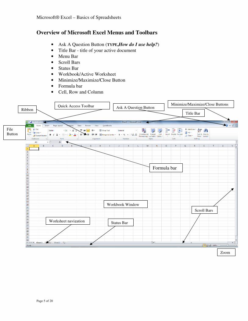
Overview of Microsoft Excel Menus and Toolbars

• Ask A Question Button (TYPE,How do I use help?)

• Title Bar - title of your active document

• Menu Bar

• Scroll Bars

• Status Bar

• Workbook/Active Worksheet

• Minimize/Maximize/Close Button

• Formula bar

• Cell, Row and Column

Title Bar

Scroll Bars

Minimize/Maximize/Close Buttons Ask A Question Button

Formula bar

Status Bar Worksheet navigation

Ribbon

Workbook Window

Quick Access Toolbar

File Button

Zoom

Microsoft® Excel – Basics of Spreadsheets

Page 6 of 20

Customize Toolbar/Commands and Options

To locate right click on the toolbar and select Customize Quick Access Toolbar…

Commands tab allows adding and removing items from the Quick Access Toolbar.

• In the list of optionsSELECTSet Print Area in the commands list,

andADD to Toolbar by clicking Add>>.

Options tab

• The Advanced Section has most of the previous commands that were found in the older Option Menus.

• The Popular Section has the ability to change the color and the ability to change the user name.

• The Proofing Section holds the location from the AutoCorrect options.

Customize Ribbon

• New in 2010 – we are now able to change the ribbon itself by adding or removing tabs or items

Things to remember:

Microsoft® Excel – Basics of Spreadsheets

Page 7 of 20

Insertion Point - The blinking, short, vertical line, it indicates where your next typing (or backspacing) will begin.

I-beam -The cursor shape (I) that controls the movement or placement of the Insertion Point controlled by the mouse.

Point -Move the pointer on a display screen to select an item. Click -To tap on a mouse button, pressing it down and then immediately releasing it (one press-

and-release of the mouse). Note that clicking a mouse button is different from pressing (or dragging) a mouse button, which implies that you hold the button down without releasing it. The phrase to click on, means to select (a screen object) by moving the mouse pointer to the object's position and clicking a mouse button.

Double-click - Tapping the mouse button twice in rapid succession. Note that the second click must immediately follow the first, without moving the mouse, otherwise the program will interpret them as two separate clicks rather than one Double-Click. (generally used to open an icon or select a single word)

Drag - Refers to any operation in which the mouse button is held down while the mouse is moved. Right click - access different shortcut menus, menus vary depending on where you are clicking. Left click - select button. Select / Deselect - highlighted or non-highlighted text.

Navigating through Excel

Soon after you install Office 2003 on your computer, a balloon pops up asking if you would like to "Help Make Office Better." If you click on it, you are given the opportunity to enroll in something called the Microsoft Office Customer Experience Improvement Program. If you opt-in, anonymous data about how you use Office are uploaded to Microsoft occasionally in the background. All of this data went back to the developers in Redmond on how you use your computer. This is what they found:

Top 5 Most-Used Commands in Microsoft Word 2003

1. Paste

2. Save

3. Copy

4. Undo

5. Bold

Together, these five commands account for around 32% of the total command use in Word 2003. Paste itself accounts for more than 11% of all commands used, and has more than twice as much usage as the #2 entry on the list, Save. With this information, the developers went out and created a new interface for Office 2007. This interface was then refined for Office 2010. The new Microsoft Office Fluent user interface primarily consists of nine key components:

Microsoft® Excel – Basics of Spreadsheets

Page 8 of 20

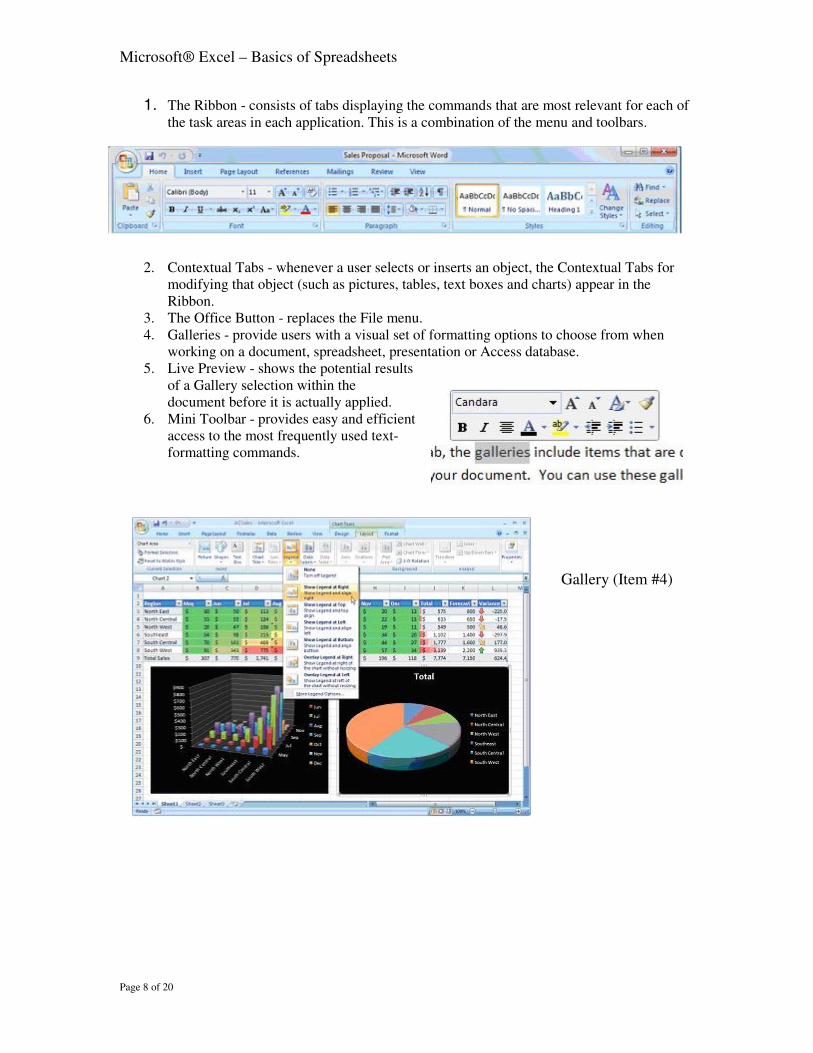
1. The Ribbon - consists of tabs displaying the commands that are most relevant for each of the task areas in each application. This is a combination of the menu and toolbars.

2. Contextual Tabs - whenever a user selects or inserts an object, the Contextual Tabs for

modifying that object (such as pictures, tables, text boxes and charts) appear in the Ribbon.

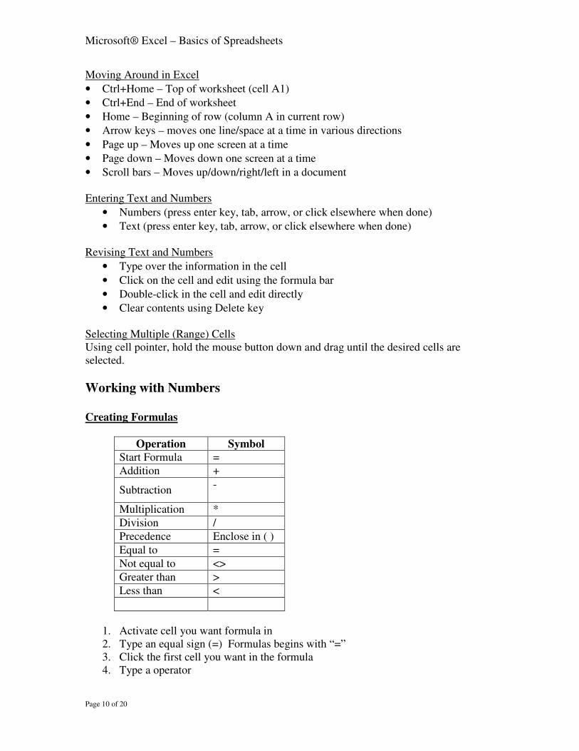
3. The Office Button - replaces the File menu. 4. Galleries - provide users with a visual set of formatting options to choose from when

working on a document, spreadsheet, presentation or Access database. 5. Live Preview - shows the potential results

of a Gallery selection within the document before it is actually applied.

6. Mini Toolbar - provides easy and efficient access to the most frequently used text-formatting commands.

Gallery (Item #4)

Microsoft® Excel – Basics of Spreadsheets

Page 9 of 20

7. Enhanced ScreenTips - appears as users move the mouse pointer over items in the Ribbon, showing the name of the feature, the keyboard shortcut and a brief description of what the feature is used for, and help links.

8. Quick Access Toolbar - provides a single location for people to place the commands and features they use most frequently.

9. KeyTips - appear in front of the Ribbon tabs with a single letter or combination of letters for users to type to activate the feature when users press the Alt key.

Time saving tip:

Right Mouse Button allows users to access menu items easier and faster.

Use Keyboard Shortcuts. (hold Ctrl key down and press the “assigned” key)

Use Toolbars instead of Menu items.

Understanding and Moving around in Excel Exercise One:

Enter in the information as below

Name Payrate Hours Gross Pay

Fredrickson 9.5 38

Jones 9 39

Monroe 10.25 37

Peterson 9 40

Smith 11.25 40

Workbooks are saved as files Worksheets is a page within the workbook

• Sheets can be inserted (Insert>Worksheet)

• Sheets can be renamed (Double click on sheet name and type in new name)

• Worksheet Components

Active Cell

Gridline

Row Heading

Column Heading

Fill Handle

Microsoft® Excel – Basics of Spreadsheets

Page 10 of 20

Moving Around in Excel

• Ctrl+Home – Top of worksheet (cell A1)

• Ctrl+End – End of worksheet

• Home – Beginning of row (column A in current row)

• Arrow keys – moves one line/space at a time in various directions

• Page up – Moves up one screen at a time

• Page down – Moves down one screen at a time

• Scroll bars – Moves up/down/right/left in a document Entering Text and Numbers

• Numbers (press enter key, tab, arrow, or click elsewhere when done)

• Text (press enter key, tab, arrow, or click elsewhere when done) Revising Text and Numbers

• Type over the information in the cell

• Click on the cell and edit using the formula bar

• Double-click in the cell and edit directly

• Clear contents using Delete key Selecting Multiple (Range) Cells Using cell pointer, hold the mouse button down and drag until the desired cells are selected.

Working with Numbers

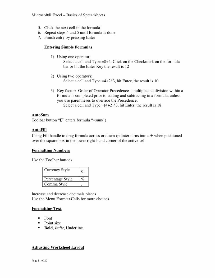
Creating Formulas

Operation Symbol

Start Formula =

Addition +

Subtraction -

Multiplication *

Division /

Precedence Enclose in ( )

Equal to =

Not equal to <>

Greater than >

Less than <

1. Activate cell you want formula in 2. Type an equal sign (=) Formulas begins with “=” 3. Click the first cell you want in the formula 4. Type a operator

Microsoft® Excel – Basics of Spreadsheets

Page 11 of 20

5. Click the next cell in the formula 6. Repeat steps 4 and 5 until formula is done 7. Finish entry by pressing Enter

Entering Simple Formulas

1) Using one operator:

Select a cell and Type =8+4, Click on the Checkmark on the formula bar or hit the Enter Key the result is 12

2) Using two operators: Select a cell and Type =4+2*3, hit Enter, the result is 10

3) Key factor: Order of Operator Precedence - multiple and division within a formula is completed prior to adding and subtracting in a formula, unless you use parentheses to override the Precedence.

Select a cell and Type =(4+2)*3, hit Enter, the result is 18 AutoSum

Toolbar button “ΣΣΣΣ” enters formula “=sum( ) AutoFill

Using Fill handle to drag formula across or down (pointer turns into a ++++ when positioned over the square box in the lower right-hand corner of the active cell Formatting Numbers

Use the Toolbar buttons

Currency Style $

Percentage Style %

Comma Style ,

Increase and decrease decimals places Use the Menu Format>Cells for more choices Formatting Text

� Font � Point size � Bold, Italic, Underline

Adjusting Worksheet Layout

Microsoft® Excel – Basics of Spreadsheets

Page 12 of 20

♦ Adjusting Column Width and Row Height � Adjust Column Width

• Select column you want to adjust (A, B, C, etc.)

• Place the mouse pointer to the right edge of the selected column until the pointer changes into a double-headed arrow

• Double click to have Excel adjust it to the best fit for that column, or hold the mouse button down and drag to the right or left until desired width is reached

� Adjust Row Height

• Select row you want to adjust (1, 2, 3 etc.)

• Place the mouse pointer to the lower edge of the selected row until the pointer changes into a double-headed arrow

• Double click to have Excel adjust it to the best fit for that row, or hold the mouse button down and drag up or down until desired height is reached

♦ Inserting and Deleting Rows and Columns � Insert Row or Column

• Right-mouse button click on Column or Row heading you want to move to the right or down, right-click and select Insert (select multiple columns or rows prior to this if you want to insert more at one time)

� Delete Row or Column

• Right-mouse button click on the Column or Row heading you want to delete and choose Delete from the menu

♦ Since the Employees are in alphabetical order, insert Peart at $11 and 40 hours above Peterson. Notice that the formatting is the same for the columns, but that you have to autofill the formulas that were put in to calculate gross pay.

♦ Inserting and Deleting Cells

♦ Moving and Copying Cell Contents � Using Copy and Paste commands

• Select range of cells and choose copy and then put insertion point in new spot and choose paste to duplicate

• Select range of cells and choose cut and then put insertion point in new spot and choose paste to move

� Using Drag and Drop function

• Select range of cells, move mouse to lower edge of range, when arrow appears, hold mouse down and drag and drop to new location to move

• Select range of cells, move mouse to lower edge of range, when arrow appears, hold Ctrl key down and mouse down and drag and drop to new location to copy

Microsoft® Excel – Basics of Spreadsheets

Page 13 of 20

Aligning Text

• Rotating Text

• Format > Cells > Alignment tab

• Or Select cells and right-click over selection

• Merge, Shrink to Fit, and Wrap Text

• Also listed under Format > Cells > Alignment tab

• Merge and Center

Borders and Color/Shading

• Borders

• Select range

• Right click and select Format

Cells…Select the Border tab on the Format Cells Screen

• Colors/Shading

• Select range you want to color or shade

• Right click and Use the mini toolbarand select the fill button and select the color to shade the cells.

Select range of cells and choose “Merge and Center” command from the Ribbon

Microsoft® Excel – Basics of Spreadsheets

Page 14 of 20

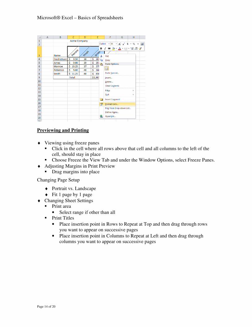
Previewing and Printing

♦ Viewing using freeze panes

� Click in the cell where all rows above that cell and all columns to the left of the cell, should stay in place

� Choose Freeze the View Tab and under the Window Options, select Freeze Panes.

♦ Adjusting Margins in Print Preview � Drag margins into place

Changing Page Setup

♦ Portrait vs. Landscape

♦ Fit 1 page by 1 page

♦ Changing Sheet Settings � Print area

• Select range if other than all � Print Titles

• Place insertion point in Rows to Repeat at Top and then drag through rows you want to appear on successive pages

• Place insertion point in Columns to Repeat at Left and then drag through columns you want to appear on successive pages

Microsoft® Excel – Basics of Spreadsheets

Page 15 of 20

Creating Easy-to-Understand Charts

♦ Understanding Chart Types � Column Charts

• Compares values across categories � Pie Charts

• Displays the contribution of each value to a total � Line Charts

• Displays trends over time or categories

♦ Creating a Chart � Using the Chart Wizard

• Select range to include text and numbers

• Select the Insert tab, and then the type of chart from the menu.

• Move through 4 steps until finished

Other Options with Excel

Microsoft® Excel – Basics of Spreadsheets

Page 16 of 20

Exercise Two:

1. If not already open, OPENa new Excel Workbook 2. To add a worksheet title, CLICKon cell B2, andTYPE2010 Cash Flow Summary,

thenPRESSEnter 3. To add labels for the columns of data, PRESSthe down arrow key, then

TYPEQuarter(this should be in cell B4) and PRESSEnter. 4. To enter labels for rows, CLICKcell B5 and TYPEQ. Note: Excel gives you the option

of completing the cell using the option of completing the cell using the same text as the entry above. TYPE1, then PRESS Enter.

5. Finish entering label rows. Currently, the selected cell should be B6. TYPEQ2. Using the mouse cursor, Pointto the fill handle on the bottom right corner of the selected cell. Note: the point becomes a cross. While holding down the left mouse button DRAGthe fill handle to cell B8. Note: Excel automatically fills in and increments the values in cells B7 and B8.

6. Using the mouse, select cell C4. TYPEFrance,PRESSRight Arrow key, TYPEGermany, PRESSRight Arrow key, TYPESpain, PRESSEnter.

7. To begin entering numeric values into the worksheet, CLICKcellC5,TYPE55000(no commas needed!), PRESSenter. Note: numbers right align by default. CLICKcell C6, TYPE175000, PRESSenter.

8. Complete the table inserting numbers as below.

2010 Cash Flow Summary

Quarter France Germany Spain

Q1 55000 300000 45000

Q2 175000 275000 25000

Q3 25000 125000 75000

Q4 145000 0 155000

9. CLICKin cellF4, TYPETotal, and PRESS Enter. To use the AutoSum

feature to sum the first row of data, CLICKthe AutoSum button on the Ribbon.PRESSEnter.

10. CLICKin cell F4again. Using the AutoFill handle in the lower right hand side of the selection, DRAG the cursor down to F9.Then CLICKin cell F9.

11. To get the totals for each country, CLICKin cellC9. Use the AutoSum feature to sum the first column of data in C9. PRESS Enterplace the function in that cell.

12. CLICKin cellC9 again. Using the AutoFill handle in the lower right hand side of the selection, DRAG the cursor down to F9. Then CLICKin cell F9.

13. Format all of the numbers as currency by selecting cells C5 through F9. CLICKin cellC5. While holding the left mouse button, DRAGthe cursor until cell F9 is reached.

All of the cells minus cell C5 should have a blue tint. 14. Name the sheet byDOUBLE-CLICKING on the Tab that shows Sheet 1. TYPE 2010

CASH FLOW and press ENTER.

Microsoft® Excel – Basics of Spreadsheets

Page 17 of 20

15. To copy the contents of 2010 Cash Flow to Sheet2, DRAGthe pointer down from cell B2 to F10on 2010 Cash Flow. RIGHT-CLICKthe selected cells and CLICK Copy. CLICKthe sheet2 tab. To paste the clipboard contents into sheet 2, CLICKB2, PRESSEnter.

16. To change the worksheet title text, DOUBLE-CLICK“2010” in the Formula Bar, TYPE2011, PRESSEnter.

17. Name this sheet byDOUBLE-CLICKING on the Tab that shows Sheet 2. TYPE 2011

CASH FLOW and press ENTER. 18. Follow steps 15 through 17 and copy Sheet 2011 Cash Flow to Sheet 3 and rename it

2012 CASH FLOW.

19. To add a fourth worksheet, CLICKon the tab with the Starburst to the far right of all the tabs.

20. To rename the new worksheet, DOUBLE-CLICKthe Sheet4 tab, TYPEThree Year

Totals, PRESSEnter. 21. SAVEfile.

Completed Exercise:

2012 Cash Flow Summary

Quarter France Germany Spain Total

Q1 $ 55,000.00 $ 300,000.00 $ 45,000.00 $ 400,000.00

Q2 $ 175,000.00 $ 275,000.00 $ 25,000.00 $ 475,000.00

Q3 $ 25,000.00 $ 125,000.00 $ 75,000.00 $ 225,000.00

Q4 $ 145,000.00 $ - $ 155,000.00 $ 300,000.00

$ 400,000.00 $ 700,000.00 $ 300,000.00 $ 1,400,000.00

Microsoft® Excel – Basics of Spreadsheets

Page 18 of 20

Time Saving Tips: Keyboard Navigation

There are many times when your worksheet fills more than a single window and it doesn’t take long before you want to find ways to move about the worksheet more quickly. The table below will provide you with some quick ways to travel through out your worksheet.

To Go Here Press this key combination Notes

Active cell Ctrl + Backspace Use this shortcut if the active cell has scrolled off the screen.

Next unlocked cell Tab

Previous unlocked cell Shift + Tab

Beginning of current row Home

Last column containing any filled cells in the current row

End, then Enter

Beginning of the worksheet Ctrl + Home

Last worksheet cell Ctrl + End Cell at intersection of last row and column used.

Up or down one screen Page Up or Page Down

Left or right one screen Alt + Page Up or Alt + Page Down

Next or previous worksheet Ctrl + Page Up or Ctrl + Page Down

Navigating to other worksheets

When you have more worksheets within your workbook that show without scrolling, you can right-click on the scrolling buttons to the left of the worksheet tabs and choose the destination sheet from the short cut menu. You will be able to see up to 15 sheets at one time

You can rename the sheets by doubling-clicking on the sheet tab name and then retyping in a new name. An alternative is to right-click on the sheet tab and select Rename from the shortcut menu.

Shift-Click Trick

Do you get frustrated when you are trying to select a range that exceeds the width or height of your screen (you end up scrolling over or down sometimes hundreds of rows or many columns before you can stop)? Try this trick next time. First, click in the top corner of the range you want to select. Next, using the scroll bars only, scroll down until you see the bottom of the range of the cells you want to select. Holding down the Shift key, click in the opposite corner from the cell you first selected. If the range isn’t exactly right, keep the Shift down while you re-click.

Making Multiple Selections

It is sometimes necessary to create a pie chart, for example, using information in cells that are not adjacent to each other as the figure below indicates. To select nonadjacent ranges, or cells, simple select the first cell or range you want in the normal fashion, then hold down the Ctrl key as you select the next cell or range, repeating until all required cells or ranges have been selected.

Microsoft® Excel – Basics of Spreadsheets

Page 19 of 20

In addition to using this method when you need to create a pie chart, you can also use it to select cells or ranges that aren’t next to each other and apply formatting to them.

Summing Up a Few Numbers

You can quickly sum up a few numbers (a range or using the method above to select nonadjacent cells) by selectinglooking for the “Sum” line on the status bar.

If you right-click any of those wordscan select other options.

Getting what you type

If you want to type in 1/2 in a cell, you will find that Excel thinks you

want the date, January 2the date.

Type in a 0 (zero) first followed by a space. This will display a 1/2, and the cell will display a .5 in the formula bar.

Adding a carriage return

To enter a hard carriage return in a cell, pwhere you want the line to break. This will turn on the Wrap Text Format and will automatically adjust the row height so the text will fit. You can find the Wrap Text Format under the Format Menu, on the Alignment Tab of the Cells Comm

Error Messages

When a cell with an error in the formulaERROR button appears next to it. You can click the buttons down arrow to display a menu with options that provide information about the error.

• #### - The column isn’t wi

Basics of Spreadsheets

33%

22%

Revenue by Rep

Dale Rita

In addition to using this method when you need to ie chart, you can also use it to select cells

or ranges that aren’t next to each other and apply

Summing Up a Few Numbers

You can quickly sum up a few numbers (a range or using the method above to select nonadjacent cells) by selecting them and looking for the “Sum” line on the status

any of those words, you can select other options.

If you want to type in 1/2 in a cell, you will find that Excel thinks you want the date, January 2nd. That is because the dash, “/”, is used to format for

ype in a 0 (zero) first followed by a space. This will display a 1/2, and display a .5 in the formula bar.

To enter a hard carriage return in a cell, press the Alt+Enter where you want the line to break. This will turn on the Wrap Text Format and will automatically adjust the row height so the text will fit. You can find the Wrap Text Format under the Format Menu, on the Alignment Tab of the Cells Command.

When a cell with an error in the formula is the active cell an button appears next to it. You can click the buttons down arrow to display a

menu with options that provide information about the error.

The column isn’t wide enough to display the value.

45%

Revenue by Rep

Rita Steven

You can quickly sum up a few numbers (a range or using the method above to select

If you want to type in 1/2 in a cell, you will find that Excel thinks you That is because the dash, “/”, is used to format for

ype in a 0 (zero) first followed by a space. This will display a 1/2, and

button appears next to it. You can click the buttons down arrow to display a

Microsoft® Excel – Basics of Spreadsheets

Page 20 of 20

• #VALUE! – The formula has the wrong type of argument. (such as when it is true or false)

• #NAME? – the formula contains text that Excel doesn’t recognize. (such as an unknown named range)

• #REF! – The formula refers to a cell that doesn’t exist. (which can happen whenever cells are deleted)

• #DIV/0! – The formula attempts to divide by zero.

Excel Shortcuts

Activity Shortcut Keys Alternate between displaying cell values and displaying cell formulas CTRL+` (single left

quotation mark)

Calculate all sheets in all open workbooks F9

Calculate the active worksheet SHIFT+F9

Copy CTRL+C

Create a chart that uses the current range F11 or ALT+F1

Display the FormatCells dialog box CTRL+1

Display the GoTo dialog box F5

Fill the selected cell range with the current entry CTRL+ENTER

Insert the current time CTRL+:

Insert today's date CTRL+;

Move to the beginning of the worksheet CTRL+HOME

Move to the last cell on the worksheet, which is the cell at the intersection of the rightmost used column and the bottommost used row (in the lower-right corner), or the cell opposite the home cell, which is typically A1

CTRL+END

Open CTRL+O

Paste CTRL+V

Paste a function into a formula SHIFT+F3

Print CTRL+P

Save CTRL+S

Select all (when you are not entering or editing a formula) CTRL+A

Select the current column CTRL+SPACEBAR

Select the current row SHIFT+SPACEBAR

Undo CTRL+Z

When you enter a formula, display the Formula Palette after you type a function name CTRL+A