Basics of SPSS

USING SPSS/PC+TO ANALYZE RESEARCH DATA:

A Step-by-Step Manual

Fourth Edition

by

Lars E. Perner

Robert H. Smith School of BusinessUniversity of Maryland

College Park, MD 20742-1815, U.S.A.Internet: [email protected]

http://www.rhsmith.umd.edu/~lperner

Copyright (C) 1989, 1990 by Lars E. Perner

i

Acknowledgements

The writer would like to thank Pat Stewart of Pennsylvania StateUniversity, Marie Rowland of the City of San Luis Obispo, California, andnumerous students enrolled in marketing research courses for their usefulfeedback on previous editions of this guide.

ii

Contents

Acknowledgements ..................................................................................................... ii

To the Instructor ........................................................................................................... v

To the Student .............................................................................................................. ix

What Can SPSS/PC+ Do for Me?............................................................................. 1

Introduction................................................................................................................... 9

Step 1: Coding Your Data......................................................................................... 11

Step 2: Writing An SPSS/PC+ Program.............................................................. 20

Step 3: Entering The Program And Data............................................................. 30Exercise 1 .......................................................................................................... 33

Step 4: Checking Your Data And Program For Errors ..................................... 35

Step 5: Using Statistical Procedures And Computations ................................ 38Frequencies ........................................................................................................ 38Creating New Variables: Compute.............................................................. 39Recoding Variables ........................................................................................ 39Crosstabulation............................................................................................... 41Product Moment (Pearson) Correlation .................................................... 45Multiple Linear Regression........................................................................... 47Discriminant Analysis .................................................................................. 48"""Count: "Counting" on how many variables a criterion is met ........ 49Descriptives: A summarized version of Frequencies ............................ 49Npar tests: Non-parametric statistical tests............................................ 50Means: Providing a breakdown of population means by

subgroup............................................................................................... 51Oneway and ANOVA: Analysis of Variance ........................................... 52Plot: Turning bivariate data into a scatterplot....................................... 52

iii

Reliability: Finding coefficient Alpha and other measures ofreliability in a scale ............................................................................ 54

t-test: Testing for differences in two population means. ..................... 55Advanced features: Factor, Cluster, Hiloglinear, and MANOVA........ 56

Appendices:

A: Common Questions About SPSS/PC+........................................................ 58 B: Working With SPSS/PC+ Output................................................................... 61

Frequencies ...................................................................................................... 61Crosstabs .......................................................................................................... 65Pearson Correlation....................................................................................... 68

C: Working With Large Data Sets....................................................................... 72 D: Using System Files ............................................................................................. 74 E: Importing Data From Lotus 123 ..................................................................... 77 F: Similarities Between SPSS/PC+ and Lotus 123........................................... 80 G: Similarities Between SPSS/PC+ and dBase III+......................................... 83 H: SPSS-X: The Mainframe Version................................................................... 85 I: Incorporating SPSS/PC+ Output Into WordPerfect Reports................... 86 J: Dealing With Printer Problems..........................................................................88 K: Statistical Significance...................................................................................... 89 L: Expanded Glossary...............................................................................................95 M: Additional Sources of Information............................................................. 110

iv

To the Instructor

This text is intended to meet the needs of students enrolled in a oneterm course which is only partially devoted to data analysis. In such asituation, the instructor cannot afford to take out a major part of the class todiscuss the theoretical aspects of data analysis and processing. In fact, thisbook resulted from the frustration I experienced in not being able to find atextbook suitable for a one quarter marketing research methods course ofwhich only the last three weeks were devoted to data analysis.

My emphasis has been on getting the student started on doing his orher own analysis as quickly as possible. Rather than discussing the conceptsand commands in a highly theoretical manner, I have presented some veryreadable and illustrative examples. A discussion of the concepts andmechanics behind these examples is intended to enable the student togeneralize these illustrations to their own projects.

I have taken several steps aimed at enhancing the student'sunderstanding of the analytical process. For example, I have chosen toconsistently place data in the same file as the SPSS/PC+ program and haveconfined any treatment of the topic of system files to an appendix. Whilethis may at first glance seem to be a wasteful approach which requires theuser to run the same program over and over, I believe it helps the studentmore clearly understand where the data comes from. For the samepedagogical reasons, only a fixed data format is used. Not only does a fixeddata column arrangement promote a better appreciation of how eachvariable is associated with every case; it also avoids inevitable sequencedisplacement problems that occur when the free format is used.

I have deliberately omitted discussion of the menu driven commandsystem and the optional data entry module. While some users find thesefeatures useful, I believe that a clearer understanding is reached by typing inone's own commands. The menus can't supply such information as thevariable and value labels, which account for the majority of the programanyway. What is more, once one gets into trouble with the menus, it is often

v

very difficult to get out. As for typing in the data directly, rather thanthrough the data entry module, it is my experience that such practice helpsthe user appreciate the fixed format of the data entry. Also, this method ofdata entry is more efficient for large data sets since the "key puncher" is notrequired to enter a carriage return after entering each variable.

These approaches, along with my avoidance of alphanumericvariables, further allow for a better generalization to other statisticalpackages and formats.

Students today are increasingly computer literate, and it is notunusual for students to be familiar with such software programs as Lotus123 and dBase. I have included appendices that illustrate similarities anddifferences between these programs in order to help students who alreadyknow the programs easily understand comparable procedures andoperations of SPSS/PC+. An appendix also indicates how data can beimported from such sources as Lotus 123.

The other side of the coin is that many people still feel uneasy when itcomes to dealing with computers. Many official software manuals, andeven a number of secondary texts, tend to present the material in arelatively abstract and "sterile" manner. At the loss of a slight degree ofgenerality, I have instead chosen to present examples that will help the user"fill in the blanks" on his or her own programs. That is, I frequently use"real" variable names rather than referring to some abstract notion such as"varlist." In addition, I have used a great deal of humor andanthropomorphism to put the "reluctant" computer user off guard. On thattopic, I see no reason why humorous examples cannot be as informative andeducational as boring ones. The purpose of examples is to show the studenthow data can be analyzed, and while "real World" projects may be lessengrossing, the skills learned in a humorous situation can be generalized to aroutine, or perhaps even boring, situation.

The ease with which computers can perform a large number ofcomputations within a few moments creates the potential for a great deal ofabuse. It is almost certain that something "significant" will show up if oneperforms enough tests. Thus, I have strongly emphasized the practice of

vi

making a limited number of hypotheses before running the statisticalprocedures. The program named "SIGNIF.EXE," which is included on thedistribution diskette for this manual, allows the user to compute theprobability of making at least one Type I error given n significance tests. Having noted students' tendency to attempt a very large number ofanalyses, it is strongly recommended that the instructor stress the concept ofaccumulating error levels in class.

Since this is intended as an introductory textbook, it only discussesthose statistical techniques that would likely be encountered in anintroductory course. However, as students complete this book and theexercises contained herein, they should be well prepared to consult theofficial manuals issued by SPSS, Inc. These manuals also provide anexcellent discussion of the theory behind the statistical procedures involved.

Whenever one attempts to write a textbook for even a mildly diversegroup of readers, the question of how much background should be assumedfrom the reader arises. In the present case, such a concern is particularlyrelevant when it comes to deciding how statistical output should beinterpreted. My choice, for better or for worse, has been to leave anyextensive discussion of the statistical principles involved to the instructorand/or any other textbooks and reference materials that may have beenmade available to the student. I have only touched lightly on such topics asstatistical significance, although examples and brief discussions of thetechniques available might suggest applications appropriate for specificstatistical procedures. In order to accommodate users with highly diversestatistical backgrounds, I have included, as an appendix, an expandedglossary that explains many of the terms that the student may findunfamiliar.

With SPSS being available in so many forms, one may wonder aboutthe wisdom about using the personal computer version as opposed tomainframe versions such as SPSS-X available on most campuses. After all,SPSS/PC+ may be installed only on a few computers on campus whilemainframe terminals are readily available to students, some of whom mayeven be able to dial up the university mainframe by modem from home. Ithink there are several reasons why the PC version is preferable. First, many

vii

students have already had experience on the IBM PC and thus need muchless introduction. Secondly, should the student wish to include part of theSPSS output directly in a report, taking it from the "SPSS.LIS" output file ismuch easier than downloading an output file from the mainframe. Finally,those students who will end up using SPSS on the job are much more likelyto find a SPSS/PC+ than the mainframe version in industry.

In that same vein, a question arises as to whether one should use thecomplete SPSS/PC+ program or SPSS/PC+ Studentware. While I feel thatusing the "real thing" will be a better preparation for practical industryapplications, I don't think that students who only have the Studenwareedition available will be seriously shortchanged in an introductory course.

viii

To the Student

Much has changed since I was first exposed to the Statistical Packagefor the Social Sciences (SPSS) in the early 1980s. As an industry standard,SPSS now exists in versions for many different computers. At the time,however, I was confined to a mainframe version which did not seem terriblyuser friendly.

I didn't find the textbook assigned to be appreciably more userfriendly than the program. After several chapters referring to such abstractterminology as a "field," we finally got to write some programs, but thecoverage was still rather abstract. I have chosen a different, and hopefullymore readable approach, to writing about SPSS/PC+.

Many textbooks take the approach of presenting the theory fullybefore providing any examples. I don't find that a good way to learn. Fewof us learned to talk by studying a dictionary. Most of us instead learned bylistening to others and then adapting the language to suit our own needs.

I have chosen a similar approach in writing this book. First, we willlook at some SPSS/PC+ programs and explore what they do. Looking atthese examples, we will discuss how you can generalize the techniquespresented to meet your own needs.

This book is an introduction to SPSS/PC+, and as such, it covers onlya fraction of the options available. If you go on to use SPSS/PC+extensively, you will probably find the official manuals published bySPSS/PC+ to be invaluable. Not only do these manuals provide a greatsource of reference for the SPSS/PC+ procedures; they also provide anexcellent and very readable discussion of the statistical techniques available.

I have included some relatively humorous examples in this text. Aside from my own exaggerated sense of humor (which has a tendency toget me into trouble on many occasions), I think a witty approach may helpto (1) motivate you to keep up with the reading, and (2) help those people

ix

who feel uncomfortable with computers to feel more at ease with thesubject. You should not feel guilty about enjoying the reading, however. While you may risk getting some dirty looks in the library if you laugh outloud, the examples, although often far fetched, illustrate real research issuesand are just informative as boring examples. Why shouldn't enlightenedpoodle breeders commission marketing research just like the manufacturersof laundry detergent? Those people who split their investment fundsbetween an inventory of poodles and a controlling interest in Proctor &Gamble will be just concerned about increasing levels of prejudice againstsmall dogs as about consumer trends toward buying generic householdproducts.

A few final cautions. The computer has today made it very easy toperform statistical calculations that could literally have taken a personmonths to perform in past decades. With this potential, however, comes anopportunity for serious abuse. This can take two forms. First, anyone can docomplex statistical calculations in SPSS/PC+, but the output may not be atall meaningful. In class, you may have discussed the distinction betweennominal, ordinal, interval, and ratio scales of measurement. However, thecomputer doesn't know where your data comes from and will gladly complywith your request to include nominal data in a procedure that reallyrequires interval, or even ratio, level data. Therefore, be sure youunderstand the assumptions behind a statistical technique before running it.

The second potential for abuse results from our ability toindiscriminately perform a great number of analyses at the same time. Intuitively, it makes sense that if we try long enough to find something thatis "very unlikely," we will. Suppose, for example, that you decide to make atelephone survey to find out the birthdays of the respondent and his or herspouse. You call up a thousand married people at random from the phone-book (i.e., you terminate the interview once you find out that someone is notmarried). You then find out that three couples have their birthdays on thesame date. Any great discovery? Well, in each trial (call), the chance of"success" is approximately 1/365=0.00273. Multiplying our one thousandtrials times that 0.273% chance, we would expect about 2.73 couples in oursample to have the same birthday. Similarly, if you perform fiftysignificance tests at an α=0.05 level of significance, you would expect 2.5

x

tests to come out significant by chance alone.

1

What Can SPSS/PC+ Do for Me?

SPSS/PC+ is an incredibly beautiful program. If you like computersoftware, you might think of SPSS/PC+ as being as beautiful as programslike WordPerfect and Lotus 123. Unless you are a real nature enthusiast,you will probably find SPSS/PC+ even more impressive than a beautifulriver or mountain range. SPSS/PC+ will probably compare favorably withthe grandest piece of literature or greatest work of art you have ever seen. And, depending on how humanistic you are, you may also find SPSS/PC+more beautiful than the one you love. It's not surprising if, at first, you findthis statement difficult to believe, so let's get right into the features ofSPSS/PC+. You be the judge! (This chapter is intended to show you thevariety of statistical procedures available within SPSS/PC+, and may coverstatistical methods that you have not yet studied. The purpose is only toshow you what is available, and consequently, the chapter is not intendedfor detailed study.)

At the most basic level, you might want to tabulate some data youhave collected in a survey or through other means. Later on in the book, wewill meet a dog breeder who is very interested in whether people own dogsor not and what kind they prefer. Suppose he has asked you to do a survey. After you have entered the data, you can ask SPSS/PC+ for a table thatindicates how many people gave each of the possible answers to a question:

DOGOWN Ownership of Dog

Valid Cum Value Label Value Frequency Percent Percent Percent

Yes 1 82 46.9 49.1 49.1No 2 82 46.9 49.1 98.2Not sure 3 3 1.7 1.8 100.0Missing 9 8 4.6 MISSING ------- ------- ------- TOTAL 175 100.0 100.0

Mode 1.000 Minimum 1.000 Maximum 3.000

For example, the SPSS/PC+ output indicates that eighty-two peopleclaimed to have a dog, eighty-two claimed not to have one, three people

2

were not sure if they owned a dog or not, and nine people supplied answersthat were not interpretable or supplied no answer at all; hence, theiranswers are "missing."

Although SPSS/PC+ does notprovide good graphics capabilitiesexcept in an optional graphics modulethat many institutions do not have,you can use a spreadsheet or graphicspackage like Lotus 123, Excel, orQuattro to create a graph to depict theresponses given. It might looksomething like this:1

OK, so this saved you some timeand provided an output that was somewhat neater and more organizedthan what you would have obtained if you had done the calculations byhand. Is that all we have to be excited about?

Of course not! We are just beginning. SPSS/PC+ allows us to domore involved things as well. For example, we might be interested inassessing the relationship between two or more variables. One popularfeature allowing us to do this is the "crosstabs" table. Let's suppose that youhave been hired by a major airline that wants to diversify into thehospitality industry at its destination sites, offering consumers an integratedvacation package. In order to establish the kinds of restaurants that willappeal most to vacationers at each location, the airline would like to know ifthere is any relationship between food preference and favorite vacationdestination. After consulting your marketing textbook, you decide to do acrosstabulation. You think that people who prefer the Orient would be morelikely to prefer Chinese food; those people who prefer Europe would like

1

There is no need to cut and paste! Lotus graphics ("*.pic" files) can beimported directly into WordPerfect 5.0 or 5.1.

3

Italian and French food; and those people preferring the Continental U.S.would prefer Western type food such as steaks, hamburgers, and fries. Youare not quite sure about those who prefer to visit Hawaii. SPSS/PC+ allowsyou to test your hypotheses:2

Crosstabulation: VACPREF Preferred vacation destination By FOODPREF Preferred dinner meal Count �Western �Italian �Chinese �French �Other �

FOODPREF�> Row Pct � � � � � � Row

Col Pct � 1 � 2 � 3 � 4 � 5 � Total

VACPREF ��

1 � 20 � 1 � 5 � 3 � 1 � 30

U.S. Mainland � 66.7 � 3.3 � 16.7 � 10.0 � 3.3 � 20.0

� 83.3 � 3.0 � 8.5 � 10.3 � 20.0 �

��

2 � 1 � 1 � 11 � 1 � 2 � 16

Orient � 6.3 � 6.3 � 68.8 � 6.3 � 12.5 � 10.7

� 4.2 � 3.0 � 18.6 � 3.4 � 40.0 �

��

3 � 2 � 27 � 4 � 22 � � 55

Europe � 3.6 � 49.1 � 7.3 � 40.0 � � 36.7

� 8.3 � 81.8 � 6.8 � 75.9 � �

��

4 � 1 � 4 � 39 � 3 � 2 � 49

Hawaii � 2.0 � 8.2 � 79.6 � 6.1 � 4.1 � 32.7

� 4.2 � 12.1 � 66.1 � 10.3 � 40.0 �

��

Column 24 33 59 29 5 150 Total 16.0 22.0 39.3 19.3 3.3 100.0

Chi-Square D.F. Significance Min E.F. Cells with E.F.< 5 ---------- ---- ------------ -------- ------------------

156.76735 12 .0000 .533 8 OF 20 ( 40.0%)

Statistic Value Significance --------- ----- ------------

Cramer's V .59023-------------------------------------------------------------------------------

If you are familiar with the Chi square statistic, you can see that thereis strong evidence to reject the null hypothesis that food and vacationpreference are "independent." As a matter of fact, the Cramer's V statistic

2Normally, you should define hypotheses more specifically before

testing them. For now, we are just testing whether the two variables inquestion (food preference and favorite vacation destination) aredependent.

4

even suggests a modest relationship.

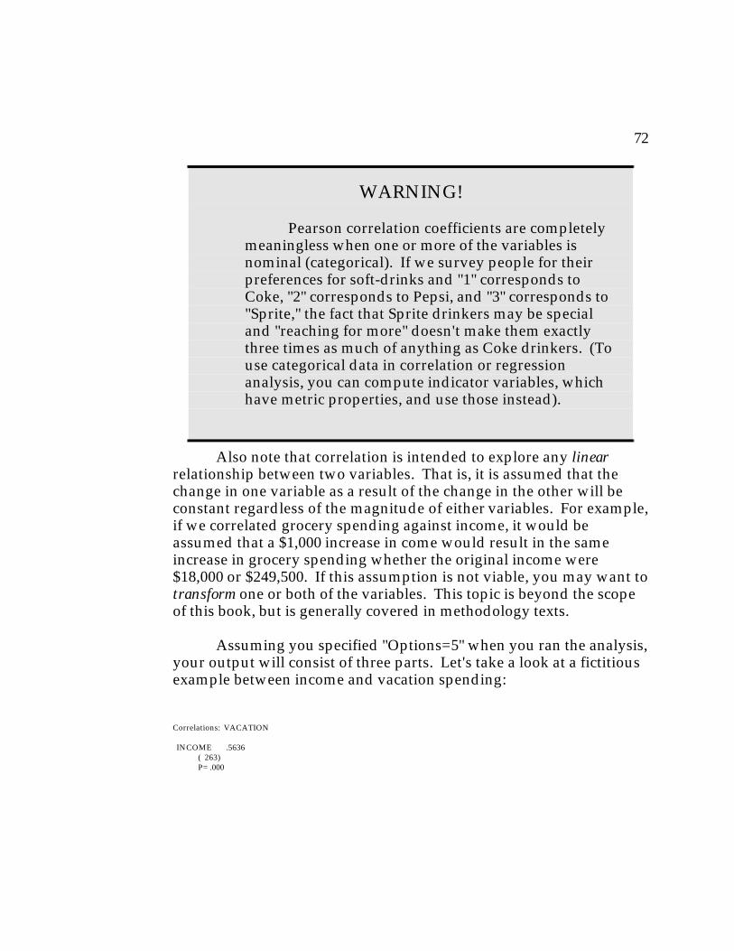
But, you are of course not limited to non-parametric statistics, orprocedures that only use ordinal measures, in SPSS/PC+. You can also do aPearson correlation analysis if you have interval data or "better."3 Let'ssuppose that the airline is interested in tourist travel and would like you toconduct a study of how to best predict how much money a person spends onvacation(s) every year. You decide to correlate amount spent on vacationsagainst various other variables.

Correlations: FOOD AUTO ENTERT DINING PHONE

VACATION .4304 .5754 .5728 .5620 .3498 ( 263) ( 263) ( 263) ( 263) ( 263) P= .000 P= .000 P= .000 P= .000 P= .000

Once you have done a correlation analysis, you might feel that theproper next step is to do a multiple regression analysis to see if you canimprove your ability to predict based on the introduction of additionalvariables. Unlike Lotus 123, SPSS/PC+ gives you several choices as towhich method you want to use (forward inclusion, backward deletion,stepwise consideration, or "forced" entry). If a traditional method doesn'tsuit your needs, you can introduce non-linear or log-linear models. Let's tryto "predict" a person's telephone bill from his or her expenditures on otheritems and other demographic information.

3

Actually, a correlation analysis is in practice applied many timeseven when only ordinal level data is available. This is not sanctioned ascorrect by most statisticians, but the this approach can sometimes stillyield meaningful results. When one or both of the variables departseriously from the assumption of interval properties, the true relationshipbetween the variables may be greatly underestimated. On the other hand,a correlation will rarely provide "false positives" or suggest a relationshipthat does not exist.

5

Variable(s) Entered on Step Number 3.. COMPUTER ownership of computer

Multiple R .67310R Square .45306Adjusted R Square .44673Standard Error 84.09635

Analysis of Variance DF Sum of Squares Mean SquareRegression 3 1517312.98023 505770.99341Residual 259 1831698.85247 7072.19634

F = 71.51541 Signif F = .0000

Equation Number 1 Dependent Variable.. PHONE total household phone bill

------------------ Variables in the Equation ------------------

Variable B SE B Beta T Sig T

DINING .09375 .01064 .58737 8.811 .0000AUTO .22249 .10231 .14281 2.175 .0306COMPUTER -36.34246 16.83655 -.10385 -2.159 .0318(Constant) 408.56124 31.01232 13.174 .0000

------------- Variables not in the Equation -------------

Variable Beta In Partial Min Toler T Sig T

FOOD -.05499 -.07431 .47474 -1.197 .2324ENTERT .02691 .01453 .13203 .233 .8156HOME -.02361 -.02499 .36798 -.401 .6884VCR -.02899 -.03802 .45710 -.611 .5417

End Block Number 1 PIN = .050 Limits reached.

-----------------------------------------------------------------

Not all statistical analyses have to be this involved. Maybe by nowyou are getting tired of doing research for someone else. Suppose that, forsome reason, you have a good cause to believe that there is a killing to bemade in retailing tall people's clothing. Not having a preference for eithermen's or women's clothing, but realizing that you need to specialize tocompete, you toss a coin and end up in the women's apparel business. Naturally, you will want to find a geographic location where there are a lotof tall women. Since you can't afford to research the heights of women allover the nation, you decide to focus on Texas in the belief that Texas citieswill be the most likely spots for success. You now proceed to collect data onthe heights of adult women (in inches) in Dallas and Houston. One way to

6

test for such differences would be to employ a t-test (two-tailed since youhave no preconceptions), but a more direct way might be to "break down"information by city. Using the SPSS/PC+ procedure Means you get thefollowing result:

Summaries of HEIGHT Height of subject (inches) By levels of CITY City of residence

Variable Value Label Mean Std Dev Cases

For Entire Population 66.6960 1.7183 200

CITY 1 Dallas 68.1830 .9038 100CITY 2 Houston 65.2090 .8069 100

Total Cases = 230Missing Cases = 30 OR 13.0 PCT.

Now you can optionally calculate a confidence interval for the meansof heights of the women on in each. Tentatively, it looks like Dallas might bethe best bet. (An added benefit is that by choosing this location, you will becloser to the Oil Barons' Club).

Of course, there is always the possibility that you decided to split thecost of doing the survey with a classmate who believes that there is moremoney to be made in tall men's clothing. In that case, of course, you wouldwant to find out about the heights of the men in the different cities as well. However, you would want to keep track of the heights of the men andwomen separately, both because the city that has the tallest men might nothave the tallest women and because the great between-sex heightdifferences would greatly inflate the estimate of within-gender variability. "Means" allows you to produce this table:

7

Summaries of HEIGHT Height of subject By levels of CITY City of residence SEX Sex of respondent Variable Value Label Mean Std Dev Cases

For Entire Population 68.9820 2.9810 200 CITY 1 Dallas 70.6840 2.6261 100 SEX 1 Male 73.1160 .8728 50 SEX 2 Female 68.2520 1.0492 50 CITY 2 Houston 67.2800 2.2614 100 SEX 1 Male 69.3700 .8929 50 SEX 2 Female 65.1900 .7875 50

Total Cases = 230Missing Cases = 30 OR 13.0 PCT.

Now that you have been working with SPSS/PC+ for quite some time,you are really getting good at marketing research, and you feel that you canhandle almost anything--even the unexpected. One day, you receive adistressed phone call from Rudolph the Redneck Reindeer. Rudolph ishysterical because his employer, an elderly man who likes to wear a red suitduring the winter months, has warned his long time sleigh puller that hemay have to lay him off because people are beginning to demand greatersophistication from reindeer. You agree to do a survey for Rudolph to findout how important that aspect really is to consumers. However, havingstudied marketing research for some time, you realize that one question or"item" will not give you a result that is reliable enough to give you an answerthat is dependable. You therefore decide to create a scale of "Appreciation ofSophistication in Reindeer," where subjects will be asked to indicate theirlevel of agreement or disagreement with Likert type questions on a scaleranging from "strongly agree" (1) "to neither agree nor disagree" (4) "tostrongly disagree" (7). Now you want to test whether the average score onthe questions will be reliable enough to be meaningful. You and Rudolphhope that people will score as low as possible on that scale, suggesting thathis employer's concern is unwarranted. After you "reverse score" item #4(which is worded in the opposite direction of the other questions), you areready to generate the following estimate of internal consistency:

8

R E L I A B I L I T Y A N A L Y S I S - S C A L E (S O P H I S T)

1. SOPHIS1 Good reindeer are educated 2. SOPHIS2 Reindeer should have good manners 3. SOPHIS3 A reindeer should have a good cultural background 4. SOPHIS4 Redneck reindeer are OK(Reverse scored) 5. SOPHIS5 Reindeer should use good grammar 6. SOPHIS6 Reindeer should be graceful 7. SOPHIS7 A reindeer's style is more important than the color of his nose

RELIABILITY COEFFICIENTS

N OF CASES = 100.0 N OF ITEMS = 7

ALPHA = .9218

Assessing internal consistency is an advanced topic, and you may notappreciate this capability yet, but the time will come! Please be patient untilthe end of the quarter.

SPSS/PC+ allows you to do many other beautiful things such asdiscriminant analysis, one-way analysis of variance, multivariate analysis ofvariance, factor analysis, cluster analysis, and various non-parametricstatistics. However, by now you ought to have seen enough to make aninformed judgment.

What's your verdict? I think you will agree that SPSS/PC+ is asbeautiful as WordPerfect and various other software programs. At least it ismore beautiful than a bouquet of roses or a beautiful waterfall. Now, howdoes it compare to that special person?

9

Introduction

Today, the data analysis involved in a marketing research project ofany real size is almost universally done by computer. Most statisticalprocedures involve a great number of arithmetic calculations which are notreally "difficult" to do by hand, but require a tremendous amount ofrepetitious work. Not only is this work boring and time consuming, but italso provides a great deal of opportunities for little mistakes which canseriously distort your actual results.

Today, many statistical software packages are available to help theresearcher avoid the repetitious work involved in number crunching. Notonly does such software allow us to save time, but the programs will alsoallow one to do analyses which simply wouldn't have been practical toperform in past years. While a researcher normally can't afford to literallyspend four weeks doing the calculations involved in a regression analysis oftwo hundred subjects with, say, ten independent variables, the computerwill do this analysis for him or her in seconds--that is, once the data set hasbeen entered, or typed, into the computer.

Although the micro computer version of the Statistical Package forthe Social Sciences (SPSS/PC+) is one of the leading statistical softwarepackages on the market, it is by no means the only useful one available. Thegroup of other powerful statistical packages includes the mainframe version(SPSS-X and SPSS v. 9.0) and such programs as the Statistical AnalysisSystem (SAS--available in both micro and mainframe versions) and theBiomedical Statistical Package (BMDP). Generally, you will find that theskills you learn while using SPSS can easily be transferred to these othersoftware with minor only modifications. Other programs, such as Minitab,are slightly easier to learn but not nearly as powerful and flexible.

SPSS has many features, of which you will probably only be using afew. It is important not to lose sight of the forest for the trees (or, in moremodern terms, not to lose sight of the computer for the chips). This manualcontains descriptions of many simple procedures to run, with moreinformation being available in various manuals put out by SPSS, Inc. and

10

third party sources. (If you are unsure about particular statisticalprocedures, these manuals also function very well as statistical texts sincethey contain very good, real life illustrations of the statistical techniquesdiscussed). The attempt of this book is not to teach you all the details ofSPSS/PC+, but simply to allow you to adapt sample programs to your needs.

Please don't be intimidated by the reference to "programming" withinSPSS/PC+. All this involves is putting together a few instructions for thecomputer telling it information about your data and how you would like toanalyze it. As a reasonably "user friendly" program, SPSS/PC+ acceptsrelatively "English-like" commands that make a great deal of sense eventhose people who don't spend most of their lives reading computer booksand magazines. Questions that SPSS/PC+ would like to have answeredrelate to issues such as:

• How many variables are in the data? • What do the different values mean? • What happens if a person didn't answer a question?

Considering the amount of time SPSS/PC+ saves us in doing thecalculations, I think it is fair enough that SPSS/PC+ expects to get that kindof information from us as a sort of "retainer." (In any event, it is not worththe effort to try to bargain with SPSS/PC+ since we need it more than itneeds us).

As we go through the writing of a program for a hypotheticalquestionnaire, you will be able to modify the statements of information forthat program to write one that fits your data.

11

Step 1: Coding Your Data

Assuming that you have already collected your data, the statisticalanalysis generally involves five stages:

1. Data coding, variable naming, and classification;2. Statistical program writing;3. Data Entry;4. Error checking; and5. Data analysis

We will go through each stage separately. In this chapter, we willdiscuss data coding.

In Figure 1-1, you will find a sample questionnaire, commissioned bya poodle breeder concerned about possible increasing prejudice againstsmall dogs, for which we will code and write an SPSS/PC+ program. Pleaseunderstand that this is not supposed to be an example of a goodquestionnaire. As a matter of fact, if you plan to use one like it in yourmarketing class, you should probably be prepared for a relatively low grade. The purpose of the questionnaire, instead, is to demonstrate how to code anumber of different questions. Later in this book, we will get to the touchingstory of the poodle breeder who has hired you to do a study of, among otherthings, prejudice against poodles.

12

DOG PREFERENCE QUESTIONNAIREWe are interested in your opinion about dogs and dog care. Please take a few minutes torespond to the questions below.

1. Do you own a dog? ___Yes ___No ___Not sure (If no, please skip to question 6)

2. How many dogs do you own? _______

3. What is the breed of your favorite dog? _____

4. Please rank the following foods in the order you prefer to feed them to your dog:

___ generic dry dog food ___ Lucky Dog food___ generic canned dog food ___ Kit 'n' Caboodle ___ Mighty Dog

5. How much do you spend on feeding your dog per week? $_______

6. Please write next to each of the questions below the number from the followingscale which most closely matches your level of agreement or disagreement:

1 2 3 4 5 6 7

Strongly Strongly agree disagree

___ 1. Poodles are fragile___ 2. Poodles are stupid___ 3. Poodles are self-centered___ 4. Poodles are cute___ 5. Poodles are over-priced

7. Age:____ Sex (Please circle): Male Female

Annual household income: $_____________

1Figure 1: The Poodle Breeder's Questionnaire

13

Whenever you plan to enter the contents of several questionnairesinto the computer, it is always a good habit to number each questionnaire. Let's do that in the top right corner.

The need to number the questionnaires introduces an important datacoding concept. Since we will ultimately be entering the data as numbers onone or more lines of text, we will want to determine the maximum numberof digits that a variable may take up. Suppose we administered threehundred questionnaires and numbered them, starting with one. In order tobe able to express all these ID numbers, we would need a minimum of threedigits for the ID field (since the numbers between 100 and 300 each take upthree digits. For a questionnaire administered to less than one hundredpeople, we would only need two digits for the ID.) If we assume that wehave three hundred surveys, we will eventually enter the ID number thisway:

001002003.. -------> more data here <--------..300

It is, of course, acceptable to allocate more digits than needed to avariable.

Now we get to actually code the questions. This includes giving thequestion (or variable) a one word name, assigning a number to each possibleanswer on the questionnaire4, determining how many digits are needed forthe question, determining in which columns the data will be put and,

4

SPSS/PC+ actually allows the use of alphanumeric characters, that is,letters of the alphabet, as data. However, the use of alphanumeric datawill often cause problems which are difficult to solve and it may be apoor practice since many other statistical programs will not allow suchdata.

14

optionally, assigning the question and answers "labels," i.e. short phrasesdescribing their meaning. Although this process may sound overwhelming,it is quite simple once we go through it.

The name of the variable can simply refer to the number of thequestion (e.g. "Q1," "ITEM18"), or it can be descriptive of the meaning of thevariable (e.g. "AGE," "INCOME.") The rules for naming SPSS/PC+ variablesare very similar to those for naming DOS files, i.e

• A variable must begin with a letter of the alphabet (unlike DOS, anumber is not acceptable) and may be up to eight characters long

• there may be no spaces in the name (thus, we say "ITEM1" and not"ITEM 1").

• A variable name may not be the same as certain "reserved" words, i.e.words that SPSS/PC+ uses for internal and programming purposes. These reserved words are very few and far between, but you cannotname your variables "AND," "OR," or "IF" as well as a few otherobscure names.

• SPSS/PC+ does not distinguish between upper and lower case letters. "QUEST1," "Quest1," and "quest1" all refer to the same variable andcan be used interchangeably.

• Unlike DOS file names, a variable name cannot have an extension.

The following variable names are valid:

Q1QUEST1QUEST1AQUESTA1

However, the following names are not acceptable:

1st Starts with a numberQuest 1 Contains a spaceMarketshare Consists of more than eight characters1st question Violates all of the above

15

Let's look at question number 1. Our first task is to name it. Eitheryou can call it something like Q1, to keep it simple, or you can name itsomething more descriptive like "DOGOWN." When you write your ownprogram, you have a choice; for now, we will call it DOGOWN. Next, noticethat there are three possible answers. (Your client insisted on including the"Not sure" option since the questionnaire would be administered in theneighborhood of a major university, making it likely that a number of absentminded professors would be asked to respond.) We now have to assign anumber to each. Let's assign a "1" to "Yes," a "2" to "No," and a "3" to "Notsure." Now, are these response categories enough?

Not really. Two things could happen. First, the respondent mightaccidentally overlook or refuse to answer the question (a common situationwhen you ask about such emotionally charged and private topics as incomeor extra marital activities). The next several questions illustrate thesituation that occurs when not everybody is supposed to answer a question,and we will discuss how to code such instances when we talk about thosequestions. For this question, missing data can only arise when a personeither omits the question or provides one that is not useful. This couldhappen if someone wrote a sarcastic comment instead of answering orsimply overlooked the question. Whenever a person fails to answer aquestion that he or she should have answered, we will assign a numeric value. For this question we will code it as a "9." When the question is notapplicable, just leave the space blank and the computer will assign theresponse as a "system missing value." (Notice that using "9" as the missingvalue for this question will result in all the numbers in between four andeight, inclusive, not being used).

The next question, which we will call DOGCOUNT, asks how manydogs the respondent owns. We will assume that the respondents arereasonably normal and do not own more than 98 dogs; hence, we willreserve only two digits for that variable. Note that here we may encounterthe kind of missing data that occurs when people legitimately omitquestions since the questions between sections two and five should only beanswered by those people who own dogs. When people "legitimately" skipquestions, we will put blank spaces in the columns designated for the

16

variable. For those people who indicated that they own at least one dog byanswering "Yes" to the first question but failed to answer this question, wewill put in the missing value of "99."

The third question, which we will call FAVORITE, is somewhat morecomplicated. This is what is called an "open ended" question; in otherwords, the subject is asked to write an answer and is not given a list of"acceptable" answers from which to choose. Therefore, we have to try tomatch each written answer with some kind of code that is general enough tobe meaningful. Since more than nine breeds are likely to be mentioned, wewill reserve two digits for this question. Notice that in order to occupy twocolumns, the numbers zero through nine must either be preceded by a blankor a zero. Thus, "01" might be "Poodle;" 02, "Fox Terrier;" 03, "YorkshireTerrier;" and so forth. Other options such as "10" as "German Shepherd" arepossible. (Several other breeds are listed in the program that we will get to). Again, a correctly omitted answer will result in two blank spaces and othercases of missing data will result in a code of "99."

Note that open ended questions have a great potential for missingdata. Suppose that someone misunderstood the question and thought he orshe was asked about his or her favorite pet. If he or she answered "Polarbear," you would most likely classify the answer as missing. You should beprepared for certain other kinds of "missing answers." Perhaps a respondentunsympathetic to the objectives of our research might scribble in somethinglike "I hate all dogs!"

To keep organized, we might consider giving very small dogs lownumbers, say, below 29; medium sized dogs intermediate numbers between30 and 59, and big dogs the bigger numbers between 60 and 98. Dependingon our research objective, we might also like to "cluster" the numbers on thebasis of other variables such as price, friendliness/viciousness, durability,guarding ability, or lifespan. Or, if we cared about none of those issues, wecould simply list the dogs in alphabetical order.

The next questions require very little discussion since subjects will beresponding directly with numbers. Thus, for section 4, all we have to do is toassign one digit to each variable (i.e. each dog food that we ask the

17

respondent to rate) and reserve "9" as a missing value. Skipping slightlyahead, the same holds for the Likert scale questions of Section 6.

In section 5, we will assume that no one spends more than $99.98 perweek on dog costs, and we will thus assign five digits and a missing value of"99.99." (SPSS/PC+ allows you to designate a variable as a dollar amountrather than as plain number. However, not all programs have thatcapability, so let's not get into that.) Also notice that we have are reservingspace for the period. We could arrange to use four digits instead, but why beso stingy with the space?

For age, we will assign two digits and a missing value of "99." For sex,"male" will be assigned "1" and "female" "2."

For the question of annual household income, we will assume that thefigure does not exceed 999,9985 for any respondent since we are located in auniversity community. We will thus reserve six digits since SPSS/PC+would not appreciate the comma (unlike the period allowed in the questionon weekly spending). Incidentally, anyone earning over a million dollars ayear would, in statistical jargon, probably be considered an "outlier"--a sortof maverick who would probably be excluded from our analysis anyway.

The table below summarizes the lengths, missing value indicators,and column positions of each variable. A "case," or collection of answersfrom one respondent (who owns a dog), could thus look like this:

001 1 02 02 52314 03.50 66727 29 2 026000

while a case from a person who does not own a dog, and thus was not askedto answer some of the questions, could look like this:

002 2 22252 31 1 032150

5

Remember, we need $999,999 (i.e. 999999) for missing data.

18

Variable MissingValue

Length Columns Label

________________________________________________________________________________IDOWNDOGDOGCOUNTFAVORITEFOOD1FOOD2FOOD3FOOD4FOOD5SPENDLIKERT1LIKERT2LIKERT3LIKERT4LIKERT5AGESEXINCOME

None 9 99 99 9 9 9 9 9 99.99 9 9 9 9 9 99 9999999

3 1 2 2 1 1 1 1 1 5 1 1 1 1 1 2 1 6

1- 3 5 7- 810-11 13 14 15 16 1719-23 25 26 27 28 2931-32 3437-42

Identification numberOwnership of dogNumber of dogs ownedBreed of favorite dogRanking of generic dryRanking of generic cannedRanking of Mighty DogRanking of Lucky DogRanking of Kit 'n'CaboodleWeekly expense of dog foodPoodles are fragilePoodles are stupidPoodles are self-centeredPoodles are cutePoodles are over-pricedAgeSexAnnual household income

A look at the column assignments and the two example cases

will show that we have put spaces between some variables and notbetween others. SPSS/PC+ leaves it entirely up to us whether wewant to leave such spaces or not. One of the first commands of theprogram simply tells it the column positions of each variable. Thus,we can to put spaces where they improve our ability to type in and read thedata.

For each case, a variable will be in the same column position(s). This can be a great help to ensure that we are on target when we typein the data. Consider, for example, the following two cases:

003 1 02 02 52314 03.50 66727 29 2 026000004 1 01 03 32512 05.50 67615 21 2 018500

Not only do we know that each case should end in the samecolumn; we also know that many of the blank spaces should be in thesame places. In this case, we have reserved blank spaces betweenmost of the variables, but none within the variables in the Likert scaleand rank-order sections. Putting in spaces there would make the dataseem more confusing.

19

How many persons over the age of 55 currently live in yourhousehold? __ a. None __ b. One __ c. Two __ d. Three __ e. Four or more

You should try to be as consistent as possible when codingdifferent questions within the same questionnaire. If for one questionyou use the code "1" for yes and "2" for no, you should try to keep thatpractice throughout the questionnaire.

When several people enter data, be sure that everyoneunderstands and agrees upon a coding system. There are numerousways the same variable can be coded. The variable SEX above, forexample, could have the codes "1" for male and "2" for female (as wedid); "1" for female and "2" for male; and "0" for female and "1" formale. None is inherently better or more correct than the other(although the first one is the most commonly used approach), but ifseveral individuals use different codes in the same file, a big editingjob could result.

Sometimes, the best way to code a variable does not coincidewith the coding that may be "suggested" by the questionnaire. Consider this example:

In this case, it might be tempting to start off at the beginningand number the choices from 1 through 5. This, however, would be abad approach, since the code "2" would now correspond to the answer"one person." Instead, you would be better off starting with zero andadvancing. That way, the code will correspond to the number of

20

people actually in the household.

21

Step 2: Writing An SPSS/PC+ Program

Now we are ready to pursue the bottom line of this text, that is,the writing of the SPSS/PC+ program. The next chapter will discusshow to enter the data and commands into SPSS/PC+; here, we willjust talk about what to enter. Here is a program for the questionnairewe have been discussing. Please don't be intimidated if it looksoverwhelming at first. We will go through it line by line.

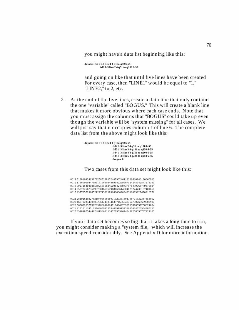
TITLE "Dog Preference Study".DATA LIST /id 1 -3 owndog 5 dogcount 7-8 favorite 10-11 food1 to food5 13-17 spend 19-23 (2) likert1 to likert5 25-29 age 31-32 sex 34 income 37-42.VARIABLE LABELS owndog "Ownership of dog" dogcount "Number of dogs owned" favorite "Breed of favorite dog" food1 "Rating of generic dry dog food" food2 "Rating of generic canned dog food" food3 "Rating of Mighty Dog" food4 "Rating of Lucky Dog" food5 "Rating of Kit 'n' Caboodle" spend "Weekly spending on dog food" likert1 "Poodles are fragile" likert2 "Poodles are stupid" likert3 "Poodles are self-centered" likert4 "Poodles are cute" likert5 "Poodles are over -priced" income "Annual household income".VALUE LABELS owndog 1 "Yes" 2 "No" 3 "Not sure"/ favorite 1 "Poodle" 2 "Fox Terrier" 3 "Yorkshire Terrier" 4 "Daschund" 10 "German Shepherd" 11 "Collie" 12 "Saint Bernard" 13 "Pit Bull" 14 "Malamute" 15 "Afghan" 16 "Cocker Spaniel" 17 "Dobermand" 18 "Golden Retriever" 19 "Rotweiler"/ food1 to food5 1 "Generic dry dog food" 2 "Generic dry cat food" 3 "Generic canned dog food" 4 "Kit 'n' Caboodle" 5 "Mighty Dog"/ sex 1 "Male" 2 "Female"/ likert1 to likert5 1 "Strongly agree" 7 "Strongly disagree".MISSING VALUE owndog likert1 to likert5 (9)/ dogcount favorite age (99)/spend (99.99)/income 999999.BEGIN DATA.001 1 02 02 52314 03.50 66727 29 2 026000002 2 22252 31 1 032150003 2 45445 26 2 135000004 1 01 03 32512 05.50 67615 21 2 018500

---> MORE DATA HERE <-----

999 2 77627 45 2 053000END DATA.FREQUENCIES VARIABLES=owndog to income/STATISTICS=all.

22

On The Use of Capitals

Unlike an English teacher, SPSS/PC+ doesn'tcare if you use upper or lower case letters. Thus, youcan mix and match as you find it convenient.

Let's take a look at what the lines in this program look like. Theprogram consists of several commands which are intended to instructthe computer about the data and what to do with it.

First, note that some lines are indented while others are not. Ingeneral, indented lines are continuations of commands were thatstarted immediately at the left margin on some line above it. SPSS/PC+ really doesn't care if you indent or not, but it will makeyour program more readable. As you can see, each commandeventually ends with a period, which tells the computer to take in thenext line as a new command. If you leave out the period, thecomputer will not understand your commands and will give you anerror message. Fortunately, such errors are easy to detect and correct,so if you leave out a few periods, it only means that you will have todo some editing after you first try to run the program. Evenexperienced SPSS/PC+ users often have problems in their firstattempts at any program, but the more experience you get with theprogram, the easier it gets to correct the problems.

Now, let's start from the beginning.

TITLE "Dog Preference Study".

This first command is actually optional. Eventually, SPSS/PC+will give pages of output consisting of statistical computations, andputting in the "title" command will put some heading that you chooseon top of every page. In terms of syntax, the word "title" is followedby the title you wish to assign in quotes. Notice that the period,contrary to what your junior high school English teacher taught you,goes outside the quotes.

23

DATA LIST /id 1-3 owndog 5 dogcount 7-8 favorite 10-11 food1 to food5 13-17 spend 19-23 (2) likert1 to likert5 25-29 age 31-32 sex 34

income 37-42.

This command is the most crucial part of the program. It mayalso be the one that can cause you the most frustration.

The "data list" command tells the computer about the positionsof the variables on the data lines. If you have made a table detailingthis information, you already have all the information needed. Otherwise, you will have to do some arithmetic now to calculate thebeginning and ending columns of each variable.

After typing in the command "data list," we will type in a slashto indicate that we are starting the definition of a line of data. Thecommand will not be recognized if you leave this slash out. Afterthat, we will list each variable followed by the column(s) it represents. Thus, we state that ID covers the columns one through three:

DATA LIST /id 1-3...

The variable OWNDOG only takes up one column, so no dash isneeded to indicate a range.

For a long questionnaire, we don't quite have to type in theinformation for each variable individually. Notice that we are able toconsolidate the information for the Likert scale section into onedeclaration:

likert1 to likert5 25-29

Since each variable takes up the same number of columns (inthis case one), SPSS/PC+ will recognize that the above declaration isidentical to the following more elaborate statement:

likert1 25 likert2 26 likert3 27 likert4 28 likert5 29

24

This statement only works because each variable takes up the samenumber of columns. If some of the listed variables took up two columnsand some just one, SPSS/PC+ would not have enough information todetermine how much each one got.

We have alluded to the fact that SPSS/PC+ knows that

item1 to item6

is the same as

item1 item2 item3 item4 item5 item6 .

However, SPSS/PC+ does not allow you to create five variablesin the variable list by saying

item1a to item1e.

You would thus have to type in:

item1a item1b item1c item1d item1e.

25

Technical Note

Once you have defined a range of variablessuch as

item1a item1b item1c item1d item1e

you can refer to the variables as

item1a to item1e

in subsequent procedures since SPSS/PC+ nowknows the sequence in which they occur in theprogram.

This is no different from the fact that, inensuing procedures, you will, using the example ofour questionnaire, be able to refer to

owndog to likert5

which would include the variables OWNDOG,DOGCOUNT, FOOD1 to FOOD5, SPEND, andLIKERT1 to LIKERT5.

26

27

Handling Long Questionnaires

SPSS/PC+ only allows each line of text to beeighty characters long. That means that when allinformation from one questionnaire can't fit into eightycolumns, you have to use more than one line for eachcase.

To tell SPSS/PC+ that you are continuing acase on a new line, put a slash (/) before the firstvariable to go on the following line. If you have the ID1number and ITEM1 to ITEM50 on the first line and ID2and ITEM51 to ITEM100 on the second line, your datalist might look like this:

data list /id1 1-3 item1 to item50 5-54 /id2 1-3 item51 to item100 5-54.

If you have a very long questionnaire requiringmore than three lines of text, see Appendix C for somestrategies.

28VARIABLE LABELS owndog "Ownership of dog" dogcount "Number of dogs owned" favorite "Breed of favorite dog" food1 "Rating of generic dry dog food" food2 "Rating of generic canned dog food" food3 "Rating of Mighty Dog" food4 "Rating of Lucky Dog" food5 "Rating of Kit 'n' Caboodle" spend "Weekly spending on dog food"

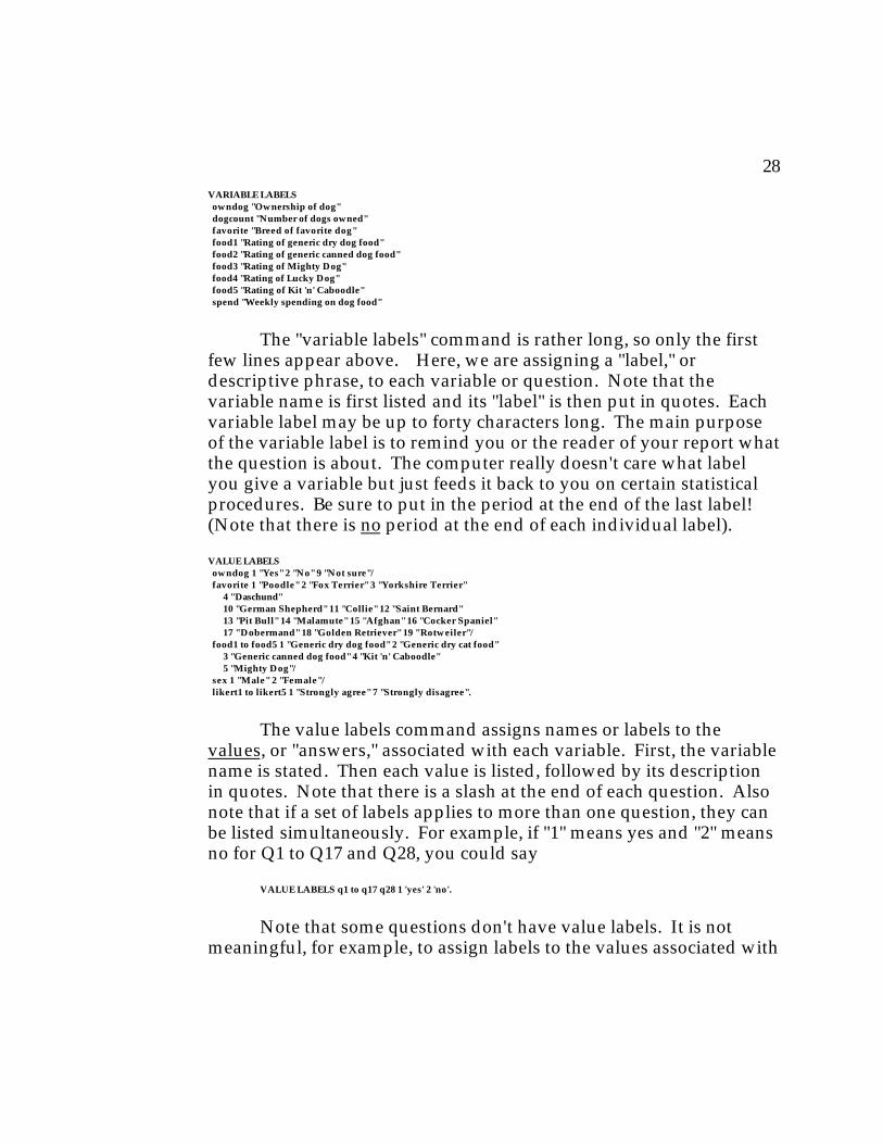
The "variable labels" command is rather long, so only the firstfew lines appear above. Here, we are assigning a "label," ordescriptive phrase, to each variable or question. Note that thevariable name is first listed and its "label" is then put in quotes. Eachvariable label may be up to forty characters long. The main purposeof the variable label is to remind you or the reader of your report whatthe question is about. The computer really doesn't care what labelyou give a variable but just feeds it back to you on certain statisticalprocedures. Be sure to put in the period at the end of the last label! (Note that there is no period at the end of each individual label).

VALUE LABELS owndog 1 "Yes" 2 "No" 9 "Not sure"/ favorite 1 "Poodle" 2 "Fox Terrier" 3 "Yorkshire Terrier" 4 "Daschund" 10 "German Shepherd" 11 "Collie" 12 "Saint Bernard" 13 "Pit Bull" 14 "Malamute" 15 "Afghan" 16 "Cocker Spaniel" 17 " Dobermand" 18 "Golden Retriever" 19 " Rotweiler"/ food1 to food5 1 "Generic dry dog food" 2 "Generic dry cat food" 3 "Generic canned dog food" 4 "Kit 'n' Caboodle" 5 "Mighty Dog"/ sex 1 "Male" 2 "Female"/ likert1 to likert5 1 "Strongly agree" 7 "Strongly disagree".

The value labels command assigns names or labels to thevalues, or "answers," associated with each variable. First, the variablename is stated. Then each value is listed, followed by its descriptionin quotes. Note that there is a slash at the end of each question. Alsonote that if a set of labels applies to more than one question, they canbe listed simultaneously. For example, if "1" means yes and "2" meansno for Q1 to Q17 and Q28, you could say

VALUE LABELS q1 to q17 q28 1 'yes' 2 'no'.

Note that some questions don't have value labels. It is notmeaningful, for example, to assign labels to the values associated with

29

AGE and INCOME since these are self-explanatory. This is the casefor most interval and ratio scaled variables; the quantity expressedusually carries its own meaning. (In some cases, you will probablywant to express the unit of measurement, such as pounds, inches,years, or dollars, in the variable label).

Both the "variable labels" and "value labels" commands areoptional and are available solely for your convenience. Putting themin will, however, tend to improve the readability of your output.

MISSING VALUE owndog likert1 to likert5 (9)/ dogcount favorite age (99)/spend (99.99)/income 999999.

We discussed the meaning of missing values in the chapter oncoding. Note that SPSS/PC+ will automatically interpret blanks asmissing values; thus you only put in those missing values you havedefined as referring to a non-legitimate missing answer. From theabove, you can see that the syntax is the variable name(s) followed bythe missing value in parentheses, separating each range by a slash.

BEGIN DATA.END DATA.

These two commands, both followed by a period, tell thecomputer that the data will now begin and stop, respectively. Inbetween, you can then type in the data as it is defined in the data list.

30

Sending OutputTo the Printer

By default, SPSS/PC+ displays the statistical output on thescreen. If, instead, you would like to send the output to the printer,simply put the following two lines in your program:

set more off.set printer on.

Whatever SPSS/PC+ produces after these commands areencountered in the program will be sent to the printer. Thus, if youdon't want to send your whole program to the printer, you can put thecommands immediately before the statistical procedures.

The "set more off" command frees you from having to press<RETURN> or <SPACE> at the end of each screenful of data. Thismeans that the output may "pass you by" before you have a chance toread it. If this happens, you may either want to leave out thiscommand or wait to read the output until you have it printed on paper.

Some printers, particularly laser printers and other printers thatuser single sheets instead of continuous "tractor" fed paper, causesometimes cause particular problems. See Appendix M for moredetails.

31

When typing in the data, be sure to check that you are "ontarget" with respect to the columns. Generally, all the lines should beequally long. Also, be sure to check that, when you have typed in acomplete entry, you are one column farther out than the last positionlisted in the data list.

FREQUENCIES VARIABLES=all/STATISTICS=all.

The "frequencies" command is an example of a statisticalprocedure or command--SPSS/PC+'s raison d'être. Once we havelooked through the data for errors, we will go over other statisticalcommands, which normally go here in the program, after anyrecoding and computations, which we will also discuss.

32

Step 3: Entering The Program And Data

There are several ways you can enter the program and datainto SPSS/PC+. Since SPSS/PC+ uses an ASCII, ("plain text") file tohandle the input data, you can either use REVIEW, the editor suppliedwith SPSS/PC+, or a word processor such as WordStar, WordPerfect,6or Microsoft Word. When using a word processor, be sure to set themargins so that the lines can be long enough. The default margins formost word processors will normally allow only about sixty-fivecharacters on a line.7 Be sure to save the file as an ASCII file, i.e. notin word processing format.

LOTUS 123 provides a nice way of entering data for smallquestionnaires. See Appendix E for details.

To use REVIEW, start SPSS/PC+. How you will do this maydepend on the setting of the computer you will be using. In somecases, there will be a "menu" on the computer, and all you have to dois to enter the number or letter that corresponds to SPSS/PC+. Onother computers, you may have to start from the DOS prompt. IfSPSS/PC+ is found on the "\SPSS" directory of the hard drive, youmight type in the underlined part of the following:

C:\>CD \SPSSC:\SPSS>SPSSPC

If neither of these approaches work, you will have to find"local" instructions for what do to. Fortunately, most of the rest of thismanual's approaches will be more universally applicable.

6

Use the text-in/text-out feature (<CONTROL> <F5>) to create anASCII file.

7Also notice that some word processors set margins in terms of lengthrather than characters. In the newer versions of WordPerfect or MicrosoftWord, margins are by default set in terms of inches. In such programs,you may wish to switch to a smaller font instead of adjusting the margins.

33

Once you are in SPSS/PC+, a logo will first flash and you willthen be presented with a menu. Press <ALT>-M, then <F3><RETURN>. Now specify the name you want to give the file8 thatwill contain your program and data and press <RETURN>. Forexample, if you were entering the questionnaire about dogs, youmight call it "A:POODLE.SPS." (It is traditional to use the file nameextension ".SPS," but if you like to be different, this convention is notrequired).

You are now in REVIEW, the editor associated with SPSS/PC+. To move around in the text you create, use the arrows to move upand down and in the right and left directions. When you are ready tosave, move to the top of the file (press <CONTROL>-<HOME>), press<F9>, and press <RETURN> twice.

If your file already exists, you will probably be brought into thedocument at the bottom. To go to the top, press <CONTROL>-<HOME>. (As you might expect, <CONTROL>-<END> will bring youto the bottom of the document). You can use the arrows on thekeyboard to move one space or line at a time. The <INS> key willtoggle between insert and write-over (that is, whether the computerwill type new text on top of existing text or move the old text over tomake room for the new). (The default is "on"; however, you may wantto turn it off if you are editing data and you want to overwrite someincorrect contents).

One tricky situation involves the insertion of a new line on thevery top of the file. (Suppose you want to insert "SET PRINTER ON"above the DATA LIST statement.) To do this, go to the top andinserting a blank space at the beginning of the line. You can nowpress <RETURN> and the blank line will be inserted at the top of thefile.

For some reason, REVIEW will occasionally save only what is

8If your floppy disk is in Drive A:, the filename should start with "A:,"e.g. "A:poodle.sps" in our case.

34

below the cursor. Therefore, you should always be sure to go to the top ofthe file before saving it. The complete sequence to save, including thisfirst step, is:

<CONTROL>-HOME><F9> <RETURN> filename <RETURN>

where "filename" represents a new filename and specification youmay optionally give the file. If you want to keep the "suggested"filename, just press <RETURN>.

Remember that SPSS/PC+ does not automatically save yourdata. Therefore, it is not a bad idea to save every fifteen to twentyminutes to guard yourself against a power surge or other interruptionwhich might destroy your data. Also, it is a good practice to have atleast two diskettes with the one being used as a backup.

You may not have time to type in all of your program and yourentire set of data in one sitting. You can leave REVIEW at any timeand resume at a later point.

35

Exercise

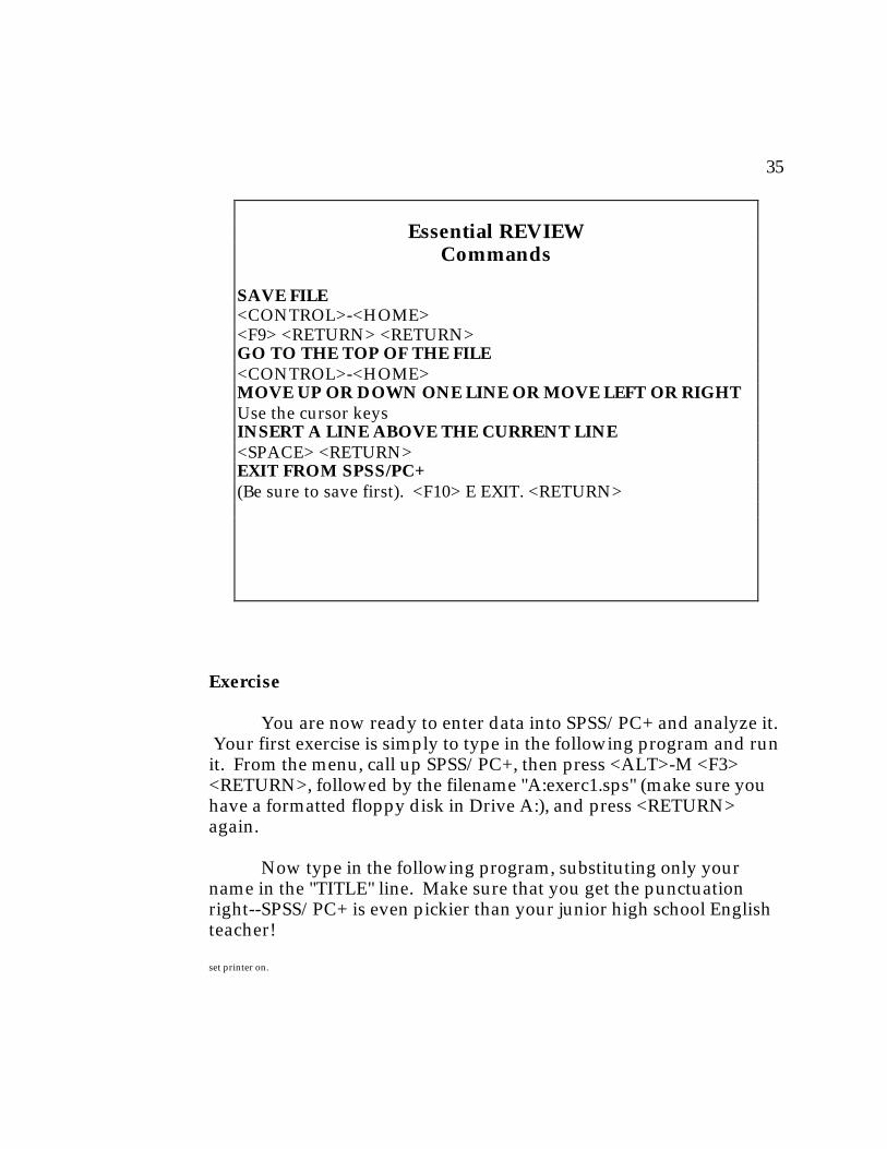
You are now ready to enter data into SPSS/PC+ and analyze it. Your first exercise is simply to type in the following program and runit. From the menu, call up SPSS/PC+, then press <ALT>-M <F3><RETURN>, followed by the filename "A:exerc1.sps" (make sure youhave a formatted floppy disk in Drive A:), and press <RETURN>again.

Now type in the following program, substituting only yourname in the "TITLE" line. Make sure that you get the punctuationright--SPSS/PC+ is even pickier than your junior high school Englishteacher!

set printer on.

Essential REVIEWCommands

SAVE FILE<CONTROL>-<HOME><F9> <RETURN> <RETURN>GO TO THE TOP OF THE FILE<CONTROL>-<HOME>MOVE UP OR DOWN ONE LINE OR MOVE LEFT OR RIGHTUse the cursor keysINSERT A LINE ABOVE THE CURRENT LINE<SPACE> <RETURN>EXIT FROM SPSS/PC+(Be sure to save first). <F10> E EXIT. <RETURN>

36

set screen off.title "YOUR NAME".data list /id 1 -3 age 5-6 educ 8-9 sex 11 income 13-15 vacation 17-20.variable labels age 'age of respondent' educ 'years of formal education completed' sex 'sex of respondent' income 'annual household income in hundreds of dollars' vacation 'amount spent by household on vacations last year'.value labels sex 1 'male' 2 'female'.missing value age,educ(99)/sex(9)/income(999)/vacation(9999).begin data.001 52 13 1 232 3270 2 50 13 1 235 4279 3 57 12 1 274 3643 4 30 10 1 217 3504 5 74 17 1 379 4247 6 63 15 1 353 3715 7 53 15 2 277 4059 8 57 16 1 294 4154 9 35 10 2 266 2908 10 38 11 2 234 3602 11 29 14 2 243 3492 12 24 11 1 185 3391 13 61 15 2 316 3637 14 47 12 2 225 3422 15 49 13 1 259 4289end data.frequencies variables=age to vacation/statistics=all.

You are now ready to run the program. Press <CONTROL>-<HOME> to go to the top, <F9> <RETURN> <RETURN> to save, and<F10> <RETURN> to run. If you have made a syntactic mistake,SPSS/PC+ may point it out to you and you will have to fix it andrerun.

Analysis

As is evident, this survey contains demographic informationabout surveyed individuals as well as information on how much theyspent on vacations.

1. Using the FREQUENCIES output you will receive, find themean, median, mode, and standard deviation for each variable. Dothose seem to be representative of the population at large?

37

Step 4: Checking Your DataAnd Program For Errors

So you thought that you were finally done with the programand data entry? Well, not quite yet! Your data is probably goodenough to be published in a tabloid magazine as it is, but there is oneadditional step that a conscientious researcher must take.

When you type in a large amount of data, there is a significantchance that you might make a typographical error. Not all errors canbe caught and some errors won't make that much difference, but someare relatively easy to catch and should be eliminated.

Now that you have all your data entered, make sure that thereis nothing below the "end data" line. (In our example, you woulddelete the "frequencies" line).

Now press <CONTROL>-<HOME> to go to the top of the file,press <F9> followed by <RETURN> <RETURN> to save, and <F10> torun. Unless you have turned the printer option on, you will get onescreen at a time. When a complete screen has been displayed, you willhear an obnoxious beep and you will be prompted with the message"MORE." Press <RETURN> to see the next screen.

The program may point out some errors in your program. Sucherrors are often caused by (1) omission of a period, quote, or slash, (2)the misspelling of a command or variable name, or (3) other"typographical" error. The computer will beep and stop after eachscreen of information has been displayed. Note down any errors andpress <RETURN> to continue.

Once the program has come to an end, press <F3> <RETURN>,followed by your filename and <RETURN>. You are now back inediting mode and you can now fix any problems you have been able toidentify. Continue running the program this way until all errors havebeen fixed.

Note that taking care of one error may fix several othercomplaints that SPSS/PC+ had in the previous run. If, for example,

38

you leave out a period or slash, SPSS/PC+ may encounter severalsubsequent "errors"--expressions that are not allowed in the givencontext. In other words, if you left out some punctuation, SPSS/PC+may expect something that is not forthcoming and will continue tocomplain.

Also note the way SPSS/PC+ chooses to describe your errormay not be very informative. The reference to "an unrecognizedexpression," for example, can mean almost anything. Instead, focuson where error occurs. Should there have been a period immediatelybefore? Did you misspell a command?

When you are satisfied that the errors have been removed fromthe program, add the line

frequencies variables=all.

to the bottom of the file, press <CONTROL>-<HOME> to go to thetop, <F9> <RETURN> <RETURN> to save, and then <F10><RETURN> to run the program. After going through the datadefinition part of the program, the computer will display thefrequency counts of each variable. You should now look for"illegitimate" values for each variable. Let's take a look at the belowexample:



Yes 1 82 46.9 49.1 49.1No 2 81 46.3 48.5 97.6Not sure 3 3 1.7 1.8 99.4

4 1 .6 .6 100.0Missing 9 8 4.6 MISSING

------- ------- ------- TOTAL 175 100.0 100.0

Valid Cases 167 Missing Cases 8

In this case, it is quite evident that an error has been made sincethere is no such legitimate value as "4" for this question. That is, youeither own a dog, don't own a dog, don't know if you own a dog, or

39

refuse to answer the question. Therefore, the code "4" cannotrepresent a acceptable answer. We now know that something wentwrong, and we will want to track down the error. Also note that wereally would have no way of detecting if the value of "3" had beenentered one time too many (at the expense of some other code) sincethat would not show up as an illegitimate value. Be sure to note downall unacceptable values. (In this case, there is only this one"objectionable" value). Note that the period indicates a "systemmissing value" (or a blank) and that "9" is our defined missing value tobe used when the given answer is not usable).

When you have found all the illegitimate values in theprogram, run the program again, this time putting in the followingtwo lines at the bottom:

PROCESS IF (dogown EQ 4).FREQUENCIES VARIABLES=id.

In the above example, you would modify the part inparentheses to meet the condition relevant to your case. On the leftside of the "EQ" put the name of the variable that gave you anoffending value and on the right side, put the value in question. Nowthe computer will select only the case that has given you the problem. The next line will give you the case number of the problem variable. When you run the program, you will identify the offending case andyou can make appropriate corrections.

Once you have weeded out the incorrect values, you may wantto run the frequencies check again to see if you got them all or if newones have come about as a result of editing.

40

Step 5: Using Statistical ProceduresAnd Computations

Statistical commands normally go at the bottom of the file,after any computation and recoding commands.

Frequencies

You have already been exposed to the Frequencies command,which provides a frequency count answers to each variable specified. The Frequencies command can give you more information, however. By saying

FREQUENCIES VARIABLES=all/STATISTICS=all.

you will get the mean, standard deviation, median, mode, and variousother statistics associated with the distribution.

DOGS Number of dogs owned or leased


.00 42 63.6 66.7 66.7 1.00 13 19.7 20.6 87.3 2.00 4 6.1 6.3 93.7 3.00 1 1.5 1.6 95.2 4.00 1 1.5 1.6 96.8 6.00 1 1.5 1.6 98.4 41.00 1 1.5 1.6 100.0 99.00 3 4.5 MISSING ------- ------- ------- TOTAL 66 100.0 100.0

Mean 1.190 Std Err .656 Median .000Mode .000 Std Dev 5.208 Variance 27.124Kurtosis 57.522 S E Kurt .595 Skewness 7.448S E Skew .302 Range 41.000 Minimum .000Maximum 41.000 Sum 75.000

Valid Cases 63 Missing Cases 3

For example, this table indicates that 42 of the people own orlease no dogs, 13 people have one, four people have two, and three,four, six, and forty-one dogs are possessed each by one person. Wehave missing data for three people, and the mean number of dogsowned is 1.19 (although the median is 0.00). It looks as though our

41

average has been brought up quite a bit by the person who ownsforty-one.

Creating New Variables: Compute

Computations can be very useful. Suppose you have collecteddata on how much people spend during Christmas for presents(GIFTS), comestibles (FOOD), travel (TRAVEL), and additionalChristmas related expenses (OTHER). If the variable names are theones given in the parentheses, you can calculate total Christmasexpenses (EXPENSES) by

COMPUTE expenses=gifts+food+travel+other.

If for some reason you wanted to find the average of thosefigures, you would say

COMPUTE avgexp=(gifts+food+travel+other)/4.

Recoding Variables

Recoding can sometimes be useful when doing crosstabs andother nominal statistics where you would like to "collapse" the data tomake it more interpretable. In our questionnaire, we might want tocollapse the AGE variable:

RECODE age (0 THRU 25=1) (26 THRU 40=2) (41 THRU 65=3) (66 THRU 98=4).

As is evident from the example above, you first state the nameof the variable. Each value range is then specified in parentheses,followed by an equal sign, and the desired recoded value.

Details on specific statistical procedures are found in theSPSS/PC+ manuals, however, the syntax for a few procedures iscontained below.

42

Reverse Scoring

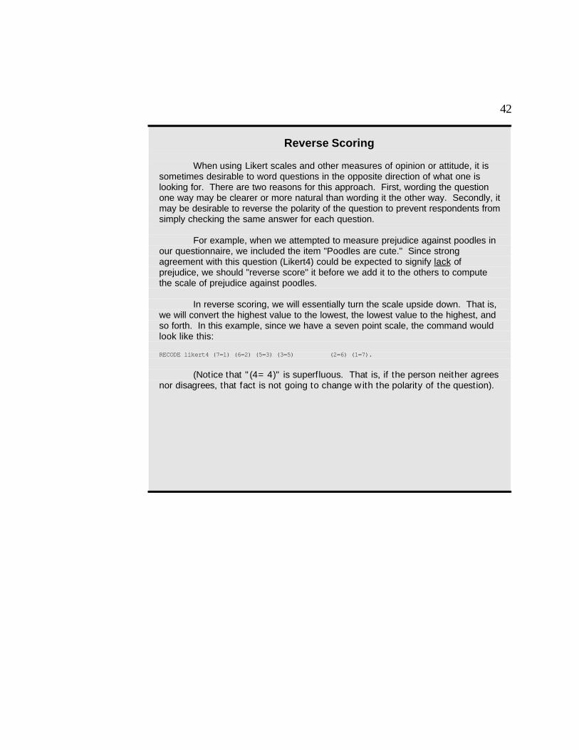
When using Likert scales and other measures of opinion or attitude, it issometimes desirable to word questions in the opposite direction of what one islooking for. There are two reasons for this approach. First, wording the questionone way may be clearer or more natural than wording it the other way. Secondly, itmay be desirable to reverse the polarity of the question to prevent respondents fromsimply checking the same answer for each question.

For example, when we attempted to measure prejudice against poodles inour questionnaire, we included the item "Poodles are cute." Since strongagreement with this question (Likert4) could be expected to signify lack ofprejudice, we should "reverse score" it before we add it to the others to computethe scale of prejudice against poodles.

In reverse scoring, we will essentially turn the scale upside down. That is,we will convert the highest value to the lowest, the lowest value to the highest, andso forth. In this example, since we have a seven point scale, the command wouldlook like this:

RECODE likert4 (7=1) (6=2) (5=3) (3=5) (2=6) (1=7).

(Notice that "(4=4)" is superfluous. That is, if the person neither agreesnor disagrees, that fact is not going to change with the polarity of the question).

43

Crosstabulation

A crosstabulation allows us to explore the relationship betweentwo variables by tabulating one against the other. Consider thisexample:

Crosstabulation: HEIGHT Height of customer By ANIMAL Species of preferred stuffed animal

Count �Giraffe �Elephant�Bear �Cow �Pig �Dog �

ANIMAL� > � � � � � � � Row

� 1 � 2 � 3 � 4 � 5 � 6 � Total

HEIGHT ��

1 � 6 � 10 � 14 � 5 � 21 � 4 � 60

Short � � � � � � � 33.3

��

2 � 4 � 10 � 16 � 5 � 19 � 6 � 60

Medium � � � � � � � 33.3

��

3 � 10 � 6 � 17 � 5 � 15 � 7 � 60

Tall � � � � � � � 33.3

��

Column 20 26 47 15 55 17 180 Total 11.1 14.4 26.1 8.3 30.6 9.4 100.0


6.17035 10 .8008 5.000 None With ANIMAL

As you will note, the values of one variable are listedhorizontally, and the values of the other are listed vertically. In thecells, you see the number of subjects falling into the "intersection" ofthe two. The table shows, for example, that fifteen people are bothtall and prefer pigs. You will notice that some statistics are alsoprovided. (We will soon get to why anyone would care about therelationship between these two variables).

The general syntax for crosstabs table is:

CROSSTABS TABLES=firstvar by secondv/STATISTICS=all.

where "firstvar" and "secondv" are the two variables you want totabulate against each other. Notice that the optional statistics take up

44

a lot of room. If you only want Chi square (χ2), you can reduce theoutput by substituting "STATISTICS=1" for "STATISTICS=all."

Or, you could select the statistics available from this list:

Ordinarily, you probably wouldn't want to look at anythingmore than statistics numbers one and two. However, calculating theothers won't take the computer very long at all, so there is littlepenalty in saying "STATISTICS=all."

If you want more detail, you can get row and columnpercentages, i.e. the percentage of the row and column that each cellcontributes, by putting in the "/OPTIONS=3,4" parameter. Thus, ifyou were tabulating "firstvar" with "secondv" and wanted thesefeatures as well as Chi square and Cramer's V, the command wouldbe:

CROSSTABS TABLES=firstvar BY secondvar /STATISTICS=1,2

/OPTIONS=3,4.

Statistics Available inCrosstabs

1 Chi square 2 Phi or Cramer's V, depending on the

number of variables 3 Contingency coefficient 4 Lambda 5 Uncertainty coefficient 6 Kendall's Tau-b 7 Kendall's Tau-c 9 Somers' d10 Eta11 Pearson's r

45

Note that the period goes at the very end of all thesubcommands. You would not place a period after "firstvar BYsecondvar" if you included additional subcommands as we did in thiscase.

If you want to create multiple tables with one command, youcan specify a variable list on each side of the "BY" part of thecommand. For example, you could say:

CROSSTABS TABLES=var1 to var5 by var6 to var10/ STATISTICS=1.

Notice, however, that this would create 5x5=25 tables! It iseasy to write a statement, without realizing it, that would createhundreds of tables. This would most likely provide you with severeinformation overload and would make any sort of meaningfulinterpretation impossible. For example, if you have thirty questionsand you want to see how "everything relates to everything," youmight think about saying "tables=var1 to var30 by var1 to var30." However, this would create 420 non-redundant tables! You would besitting by the printer for a long time and would probably not havetime to interpret all of them.

To find out in advance how many tables you would get bytrying a list of variables against the same list, use the formula

T = (n2-n)/2

where T is the resultant number of tables and n is the number of itemsin the list.

To find out how many tables would result from running twodifferent lists against each other, multiply the number of variables ineach list by each other. For example,

CROSSTABS TABLES=var1 to var10 by var15 to var20

would result in (10*6)=60 tables.

46

Let's suppose that you have been hired to do a marketing studyfor a manufacturer of stuffed animals. The manufacturer wants tostart a poster media campaign to promote his stuffed animals to thepublic. A media consultant (of questionable reputation) that he hashired believes that advertising will be most effective if it is placed ateye level. In order to enable the manufacturer to target customers ofdifferent height, the manufacturer has asked you to find out whetherthere is a relationship between a person's height and his or herpreferred stuffed animal species. You collect data and run thefollowing crosstabulation:



ANIMAL� > � � � � � � � Row

� 1 � 2 � 3 � 4 � 5 � 6 � Total

HEIGHT ��

1 � 6 � 10 � 14 � 5 � 21 � 4 � 60

Short � � � � � � � 33.3

��

2 � 4 � 10 � 16 � 5 � 19 � 6 � 60

Medium � � � � � � � 33.3

��

3 � 10 � 6 � 17 � 5 � 15 � 7 � 60

Tall � � � � � � � 33.3

��

Column 20 26 47 15 55 17 180 Total 11.1 14.4 26.1 8.3 30.6 9.4 100.0


6.17035 10 .8008 5.000 None With ANIMAL Statistic Symmetric Dependent Dependent --------- --------- ------------- -------------

Lambda .04898 .08333 .01600Uncertainty Coefficient .01260 .01585 .01045Somers' D -.02035 -.01877 -.02222Eta .15250 .05750


Cramer's V .13092Contingency Coefficient .18205Kendall's Tau B -.02042 .3730Kendall's Tau C -.02222 .3730Pearson's R -.03093 .3401Gamma -.02806

Number of Missing Observations = 0

47

Looking at the intersection of the two variables in the table, wecan see six people are both short and prefer giraffes, 16 medium sizedpeople prefer bears, etc. That is a large amount of information noteasily interpretable without any kind of statistical summary.

Is there a relationship between the two variables? It is difficultto say just from looking at the table. However, the Chi square (χ2)statistic will test the null hypothesis that the two variables are"independent," i.e. that knowing information about the one does nottell us anything about the likelihood of the other. Normally, werequire the significance level to be less than 0.05. Since we did notcome anywhere near that this time around, we conclude that there isnot enough evidence to support the height hypothesis, and werecommend to the manufacturer that he find another method ofsegmenting his advertising.

Product Moment (Pearson) Correlation

The general syntax for Pearson Correlation in SPSS/PC+ is:

CORRELATION varlist WITH varlist

/OPTIONS=options.

In practical terms, if we wanted to generate the below matrix ofthe (boring) variables X60 to X62 correlated against X63 to x65, wewould write:

CORRELATION x60 to x62 WITH x63 to x65/OPTIONS=5.

48

Correlations: X63 X64 X65

X60 .0267 -.0900 .0448 (<---coefficient)

( 72) ( 72) ( 72) (<---no. of cases)

P= .412 P= .226 P= .354 (<---significance)9

X61 .0350 .1456 -.0413 ( 72) ( 72) ( 72) P= .385 P= .111 P= .365

X62 .1223 -.2251 .1382 ( 72) ( 72) ( 72) P= .153 P= .029 P= .123

(Coefficient / (Cases) / 1-tailed Significance)

" . " is printed if a coefficient cannot be computed

The "/OPTIONS=5" statement provides for the printing of thenumber of cases and the one-tailed significance levels associated withthe respective correlation coefficient.

If you are not sure whether to expect a positive or negativerelationship between the two variables, you may want a two-tailedprobability associated with the correlation coefficient. You wouldthen add option 3, making the above statement:

CORRELATION x60 to x62 WITH x63 to x65/OPTIONS=3,5.

If you want to create a square matrix of variables correlatedagainst each other, you can simply say

CORRELATION varlist /OPTIONS=options.

Thus,

CORRELATION x60 to x65/OPTIONS=5.

would create a matrix of x60 to x65 against each other. Notice thatclose to half of the correlations would be redundant (i.e. X62 against

9

Note that, unless you change the options, this significance level isone-tailed.

49

X63 is the same as X63 against X62) and the coefficients of thecorrelations on the diagonal would be all ones since we are correlatingeach variable with itself. (That is, a variable perfectly "predicts"itself).

Multiple Linear Regression

There are three main methods of doing linear regressionanalysis within SPSS/PC+10: forward inclusion, backwardelimination, and stepwise. To run an analysis, you must make adecision as to which one to use. Theoretical and philosophicalconsiderations will enter your decision as to which method to select,but if you wanted to keep things simple, you would most likely useforward inclusion.

A regression analysis contains exactly one dependent variableand one or more independent variables. The syntax for thecommand is:

REGRESSION VARIABLES=varlist/DEPENDENT=depvar/METHOD=method.

Thus, to do a forward inclusion regression analysis trying to"predict" X38 from X3,X4,X5,X6, and X7, you would write:

REGRESSION VARIABLES=x38,x3 to x7/DEPENDENT=x38/METHOD=forward.

If you wanted to do a stepwise or backward eliminationprocedure, you would substitute the words "STEPWISE" and"BACKWARD," respectively, for the term "FORWARD."

Please note that, when doing a regression analysis, you are notguaranteed any result. If no predictor variables are significant at the

10

Some more esoteric varieties (such as hierchical regression) are alsoavailable but will not be discussed.

50

first step, the process will simply tell you that the "PIN limit" of .05 (orwhatever level you may have specified if you chose to override thedefault) has been reached and terminate. This is a frequent outcome,reflecting an empirical reality, and does not indicate that an error hasbeen made.

Also beware that the computer can calculate a meaninglessregression equation if the underlying assumptions of the model arenot met.

Discriminant Analysis

Discriminant analysis is a relatively complex topic. In order toperform this procedure appropriately, you will need a solidbackground in statistics. It is expected that you will have obtainedthis background from a statistical text or other appropriate sourceprior to reading this manual.

The procedure DSCRIMINANT (note the lack of "i" in thespelling) is found in the Advanced Module of SPSS/PC+. This meansthat you may not have access to this feature in industry even if yourcompany has the Base version of SPSS/PC+.

The syntax for the procedure is:

DSCRIMINANT GROUPS= vargroup(val1,val2)/ VARIABLES=predictor variables

/STATISTICS=statistics.

In the GROUPS specification, you indicate the values for eachof the two11 relevant groups within the appropriate groupingvariable. The variable specification parameter allows you to specify

11

Technically, it is possible to specify more than two groups. If, forexample, you were specified "GROUPS=CLEVEL(2,3,4)," you couldinvolve sophomores, juniors, and seniors in your analysis.

51

which variables you wish to attempt to use as predictors. Thus, if youwere trying to predict purchase of your product (purchase=1) vs. non-purchase of your product (i.e. no purchase or a purchase of yourcompetitor's product) (purchase=2), using income, sex, age,education, and various other demographic variables (DEMO1 toDEMO15), your procedure might look like this:

DSCRIMINANT GROUPS=purchase(1,2)/ VARIABLES=income,sex,age,educ,demo1 to

demo10/STATISTICS=1,2.

Since the specification of "STATISTICS=ALL" will normallyresult in a very voluminous output, it is recommended that youconfine yourself to "STATISTICS=1,2," which will give you the meanand standard deviations for each potential predictor variable brokendown by the two groups.

For more information, see the SPSS/PC+ Advanced StatisticsManual.

Count: "Counting" on how many variables a criterion is met

Sometimes, you may be interested in "counting" the number ofvariables on which subjects meet a certain criterion. In less abstractlanguage, you might be interested in knowing how many of a list ofproducts have been bought by a particular consumer. For example, ifwe wanted to know how many major brands of soft drinks a personhad bought and we had each of the major brands coded as anindicator variable (i.e. 1=purchase, 0=non-purchase), we might makea count as follows:

COUNT sdrink=drink1 TO drink10(1).

In the above example, we are interested in those variablesamong "drink1" to "drink10" to which people gave the answer 1(purchase).

52

Descriptives: A summarized version of Frequencies.

Descriptives (known as Condescriptive in the mainframe versionand in certain other packages) provides a summary of the statisticswhich appear in the frequencies table, such as the mean, median, andmode, without the explicit listing of the frequency of each response. This may be useful under certain circumstances, particularly whenyou are using interval data with many different values. For example,if you were to measure annual household income with a precision of$100, you might expect to get a large number of discrete answers iffrom a survey of several hundred people. Thus, you might be betteroff with a set of summary statistics including the mean, median,mode, and standard deviation, at least for inclusion in your report. (Note: You may still want to do a complete frequencies printout tolook for outliers).

Using the income example, the following command mightcreate the below table:

DESCRIPTIVES VARIABLES=income /STATISTICS=1,5,13,10,11.

Number of Valid Observations (Listwise) = 49.00

Variable Mean Std Dev Minimum Maximum N Label

INCOME 270.43 46.10 209 356 49 annual household inc

It goes without saying, but is worth reiterating, that"descriptives" would not generate a meaningful output for variablesin an nominal type scale.

For those technically interested, Descriptives can also be used tocreate z-scores, i.e. standardized scores measuring relative deviationfrom the mean rather than absolute magnitude. (This is useful whenyou want to run a regression analysis on data that has an odddistribution).

53

Npar tests: Non-parametric statistical tests.

SPSS/PC+ allows you to perform various non-parametric testssuch as Wilcoxon, Cochran, Friedman, Mann-Whitney, and variousothers. See the SPSS/PC+ Base Manual for details.

Means: Providing a breakdown of population means by subgroup.

Again, the title sounds a little esoteric, but the basic concept isquite simple. Sometimes, a single population mean may be deceptivebecause it is heavily influenced by some underlying variable. Suppose, for example, that we know that the average height of agroup is 69 inches (5'9"). We might find it useful to break down thisfigure by men and women, realizing that a lot of the variability is dueto between group (sex) differences:

Summaries of HEIGHT By levels of SEX



SEX 1 male 62.3200 3.5587 100SEX 2 female 55.5500 3.9603 100

Total Cases = 200

But we can do better than this. Suppose that we also know thathalf of the people are basketball players (bball=1) and half are not(bball=0). We can now do a breakdown at two levels. Notice that sexis still the outermost criterion for distinction since this is consideredthe stronger source of influence. (That is, we expect the average malenon-basketball player to be taller than the average female player).

54

Summaries of HEIGHT By levels of SEX

BBALL basketball player or not



SEX 1 male 62.3200 3.5587 100 BBALL 0 no 60.0800 2.6942 50 BBALL 1 yes 64.5600 2.8440 50

SEX 2 female 55.5500 3.9603 100 BBALL 0 no 53.1600 3.0463 50 BBALL 1 yes 57.9400 3.2789 50

Total Cases = 200

ONEWAY and ANOVA: Analysis of Variance

SPSS/PC+ allows for one way as well as more complexmethods of analysis of variance. For ONEWAY the syntax is:

ONEWAY VARIABLES=dependents BY independent(min,max).

where dependents refers to the list of dependent variables to be testedand independent refers to the criterion variable on which subjects areto be distinguished. "Min" and "max" refer to the minimum andmaximum values of the independent variable on which subjects are tobe distinguished. Thus, for example, if we have the followingoccupational groups:

1=construction2=other blue collar3=professional4=other white collar5=other

and were are interested in testing for income differences between thefirst four groups, our statement would look as follows:

ONEWAY VARIABLES=income BY occup(1,4).

55

The ANOVA program is somewhat more complex and shouldbe attempted only by individuals well versed in statistics. Details arein the SPSS/PC+ Base Manual.

Plot: Turning bivariate data into a scatterplot.

When you do a correlation analysis, you may come up with aresult like r=.33. From this, you may be able to deduce that the onevariable accounts for something like (.33)0.5=11.1% of the variabilityof the other. However, perhaps a plot of the two variables againsteach other might be more illustrative and help in your interpretation. To create a plot, use the PLOT command. The syntax for a plotsuitable for the above situation is:

PLOT FORMAT=REGRESSION/PLOT=var1 with var2.

where "var1" and "var2" are the names of the two variables you wantto plot.

For example, this plot displays the relationship betweenexpenditures on chocolate and spending at service stations among agroup of hypothetical consumers. The correlation is approximately.33.n

56

PLOT OF CHOCOL WITH AUTO ��

W 9� �

e � 1 �

e � �

k � 1 �

l � �

y 6� �

� �

c � R

h � 1 2 1 11 �

o � 1 1 2124 2123 12 �

c 3� 1 1 1 2313111 1 �

o � 1 23 211332 21 1 �

l R 1 112 22 1 1 �

a � 1 1 �

t � �

e 0� 1 1 �

��

30 50 70 90 20 40 60 80

Monthly spending at service stations

(The numbers indicate how many people fall approximately atthat point in the intersection of the two variables).

Plot allows a number of options which are described in themanual.

Reliability: Finding coefficient Alpha and other measures ofreliability in a scale

If you ask a question or about a concept in many severaldifferent ways or versions, you may be interested in attempting toinfer the reliability of the measure from the repeated measurements. Of particular interest may be coefficient alpha. Suppose you havecollected a survey containing a scale consisting of variablesPREJUD16 to PREJUD25, all measuring prejudice against poodles. Tofind coefficient alpha, the command would be:

RELIABILITY VARIABLES=prejud16 TO prejud25 /SCALE=prejud16 TO prejud25

/MODEL=ALPHA.

(It is not a mistake that the variable specification, "prejud16 TOprejud25," appears identically twice in the command).

57

Other models, such as split half and parallel forms, aredescribed in the Advanced Statistics manual.

t-test: Testing for differences in two population means.

There are two kinds of t-test commonly used. The one is used totest for differences between groups, as if we were going to test fordifferences in height between males (sex=1) and females (sex=2). Thesyntax for this kind of t-test is

T-TEST GROUPS=sex(1,2)/VARIABLES=height.

Another example: Is there a difference in the number of softdrinks consumed (sdrinks) by males and females?

T-TEST GROUPS=sex(1,2)/VARIABLES=sdrinks.

Independent samples of SEX

Group 1: SEX EQ 1 Group 2: SEX EQ 2

t-test for: SDRINKS beverages consumed prior to campaign

Number Standard Standard of Cases Mean Deviation Error

Group 1 100 28.2300 10.744 1.074 Group 2 100 30.4100 10.181 1.018

� Pooled Variance Estimate � Separate Variance Estimate

� �

F 2-Tail � t Degrees of 2-Tail � t Degrees of 2-Tail Value Prob. � Value Freedom Prob. � Value Freedom Prob.

� �

1.11 .594 � -1.47 198 .142 � -1.47 197.43 .142

The other kind is used to test for significant differences inrepeated measures or same-subject variables. Suppose we areinterested in finding out if people changed their consumptionpatterns of soft drinks after an advertising campaign. If we collecteddata on consumption both prior to (predrnk) and after (postdrnk) the

58

campaign, the syntax might look as follows:

t-test pairs=predrnk with postdrnk.

Paired samples t-test: PREDRNK beverages consumed prior to campaign POSTDRNK beverages consumed after campaign

Variable Number Standard Standard of Cases Mean Deviation Error

PREDRNK 200 29.3200 10.497 .742POSTDRNK 200 30.7800 9.887 .699

(Difference) Standard Standard � 2-Tail � t Degrees of 2-Tail Mean Deviation Error � Corr. Prob. � Value Freedom Prob.

� �

-1.4600 13.797 .976 � .085 .233 � -1.50 199 .136

Since the significance level associated with this test depends onwhether the test is one or two tailed, it is particularly critical that youmake hypotheses prior to running this test. For example, it might bereasonable to hypothesize that soft drink consumption would increaseafter the campaign, thus avoiding the need to allow for the left tail(that is, the probability that sales could also decline as a result of thecampaign). In any event, we must be careful to notice that even ifthere is a significant change, we cannot positively say that it wascaused by the advertising campaign. We hope, however, that this isthe best explanation available.

Advanced features: Factor, Cluster, Hiloglinear, and MANOVA.

The SPSS/PC+ Advanced Statistics Manual containsinformation about these more complex procedures. In general, theseshould be attempted only by individuals very knowledgeable aboutthe particular procedures since quite meaningless results can begenerated and misinterpreted by an inexperienced user.

59

Using Only Selected Cases

For some analyses, you may want to include only selectedsubjects in your calculations. For example, if you want to figure outthe average age of only those respondents to your survey who are dogowners, you might enter the following command:

PROCESS IF (dogown EQ 1).DESCRIPTIVES VARIABLES=age.

In the parentheses, we indicate a logical condition. In this case,the logical condition is that the value on the dog ownership variable is1.

Other logical "operators" are:

GT Greater thanGE Greater than or equalLT Less thanLE Less than or equalNE Not equal

Thus, if we wanted a Frequencies table of the number of dogsowned by people whose age is less than 35, we would say

PROCESS IF (age LT 35).FREQUENCIES VARIABLES=dogown.

60

Appendix ACommon Questions About

SPSS/PC+

Q.: I use SPSS/PC+ on a computer that is connected to a dot matrixprinter. Is there any way I can print the output from anothercomputer that has a better printer attached?

A.: Yes. SPSS/PC+ output is sent to the file C:\SPSS\SPSS.LIS. You can import this file into a word-processor and then movethe file over to the other computer (See Appendix I forinformation on how to import SPSS/PC+ output intoWordPerfect). Caution: Beware that SPSS/PC+ output is oftenvoluminous--printing all of it could be time consuming.

Q.: Sometimes, the arrow keys don't work while I am in SPSS/PC+. Did I do anything wrong?

A.: No. There is a bug that will often "invalidate" the arrow keysafter an SPSS/PC+ program has been run. The best way to getaround this problem is to save your data and reboot the system.

Q.: I have some LOTUS data I would like to analyze withSPSS/PC+. Do I have to retype it all?

A.: No. Either print it to an ASCII file (using PrintFile) or use theIMPORT command in SPSS/PC+.

Q.: Can I do nice graphics in SPSS/PC+?

A.: Although a graphics module is available, it has not beenpurchased by all institutions. Therefore, you are better off

61

creating graphs with a program such as LOTUS or HarvardGraphics. (For example, by typing in the information from afrequencies run, you could create a nice pie-chart).

Q.: I am really sold on SPSS/PC+ and I would love to have it athome. How do I go about getting it?

A.: Since SPSS/PC+ is a commercial product, it is copyrighted, andyou will have to buy your own copy. The Base version lists forabout $800 and contains the basic modules for such proceduresas frequencies, crosstabs, t-test, ANOVA, regression,descriptives, and means. The Advanced supplement costsabout the same and contains the modules for reliability, factoranalysis, and other advanced functions. You will need eight toten megabytes on your hard drive. You can, however, buy amore limited student version for about $40.

Q.: Sometimes when I press <ALT>-M <F3>, the computer beepsand says that the selection is not available in this mode. Whatwent wrong?

A.: The <ALT>-M is a so called "toggle" switch which changesbetween the menu and "type-in" modes. Apparently, you werealready in type-in mode before you started the command. Simply repeat the procedure (<ALT>-M <F3>), and you shouldbe able to continue.

Q.: I have noticed that some people use the menu system inSPSS/PC+ to write programs. Why isn't it covered in this text?

A.: It's true that the menus free you from typing in certaincommands in their entirety, but in the author's view, theycreate more problems than it solves.

62

Q.: What about the Data Entry module? Doesn't that save time?

A.: Some people find it easier to use this module, but since it has tobe purchased as a separate product, it may not be available toyou in industry, and it is therefore not a good idea to becomedependent on it. Also, if you are entering a long questionnaire,it is inefficient and frustrating to have to press <RETURN>after entering each variable.

Q.: I just have a short survey and all I want is some averages andperhaps some standard deviations. Do I really have to useSPSS/PC+ for this?

A.: No. Lotus 123 will allow you to compute the mean, standarddeviation, maximum, and minimum for a data range. Inaddition, you can do a regression analysis (DataRegression).

63

Appendix B

Working With SPSS/PC+Output

Everything should be made as simpleas possible, but no simpler than that.

--Albert Einstein

SPSS/PC+ allows you to do very complex analyses, includingsome whose interpretation would be challenging even for individualsholding advanced degrees in statistics and related fields. Therefore,we cannot cover the majority of analyses available, but in this section,we will attempt to look at the output from some of the procedurestypically used in a beginning research methods class. Specifically, wewill look at how to prepare output from the frequencies, crosstabs,and Pearson correlation procedures for analysis and interpretation.

Frequencies

Recall that the fundamental purpose of statistics is to makeinferences about some underlying population.12 Unless the samplesize employed is very large or unless the variability of the data is verylow, statistics based on a sample will rarely ever be exactly equal tothe population parameters. In some cases, however, statistics can begood estimates of the underlying population parameters, and we canuse statistical principles to evaluate the likely accuracy of ourestimate.

One approach to the assessment of the accuracy of a statisticalestimate is the use of a confidence interval. A confidence intervalrefers to the range within which a given proportion of statistics willoccur in repeated sampling of the same size from the respective

12

Figures based upon information about the entire population isknown as a parameter. By definition, there are no confidence intervalsassociated with parameters.

64

population. In less abstract terminology, if obtain, from sample data,a 95% confidence interval of $34,598 to $38,710 for the meanhousehold income in a neighborhood in which we are consideringopening a convenience store, we can be ninety-five percent certainthat the true population mean is within this range. There is, however,a 2.5% (5%/2) chance that the income is higher and a correspondingchance that they are lower.

65

Depending on the situation involved, you might be interested inone of two different kinds of confidence intervals, i.e. those for either

Warning!

Missing data can severely distort your statistics sinceSPSS/PC+ can only base its calculations on "valid" cases--that is,the cases that have a meaningful value for the variable in question. This is problem is particularly evident when we calculate the meanof a variable.

When you encounter a variable that has many cases missing,examine whether the missing cases may be systematically differentfrom the valid cases. For example, perhaps those people who didnot respond to a question of how many library books they checkedout last month don't care that much about libraries and checkedout fewer books than those who were conscientious enough toanswer the question.

Also, what is your population of interest? If you areinterested to find out how much the average person spends on dogfood, then those people who do not own dogs should not becounted as missing--instead, we would count those that appear tohave relatively normal eating habits as spending $0.00. If wecounted only those people who have dogs, we would greatlyoverestimate the market.

66

a mean or a proportion.

Confidence interval for a mean. We illustrated the idea that asample mean can be used to generate a confidence interval for apopulation mean above. Now, let's look at some SPSS/PC+ output13

to see how generate the data:

EDUC years of formal education completed


7 1 .4 .4 .4 8 1 .4 .4 .8 9 15 5.4 5.7 6.5 10 15 5.4 5.7 12.2 11 16 5.7 6.1 18.3 12 27 9.7 10.3 28.5 13 39 14.0 14.8 43.3 14 36 12.9 13.7 57.0 15 36 12.9 13.7 70.7 16 30 10.8 11.4 82.1 17 18 6.5 6.8 89.0 18 20 7.2 7.6 96.6 19 5 1.8 1.9 98.5 20 2 .7 .8 99.2 21 2 .7 .8 100.0 99 16 5.7 MISSING ------- ------- ------- TOTAL 279 100.0 100.0

Mean 13.970 Std Err .167 Median 14.000 Mode 13.000 Std Dev 2.710 Variance 7.343 Kurtosis -.408 S E Kurt .299 Skewness -.023 S E Skew .150 Range 14.000 Minimum 7.000 Maximum 21.000 Sum 3674.000

In the above survey, the respondents claimed to have a meanlevel of education of 13.97 years (i.e. being 0.03 years short ofcompleting two years of college). The sample standard deviation is2.71 years. Using the Lotus 123 spreadsheet MEANTINT.WK1 on thedistribution disk, get the result14

13

For this example, we will use information from a Frequencies printout,but you could also get the needed information from the procedure Means.

14For formulas, see an introductory statistics or research methods text.

67

Variable Sample Sample Sample Lower Upper Mean Std size (n) limit limit ---------------------------------------------------------------------- Education 13.97 2.71 263 13.64 14.30

From the above, we can conclude with 95% certainty that the"true" population mean is somewhere between 13.64 and 14.30 years. If we wanted to be more certain than that, the confidence intervalwould be wider.

Confidence intervals for a proportion. As you know, animportant step in business strategy formation is competitor analysis. Tallon Termite & Pest Control, a California company that uses liquidnitrogen to kill termites with "coldness instead of chemicals," isconcerned about aardvarks, the only other natural enemy thattermites have. The aardvark is commonly known as the ant-eater, butthat's a misnomer since, according to unverified companyintelligence, two out of three aardvarks prefer termites over ants. Although aardvarks reportedly chew with their mouths open, whichis not a pretty sight, they are could nevertheless represent a seriouscompetitive threat.

Let's suppose that you have been hired by Tallon Termite & PestControl, Inc., to assess the extent to which aardvarks constituteserious competition nitrogen program. You are directed to find outsnack preferences of the rivals by sampling one hundred aardvarksand asking if they prefer ants or termites. The results are as follow:

PREF Snack preference


Ants 1 26 26.0 26.0 26.0Termites 2 74 74.0 74.0 100.0 ------- ------- ------- TOTAL 100 100.0 100.0

68

Using the Lotus template PROPINT.WK1 on the distributiondisk, we get the following results, where p is the proportion ofaardvarks preferring termites and q is 1-p15, we obtain

Variable p q Sample Lower Upper size (n) limit limit ---------------------------------------------------------------------- Snack preference 0.74 0.26 100 0.65 0.83

Since we can conclude aardvarks are potentially a seriousthreat (we are 95% sure that between 65% and 83% of aardvarksprefer termites over ants), your next task is to find out whatpercentage of home owners in the company's trade area considersaardvarks' table manners offensive. Because the methodology is thesame, the task is left to you. (If funding is available, you mightexplore whether attitudes are influenced by whether a home ownerhas children of an age where they are particularly susceptible toinfluence).

Crosstabs

The crosstabulation feature is one of the more popularprograms in SPSS/PC+ since it allows the user to assess a relationshipbetween two variables when one or both of them are nominallyscaled. Note that in this example, the assignment of numbers tovarious categories of animals is nominal or arbitrary while thescaling for height is ordinal:

15

q is not always the equivalent of the proportion preferring ants. Insome cases, there may be several ways in which something can be "not p" without qualifying as q. For example, suppose that the aardvarks werealso given the choice "other." In that case, q would be equal to theproportion preferring ants plus the proportion preferring other snacks.

69



ANIMAL� > � � � � � � � Row

� 1 � 2 � 3 � 4 � 5 � 6 � Total

HEIGHT ��

1 � 6 � 10 � 14 � 5 � 21 � 4 � 60

Short � � � � � � � 33.3

��

2 � 4 � 10 � 16 � 5 � 19 � 6 � 60

Medium � � � � � � � 33.3

��

3 � 10 � 6 � 17 � 5 � 15 � 7 � 60

Tall � � � � � � � 33.3

��

Column 20 26 47 15 55 17 180 Total 11.1 14.4 26.1 8.3 30.6 9.4 100.0


6.17035 10 .8008 5.000 None With ANIMAL Statistic Symmetric Dependent Dependent --------- --------- ------------- -------------

Lambda .04898 .08333 .01600Uncertainty Coefficient .01260 .01585 .01045Somers' D -.02035 -.01877 -.02222Eta .15250 .05750


Cramer's V .13092Contingency Coefficient .18205Kendall's Tau B -.02042 .3730Kendall's Tau C -.02222 .3730Pearson's R -.03093 .3401Gamma -.02806

Number of Missing Observations = 0

Crosstabs provides a number of statistical tests. One of themore well known of these is the Chi square (χ2) test of independence,which assesses the probability that one could obtain a relationship inthe sample as strong as the one obtained if the sample were takenfrom a population in which no relationship actually existed. Theformula compares the ratio of the actual count in each cell to thatexpected under no relationship, given the distributions of eachvariable:

70

where k is the number of "cells" (i.e. different combinations of the twovariables), and Oi and Ei are the observed and "expected" number ofcases in the respective cell. SPSS/PC+ calculates the expectednumber of cases in each cell by multiplying the proportion of casesmeeting each condition and then multiplying by the total number ofcases. For example, if we have one hundred and eighty cases (n=180)and sixty people are tall (nT=60) and forty-seven people prefer bears(nB), then, if there is no relationship between the two variables, wewould expect a total of

(60/180) * (47/180) * 180 = 15.67

people to fall into the category of being both tall and preferring bears. This figure compares to the actual, or observed, count of seventeenpeople falling into that cell.

To each Chi square value corresponds a figure for degrees offreedom and a significance level. In our case, the significance level is0.8008, giving us insufficient evidence to reject the null hypothesisthat the two variables are independent. (Even if the Chi square valuehad been significant, we would not be able to conclude anything morethan that some kind of relationship probably exists between thevariables).

On the negative side, Chi square has some serious drawbacks:

1. It is not a powerful test, and we can only count on confirming a

71

relationship if it is strong. If you have interval data or betterfor both variables, you would be better off using correlation orsome other more powerful technique. Also, you are unlikely topick up a significant relationship with a small sample size.

2. It is not likely to yield significant results when there are many"levels," or possible values, associated with each variable. Variables having many levels should probably collapsed (e.g.on an age scale, you might collapse age 35-50 to one value).

3. When a large number of cells are empty, the test may not bevalid.

By specifying "/STATISTICS=ALL" when running Crosstabs,you get several other nominal level statistics. More details are in theSPSS/PC+ Base Manual.

Pearson Correlation

The Pearson correlation coefficient is used to assess the extentto which two variables can be used to "predict" each other. It istheoretically assumed that the two variables are both at least at theinterval level; however, in practice, the Pearson correlation coefficientis often used when one or both of the variables in question are onlyordinal. When assumptions are violated in this manner, any truerelationship between the two variables may be underestimated orentirely overlooked. Using a variable that does not achieve intervalor ratio scaling could also lead to an overestimate of the truerelationship, but that is less likely.

In practice, many researchers include Likert scale items, whichare ordinally scaled variables, in correlation analysis.

72

Also note that correlation is intended to explore any linearrelationship between two variables. That is, it is assumed that thechange in one variable as a result of the change in the other will beconstant regardless of the magnitude of either variables. For example,if we correlated grocery spending against income, it would beassumed that a $1,000 increase in come would result in the sameincrease in grocery spending whether the original income were$18,000 or $249,500. If this assumption is not viable, you may want totransform one or both of the variables. This topic is beyond the scopeof this book, but is generally covered in methodology texts.

Assuming you specified "Options=5" when you ran the analysis,your output will consist of three parts. Let's take a look at a fictitiousexample between income and vacation spending:

Correlations: VACATION

INCOME .5636 ( 263) P= .000

WARNING!

Pearson correlation coefficients are completelymeaningless when one or more of the variables isnominal (categorical). If we survey people for theirpreferences for soft-drinks and "1" corresponds toCoke, "2" corresponds to Pepsi, and "3" corresponds to"Sprite," the fact that Sprite drinkers may be specialand "reaching for more" doesn't make them exactlythree times as much of anything as Coke drinkers. (Touse categorical data in correlation or regressionanalysis, you can compute indicator variables, whichhave metric properties, and use those instead).

73

The first figure is the sample correlation coefficient. Thisranges between -1.0, when there is a perfect negative correlationbetween the two variables, and 1.0, when there is a perfect positivecorrelation between the variables.

On the second line, the number of cases on which thecorrelation is based appears in parentheses. Sometimes, this may be alower figure than your total number of subjects because there may bemissing data among some of your subjects16. Some people, forexample, might have felt that one or more of these questions was toopersonal to answer.

Finally, on the last line is the significance level associated withthe correlation coefficient. As we noted above, the figure of .5636 isthe sample correlation coefficient and may not be the actualpopulation coefficient.17 The significance level is the probability that thecorrelation coefficient is zero, not the probability that it differs from thefigure shown (which it probably will). It cannot be concluded fromthe above information (without making further calculations) that thepopulation correlation coefficient is greater than, say, 0.35. However,the sample coefficient is our best available estimate.

Now, what is the meaning of a correlation coefficient? Ingeneral, the rule says that the square of the value of the coefficientrepresents the proportion of the variability of the one variable"explained" by the other. For example, in the above example,

.56362= .3176,

suggesting that income "explains" about 31.76% of the variation invacation spending between people.

16

Note that a case will be missing in correlation if the only one of thetwo variables is missing.

17Because we are taking a finite sample from a population, we expect

our sample results differ somewhat from those of the actual population.

74

Correlation coefficients are not very intuitive. Sometimes, avisual representation is more informative. Using the Plot command,we get the following illustration: PLOT OF INCOME WITH VACATION ��

a 400� 1 �

n � 1 1 �

n � 1 1 1 1 1 2 1 �

u � 11 3211 1 31 1 1 R a � 1 3515221412 1 1 �

l 300� 2131115341221213 11 �

� 2 22 23422 5434111 �

h � 2 1 1 2 15216352 36 42 1 �

o � 1 2112521314132 1 1 �

u � 1 1 1 121 13 22 1 11 �

s 200� 1 111 121 1 1 �

e R 1 11 12 1 2 522 2 1 �

h � 21 1 1 1 �

o � �

l � �

d 100� 1 �

��

2000 2800 3600 4400 2400 3200 4000 4800

amount spent by household on vacations l

(The numbers in the box represent the count of cases falling atthat coordinate. In a perfect correlation, all the numbers would havebeen on a diagonal; with a complete lack of correlation, the numberswould have been scattered around the box without pattern).

75

Appendix C

Working WithLarge Data Sets

In Chapter 2, we discussed how a case can take up more thanone line. We noted that in the "data list" command, we mark thebeginning of a new line by a slash. Thus, if we have ID1 and questions1 through 50 on line 1 and ID2 and questions 51 through 100 on line 2,our data list might look like this:

data list /id1 1-3 q1 to q50 5-54 /id2 1-3 q51 to q100 5-54.

Two cases might look like this:001 80053594603668932848906761501037537601345684443947962001 23073741805274028467403200920734931437934283227406462002 37523313809651941755581798497615730965614784546728377002 19023558532353565640285040717661639182211365682678986

Now suppose that instead of just two lines per case, we have adata set that requires five lines per subject. Two cases, using thatsystem, might look like this:

001 51881042413879258528815244790246113226620946180660912001 17360960447695181568034889642259507514245342577273341001 90272540808655925656834500842489437576499768779375834001 85877256735693738165767968166614884079224430157401661001 93770572368521277158218564000020348310063127470916776002 28192629327531949569666071329351801708701532387853052002 46719233470503286424781463574656343764730263589509917002 56568263273220578001682471949627692765870597258624634002 92326111451257030599355546291915734015614726564885112002 85184875444974819662113452795996745459258090787424135

That format is not very readable. If you accidentally leave outone line from a case or put it in twice, the computer would warn youthat you that the number of lines is not evenly divisible by the numberof lines per case, but it might be difficult, or at least laborious, to trackdown where the problem occurred. Therefore, we might want to taketwo preventive steps:

1. First, assign a variable to each line to identify its number. Thus,

76

you might have a data list beginning like this:

data list /id1 1-3 line1 4 q1 to q50 6-55 id2 1-3 line2 4 q51 to q100 6-55

and going on like that until five lines have been created. For every case, then "LINE1" would be equal to "1,""LINE2," to 2, etc.

2. At the end of the five lines, create a data line that only containsthe one "variable" called "BOGUS." This will create a blank linethat makes it more obvious where each case ends. Note thatyou must assign the columns that "BOGUS" could take up eventhough the variable will be "system missing" for all cases. Wewill just say that it occupies column 1 of line 6. The completedata list from the above might look like this:

data list /id1 1-3 line1 4 q1 to q50 6-55/id2 1-3 line2 4 q51 to q100 6-55/id3 1-3 line3 4 q101 to q150 6-55/id4 1-3 line4 4 q151 to q200 6-55/id5 1-3 line5 4 q201 to q250 6-55/bogus 1.

Two cases from this data set might look like this:

0011 518810424138792585288152447902461132266209461806609120012 173609604476951815680348896422595075142453425772733410013 902725408086559256568345008424894375764997687793758340014 858772567356937381657679681666148840792244301574016610015 93770572368521277158218564000020348310063127470916776

0021 281926293275319495696660713293518017087015323878530520022 467192334705032864247814635746563437647302635895099170023 565682632732205780016824719496276927658705972586246340024 923261114512570305993555462919157340156147265648851120025 85184875444974819662113452795996745459258090787424135

If your data set becomes so big that it takes a long time to run,you might consider making a "system file," which will increase theexecution speed considerably. See Appendix D for more information.

77

Appendix D

Using System Files

So far, we have had to run our program each time we wantedto execute a series of one or more statistical procedures. This isgenerally the easiest way to work when your data set is small. However, as you noticed, running the program and having thecomputer "read" the data each time takes a great deal of time. Thebigger the data set, the more time it takes to run the program.

Creating a "system file," which stores the data in a way thatenables the computer to access it more quickly, may help you makethe reading of the data go faster. There are a few costs associatedwith this, however:

• It takes time to create the system file • The system file takes up a great deal of space on the hard disk.

If the computer is found in a college computer lab, there maynot be space enough on the hard disk for everyone to store hisor her data as a system file, and you may not be able to fit allyour data on a floppy disk.

• Although variable and value labels will show up in your outputas usual, you no longer have much of the information you usedto create your program in your file. If you forget a variablename, you may either have to refer to a printout or "get" the fileto find this information.

To create a system file, first type in the SPSS/PC+ program andthe data as you normally would. When finished, you may want to runa Frequencies procedure to find out if there are any errors in the data. You can also do any data modifications (such as Recode and Computestatements) now. When you are satisfied with the shape of your data,add a "save" statement to the very end of your program:

SAVE /OUTFILE="filename.SYS".

78

where "filename" refers to the name you want to give the system fileyou are creating. If your data file is named "SURVEY.SPS," forexample, you might want to name the system file "SURVEY.SYS." (Ona floppy disk in Drive A:, this would be "A:SURVEY.SYS." Note,however, that there might not be enough space on a floppy disk toaccommodate a system file containing a large data set.)

Now you are ready to access the system file for further analysis. To do that, create a new file (say, "FASTSURV.SPS"). Put in a "get"statement as the very first line in this file:

GET /FILE="filename.SYS".

where "filename" refers to the name of your system file.

After the "get" statement, you can add any statisticalprocedures and run the program as normal. Thus, in our example, arun involving a system file might involve the following:

GET /FILE="fastsurv.sps".CORRELATION age WITH income.CROSSTABS TABLES=dogpref BY sex.

79

Advanced Tip

Your data file might contain some redundant andunnecessary information that you don't want to includein your system file. For example, if you have five linesof data, you might have five lines of data (e.g. ID1, ID2,ID3, ID4, and ID5) and five line identification numbers(e.g. LINE1, LINE2, LINE3, LINE4, and LINE5). Toexclude these variables from your system file, use the"drop" subcommand of the Save command. If we wantto get rid of the above variables and our file and wewant to name our system file "SURVEY.SYS," thecommand would look like this:

SAVE /OUTFILE="survey.SYS"/DROP=id1,id2,id3,id4,id5,line1,line2,line3,line4,line5.

WARNING: In this case, "ID1 to ID5" would notbe equivalent to "ID1,ID2,ID3,ID4,ID5" since there area lot of variables that come in between theidentification numbers. Thus, if you said "/DROP=ID1to ID5," you would be excluding all but the last line oftext!

80

Appendix E

Importing Data FromLotus 123

Sometimes, you may want to analyze some data you alreadyhave typed into LOTUS 123 in SPSS/PC+. There are at least twosituations in which this could happen. First, suppose started anassignment in LOTUS 123. Later, you realize that you wish to dosome statistical analyses not available in LOTUS. The secondpossibility is that you may want to do some of your data input on acomputer that has LOUTS, but not SPSS/PC+, installed.

The following will illustrate how you can import sets of datathat consist of at most one line per case into SPSS/PC+. (If you havemore than one line of data, you will most likely have to use anSPSS/PC+ system file. See Appendix D and the section on Import inthe SPSS/PC+ Base Manual.) Since you already have the dataentered into LOTUS, it is assumed that you are reasonably familiarwith the program.

81

First, get into LOTUS 123 and bring up the file that contains thedata you wish to use in SPSS/PC+. Make sure that your data isaligned properly in the columns by issuing the "/Range Format Fixed"sequence of commands.

Now make sure that the data does not take up more than eightycolumns or spaces. If it does, you might try to reduce the length byfirst reducing excess columns assigned to any one variable. Forexample, while LOTUS assigns nine digits to each column by default,you don't need that many for a variable like age. (For reasons beyondthe scope of this book, you need one more column than the number ofdigits of the greatest number.) To reduce the number of columnsreserved for age to three, get into the column containing the age andissue the directive "/Worksheet Column Set width" and then specify3. If your data still does not fit, you might think about only takingsome of the variables into SPSS/PC+. You can do that by moving onlythose variables you want into another area of the spreadsheet.

Warning!

Lotus is not very strict about whether you put your casesacross rows or columns. That is, when you put the first variablefrom a case in a cell, you have a choice between putting the nextvariables to the right of this variable or below. For example, if youput VAR1 in A1, you can either put variables 2 through 5 in A2..A5or B1..E1.

SPSS/PC+ is a little more choosy. In SPSS/PC+, variablesassociated with the same case must occur in rows. This means thatif you put the first variable in A1, the next one should go in A2. Then variable 1 of the next case might then go in B1.

82

To take the data to SPSS/PC+, we will now "print" the variablesto an ASCII (i.e. plain text) file. You may be familiar with the "/PrintPrinter" command. Now instead say "/Print File." The computer willprompt you for the name of the output file. Let's call it "A:LOTUSDAT.SPS." (Make sure you have a formatted disk in driveA:.) Press "Range" and specify the range you want to take intoSPSS/PC+. Now specify "Options" in the print menu and choose"Margins Left" and specify "0." Finally, press "Align Go." When thecomputer has finished "printing" to the disk, that is, when the menucomes back, choose "Quit," then "/Quit" to exit LOTUS 123.

Now get into SPSS/PC+ and get into the file"A:LOTUSDAT.SPS" (i.e. by <ALT>-M <F3>).

83

Warning!

Even when you "print" to a file, LOTUS stillthinks in terms of a "sheet" of paper. Since a "sheet" inLOTUS cannot be set to be longer than 100 lines (withthe default being 66 lines), you will have some emptylines when each "page" ends in the file. Once you getinto SPSS/PC+, be sure to delete these empty lines.

Once you are in SPSS/PC+, it is time to put in the SPSS/PC+commands. You can get the information for the data list command bycursoring over the beginning and end of each variable and looking atthe position indicator in the bottom right part of the screen. Theninsert the needed statements such as Data list, Begin data, End data,and any Variable labels, Value labels, and Missing value definitions thatyou would like.

The program will now run just like any other program.

84

Appendix F

Similarities Between SPSS/PC+and Lotus 123

There are some similarities between some SPSS/PC+ functionsand those in Lotus 123 that you may already know. Let's suppose youwant to add up a person's total utility expenditures from his or herphone, water, natural gas, and power bills. In Lotus we might havethe data entered as follows:

A B C D E F

1 Phone Water Gas Power2 ---------------------------------------------------------------3 33.99 11.44 23.44 29.954 144.54 12.34 53.60 44.455 67.41 9.50 22.34 34.356 34.45 10.51 34.45 29.45

To add up the first person's total utility expenditures, youmight type in the formula

@SUM(A3..D3)

in cell E3. Alternatively, you could use the expression

+a3+b3+c3+d3 .

After you completed the calculation for the first case, youwould have to copy the formula from E3 to E4 through E6:

/cE3 <CR> E4..E6 <CR>.

Now look at how similar the procedure is in SPSS/PC+! Assuming that we already have created the variables PHONE,WATER, GAS, and POWER, we can use the latter approach from lotus

85

and say:

COMPUTE total=phone+water+gas+power.

(Unfortunately, there is no function comparable to @SUM inSPSS/PC+). For practical purposes, SPSS/PC+ will automatically dothe "cell copying" for us! (Remember, for statistical purposes wegenerally work with the entire data set without specific interest inindividual cases).

SPSS/PC+ provides other functions as well. These include boththe traditional ones such as the absolute value, e.g.

COMPUTE differnc=abs(score1-score2).

and more esoteric ones such as logarithmic and trigonometricfunctions18, which are also available in Lotus (See p. C-24 of theSPSS/PC+ v. 2.0 Base Manual for more information).

You can also use arithmetic expressions in calculations. Whilein Lotus you might multiply by putting the expression

+A12*A13

in cell A14, you might say

COMPUTE interest=prncpal*rate.

in SPSS/PC+.

18

For those interested in econometric and forecasting methodology, itis also possible to use lagged data. Details are found in the manual.

86

Important Note!

In Lotus, you are used to the automaticupdating which takes place when you change thevalues in a cell on which a formula is based. InSPSS/PC+, such updating will generally not takeplace. Consider this example of a commandsequence in SPSS/PC+:

COMPUTE discret=income-expenses. COMPUTE income=income*(1-taxrate).

SPSS/PC+ will not adjust discretionaryincome for the effect of taxes in this example! Toaccomplish this task, the second COMPUTEstatement would have to precede the first. In otherwords, the effect of the change in the incomecalculation is not "retroactive" as it would have beenin Lotus if you had gone back to change the formulain the cell in which (pre-tax) income was computed. It will, however, be in effect any time after the changehas been performed.

87

5551515555 084095098

Appendix G

Similarities Between SPSS/PC+and dBase III+

Readers familiar with dBase III and similar database programsmay notice certain conceptual similarities in SPSS/PC+. Althoughunderstanding how database software functions is not necessary tounderstanding how SPSS/PC+ works, it may help you understandsome concepts more easily.

First of all, both SPSS/PC+ and dBase clearly divide the datainto individual cases or "records." In dBase, the data associated witheach entity is kept within a single record. Thus, if we have a databaseof student grades, a dBase record might look like this:

In SPSS/PC+, each case is assigned a specific number of lines. Thus, our SPSS/PC+ case might look like this:

Each record or case is further subdivided. In dBase, we calleach variable a "field." For example, the field "MIDTERM" containsthe student's midterm score of 84. In SPSS/PC+, the variables are

Record 1

ID 5551515555MIDTERM 84PAPER 95FINAL 88

88

assigned specific column positions. If we look immediately after theblank space following the ID number (probably the student's socialsecurity number), we can see the entry of "084," signifying the score of84. Notice that the separation of the variables is completely up to us;we defined a blank space between the ID number and the scores, butnone between the scores themselves.

dBase allows us to compute several statistical functions. Thus,we could use the "average()" and "std()" functions to get much thesame information we could get with "descriptives" command inSPSS/PC+. However, dBase does not give us a direct way to doanything as complicated as crosstabs, correlation, regression, or evenfrequencies.

Sometimes, we are only concerned with part of our sample. Thus, in dBase, if we wanted to find the average on the final for thosepeople who scored below 70 on the midterm, we could say

AVERAGE(final) FOR midterm<70

while in SPSS/PC+, we might issue the commands

PROCESS IF (midterm LT 70).DESCRIPTIVES VARIABLES=final.

89

Appendix H

SPSS-X: The Mainframe Version

As mentioned in the introduction, a mainframe version, knownas SPSS-X, is also available on many university campuses. There are certain circumstances under which it may be desirable to use themainframe. Some features are not readily available on the PC or maytake too long to execute. This will normally not be a problem exceptyou wish to undertake very advanced analyses.

Another advantage of using a mainframe computer is thatmany university computer centers have a "high speed" printerconnected to their mainframes. These printers can often print out ahundred pages in less than one minute. Although you normally haveto wait for the printouts to be distributed to an "out" box at somecentral location, you at least save the time you would have to sit infront of a slower "ordinary" printer.

SPSS-X commands are very similar the SPSS/PC+ commands,the main exception being that there are normally no periods after theend of each command. You may also have to include some "filehandle" commands under certain circumstances and, of course, youwill have to deal with some computer commands very different fromthose of the IBM PC.

Extensive documentation on the use of SPSS-X is available fromSPSS, Inc. You may also have to get some handouts on yourmainframe's implementation of SPSS-X.

90

Appendix I

Incorporating SPSS/PC+ Output IntoWordPerfect Reports

Sometimes, you might like to include the results of a statisticalanalysis in a report. While it is possible to manually type the resultsfrom your computerized analysis into a word processing document, itcan be cumbersome and the complexity involved can lead to anumber of mistakes. Fortunately, there is an easier way.

SPSS/PC+ creates an output file to which everything you see onthe screen or on printer output is sent. This file, called"\SPSS\SPSS.LIS," is overwritten every time you restart SPSS/PC+, soyou will have to "rescue" the material immediately if you need it.19

Although this manual will illustrate the use of WordPerfect 5.0or 5.1 to "grab" important output, most word processors will providethe same capability.20

Immediately after you exit SPSS/PC+, select WordPerfect fromthe menu. If you have already created the document in which youwould like to include SPSS/PC+ output, call it up now. Regardless ofwhether you take that step or not, now switch to document #2(<SHIFT>-<F3>). Use the "text-in" function to retrieve the file"\SPSS\SPSS.LIS":

<CONTROL>-<F5> 1 2 C:\SPSS\SPSS.LIS <RETURN>

Find the part of the output you would like to include in your

19

Alternatively, can use the "SET RESULTS" command to direct youroutput to a permanent file (see manual).

20SPSS.LIS is an ASCII file and should be edited and read in

accordingly.

91

document and use the block function (<ALT>-<F4>) to mark theappropriate text. To copy the text, use <CONTROL>-<F4> to copyand press <SHIFT>-<F3> to move back to document #1. Use thecursors to move where you want the text inserted, then press<RETURN>.

If you want more text from the output, you can repeat theprocess.

NOTE: In some cases, the lines of SPSS/PC+ tables are morethan 65 columns long. If you encounter such a table, you will want tobe sure to use a font smaller than the default Courier, 10 pitch. Usethe base font option (<CONTROL> <F8> 4) to select. (The SPSS/PC+output included in this text was printed in Letter Gothic, 16.67 pitch).

Also, beware that you should never use a proportionally spacedfont for tables. (Helvetica and Times Roman are two of the mostcommon proportionally spaced fonts). While text printed in aproportionally spaced font looks very beautiful, this scheme tends todistort tables that depend on proper alignment of variables.

92

Appendix JDealing With Printer Problems

Unless you specify otherwise, SPSS/PC+ assumes that you areprinting to printer that uses continuous sheets of paper, each of whichis sixty-six lines long. This is fine when you print to dot matrixprinters whose paper is "tractor fed."

However, you may run into some problems when you try toprint to a laser printer or other kind printer that prints on stacks ofsingle sheets of paper. This happens because, although there is roomfor sixty-six lines of text on a laser printer, not all of the space on thepaper is available for the printer's use. Thus, the pages may becomedisalligned; that is, the page breaks may not occur at the right places.

To deal with this problem, enter the following series ofcommands where you would otherwise place the "set printer on"command:

SET SCREEN ON.SET MORE OFF.SET LENGTH=59.SET PRINTER ON.SET EJECT ON.

Be sure to enter the commands in the suggested order.

NOTE: When SPSS/PC+ is done printing, you may need topress the <FORM FEED> key on the printer to get the last page out.

93

Appendix K

Statistical Significance

When studying a subject such as statistics, it is easy to lose sightof the forrest for the trees (or, in more contemporary terms, to losesight of the computer for the chips). In order to get the "big picture" instatistics, it is important that you remember the fact that statistics isall about making inferences about an underlying population from alimited sample. If you do a study of grocery shoppers, you really don'tcare in particular about the people you are interviewing. A samplemade up of 100 people is in and of itself irrelevant (it is a very smallpart of the total market). You are really interested in generalizing theresponses of the sample to the population as a whole. This is not tosay that the selection of your sample is not important. In order tomake sure that the sample is representative of the population, theresearcher should use a sampling scheme that ensures properselection. Depending on the circumstances, one may want to useeither a random or systemematic sample or some variation of these.

As you know from introductory statistics, a sample mean willrarely ever equal the "true" population mean. You may recall theCentral Limit Theorem, which suggests that the larger the samplesize, the closer its mean will be to the actual population mean. Ingeneral, the principle that a larger sample size will allow you to makemore precise statistical inferences applies to other statisticalprocedures, too.

Every profession has its peculiar jargon, and statistics is noexception. One of the common terms in this field is that of statistical"significance." Despite what the word suggests, statistical significancehas nothing to do with importance. As ironic as it sounds, somethingcan be very significant but not at all important. Consider this fact: There is a statistically "significant" relationship between the numberof people at a Southern California beach and the number of leaves onthe surrounding eucalyptus trees. (This is, in terms of another piece of

94

statistical jargon, a spurious correlation in the sense that both of thesephenomena are "caused" by a common factor [the season of the year]although there is no intercausal relationship between the two).

In the broadest possible terms, statistical significance refers tothe probability that one would observe a sample statistic as extremeas the one obtained if, in fact, there were no such relationship in thepopulation.

You will recall from your statistics classes the use of the nulland alternative (or "research") hypotheses (Ho and Ha). You assumethe null hypothesis, which states that there is no relationship, to betrue until you find overwhelming evidence that it is not--in that case,you "accept" the alternative hypothesis, knowing that there is acertain chance (e.g. 5%) that the relationship does not exist.

Consider this fictitious example: A researcher samples fiveathletes and five non-athletes to see how many soft drinks they eachconsumed last week. The results are as follows:

Soft drinks Standardconsumed deviation n

_______________________________________________Athletes 19.1 7.7 5Non-athletes 14.9 6.5 5

Intuitively, would you be confident in concluding that athletesdrink more soft drinks than non-athletes? Although you could do a t-test to be sure, you would probably conclude without doing so thatyou don't have enough evidence to conclude that there is a difference. (This would particularly be the case if you had you had not made ahypothesis in advance that athletes drink more soft drinks than non-athletes). The fact is that the variance within each group is so highcompared to the difference in the two sample means suggests that noconfident conclusion is possible. Now let's suppose, however, that wesampled ten thousand athletes and ten thousand non-athletes and gotthe following results:

95

Soft drinks Standardconsumed deviation n

_______________________________________________Athletes 19.1 3.1 10,000Non-athletes 14.9 2.5 10,000

In this case, the variance is much smaller relative to thedifferences in the sample means, and although you might not feelconfident intuitively concluding that there is a difference, theevidence now seems impressive enough to attempt a formal t-test.

As previously indicated, it is possible to generalize the notion ofsignificance to other statistical tests. Consider the example ofcorrelation. Recall that the Pearson correlation coefficient rangesfrom -1, a perfect negative relationship, to 1, a perfect positiverelationship. When the population coefficient r=0, there is norelationship. Let us suppose that there is in fact no relationshipbetween GPA and the number of soft drinks consumed the previousweek. However, a group of students survey of fifty individuals andfind a sample correlation of r=0.05. Does this mean that there is asmall but real relationship between the two variables? No! Thecorrelation is so close to zero that it may just have happened that thenumber came out this way. If a "competing" group of studentswishing to prove that the relationship was negative attemptedanother survey, they might find r=-0.08. Another group might findr=.01. Thus, the only thing we seem to be able to conclude is that, ifany relationship exists in the population, it is probably trivial.

This suggests that a certain amount of "error" variance takesplace. In a limited sample size, the correlation coefficient obtainedmay not be the true population coefficient, even if the sample is aperfect random sample. For this reason, you will find a significancevalue below the correlation coefficient and sample size if you use theparameters in the correlation statement described in this text; that is,for example:

CORRELATION var1 WITH var2/OPTIONS=5.

If you choose a 95% level of confidence, for example, you would

96

say that there is a relationship only when the significance level is lessthan 0.05. This significance level only implies that there is either apositive or negative relationship, not how big it is. (Beware that theseare one-tailed levels of significance. This means that you would havehad to make a directional hypothesis (e.g. "Soft drink consumption ispositively associated with GPA," not "Soft drink consumption isassociated (either positively or negatively) with GPA).

When running the correlation procedure, you will tend to findthat, for a small sample size, a relationship will have to be strong toshow up as significant. Also beware that even if a relationship showsup as significant, the true correlation coefficient may be greatlydifferent from what was obtained. For example, you might observe asample coefficient of 0.41. However, the 95% confidence interval forthe true coefficient may be something like 0.25-0.57--quite a bound!

To reiterate, it is useful, in general, to look upon significance asthe probability that a relationship as extreme as what was observedwould have happened in a sample of a given size if the nullhypothesis were true; that is, if no relationship actually existed. Youwill find significance levels in virtually all statistical tests including,but not limited to, regression, chi square, discriminant analysis, t-tests, and correlation. Some analyses such as regression may containseveral significance tests. There will be significance levels at eachstep (as each additional variable is entered into or removed from theequation). Further, each step will have a separate significance test foreach variable, measuring the confidence we can have that theparticular variable should in fact be in the "true" regression variable. The overall regression significance test examines whether we in facthave an equation which significantly "explains" a portion of thevariance in the population dependent variable.

A related topic is that of simultaneous significance testing. Thisis a relatively difficult subject to grasp, but one that is neverthelessvery important.

Remember that, if we choose the 0.05 level of significance, each

97

time we run a correlation analysis, there is a five percent chance ofcommitting what is called a "Type I" error, i.e. concluding that there isa significant relationship when there in fact isn't. Now, let's supposethat we run twenty analyses and find that one is significant. Shouldwe conclude with confidence that a relationship exists?

Doing so may be risky. We ran twenty analyses, in each ofwhich we ran a 5% risk of being wrong. Multiplying twenty (thenumber of analyses we ran) by 0.05 (the probability of each one beingwrong), we find that the "expected" number of "false alarms" is 1. Thus, the relationship may not be truly significant.

We can also look at this issue another way. If we make onesignificance test at α=0.05, the probability of a Type I error is 0.05. Iftesting all our hypotheses requires us to make ten such tests, what isthe probability of making at least one Type I error? This probability isnot 10(0.05)=0.50, although that may seem an intuitive answer. Instead, we must use the Bernouli Formula. When you encounteredthis formula in finite mathematics, you most likely used it to calculatethe something like the probability that there would be two or moreleft-handed people in a class of thirty.

The Bernouli Formula involves what in finite mathematics iscalled a "combination," or the number different ways one can select asample of a desired size from a population of a given size.21 Theformula involves only basic arithmetic, but lots of it, so thedistribution disk includes a program called "SIGNIF.EXE" which willcalculate the probability of getting at different numbers of significantoutcomes under a given number of tests at the desired significancelevel. (With the distribution disk in Drive A:, type in "A:SIGNIF.EXE"at the DOS prompt to run the program).

21

The theory behind Bernouli trials and combinations is beyond thescope of this text but is generally discussed in introductory finitemathematics texts.

98

Statisticians have never satisfactorily resolved the issues andproblems that surround simultaneous significance testing. However,there are some ways of limiting its potential dangers:

• Be sure to make your hypotheses before running your tests anddo not run any more tests than are necessary to answer thequestions raised by your hypotheses. Whenever possible,hypotheses should be one-tailed, i.e. predicting the direction ofthe relationship.

• Confine your tests to those for which you have an adequatesample size. If you have only thirty subjects, for example, it isunlikely that you will find a truly significant correlationalrelationship, so running that procedure is not appropriate.

• Realize that sporadic significant tests are perhaps significant bychance. (If, for example, you obtained three significantindependent tests out of forty, you could use the BernouliFormula to figure out the probability of obtaining that many"successes" by chance.

Significance is not an easy topic, and you may have to do a lotof thinking in your project to find out how the concept relates to yourparticular findings.

99

Appendix L

Expanded Glossary

Statistics

alpha (αα ): (1) the maximum probability of a Type I error allowed in astatistical test. The level of α=0.05 is frequently used in mosttests. (2) The level of internal consistency in an alphareliability analysis; α is a conservative estimate of the test-retest correlation between a scale and a hypothetical parallelversion. (See also reliability.)

alternative (research) hypothesis (Ha): The hypothesis that theresearcher is trying to support. For example, if you are trying toprove that athletes on the average drink more soft drinks thannon-athletes, the alternative hypothesis, Ha, might be µa>µn,where µa is the mean number of soft drinks consumed byathletes and µn is the mean number of soft drinks consumed bynon-athletes. Note that the alternative hypothesis can either beone tailed, where we hypothesize that one mean is greater thanthe other, or two-tailed, where we merely hypothesize that thetwo means are different.

analysis of variance (ANOVA): A statistical method that enables theuser to assess the contribution of one or more independentvariables to the variability of the dependent variable. Forexample, a researcher may wish to test the hypothesis that thenumber of soft drinks consumed by a student is influenced byboth major (1=business, 2=liberal arts, 3=engineering, 4=other)and athletic status (1=athlete, 2=non-athlete). ANOVA is avery flexible statistical procedure that allows the user to createsophisticated statistical models. (See also ONEWAY).

case: One entity or unit of data on one or more variables; usually onesubject, individual, or other unit (such as a firm). For example,

100

when you administer a questionnaire, each person is a case, butif you have both a pre-test and a post-test, the two tests for thesame subject together constitute a case.

Central Limit Theorem: The theorem which holds that, regardless ofthe distribution of a particular variable, the means of any largesample from the given distribution will follow a normaldistribution. Thus, we are really talking about "means ofmeans," or in less formal terms, averages of averages. Knowingthis property allows us to perform certain tests withoutassuming that a variable involved is normally distributed. Thedistribution of the means is dependent on both the sample sizeand the variability of the population. Taking this informationinto consideration, we can calculate the standard error of themean, a concept comparable to the standard deviation of avariable. The standard error of the mean is appreciably smallerthan the standard deviation of the variable; the formula is

One application of the Central Limit Theorem is thecalculation for the mean of a "large" sample (i.e. a sample thathas an n greater than 30).

Chi square (χχ 2): A statistical test that determines the probability thattwo nominal22 variables, given the sample data, are"independent," i.e. whether knowing one variable will help"predict" the other. The formula is

22

Chi square may be used on ordinal, interval, or ratio scaledvariables, but more efficient tests are available for such variables.

Install Equa tion Editor and double -click here to view equation.

101

where k is the number of "cells" (i.e. differentcombinations of the two variables), and Oi and Ei are theobserved and expected number of cases in the respectivecell. (See also crosstabulation.)

confidence interval: In context of the mean of a variable, the intervalthat is estimated with a given certainty (e.g. 95%) to contain thetrue mean. The Central Limit Theorem allows us to estimateconfidence interval for the mean of a variable can be calculatedby using the standard error of the mean (s/n0.5). The formulais:

where s is the sample standard deviation, n is the sample size,and zα/2 is the two-tailed z-value for the given level ofsignificance.

coding: The process of translating research data (such asquestionnaire responses) into consistent numerical codes forinput into the computer. For example, to the question of "Didyou vote in the last election?" we might assign "1" to "yes," "2" to"no" and "9" for missing data.

correlation: A measure of how well two variables "predict" eachother. Correlation can either take the form of the PearsonProduct-Moment Correlation, which assumes interval data, orSpearman Rank-Order Correlation, which assumes only ordinaldata. (See also regression.)

crosstabulation: A table showing the relationship between two variables. For example, the below table shows a hypotheticalrelationship between a person's height and stuffedanimal preference. Of the respondents, six people wereboth short and preferred giraffes.


102



ANIMAL� > � � � � � � � Row

� 1 � 2 � 3 � 4 � 5 � 6 � Total

HEIGHT ��

1 � 6 � 10 � 14 � 5 � 21 � 4 � 60

Short � � � � � � � 33.3

��

2 � 4 � 10 � 16 � 5 � 19 � 6 � 60

Medium � � � � � � � 33.3

��

3 � 10 � 6 � 17 � 5 � 15 � 7 � 60

Tall � � � � � � � 33.3

��

Column 20 26 47 15 55 17 180 Total 11.1 14.4 26.1 8.3 30.6 9.4 100.0


6.17035 10 .8008 5.000 None With ANIMAL

The SPSS/PC+ crosstabs procedure allows you to calculateseveral statistical tests and functions such as Chi square (χχ 2).(See also Chi square).

data list: The command in SPSS/PC+ which informs the computer of

the names and positions of the variables in the data. Forexample, the line

data list /id 1-3 age 5-6 sex 7.

means that for every case, the ID number is contained incolumns one through three; age in columns five through six;and sex in column seven. The data list is a required command.

data set: The total collection of cases and variables included in a file. For example, if you administer a questionnaire to one hundredpeople and enter the answers to all the questions into thecomputer, this would be your data set.

dependent variable: The variable we are trying to "predict" from oneor more independent variables. For example, if we wish to testwhether athletes on the average consume more soft drinks than

103

non-athletes, the number of soft drinks consumed is thedependent variable and athletic status is the independentvariable. See also independent variable.

descriptives: a procedure that calculates the mean and variousoptional statistics associated with a variable.

"dummy" variable: see indicator variable.

frequencies: A procedure that indicates the number of casesassociated with each value of a variable. For example, thebelow table indicates the number of people who gave each ofvarious answers to the question of whether they owned a dog. Various statistics, such as the mean, median, mode, standarddeviation, and standard error of the mean, optionally areavailable with this procedure.



Yes 1 82 46.9 49.1 49.1No 2 82 46.9 49.1 98.2Not sure 3 3 1.7 1.8 100.0Missing 9 8 4.6 MISSING ------- ------- ------- TOTAL 175 100.0 100.0

Mode 1.000 Minimum 1.000 Maximum 3.000

independent variable: A variable used to "predict" a dependentvariable. See dependent variable.

indicator variable: A binary variable used to designate whether acase falls into a category or not. Usually, "1" denotes that thesubject has the characteristic and "0" that it does not. Indicatorvariables are most commonly used in correlation or regressionanalyses where they can be used to represent such dichotomiesas sex (1=Female, 0=Male) or residential status (1=Urban,0=Other).

internal level of measurement: See levels of measurement.

104

levels of measurement: Variables can be divided into four categoriesor levels of measurement.

At the "lowest" level are nominal scales, where the numbers arearbitrary. Thus, if, for a given variable, the code "1"corresponds to "Democrat" and "2" corresponds to "Republican,"the scale is not meant to imply that Republicans are exactlytwice as much of anything as Democrats. In fact, we couldreverse the two codes without making any real difference.

In ordinal (or monotonic) scaling, the measure increases ordecreases with the number. Thus, if we assign a "7" to "stronglyagree", "5" to "slightly agree," and a "4" to "neither agree nordisagree," the person who responds "7" agrees more than theother two. We cannot say, however, that the person whochooses "7" agrees 1.75 times (7/4) as much as the person whois neutral.

In an interval scale, the units of increment are equal, but there isno absolute zero. A classic example of this is a temperaturescale, where 0oF or 0oC are not absolute minima.

A ratio scale has an absolute zero, and increments are equal. Using a scale of income, a person who earns $40,000 earnsexactly twice as much as the person who earns $20,000. (Note,however, that the scale is no longer a ratio scale if it has beencollapsed [1=$0-10,000, 2=$10,001-20,000, etc.])

Likert scale: A scale which asks the respondent to rate his or heropinion on a bi-polar scale. For example, a respondent might beasked to rate his or her level of agreement with a statementusing a scale such as:

Strongly Stronglyagree disagree

1 2 3 4 5 6 7

105

Other dimensions might include, but are not limited to,"Extremely satisfied/Not at all satisfied," and "Extremelyimportant/Not at all important."

mean: The qoutient of sum of all the cases of a variable to the samplesize; i.e., for the sample mean,

This quantity is also known as the arithmetic mean or, in lessprecise language, the average.

median: The middle value of a variable, i.e. the value of a variablesuch that an equal number of variables are less than andgreater than or equal to this quantity. If n is even, the medianis the mean of the two middle values. For example, in the set {1,3, 5, 7, 8}, the median is five. In the set {1, 3, 4, 5, 7, 8}, themedian is (4+5)/2=4.5. Note that even if we rearrange theorder of the set to {3, 8, 7, 1, 2, 5}, the median is still 4.5 since theresult is based on the ranked values.

missing data: The condition that arises when data is not available ornot applicable on one or more variables for one or more cases. Missing data can take two forms.

The first form occurs when a subject fails to respond to aquestion that he or she should have answered. (This omissionmay be deliberate or accidental). We often designate a missingvalue consisting of one more "9s" for this purpose, although theexact value designated is arbitrary. For example, we mightdesignate the missing value of "99" for the variable "age" since


106

we normally assign two digits for this variable.

The other kind of missing data occurs when a person is notsupposed to respond to a question. For example, if we havealready determined that a person does not own a dog, it doesnot make sense to ask him or her to respond to a question abouthis or her expenditures on dog food (except, of course, if we aresurveying people who tend to be on unusual diets). Wefrequently leave the data columns assigned to the variableblank in such cases.

mode: The value that occurs most frequently on a given variable. Forexample, in the set {1, 2, 3, 3, 3, 3, 4, 4}, the mode is 3.

nominal level of measurement: See levels of measurement.

multiple r: See R2, the square of this quantity, which is a moreinterpretable statistic.

non-parametric statistics: Statistical procedures that do not makeassumptions about the distribution or level of measurement ofthe data. For example, Chi square (χχ 2) is a non-parametricstatistic.

null hypothesis (Ho): The hypothesis that no statistical relationshipor difference exists between two variables in the population. For example, if we were interested in testing the hypothesis thatathletes drink more soft drinks than non-athletes, the nullhypothesis would be µa=µn. See also alternative hypothesis.

ONEWAY Analysis of Variance: A method of testing for differencesin group means on a variable. For example, we might use theONEWAY procedure to test the hypothesis that there is adifference in the average number of soft drinks consumed bystudents, professors, and clerical workers. While it would havebeen possible to make pairwise comparisons between thesegroups using t-tests, error levels would accumulate since an

107

alpha probability of a Type I error is associated with each test.

ordinal level of measurement: see levels of measurement.

parametric statistics: Statistical procedures that assume an intervalor ratio level scale of measurement. For example, Pearsonproduct-moment correlation and multiple regression areparametric procedures.

population: The complete group about which we want to makegeneralizations from our statistical data. Specifying apopulation is important but can be difficult. For example, if weare interested in the soft drink consumption habits of athletes,is our population "all professional athletes in the United States,""all professional, amateur, and recreational athletes in theWorld," or some other group?

Technical note: In defining a population, statisticians generallyrefer to the actual units of comparison rather than the subjectswith which they are associated. Thus, to a statistician, thepopulation in the above example would be the soft drinkconsumption counts scores and not the athletes. However, inthe social sciences and in this text, the term is more loosely usedto refer to the subjects, that is, in this case, the athletesthemselves.

random sample: A sample selected in a manner such that eachelement has the same probability of being picked from thepopulation. Random samples are typically selected using arandom number table or through random pickings by acomputer.

ratio level of measurement: See levels of measurement.

recoding: The process of systematically changing values of a variableinto others. In SPSS/PC+, recoding can take several forms. First, we may want to "collapse" a variable. For example,

108

supposed we asked a person to name his or her favorite kind offood. We might have a separate code for several kinds of Asianfood (E.g. Chinese=11; Japanese=12; Korean=13; Thai=14) andseveral kinds of Italian food (pizza=21; pasta=22). Part of ourrecode statement might thus look like this:

recode food (11 thru 19=10) (21 thru 29=20).

Secondly, we may want to "reverse" score a variable. Forexample, a scale of prejudice against poodles might includeboth of these Likert scale items:

___. Poodles are stupid ___. Poodles are loving dogs.

Note that the two variables go in the opposite direction of eachother; agreeing with the first (poodle1) would imply a negativeattitude toward poodles while agreeing with the second(poodle2) one would imply a positive attitude. Thus, we shouldrecode the second variable so that a high score will become alow score and vice versa. If we asked the subject to respondbased on a seven point Likert scale, our recode command mightlook like this:

recode poodle2 (1=7) (2=6) (3=5) (5=3) (6=2) (7=1).

regression: A statistical procedure which attempts to predict adependent variable from one or more independent variables. Regression requires interval or ratio data, although, in practice,it is often used with ordinal data. In such cases, interpretationis somewhat open to question. Regression differs fromcorrelation in that more than one variable can be used topredict the dependent variable.

reliability: The extent to which a variable consistently measuressome phenomenon. Reliability can be assessed in various ways. If we have two "parallel" or similar measures of the samevariables, such as two comparable versions of the same test, wecan correlate these. Another method is to administer the same

109

"test" or questionnaire twice and correlate the scores againsteach other. A third method is the measurement of "internalconsistency" of a scale consisting of several variables throughcoefficient alpha. See also alpha.

r2: The proportion of the total variance in a dependent variableexplained by a regression equation. r2 is the square of r in asimple correlation or multiple r in multiple regression analysis.

reverse scoring: see recoding.

sample: A subset of the population selected for analysis. Often, it isnot possible to survey or examine the entire population, makingit necessary to generalize from a sample. For example, it wouldbe logistically impossible, let alone cost effective, to contact allathletes to find out how many soft drinks they consume. Thus,we might ask only a limited number, such as 200, and try togeneralize to the entire population with some level ofconfidence.

significance: The probability that some statistical phenomenonwould happen by chance in a sample of a given size if nodifference or relationship actually existed in the population. For example, in a t-test, if p=0.03, differences as large thoseobserved would be expected only in three percent of samples ifno actual difference exists in the population.

simultaneous significance testing: The condition that arises whenseveral significance tests are made at the same time. Since aseparate alpha (α) value, or probability of a Type I error, isassociated with each test, error levels accumulate. Thus, forexample, if we perform six independent tests at the same time,there is a higher probability (approximately, but not exactly,.30) that at least one test will be significant at the 0.05 leveleven if no relationship or difference exists in the population.

110

standard deviation: A measure of variability within a variable. Thestandard deviation of a sample is:

When calculating by hand, the following formula is moreefficient to use:

standard error of the mean: An estimate of the variability of themean of a sample from a given population. The greater thevariability (i.e. standard deviation) of the variable in thesample, the less precisely we can estimate the true mean of thepopulation for a given sample size. See also Central LimitTheorem.

t-test: A statistical method used to test for differences in the means ofeither (1) the same variable between two different groups or (2) between two different variables relating to the same subject.

The first form is illustrated by the testing of our hypothesis thatathletes drink more soft drinks than non-athletes.

The second form is frequently used to test for differencesbetween a pre-test and post-test. That is, we first give thesubjects a test, we then make some "intervention," and then testagain to see if it appears that the intervention has had an effect. For example, suppose we first determine how many soft drinks



111

of our brand that each member of a random sample of people intwo different regions consume. We then conduct a promotionalcampaign in the one region and none in the other region (whichwill serve as our control group). (Assume we have selectedregions that are relatively similar in terms of climate and socialstratification.) After the promotional campaign is over, weagain determine how many soft drinks are consumed by peoplein each sample. If there is a significant difference betweenconsumption before and after for those people in the regionwhere the campaign was conducted, we might conclude thatthe campaign had an effect on consumption of our brand. However, if there were also significant differences in theconsumption in the control group (which received nopromotional campaign), we should be alert to the possibilitythat the increase in sales has actually been caused by someother effect (such as changes in the weather or a change inconsumer preferences). In any event, we can never beabsolutely sure that increase in consumption has been causedby our intervention, but if all other reasonable causes have beeneliminated, we can make a good case for that assumption.

type I error: The error of incorrectly rejecting the Null Hypothesis(Ho) when it is in fact true. For example, our sample might leadus to conclude with, say, ninety-five percent confidence, thatathletes drink more soft drinks than non-athletes when, on theaverage, the two groups actually consume the same number. The probability of committing a type I error is denoted by theletter α. Note that a type I error is not the result of aninappropriate application of a statistical procedure. Rather, itoccurs as a result of our selection of a test which will lead to afalse positive a certain percentage of the time. We can adjustthis probability of false positives to our liking, but doing soinvolves a tradeoff against the probability of failing to acceptthe alternative hypothesis when it is in fact true. See also alpha,type I error.

type II error: The error of incorrectly of failing to reject the null

112

hypothesis (Ho) when the alternative hypothesis (Ha) is in facttrue. For example, our statistical test might lead us todetermine that there is not enough evidence to conclude fromour sample that athletes drink more soft drinks than non-athletes; our sample may show differences, but thosedifferences may not large enough to be statistically significant. Note that a type II error is not the result of an improperlyapplied statistical procedure. Rather, it is the result of the finitesensitivity of the test.

value labels: An optional SPSS/PC+ command which allows us toassign labels to the values (i.e., in a questionnaire, the answersto a question) associated with a variable. For example, for thequestion "Did you consume one or more soft drinks today?" wemight assign the label of "Yes" to the value of "1" and "2" to thevalue of "No." Some variables, such as age in years, should nothave value labels assigned since the answers are self-explanatory. However, value labels might be used if thevariable is collapsed, as in the following example:

value labels age 1 '0-15' 2 '16-25' 3 '26-40' 4 '40-55' 5 'Over 55'.

variable labels: An optional SPSS/PC+ command which allows us toassign a "label," or brief description, to a variable. The variablelabel is intended to help us identify the meaning of the variableand has no effect on the computer's computations. If onequestion on a survey asks how many soft drinks a personconsumes on an average day, a good variable label might be"Soft drinks consumed on an average day" but, if by someaccident we typed in "Expenditures on Christmas presents," thecomputer would not know that anything was wrong.

variable name: A name used by the computer to identify a variable. For example, we might assign the name AGE to the variabledescribing the subject's age. A variable name has to complywith approximately the same rules as the ones that apply fornaming DOS files; i.e. a filename must be no longer than eight

113

characters long, must begin with a letter of the alphabet, andthe remaining letters must be either letters, numbers, or certainother characters such as underscore (_).

Computer Terms

ASCII file: A plain text file that can be edited. SPSS/PC+ data filesare ASCII files while system files, word processing files, andexecutable files are normally not ASCII files.

cursor: The small blinking character that tells you where on thescreen you are editing.

file: An electronic means of storing data, normally on a disk. A filehas a file name and the data is accessed by referring to thefilename.

system file: An SPSS/PC+ file in which the data, value labels, andvariable labels are compressed so that they can be morequickly accessed by SPSS/PC+. System files are normally onlyworth the effort if the data set is very large. For moreinformation, see Appendix D.

114

Appendix

Additional Sources of Information

There are both official and unofficial SPSS/PC+ manuals on themarket. The official manual put out by SPSS, Inc., comes in fivevolumes, all of which are written by Marija Norusis:

• SPSS PC/+ Base Manual: Covers basic topics such asfrequencies, crosstabs, correlation, condescriptive analysis, anddata recoding and variable computing.

• SPSS/PC+ Advanced Statistics Manual: Covers moreadvanced topics such as factor analysis, discriminant analysis,and cluster analysis.

• SPSS/PC+ Version 3.0 Update Manual: Covers additions toSPSS/PC+ made in Version 3.0 such as the inclusion ofSpearman Rank-Order Correlation, non-linear regression, and anew data checking program.

• SPSS PC/+ Trend: Covers forecasting and time seriesprograms available within SPSS/PC+.

• SPSS PC/+ Tables: Covers special table and presentation toolsavailable within SPSS/PC+.

While the official manuals are good for reference purposes,some more readable (but less detailed) unofficial books are alsoavailable:

• Marija J. Norusis, The SPSS/PC+ Guide to Data Analysis(Chicago, SPSS, Inc.: 1986).

• Neil Frude, SPSS/PC+ Introductory Guide (New York:

115

Springer Verlag, 1987).

Date post:	12-Dec-2015
Category:	Documents
Upload:	faheem
View:	113 times
Download:	0 times

Basics of SPSS

Documents