BASICS OF STATISTICAL MECHANICS Statistical Mechanics is the theory of the physical behaviour of macroscopic systems starting from a knowledge of the microscopic forces between the constituent particles. A model of a physical system is a car- icature of the system obtained by extracting only the essential features of the phenomenon to be studied so that it becomes manageable for mathematical investigation. 1
Transcript
BASICS OF STATISTICAL MECHANICS
Statistical Mechanics is the theory of
the physical behaviour of macroscopic systems
starting from a knowledge of the microscopic
forces between the constituent particles.
A model of a physical system is a car-
icature of the system obtained by extracting
only the essential features of the phenomenon
to be studied so that it becomes manageable
for mathematical investigation.
1
GAS LAW AND LIQUID-GAS TRANSITION
Equation of State (Ideal Gas Law):
p V = nR0 T
R0 = 8.3 J K−1 is the gas constant. T is the
absolute temperature. Absolute zero is at 0 K
= 273 0C.
Energy equation:
U = CV T
CV is called the heat capacity at constant vol-
ume. In general, it is defined by
CV =(
∂U
∂T
)
V
,
2
and can be a function of T and V .
Real gases become liquid as the tempera-
ture is lowered and the p-V diagram is more
complicated.
First Law of Thermodynamics:
∆U = Q + W
For a fluid,
W = −∫
Γ
p dV
where the integral depends on the path in the
p-V diagram.
Second Law of Thermodynamics:
δQ = T dS
3
MAGNETISM
Magnetic Induction: ~B = µ0( ~H+ ~m). Here~H is the external magnetic field and ~m is the
magnetisation.
The susceptibility is defined by
χT =(
∂m
∂H
)
T
.
For a paramagnet, χT > 0,
for a diamagnet, χT < 0.
Paramagnets satisfy Curie’s Law:
χT = C T−1.
4
PHASE DIAGRAMS
Liquid-Gas transition:
5
Experimental vapour-liquid curve
for a variety of substances
Ferromagnetic transition:
T
m 0
Tc
(T)
6
THERMODYNAMICS
Fundamental equation: s = s(u, v),
where v = V/N and u = U/N .
Properties:
1. s(u, v) is a concave function.
2. s(u, v) is continuously differentiable.
3.∂s
∂u(u, v) > 0 for all v.
Basic formulae:
1T
=(
∂s
∂u
)
v
p
T=
(∂s
∂v
)
u
Example. For the ideal gas,
s(u, v) = cV ln u + kB ln v + s0.
7
FREE ENERGY
The (Helmholtz) free energy is defined by
f(v, T ) = infu
[u− T s(u, v)]
Differentiation gives: df = −p dv − s dT.
Similarly for magnets: df = −mdH − s dT .
Partition Function:
ZN (T ) =∑
s
exp(−EN (s)
kBT
),
where the sum runs over all possible microstatesof the system with corresponding energy EN (s).
Basic identity:
f(v, T ) = −kBT limN→∞
V/N=v
1N
ln ZN (T )
8
Notation: β =1
kBT.
The average of an observable X(s) is
〈X〉 =1
ZN (β)
∑s
X(s)e−βEN (s).
In particular,
U = 〈E〉 = − ∂
∂βln ZN (β),
or, in terms of the free energy,
u = −T 2 ∂
∂T
(f(T )
T
)=
∂
∂β(βf(β)).
9
Example: Independent Spins.
E1(s1, . . . , sN ) = −HN∑
i=1
si.
With si = ±1 we get
ZN (β) = (2 coshβH)N
and hence
f(β) = − 1β
ln 2 cosh βH.
Therefore
u(β) = −H tanh βH and m(β) = tanh βH.
Consequently,
χT =∂m
∂H=
β
cosh2 βH∼ β,
for βH ¿ 1, which is Curie’s Law.
10
In general, there are interactions between
the spins and E(s) = E0(s) + E1(s), where we
expect that E0(−s) = E0(s). Then
ZN (β) =∑
s
e−β(E0(s)−H∑N
i=1si).
Hence,
m(H, T ) = − ∂f
∂H=
1N
⟨ N∑
i=1
si
⟩
and
χT =1
NkBT
[〈M2〉 − 〈M〉2] .
11
THE ISING MODEL
A special case is the nearest-neighbour
Ising model given by
E0(s) = −J∑
(i,j)n.n.si sj ,
where the sum runs over pairs nearest neighbour
point of some regular (Bravais) lattice. Exam-
ples are the square lattice and the triangular
and hexagonal lattices in 2 and 3 dimensions.
This model can also be interpreted as a
model of a lattice gas, where molecules are
restricted to hop between sites of a lattice. In-
troducing the interaction potential φi,j between
sites i and j we have
E =∑
(i,j)
φi,jni nj ,
12
where ni denotes the number of molecules at
site i.
For a square well, φi,j = +∞ if i = j, −ε
if i and j are n.n. and 0 otherwise. This im-
poses the condition ni = 0, 1 and we can change
variables to si = 2ni − 1.
13
For fluids, one introduces the grand
canonical partition function
ZV (β, µ) =∑
{ni}exp [β(µn− E)],
and the pressure is given by
p(β, µ) = limV→∞
1βV
ln ZV (β, µ).
N.B. To get the equation of state one has
to solve for µ in the equation
ρ =1
βV
∂
∂µln ZV (β, µ) =
∂p(β, µ)∂µ
.
A comparison yields: V = N , ε = 4J ,
µ = 2H − 2zJ ,
p = −fI + H − 12zJ ,
ρ = 12 (1 + m) and
ρ2κT = 14χT .
14
HIGH-TEMPERATURE EXPANSION
Write t = tanh βH and expand in powers
of K = βJ :
ZN (β) = (2 cosh βH)N
{1 +
12qNt2K+
12N
[ (14q2N − q(q − 1
2))
t4
+ q(q − 1)t2 +12q
]K2 +O(K3)
}.
It follows that
m = t{1 + q(1− t2)K
× (1 + (q − 1− (2q − 1)t2)K +O(K2)
) }.
This means that m behaves like tanh βH for
high temperatures and m = 0 at H = 0.
15
LOW-TEMPERATURE EXPANSION
Write u = e−4βJ . Then
ZN (β) = eNψ(β,J,H) + eNψ(β,J,−H),
where
ψ(β, J,H) = 2βJ + βH + ude−2βH
+ du2d−1e−4βH − 12(2d + 1)u2de−4βH
+ d(2d− 1)u3d−2e−6βH
+12d(d− 1)u4d−4e−8βH +O(u5).
It follows that for H > 0,
m ∼ 1− 2ude−2βH + . . . .
16
THE 1-DIM. ISING MODEL
For periodic boundary conditions:
ZN (β) =∑
s
exp
{βJ
N∑
i=1
sisi+1 + βHN∑
i=1
si
}.
Transfer matrix:
V =(
eβ(J+H) e−βJ
e−βJ eβ(J−H)
).
ZN (β) = Trace V N = λN+ + λN
− .
Here
λ± = eβJ cosh βH ±√
e2βJ sinh2 βH + e−2βJ .
In particular,
m(β, J,H) =sinhβH√
sinh2 βH + e−4βJ.
17
THE MEAN FIELD MODEL
For this model the energy is given by
E(s) = − qJ
N − 1
∑
(i,j)
sisj −HN∑
i=1
si
= − qJ
2(N − 1)(M2 −N)−HM,
where M =∑N
i=1 si.
Result:
f(β) = − supm∈[−1,1]
{12qJm2 + Hm +
1β
s(m)}
,
where
s(m) = −1 + m
2ln
1 + m
2− 1−m
2ln
1−m
2.
18
u(β) = −12qJm(β)2 −Hm(β)
where m(β) satisfies:
m(β) = tanh [β(qJm(β) + H)]
The solution depends on whether β > βc or
β < βc, where
βc =1qJ
tanh(2βJs)
-2 -1 0 1 2
0
-1
1
s
m (β)0
19
QUANTUM MECHANICS OF
FINITE SYSTEMS
The state of a quantum system is given by
a vector in a Hilbert space H. For finite spin
systems this Hilbert space is finite-dimensional.
Observables of the system are self-adjoint oper-
ators on H. Bounded observables are elements
of the algebra B(H) of bounded linear operators
on H. In particular, the operator corresponding
to the total energy of the system is called the
Hamiltonian. It plays a special role in that
it determines the time-evolution of the system.
In the Heisenberg representation the oper-
ators evolve in time according to
αt(A) = eiHt Ae−iHt
20
MIXED STATES AND ENTROPY
Given a vector state Φ ∈ H with ||Φ|| =
1, the expectation value of an operator A ∈B(H) is given by
ρΦ(A) = 〈Φ |AΦ〉.
More general expectation values are given by a
map ρ : B(H) → C such that
1. ρ(λ1A1 + λ2A2) = λ1ρ(A1) + λ2ρ(A2)
2. ρ(A) ≥ 0 if A ≥ 0
3. ρ(1) = 1. If H is finite-dimensional such
mixed states are given by a density matrix
ρ such that
ρ(A) = Trace(ρA)
Density matrices satisfy
ρ ≥ 0 and Trace(ρ) = 1.
21
Given a mixed state ρ with density matrix
ρ the (von Neumann) entropy of ρ is defined
by
S(ρ) = −kB Trace(ρ ln ρ).
Lemma 1 If A and B are positive definite
matrices,
Trace(A ln A)− Trace(A ln B) ≥ Trace(A−B).
It follows that
0 ≤ S(ρ) ≤ kB ln n
if n = dim (H).
22
If n = dim(H) < ∞, let H be a Hamilto-
nian. Then we define the free energy F (β, H)
by
F (β,H) = − 1β
lnTrace e−βH .
We also define the Gibbs state at temperature
T = 1/kBβ by
ρ =1
Z(β, H)exp [−βH].
Theorem 1 (Variational Principle).
For any mixed state ρ,
F (β, H) ≤ ρ(H)− T S(ρ).
Moreover, for a given H and β > 0, the Gibbs
state is the unique state for which the equality
holds.
23
QUANTUM LATTICE SYSTEMS
Let Zd be a d-dimensional square lattice.
At each x ∈ Zd we assume given an n-dimen-
sional Hilbert space Hx. For any finite subset
Λ ⊂ Zd we define
H(Λ) =⊗
x∈Λ
Hx,
and we write A(Λ) = B(H(Λ)). If Λ1 ⊂ Λ2 then
H(Λ2) = H(Λ1) ⊗ H(Λ2 \ Λ1) and A(Λ1) ⊂A(Λ2) if we identifyA(Λ1) withA(Λ1)⊗1Λ2\Λ1 .
Thus, we also have that if Λ1 ∩ Λ2 = ∅ then
A(Λ1) and A(Λ2) commute inside A(Λ) if Λ ⊃Λ1 ∪ Λ2. The union
AL =⋃
Λ finite
A(Λ)
is the algebra of local observables. The
norm completion A = AL is a C∗-algebra.
24
For the infinite lattice there is no Hamilto-
nian. However, we can define a potential Φ as
a map X 7→ Φ(X) from the finite subsets of Zd
to the self-adjoint elements of A such that
HΛ(Φ) =∑
X⊂Λ
Φ(X).
In order that this decomposition is unique, we
require that
TraceY (Φ(X)) = 0 if Y ⊂ X.
In the following we consider in particular trans-
lation invariant potentials, such that
τx(Φ(X)) = Φ(X + x).
25
A potential is said to have finite range if
RΦ = sup{diam(X) : Φ(X) 6= 0} < +∞.
The linear space of potentials with finite range
will be denoted B0. More generally, we consider
potentials which have infinite range but decay
as X increases. We define Banach spaces B1
and Bf of translation-invariant potentials with
norms given by
||Φ||1 =∑
0∈X
||Φ(X)|||X|
and
||Φ||f =∑
0∈X
||Φ(X)|| f(X),
where f is a positive function, increasing in |X|.
26
If the limit
limΛ→Zd
eiHΛ(Φ)tAe−iHΛ(Φ)t =: αΦt (A)
exists for all A ∈ A and gives rise to a strongly
continuous 1-parameter automorphism group of
A, then Φ is called a dynamical potential
and αΦt is called the corresponding dynamical
automorphism group.
Theorem 2 If f(X) = e|X| then the po-
tentials in Bf are dynamical.
This is proved using the fact that B0 is
dense in Bf and the following lemma:
27
Lemma 2 If Φ ∈ Bf and A ∈ A(Λ0) with
Λ0 ⊂ Λ then
||[HΛ(Φ), A](n)|| ≤ ||A|| e|Λ0|n! (2||Φ||f )n,
where [B, A](n) stands for the repeated commu-
tator
[B,A](n) = [B, [B, . . . , [B, A] . . .]].
28
THE MEAN FREE ENERGY
We prove the existence of the thermody-namic limit of the free energy density
fΛ(Φ) = − 1β|Λ| lnTrace e−βHΛ(Φ).
First note that ||HΛ(Φ)|| ≤ |Λ| ||Φ||1. Nextwe use the following lemmas:
Lemma 3. (Peierls’ inequality)
Let A be a hermitian n×n matrix and {ψn}ni=1
an arbitrary orthonormal basis. Then
n∑
i=1
e〈ψi |Aψi〉 ≤ Trace eA.
Lemma 4.
For hermitian matrices A and B,
| lnTrace eA − lnTrace eB | ≤ ||A−B||.
29
We conclude that
|FΛ(Φ)− FΛ(Ψ)| ≤ |Λ| ||Φ−Ψ||1. (∗)
Given finite Λ1 and Λ2, and Φ ∈ B0, we
denote
N(Λ1, Λ2, Φ)
=∣∣∣∪{X ⊂ Zd : X ∩ Λi 6= ∅, Φ(X) 6= 0}
∣∣∣ .
Then
Lemma 5. If Λ1 ∩ Λ2 = ∅ then
|FΛ1∪Λ2(Φ)− FΛ1(Φ)− FΛ2(Φ)|≤ N(Λ1, Λ2,Φ) ||Φ||1.
We now first consider (hyper-)cubes K(a)
of side a.
30
Corollary. If Φ ∈ B0, a ∈ N and Ki(a)
(i = 1, . . . , n) are n non-overlapping cubes, then
lima→∞
1ad
[1n
F∪Ki(a)(Φ)− FK(a)(Φ)]
= 0
uniformly in n and the position of the cubes.
It easily follows that
Theorem 2. For Φ ∈ B0, the limit
lima→∞
1ad
FK(a)(Φ) = f(Φ)
exists.
This result can be generalised to more gen-
eral shapes of domains Λ. The most general se-
quence of domains Λ(n) (n = 1, 2, . . .) for which
this holds was proposed by Van Hove:
31
Divide the lattice Zd into cubes of a fixed
length a ∈ N. For any finite Λ ⊂ Zd, denote
Λ−a the union of all such cubes contained in Λ,
and Λ+a the union of all such cubes with non-
empty intersection with Λ. Then a sequence
{Λ(n)}n ∈ N is said to tend to Zd in the
sense of Van Hove if |Λ(n)| → ∞, and for all
a ∈ N, |Λ(n)+a |/|Λ(n)−
a | → 1.
We can generalise the above theorem to
Theorem 3. For Φ ∈ B1 the thermody-
namic limit
limn→∞
1|Λ(n)|FΛ(n)(Φ) = f(Φ)
exists if Λ(n) → Zd in the sense of Van Hove.
The limit f(Φ) is a convex function with the
property
|f(Φ)− f(Ψ)| ≤ ||Φ−Ψ||1.
32
The continuity of f(Φ) follows from
inequality (*) on page 30.
The convexity of f(Φ) follows from Peierls’ in-
equality together with Holder’s inequality. In-
deed, these imply that
Lemma 5. The function a 7→ lnTrace eA
from the hermitian matrices to R is an increas-
ing convex function.
33
THE MEAN ENTROPY
Given a translation-invariant state ρ on A,
its restriction to A(Λ) defines a density matrix
ρΛ. Its entropy is the local entropy
SΛ(ρ) = −Trace(ρΛ ln ρΛ).
It has the following properties:
Proposition 1.
1. 0 ≤ SΛ(ρ) ≤ |Λ| ln m, where m is the dim-
nension of the single-site Hilbert space;
2. (Subadditivity) If Λ1 ∩ Λ2 = ∅ then
SΛ1∪Λ2(ρ) ≤ SΛ1(ρ) + SΛ2(ρ).
3. If Λ ⊂ Λ′ then SΛ′(ρ)− SΛ(ρ) ≤|Λ′ \ Λ| ln m.
34
The existence of the thermodynamic limit
follows from
Lemma 6. If Λ 7→ G(Λ) is a positive func-
tion on the finite subsets of Zd such that
a. There exists a constant c > 0 such that 0 ≤G(Λ) ≤ c|Λ|,
b. If Λ1 ∩Λ2 = ∅ then G(Λ1 ∪Λ2) ≤ G(Λ1) +
G(Λ2),
c. G(Λ + x) = G(Λ) for all x ∈ Zd,
then
limΛ→Zd
G(Λ)|Λ| = g
exists for any Van Hove sequence with the addi-
tional property that |Λ|/|K(Λ)| ≥ δ > 0, where
K(Λ) is the smallest cube containing Λ.
35
Given this lemma, it is easy to prove that
the thermodynamic limit of the entropy den-
sity exists for Van Hove sequences with the ad-
ditional property mentioned. This property is
in fact not necessary, but that requires a much
more involved proof.
Theorem 4. For any translation-
invariant state ρ on A, the mean entropy per
lattice site
s(ρ) = limΛ→Zd
1|Λ|SΛ(ρ)
exists if Λ tends to Zd in the sense of Van Hove.
Moreover, it has the following properties:
i. 0 ≤ s(ρ) ≤ ln m,
ii. s(ρ) is an affine, upper semicontinuous
function of the state ρ.
36
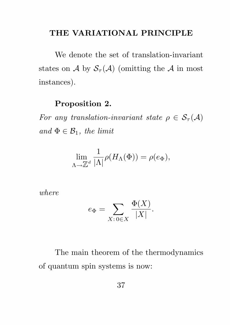
THE VARIATIONAL PRINCIPLE
We denote the set of translation-invariant
states on A by Sτ (A) (omitting the A in most
instances).
Proposition 2.
For any translation-invariant state ρ ∈ Sτ (A)
and Φ ∈ B1, the limit
limΛ→Zd
1|Λ|ρ(HΛ(Φ)) = ρ(eΦ),
where
eΦ =∑
X: 0∈X
Φ(X)|X| .
The main theorem of the thermodynamics
of quantum spin systems is now:
37
Theorem 5. For any potential Φ ∈ B1
and β > 0,
f(Φ, β) = infρ∈Sτ
[ρ(eΦ)− β−1s(ρ)].
Moreover, the infimum is attained at a non-
empty set of points SΦτ (β), which is a closed and
convex subset of Sτ .
If SΦτ (β) contains more than one point for
a given potential Φ and inverse temperature β,
then Φ has a first-order phase transition at
β. The extremal points of SΦτ (β) represent the
pure phases. These are in fact also extremal
translation invariant states.
38
MEAN-FIELD THEORY
Let M be the algebra of all m×m complex
matrices,
AN =N⊗
n=1
M
and
A = ∪∞N=1AN .
Let ρ be a state on M with density matrix
ρ =e−βh
Trace e−βh,
where h ∈ M is hermitian. Define the product
state ωρ = ⊗∞n=1ρ on A. We define the relative
entropy of a state φ on AN by
S(φ, (ωρ)N ) = Trace(φ ln ρ⊗N )− Trace(φ ln φ).
39
As above, the mean relative entropy then exists
for permutation-invariant states φ on A:
Theorem 6. For any permutation-
invariant state φ on A, the mean relative en-
tropy
s(φ, ωρ) = limN→∞
1N
S(φN , (ωρ)N )
exists. Moreover, it has the following proper-
ties:
i. ln λmin ≤ s(φ, ωρ) ≤ 0, where l; ambdamin
is the smallest eigenvalue of ρ;
ii. s(ρ) is an affine upper semicontinuous
function of the state ρ.
40
Given a hermitian x ∈ M, we denote xn a
copy of x in the n-th factor of A. We denote
also
xN =1N
(x1 + . . . + xN ).
Lemma 7. Suppose that φ is a
permutation-invariant state on A and g is a
real-valued polynomial function on R. Then the
limit
eg(φ) = limN→∞
φ(g(xN ))
exists.
This leads to an analogue of the variational
principle for permutation-invariant states:
41
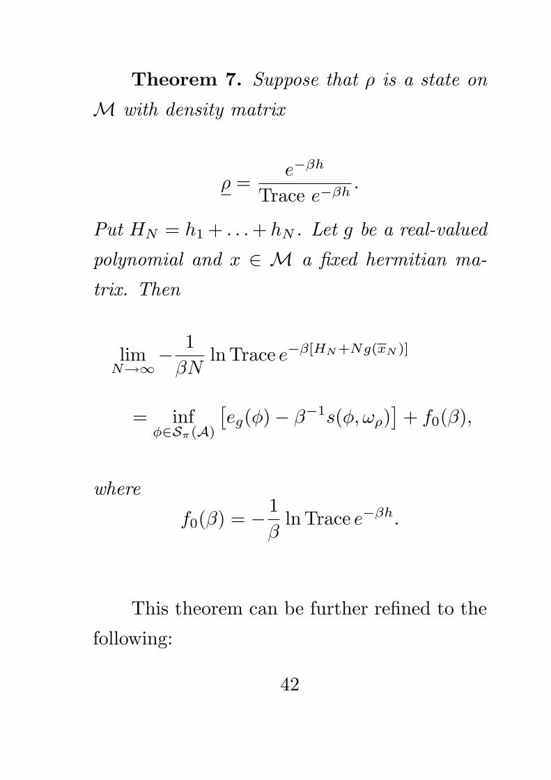
Theorem 7. Suppose that ρ is a state on
M with density matrix
ρ =e−βh
Trace e−βh.
Put HN = h1 + . . . + hN . Let g be a real-valued
polynomial and x ∈ M a fixed hermitian ma-
trix. Then
limN→∞
− 1βN
lnTrace e−β[HN+Ng(xN )]
= infφ∈Sπ(A)
[eg(φ)− β−1s(φ, ωρ)
]+ f0(β),
where
f0(β) = − 1β
ln Trace e−βh.
This theorem can be further refined to the
following:
42
Theorem 8. Suppose that ρ is a state on
M with density matrix
ρ =e−βh
Trace e−βh.
Put HN = h1 + . . . + hN . Let g be a real-valued
polynomial and x ∈ M a fixed hermitian ma-
trix. Then
limN→∞
− 1βN
lnTrace e−β[HN+Ng(xN )]
= infφ∈S(M)
[g(φ(x))− β−1S(φ, ρ)] + f0(β)
= infu∈[−||x||,||x||]
[g(u) + β−1I(u)],
where
I(u) = supt∈R
[tu−G(t)]
43
and
G(t) = ln Trace e−βh+tx.
This theorem is proved using the following
two results:
Theorem 9. (Størmer) The extremal
permutation-invariant states of A are the prod-
uct states. Hence every permutation-invariant
state is a convex combination of product states.
This reduces the expression for the free en-
ergy density to the first expression in Theorem
8. To obtain the second expression, we use the
following lemma:
44
Lemma 8. For any state φ ∈ S(M),
S(φ, ρ) ≤ −I(φ(x)) + βf0(β).
Moreover, if S(φ, ρ) = −I(φ(x)) + βf0(β)
> −∞ and I(z±) = +∞, where
z± = limt→±∞G′(t), then there exists t0 ∈ Rsuch that