Vibrations are mechanical oscillations about an equilibrium position. There are caseswhen vibrations are desirable, such as in certain types of machine tools or productionlines. Most of the time, however, the vibration of mechanical systems is undesirableas it wastes energy, reduces efficiency and may be harmful or even dangerous. Forexample, passenger ride comfort in aircraft or automobiles is greatly affected bythe vibrations caused by outside disturbances, such as aeroelastic effects or roughroad conditions. In other cases, eliminating vibrations may save human lives, a goodexample is the vibration control of civil engineering structures in an earthquake
scenario.All types of vibration control approaches—passive, semi-active and active—requireanalyzingthedynamicsofvibratingsystems.Moreover,allactiveapproaches,such as the model predictive control (MPC) of vibrations considered in this bookrequire simplified mathematical models to function properly. We may acquire suchmathematical models based on a first principle analysis, from FEM models andfrom experimental identification. To introduce the reader into the theoretical basicsof vibration dynamics, this chapter gives a basic account of engineering vibrationanalysis.
Thereare numerousexcellent booksavailable on the topicofanalyzing andsolvingproblems of vibration dynamics. This chapter gives only an outline of the usualproblems encountered in vibration engineering and sets the ground for the upcomingdiscussion. For those seeking a more solid ground in vibration mechanics, worksconcentrating rather on the mechanical view can be very valuable such as the workof de Silva [10] and others [4, 22]. On the other hand, the reader may get a very goodgrip of engineering vibrations from the books discussing active vibration controlsuch as the work of Inman [21] and others [15, 18, 37, 38].
The vibration of a point mass may be a simple phenomenon from the physicalviewpoint. Still, it is important to review the dynamic analysis beyond this phenom-enon, as the vibration of a mass-spring-damper system acts as a basis to understandmore complex systems. A system consisting of one vibrating mass has one naturalfrequency, but in many cases, in a controller it is sufficient to replace a continuous
G. Takács and B. Rohal’-Ilkiv, Model Predictive Vibration Control, 25
structure with complex geometry. The vibration dynamics of point mass and othercomparably simple models may represent a surprisingly large portion of real-lifemechanical systems [8, 21]. We will begin our analysis in the first section with a casein which damping is not considered, then gradually build a more detailed represen-
tation of the physics of vibrations. Section2.2 will introduce damping to the simplevibrating point mass, and following this, Sect.2.3 considers the forced vibration of this essential mechanical system.
Multiple degree of freedom systems will be introduced in Sect.2.4 including aconcise treatment of the eigenvalue problem and modal decomposition. Since vibra-tion dynamics of the continuum is a complex and broad topic, Sect.2.5 will onlymake a brief excursion to distributed parameter systems. The transversal vibrationof cantilever beams will be covered, as in upcoming chapters such a demonstrationsystem will be utilized to test the implementation of model predictive controllers.
Finally, this chapter ends with a discussion on the models used in vibration controlin Sect.2.6. This section covers transfer function models, state-space models, iden-tification from FEM models and experimental identification. The aim of this chapteris to briefly introduce the mathematical description of vibration phenomena, in orderto characterize the nature of the mechanical systems to be controlled by the modelpredictive control strategy presented in the upcoming chapters of this book.
Figure 2.1 illustrates the Venus Express spacecraf t1 under preparation for experi-mental vibration dynamics analysis [12]. The body of the spacecraft is equipped withaccelerometers while outsidedisturbance is supplied to thestructure via a shake table.
Gaining knowledge on the vibration properties of mechanical systems is essentialfor both active and passive vibration engineering, as unexpected vibratory responsemay jeopardize mission critical performance or structural integrity.
2.1 Free Vibration Without Damping
The simplest possible example that may help understand the dynamics of vibrationsis the oscillating point mass, which has one degree of freedom. Such a system is
schematically illustrated in Fig. 2.2. Let us assume for now that damping is negligibleand there is no external force acting on the system. The vibrating mass, often referredto as the simple harmonic oscillator, has a mass of m and is sliding on a frictionlesssurface. The position of the mass is denoted by one time-dependent coordinate, q(t ).
The mass is connected to a surface with a linear spring, having the spring constant k .
According to Newton’s second law of motion, there is an inertial force generatedby the mass, which is proportional to its acceleration [10]:
F m = md 2q
dt 2= mq(t ) (2.1)
1 Courtesy of the European Space Agency (ESA) and European Aeronautic Defence and SpaceCompany (EADS)-Astrium.
Fig. 2.1 Venus Express spacecraft is under preparation for experimental vibration dynamicsanalysis on a shake table [12]
where q(t ) is the acceleration and F m istheinertialforceofthemass.Thereisanotherforce acting against this, which is proportional to the spring constant k [4, 22, 41]:
F k = kq (t ) (2.2)Because there is no other energy source or sink, the sum of these two forces will bezero. We can now assemble our equation of motion, which is an ordinary differentialequation (ODE) given by [4, 10, 21, 49, 51]:
Fig. 2.2 Free vibration of apoint mass without damping
0q t
Mass: m
Spring: k
F k kq t
mq(t ) + kq (t ) = 0 (2.3)
One may classify mechanical vibrations according to whether an outside force ispresent:
• free vibration• forced vibration
In free vibration, a mechanical system is excited by an initial condition, such as adisplacement, velocity or acceleration and then is allowed to vibrate freely withoutfurther force interaction. A mechanical system in free vibration will oscillate withits natural frequency and eventually settle down to zero due to damping effects. Inforced vibration, an external force is supplied to the system.
We may inspect how the moving mass will physically behave by imagining thatwe deflect our spring and move the mass to an initial position of q(0), then let itgo without inducing an initial velocity or acceleration. The mass will start to vibrateback and forth, and since there is no energy dissipation, its position will oscillatebetween q(0) = ±q. Ifweplotitspositioninrelationwithtime,wewillgetharmonicmotion, which can be described by a trigonometric function. If we multiply a sinefunction shifted from zero by φ radians by our amplitude, we have an oscillatingharmonic motion between ±q. In addition to the amplitude, this function has aperiod of oscillations as well. Let us denote the angular frequency by ωn, whichin fact expresses the frequency of oscillations. Now we have a full mathematicaldescription of the assumed motion of the mass [15, 21]:
q(t ) = q sin(ωn t + φ) (2.4)
where t is the progressing time, q is the amplitude and ωn is the angular velocityexpressing the period of the oscillations. The constant amplitude q and phase shiftφ are constants that can be uniquely determined based on the initial conditions. Wecan substitute this trial solution in (2.4) back into the equation of motion in (2.3) and
after double differentiating the first term we will get
−mω2n (q sin(ωn t + φ)) + k (q sin(ωn t + φ)) = 0 (2.6)
we can further simplify this to calculate ωn and get [41, 49]:
ωn =
k
m(2.7)
Substituting this back to the original trial solution (2.4) and using the initialconditions, we get a solution of our ODE. We can convert the angular or circularperiod of vibration ωn expressed in rad/sec into more familiar units [15, 51, 49]:
f n =1
2πωn =
1
2π k
m (2.8)
where f n gives oscillations per second or Hz (Hertz), or [49]
T n = 1
f n= 2π
ωn
= 2π
m
k (2.9)
which gives us the period of one oscillation in seconds.If we divide the equation of motion in (2.3) by the mass, we can express it in
terms of the angular natural frequency ωn:q(t ) + ω2
nq(t ) = 0 (2.10)
The solution in (2.4) is in fact a trial solution, which is a type of educated engi-neering guess;nevertheless if it works then it is the solution itself [21].Inourcase,thetrial solution in Eq. (2.4) works and it is a valid solution of the vibrating point mass.Although it is a product of a logical deduction, there are other ways to express theexpected solution of the ODE describing the equation of motion of the point mass.
A common alternative way to express the displacement of the point mass is to usean exponential function of time. This is a more mathematical representation of thesame concept [21]:
q(t ) = qeκt (2.11)
where q is the complex vibration amplitude. This representation is called the phasor
representation, where a phasor can be simply understood as a rotating vector [15].Note that in the field of vibration mechanics instead of κ the phasor representationuses λ. In order to keep the notation consistent throughout the book, this customhas been changed in order to reserve λ for concepts used in predictive control. Therotation velocity of the vector is included in the complex variable κ, which is essen-tially an eigenvalue. The real part of the amplitude q is the physical amplitude, whilethe real component of the phasor describes the harmonic motion of the point mass.
Substituting the trial solution in (2.11) to the original equation of motion and differ-entiating results the same expressions for ωn , however κ can assume both negativeand positive values. The undamped natural frequency ωn is the positive of the two κ
solutions.
κ = ± j ωnt (2.12)
The reason that e( x ) or the natural exponent is oftenused in vibration analysis insteadof simple trigonometric functions comes from the fact that it is mathematically easierto manipulate the exponential function and solve differential equations by expect-ing solutions in this form. The complex exponential is simply an eigenfunction of differentiation. Although trigonometric functions naturally come to mind whendescribing oscillatory motion, the natural exponential function e( x ) appears com-
monly in trial solutions of ODE describing vibration phenomena. The equivalencebetween trigonometric functions and the exponential function is given by Euler’sformula. The general solution of the equation of motion after substituting (2.11) andsolving for κ will be
q(t ) = Ae− j ωn t + Be j ωn t (2.13)
where A and B are integration constants determined by the initial conditions. Thegeneral solution can be equivalently described by an equation using trigonometricfunctions [4, 22]:
q(t ) = A cos ωnt + B sin ωnt (2.14)
where A and B are again integration constants to be determined based on the initialconditions.
2.2 Free Vibration with Damping
The previous section discussed free vibration of a point mass without damping.This means that a mass connected to a spring and deflected to the initial positionof q(0) = q would oscillate with the same amplitude indefinitely. As we can see,this is a very unrealistic model—we have to add some sort of energy dissipationmechanism, or in other words, damping.
Damping is a complex phenomenon, not very well understood and modeled inscience. Different damping models exist; however, these represent reality only undercertain conditions and assumptions. Probably the most popular damping model is
viscous damping, which expresses the damping force that is proportional to velocityby a constant b. This force can be expressed by [21, 50]:
Fig. 2.3 Free vibration of apoint mass with viscousdamping
0q t
Mass: m
Spring: k
F k kq t
b
F b bq t
We can improve our previous model by adding this damping force to our system.Let us have the same vibrating mass m connected by a spring with the linear spring
constant k to a fixed surface. Displacement is measured by q(t ) and let us adda viscous damper with the constant b to our representation. This is representedschematically by Fig. 2.3.
Now that we know the viscous damping force is expressed by (2.15), we can addit to the original equation of motion. The spring force F k and the damping force F bact against the inertial force F m . The sum of these forces is zero, if we express this,we obtain an ODE again [4, 10, 21, 22]:
mq(t ) + bq(t ) + kq (t ) = 0 (2.16)
Dividing the whole equation of motion by m results in the following term:
q(t ) + b
mq(t ) + k
mq(t ) = 0 (2.17)
Let us call half of the ratio of the viscous damping constant b and mass m as δd
or [49]:
δd =1
2
b
m(2.18)
and use (2.7) to substitute for k /m with yields [51, 52]:
q(t ) + 2δd q(t ) + ω2nq(t ) = 0 (2.19)
Another common representation of the damping both in mechanical vibration analy-sis and vibration control is proportional damping ζ 2 which is expressed as a percent-age of critical damping [18, 51, 52]:
km . Instead of expressing the simpli-fied differential equation in the terms of the damping coefficient δd as in Eq.(2.19)we may express it using proportional damping ζ and get [4, 10, 21]:
q(t ) + 2ζ ωn q(t ) + ω2nq(t ) = 0 (2.21)
Let us now assume that the trial solution to the ODE will come in the form of (2.11). Remember, this is the more mathematical representation of our solution butthe differentiation of an exponential function is the exponential itself which makesthe evaluation process a little simpler. After substituting the trial solution into (2.21)we obtain the following equation:
d 2(eκt )
dt 2
+2ζ ωn
d (eκt )
dt +ω2
n(eκt )
=0 (2.22)
and after differentiating this will be reduced to
κ2 + 2ζ ωnκ + ω2n = 0 (2.23)
Solving this using simple algebra will yield the solution for κ. The roots of thisequation will be [49]:
κ1,2
= −ζ ωn
±ωn ζ 2
−1
= −ζ ωn
±j ωd (2.24)
The damped natural frequency in terms of proportional damping ζ will be then:
ωd = ωn
1 − ζ 2 (2.25)
In this interpretation the overdamped, underdamped and critically damped oscilla-tions are defined by the magnitude of ζ. As ζ is a percentage of critical damping,ζ < 1 will result in an underdamped decaying periodic motion, ζ > 1 will result inan overdamped aperiodic motion, while ζ = 1 will result in a periodic and critically
damped motion. Similarly, by substituting the same trial solution into Eq. (2.19) willyield:
d 2(eκt )
dt 2+ 2δd
d (eκt )
dt + ω2
n(eκt ) = 0 (2.26)
which after differentiation will be reduced to
κ2 + 2δd κ + ω2n = 0 (2.27)
in the terms of δd expressing the amount of damping in the system. The roots κ1,2 of this characteristic equation are expressed by:
The second term is the damped natural frequency ωd or
ωd =
δ2d − ω2
n (2.29)
Depending on the magnitude of the damped natural frequency ωd we may haveoverdamping, critical damping or underdamping. Overdamping is the case, whenthe initial conditions such as initial displacement or velocity result in an aperiodicmotion. From now on we will assume that ζ < 1 or equivalently ω2
d > δ2d which
results in a periodic vibration with a constantly decaying amplitude.Let us now interpret this in the physical sense: we cannot express the solution
as a simple harmonic function anymore. Because of the energy dissipation, for anunderdamped system, the vibration amplitudes will gradually decay and the systemwill settle at equilibrium. We have to introduce an exponential term, to simulate
decay caused by the damping. Our previously assumed solution general solution in(2.4) will be changed to [21]:
q(t ) = qe−ζ ωn t sin(ωd t + φ) (2.30)
The first exponential term e−δd ωn t introduces the exponential decay and emulates thedamping effect. Using trigonometric identities, this can also be written as [22]:
q(t ) = e−ζ ωn t ( A cos(ωd t ) + B sin(ωd t )) (2.31)
where A and B are integration constants which can be determined from the initialconditions. The general solution of the free vibration of the underdamped point masscan also be written in terms of δd by stating that [51, 52]:
q(t ) = qe−δd t sin(ωd t + φ) (2.32)
or equivalently as
q(t ) = e−δd t ( A sin(ωd t ) + B cos(ωd t )) (2.33)
2.3 Forced Vibration of a Point Mass
Thedamped vibration of a pointmass is a passive representation of dynamic systems.Its motion is only controlled by initial conditions such as deflecting the spring into aninitial displacement q(0) or adding an initial velocity q(0) to the vibrating mass. Wehave to introduce an outside force in order to model a controllable active vibratingsystem. Let us assume that—in addition to the spring, damping and inertial forces—an external force f e(t ) can also supply energy to the system. Combining the equationof motion in (2.16) for the damped vibrating point mass with this external force f e(t )
we will get the following new equation of motion incorporating an outside forceeffect, for example an actuator or a disturbance [49]:
Fig. 2.4 Forced vibration of a point mass with viscousdamping
0
f e(t )
q t
Mass: m
Spring: k
F k kq t
b
F b bq t
mq(t ) + bq(t ) + kq (t ) = f e(t ) (2.34)
This is a second order ordinary differential equation, just like in the previous cases.The type of the outside excitation force can be arbitrary and its course may be
mathematically described by a step, impulse, harmonic, random or any other func-tions. To evaluate an analytic solution of the forced equation of motion, we have tohave at least some sort of knowledge about the excitation. Let us therefore assumethat our excitation force is harmonic, generated for example by a rotating imbalanceso we may describe it by [4, 21]:
f e(t ) = ˜ f e sin ω f t (2.35)
where ˜ f e is the amplitude of the excitation force and ω f is the angular frequencyof the outside disturbance. If we substitute this back into our original equation of motion for the forced response of the point mass in (2.34) we will get
mq(t ) + bq(t ) + kq (t ) = ˜ f e sin ω f t (2.36)
It would be natural to assume that, after an initial transient phase, the vibrating pointmass will start to copy the harmonic motion of the outside excitation. This physicalassumption can be translated into an expected trial solution of the time response
given by:q(t ) = qe j (ω f t +φ) (2.37)
where q is the amplitude of our vibrations. Substitute this back into the ODE express-ing the forced response of the point mass in (2.36), differentiate and simplify to getthe amplitude [21]:
q = ˜ f e1
−mω2
f
+j ω f b
+k
(2.38)
This is of course just a solution for one type of external force. This representationlooks much like a transfer function, and in fact, it is easy to apply Laplace transfor-mation to get transfer functions for controller design. For control purposes, it is also
possible to transform our ODE into a decoupled form, which is referred to as thestate-space representation.
Thesolutionoftheequationofmotionconsistsoftwoparts.Thetransientresponsedescribes the passing effects, while the steady-state response will characterize the
response after the initial effects have settled. The total time response of an under-damped system with ζ < 1 will be [21]:
q(t ) = e−ζ ωn t ( A sin ωd t + B cos ωd t ) + q(sin ω f t − φ) (2.39)
which is a sum of the steady state and the transient solution. Note that this generalsolution contains integration constants A and B which in general are not the sameas the ones for free vibration. Furthermore, note the three angular frequencies in thisequation: the angular natural frequency ωn, the damped angular natural frequencyωd and the frequency of the periodic excitation ωn.
The analytic solution for other types of excitation is analogous to the periodiccase. As this work is interested rather in the control aspects of (forced) vibrations,tools known from control engineering such as transfer function and state-space rep-resentations will be used to evaluate the response of a system to an outside excitation.To those interested in more details on the analytic representation of forced vibrationsthe books by de Silva [10] and others [4, 22] may be recommended.
2.4 Multiple Degree of Freedom Systems
The very simple single degree of freedom mass-spring-damper system introduced inthe previous sections gives a good foundation for the analysis of vibrating systems.It is possible to simplify the essential dynamic behavior of many real mechanical sys-tems to SDOF and replace it with an analysis procedure similar to the one introducedpreviously [8, 21].
In the vibration analysis of mechanical systems with multiple degrees of freedom(MDOF), instead of one vibrating mass, we replace our real structure with two or
moreoscillatingmasses. If the real systemhaswell-definedseparatemoving parts, wecan consider it as a lumped interconnected parameter system. The degreesof freedomof a lumpedparameter system are equal to the number of vibrating mass points andthis is also true for the number of resonant frequencies. A mechanical system orstructure which does not have well-defined separately oscillating parts but consistsof a continuously spread mass and geometry is a distributed system. Continuum ordistributed parameter systems have an infinite amount of resonant frequencies andcorresponding vibration shapes. It is, however, possible to discretize the system intolarge amounts of lumped interconnected parameters and approximate its behaviorwith methods commonly used for lumped parameter systems. This idea is in factused in FEM software to extract the vibration dynamics of distributed mechanicalsystems defined with complex three-dimensional geometry.
Let us choose a very simple example, which has more than one degree of freedomand therefore may be considered as a MDOF system. The system of connected
Fig. 2.5 Multiple degrees of freedom system: connected set of two masses
moving masses illustrated in Fig. 2.5 is sliding on a frictionless surface. Now insteadof one coordinate defining the movement, we have two for each moving mass: q1(t )
and q2(t ). The two moving masses m1 and m2 are connected to each other and
the surrounding fixed wall through a series of springs and dampers with the springand damping coefficients k 1, k 2, k 3 and b1, b2, b3. There are external force inputsassociated with individual masses denoted by f e1 and f e2 .
Using a simple mechanical analysis, we may create a free body diagram foreach mass and analyze the forces acting on them. After assembling the equations of motion, we obtain the following set of equations for our two masses [4, 10, 18]:
m1q1 + (b1 + b2)q1 − b2q2 + (k 1 + k 2)q1 − k 2q2 = f 1 (2.40)
m2
¨q2
−b2
˙q1
+(b2
+b3)
˙q2
−k 2q1
+(k 2
+k 3)q2
=f 2 (2.41)
It is possible to rewrite the one equation for motion per moving mass into a compactset, using matrix notation [10, 37, 52]:
m1 00 m2
q1
q2
+
b1 + b2 −b2
−b2 b2 + b3
q1
q2
+
k 1 + k 2 −k 2−k 2 k 2 + k 3
q1q2
=
f e1 f e2
(2.42)
Note the similarity between this equation of motion and the SDOF forced equationmotion in (2.34). We have a matrix containing the masses, which is multiplied bya vector of accelerations. Similarly, we have matrices containing damping elementsand spring constants. We can in fact use a matrix notation to create from this [ 21]:
Mq + Bdq + Ksq = f e (2.43)
where matrix M is the mass matrix,3 Bd is the structural damping matrix and Ks isthe stiffness matrix. Vector q contains the displacement coordinates for each degreeof freedom. For an N degree of freedom system the constant matrices M, Bd and Ks
will all have N × N elements.
3 It is customary to denote the mass matrix with M however in the upcoming chapter this symbolwill be reserved for an entirely different concept.
The solution of such systems is in fact very similar to the solution of SDOFsystems. To illustrate this, let us consider a case without damping and with no outsideforce. Removing these effects from the equation of motion in matrix from (2.43),we get [38]:
Mq + Ksq = 0 (2.44)
for which we have to find a solution. Similar to the SDOF systems, our solution canbe expected in a form of a set of harmonic functions, which mathematically is simplyan amplitude multiplied by a complex exponential:
q = qe j ωn t = qeκt (2.45)
As introduced previously, the term e j ωn t
or analogously eκ t
is just a mathematicaltrick tosolve differentialequations byusing the so-called phasor formfor thesolution.If we take the real part of Euler’s formula, we essentially expect a cosine function.Let us substitute this solution to our matrix equation of motion, and differentiateto get:
−ω2
nM + Ks
qe j ωn t = 0 (2.46)
2.4.1 The Eigenvalue Problem
To solve the equation expressed by (2.46) we can assume that the exponential parte j ωt cannot be zero, therefore we will reduce our expression to [37, 38]:
−ωn
2M + Ks
q = 0 (2.47)
This is a problem often encountered in mathematics, called the eigenvalue problem
which in general mathematics assumes the form [22]:
(A − κI) δ = 0 (2.48)
where κ contains the eigenvalues of the system while δ is the eigenvector. To get ourproblem (2.47) into a similar form, we have to multiply it by the inverse of the massmatrix M−1 to get
The solution to the eigenvalue problem expressed by our physical vibrating sys-tem is a set of N eigenvalues ranging from ω2
1, ω22 . . . ω2
N , where N is the numberof degrees of freedom. These eigenvalues have a very well-defined physical mean-ing: they contain the (square of the) angular natural frequencies associated with the
individual masses. Substituting these eigenvalues back into the original equation,we get a set of amplitudes q called the eigenvectors. Each eigenvalue or natural fre-quency has an associated eigenvector. This eigenvector expresses the mode shapesof the system, in other words, the geometrical shape of the vibration within a givenresonant frequency. The magnitude of the eigenvectors is not expressed in physi-cal coordinates—instead, modal shapes are scaled by a method of choice. To avoidconfusion, we will substitute the notation qi with δi referring to the fact that theseamplitudes have a physically valid magnitude only in relation to each other but notglobally.
Eigenvalues and eigenvectors expressing the angular natural vibration frequencyof individualmasses andthevectorsof modal shapeassociated with those frequenciescan be assembled in a compact notation:
Λ = diag(ω2i ) = diag(κi ) =
⎡⎢⎣
ω21 · · · 0
.... . .
...
0 · · · ω2 N
⎤⎥⎦ =
⎡⎢⎣
κ1 · · · 0...
. . ....
0 · · · κ N
⎤⎥⎦ (2.51)
Δ = δ1 δ2 δ3 . . . δ N
= q1 q2 q3 . . . q N
(2.52)
where Λ is a diagonal matrix with the square of the individual eigenfrequencies ω2i
on its main diagonal. Solving theeigenvalue problem, we get the modal shapes whichare expressed by the amplitudes δi associated with the eigenfrequencies.
2.4.2 Modal Decomposition
Itispossibletosimplifythesolutionofamulti-degreefreedomsystembysubstitutingit with a set of single degree freedom systems. Eigenvectors have a mathematicalproperty called orthogonality, which is the basis of this simplification. If Δ is theset of eigenvectors, it can be shown that when we use it to multiply the mass matrixfrom both sides we obtain [22, 38, 52]:
while multiplying the stiffness matrix by Δ from both sides we get
ΔT KsΔ =
δ1 δ2 δ3 . . . δ N
T
Ks [δ1δ2δ3 . . . δ N ]
=⎡⎢⎢⎢⎣
δT
1K
sδ
1δT
1K
sδ
2. . . δT
1K
sδ
N δT
2 Ksδ1 δT 2 Ksδ2 . . . δT
2 Ksδ N
.... . . . . .
...
δT N Ksδ1 δT
N Ksδ2 . . . δT N Ksδ N
⎤⎥⎥⎥⎦ = Λ(2.54)
Keeping in mind the orthogonality properties of the modal matrices, we can intro-duce a coordinate transformation, which changes the original displacement coordi-nates into the so-called modal coordinates or modal participation factors:
q = Δξ (2.55)
This transformation may be interpreted in a way that we take the vibration amplitudeinphysicalcoordinatesasalinearsumofmodalshapes.Thecoordinateξ isalsocalledthe modal participation factor, because it determines how each mode participates inthe final vibration. Mathematically this is:
q = ξ 1δ1 + ξ 2δ2 + ξ 3δ3 + · · · + ξ i δi + · · · + ξ N δ N (2.56)
We can use (2.55) substitute for q in the matrix equation of motion for free,undamped systems to get [22, 38]:
MΔξ + KsΔξ = 0 (2.57)
Let us now multiply the equation by ΔT from the left to get
ΔT MΔξ + ΔT KsΔξ = 0 (2.58)
Using the orthogonality properties introduced in (2.53) and (2.54) we can simplify
this equation to get
ξ + Λξ = 0 (2.59)
Instead of having a large coupled multiple degree of freedom, this decomposes theoriginal system into a set of several single degree of freedom systems [22]:
ξ i + ω2i ξ i = 0 (2.60)
where ξ i
are the individual modalparticipation factors associated with thegiven massmi and ωi is the angular natural frequency.
Solutionsforthefreeandforcedvibrationforbothdampedandundampedsystemscan be developed using similar methods.
In practice, the vibration of continuously distributed parameter systems is solved andanalyzedthroughthefiniteelementmethod.Asinthecaseofotherfieldsofscience,inFEM vibration analysis the continuous structure and its geometry are discretized intofinite portions, the elements.Thecontinuouslydistributedstructureisthenconsidereda large lumped parameter system with hundreds, thousands and even millions of degrees of freedom. If one aims to perform a modal analysis on a continuous systemwith complex geometry, the FEM software first creates a discretized version of theoriginal structure. The equation of motion is then expressed in the matrix form of (2.43) and then the eigenvalue problem is solved. The solution of the eigenvalueproblem with large matrices is not a trivial task, fortunately numerical mathematicshave provided us with tools to speed up this process.
2.5.1 Exact Solution
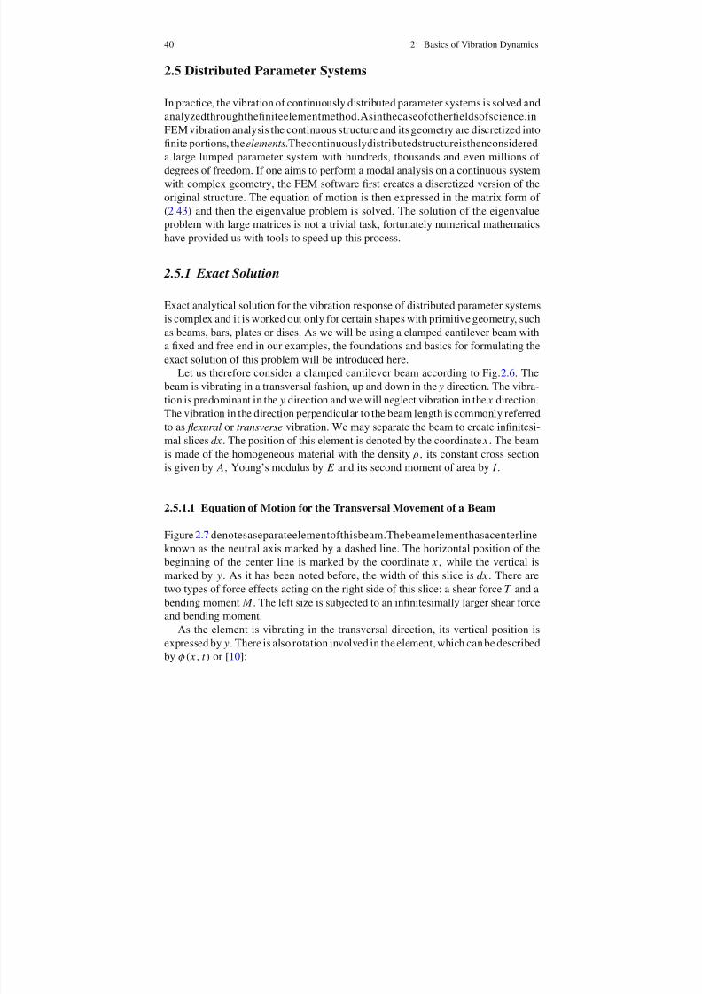
Exact analytical solution for the vibration response of distributed parameter systemsis complex and it is worked out only for certain shapes with primitive geometry, suchas beams, bars, plates or discs. As we will be using a clamped cantilever beam witha fixed and free end in our examples, the foundations and basics for formulating theexact solution of this problem will be introduced here.
Let us therefore consider a clamped cantilever beam according to Fig. 2.6. Thebeam is vibrating in a transversal fashion, up and down in the y direction. The vibra-tion is predominant in the y direction and we will neglect vibration in the x direction.The vibration in the direction perpendicular to the beam length is commonly referredto as flexural or transverse vibration. We may separate the beam to create infinitesi-mal slices dx . The position of this element is denoted by the coordinate x . The beamis made of the homogeneous material with the density ρ , its constant cross sectionis given by A, Young’s modulus by E and its second moment of area by I .
2.5.1.1 Equation of Motion for the Transversal Movement of a Beam
Figure 2.7 denotesaseparateelementofthisbeam.Thebeamelementhasacenterlineknown as the neutral axis marked by a dashed line. The horizontal position of thebeginning of the center line is marked by the coordinate x , while the vertical ismarked by y. As it has been noted before, the width of this slice is dx . There aretwo types of force effects acting on the right side of this slice: a shear force T and abending moment M . The left size is subjected to an infinitesimally larger shear force
and bending moment.As the element is vibrating in the transversal direction, its vertical position isexpressed by y. There is also rotation involved in theelement,which canbe describedby φ ( x , t ) or [10]:
Fig. 2.6 Schematicrepresentation of a clampedbeam under transversalvibration
x dx
y
0
Fig. 2.7 Forces andmoments acting on theinfinitesimally small portionof the clamped beam undertransversal vibration
x
dx
y
0
M
T
M ∂ M ∂ x
dx
T ∂ T ∂ x
dx
θ ( x , t ) = d y( x , t )
d x (2.61)
therefore both the position of the element and its rotation is expressed by just onecoordinate and its derivativewith respect to x . Let us now express the second momentof inertia I of the element d x defined in the plane perpendicular to the direction of the transversal motion using the polar moment of inertia defined at the neutral axis:
I = ρ J (2.62)
If we look at the forces and moments acting on the element, we can write theequation of motion for the beam as [22, 10, 51, 52]:
ρ A∂2 y( x , t )
∂t 2= −T + T + ∂ T
∂ x d x (2.63)
ρ J ∂2
∂t 2∂ y( x , t )
∂ x =
T d x
2 + M
+ T +
∂ T
∂ x d x d x
2 − M
−∂ M
∂ x d x (2.64)
where the first equation describes the effects of the shear force T and the secondequation describes the moment effects. If we take a close look at the first equation,the term on the left is nothing more than the mass of the element (ρ A) multiplied bythe transversal acceleration expressed as the second derivative of the y coordinate,thus creating an inertial force. The right side of the equation is merely a sum of shearforces acting on both sides of this element. The second equation is very similar, withthe inertial moment on the left and the sum of all moments acting on the elements
on the right.We may discard some of the second order terms that do not contribute to thesolution significantly and after rearranging the equations we finally get [21, 52]:
It is possible to collect these two equations into one, by expressing T from the secondequation (2.66) and substituting it back into the first one after differentiation. We willget one equation of motion given by
ρ A∂2 y( x , t )
∂t 2= ∂2 M
∂ x 2+ ρ J
∂
∂ x ∂3 y( x , t )
∂t 2∂ x (2.67)
In statics, the curvature r of the deflection curve marked by the dotted line in themiddle of Fig. 2.7 can be expressed by:
1
r ≈ d 2 y
d x 2= − M
E J (2.68)
We can express M from this and substitute it back into our simplified equation of motion in (2.67) so we get [22]:
ρ A ∂2 y( x , t )∂t 2
= − E J ∂2∂ x 2
∂2 y( x , t )
∂t 2
+ ρ J ∂
∂ x
∂3 y( x , t )
∂t 2∂ x
(2.69)
This is the equation of motion for a beam vibrating in the transversal direction.To simplify notation, let us mark the time differentiation of y( x , t ) with respect to t
by dots as in ˙ y and the position differentiation with respect to x by Roman numeralsas in yii . If we ignore the effects of rotational inertia, we may denote the simplifiedequation motion for the free transversal vibration of a beam with constant crosssection by [4, 52]:
ρ A ¨ y + E J yiv = 0 (2.70)
We may further simplify this by dividing the whole equation by ρ A and introducing
c = E J
ρ A(2.71)
where c is a constant4 encompassing the square of the longitudinal wave and thesquare of the radius of quadratic moment of inertia. We finally arrive at the following
equation of motion [3, 10, 21]:
4 Certain literature divides this constant to a c = c20i2, where c0 = E
ρis the speed of the
longitudinal wave and i is the radius of quadratic moment of inertia given by i = J A
This equation expresses the free transversal vibration of a beam, neglecting thedynamic effects of the longitudinal forces and rotational inertia. Clearly, there is a
lot of simplification assumed in this representation. If the above equation of motionwould also include the effects of the rotational inertia, it would be according toRayleigh’s beam theorem. On the other hand, if it would include both the effectsof the rotational inertia and the longitudinal forces, it would be Timoshenko’s beamtheorem[52].TheequationpresentedhereisthusaspecialversionoftheTimoshenkobeam theory also called the Euler–Bernoulli beam equation—or the classical beamtheory.
2.5.1.3 Solving the Equation of Motion
The equation of motion in (2.72) merely gives a simplified representation of beamdynamics. The solution depends on the problem, as we also have to introduce bound-ary conditions and initial conditions. As the position differentiation of y is of thefourth degree, we can have four types of boundary conditions at the beginning andat the end [51]:
y(0, t ) = Ξ 1(t ) y(l, t ) = Ξ 5(t )
yi
(0, t ) = Ξ 2(t ) yi
(l, t ) = Ξ 6(t ) yi i (0, t ) = Ξ 3(t ) yi i (l, t ) = Ξ 7(t )
yii i (0, t ) = Ξ 4(t ) yii i (l, t ) = Ξ 8(t )
(2.73)
These boundary conditions express the position of the beam (and its derivatives) atany given time. In more practical terms, the zeroth derivation is a deflection position,while the first is the angle of the tangent line to the neutral axis. Moreover, the secondand third derivatives can be expressed using the moment and shear force as:
yii (0, t ) = − M
E J (2.74)
yi i i (0, t ) = − T
E J (2.75)
In addition to the boundary condition, we also have initial conditions, expressinggeometrical configuration at zero time:
y( x , 0)=
Ψ 1
( x )˙
y( x , 0)=
Ψ 2
( x ) (2.76)
As our main interest is vibration dynamics, let us assume that we want to find theresonant frequencies and mode shapes of a beam under free transversal vibration.Furthermore, let us now expect to arrive at a solution in the following form [21, 22]:
meaning that the position at a given place and time is composed of a combination of function a( x ), which is only dependent on the horizontal position and V (t ) which
is only dependent on time. We may substitute this expected form back to (2.72) andget a new equation of motion:
aiv
a= −c
V
V (2.78)
Since the right-hand side of the equation is only a function of time and the left-handside of the equation is only the function of position x , each side of the equation mustbe equal to a constant. Let us call this constant Ω2, which will help us separate the
partial differential equation in (2.78) into two ordinary differential equations [22]:
ai v − Ω2
ca = 0 (2.79)
V + Ω2V = 0 (2.80)
In order to keep the notation simple, let us introduce the new constant υ4 as:
υ4 = Ω
2
c (2.81)
NowwecanexpectthesolutionofEq. (2.79) inthefollowingform,withaconstant A and an exponential term:
a( x ) = Aer x (2.82)
Substituting this back into (2.79) will yield a characteristic equation with the follow-ing roots:
r 1,2 = ±υ r 3,4 = ± j υ (2.83)
The solution of (2.79) will now assume the form [10, 22]:
a( x ) = A1eυ x + A2e−υ x + A3e j υ x + A3e− j υ x (2.84)
Utilizingthewell-knownEuler’sformulaestablishingarelationshipbetweentrigono-metric and complex exponential functions
and substituting this back into (2.84) we will get the solution in the following form[4, 10]:
a( x )
=C 1 cosh υ x
+C 2 sinh υ x
+C 3 cos υ x
+C 4 sin υ x (2.87)
Constants C 1, C 2, C 3 and C 4 are integration constants and can be uniquely deter-mined from the boundary conditions.
As different beam setups have different boundary conditions, we will pick aclamped cantilever beam, which is fixed at one end and free to vibrate at the other,as an example. For this clamped cantilever beam, the boundary conditions are givenby [10, 21]:
y(0, t ) = 0 yii (l, t ) = 0
yi (0, t ) = 0 yi ii (l, t ) = 0(2.88)
or, in other words, the beam cannot move at the clamped end and there are no shearforces or moments at the free end. Substituting theseboundary conditions into (2.87),we will get a set of equations for the integration constants [51, 52]:
C 1 + C 3 = 0 (2.89)
υ(C 2 + C 4) = 0 (2.90)
υ2(C 1 cosh υ x + C 2 sinh υ x − C 3 cos υ x − C 3 sin υ x ) = 0 (2.91)
υ2(C 1 cosh υ x + C 2 sinh υ x + C 3 cos υ x − C 3 sin υ x ) = 0 (2.92)
where l is the overall length of the beam implied by the boundary conditions. More-over, for a nonzero υ the first two equations also imply that
C 3 = −C 1 C 4 = C 2 (2.94)
Substituting for C 3 and C 4 in the remaining two equations yields a set of two homo-geneous equations with C 1 and C 2 as unknowns:
(cosh υl + cos υl)C 1 + (sinh υl + sin υl)C 2 = 0 (2.95)
(sinh υl − sin υl)C 1 + (cosh υl + cos υl)C 2 = 0 (2.96)
In order for Eq.(2.95) to have nontrivial solutions, its determinant has to equal zero[21, 51]. Computing this will yield the following frequency equation [21]:
cos υl cosh υl + 1 = 0 (2.97)
Theresonantfrequenciesofthebeamcanbecalculatedbasedon(2.81)bycomputingthe roots of (2.97) and substituting into [22]:
The equations given by (2.89) will not make it possible to compute the integratingconstants,thoughitispossibletocomputetheirratiosandsubstituteitbackinto( 2.87)to get an( x ). The general solution describing the mode shapes of vibration will befinally given by [22, 52]:
y( x , t ) =∞
n=1
( An cos Ωn t + Bn sin Ωnt )an x (2.99)
where the integration constants An and Bn are given by
An = 2l
l
0Ψ 1( x )an ( x )d x (2.100)
Bn = 2
lΩn
l
0Ψ 2( x )an ( x )d x (2.101)
The process of obtaining the resonant frequency and mode shapes for other typesof distributed parameter systems with simple geometry is analogous to the aboveintroduced process. The interested reader is kindly referred to works discussing this
topic in more depth [10, 21]. It is easy to see that working out a solution is a fairlytime-consuming and complicated process, even for systems with simple geometry.This is why most practitionersprefer to utilize finiteelement analysisor experimentalprocedures to assess the vibration properties of such systems.
2.5.2 Damping in Distributed Systems Simulated by FEA
The damping of distributed mechanical systems is a very complex phenomenon.Unfortunately, energy dissipation in materials is not entirely explored by scienceat present. One of the simplest methods to approximate damping is to use theso-calledRayleighdampingwhichisoftenutilizedinFEMsimulations.Thisinvolvescalculatingthedampingmatrixasasumofthemassandstiffnessmatrices,multipliedby the damping constants α and β:
Bd = αM + βKs (2.102)
The damping constants α and β are not known directly, instead they are calculatedfrom the modal damping ratios ζ i . This is actually the ratio of actual damping tocritical damping for a particular mode of vibration. In case ωi is the natural circularfrequency for a given mode of vibration, we can calculate the constants utilizing[51, 52]:
It is often assumed that α and β are constant over a range of frequencies. For a given
ζ i and a frequency range, two simultaneous equations may be solved to obtain theRayleigh damping constants. In most real-life structural applications mass dampingcan be neglected, therefore setting constant α = 0. In these cases, β may be evaluatedfrom the known values of ζ i and ωi:
β = 2ζ i
ωi
(2.104)
2.6 Creating Models for Vibration Control
Different control systems call for different models and representations. There arenumerous popular methods suitable to create a mathematical representation of thereal system such as transfer functions or the state-space representation. We maychoose to begin with a completely analytical fashion, and build our model based onthe exact underlying physics. A mathematical model created on such first principlemodels using the underlying physics and equations is known as a white-box model.Models of vibrating structures are derived on a phenomenological basis for example
in [26, 36, 48].Active vibration control often utilizes advanced materials bonded into thestructure. Moreover, the materials can have a coupled nature, having an intenseelectromechanical interaction with the structure—for example piezoceramics. If theunderlying model is too complicated or it is too formidable to create a first principlesmodel we may use experimental identification. If one is aware of the structure of the underlying physics, they may choose a given model and fit its parameters on anexperimental measurement. This is known as a grey-box model. If nothing is knownabout the physics or one does not choose a model with a fixed structure, black-box
identification is carried out.In active vibration control there is an outside energy source acting on our vibrat-ing mechanical system, such as a piezoelectric actuator. The model representingthe behavior of the system therefore must represent forced vibration, regardless of whether it is created based on first principles or experimental methods.
2.6.1 Transfer Function Models
We will introduce a transfer function representation based on the dynamics analysispresented previously in Sect.2.3 on the forced vibration of a point mass. Recall thatthe equation of motion of a point mass system with damping and a generic outsideforce is
Now in order to create a transfer function from this, we must apply Laplace trans-formation to our equation. Let us denote the Laplace operator with s. The position
coordinate q(t ) will be now denoted instead with Q(s) and our external force f et with F e(s). Differentiation in the Laplace domain is simply multiplication with theLaplace operator, therefore we will get [22]:
ms2 Q(s) + bs Q(s) + k Q(s) = F e(s) (2.106)
The transfer function H (s) will be simply a ratio of the Laplace transform of theoutput divided by the Laplace transform of the input. In this case, we may state thatour transfer function expressing the effect to a force input is simply
H (s) = L {q(t )}L { f e(t )} = Q(s)
F e(s)= 1
ms2 + bs + k (2.107)
In theLaplace domain, we cancompute theoutput of themass-spring-damper systemby the linear combination of the transfer function and an arbitrary force signal byevaluating
Q(s) = H (s)F (s) (2.108)
Another valid representation of the transfer function is given in the term of thenaturalfrequency ωn and the proportional damping ζ [18]. For this, we divide the transferfunction in (2.107) by the mass to get
H (s) =1m
s2 + 2ζ ωn s + ω2n
(2.109)
where c/m = 2ζ ωn and ζ is proportional damping given as a percentage of criticaldamping.
2.6.1.1 Multiple DOF Transfer Functions
Lumped parameter systems with several vibrating masses or equivalent representa-tions of distributed systems can be expressed using a transfer function representationas well. Let us consider a matrix representation of the forced equation of motion foran N degrees of freedom system as in (2.43) and perform a Laplace transform onthe equation in the following sense:
Ms2Q + Bds2Q + KsQ = Fe (2.110)
where sQ denotes an n elements long vector of Laplace operators and output dis-placements, s2Q expresses the elementwise square of the Laplace operators multi-
pliedbytheoutputdisplacementsQ5 intheLaplacedomain.Afterthetransformationand rearranging the terms, the equation of motion will be given in a matrix form inthe s-domain:
H (s)Q = Fe (2.111)
where H (s) is a matrix of partial dynamics contributions. To get the transfer func-tion for particular input and output points, one must rearrange this term. It is highlyrecommended to use computer symbolic algebra to arrive at the final transfer func-tions given large systems with many DOFs [18]. The transfer function representationof systems with several inputs or outputs (MIMO, SIMO, MISO) is not common,most engineering practitioners prefer to use the state-space representation to modelthe behavior of more complex systems.
2.6.1.2 Poles and Zeros
From a controlviewpoint, wemay furtheranalyze thetransferfunction representationin (2.109), to see where the poles and zeros of lightly damped systems are located andwhat the physical interpretation of the poles and zeros of the transfer functions is.For this, let us assume that the proportional damping is approaching zero ζ → 0 toget
H (s) = 1m
s2 + ω2n
(2.112)
As it is usual in control, the denominator of the transfer function is extremely impor-tant.Bysettingthedenominatorequaltozero,wewillgetthecharacteristic equation.The roots of this equation are the so-called poles of transfer function, which amongstothers affect the dynamic behavior and stability of the system. The poles representthe resonant frequencies of the vibrating system, in other words, the frequency valuesat which the inputs will be amplified. The characteristic equation of the vibrating
point mass is
s2 + ω2n = 0 (2.113)
from which we may calculate the poles
s = ± j ωn (2.114)
It is clear that the poles of an undamped system will be located only on the imaginaryaxis (no real part) on complex plane. Similarly, the poles for a lightly damped sys-
tem will be located close to the imaginary axis with very small negative real parts.
5 In order to avoid confusion with Q used in later chapters as input penalty, the multiple DOFdisplacements transformed into the Laplace domain are denoted as Q here.
Fig. 2.8 Location of thepoles for the vibrating pointmass system depending onthe amountof damping
UnstableStable
Im
Re
Increased damping
0
0
Vibrating mechanical systems are inherently open-loop stable, therefore the poles of
the transfer function must have negative real parts. Poles, and therefore the resonantfrequency of a system, only depend on thedistributionof mass, damping and stiffnessand are independent on the excitation point or the measurement of the output [18].
Setting the numerator of a transfer function equal to zero and calculating rootswill yield the zeros of the system. Zeros of the transfer function do depend on thepoint and type of excitation and the output. Some transfer functions may not evenhave zeros. In a physical interpretation, at zeros the vibrating system will attenuatethe input. Similar to the poles, the zeros would also have no real part in the absenceof damping. A pair of poles located at zero indicates a so-called rigid body mode
[18]. A rigid body mode is the case when in the presence of a static or low frequencyoutside force the whole mechanical system moves without moving the parts relativeto each other. In the case of the two vibrating masses example presented earlier inFig. 2.5 a rigid body mode would occur if none of the masses were connected toa ground, but just to each other. At low frequencies or quasi-static forces, the twomasses would move as one without considering the spring and damper in betweenthem.
The location of the poles in the complex plane for the continuous transfer functionof a simple second order vibrating system is demonstrated in Fig. 2.8. The left half of the plane is stable; this is where open-loop physical vibrating system poles are
located.Withoutdamping,thepolesareontheimaginaryaxis,onthevergeofstability(right ). Lightly damped systems have poles very close to the imaginary axis (middle)while a more considerable amount of proportional damping would place the polesfurther away (left ). Generally speaking, this is also true for the zeros of the system.The poles tend to be further away from each other in a lightly damped system, whileincreasing damping values will bring them closer together in the direction of theimaginary axis.
2.6.1.3 Discrete Transfer Functions
As digital control systems work in a sampled fashion instead of a continuous-timetransfer function, we often need to use a discrete transfer function. In a discrete-time
system, the transfer function is created using the Z-transform, which is an analogyto the Laplace transform. For our case, a discrete time transfer function would bedefined by:
H ( z) = Z {q(kT )}Z { f e(kT )} = Q( z)
F e( z)(2.115)
A continuous time transfer function may be converted into discrete time using var-ious algorithms using zero or first order hold to extract the function values in the timedomain. The definition of the Z-transform essentially sums the pairs of the functionvalues multiplied by a corresponding delay operator z−k . Numerous numerical algo-rithms implement this procedure very effectively. Another example of converting acontinuous transfer function into discrete is the so-called bilinear transformation.
If T is the sampling time, to convert from continuous into discrete known as theTustin transformation we can use: A continuous time transfer function may be con-verted into discrete time using various algorithms using zero or first order hold toextract the function values in the time domain. The definition of the Z-transformessentially sums the pairs of the function values multiplied by a corresponding delayoperator z−k . Numerous numerical algorithms implement this procedure very effec-tively. Another example of converting a continuous transfer function into discreteis the so-called bilinear transformation. If T is the sampling time, to convert fromcontinuous into discrete known as the Tustin transformation we can use:
s = 2T
z − 1 z + 1
(2.116)
while the reverse operation into convert from discrete to continuous is
z = 2 + sT
2 − sT (2.117)
Software tools such as for example Matlab also aid the conversion between con-tinuous and discrete time models. In Matlab, this can be carried out using the c2d
command.A transfer function representation can be used to design or tune a controller for the
vibrating system. A common approach used in practice is to utilize a software toolsuch as Matlab or Simulink to simulate the response of a system and the controller.
2.6.1.4 Experimental Identification
We may create a transfer function following a dynamical analysis and fill in the
parameters such as m, b and k from direct measurements and consider them asphysical quantities. However, in experimental identification, we may choose a givengeneric form of a transfer function and not expect to use parameters, which have aphysical sense. Instead, we can use system identification algorithms, which compute
these parameters so that a test signal input matches a measured output. This makessense for example when we would like to replace the dynamics of a continuousclamped beam with a single mass-spring-damper model. We cannot directly measurethese quantities, rather we should find a generic second order transfer function that
properly describes the first resonant mode and is given by
H (s) = L {q(t )}L { f e(t )} = Q(s)
F e(s)= 1
a1s2 + a2s + a3(2.118)
where parameters a1, a2 and a3 are found experimentally using an identificationalgorithm.
2.6.1.5 State-Space Representation
A state-space representation of a dynamic system may be perceived as a wayto decouple high order differential equations into simpler low order equivalents,collected in a matrix representation. The set of first order differential equations thenrelates the inputs and outputs of a system by the aid of an intermediate variablecalled the state. If for example a single DOF vibrating system is described by a sec-ondorderdifferential equation, we may use a state-space equivalent consisting of twofirst order differential equations. Analogously, if an MDOF vibrating system has itsmodes decomposed according to the guidelines presented previously in Sect.2.4.2,
then the behavior of each mode is described by N second order differential equations,which may be changed into 2 N first order equations in the state-space representation.Most modern optimization-based control algorithms such as MPC utilize this typeof mathematical model, and the numerical simulation of time responses is more con-venient as well. To demonstrate the state-space representation of dynamic systems,we may divide the second order differential equation describing the forced responseof the spring-mass-damper system in (2.34) into two first order ones.
2.6.1.6 State-Space Representation for a Single DOF System
Let us begin the rewriting of our second order differential equation by leaving theinertial force at the left side of our equation of motion (2.34) and moving the rest tothe right which will result in:
mq(t ) = −bq(t ) − kq (t ) + f e (2.119)
while dividing the whole by m is
q(t ) = − bm
q(t ) − k m
q(t ) + 1m
f e (2.120)
Because our original ODE is second order, let us choose two new variables x 1(t )
and x 2(t ). These two variables are the so-called state variables and we may combine
themtocreateacolumnstatevector x(t ) .Wemayalsochoosethat x 1(t ) is equivalentto our original position variable q, while x 2(t ) is simply a differentiation of it.
x(t )= x 1(t )
x 2(t ) = q(t )
q(t ) (2.121)
Let us now write a set of two first order ordinary differential equations with the helpof our state variables x 1(t ) and x 2(t ). Substitute these into the transformed equationof motion and simply state that ˙ x 1(t ) = x 2(t ) [5]:
˙ x 1(t ) = x 2(t ) (2.122)
˙ x 2(t ) = − b
m x 2(t ) − k
m x 1(t ) + 1
m f e (2.123)
which can be equivalently written in the following matrix form [5, 10]: ˙ x 1(t )
˙ x 2(t )
=
0 1− b
m− k
m
x 1(t )
x 2(t )
+
01m
0 f e
(2.124)
We may use a more compact matrix notation for the state-space variables x(t );moreover, let us define an input vector u(t ) which contains the outside excitationforce f e as its first element: u =
f e 0
. According to this, the matrix form of the
state-space equation can be written as follows [5, 10]:
x(t ) = Ax(t ) + Bu(t ) (2.125)
y(t ) = Cx(t ) (2.126)
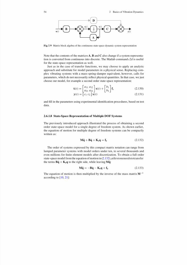
where A is the state transition matrix, B is the input matrix and C is the output matrix.Figure 2.9 illustrates the matrix block algebra of the continuous state-space dynamicsystem representation. The output vector y(t) may contain both the position andvelocity elements of the state or one of them according to the output matrix C. Forexampleavalidchoiceof C is C
= 1 0 whichwouldresultinascalardisplacement
output.
y(t ) = q(t ) = 1 0
x(t ) =
1 0 x 1(t )
x 2(t )
=
1 0 q(t )
q(t )
(2.127)
2.6.1.7 Discrete State-Space Representation
In the discrete time equivalent of the state-space equation we replace the continuous
time variable t by its sampled analogy t = kT , where T is the sample time:
Fig. 2.9 Matrix block algebra of the continuous state-space dynamic system representation
Note that the contents of the matrices A, B and C also change if a system representa-tion is converted from continuous into discrete. The Matlab command c2d is usefulfor the state-space representation as well.
Just as in the case of transfer functions, we may choose to apply an analyticapproach and substitute for model parameters in a physical sense. Replacing com-plex vibrating systems with a mass-spring-damper equivalent, however, calls forparameters, which do not necessarily reflect physical quantities. In that case, we justchoose our model, for example a second order state-space representation:
x(t ) =
a11 a12a21 a22
x(t ) +
b1b2
f e (2.130)
y(t ) = c1 c2 x(t ) (2.131)
and fill in the parameters using experimental identification procedures, based on testdata.
2.6.1.8 State-Space Representation of Multiple DOF Systems
The previously introduced approach illustrated the process of obtaining a secondorder state-space model for a single degree of freedom system. As shown earlier,the equation of motion for multiple degree of freedom systems can be compactlywritten as:
Mq + Bq + Ksq = f e (2.132)
The order of systems expressed by this compact matrix notation can range fromlumped parameter systems with model orders under ten, to several thousands andeven millions for finite element models after discretization. To obtain a full orderstate-space model from the equation of motion in (2.132),atfirstoneneedstotransferthe terms B
˙q
+Ksq to the right side, while leaving M
¨q
:Mq = −Bq − Ksq + f e (2.133)
The equation of motion is then multiplied by the inverse of the mass matrix M−1
In the next step, we will re-define the position output q and the outside excitationforce f e in terms of state variables and input according to:
x
x
= q u = f e (2.135)
Substituting our new state variables and input into the modified equation of motionin (2.134) will result in:
x = −M−1Bx − M−1Ksx + M−1u (2.136)
which may be equivalently stated using the matrix notation
xx
= −M−1
B−M−1Ks
xx
+ M−1u (2.137)
further, this is equivalent to stating thatx
x
=
0 I
−M−1B −M−1Ks
x
x
+
0
M−1
u (2.138)
where I is an identity matrix and 0 is a zero matrix of conforming dimensions. Thestate-space matrices A and B from this are:
A =
0 I−M−1B −M−1Ks
B =
0
M−1
(2.139)
The resulting state-space system will have an order n x , twice the DOF of the originalsystem. In a small lumped parameter system, this will create a system model of manageable dimensions.
Typical FEM models of complex vibrating systems with ten to hundred thousandnodes can be decoupled and directly transformed into the state-space representa-tion. Nevertheless, this results in extremely large state-space models not suitable for
direct controller design. The order of these state-space systems needs to be reducedthrough the method of model reduction. State-space systems commonly used in con-trol engineering have an order of 10–100 states, which may be even lower for thecomputationally intensive model predictive control approach. Although the order of the new and reduced state-space system will be severely truncated, it may still fullyrepresent the dynamic behavior of the original system described by the much largerFEM model.
2.6.2 Experimental Identification Procedures
In case the modeling procedure of a controlled system is irrelevant or a first principlesmodel would be too complex to develop, experimental identification may be used.
Experimental identification procedures are often utilized in order to create modelsfor control design [7, 9, 54, 56, 63]. Control engineering uses system identificationto build mathematical models of dynamical systems using statistical methods to findparameters in a set of experimental data.
2.6.2.1 Experiment Design
The quality of the identified model greatly depends on the quality of the experiment.In this relation, we have to emphasize the need for a properly designed input exci-tation signal. For example, in control engineering it is entirely acceptable to utilizea step change of temperature levels in a thermal related system—such as in heating.The resulting change of output carries enough information, so that an identification
algorithm can extract a simple first or second order transfer function. In this case,the output levels are satisfactory and there are no resonant phenomena.
However, in the case of vibrating systems the previously considered step orimpulse change at the actuators would not produce a satisfactory output signal.Due to its nature, one of the most important aspects of vibrational systems are notthe precision of a static deflection after a step change in input, rather the dynamicresponse in and around the resonant frequency. A step or impulse input into a vibra-tion attenuation system with bonded piezoelectrics would only result in vibrationswith small amplitudes. In reality, the piezoelectric actuators may seriously affect and
amplify vibration amplitudes in resonance. Therefore, it is wiser to use test signalsthat excite the vibrating system around the resonance frequencies of interest.Such signals can be generated through the so-called swept sine or chirp function.
The chirp signal is a type of signal with a constant amplitude, while the frequencychanges from a low to a high limit in a given time. The frequency content of thesignal covers the bandwidth of chirp signal—resulting in an ideally flat response inthe frequency domain. An example of a chirp signal in the time domain is given inFig. 2.10a. The frequency content of a different signal is shown in Fig. 2.10b, whichindicates that the bandwidth of the chirp test signal is evenly spread out through
the range of interest. A spectrogram featured in Fig. 2.10c relates the progression of time to the frequency content of the same signal. Chirp signals are commonly usedto excite vibrating systems in academic works [23, 25, 28, 30, 31, 53, 57].
Another popular signal choice to excite vibrating systems in order to extractdynamic models is a pseudo-random binary signal [6, 25, 32, 39, 44, 55]. A pseudo-random signal has two levels changing in a random but repeatable fashion. Thefrequencycontentofthesignalcanalsobeinfluencedtoconcentrateonthebandwidthof interest.
It is possible to supply time-domain measurement data directly to identificationsoftware, but by transforming it using fast Fourier transform (FFT) the identificationproceduremaybecarriedoutinthefrequencydomainaswell.Therefore,ifthesystemidentification software allows it, the mathematical model may be created based onfitting it to either the time or the frequency domain data set. As the FFT transformis a unitary transform, the frequency domain data set will contain exactly the same
(b) Chirp in the frequency domain (c) Spectrogram of a chirp signal
Fig.2.10 An example chirp signal with a ±1 (-) amplitude ranging from 0 to 10Hz in 10s is shownplotted in the time domain in (a). A different signal ranging from DC to 300Hz in 2 s is shown inthe frequency domain on a periodogram in (b) while the spectrogram of the same signal is featuredin (c)
amount of data as the time domain, implying the same computational load for bothdomains. In case one requires to identify a very large time domain data set with clearresonance peaks in the frequency domain, it is advised to use a frequency domain data
with non-equidistant frequency resolution. Leaving more data points in the vicinityof the peaks of the frequency domain data while reducing the number of data pointselsewhere may significantly reduce the computational load and still produce highquality models. A common practice is to take the low and high frequency of interestand divide the region in between by logarithmically spaced frequencies.
2.7 Identification via Software Packages
There are off-the-shelf solutions for identification of mathematical models basedon experimental test procedures. One of the most convenient and accessible is theSystem Identification Toolbox [59], a part of the Matlab software suite. In addition
Fig.2.11 The graphical user interface frontend of the Matlab System Identification Toolbox
to the general use, the System Identification Toolbox is also commonly used forcreating models of vibrating mechanical systems [3, 14, 24, 27, 40, 47, 58, 60].The System Identification Toolbox is largely based on the work of Ljung [29] and
implements common techniques used in system identification. The toolbox aids theuser to fit both linear and nonlinear models to measured data sets known as blackbox modeling [20]. Gray box modeling which tunes the parameters of a model withknown structure is also offered by the suite. The types of available models are loworder process models, transfer functions, state-space models, linear models withstatic nonlinearities, nonlinear autoregressive models, etc. The toolbox is made useof in the upcoming chapters of this book; see the system identification process inSect.5.2.
In addition to the usual Matlab command line interface, identification in the Sys-
tem Identification Toolbox may be carried out via the graphical user interface (GUI).A screenshot of the GUI frontend is featured in Fig. 2.11. The identification tasks aredivided into separate parts. After creating an identification and validation data set,the data is pre-processed. Identification is initialized by selecting and setting up theproper model type. Finally the models can be validated using numerous techniques:comparing model response with measurement data, step response, a pole-zero plot,etc.
Transfer functions and low order process models are suitable for many controllertypes. It is also possible to create an MPC controller based on transfer functions,
although state-space models are used more often in advanced control schemes. TheMPC controller considered in this work utilizes a state-space representation as well.The aim of the identification process is therefore: given the input and output data set
one needs to identify the contents of matrices A, B, C. The Matlab System Identifi-cation toolbox offers two estimation methods for state-space models:
• subspace identification
• iterative prediction-error minimization method (PEM).The order of a state-space system depends on many factors and it has to be
determined by the control engineer at the time of the design of the representativemathematical model. It is always favorable to use the simplest possible system,which still describes the identified phenomena on a satisfactory level. MPC can be acomputationally intensive operation in real-time, one must keep this in mind whencreating a state-space model. In other words, the larger the model dimensionalityor order n x is, the more time it takes to perform the MPC optimization algorithmat each time step k . Surprisingly many practicing control engineers believe that
most real phenomena involving single-input single-output (SISO) control can beapproximated by simple second order state-space systems. For vibrating systems,this can be true mainly when one vibration mode is dominating over the others.Good examples are lightly damped vibrating systems where the first vibration modeis much more dominant than the others. In case the response of a second ordersystem is unsatisfactory, one needs to increase the system order and inspect whetherthe response characteristics improve. In controlled mechanical vibrations the orderof the identified system n x should be an even number6 and will contain an f i = n x /2resonant frequencies. Given that one attempts to control a nonlinear vibrating system,
therearewaystodescribethephenomenaatcertainworkingpointsbyseveralmodels.This however increases both the level of complexity of the linear MPC controller andthe expected computational load. The application of nonlinear MPC (NMPC) in fastsampling application such as vibration control is still under development, as boththe theoretical basis of NMPC and the computational hardware requires significantimprovement for practical deployment.
One shall always verify whether the model produced by the experimental iden-tification procedure is stable. In discrete systems, the poles of the transfer functionmust always reside within the unit circle. In other words, the absolute value or length
of the vector denoting the pole position must be smaller than one. This condition canbe restated for the case of state-space systems by saying that the absolute value of the eigenvalues of the matrix A shall be smaller than one. In practice, for vibratingmechanical systems, the absolute value of the eigenvalues will be a number whichis smaller than one, albeit not by too much. This is understandable, since if thephysical vibrating system is very lightly damped its behavior closely resembles thatof a marginally stable system.7
Other system identification software is for example the System IdentificationToolbox (or ID Toolbox)8 [35], which is named identically to the official Mathworks
6 Unless of course one uses an augmented system model with filters, observers etc.7 A vibrating system without outside energy cannot be marginally stable, since that would createa system without energy dissipation and without damping.8 Also known as The University of Newcastle Identification Toolbox (UNIT).
supported identification tool [33, 34]. This is however a free and entirely differentsoftware supporting a wide range of standard identification techniques. The Matlabsuitedeveloped by Ninness et al. also contains support for novel system identificationalgorithms [16, 43, 61, 62]. Similar to the System Identification Toolbox, the SMI
Toolbox [19] is based on subspace identification techniques as well. Although thispackage has proven its worth over the years, its development has been on halt fora very long time and is slightly outdated. SLIDENT, which is incorporated intothe Fortran 77 Subroutine Library in Control Theory (SLICOT) is suited for theidentification of large-scale problems [45, 46]. ITSIE (Interactive Software Tool forSystem Identification Education) [17] is rather suited for the education process thanresearch work or practical engineering deployment. SOCIT developed by NASALangley Research Center [13] uses an eigensystem realization algorithm methodbased on Markov parameters and singular value decomposition techniques.
2.8 FEM-Based Identification
The study of physical systems described by ordinary or partial differential equationsestablished through mathematical–physical analysis is not always possible. The rea-son for this is that there may be a lack of exact analytical solution, or boundaryconditions can be too complex for a realistic solution. In some cases, analytical
solution is possible, but a finite element (FE) model seems to be faster and morepractical.Models based on a finite element method (FEM) analysis may be used to create
simplified mathematical representations of physical systems. Transient simulationresults from the commercial FEM software package ANSYS were for example iden-tified by Dong et al. in [11]. One may choose to extract and simplify the dynamicmatricesassembledbytheFEMsoftwaredirectly,oritisalsopossibletoperformsim-ulation analyses to get responses ready for an experimental identification procedure.
Direct output from an ANSYS harmonic analysis contains frequency data and the
real and imaginary part of the amplitude response to a sinusoidal excitation in thefrequency domain. First this data file is read into Matlab. The real and imaginaryparts of the input can be generally described by
F r = F 0 cos Ψ
F i = F 0 sin Ψ (2.140)
where F 0 is the amplitude component of the signal, F r is the real part of the responseand F i is the imaginary. The angle Ψ includes phase information. This formulationproduced by ANSYS is not suitable for direct processing, therefore it has to beconverted into amplitude and phase form. This may be done utilizing the followingrelation [1, 2]:
Theconversion also involves manipulation with thedirect results to ensure correctidentification functionality. The converted raw data is made into a data object suit-able for the System Identification package using the frequency function option [59].Frequencies are input in rad/s, phase angles in degrees. The raw data from ANSYSmust be also subjected to pre-processing such as filtering the bandwidth of interest.
The technique described above can be viable for system identification, given agood quality FEM model that has also been verified experimentally. In practice,however, the physical properties of mechanical systems (such as damping) are notalways exactly known or cannot be directly measured. Moreover, a FEM model
assumes Rayleigh damping, which distorts the amplitude levels especially at higherfrequencies. According to the experience of the authors, if a structure with bondedpiezoelectric transducers is modeled including the bonding glue or resin layer, theFEM model and measured frequency response may show a wide variation in theharmonic analysis results when properties of the explicitly modeled glue layer areadjusted. Using a control model based on a FEM model certainly cannot substitute awell-designed experiment; it may be however used at early stages of control systemdesign-before the controlled plant is physically realized.
References
1. Ansys Inc (2005) Release 10.0 Documentation for ANSYS. Ansys Inc., Canonsburg2. Ansys Inc (2009) Release 12.1 Documentation for ANSYS. Ansys Inc. /SAS IP Inc., Canons-
burg3. Bandyopadhyay B, Manjunath T, Umapathy M (2007) Modeling, control and implementation
of smart structures: a FEM-state space approach, 1st edn. Springer Verlag, Berlin4. Beards CF (1996) Structural vibration: analysis and damping, 1st edn. Arnold, London
5. Benaroya H, Nagurka ML (2010) Mechanical vibration: analysis, uncertainities and control,3rd edn. CRC Press, Taylor&Francis Group, Boca Raton6. Carra S, Amabili M, Ohayon R, Hutin P (2008) Active vibration control of a thin rectangu-
lar plate in air or in contact with water in presence of tonal primary disturbance. Aerosp SciTechnol 12(1):54–61. doi: 10.1016/j.ast.2007.10.001, http://www.sciencedirect.com/science/ article/B6VK2-4PXDM8C-1/2/db87a30acd2bfaefa3f97e3896bc9232 , Aircraft Noise Reduc-tion
7. Cavallo A, De Maria G, Natale C, Pirozzi S (2007) Gray-box identification of continuous-time models of flexible structures. IEEE Trans Control Syst Technol 15(5):967–981.doi:10.1109/TCST.2006.890284
8. Chiang RY, Safonov MG (1991) Design of H ∞ controller for a lightly damped system using
a bilinear pole shifting transform. In: American control conference, pp 1927–19289. Clijmans L, Swevers J, Baerdemaeker JD, Ramon H (2000) Sprayer boom motion, Part 1:Derivation of the mathematical model using experimental system identification theory. J AgricEng Res 76(1):61–69. doi:10.1006/jaer.2000.0530, http://www.sciencedirect.com/science/ article/B6WH1-45F4RPT-2T/2/a326ca97e631682a5f8ae6e2120d30ed
10. de Silva CW (2006) Vibration: fundamentals and practice, 2nd edn. CRC Press, Boca Raton11. Dong X, Meng G, Peng J (2006) Vibration control of piezoelectric smart structures based on
system identification technique: numerical simulation and study. J Sound Vib 297:680–69312. European space agency (ESA) and European aeronautic defence and space company (EADS)-
Astrium (2004) Venus Express being prepared for vibration tests by Intespace facilities,Toulouse. Image ID: SEMW4L808BE
13. Fang B, Kelkar AG, Joshi SM, Pota HR (2004) Modelling, system identification, andcontrol of acoustic-structure dynamics in 3-D enclosures. Control Eng Pract 12(8):989–1004. doi:10.1016/j.conengprac.2003.10.003, http://www.sciencedirect.com/science/ article/B6V2H-4BYR2KY-1/2/8a78e1d6cbd24a286de16096e8cf88e7 , Special section onemerging technologies for active noise and vibration control systems
14. Fraanje R, Verhaegen M, Doelman N, Berkhoff A (2004) Optimal and robust feed-back controller estimation for a vibrating plate. Control Eng Pract 12(8):1017–1027. doi:10.1016/j.conengprac.2003.09.007, http://www.sciencedirect.com/science/article/ B6V2H-4B0PNNN-1/2/2879914555f3304fea841d08ef5898de, Special section on emergingtechnologies for active noise and vibration control systems
15. Fuller CR, Elliott SJ, Nelson PA (1996) Active control of vibration, 1st edn. Academic Press,San Francisco
16. Gibson S, Wills A, Ninness B (2005) Maximum-likelihood parameter estimation of bilinearsystems. IEEE Trans Autom Control 50(10):1581–1596
17. Guzmán J, Rivera D, Dormido S, Berenguel M (2010) ITSIE: an interactive software tool forsystem identification education. Available http://aer.ual.es/ITSIE/
18. Hatch MR (2000) Vibration simulation using MATLAB and ANSYS, 1st edn. Chapman andHall / CRC press, Boca Raton
19. Haverkamp B, Verhaegen M (1997) SMI Toolbox, 1st edn. Delft University of Technology20. Hellerstein JL, Diao Y, Parekh S, Tilbury DM (2004) Feedback control of computing systems.
Wiley/IEEE Press, Hoboken21. Inman DJ (2006) Vibration with control. Wiley, Chichester22. Inman DJ (2007) Engineering vibrations, 3rd edn. Pearson International Education (Prentice
Hall), Upper Saddle River23. Ji H, Qiu J, Zhu K, Badel A (2010) Two-mode vibration control of a beam using non-
linear synchronized switching damping based on the maximization of converted energy. JSound Vib 329(14):2751–2767. doi:10.1016/j.jsv.2010.01.012, http://www.sciencedirect.com/ science/article/B6WM3-4YG1R6R-2/2/88406f934e48ccfe56a6188409cc989e
24. Kaiser OE, Pietrzko SJ, Morari M (2003) Feedback control of sound transmissionthrough a double glazed window. J Sound Vib 263(4):775–795. doi:10.1016/S0022-460X(02)01259-2, http://www.sciencedirect.com/science/article/B6WM3-48D38FJ-2/2/7f8ee2d801360f2532e76c9c53353872
25. Landau ID, Constantinescu A, Rey D (2005) Adaptive narrow band disturbance rejec-tion applied to an active suspension–an internal model principle approach. Automatica41(4):563–574.doi:10.1016/j.automatica.2004.08.022, http://www.sciencedirect.com/science/article/B6V21-
26. Lara A, Bruch J, Sloss J, Sadek I, Adali S (2000) Vibration damping in beams via piezoactuation using optimal boundary control. Int J Solids Struct 37:6537–6554
27. Li M, Lim TC, Lee JH (2008) Simulation study on active noise control for a 4-T MRI scanner. Magn Reson Imaging 26(3):393–400. doi:10.1016/j.mri.2007.08.003.http://www.sciencedirect.com/science/article/B6T9D-4R8KT3W-2/2/2797c565f329cf6cd1e567eefb69607e
28. Liu J, Liu K (2006) A tunable electromagnetic vibration absorber: characterizationand application. J Sound Vib 295(3–5):708–724. doi:10.1016/j.jsv.2006.01.033.http://www.sciencedirect.com/science/article/B6WM3-4JP9FXN-6/2/0b961839d0b922bbd94dcc5ce5c5f9e4
29. Ljung L (1999) System identification: theory for the user, 2nd edn. PTR Prentice Hall, UpperSaddle River
30. Luo Y, Xie S, Zhang X (2008) The actuated performance of multi-layer piezoelectric actu-ator in active vibration control of honeycomb sandwich panel. J Sound Vib 317(3–5):496–513. doi:10.1016/j.jsv.2008.03.047, http://www.sciencedirect.com/science/article/B6WM3-4SJR2GN-1/2/04c4aad317afe74e20e6f5810f689674
31. Mahmoodi SN, Jalili N, Khadem SE (2008) An experimental investigation of nonlinear vibra-tion and frequency response analysis of cantilever viscoelastic beams. J Sound Vib 311(3–5):1409–1419. doi:10.1016/j.jsv.2007.09.027, http://www.sciencedirect.com/science/article/ B6WM3-4R113SP-1/2/4baf1df12aa15dbfcbdd0e4f13149b17
32. Moshrefi-Torbati M, Keane A, Elliott S, Brennan M, Anthony D, Rogers E (2006) Activevibration control (AVC) of a satellite boom structure using optimally positioned stacked piezo-electric actuators. J Sound Vib 292(1–2):203–220. doi:10.1016/j.jsv.2005.07.040, http://www.sciencedirect.com/science/article/pii/S0022460X05005171
33. Ninness B, Wills A (2006) An identification toolbox for profiling novel techniques. In: 14thIFAC symposium on system identification, pp 301–307
34. Ninness B, Wills A, Gibson S (2005) The University of Newcastle identification toolbox(UNIT). In: IFAC World Congress, pp 1–6
35. Ninness B, Wills A, Mills A (2009) System identification toolbox (ID Toolbox). Availablehttp://sigpromu.org/idtoolbox/
36. Pradhan S (2005) Vibration suppression of FGM shells using embedded magnetostrictivelayers. Int J Solids Struct 42(9–10):2465–2488. doi:10.1016/j.ijsolstr.2004.09.049,http://www.sciencedirect.com/science/article/B6VJS-4F6SSGN-1/2/b6f9e2e6ffc65bfc0c4af5083e37df0b
37. Preumont A (2002) Vibration control of active structures, 2nd edn. Kluwer AcademicPublishers, Dordrecht
38. Preumont A, Seto K (2008) Active control of structures, 3rd edn. Wiley, Chichester39. Rashid A, Nicolescu CM (2006) Active vibration control in palletised work-
holding system for milling. Int J Mach Tools Manuf 46(12–13):1626–1636. doi:10.1016/j.ijmachtools.2005.08.020, http://www.sciencedirect.com/science/article/B6V4B-4HGD76C-2/2/273540b1466f54bf47cc11a241007364
40. Rastgaar M, Ahmadian M, Southward S (2010) Experimental application of orthogonaleigenstructure control for structural vibration cancellation. J Sound Vib 329(19):3873–3887. doi:10.1016/j.jsv.2010.03.015, http://www.sciencedirect.com/science/article/B6WM3-502WG3V-1/2/a4d2874628bb1caebddd51cc6366b58c
41. Rossing TD, Moore RF, Wheeler PA (2001) The Science of Sound, 3rd edn. Addison Wesley,San Francisco
42. Rossiter JA (2003) Model-based predictive control: a practical approach, 1st edn. CRC Press,Boca Raton
43. Schon T, Wills A, Ninness B (2011) System identification of nonlinear state-space models.Automatica 37(1):39–49
44. Seba B, Nedeljkovic N, Paschedag J, Lohmann B (2005) H ∞ feedback controland Fx-LMS feedforward control for car engine vibration attenuation. Appl Acoust66(3):277–296. doi:10.1016/j.apacoust.2004.07.015, http://www.sciencedirect.com/science/ article/B6V1S-4DTKD2W-1/2/d413b004e2a2e14e9df7fcf75f2df02f
45. Sima V, Simal D, Van Huffel S (2002) SLICOT system identification software and applications.In: 2002 IEEE international symposium computer aided control system design proceedings,pp 45–50. doi:10.1109/CACSD.2002.1036927
46. Sima V, Sima DM, Huffel SV (2004) High-performance numerical algorithms and software forsubspace-based linear multivariable system identification. J Comput Appl Math 170(2):371–397. doi:10.1016/j.cam.2003.12.046, http://www.sciencedirect.com/science/article/B6TYH-4BYR6W6-B/2/e0433bca6148658f54c9a683d281c020
47. Skullestad A, Hallingstad O (1998) Vibration parameters identification in aspacecraft subjected to active vibration damping. Mechatronics 8(6):691–705.
48. Sloss J, Bruch J, Sadek I, Adali S (2003) Piezo patch sensor/actuator control of the vibrationsof a cantilever under axial load. Compos Struct 62:423–428
49. Šolek P (2009) Techincká Mechanika II, 1st edn. Slovenská technická univerzita v Bratislave,Nakladatel’stvo STU, Bratislava (Technical Mechanics II) in Slovak language.
50. Starek L (1985) Vyššia dynamika, 2nd edn. SVŠT, Bratislava (Advanced Dynamics) in Slovaklanguage.
51. Starek L (2006) Kmitanie mechanických sústav. Slovenská technická univerzita v Bratislave,Nakladatel’stvo STU, Bratislava (Vibration of Mechanical Systems) in Slovak language.
52. Starek L (2009) Kmitanie s riadením, 1st edn. Slovenská technická univerzita v Bratislave,Nakladatel’stvo STU, Bratislava (Vibration with Control) in Slovak language.
53. Sumali H, Meissner K, Cudney HH (2001) A piezoelectric array for sensing vibra-tion modal coordinates. Sens Actuators A 93(2):123–131. doi: 10.1016/S0924-4247(01)00644-6, http://www.sciencedirect.com/science/article/B6THG-43N2J67-5/2/b7e5396a71e7ee7fae9ef93cb254b7b7
54. Takács G, Rohal’-Ilkiv B (2008) Experimental identification of a structure with active vibrationcancelling. Acta Mech Slovaca 12(3-B):795–803
55. Takács G, Rohal’-Ilkiv B (2009) MPC with guaranteed stability and constraint feasibility onflexible vibrating active structures: a comparative study. In: Hu H (ed) Proceedings of theeleventh IASTED international conference on control and applications, Cambridge
56. Takács G, Rohal’-Ilkiv B (2009) Newton-Raphson based efficient model predictive controlapplied on active vibrating structures. In: Proceedings of the European Control Control Con-ference, Budapest
57. Takács G, Rohal’-Ilkiv B (2009) Newton-Raphson MPC controlled active vibration attenuation.In: Hangos KM (ed) Proceedings of the 28. IASTED international conference on modeling,identification and control, Innsbruck
58. Takács G, Rohal’-Ilkiv B (2010) Capacitive proximity sensor position feedback in active vibra-tion control of lightly damped cantilevers. In: Shokin YI, Bychkov I, Potaturkin O (eds)Proceedings of the 3rd IASTED international multiconference ACIT-CDA, Novosibirsk, pp692–700
59. The Mathworks (2011) Matlab system identification toolbox v7.4.2 (R2011a), Natick. Soft-ware. Available http://www.mathworks.com/help/toolbox/ident/
60. Weber B, Feltrin G (2010) Assessment of long-term behavior of tuned mass dampers bysystem identification. Eng Struct 32(11):3670–3682. doi: 10.1016/j.engstruct.2010.08.011.http://www.sciencedirect.com/science/article/B6V2Y-5119FWV-2/2/20320a260725a111ed30767718b9b50b
61. Wills A, Ninness B (2008) On gradient-based search for multivariable system estimates. IEEETrans Autom Control 53(1):298–306
62. Wills A, Ninness B, Gibson S (2009) Maximum likelihood estimation of state space modelsfrom frequency domain data. IEEE Trans Autom Control 54(1):19–33
63. Wills AG, Bates D, Fleming AJ, Ninness B, Moheimani SOR (2008) Model predictive controlapplied to constraint handling in active noise and vibration control. IEEE Trans Control SystTechnol 16(1):3–12