BasinResearch...

Multiscale structure in sedimentary basinsS. A. Stewart,n G. J. Hay,w P. L. Rosinz and T. J. Wynn‰nBPAzerbaijan, Sunbury onThames, Middlesex, UKwUniversite¤ deMontre¤ al, Montre¤ al, Que¤ bec, CanadazCardiff University, Cardiff, UK‰TRACS International, Union Grove, Aberdeen, UK

ABSTRACT

Hierarchies of superimposed structures are found in maps of geological horizons in sedimentarybasins.Mapping based on three-dimensional (3D) seismic data includes structures that range in scalefrom tens of metres to hundreds of kilometres. Extraction of structures from these maps without apriori knowledge of scale and shape is analogous to pattern recognition problems that have beenwidely researched in disciplines outside of Geoscience. A number of these lessons are integrated andappliedwithin a geological context here.We describe a method for generating multiscalerepresentations from two-dimensional sections and 3D surfaces, and illustrate how superimposedgeological structures can be topologically analysed.Multiscale analysis is done in two stages ^generation of scale-space as a geometrical attribute, followed by identi¢cation of signi¢cant scale-space objects. Results indicate that Gaussian ¢ltering is a more robust method than conventionalmoving average ¢ltering for deriving multiscale geological structure.We introduce the concept ofnatural scales for identifying the most signi¢cant scales in a geological cross section. In threedimensions, scale-dependent structures are identi¢ed via an analogous process as discretetopological entities within a four-dimensional scale-space cube.Motivation for this work is to takeadvantage of the completeness of seismic data coverage to see ‘beyond the outcrop’and yieldmultiscale geological structure. Applications include identifying artefacts, scale-speci¢c features andlarge-scale structural domains, facilitating multiscale structural attribute mapping for reservoircharacterisation, and a novel approach to fold structure classi¢cation.

INTRODUCTION

The term ‘scale’ refers to the spatial dimensions at whichentities, patterns and processes can be observed and mea-sured. From an absolute perspective, scale corresponds toa standard system, such as cartographic scales and censusunits, used to partition geographical space into opera-tional spatial units. In a relative framework, scale is a vari-able intrinsically linked to the entities under observation,and corresponds to ones’ window of perception. Thusevery scale reveals information speci¢c to its level of ob-servation (Marceau, 1999). Scale is composed of two fun-damental parts: resolution and extent. Resolution refersto the smallest intervals in an observation set (i.e. the sam-ple interval or grid spacing), while extent refers to therange over which observations at a particular resolutionare made (i.e. the area of interest) (Hay et al., 2001). In thisstudy, small scale refers to a small area, and large or coarsescale represents a large area.

Subsurface mapping has traditionally been based onprojection of surface geology, constrained by sparse sub-

surface data points from drilled wells and mines. But theamount of detail observed at exposures is typically muchgreater than that conveyed by stratum contours, whichtend to connect subsurface control points by smoothcurves until they abut at faults (Tearpock & Bischke,2002). Mappers tend to intuitively accept this variation instructural architecture at di¡erent scales of observation.For example, use of fractals to characterise fault popula-tions and topographic surfaces is well documented (Cowieet al., 1995; Bonnet et al., 2001), but spatial variations offractal characteristics are not widely studied (e.g. Xu et al.,1993; Bel¢eld, 1998; Veneziano & Iacobellis, 1999).Variousschemes that assign ‘order’ to structures at di¡erent scalehave been devised in ¢eld studies (e.g. Fleuty, 1964; Ram-say, 1967), but are restricted to manual interpretation ofcross sections and not widely employed. This paper pur-sues the idea of structural order by demonstrating auto-mated methods of identifying scale-dependent structurein two and three dimensions within large data sets of digi-tal geological mapping.

Seismic re£ection data, three-dimensional (3D) seismicdata in particular, introduces an additional and funda-mentally di¡erent control on subsurface mapping. Themain di¡erence in relation to sparse data types is provisionof a continuous set of control points on a relatively closely

Correspondence: S. A. Stewart, BP Azerbaijan, c/o ChertseyRoad, Sunbury onThames, MiddlesexTW167LN, UK. E-mail:[email protected]

BasinResearch (2004) 16, 183–197, doi: 10.1111/j.1365-2117.2004.00228.x

r 2004 Blackwell Publishing Ltd 183

spaced 3Dgrid (typically around10m).Geological surfacesmapped using these data capture structure at a wide rangeof scales. At small scales, structures are truncated by thesampling resolution of the grid (tens of metres), and atlarge scales by the size (i.e. area of interest) of the survey(10^100 km).The data density and coverage of seismic data¢lls the ‘gap’ between outcrop and regional scale structure.This is particularly evident in sedimentary basins, whereindividual surfaces ^ bedding planes or their lateral corre-latives ^ can be mapped with con¢dence for tens of thou-sands of square kilometres, capturing far more structuralinformation than yielded by interpolation of drilled wellcontrol points or projection of sporadic surface outcrop.In these settings, a range of di¡erent scales of observationcan reveal a hierarchy of scale-dependent structural forms.Investigation of data at multiple scales is known as multi-scale or multiresolution analysis (Mokhtarian & Mack-worth, 1992; Finkelstein & Salesin, 1994). Consideration ofmultiscale structure raises both general and speci¢c ques-tions related to structural geology. For example:

� How can superimposed geological structures of di¡er-ent scales be mapped and measured?

� To what extent are outcrop-scale rock properties likefracture permeability determined by larger-scalestructures that may be unseen at outcrop or in thewellbore?

� Should fold-classi¢cation schemes be quali¢ed withscale-dependent terms?

� Are interference and parasitic fold patterns (often con-sidered to be genetically unrelated and related fold sys-tems respectively) end-members of a geometriccontinuum?

Although relatively little has been published on scale-de-pendent structure in a geological context, the concept ofscale has been investigated and employed in other disci-plines including ¢nancial time series analysis (Zhang etal., 2001), signal processing (Gammaitoni et al., 1998),computer vision (Lindeberg, 1999), video compression(Mokhtarian et al., 2002), landscape ecology (Hay et al.,2001) remote sensing (Marceau & Hay, 1999), biomedicalengineering (Sajda et al., 2002) and the social and naturalsciences (Marceau, 1999).The objective of this paper is toshowhow some of the techniques developed in these otherdisciplines can be brought to bear on geological structure,and begin to address questions such as those previouslyde¢ned.

This paper begins with examples of seismic-basedmapping in sedimentary basins to demonstrate variationin geological structure through scale. This is followed bya review of methods for two-dimensinal (2D) analysis ofscale-dependent structure, followed by description of amethod for automatically identifying ‘natural scales’ ingeological cross sections.The method is then generalisedto three dimensions ^ an example of scale-space analysisof a geological surface mapped on 3D seismic data illus-trates a discussion of the topology of scale-space in sedi-mentary basins. We conclude with description of

potential applications and note that the tools discussedhere may facilitate exploration of a relatively novel sub-discipline, multiscale structural geology.

TYPICAL SEISMIC IMAGING OFASEDIMENTARY BASIN

Figure 1 illustrates re£ection seismic pro¢les from theNorth Sea basin (Fig. 1a, b) and the south Caspian basin(Fig. 1cê). In each case, small- and large-scale structureis illustrated by comparison of the zoom-ins with thelarge-scale (regional) sections. In both basins, di¡erentstructural features, picked out by curvature of the seismicre£ectors, are apparent at di¡erent scales. We focus onfolds and minor faults in this study because faults withlarge throw are treated as steep zones in a gridded surfacewhereas in reality, they are breaks in surface continuity andshould ideally be excluded from the analysis by structuralrestoration. Figure 1 illustrates a number of challenges fa-cing any technique devised to extract scale-dependentgeological structure from re£ection seismic data:

� To operate on the basis of no a priori knowledge of thescale and form of the geological structure.

� Fold structures at a given scale might be individual andlocalised, rather thanmembers of continuous fold sets.

� At small scales there will be a noise threshold asso-ciatedwith data acquisition.

� The technique should be applicable in 2D (i.e. sec-tions) and 3D (surfaces).

RESAMPLING, DECOMPOSITION ANDSMOOTHING

When working with high-resolution data sets such as de-tailed digital elevation models or a subsurface horizonmapped on 3D seismic data, several numerical techniquesare available to tackle the challenge of ¢nding large-scalestructure, though the techniques are not necessarilywidely used for this purpose. In the following section, wediscuss the strengths and weaknesses of the principaltechniques, in order to provide a context for the choice ofalgorithm used in this study.

Resampling

2D pro¢les and 3D surfaces are routinely resampled froman original grid spacing of 12.5 or 25m to 50 or 100m, by aprocess loosely termed decimation. Decimation is a formof generalisation that is generally applied to reduce thequantity of data for the sake of decreasing software run-time and computer disk usage.The procedure usually in-volves selecting every second, fourth or eighth data point(corresponding to 25, 6 or 1.6% of a gridded surface). Thedata between the resampled points becomes redundantunless an operation such as smoothing has been appliedprior to resampling. Decimation also takes advantage of

r 2004 Blackwell Publishing Ltd,Basin Research, 16, 183^197184

S. A. Stewart et al.

the constraint that a regular sampling interval can recordwavelengths no shorter than twice the sample spacing(e.g. Telford et al., 1976, pp. 376^378) ^ so the more deci-mated the data set, the smoother the stratum contours.However, decimation also gives rise to aliasing, which isthe creation of nonreal structure as a by-product of beingunable to capture real features that have wavelengthsshorter than double the sampling interval. An example ofaliasing in a subsurface map is illustrated in Fig. 8 of Stew-art & Podolski (1998).

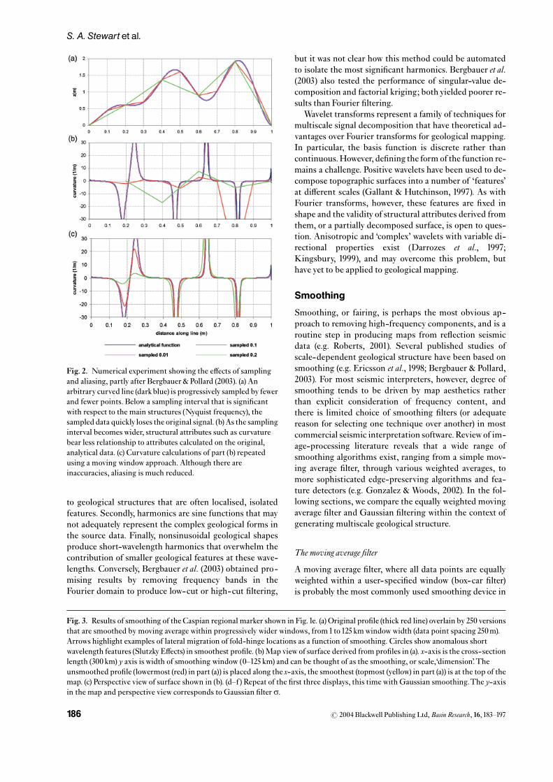
Bergbauer & Pollard (2003) reject decimation as a me-chanism for removing high frequencies, on the basis ofaliasing. An experiment published by Bergbauer & Pollard(2003, their Fig.11) is reproduced here (Fig. 2a, b), demon-strating how progressive undersampling of an arbitraryanalytical function produces distortion (i.e. aliasing) of theoriginal form. This distortion is initially manifest aschanges in the position and shape of fold hinges, until ¢ -nally the original form becomes unrecognisable (Fig. 2a).The onset of aliasing depicted in Fig. 2a is re£ected in at-tributes such as curvature (Fig. 2b).

An alternative approach to decimation involves a ‘mov-ing window’ where the data points are sampled for attri-bute calculation at some desired sampling interval.Unlike decimation as described above, this process is re-peated at each data pointwithin the initial high-resolution

data set, so the derived data has the same number of datapoints as the original data set (minus some data pointsaround themargins of the surfacewhere the samplingwin-dow half-width exceeds the distance to the data set edge).The moving-window approach is less prone to aliasing as-sociated with the sampling frequency because the sam-pling is repeated at every grid node in the initial data set(Stewart & Podolski, 1998; Bel¢eld, 2000; Stewart &Wynn,2000). Figure 2c illustrates the results of curvature mea-surements at the same resampling intervals used in Fig.2b, and demonstrates that the aliasing problems such asfold-hinge misposition are much reduced.

Decomposition

Fourier transforms are widely used for decomposing con-tinuous signals into their component frequencies, andhave been applied to geological fold shape (Stabler, 1968;Ramsay & Huber, 1987; Stowe, 1988), geomorphologicalsurfaces (Pike & Rozema, 1975) and bedding surfacesmapped on 3D seismic in sedimentary basins (Bergbaueret al., 2003). Gallant & Hutchinson (1997) critically dis-cussed applying Fourier spectral analysis to regional geo-logical surfaces.They pointed out that Fourier harmonicsare continuous within an area of interest; consequently,their properties are independent of location, in contrast

Fig.1. Re£ection seismic examples (2D pro¢les) of scale-dependent structure from two sedimentary basins. (a, b) from the centralNorth Sea show a mixture of geological structure and seismic noise at sub-kilometre scale (a), and structures up to basin curvature at ascale of hundreds of kilometres (b). (cê) show the relatively simple, kilometre-scale fold train of the south Caspian Sea. Additionalstructures are seen within the folds (c) and at basin scale (e).

r 2004 Blackwell Publishing Ltd,Basin Research, 16, 183^197 185

Multiscale geological structure

to geological structures that are often localised, isolatedfeatures. Secondly, harmonics are sine functions that maynot adequately represent the complex geological forms inthe source data. Finally, nonsinusoidal geological shapesproduce short-wavelength harmonics that overwhelm thecontribution of smaller geological features at these wave-lengths. Conversely, Bergbauer et al. (2003) obtained pro-mising results by removing frequency bands in theFourier domain to produce low-cut or high-cut ¢ltering,

but it was not clear how this method could be automatedto isolate the most signi¢cant harmonics. Bergbauer et al.(2003) also tested the performance of singular-value de-composition and factorial kriging; both yielded poorer re-sults than Fourier ¢ltering.

Wavelet transforms represent a family of techniques formultiscale signal decomposition that have theoretical ad-vantages over Fourier transforms for geological mapping.In particular, the basis function is discrete rather thancontinuous.However, de¢ning the form of the function re-mains a challenge. Positive wavelets have been used to de-compose topographic surfaces into a number of ‘features’at di¡erent scales (Gallant & Hutchinson, 1997). As withFourier transforms, however, these features are ¢xed inshape and the validity of structural attributes derived fromthem, or a partially decomposed surface, is open to ques-tion. Anisotropic and ‘complex’ wavelets with variable di-rectional properties exist (Darrozes et al., 1997;Kingsbury, 1999), and may overcome this problem, buthave yet to be applied to geological mapping.

Smoothing

Smoothing, or fairing, is perhaps the most obvious ap-proach to removing high-frequency components, and is aroutine step in producing maps from re£ection seismicdata (e.g. Roberts, 2001). Several published studies ofscale-dependent geological structure have been based onsmoothing (e.g. Ericsson et al., 1998; Bergbauer & Pollard,2003). For most seismic interpreters, however, degree ofsmoothing tends to be driven by map aesthetics ratherthan explicit consideration of frequency content, andthere is limited choice of smoothing ¢lters (or adequatereason for selecting one technique over another) in mostcommercial seismic interpretation software. Review of im-age-processing literature reveals that a wide range ofsmoothing algorithms exist, ranging from a simple mov-ing average ¢lter, through various weighted averages, tomore sophisticated edge-preserving algorithms and fea-ture detectors (e.g. Gonzalez & Woods, 2002). In the fol-lowing sections, we compare the equally weighted movingaverage ¢lter and Gaussian ¢ltering within the context ofgenerating multiscale geological structure.

The movingaverage ¢lter

A moving average ¢lter, where all data points are equallyweighted within a user-speci¢ed window (box-car ¢lter)is probably the most commonly used smoothing device in

Fig. 2. Numerical experiment showing the e¡ects of samplingand aliasing, partly after Bergbauer & Pollard (2003). (a) Anarbitrary curved line (darkblue) is progressively sampled by fewerand fewer points. Below a sampling interval that is signi¢cantwith respect to the main structures (Nyquist frequency), thesampled data quickly loses the original signal. (b)As the samplinginterval becomes wider, structural attributes such as curvaturebear less relationship to attributes calculated on the original,analytical data. (c) Curvature calculations of part (b) repeatedusing a moving window approach. Although there areinaccuracies, aliasing is much reduced.

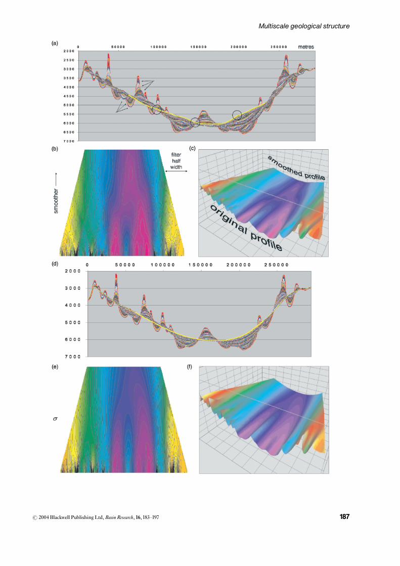
Fig. 3. Results of smoothing of the Caspian regional marker shown in Fig.1e. (a) Original pro¢le (thick red line) overlain by 250 versionsthat are smoothed by moving average within progressively wider windows, from1to125 kmwindow width (data point spacing 250m).Arrows highlight examples of lateral migration of fold-hinge locations as a function of smoothing. Circles show anomalous shortwavelength features (Slutzky E¡ects) in smoothest pro¢le. (b)Map view of surface derived from pro¢les in (a). x-axis is the cross-sectionlength (300 km) y axis is width of smoothing window (0^125 km) and can be thought of as the smoothing, or scale,‘dimension’.Theunsmoothed pro¢le (lowermost (red) in part (a)) is placed along thex-axis, the smoothest (topmost (yellow) in part (a)) is at the top of themap. (c) Perspective view of surface shown in (b). (d^f) Repeat of the ¢rst three displays, this time withGaussian smoothing.The y-axisin the map and perspective view corresponds to Gaussian ¢lters.





geological mapping (e.g. Bergbauer &Pollard, 2003). It canbe shown, however, that equal weighting is less e¡ectivethan a weighted mean for the purposes of eliciting scale-dependent structure. Figure 3 shows the e¡ect of applyingmoving average smoothing to the folded regional markershown inFig.1e. In this experiment, the original 2Dpro¢lewas smoothed by a moving average ¢lter with 250 di¡erentkernel sizes (kernel is an arrangement of numbers thatconstitute a ¢lter). The narrowest ¢lter was three datapoints wide (a 1� 3 kernel resampling a 500-m window)and the resulting curve is plotted immediately on top ofthe original pro¢le in Fig. 3a.This result is then superim-posed by the results from the other 249 kernel sizes, culmi-nating in the widest (1 � 501 kernel resampling a 125-kmwindow) and represents the topmost pro¢le plotted (inbold yellow) on Fig. 3a. The consecutively smoother ver-sions of the original surface can also be used to constructa 3D surface to help visualise the scale dimension, or scale-space (Fig. 3b, c).The lateral migration (mispositioning) offold hinges noted in the resampling example (Fig. 2a) isseen once again with progressive moving average smooth-ing (Fig. 3a^c).The most heavily smoothed pro¢le (yellowin Fig. 3a) shows that relatively short wavelength structurehas persisted, or been created, in spite of the aggressive le-vel of smoothing.These phenomena are known as Slutzkye¡ects after an economist who showed that a moving aver-age might generate an irregular oscillation even if none ex-ists in the original data (Slutzky, 1937).

Gaussian ¢ltering

An alternative to the arithmetic mean is some form ofweighted average, either linear or more complex. In a dis-cussion of scale dependence in topography,Wood (1996)suggested that distance-dependent weighting should beuser-de¢ned (but criteriawere not speci¢ed). An approachcommonly employed in image and signal processing isweighting according to a Gaussian function (Eqn. (1) de-¢nes a one-dimensional Gaussian ¢lter).

GðxÞ ¼ 1

sffiffiffiffiffi2p

p e�x2=2s2 ð1Þ

where x is distance from the median point of the ¢lter ands is the standard deviation that de¢nes the shape (width) ofthe weighting pro¢le. Widespread usage of Gaussiansmoothing re£ects a number of advantageous properties,including, spatial shift invariance (i.e. no preferred loca-tion of ¢lter), thus all locations are measured in the samefashion. Isotropy (i.e. no preferred orientation of ¢lter),and no new structures are created in the transition from¢ne to coarse scale. Babaud et al. (1986),Weickert (1997),Lindeberg (1999) andHay etal. (2002) discussGaussian ¢l-tering in more detail and conclude that this family ofsmoothing operators is a good choice for multiscale analy-sis ^ especially without a priori information. Figure 3d^frepeat the smoothing exercise of Fig. 3a^c, this time con-volving the data representing the regional marker from

Fig. 1e with a Gaussian ¢lter through a range (1^250) ofstandard deviations (s). Figure 3d compared with Fig. 3ashows that the most smoothed (uppermost) pro¢le is freefrom the high-frequency artefacts produced by movingaverage ¢ltering. The relative stability of Gaussiansmoothing is particularly clear in the comparison of mapviews of the surfaces that represent the progressivelysmoothed pro¢le (Fig. 3b, e, c, f). Lateral migration of foldhinges is less pronounced. Given the widespread use ofGaussian smoothing in other disciplines and the relativelygood performance of this approach to smoothing demon-strated here, Gaussian smoothing is adopted here as thecore process for investigating scale-dependent geologicalstructure. Figure 3e can be viewed as a scale-space repre-sentation of the original 2D geological pro¢le (Witkin,1984), and is the basis of the natural scales analysis in thenext section.

2D MULTISCALE GEOLOGICALSTRUCTURE ^ NATURAL SCALES

The 3D surfaces generated by applying aGaussian ¢lter tosmooth a single 2Dpro¢le inFig. 3 show that structure ap-pears to evolve progressively with smoothing, rather thanin a series of abrupt steps, raising the question: with noa priori knowledge of the scale of the geological structuralelements, how canwe identify speci¢c geological frequen-cies in the initial data, given the continuous nature ofscale-space? To address this question, we introduce theconcept of natural scales, which seeks to identify realstructures within a scale-space curve or pro¢le, accordingto some signi¢cance criterion, while excluding the redun-dant information (Bengtsson & Eklundh, 1991; Rosin,1992, 1998).

A technique for determining natural scales

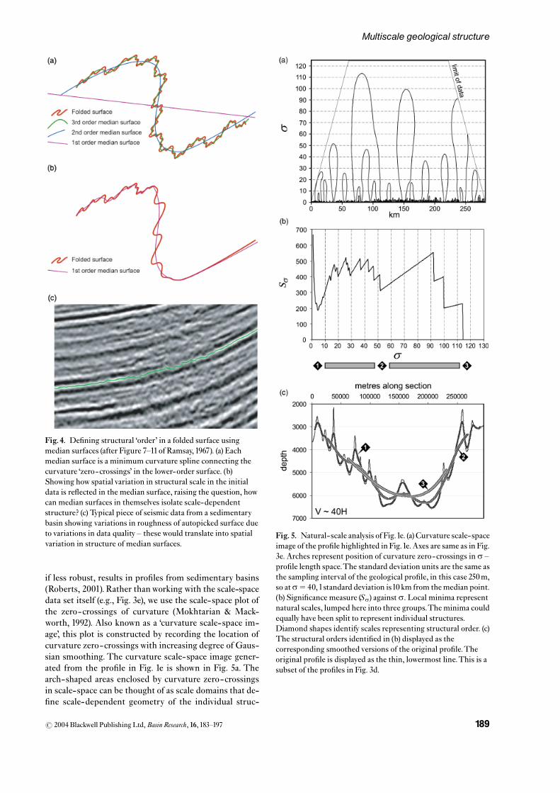
Multiscale analysis requires two main components: thegeneration of a multiscale representation, and a featuredetector. Given a scale-space representation of a pro¢le(Fig. 3e), the problem of detecting natural scales becomesthe task of subdividing scale-space according to structuralsigni¢cance.The technique employed here was describedin a reviewofmethods for calculating natural scales by Ro-sin (1992), which is built on the notion that structures canbe identi¢ed by changes in the sign of curvature. This isconceptually the same condition used by Ramsay (1967,pp. 351^355) to identify hierarchies of median surfaces infold trains (Fig. 4a).The primary weakness of the mediansurface method was that a given order of median surfacecould contain structure at awide variety of scales (Fig. 4b, c),therefore could not isolate scale-speci¢c structure.

Curvature is independent of the overall reference frameof the pro¢le, so delimiting structures by in£ections, or‘zero-crossings’ of curvature, rather than changes fromconcave up to concave down, has the advantage of rotationinvariance. In practice, the second derivative gives similar,



if less robust, results in pro¢les from sedimentary basins(Roberts, 2001). Rather thanworking with the scale-spacedata set itself (e.g., Fig. 3e), we use the scale-space plot ofthe zero-crossings of curvature (Mokhtarian & Mack-worth, 1992). Also known as a ‘curvature scale-space im-age’, this plot is constructed by recording the location ofcurvature zero-crossings with increasing degree of Gaus-sian smoothing. The curvature scale-space image gener-ated from the pro¢le in Fig. 1e is shown in Fig. 5a. Thearch-shaped areas enclosed by curvature zero-crossingsin scale-space can be thought of as scale domains that de-¢ne scale-dependent geometry of the individual struc-

Fig.4. De¢ning structural ‘order’ in a folded surface usingmedian surfaces (after Figure 7^11of Ramsay, 1967). (a) Eachmedian surface is a minimum curvature spline connecting thecurvature ‘zero-crossings’ in the lower-order surface. (b)Showing how spatial variation in structural scale in the initialdata is re£ected in the median surface, raising the question, howcan median surfaces in themselves isolate scale-dependentstructure? (c) Typical piece of seismic data from a sedimentarybasin showing variations in roughness of autopicked surface dueto variations in data quality ^ these would translate into spatialvariation in structure of median surfaces.

Fig. 5. Natural-scale analysis ofFig.1e. (a)Curvature scale-spaceimage of the pro¢le highlighted inFig.1e. Axes are same as in Fig.3e. Arches represent position of curvature zero-crossings ins ^pro¢le length space.The standard deviation units are the same asthe sampling interval of the geological pro¢le, in this case 250m,so ats5 40,1standard deviation is10 km from the median point.(b) Signi¢cance measure (Ss) againsts. Local minima representnatural scales, lumped here into three groups.The minima couldequally have been split to represent individual structures.Diamond shapes identify scales representing structural order. (c)The structural orders identi¢ed in (b) displayed as thecorresponding smoothed versions of the original pro¢le.Theoriginal pro¢le is displayed as the thin, lowermost line.This is asubset of the pro¢les in Fig. 3d.



tures they enclose. Archwidth is an indication of structur-al wavelength (distance along the original pro¢le with con-stant curvature sign after a given amount of smoothing),and height is a measure of the scale. Structures do not per-sist (in scale) beyond the crest of their enclosing arches.

The density of zero-crossings as a function of scale isthen used to identify ‘natural scales’. In our de¢nition, nat-ural scales are de¢ned by step changes in the density ofzero-crossings. Visual inspection of Fig. 5a suggests thepresence of several natural scales within the original pro-¢le.The population of the shortest wavelength structuresexists at so5, a loose group of intermediate scale struc-tures are removedwhen15oso50, and three larger struc-tures dominate the interval 90oso110. Beyond s5110only the basin scale structure remains, though it does notappear on Fig. 5a as there are no associated in£ections inthe curve representing the basin (Fig. 3d).We test here anumerical method of identifying these scale-speci¢cgroups, using a signi¢cance measure (Ss). At each scale,Ss is de¢ned as the sum of the number of zero-crossingsof curvature at all points on the curve normalised by theGaussian smoothing scale s (Fig. 5b). Natural scales arede¢ned to be at scales producing local minima of Ss,where individual structures or groups of structures disap-pear (Bengtsson & Eklundh, 1991; Rosin, 1992). Accordingto this criterion, Fig. 5b shows three de¢ned orders ofstructure: the lowest (1) corresponds to the individual foldsseen in Fig. 1e, the highest (3) is the basin scale curvatureseen in Fig. 3e. In Fig. 5c we illustrate the results of apply-ingGaussian ¢ltering to the original pro¢le at these natur-al scales, to reveal optimised orders of structure.

The natural scales shown inFig. 5 are global in the sensethat a smoothing operator of a given scale is convolvedwith all of the original data but the result will only yieldstructure where it exists in the original data, based on spe-ci¢c threshold criteria.Nonetheless, there are several tech-niques available for calculating natural scales locally ratherthan globally (review byRosin, 1998). However, calculationof local natural scales tends to be less stable than the globalmethod, and is not further pursued in this study.

Discussion of natural scales

The results in Fig. 5 show that natural- scale analysis of afold belt with a regional data set can isolate smooth formsof individual fold structures, and at the largest scale, detectbasinal curvature that is di⁄cult to measure in the initialdata.The ¢rst natural scale e¡ectively removes the highestfrequency noise in the data/interpretation, but preservesthe wavelength and amplitude characteristics of the majorfold structures.This low-order natural scale could be usedin curvature analysis to determine strain distribution andrelated reservoir parameters (e.g. Ericsson et al., 1998; Ro-berts, 2001; Hart et al., 2002). The higher-order, larger-scale structures are not obvious within spatially restrictedsubsets of data, but could contribute to the ¢nite strainwithin the deformed layers and could also be the subjectof curvature analysis to factorise scale-speci¢c structure

from the total strain at outcrop or well scale (Stewart &Wynn, 2000). An alternative approach would be to use ahigh-order natural scale as a structural restoration tem-plate to remove basin curvature (for example) before strainanalysis.The di¡erence between the ¢rst natural scale and



the original data, or between low-order natural scales isthe equivalent of applying a low-cut ¢lter and can reveal,for example, sedimentary features by removing local foldstructures (e.g. Fig. 8 of Carter, 2003).

Gaussian ¢ltering reduces the area enclosed by thecurve or surface (e.g. Lowe, 1989). This ‘shrinkage’ a¡ectsclosed curves (e.g. diapirs) more severely than open ones(e.g. regional bedding planes). It can be measured and cor-rected by various methods, such as normalising the inte-grals of the original and smoothed curves (Desbrun et al.,1999).TheFig. 3d examples show a maximum shrinkage of3.5% (ats5125).The examples in Fig. 6 include a shrink-age correction method described by Lowe (1989).

Several di¡erent geological data sets were used to testthe method further. The results are illustrated in Fig. 6.Figure 6a represents a stratigraphic marker overlying a saltdiapir in the central North Sea. The ¢rst natural scale isdi⁄cult to distinguish from the initial data and retainsrugosity due to local degradation in seismic data quality.The second natural scale removes this rugosity but pre-serves the overall form of the drape fold, and some adja-cent deepwater channels. The third scale emphasises thewavelength of the large features in the surface but doesnot represent the shape of these structures accurately. Fig-ure 6b is a section through two deepwater channel cuts.The natural scales yield the same information as discussedfor Fig. 6a, but it is now clearer that the third natural scaleis a poor representation of the structural form even thoughthe wavelength is accurately measured. It is also evidentthat the structural amplitude is suppressed in spite of hav-ing been corrected for shrinkage.The examples so far havebeen free from abrupt changes in dip.

Faulted surfaces, on the other hand, challenge all meth-ods of analysing scale-dependent structure. The mainproblems are the sharp edges at fault cuto¡s and the spa-tial gaps in structure between the fault cuto¡s. Figure 6cshows a faulted surface in which interpretation of the re-gional marker is connected by interpretation along thefault planes, giving a combination of sharp edges, faultplanes and unfaulted strata within the fault blocks. Thenatural-scale surfaces treat the whole data set as a contin-uous curve and do not distinguish between the fault planesand unfaulted strata. Solving this issue is beyond the scopeof this paper, though there are some obvious geometricalpossibilities such as restricting natural- scale analysis tostrata within major fault blocks, or doing natural- scaleanalysis on a surface with the major faults restored. Figure6d shows natural- scale analysis of a topographic pro¢le

from a present day mountain range. In this case, naturalscales isolate the position and areal extent of the principaltopographic features.

In each of the cases shown in Fig. 6, as in Fig. 5, manualinputwas required at the stage ofdecidingwhether to‘lumpor split’ the natural scales detected by Ss minima. So thetechnique involves an element of interpretation and is bestdescribed as ‘semi-automatic’. Nonetheless, it represents astep forward in the structural analysis of seismic interpre-tation by objectively identifying scales of interest that cango forward into further attribute analysis. Although theanalysis has been on 2D sections rather than 3D surfacesso far, 2D analysis can represent a rapid, automated guideto determine the degree of smoothing to be applied to largesurface data sets prior to further analysis (e.g. curvaturemeasurement).The next section of this paper describes ap-plication of a similar technique to 3D surfaces.

3D MULTISCALE GEOLOGICALSTRUCTURE ^ SCALE-SPACETOPOLOGY

Multiscale analysis of a 3D surface is done in two stages ^similar to the approach to analysing 2D pro¢les ^ gene-ration of scale-space, followed by feature detection. Sev-eral methods are available along these lines (Hay et al.,2003). We generate ‘linear scale-space’ (Lindeberg, 1994;Hay et al., 2002) to provide a multiscale representation ofa geological surface mapped on 3D re£ection seismic data(i.e. a gridded surface, or digital elevation model), and em-ploy ‘blob-feature detection’ (Hay et al., 2002) for automa-tically de¢ning dominant multiscale components fromthis representation.

Linear scale space

Scale-space is an uncommitted framework for early visualoperations that was developed by the computer visioncommunity to automatically analyse real-world structuresat multiple scales ^ speci¢cally, when there is no apriori in-formation about these structures, or the appropriatescale(s) for their analysis (Lindeberg, 1994).‘Uncommittedframework’ refers to observations made by a front-end vi-sion system (i.e. an initial-stage measuring device) such asthe retina, a camera or a re£ection seismic survey that in-volves no knowledge, and no preference for anything.When no scale information is known about a map or visualscene, the only reasonable approach for an uncommittedvision system is to represent the input data at (all) multiplescales. The example chosen here to test this method in ageological context is a patch of 3D seismic interpretationfrom a surface overlying a salt diapir in the Central NorthSea, that is known to contain a variety of types of geologi-cal and artefact structure at various scales (Fig. 7a, b).

In practice, surface elevation is treated as a height attri-bute, enabling the surface to be converted to a greyscaleimage, or map. Gaussian ¢lters are applied to this initial

Fig. 6. Natural scales in various cross- sections. Each exampleshows the initial pro¢le as a thin black line overlain by the ¢rstthree natural scales. Axis labels in metres, all have signi¢cantvertical exaggeration (labelled). (a) Drape fold overlying NorthSea diapir. (b) Deep water channel cuts in North SeaMiocenesurface. (c) Faulted intra-Permian surface, southern North Sea.Inset shows original interpretation at V5H,with faults marked.(d) Present day topographic pro¢le across the sub-Andeanfoothills, Bolivia.



greyscale image at a range of kernel sizes resulting in ascale-space cube or stack of progressively smoothed imagelayers, where each new image layer represents convolutionat an increased scale (Fig. 7c).This is a process similar tothe smoothing of 2D pro¢les discussed earlier in this pa-

per (Fig. 3cê), though here, we are using the zeroth-orderderivative of a ‘2D’Gaussian function (Eqn. (2)).

Gðx; yÞ ¼ 12ps2 e

� ðx2þy2Þ=2s2ð Þ ð2Þ



As before, the scale of each derived signal is de¢ned by se-lecting a di¡erent standard deviation s for the Gaussianfunction. Each hierarchical layer in a stack represents con-volution at a ¢xed scale, with the smallest scale at the bot-tom, and the largest at the top (Fig. 7c). This scale-spacecube is analogous to the scale-space surface illustrated inFig. 3e.

Blob-feature detection

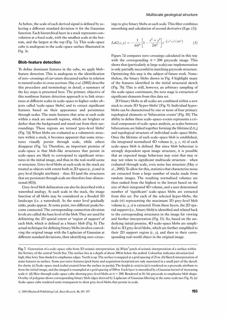
To de¢ne dominant features in the cube, we apply blob-feature detection. This is analogous to the identi¢cationof zero-crossings of curvature discussed earlier in relationto natural scales in cross sections.Hay etal. (2002) describethis procedure and terminology in detail; a summary ofthe key steps is presented here. The primary objective ofthis nonlinear feature detection approach is to link struc-tures at di¡erent scales in scale-space to higher-order ob-jects called ‘scale-space blobs’, and to extract signi¢cantfeatures based on their appearance and persistencethrough scales.The main features that arise at each scalewithin a stack are smooth regions, which are brighter ordarker than the background and stand out from their sur-roundings. These regions are termed ‘grey-level blobs’(Fig. 7d).When blobs are evaluated as a volumetric struc-ture within a stack, it becomes apparent that some struc-tures visually persist through scale, while othersdisappear (Fig. 7e). Therefore, an important premise ofscale-space is that blob-like structures that persist inscale-space are likely to correspond to signi¢cant struc-tures in the initial image, and thus in the real-world sceneor structure. Grey-level blobs at each scale in the stack aretreated as objects with extent both in 2D space (x, y) and ingrey level (height attribute) ^ thus 3D (and the structuresthat are persistent through scale are therefore four-dimen-sional (4D)).

Grey-level blob delineation can also be describedwith awatershed analogy. At each scale in the stack, the imagefunction of all blobs may be considered as a £ooded 3Dlandscape (i.e. a watershed). As the water level graduallysinks, peaks appear. At some point, two di¡erent peaks be-come connected.The corresponding connection elevationlevels are called the base level of the blob.They are used fordelimiting the 2D spatial extent or ‘region of support’ ofeach blob, which is de¢ned as a binary blob (Fig. 8). Theactual technique for de¢ning binary blobs involves convol-ving the original image with the Laplacian of Gaussian atdi¡erent standard deviations, then identifying zero-cross-

ings to give binary blobs at each scale.This ¢lter combinessmoothing and calculation of second derivative (Eqn. (3)).

LoGðx; yÞ ¼ � 1ps4 1� x2 þ y2

2s2

� �e� ðx2þy2Þ=2s2ð Þ ð3Þ

Figure 7d compares zero-crossings calculated in this waywith the corresponding s5 200 greyscale image. Thisshows that (particularly at large scale) our implementationis only partially successful in matching greyscale structure.Optimizing this step is the subject of future work. None-theless, the binary blobs shown in Fig. 8 highlight manyof the features identi¢ed in the initial structural sketch(Fig. 7b). This is still, however, an arbitrary sampling ofthe scale-space continuum; the next stage is extraction ofsigni¢cant elements from this data set.

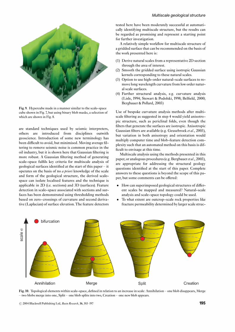
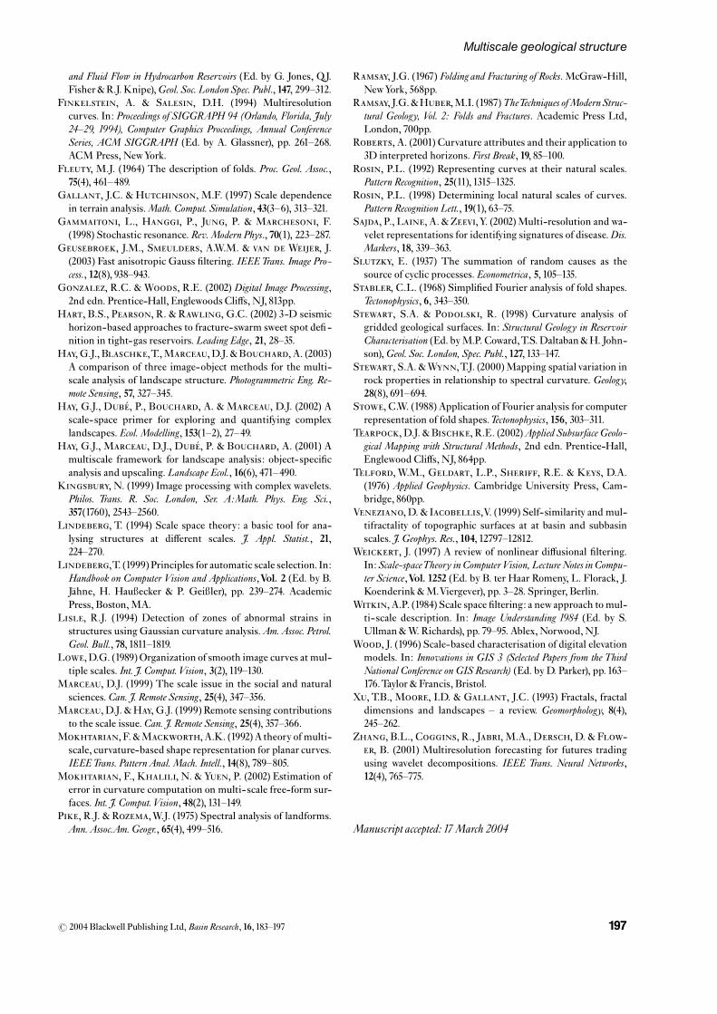
2D binary blobs at all scales are combinedwithin a newstack to create 3D ‘hyper-blobs’ (Fig. 9). Individual hyper-blobs can be characterised by one or more of four primarytopological elements or ‘bifurcation events’ (Fig. 10).Theability to de¢ne these scale-space-events represents a cri-tical component of scale-space analysis, as scales betweenbifurcations are linked together forming the lifetime (Lsn)and topological structure of individual scale-space blobs.Once the lifetime of each scale-space blob is established,the integrated normalised 4D volume (x, y, z, s) of eachscale-space blob is de¢ned. But since blob behaviour isstrongly dependent upon image structure, it is possiblethat an expected image behaviour may exist that may ormay not relate to signi¢cant multiscale structure ^ whenevaluated through scale, even noise has structure (Hay etal., 2002).To allow for this, statistics that characterise noiseare extracted from a large number of stacks made fromrandom images. The resulting normalised volumes arethen ranked from the highest to the lowest based on thesize of their integrated 4D volume, and a user determinednumber of ‘signi¢cant’ scale-space blobs are extractedfrom this set. For each of the selected hyper-blobs, thescale (s) representing the maximum 3D grey-level blobvolume (x, y, z) is extracted. From these layers, the 2D spa-tial support (i.e., binary blob) is identi¢ed and related backto the corresponding structures in the image for viewingand further interpretation (Fig. 11). So, based on the un-derlying initial premise, 4D scale-space blobs are simpli-¢ed to 3D grey-level blobs, which are further simpli¢ed totheir 2D support region (x, y), and then to their corre-sponding real-world object in the original image.

Fig.7. Generation of a scale-space cube from 3D seismic interpretation. (a) 30 km2 patch of seismic interpretation of a surface withintheTertiary of the central North Sea.The surface lies at a depth of about 300m below the seabed. Colourbar indicates elevation (redhigh, blue low). Sun shaded to emphasise edges.North is up.The surface is mapped at a grid spacing of 25m. (b) Sketch interpretation ofmain features in surface. Some pervasive features (pick busts and acquisition footprint) are only annotated in a small part of the sketchfor clarity. (c) Scale- space stack (cube) created from the surface in part(a).The height (z-axis) in (a) is rendered as a greyscale attribute toform the initial image, and the imaged is resampled at a grid spacing of100m. Each layer is smoothed by aGaussian kernel of increasingscales. (d) Slice through scale- space cube showing grey-level blobs ats5 200. Rendered in16-bit greyscale to emphasise blob shape.Overlay of polygons shows corresponding binary blob edges derived by Laplacian of Gaussian ¢ltering at the same scale (see Fig. 8). (e)Scale-space cube rendered semi-transparent to show grey-level blobs that persist in scale.



Discussion of blob-feature detection

This analysis yielded 4635 hyper-blobs, each representedbya 2D support region polygon.This represents automaticselection of 2D blobs corresponding to features that werearbitrarily intersected in the scale slices shown in Fig. 8.Visual appraisal of this large number of features is a sub-stantial task in itself. Figure11a shows 200 of the most sig-ni¢cant blobs, rendered as un¢lled 2D support regionpolygons.Even this small proportion (4%of the total iden-ti¢ed) is di⁄cult to make sense of in a conventional mapdisplay. For clarity, in this short discussion the number isfurther reduced in Fig. 11b. Strengths and weaknesses ofthis approach are clear.The method has identi¢ed small-scale features (pick busts), and large-scale features (saltdome and erosive channels). On the other hand, narrowlinear features such as the radial faults and the seismic ac-quisition footprint have not been identi¢ed as discrete ele-

ments. Furthermore, some large features are only partiallyidenti¢ed, for example the channel in the north of the area.There are also numerous circular features of approxi-mately 500-m diameter that are not obvious in the originaldata set (Fig. 7a) ^ it is unclear if these are artifacts of theprocess or if they are a subtle geological phenomenon suchas incipient polygonal faults. It is, however, encouragingthat structures over a range of scales have been identi¢edby this automatic procedure, but further work is evidentlyrequired to simplify the output of the feature detector.

SUMMARY

The density and extent of data acquired in seismic re£ec-tion surveys allows multiscale structural analysis. A num-ber of possible methods for deriving scale-space anddetecting structures within it have been reviewed ^ some

Fig. 8. Binary blobs derived by Laplacian of Gaussian ¢ltering of the intial greyscale image at a range of scales, comparedwith thesource seismic interpretation.The binary blobs highlight di¡erent features at di¡erent scales.



are standard techniques used by seismic interpreters,others are introduced from disciplines outwithgeoscience. Introduction of some new terminology hasbeen di⁄cult to avoid, but minimised.Moving average ¢l-tering to remove seismic noise is common practice in theoil industry, but it is shown here that Gaussian ¢ltering ismore robust. A Gaussian ¢ltering method of generatingscale-space ful¢ls key criteria for multiscale analysis ofgeological surfaces identi¢ed at the start of this paper ^ itoperates on the basis of no a priori knowledge of the scaleand form of the geological structure, the derived scale-space can isolate localised features and the technique isapplicable in 2D (i.e. sections) and 3D (surfaces). Featuredetection in scale-space associated with sections and sur-faces has been demonstrated using thresholding methodsbased on zero-crossings of curvature and second deriva-tive (Laplacian) of surface elevation.The feature detectors

tested here have been moderately successful at automati-cally identifying multiscale structure, but the results canbe regarded as promising and represent a starting pointfor further investigation.

A relatively simple work£ow for multiscale structure ofa gridded surface that can be recommended on the basis ofthe work presented here is:

(1) Derive natural scales from a representative 2D sectionthrough the area of interest.

(2) Smooth the gridded surface using isotropic Gaussiankernels corresponding to these natural scales.

(3) Option to use high-order natural- scale surfaces to re-move long wavelength curvature from low order natur-al scale surfaces.

(4) Further structural analysis, e.g. curvature analysis(Lisle, 1994; Stewart & Podolski, 1998; Bel¢eld, 2000;Bergbauer & Pollard, 2003)

Use of bespoke curvature analysis methods after multi-scale ¢ltering as suggested in step 4 would yield anisotro-pic structure, such as periclinal folds, even though the¢lters that generate the surfaces are isotropic. AnisotropicGaussian ¢lters are available (e.g. Geusebroek et al., 2003),but variation in both anisotropy and orientation wouldmultiply computer time and blob-feature detection com-plexity such that an automated method on this basis is dif-¢cult to envisage at this time.

Multiscale analysis using the methods presented in thispaper, or analogous procedures (e.g. Bergbauer etal., 2003),are appropriate for addressing the structural geologyquestions identi¢ed at the start of this paper. Completeanswers to these questions is beyond the scope of this pa-per, but some comments can be o¡ered:

� How can superimposed geological structures of di¡er-ent scales be mapped and measured? Natural- scaleanalysis and scale-space topology could be used.

� To what extent are outcrop-scale rock properties likefracture permeability determined by larger scale struc-

Fig.9. Hypercube made in a manner similar to the scale- spacecube shown in Fig. 7, but using binary blob masks, a selection ofwhich are shown in Fig. 8.

Fig.10. Topological elements within scale-space, de¢ned in relation to an increase in scale: Annihilation ^ one blob disappears,Merge^ two blobs merge into one, Split ^ one blob splits into two, Creation ^ one new blob appears.



tures that may be unseen at outcrop or in thewellbore?Structures or structural domains identi¢ed in scale-space are candidates for controlling widespread frac-ture sets.

� Should fold-classi¢cation schemes be quali¢ed withscale-dependent terms? The examples presented inthis paper strongly indicate that whether a fold is per-ceived or not depends entirely on the scale of observa-tion, so a measure of fold scale should alwaysaccompany classi¢cation that is otherwise based onfold style or geometry. Scale-space analysis could un-derpin a novel, automated method of fold mappingand classi¢cation.

� Are interference and parasitic fold patterns end-mem-bers of a continuum? This could be the case in geo-metric, if not genetic, terms.

Possible applications of these methods in a hydrocarbonproduction context are indicated above; speci¢c examplesinclude automated removal of data noise from seismic in-terpretation and mapping of tectonically in£uenced reser-voir quality domains.

ACKNOWLEDGMENTS

The opinions expressed here are solely those of theauthors and not necessarily those of BP orTRACS Inter-national. The paper bene¢ted from reviews by R. Lisleand S. Bergbauer. H.Macintyre and R. Hardy are thankedfor bringing key work to the authors’attention.

REFERENCES

Babaud, J.,Witkin,A.P.,Baudin,M.&Duda,R.O. (1986) Un-iqueness of theGaussian kernel for scale-space ¢ltering. IEEETrans. Pattern Anal.Mach. Intell., 8(1), 26^33.

Belfield, W.C. (1998) Incorporating spatial distribution intostochastic modelling of fractures: multifractals and Le¤ vy-stable statistics. J. Struct. Geol., 20, 473^486.

Belfield,W.C. (2000) Predicting natural fracture distributionin reservoirs from 3D seismic estimates of structural curva-ture. SPE E-Library Paper No. 60298.

Bengtsson,A.&Eklundh, J.O. (1991)Shape representation bymultiscale contour approximation. IEEE Trans. Pattern Anal.Mach. Intell., 13(1), 85^93.

Bergbauer, S.,Mukerji,T. & Hennings, P. (2003) Improvingcurvature analyses of deformed horizons using scale-depen-dent ¢ltering techniques.AmericanAssociation of PetroleumGeol-ogists Bulletin, 87(8), 1255^1272.

Bergbauer,S.&Pollard,D.D. (2003)How to calculate normalcurvatures of sampled geological surfaces. J. Struct. Geol., 25,277^289.

Bonnet,E.,Bour,O.,Odling,N.E.,Davy,P.,Main, I.,Cow-ie,P.&Bekowitz,B. (2001)Scaling of fracture systems in geo-logical media.Rev. Geophys., 39(3), 347^383.

Carter,D.C. (2003) 3-D seismic geomorphology: insights into£uvial reservoir performance,Widuri Field, Java Sea. Am. As-soc. Petrol. Geol. Bull., 87, 909^934.

Cowie, P.A., Sornette,D. & Vanneste, C. (1995) Multifractalscaling properties of a growing fault population. Geophys. J.Int., 122, 457^469.

Darrozes, J., Gaillot, P., Saint-Blanquat,M. & Bouchez,J.L. (1997) Software for multiscale image analysis: the nor-malized optimized anisotropic wavelet coe⁄cient method.Comput. Geosci., 23(8), 889^895.

Desbrun, M., Meyer, M., Schr˛der, P. & Barr, A.H. (1999)Implicit fairing of irregular meshes using di¡usion and curva-ture £ow. Proceedings SIGGRAPH ’99, Computer GraphicsProceedings, Annual Conference Series, pp. 317^324. ACMPress, NewYork.

Ericsson, J.B., McKean, H.C. & Hooper, R.J. (1998) Faciesand curvature controlled 3D fracture models in a cretaceouscarbonate reservoir, Arabian Gulf. In: Faulting, Fault Sealing

Fig.11. Selection of 2D polygons or support regions,corresponding to 4D hyper-blobs identi¢ed as beingsigni¢cantly di¡erent from noise. (a) 200 of the most signi¢cantsupport regions overlaid on thes5 200derivation of the originalimage. (b) User-de¢ned ‘top thirty’ support regions (large onesshaded darker) comparedwith interpretation of the initial image.



and Fluid Flow in Hydrocarbon Reservoirs (Ed. by G. Jones, Q.J.Fisher &R.J. Knipe),Geol. Soc. London Spec. Publ., 147, 299^312.

Finkelstein, A. & Salesin, D.H. (1994) Multiresolutioncurves. In: Proceedings of SIGGRAPH 94 (Orlando, Florida, July24^29, 1994), Computer Graphics Proceedings, Annual ConferenceSeries, ACM SIGGRAPH (Ed. by A. Glassner), pp. 261^268.ACM Press, NewYork.

Fleuty, M.J. (1964) The description of folds. Proc. Geol. Assoc.,75(4), 461^489.

Gallant, J.C. & Hutchinson, M.F. (1997) Scale dependencein terrain analysis.Math. Comput. Simulation, 43(3^6), 313^321.

Gammaitoni, L., Hanggi, P., Jung, P. & Marchesoni, F.(1998) Stochastic resonance.Rev.Modern Phys., 70(1), 223^287.

Geusebroek, J.M., Smeulders, A.W.M. & van de Weijer, J.(2003) Fast anisotropic Gauss ¢ltering. IEEETrans. Image Pro-cess., 12(8), 938^943.

Gonzalez, R.C. & Woods, R.E. (2002) Digital Image Processing,2nd edn. Prentice-Hall, Englewoods Cli¡s, NJ, 813pp.

Hart, B.S., Pearson, R. & Rawling,G.C. (2002) 3-D seismichorizon-based approaches to fracture-swarm sweet spot de¢ -nition in tight-gas reservoirs. Leading Edge, 21, 28^35.

Hay,G.J.,Blaschke,T.,Marceau,D.J.&Bouchard,A. (2003)A comparison of three image-object methods for the multi-scale analysis of landscape structure. Photogrammetric Eng. Re-mote Sensing, 57, 327^345.

Hay, G.J., Dube¤ , P., Bouchard, A. & Marceau, D.J. (2002) Ascale- space primer for exploring and quantifying complexlandscapes. Ecol. Modelling, 153(1^2), 27^49.

Hay, G.J., Marceau, D.J., Dube¤ , P. & Bouchard, A. (2001) Amultiscale framework for landscape analysis: object-speci¢canalysis and upscaling. Landscape Ecol., 16(6), 471^490.

Kingsbury,N. (1999) Image processing with complex wavelets.Philos. Trans. R. Soc. London, Ser. A:Math. Phys. Eng. Sci.,357(1760), 2543^2560.

Lindeberg,T. (1994) Scale space theory: a basic tool for ana-lysing structures at di¡erent scales. J. Appl. Statist., 21,224^270.

Lindeberg,T. (1999)Principles for automatic scale selection. In:Handbook on Computer Vision and Applications,Vol. 2 (Ed. by B.J�hne, H. Hau�ecker & P. Gei�ler), pp. 239^274. AcademicPress, Boston,MA.

Lisle, R.J. (1994) Detection of zones of abnormal strains instructures using Gaussian curvature analysis.Am. Assoc. Petrol.Geol. Bull., 78, 1811^1819.

Lowe,D.G. (1989)Organization of smooth image curves at mul-tiple scales. Int. J. Comput.Vision, 3(2), 119^130.

Marceau, D.J. (1999) The scale issue in the social and naturalsciences.Can. J. Remote Sensing, 25(4), 347^356.

Marceau,D.J.&Hay,G.J. (1999) Remote sensing contributionsto the scale issue.Can. J. Remote Sensing, 25(4), 357^366.

Mokhtarian,F.&Mackworth,A.K. (1992)A theory of multi-scale, curvature-based shape representation for planar curves.IEEETrans. Pattern Anal.Mach. Intell., 14(8), 789^805.

Mokhtarian, F.,Khalili,N. & Yuen, P. (2002) Estimation oferror in curvature computation on multiscale free-form sur-faces. Int. J. Comput.Vision, 48(2), 131^149.

Pike, R.J. & Rozema,W.J. (1975) Spectral analysis of landforms.Ann. Assoc.Am. Geogr., 65(4), 499^516.

Ramsay, J.G. (1967) Foldingand Fracturing of Rocks. McGraw-Hill,NewYork, 568pp.

Ramsay, J.G.&Huber,M.I. (1987)TheTechniques ofModernStruc-tural Geology, Vol. 2: Folds and Fractures. Academic Press Ltd,London, 700pp.

Roberts,A. (2001) Curvature attributes and their application to3D interpreted horizons. First Break, 19, 85^100.

Rosin, P.L. (1992) Representing curves at their natural scales.Pattern Recognition, 25(11), 1315^1325.

Rosin, P.L. (1998) Determining local natural scales of curves.Pattern Recognition Lett., 19(1), 63^75.

Sajda, P.,Laine,A.&Zeevi,Y. (2002)Multi-resolution and wa-velet representations for identifying signatures of disease.Dis.Markers, 18, 339^363.

Slutzky, E. (1937) The summation of random causes as thesource of cyclic processes. Econometrica, 5, 105^135.

Stabler, C.L. (1968) Simpli¢ed Fourier analysis of fold shapes.Tectonophysics, 6, 343^350.

Stewart, S.A. & Podolski, R. (1998) Curvature analysis ofgridded geological surfaces. In: Structural Geology in ReservoirCharacterisation (Ed. byM.P. Coward,T.S. Daltaban &H. John-son),Geol. Soc. London, Spec. Publ., 127, 133^147.

Stewart, S.A.&Wynn,T.J. (2000)Mapping spatial variation inrock properties in relationship to spectral curvature. Geology,28(8), 691^694.

Stowe,C.W. (1988) Application of Fourier analysis for computerrepresentation of fold shapes.Tectonophysics, 156, 303^311.

Tearpock,D.J.&Bischke,R.E. (2002)Applied Subsurface Geolo-gical Mapping with Structural Methods, 2nd edn. Prentice-Hall,Englewood Cli¡s, NJ, 864pp.

Telford,W.M., Geldart, L.P., Sheriff, R.E. & Keys, D.A.(1976) Applied Geophysics. Cambridge University Press, Cam-bridge, 860pp.

Veneziano,D.& Iacobellis,V. (1999) Self-similarity and mul-tifractality of topographic surfaces at at basin and subbasinscales. J. Geophys. Res., 104, 12797^12812.

Weickert, J. (1997) A review of nonlinear di¡usional ¢ltering.In:Scale-spaceTheory inComputerVision, LectureNotes in Compu-ter Science,Vol. 1252 (Ed. by B. ter Haar Romeny, L. Florack, J.Koenderink &M.Viergever), pp. 3^28. Springer, Berlin.

Witkin,A.P. (1984) Scale space ¢ltering: a new approach to mul-ti-scale description. In: Image Understanding 1984 (Ed. by S.Ullman &W. Richards), pp. 79^95. Ablex, Norwood, NJ.

Wood, J. (1996) Scale-based characterisation of digital elevationmodels. In: Innovations in GIS 3 (Selected Papers from the ThirdNational Conference on GISResearch) (Ed. by D. Parker), pp.163^176.Taylor & Francis, Bristol.

Xu,T.B., Moore, I.D. & Gallant, J.C. (1993) Fractals, fractaldimensions and landscapes ^ a review. Geomorphology, 8(4),245^262.

Zhang, B.L., Coggins, R., Jabri,M.A.,Dersch,D. & Flow-

er, B. (2001) Multiresolution forecasting for futures tradingusing wavelet decompositions. IEEE Trans. Neural Networks,12(4), 765^775.

Manuscript accepted:17March 2004



Date post:	10-Feb-2019
Category:	Documents
Upload:	vantu
View:	213 times
Download:	0 times

BasinResearch...

Documents