Basis-constrained Bayesian Markov-chain Monte Carlo difference inversionfor geoelectrical monitoring of hydrogeologic processes
Erasmus Kofi Oware1, James Irving2, and Thomas Hermans3
ABSTRACT
Bayesian Markov-chain Monte Carlo (McMC) techniques areincreasingly being used in geophysical estimation of hydrogeo-logic processes due to their ability to produce multiple estimatesthat enable comprehensive assessment of uncertainty. StandardMcMC sampling methods can, however, become computationallyintractable for spatially distributed, high-dimensional problems.We have developed a novel basis-constrained Bayesian McMCdifference inversion framework for time-lapse geophysical imag-ing. The strategy parameterizes the Bayesian inversion modelspace in terms of sparse, hydrologic-process-tuned bases, leadingto dimensionality reduction while accounting for the physics of
the target hydrologic process. We evaluate the algorithm oncross-borehole electrical resistivity tomography (ERT) field dataacquired during a heat-tracer experiment. We validate the ERT-es-timated temperatures with direct temperature measurements at twolocations on the ERT plane. We also perform the inversions usingthe conventional smoothness-constrained inversion (SCI). Ourapproach estimates the heat plumes without excessive smoothingin contrast with the SCI thermograms. We capture most of thevalidation temperatures within the 90% confidence interval ofthe mean. Accounting for the physics of the target process allowsthe detection of small temperature changes that are undetectableby the SCI. Performing the inversion in the reduced-dimensionalmodel space results in significant gains in computational cost.
INTRODUCTION
Understanding subsurface processes is critical to the designand efficient management of groundwater and energy resources.Although traditional well-based sampling methods provide valuableinsights into subsurface processes (e.g., LeBlanc et al., 1991), theyare expensive and provide limited spatiotemporal information. Theuse of geophysical methods to investigate spatially continuous hydro-geologic processes is well-documented (e.g., Singha et al., 2015).The inversion of geophysical data is, however, nontrivial due to lim-ited noisy data (ill-posedness) and solution nonuniqueness (Menke,1984). Typically, regularization is required to stabilize the problemand obtain a unique result (Tikhonov and Arsenin, 1977).Traditional regularization constraints impose smoothness and/or
force the solution toward some reference model (Menke, 1984)without accounting for our prior understanding of the physics ofthe target hydrologic process. In solute plume moments’ inferencefrom tomograms, Day-Lewis et al. (2007) show that the choice of
regularization strongly influences the solution, often producingsmoothed-out plumes with mass under-estimation. The coupled(Hinnell et al., 2010) and basis-constrained (Oware et al., 2013)inversion frameworks were developed to address the lack of phys-ics-based prior in the traditional regularization constraints.Although deterministic methods provide simple and computa-
tionally efficient inversion frameworks, stochastic inversion (SI)techniques enable comprehensive interpretation of the estimates(Tarantola, 2005) with the capacity to estimate geologically realisticfeatures (e.g., Oware, 2016). Bayesian Markov-chain Monte Carlo(McMC) is a commonly used SI strategy in hydrogeophysics (e.g.,Irving and Singha, 2010). Standard McMC sampling methods can,however, become computationally expensive when working withspatially distributed (high-dimensional) geophysical parameterfields. In such cases, performing McMC in a reduced-dimensionalspace may help to render the stochastic inverse problem computa-tionally tractable (e.g., Ruggeri et al., 2015). Multivariate statisticaltools for dimensionality reduction (e.g., proper orthogonal decom-
Manuscript received by the Editor 6 September 2018; revised manuscript received 2 December 2018; published ahead of production 19 March 2019; pub-lished online 3 May 2019.
position (POD) or singular value decomposition (SVD), eigenvec-tor, and wavelet transformations) typically find an orthogonal set ofbasis vectors that capture the maximum amount of variability in atraining data set, thereby enabling a sparse representation of thechosen system.Hermans et al. (2016) apply a prediction-focused approach
(PFA) (Satija and Caers, 2015) for direct stochastic prediction ofhydrogeologic parameters without the need for classic inversion.Although PFA circumvents classic inversion of the data, it relieson trained statistical relationship for prediction without the processof actually fitting the data, which limits its ability to reconstructfeatures that are not well-represented in the training data. Further-more, the dimensionality reduction can also be achieved viafrequency-amplitude-based bases and orthogonal moments. Loch-buhler et al. (2014) successfully apply discrete cosine transform(DCT) parameterization of the model space for probabilistic elec-trical resistivity characterization of a lab-scale CO2 injection experi-ment. We contend that, unlike process-tuned, nonparametric bases,the parametric DCT bases are fixed, which will limit their ability toreconstruct complex plume morphologies. In a synthetic example,Laloy et al. (2012) successfully performMcMC in the lower dimen-sional model space related to Legendre moments. In an attempt toproduce realistic plume morphologies with mass conservation, theypredefine mass and morphological features, which imposed hard con-straints that are typically unknown a priori in real-world data. Wepresent a novel basis-constrained Bayesian McMC (BcB-McMC)difference inversion framework to improve monitoring of hydrogeo-logic processes. The method constrains the classical Bayesian inver-sion scheme with hydrologic-process-tuned, nonparametric bases toaccount for the physics of the target process. The key contributions ofthe algorithm are that (1) it allows the incorporation of site-specific,hydrologic-process-tuned nonparametric bases, (2) it parameterizesthe Bayesian inversion problem in the reduced-dimensional space,and (3) it does not require prior specifications of mass and plumegeometric features. It also provides a simple, general frameworkto incorporate bases constructed from different methods for findingorthogonal bases. We illustrate the performance of the algorithmon a field-scale geoelectrical data acquired during a heat-tracerexperiment.In spite of the numerous advantages of SI, most of the SI strategies
in hydrogeophysics have focused on characterization of aquiferheterogeneities (e.g., Linde et al., 2006; Oware, 2016) with limitedtechniques addressing the important subject of subsurface solute-plume characterization. This contribution provides a new perspectiveon SI frameworks for geophysical monitoring of subsurface solute-plumes.
Oware et al. (2013) present the basis-constrained inversion,wherein a vector of the target model σ is expressed as a linear com-bination of its basis vectors B and coefficients c
σ ¼ Bc: (1)
They implement equation 1 in a classical Tikhonov deterministic in-version scheme to infer the optimal set of coefficients from geophysi-cal measurements. Here, we formulate a Bayesian McMC version ofthe basis-constrained inversion as
cpost ¼ cpriorLðσjdobsÞ ¼ cpriorLðB; cjdobsÞ; (2)
where cpost and cprior are the posterior and prior coefficients, respec-tively, and Lð•Þ is the likelihood function, which evaluates the prob-ability of a proposed model given the observed data. We implementequation 2 as a difference inversion framework (LaBrecque andYang, 2001). In addition to its rapid convergence, difference inver-sion is intuitively appealing for monitoring hydrogeologic processesdue to its ability to detect small changes, eliminate systematic errors,and reduce inversion artifacts. Hence, adopting the Bayesian view ofregularization (e.g., MacKay, 1992) for computational stability, wecompute the regularized likelihood as
LðB;c;Wd;βjdobsÞ¼exp
�−1
2ðeT �Wd�eþβcT �Wc�cÞ
�;
(3)
where the data misfit expressed in terms of a difference ise ¼ ½dt − d0� − ½fðBcÞ − fðσ0Þ�, with dt and d0 representing data atthe time-step of interest and background, respectively. The termsfðσ0Þ and fðBcÞ are, respectively, the forward simulations fromthe classical inversion (σ0) of the background data and the proposedmodel. The termWd is the data-weight matrix, β, arbitrarily set to 1e-6 here, is a fitting parameter. The value for β can also be determinedusing the L-curve approach (Hansen and O’Leary, 1993). The termWc denotes the coefficient regularization operator, which containsthe inverse of the fractional contributions of the singular values of thebasis vectors, to impose prior structural constraints on c (e.g., Owareand Moysey, 2014).To summarize the workflow of the BcB-McMC, first, we perform
Monte Carlo simulations of training images (TIs) tuned to the phys-ics of the target hydrologic process to capture, for instance, multiplerates of advection and multiple scales of dispersion and complex-ities in the plume morphologies. We pull all the simulated time lapsehydrologic models together into a single robust library of TIs. Sec-ond, we construct orthogonal bases B from the TIs. Third, to obtainprior distributions of the coefficients cprior, we project the TIs ontoB. Fourth, we propose coefficients from cprior. We accept or rejectthe proposed coefficients based on the classic Metropolis-Hastingsacceptance rule (Metropolis et al., 1953; Hastings, 1970). The pos-terior coefficients are then mapped onto the bases to obtain multiplerealizations of the target.
APPLICATION TO FIELD DATA
Heat-tracer and ERT Experiments
We demonstrate the performance of the algorithm on a field-scaleheat-tracer experiment conducted in an alluvial aquifer and moni-tored with cross-borehole electrical resistivity tomography (XBh-ERT). Details of the heat-tracer and XBh-ERT experimental designsare outlined in Hermans et al. (2015). To summarize, water was con-tinuously pumped to induce groundwater flow toward the pumpingwell. Hot water was then injected continuously in an injection wellfor 24 h. Changes in electrical conductivity were monitored in anXBh-ERT panel perpendicular to the flow direction. Here, we focuson the inversion of the first six time-lapse profiles (e.g., Hermanset al., 2018) acquired at 6, 12, 18, 21.5, 25, and 30 h after the com-mencement of the heat injection. After data filtering (Hermans et al.,2018), all the inversions involved only 410 quadrupoles for each time
A38 Oware et al.
Dow
nloa
ded
05/1
2/19
to 9
8.11
8.16
0.19
9. R
edis
trib
utio
n su
bjec
t to
SEG
lice
nse
or c
opyr
ight
; see
Ter
ms
of U
se a
t http
://lib
rary
.seg
.org
/
step. During the experiments, direct temperatures were monitored intwo piezometers, pz14 and pz15 located along the ERT plane.
Inversion procedure
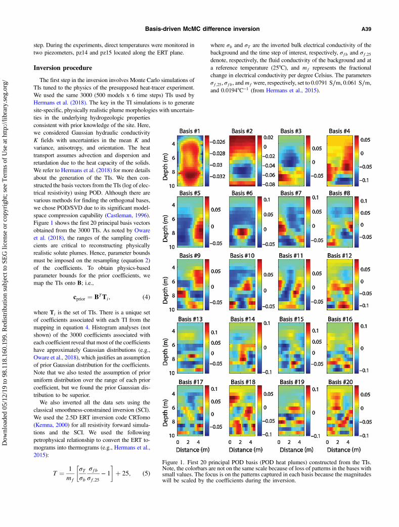
The first step in the inversion involves Monte Carlo simulations ofTIs tuned to the physics of the presupposed heat-tracer experiment.We used the same 3000 (500 models x 6 time steps) TIs used byHermans et al. (2018). The key in the TI simulations is to generatesite-specific, physically realistic plume morphologies with uncertain-ties in the underlying hydrogeologic propertiesconsistent with prior knowledge of the site. Here,we considered Gaussian hydraulic conductivityK fields with uncertainties in the mean K andvariance, anisotropy, and orientation. The heattransport assumes advection and dispersion andretardation due to the heat capacity of the solids.We refer to Hermans et al. (2018) for more detailsabout the generation of the TIs. We then con-structed the basis vectors from the TIs (log of elec-trical resistivity) using POD. Although there arevarious methods for finding the orthogonal bases,we chose POD/SVD due to its significant model-space compression capability (Castleman, 1996).Figure 1 shows the first 20 principal basis vectorsobtained from the 3000 TIs. As noted by Owareet al. (2018), the ranges of the sampling coeffi-cients are critical to reconstructing physicallyrealistic solute plumes. Hence, parameter boundsmust be imposed on the resampling (equation 2)of the coefficients. To obtain physics-basedparameter bounds for the prior coefficients, wemap the TIs onto B; i.e.,
cprior ¼ BTTi; (4)
where Ti is the set of TIs. There is a unique setof coefficients associated with each TI from themapping in equation 4. Histogram analyses (notshown) of the 3000 coefficients associated witheach coefficient reveal that most of the coefficientshave approximately Gaussian distributions (e.g.,Oware et al., 2018), which justifies an assumptionof prior Gaussian distribution for the coefficients.Note that we also tested the assumption of prioruniform distribution over the range of each priorcoefficient, but we found the prior Gaussian dis-tribution to be superior.We also inverted all the data sets using the
classical smoothness-constrained inversion (SCI).We used the 2.5D ERT inversion code CRTomo(Kemna, 2000) for all resistivity forward simula-tions and the SCI. We used the followingpetrophysical relationship to convert the ERT to-mograms into thermograms (e.g., Hermans et al.,2015):
T ¼ 1
mf
�σTσb
σfbσf;25
− 1
�þ 25; (5)
where σb and σT are the inverted bulk electrical conductivity of thebackground and the time step of interest, respectively, σfb and σf;25denote, respectively, the fluid conductivity of the background and ata reference temperature (25°C), and mf represents the fractionalchange in electrical conductivity per degree Celsius. The parametersσf;25, σfb, andmf were, respectively, set to 0.0791 S∕m, 0.061 S∕m,and 0.0194°C−1 (from Hermans et al., 2015).
Figure 1. First 20 principal POD basis (POD heat plumes) constructed from the TIs.Note, the colorbars are not on the same scale because of loss of patterns in the bases withsmall values. The focus is on the patterns captured in each basis because the magnitudeswill be scaled by the coefficients during the inversion.
Basis-driven McMC difference inversion A39
Dow
nloa
ded
05/1
2/19
to 9
8.11
8.16
0.19
9. R
edis
trib
utio
n su
bjec
t to
SEG
lice
nse
or c
opyr
ight
; see
Ter
ms
of U
se a
t http
://lib
rary
.seg
.org
/
RESULTS AND DISCUSSION
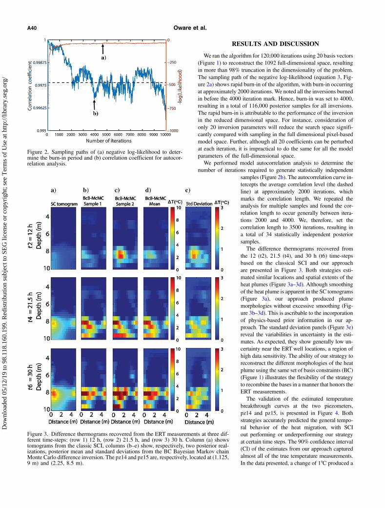
We ran the algorithm for 120,000 iterations using 20 basis vectors(Figure 1) to reconstruct the 1092 full-dimensional space, resultingin more than 98% truncation in the dimensionality of the problem.The sampling path of the negative log-likelihood (equation 3, Fig-ure 2a) shows rapid burn-in of the algorithm, with burn-in occurringat approximately 2000 iterations. We noted all the inversions burnedin before the 4000 iteration mark. Hence, burn-in was set to 4000,resulting in a total of 116,000 posterior samples for all inversions.The rapid burn-in is attributable to the performance of the inversionin the reduced dimensional space. For instance, consideration ofonly 20 inversion parameters will reduce the search space signifi-cantly compared with sampling in the full dimensional pixel-basedmodel space. Further, although all 20 coefficients can be perturbedat each iteration, it is impractical to do the same for all the modelparameters of the full-dimensional space.We performed model autocorrelation analysis to determine the
number of iterations required to generate statistically independentsamples (Figure 2b). The autocorrelation curve in-tercepts the average correlation level (the dashedline) at approximately 2000 iterations, whichmarks the correlation length. We repeated theanalysis for multiple samples and found the cor-relation length to occur generally between itera-tions 2000 and 4000. We, therefore, set thecorrelation length to 3500 iterations, resulting ina total of 34 statistically independent posteriorsamples.The difference thermograms recovered from
the 12 (t2), 21.5 (t4), and 30 h (t6) time-stepsbased on the classical SCI and our approachare presented in Figure 3. Both strategies esti-mated similar locations and spatial extents of theheat plumes (Figure 3a–3d). Although smoothingof the heat plume is apparent in the SC tomograms(Figure 3a), our approach produced plumemorphologies without excessive smoothing (Fig-ure 3b–3d). This is ascribable to the incorporationof physics-based prior information in our ap-proach. The standard deviation panels (Figure 3e)reveal the variabilities in uncertainty in the esti-mates. As expected, they show generally low un-certainty near the ERT well locations, a region ofhigh data sensitivity. The ability of our strategy toreconstruct the different morphologies of the heatplume using the same set of basis constraints (BC)(Figure 1) illustrates the flexibility of the strategyto recombine the bases in a manner that honors theERT measurements.The validation of the estimated temperature
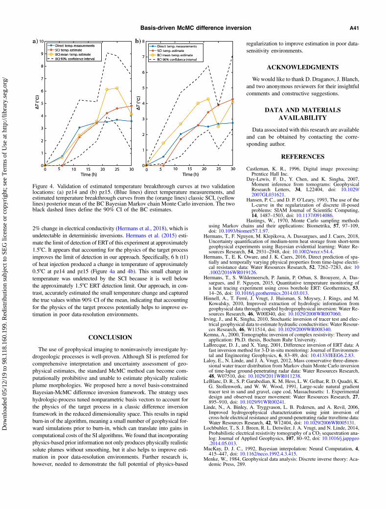
breakthrough curves at the two piezometers,pz14 and pz15, is presented in Figure 4. Bothstrategies accurately predicted the general tempo-ral behavior of the heat migration, with SCIout performing or underperforming our strategyat certain time steps. The 90% confidence interval(CI) of the estimates from our approach capturedalmost all of the true temperature measurements.In the data presented, a change of 1°C produced a
Figure 2. Sampling paths of (a) negative log-likelihood to deter-mine the burn-in period and (b) correlation coefficient for autocor-relation analysis.
Figure 3. Difference thermograms recovered from the ERT measurements at three dif-ferent time-steps: (row 1) 12 h, (row 2) 21.5 h, and (row 3) 30 h. Column (a) showstomograms from the classic SCI, columns (b–e) show, respectively, two posterior real-izations, posterior mean and standard deviations from the BC Bayesian Markov chainMonte Carlo difference inversion. The pz14 and pz15 are, respectively, located at (1.125,9 m) and (2.25, 8.5 m).
A40 Oware et al.
Dow
nloa
ded
05/1
2/19
to 9
8.11
8.16
0.19
9. R
edis
trib
utio
n su
bjec
t to
SEG
lice
nse
or c
opyr
ight
; see
Ter
ms
of U
se a
t http
://lib
rary
.seg
.org
/
2% change in electrical conductivity (Hermans et al., 2018), which isundetectable in deterministic inversions. Hermans et al. (2015) esti-mate the limit of detection of ERTof this experiment at approximately1.5°C. It appears that accounting for the physics of the target processimproves the limit of detection in our approach. Specifically, 6 h (t1)of heat injection produced a change in temperature of approximately0.5°C at pz14 and pz15 (Figure 4a and 4b). This small change intemperature was undetected by the SCI because it is well belowthe approximately 1.5°C ERT detection limit. Our approach, in con-trast, accurately estimated the small temperature change and capturedthe true values within 90% CI of the mean, indicating that accountingfor the physics of the target process potentially helps to improve es-timation in poor data-resolution environments.
CONCLUSION
The use of geophysical imaging to noninvasively investigate hy-drogeologic processes is well-proven. Although SI is preferred forcomprehensive interpretation and uncertainty assessment of geo-physical estimates, the standard McMC method can become com-putationally prohibitive and unable to estimate physically realisticplume morphologies. We proposed here a novel basis-constrainedBayesian-McMC difference inversion framework. The strategy useshydrologic-process tuned nonparametric basis vectors to account forthe physics of the target process in a classic difference inversionframework in the reduced dimensionality space. This results in rapidburn-in of the algorithm, meaning a small number of geophysical for-ward simulations prior to burn-in, which can translate into gains incomputational costs of the SI algorithms. We found that incorporatingphysics-based prior information not only produces physically realisticsolute plumes without smoothing, but it also helps to improve esti-mation in poor data-resolution environments. Further research is,however, needed to demonstrate the full potential of physics-based
regularization to improve estimation in poor data-sensitivity environments.
ACKNOWLEDGMENTS
Wewould like to thank D. Draganov, J. Blanch,and two anonymous reviewers for their insightfulcomments and constructive suggestions.
DATA AND MATERIALSAVAILABILITY
Data associated with this research are availableand can be obtained by contacting the corre-sponding author.
REFERENCES
Castleman, K. R., 1996, Digital image processing:Prentice Hall Inc.
Day-Lewis, F. D., Y. Chen, and K. Singha, 2007,Moment inference from tomograms: GeophysicalResearch Letters, 34, L22404, doi: 10.1029/2007GL031621.
Hansen, P. C., and D. P. O’Leary, 1993, The use of theL-curve in the regularization of discrete ill-posedproblems: SIAM Journal of Scientific Computing,14, 1487–1503, doi: 10.1137/0914086.
Hastings, W., 1970, Monte Carlo sampling methodsusing Markov chains and their applications: Biometrika, 57, 97–109,doi: 10.1093/biomet/57.1.97.
Hermans, T., F. Nguyen, M. Klepikova, A. Dassargues, and J. Caers, 2018,Uncertainty quantification of medium-term heat storage from short-termgeophysical experiments using Bayesian evidential learning: Water Re-sources Research, 54, 2931–2948, doi: 10.1002/wrcr.v54.4.
Hermans, T., E. K. Oware, and J. K. Caers, 2016, Direct prediction of spa-tially and temporally varying physical properties from time-lapse electri-cal resistance data: Water Resources Research, 52, 7262–7283, doi: 10.1002/2016WR019126.
Hermans, T., S. Wildemeersch, P. Jamin, P. Orban, S. Brouyere, A. Das-sargues, and F. Nguyen, 2015, Quantitative temperature monitoring ofa heat tracing experiment using cross borehole ERT: Geothermics, 53,14–26, doi: 10.1016/j.geothermics.2014.03.013.
Hinnell, A., T. Ferré, J. Vrugt, J. Huisman, S. Moysey, J. Rings, and M.Kowalsky, 2010, Improved extraction of hydrologic information fromgeophysical data through coupled hydrogeophysical inversion: Water Re-sources Research, 46, W00D40, doi: 10.1029/2008WR007060.
Irving, J., and K. Singha, 2010, Stochastic inversion of tracer test and elec-trical geophysical data to estimate hydraulic conductivities: Water Resour-ces Research, 46, W11514, doi: 10.1029/2009WR008340.
Kemna, A., 2000, Tomographic inversion of complex resistivity: Theory andapplication: Ph.D. thesis, Bochum Ruhr University.
LaBrecque, D. J., and X. Yang, 2001, Difference inversion of ERT data: Afast inversion method for 3-D in-situ monitoring: Journal of Environmen-tal and Engineering Geophysics, 6, 83–89, doi: 10.4133/JEEG6.2.83.
Laloy, E., N. Linde, and J. A. Vrugt, 2012, Mass conservative three-dimen-sional water tracer distribution from Markov chain Monte Carlo inversionof time-lapse ground-penetrating radar data: Water Resources Research,48, W07510, doi: 10.1029/2011WR011238.
LeBlanc, D. R., S. P. Garabedian, K. M. Hess, L. W. Gelhar, R. D. Quadri, K.G. Stollenwerk, and W. W. Wood, 1991, Large-scale natural gradienttracer test in sand and gravel, cape cod, Massachusetts: 1. Experimentaldesign and observed tracer movement: Water Resources Research, 27,895–910, doi: 10.1029/91WR00241.
Linde, N., A. Binley, A. Tryggvason, L. B. Pedersen, and A. Revil, 2006,Improved hydrogeophysical characterization using joint inversion ofcross-hole electrical resistance and ground-penetrating radar traveltime data:Water Resources Research, 42, W12404, doi: 10.1029/2006WR005131.
Lochbuhler, T., S. J. Breen, R. L. Detwiler, J. A. Vrugt, and N. Linde, 2014,Probabilistic electrical resistivity tomography of a CO2 sequestration ana-log: Journal of Applied Geophysics, 107, 80–92, doi: 10.1016/j.jappgeo.2014.05.013.
MacKay, D. J. C., 1992, Bayesian interpolation: Neural Computation, 4,415–447, doi: 10.1162/neco.1992.4.3.415.
Menke, W., 1984, Geophysical data analysis: Discrete inverse theory: Aca-demic Press, 289.
Figure 4. Validation of estimated temperature breakthrough curves at two validationlocations: (a) pz14 and (b) pz15. (Blue lines) direct temperature measurements, andestimated temperature breakthrough curves from the (orange lines) classic SCI, (yellowlines) posterior mean of the BC Bayesian Markov chain Monte Carlo inversion. The twoblack dashed lines define the 90% CI of the BC estimates.
Metropolis, N., A. Rosenbluth, M. Rosenbluth, A. Teller, and E. Teller,1953, Equation of state calculations by fast computing machines: Journalof Chemical Physics, 21, 1087–1092, doi: 10.1063/1.1699114.
Oware, E. K., 2016, Estimation of hydraulic conductivities using higher-or-der MRF-based stochastic joint inversion of hydrogeophysical measure-ments: The Leading Edge, 35, 776–785, doi: 10.1190/tle35090776.1.
Oware, E. K., M. Awatey, T. Hermans, and J. Irving, 2018, Basis-constrained Bayesian-McMC: Hydrologic process parameterization of sto-chastic geoelectrical imaging of solute plumes: 88th Annual InternationalMeeting, SEG, Expanded Abstracts, 5472–5476, doi: 10.1190/segam2018-w12-01.1.
Oware, E. K., and S. M. J. Moysey, 2014, Geophysical evaluation of soluteplume spatial moments using an adaptive POD algorithm for electricalresistivity imaging: Journal of Hydrology, 517, 471–480, doi: 10.1016/j.jhydrol.2014.05.054.
Oware, E. K., S. M. J. Moysey, and T. Khan, 2013, Physically based regu-larization of hydrogeophysical inverse problems for improved imaging of
process-driven systems: Water Resources Research, 49, 6238–6247, doi:10.1002/wrcr.20462.
Ruggeri, P., J. Irving, and K. Holliger, 2015, Systematic evaluation ofsequential geostatistical resampling within MCMC for posterior samplingof near-surface geophysical inverse problems: Geophysical JournalInternational, 202, 961–975, doi: 10.1093/gji/ggv196.
Satija, A., and J. Caers, 2015, Direct forecasting of subsurface flow responsefrom non-linear dynamic data by linear least-squares in canonical func-tional principal component space: Advances in Water Research, 77,69–81, doi: 10.1016/j.advwatres.2015.01.002.
Singha, K., F. D. Day-Lewis, T. Johnson, and L. D. Slater, 2015, Advance inthe interpretation of subsurface processes with time-lapse electrical imag-ing: Hydrological Processes, 29, 1549–1576, doi: 10.1002/hyp.v29.6.
Tarantola, A., 2005, Inverse problem theory and methods for model param-eter estimation: SIAM.
Tikhonov, A. N., and V. Y. Arsenin, 1977, Solutions of ill-posed problems:John Wiley and Sons.