Batch Emulsification Using an Inline Rotor-Stator in a Recycle Loop of Varying Volume A dissertation submitted to the University of Manchester for the degree of M.Sc. in the Faculty of Engineering and Physical Sciences 2009 JONATHAN PAUL MANNING SCHOOL OF CHEMICAL ENGINEERING AND ANALYTICAL SCIENCE
Transcript
Batch Emulsification Using an Inline
Rotor-Stator in a Recycle Loop of
Varying Volume
A dissertation submitted to the University of Manchester for the degree of
M.Sc. in the Faculty of Engineering and Physical Sciences
1.1. THE SCOPE OF THIS WORK .................................................................................................................... 9
2. LITERATURE REVIEW ........................................................................................................................ 11
2.1. MIXING FIELD THEORY ....................................................................................................................... 11 2.2. BATCH EMULSIFICATION ................................................................................................................... 12 2.2.1. THEORETICAL MODELLING ............................................................................................................ 13 2.2.2. EXPERIMENTAL INVESTIGATION .................................................................................................... 14 2.2.3. THE NEED TO INCLUDE THE RECYCLE LOOP VOLUME .................................................................... 16 2.3. EXPERIMENTAL CONSIDERATIONS ..................................................................................................... 16 2.3.1. PHYSICAL PROPERTIES OF EMULSIONS .......................................................................................... 16 2.3.2. TALL TANKS ................................................................................................................................... 17 2.3.3. PIPEWORK ...................................................................................................................................... 18 2.3.4. ROTOR STATORS ............................................................................................................................ 20 2.4. GENERAL THEORY OF DROPLET DISPERSION ...................................................................................... 22 2.4.1. KOLMOGOROV TURBULENCE ......................................................................................................... 22 2.4.2. HINZE THEORY OF INVISCID DROPLET STABILITY .......................................................................... 24 2.4.3. OBSERVATIONS OF DROPLET BREAKUP IN NON-ISOTROPIC TURBULENCE ..................................... 26 2.4.4. CORRELATING DROPLET SIZE IN STIRRED TANKS .......................................................................... 26 2.4.5. THE EFFECT OF SURFACTANT ......................................................................................................... 27 2.4.6. THE EFFECT OF DISPERSED PHASE FRACTION ................................................................................ 28 2.4.7. THE EFFECT OF DISPERSED PHASE VISCOSITY ................................................................................ 29 2.4.8. DISPERSION IN PIPES ...................................................................................................................... 32 2.5. ANALYSING DROP SIZE DISTRIBUTIONS ............................................................................................. 32 2.6. POPULATION BALANCES .................................................................................................................... 36 2.7. SUMMARY .......................................................................................................................................... 38
3. MODELLING THE RECYCLE LOOP VOLUME ............................................................................ 39
3.1. GENERAL ASSUMPTIONS .................................................................................................................... 39 3.2. PLUG FLOW IN THE RECYCLE LOOP .................................................................................................... 39 3.2.1. SPECIFIC ANALYTICAL SOLUTIONS ................................................................................................ 40 3.2.2. GENERAL FORM OF SOLUTIONS ..................................................................................................... 43 3.2.3. NUMERICAL SOLUTION .................................................................................................................. 45 3.3. LAMINAR FLOW IN THE RECYCLE LOOP .............................................................................................. 45 3.4. COMBINING PIPE SECTIONS. ............................................................................................................... 47 3.5. ADAPTATIONS FOR SEMI-BATCH OPERATION ................................................................................... 47 3.6. DISTRIBUTIVE MIXING ....................................................................................................................... 47 3.7. EXAMPLES .......................................................................................................................................... 48 3.7.1. CHARACTERISTIC PROFILE ............................................................................................................. 49 3.7.2. NARROWER DROP SIZE DISTRIBUTION ........................................................................................... 50
3
3.7.3. IMPACT ON SCALE UP CALCULATIONS ........................................................................................... 50 3.7.4. THE EFFECT OF DECREASING TANK VOLUME ................................................................................. 52 3.7.5. DISTRIBUTIVE MIXING .................................................................................................................. 53 3.8. A POTENTIAL IMPROVEMENT TO CURRENT INDUSTRIAL PRACTICE ................................................... 54 3.9. SUMMARY .......................................................................................................................................... 55
4. MODELLING THE EFFECT OF THE INLINE MIXER ................................................................. 56
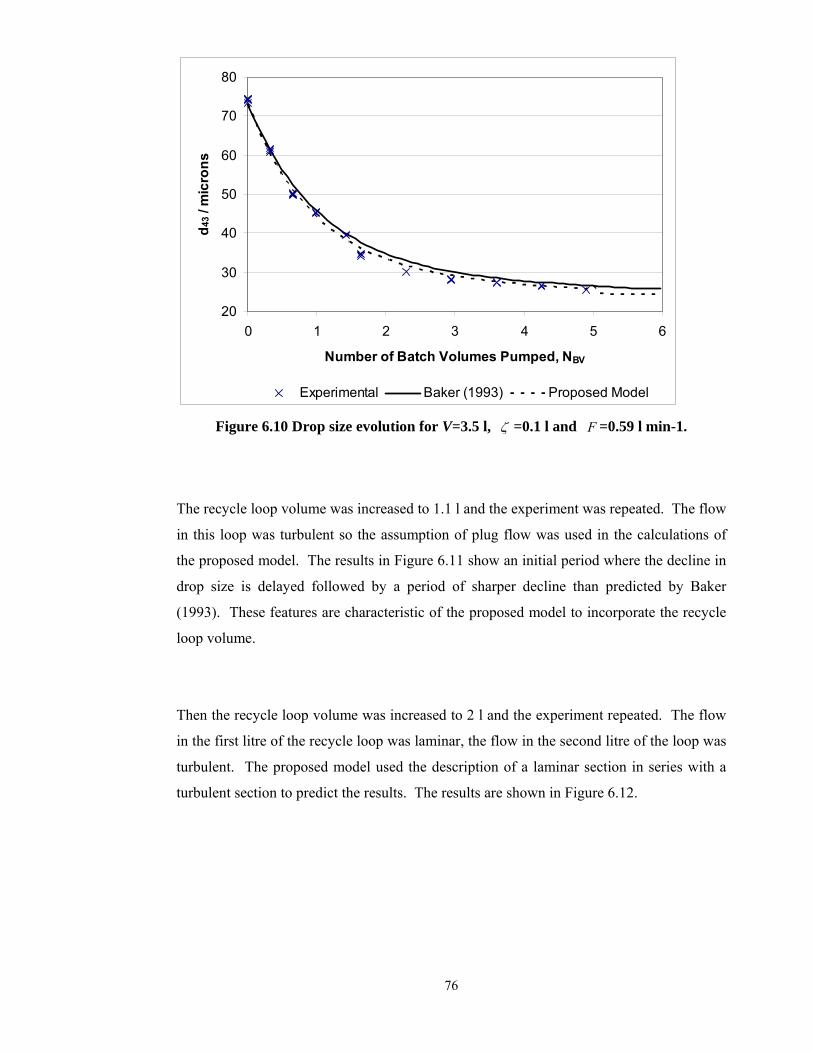
6.1. CALIBRATION OF PUMP SPEED ............................................................................................................ 67 6.2. PREPARATION OF AN INITIAL, COARSE EMULSION ............................................................................. 67 6.3. INVESTIGATION OF THE MIXING TIME IN THE STIRRED TANK ............................................................. 69 6.4. TEST OF THE VOLUME AVERAGING TECHNIQUE ................................................................................. 70 6.5. CALIBRATION OF THE SENSORS ON THE INLINE MIXER ...................................................................... 71 6.6. CHARACTERISING THE INLINE MIXER ................................................................................................. 71 6.7. EMULSIFICATION USING AN INLINE MIXER IN A RECIRCULATION LOOP OF FINITE VOLUME. ............. 74 6.8. SUMMARY .......................................................................................................................................... 80
7.1. THE VARIATION IN INITIAL DROP SIZE ................................................................................................ 81 7.2. STABILITY OF THE RECYCLE LOOP FLOWRATE ................................................................................... 83 7.3. VALIDITY OF THE VOLUME AVERAGING TECHNIQUE ......................................................................... 83 7.4. ASSESSING THE THEORETICAL MODELS ............................................................................................. 84 7.5. CHARACTERISING THE INLINE MIXER ................................................................................................ 85 7.6. SUMMARY .......................................................................................................................................... 90
8.1. THE EFFECT OF RECYCLE LOOP VOLUME ............................................................................................ 91 8.2. EXPERIMENTAL VALIDATION OF THE MODEL ..................................................................................... 91 8.3. CHARACTERISING THE DISPERSION .................................................................................................... 92 8.4. RECOMMENDATIONS FOR FURTHER WORK ........................................................................................ 93
Figure 2.1 Showing the equipment for Batch Recirculation Emulsification (Taken from Baker 1993) ...................................................................................................................................... 12 Figure 3.1 Schematic diagram of the system being modelled. ......................................................... 40 Figure 3.2 Comparing the Evolution of C0 Predicted by Different Models. ..................................... 49 Figure 3.3 Comparing predicted distributions of Ci for different models. ........................................ 50 Figure 3.4 Showing the profile of 0C over time. ............................................................................. 52
Figure 3.5 Showing the distributions of iC at NBV=2 ....................................................................... 53
Figure 3.6 Showing the profile of φ with time ................................................................................ 53 Figure 3.7 Diagram of a Multi-Stage Mixing Tank (Hemrajani and Tatterson 2004) ..................... 54 Figure 5.1 Schematic diagram of the experimental equipment. Tank dimensions in mm ................ 59 Figure 5.2 Showing the dimensions of the impellers ........................................................................ 60 Figure 6.1 Showing the Sauter Mean Drop Diameter in the Stirred Tank Reducing With Time. ................................................................................................................................................. 68 Figure 6.2 Showing the variation in drop sizes between batches. ............................................... 69 Figure 6.3 Showing the Volume Fraction of the Cream Layer Over Time ............................... 70 Figure 6.4 Showing d43 for another mixture of two emulsions .................................................. 71 Figure 6.5 Showing the change in the drop size distribution after one pass through the inline mixer operating at 5000 rpm. ........................................................................................................ 72 Figure 6.6 The effect of the inline mixer operating at 5000 rpm ................................................ 73 Figure 6.7 Showing the effect of the inline mixer operating at 9300 rpm .................................. 73 Figure 6.8 The change in drop size distribution after 8 passes through the inline mixer operating at 9300 rpm. ................................................................................................................... 74 Figure 6.9 Drop size evolution for V =3.5 l, ζ =0.1 l and F =0.9 l min-1. .............................. 75 Figure 6.10 Drop size evolution for V=3.5 l, ζ =0.1 l and F =0.59 l min-1. ............................ 76 Figure 6.11 Drop size evolution for V=3.0 l, ζ =1.1 l and F =0.68 l min-1 ............................. 77 Figure 6.12 Drop size evolution for V=3.5 l, ζ =2 l and F =0.63 l min-1 ................................ 77 Figure 6.13 Drop size evolution for V=3.5 l, ζ =3 l and F =0.591 l min-1 ............................... 78 Figure 6.14 Drop size evolution for V=3.5 l, ζ =3 l and F =0.812 l min-1 ............................... 79 Figure 6.15 Drop size evolution for V=3.5 l, ζ =3 l and F =0.810 1 l min-1 ........................... 79 Figure 7.1 Similarity test for dispersion in the stirred tank. ....................................................... 86 Figure 7.2 The breakage matrix characterising the effect of the Silverson Mixer operating at 9300 rpm .......................................................................................................................................... 87 Figure 7.3 Predicted and observed drop size distributions after passing a batch twice through the inline mixer operating at 9300 rpm. ........................................................................................ 88 Figure 7.4 The daughter droplet distribution for parent droplets between 80-100 µm ........... 89
LIST OF TABLES
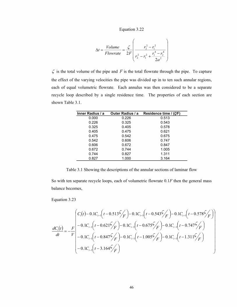
Table 3.1 Showing the descriptions of the annular sections of laminar flow ................................... 46 Table 6.1 Showing the average values of d43(i) ............................................................................. 74
5
Abstract
In industry emulsions are produced by recirculating the contents of a stirred tank through
an inline mixer located in a recycle loop. The distribution of drop sizes in the stirred tank
depends on the number of batch volumes, BVN , that have been pumped around the loop.
When scaling up pilot trials the value of BVN is kept constant. One factor that changes
between these scales is the size of the recycle loop relative to the size of the tank. The
effect of this factor is unknown since existing models neglect the volume of the recycle
loop.
This study extends an existing model of Baker (1993) to include the effect of a finite
residence time in the recycle loop. Larger loop volumes are shown to lead to narrower
distributions within the stirred tank and more rapid reduction of the fraction that has not
passed through the mixer. On scaling up to industrial scales the recycle loop normally
becomes proportionally smaller. Consequently if BVN is held constant the results will not
be as good as the trials: the distribution will be wider and less material will have passed
through the mixer at least once.
An experimental study was conducted to investigate these predictions. At small recycle
loop volumes the results from the literature were accurately reproduced. At larger recycle
loop volumes it was possible to detect characteristic features of this extended model.
However the shortcomings of the available inline mixer limited the contrast between the
existing model and the proposed extension.
A rotor-stator was used as the inline mixer. A new method of representing the dispersive
process as a matrix transformation has been developed. This allowed determination of the
daughter droplet distributions without a priori assumptions of their form. These have been
shown to be broader than the distributions normally assumed in the literature.
6
Declaration I declare that no portion of the work referred to in the dissertation has been submitted in
support of an application for another degree or qualification of this or any other university
of other institute of learning.
Jonathan Manning
Copyright Statement
i. Copyright in text of this dissertation rests with the author. Copies (by any process)
either in full, or of extracts, may be made only in accordance with instructions
given by the author. Details may be obtained from the appropriate Graduate
Office. This page must form part of any such copies made. Further copies (by any
process) of copies made in accordance with such instructions may not be made
without the permission (in writing) of the author.
ii. The ownership of any intellectual property rights which may be described in this
dissertation is vested in the University of Manchester, subject to any prior
agreement to the contrary, and may not be made available for use by third parties
without the written permission of the University, which will prescribe the terms and
conditions of any such agreement.
iii. Further information on the conditions under which disclosures and exploitation
may take place is available from the head of the School of Chemical Engineering
and Analytical Science.
7
Acknowledgments
I am very grateful to my supervisor Dr. Peter Martin for his direction which focussed my experimental work and our discussions that developed my thinking.
Many thanks also to :
Adam Kowalski of Unilever for the generous loan of the Silverson mixer used in these experiments.
Craig Shore for skilfully fitting the equipment and his practical troubleshooting.
Dr. Mike Cooke for his help with matters practical and theoretical.
Liz Davenport and Eric Warburton for their patient help with the Mastersizer.
8
1. Introduction
Recycle loop volume: an unknown factor in the scale up of batch
emulsification processes
The fine chemicals industry is characterised by a need for continual product development
to maintain commercial advantages. This requires experimentation at laboratory and pilot
plant scales. The results then need to be scaled up to industrial capacities. The process of
scale up is fraught with difficulty and small errors at the trial stage can be magnified
significantly. The annual cost of failed mixing scale up in the US alone is estimated to be
$10 billion (Kresta et al 2004). In batch emulsification processes the finished product is
made by recycling the contents of a stirred tank through an inline mixer. The resulting
distribution inside the stirred tank is modelled in the literature (Baker 1993). Baker
showed that at any time some of the material in the stirred tank will not have passed
through the inline mixer whilst some will have passed through many times. This leads to
wide drop size distribution. By calculating how much material has been through the mixer
at any number of times Baker was able to predict how the drop size in the stirred tank
evolved with time. Industrial processes are designed using the results of this model
(Brocart et al 2002). However Baker’s model neglects the volume of the recycle loop.
The relative volume of the recycle loop compared to the batch volume is something that
varies with scale. Because this has not been considered there is no understanding of how
this impacts on the result of scale up. Small uncertainties at laboratory scale trials can cost
millions of dollars at the industrial scale (Cohen 2005). Therefore it is very important that
this effect be quantified. More reliable scale up will reduce the lead times for developing
new products and reduce the risk of losses due to failure to produce the right quality of
product.
The properties of emulsions and dispersions prepared in this way are dependent on the
particle size distributions. For example clay filler can be added to asphalt to prepare a road
surface layer (Cohen 2005). The value of this layer lies in its thixotropic rheology and this
requires very thorough dispersion of the clay particles. Production of polymers via free
radical polymerisation in colloidal dispersions is another example. In a polymerization
reaction the ratio between Laplace pressure and osmotic pressure depends on drop size (El-
Jaby et al 2007). A wide drop size distribution would lead to a wide range of reaction rates
which would be undesirable. Clearly product design is related to controlling the drop size
distribution. By understanding the impact of the recycle loop volume on the drop size
distribution it will be possible to more accurately control the properties of these products.
9
The equipment used to make these products is not well understood. There is great secrecy
around the performance of the rotor-stator mixers that are used to disperse the emulsions.
The manufacturers maintain their competitive advantage by keeping a close guard on
research data. There is not much publicly available information on their performance or
how to scale up to larger mixers. There are many factors used to scale up rotor stator
processes and the overall picture is confused. The voice of industry is clear that the
procedure is, “more art than science,” (Ryan and Thapar 2009), “often doesn’t turn out as
planned,” (Shelley 2004) and is generally achieved through “trial and error,” (D’Aquino
2004). The list of relevant factors is long and some are contradictory. Successful process
design requires the selection of the most appropriate mixer for the job but this is not always
straightforward: proprietary application guidelines for commercial mixers are a closely
guarded secret (Cohen 2005); there is “almost no fundamental basis” to predict the
performance of given design (Shelley 2004). Many experimental tests are “purely
subjective” making definitive comparisons between different pieces of equipment very
difficult (Ryan and Thepar 2008). These factors serve to hinder the development of new
processes.
1.1. The scope of this work A survey of the literature examines how the batch emulsification process has been
modelled by neglecting the recycle loop volume. An experimental procedure for testing
the model is critically assessed. This provides the background for modelling the effect of
recycle loop volume and investigating the predictions. The issues relating to particular
items of equipment are considered to aid the design of an experimental rig. The theoretical
understanding of the dispersive process is examined. This allows consideration of the
extent to which the existing methods can be applied to characterise rotor-stators.
The model in the literature is extended to include the effect of the recycle loop volume. To
check its validity the solutions for a system with very small recycle loop volume are
compared to the existing solutions from the literature. The characteristic effects of this
new model are then identified. Example calculations show the significance of the findings
for successful scale up and process development.
The experimental method outlined in the literature (Baker 1993) has been improved and
applied to test the predictions of this new model. Comparison is made with the predictions
of the existing model.
Finally a new concept of representing the effect of the inline mixer as a matrix
transformation is investigated. This is shown to be an accurate model of the process. The
10
resulting matrix gives details of the daughter droplet distribution and breakage function
that would not have been accessible through standard application of population balance
models.
11
2. Literature Review The primary aim of this work is to understand the effect of the recycle loop volume in
batch emulsification systems. By reviewing how mixing field theory has been applied to
analyse the process it is possible to see how to extend the existing model. The
experimental system of Baker (1993) is the basis of the method followed here so it was
important to review those techniques. When designing the experimental rig it is important
to be able to relate the properties of the equipment to the assumptions in the model so some
general issues around these items are investigated. In order to achieve the secondary aim
of characterising the inline mixer it is important to understand how previous studies have
tackled similar problems. This reveals the assumptions that are made and assesses whether
they apply to rotor-stators or not. Finally, population balances have been used successfully
to model dynamic dispersion processes. It is worthwhile to consider the strengths and
weaknesses of this approach to the current problem.
2.1. Mixing field theory The fine chemicals industry is driven by product innovation. A new formulation will have
to meet certain specifications such as stability or sensory feel to be acceptable to the
market. In practical terms these requirements may be expressed as constraints on average
drop size or the drop size distribution (Brocart et al 2002). Experiments at the laboratory
and pilot scales are necessary to determine how to achieve these goals. These results must
then be scaled up to full size for a successful process. A recent review of mixing research
explains how a proper understanding of the process requirements improves the chances of
success at each stage . The old approach relied on design guidelines specific to each type
of equipment and was inflexible with regard to developments in technology or non-
standard mixing problems (Kresta et al 2004). The recommended alternative is to express
process requirements in terms of mixing fields. A mixing field is characterized by the
intensity of mixing and the residence time of a fluid element in the field. By similarly
describing available equipment in terms of the mixing field produced it is possible to
design the process by matching the requirements with the characteristics of appropriate
mixers. Scaling up the equipment becomes a question of achieving the same mixing field
at a larger scale. Kresta et al (2004) give the example of a stirred tank which can be
modeled as containing two mixing zones: the impeller region where intensity is high but
residence time low; and the bulk of the vessel where mixing intensity is of the order of 100
times lower but the residence time is longer. A crystallization process is cited as an
example where this description is used with very good success. If the selectivity of a
reaction is known to be controlled by micro-mixing then this determines the mixing
12
requirements: a mixing zone of high intensity. Such reactions are rapid so a short
residence time in this zone is unlikely to be a problem. Comparison of the process
requirements with the equipment properties shows that a stirred tank will satisfy the
requirements if the reactant is fed directly to the impeller zone.
2.2. Batch Emulsification A similar approach is used to analyse the process of manufacturing emulsions. The
required mixing duty can be decoupled in to two parts: dispersive and distributive (Baker
1993). Distributive mixing refers to the blending requirement whereby the separate
components of a mixture are to be distributed evenly throughout a product. Dispersive
mixing is the breakup of the dispersed phase droplets to smaller sizes. This might be to
increase the rate of mass transfer between the phases or to stabilize the emulsion if it is the
end product. Stirred vessels are readily available in the fine chemicals industry due to their
versatility. They can supply a mixing field capable of meeting the distributive needs but
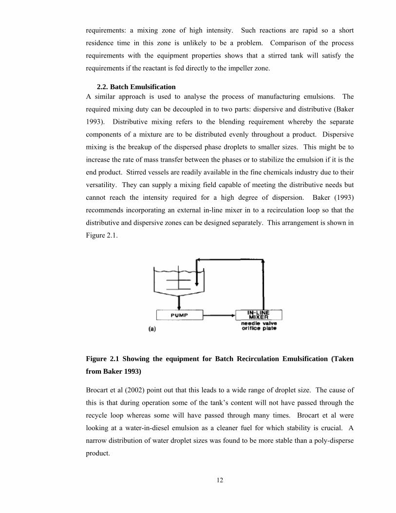
cannot reach the intensity required for a high degree of dispersion. Baker (1993)
recommends incorporating an external in-line mixer in to a recirculation loop so that the
distributive and dispersive zones can be designed separately. This arrangement is shown in
Figure 2.1.
Figure 2.1 Showing the equipment for Batch Recirculation Emulsification (Taken
from Baker 1993)
Brocart et al (2002) point out that this leads to a wide range of droplet size. The cause of
this is that during operation some of the tank’s content will not have passed through the
recycle loop whereas some will have passed through many times. Brocart et al were
looking at a water-in-diesel emulsion as a cleaner fuel for which stability is crucial. A
narrow distribution of water droplet sizes was found to be more stable than a poly-disperse
product.
13
2.2.1. Theoretical modelling Clearly then it is a matter of practical importance to determine the fraction which has not
passed through the loop and that which has passed through any given number of times.
Baker (1993) shows how this can be done by using a model with two assumptions: the
stirred tank is well mixed and the volume of the recycle loop is negligible. The initial
condition is that at time t=0 then C0=1 where C0 is the volume fraction in the tank that has
not passed through the inline mixer. The assumption of a well mixed tank leads to a mass
balance on C0 of
Equation 2.1
00 C
VF
dtdC
−=
Where F is the flowrate round the recycle loop and V is the volume of the tank. The
solution is
Equation 2.2
BVNVFt
eeC −−
==0
Where VFtNBV = is the number of batch volumes that have been pumped round the recycle
loop. In general Ci is the volume fraction in the tank that has passed through the inline
mixer i times and the relevant mass balance is (Baker 1993),
Equation 2.3
( )iii CC
VF
dtdC
−= '
'iC is the volume fraction of the material returning to the tank that has passed through the
inline mixer i times. By neglecting the recycle loop volume the material is assumed to take
no time to pass through the loop which leads to the identification,
Equation 2.4
1'
−= ii CC
Using this relationship to solve Equation 2.3 Baker (1993) found the general solution to be,
14
Equation 2.5
!iNe
CiN
iBV
BV−
=
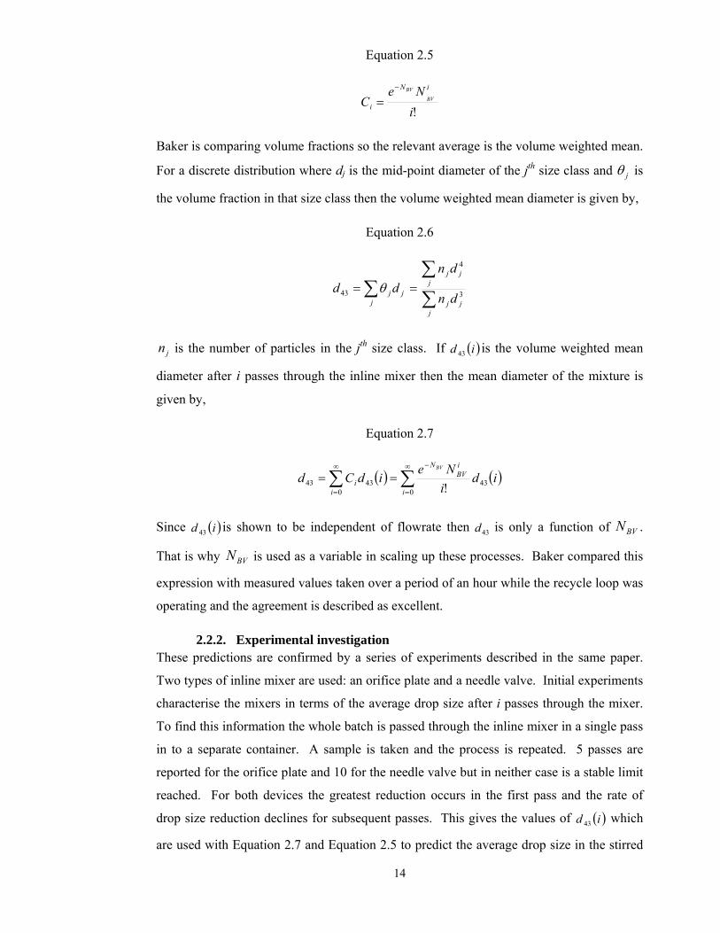
Baker is comparing volume fractions so the relevant average is the volume weighted mean.
For a discrete distribution where dj is the mid-point diameter of the jth size class and jθ is
the volume fraction in that size class then the volume weighted mean diameter is given by,
Equation 2.6
∑∑
∑ ==
jjj
jjj
jjj dn
dndd 3
4
43 θ
jn is the number of particles in the jth size class. If ( )id 43 is the volume weighted mean
diameter after i passes through the inline mixer then the mean diameter of the mixture is
given by,
Equation 2.7
( ) ( )∑∑∞
=
−∞
=
==0
430
4343 !i
iBV
N
ii id
iNe
idCdBV
Since ( )id 43 is shown to be independent of flowrate then 43d is only a function of BVN .
That is why BVN is used as a variable in scaling up these processes. Baker compared this
expression with measured values taken over a period of an hour while the recycle loop was
operating and the agreement is described as excellent.
2.2.2. Experimental investigation These predictions are confirmed by a series of experiments described in the same paper.
Two types of inline mixer are used: an orifice plate and a needle valve. Initial experiments
characterise the mixers in terms of the average drop size after i passes through the mixer.
To find this information the whole batch is passed through the inline mixer in a single pass
in to a separate container. A sample is taken and the process is repeated. 5 passes are
reported for the orifice plate and 10 for the needle valve but in neither case is a stable limit
reached. For both devices the greatest reduction occurs in the first pass and the rate of
drop size reduction declines for subsequent passes. This gives the values of ( )id 43 which
are used with Equation 2.7 and Equation 2.5 to predict the average drop size in the stirred
15
tank. After this data has been found pilot scale batch emulsifications are performed. The
recycle loop returns the processed emulsion to the stirred tank and the drop size is
measured at different times. The predictions of Baker’s model provide a good fit to the
measured data and confirm the theoretical model.
Baker is able to further validate his model by looking at the evolution of the drop size
distribution. The distributions after i passes can be combined, weighted with the values of
iC , to predict the distribution after a given time. The results are very clear and support his
conclusion. This is helped because his inline mixers produce an order of magnitude
change in drop size. In systems where less drastic changes are produced then the evolution
of the drop size distribution might be less easy to discern with the naked eye.
A similar experimental investigation is necessary for the present work so it is important to
recognize some problems with Baker’s method. To create an initial emulsion in the stirred
tank Baker pours the oil phase on to the surface of the aqueous phase. This is not an
efficient way of mixing the phases (El-Hamouz et al 2009) as it can lead to large droplets
staying on the surface and not being entrained in to the bulk. More seriously he defines
0=t at the moment the oil is poured on to the surface. There are many studies showing
that in a stirred tank the equilibrium drop size is not reached until a period of the order of 1
hour (Pacek et al 1998, Calabrese et al 1986a, Arai et al 1977). Application of Equation
2.7 implicitly assumes that ( )043d is constant i.e. that there is no drop breakup in the tank.
This will not be true in Baker’s experiment. The reason that his results are not
compromised is that his inline mixer achieves almost an order of magnitude reduction in
drop size. The effect of the inline mixer outweighs the marginal decline in ( )043d with
time. An additional consequence of both these problems is the variation in ( )043d between
batches. (NB- Baker prepares a master batch of each phase to ensure consistency but for
each experiment a new batch of emulsion is created in the tank and this is the batch
referred to here.) This in itself might not be a problem but it is not clear that Baker is
consistent in addressing it. In Baker (1993) the values of ( )id 43 are reported for both the
orifice plate and the needle valve. The ( )043d value for the orifice plate is ~50 μm and for
the needle valve it is less than 40 μm. This is not consistent with his comparison between
the predictions of Equation 2.7 and his experimental results. In this case he uses ( )043d
=50 μm for both cases. The fit looks like it would be improved if the value of 40 μm were
to be used for the needle valve. Because of this it seems likely that 40 μm would be the
correct value and that Baker has made an oversight. Again the effect is small in
16
comparison to the large change due to the inline mixer so it does not affect his conclusion.
In future work attention should be paid to this point.
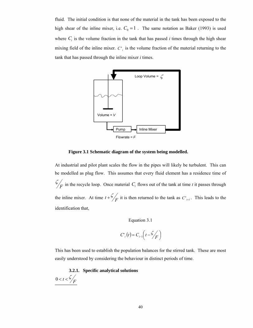
2.2.3. The need to include the recycle loop volume The setup shown in Figure 2.1 represents the simplest case. In industrial applications it is
sometimes necessary to incorporate an additional loop around the inline mixer (Brocart et
al 2002). This effectively increases the residence time in the high shear mixing field. If
the residence time is increased significantly then the assumption of a negligible residence
time will become invalid.
2.3. Experimental considerations In order to commission an experimental rig to perform a similar investigation it is
necessary to consider the properties of the available equipment. Batch emulsification
requires a stirred tank, an inline mixer, a pump and pipework connecting it all together. In
addition the physical properties of the emulsion need to be considered when designing the
experiments.
2.3.1. Physical properties of emulsions The principle properties of interest for this experiment are the viscosity and resistance to
coalescence. These need to be known in order to calculate the flow regime in the pipes and
ensure that the emulsion is stable to match the assumptions of the theoretical model.
The viscosity of an emulsion is given by,
)5.21( φμμ += c
Where cμ is the continuous phase viscosity and φ is the dispersed phase volume fraction.
This has been successfully applied at phase fractions up to 10% so will cover the range
used in this work (Becher 2001).
The presence of surfactant reduces the interfacial tension and stabilises the emulsion. To
ensure the greatest reduction in interfacial tension it is necessary to use a surfactant
concentration above the critical micelle concentration (cmc). To eliminate the effect of
dynamic surface tension it is necessary to operate significantly above the cmc (Koshy et al
1988). As the oil droplets are dispersed the interfacial area increases. More surfactant will
adsorb at the interface and deplete the concentration in the bulk. This effect needs to be
accounted for. The surfactant used, SLES, has a cmc of 0.2 mmol l-1 and an average
molecular weight of 420 (El-Hamouz 2007). The head group for a range of surfactants
was found to occupy 0.6 nm2 at the interface (Goloub et al 2003). SLES was not one of
17
these surfactants but this will serve as a useful estimate. Using these values it is possible to
calculate the concentration of surfactant in the bulk. If the aqueous phase is 1% SLES by
weight, the dispersed phase fraction is 5 % by volume and the drop diameter is 1μm then
the concentration in the bulk will still be more than 100 times the cmc.
The surfactant ensures that the emulsion is stable against coalescence. The continuous
phase is not very viscous so the emulsion will be prone to creaming. This will not cause
any problems because the agitation in the stirred tank will be enough to keep the emulsion
well mixed.
2.3.2. Tall tanks For agitated tanks of standard geometry the blending process is well documented in
standard textbooks. For a non-standard geometry, such as a tall tank it is necessary to
confirm whether and under what conditions standard results apply. Then the equipment
can be evaluated to see if it matches the requirements.
The mixing regime is turbulent for tank Reynolds numbers of order 104 or more. For
geometrically similar tanks the product 95Nt is a constant (Miller 2009). Numerical
models incorporating turbulent mixing and flow patterns can be used to estimate 95t . The
tall tanks are modelled as consisting of several ideally mixed cells with intracellular flow
between adjoining cells. This is justified because the agitators are hydro-dynamically
distinct provided that they are sufficiently separated. The minimum separation is
interpreted differently by different studies: either twice the impeller diameter (Jahoda and
Machon 1994) or the tank diameter (Alves et al 1997). These are both the same order of
magnitude so there is a clear rule of thumb to estimate if this effect needs to be taken in to
account.
Jahoda and Machon (1994) found that for 2, 3 and 4 impellers the dimensionless mixing
times 95Nt were respectively ~80, 200 and 400. By comparison the study by Alves et al
(1997) found values of ~ 100 and 200 for 2 and 3 impellers respectively. In both cases the
results were independent of Reynolds number. Clearly the mixing time increases with the
number of stages due to the limited mass transfer between cells.
This effect may sometimes be desired and horizontal donut baffles can be added to reduce
mass transfer between the zones. If the flow in and out of the tank is at opposite ends then
4 to 6 of these zones create a very good approximation to plug flow (Hemrajani 2004).
This combination of mixing and plug flow has applications in many processes such as
extraction, dissolution and polymerization.
18
The effect of impeller geometry is not clear. Ranada et al (1991) claim that a downflow
pitched blade turbine is most efficient for liquid phase mixing. Jahoda and Machon (1994)
found that pitched blades are more efficient than Rushton turbines but that the direction of
impeller pumping did not affect the mixing time. From an experimental point of view the
most important thing is consistency so if pitched blades are used the direction of pumping
should be held constant.
In the context of a recirculating batch emulsification loop the main vessel will be
considered well mixed if the mixing time is short compared to the characteristic residence
time FV . The results above allow an order of magnitude estimate of the dimensionless
mixing time to be made for comparison. If there is large density difference between the
two phases of an emulsion the mixing times will be greater than these predictions.
2.3.3. Pipework Mixing occurs not only in the dedicated devices but also in the pipes as the fluid flows
through them. In order to incorporate the recycle loop volume in to Baker’s model it is
necessary to understand the mixing field in the pipe. Dispersive mixing is best considered
in the context of the general theory of dispersive mixing. In this section the distributive
mixing field will be examined and this depends on the flow regime.
Turbulent flow is the simplest case. Turbulent flow in pipes is generally modeled as plug
flow. Perfect radial mixing and a single residence time for all fluid elements are assumed.
The random eddies are responsible for the radial mixing and an empirical rule of thumb
states that this occurs over a pipe length approximately 100 times the pipe’s diameter
(Etchells and Meyer 2004). Since the eddies occur in all directions they also cause axial
mixing and it seems reasonable that axial mixing will occur at a similar rate to radial
mixing. This gives a very crude estimate that the length of axial mixing is 1/100th of the
pipe length. In terms of the residence time this is a variation of 1% so plug flow is a
reasonable assumption. However random walk processes proceed with the square root of
time so whilst this might be a useful first estimate it does not give a good understanding of
the phenomena. Soluble salts in turbulent water pipes diffuse with a virtual coefficient of
diffusion k given by (Taylor 1954),
*1.10 avDturbulent =
Where a is the pipe’s internal diameter and ρτWv =* is the wall friction velocity.
Taylor develops this approach to model how the interface between two elements of fluid
19
develops with time. The characteristic length of the axial mixing, S, in a pipe of length, L,
is given by (Taylor 1954)
Equation 2.8
uvaLS *4372 =
u is the mean velocity in the pipe. The formula matched experiments where two different
types of gasoline were pumped along the same pipe, one after the other.
This shows that it is reasonable to model the turbulent flow in a pipe as plug flow and that
the degree of deviation from this ideal can be readily estimated.
In laminar flow there is a strong variation in velocity over the cross section and fluid
elements follow the streamlines. This leads to a wide variation in residence times. For the
diffusion of soluble salts in laminar flow there are two regimes. If the molecular diffusion
is slow then the variation in residence times is determined by the radial velocity variations.
If molecular diffusion is fast then it leads to radial mixing in addition to the axial mixing.
Diffusion becomes important when (Taylor 1953a),
Equation 2.9
molDa
uL
2
2
0 8.3>>
Where 0u is the peak velocity in the pipe and molD is the molecular coefficient of diffusion.
In an emulsion the diffusion would be due to Brownian motion of the droplets. For this
process the coefficient of diffusion is (Becher 2001 p.74),
Equation 2.10
dTk
Dc
KelvinBBrownian πμ3
=
Bk is the Boltzmann constant, KelvinT the absolute temperature in degrees Kelvin, cμ is the
viscosity of the continuous phase and d is the droplet diameter. For droplets ~50 μm
across at room temperature suspended in water then,
1563
23
107.81050103
2981038.1 −−−
−
×=×××××
=πBrownianD
20
So for a pipe of radius 5mm diffusion will only become significant when the residence
time is greater than,
Equation 2.11
( ) 8152
23
102107.88.3
103×=
×××
−
−
s
The time constraints of a three month dissertation rule out an investigation of this regime
so diffusion in the pipes will be ignored.
The radial variation in velocity in laminar flow is then given by (Taylor 1953a),
Equation 2.12
( ) ( )22
0 1 aruru −=
This can be used to determine the residence time distribution if necessary.
The literature shows that plug flow is a reasonable model for turbulent flow in pipes. The
degree of axial mixing can be estimated to check whether it could affect the modelling. In
laminar flow the residence time distribution will need to be taken into account. This
information can be used to understand the effect of the recycle loop volume in batch
recirculation emulsification.
2.3.4. Rotor Stators Rotor-stators are used in industrial applications where high shear mixing is required.
Compared to conventional mechanical agitators they are not well understood. There has
been little fundamental research into them and commercial incentives mean that what work
is done is often not widely available. A review of some available scientific work and the
trade press reveals the current level of knowledge and suggests which areas would benefit
from further investigation.
The defining feature of a rotor-stator is a high speed rotor in close proximity to a stator.
The gap between rotor and stator is typically 100-3000 μm and rotor tip speeds are of the
order 10-50 m s-1 (Utomo et al 2009). The maximum shear stress is achieved in this gap
(Barailler et al 2006) and reaches values of 100,000 m s-1 (D’Aquino 2004). The stator
surrounds the rotor and is perforated with narrow openings, the exact size and shape of
which vary between designs. The agitated liquid flows through these holes as jets (Shelley
21
2004). The velocity of the jets is proportional to the rotor tip speed (Utomo et al 2009).
Computational fluid dynamics has been used to show that it is not the mechanical forces in
the shear gap that are responsible for dispersion (Barailler et al 2006). Rather dispersion
occurs in the jets discharged from the slots. The resulting flows are assumed to be highly
turbulent (Bourne and Studer 1992) and capable of providing high intensity mixing for a
variety of applications.
In assessing the level of turbulence in the rotor stator Barailler (2006) has pointed out that
the Reynolds number is ambiguous. By analogy with stirred tanks it could be defined,
μρ 2
ReND
=
But in the high shear region it could be defined,
μδρ gapND
=Re
Where gapδ is the width of the gap between rotor and stator. In addition when you
consider that turbulence in the jet region is responsible for dispersive mixing then a third
variation presents itself,
μρ NDb
=Re
Where b is the width of the hole in the stator. This might seem like splitting hairs but there
is at least an order of magnitude difference between each one.
Whilst the level of turbulence indicates the strength of the mixing field it is not very useful
for predicting performance. Specific power has been successfully used to correlate mixer
performance across a wide range of technologies (Davies 1987). The overall power
consumption in rotor stators is controlled by a power number as for standard agitators so,
Equation 2.13
ρ530 DNPP =
The rotation causes the mixer to act as a centrifugal pump. Typical of such pumps the
Power number is proportional to the flowrate (Utomo et al 2009). Typical values of the
power number are 3 (Barailler et al 2006) for a head made by VMI Rayneri (France) and
1.7-2.3 (Utomo et al 2009) for a Silverson L4RT, depending on the stator. The choice of
22
stator also affects the particle size distribution (Ryan and Thapar 2008). One possible
reason for this is that narrower slits have a more even distribution of ε across them and
this would cause a narrower drop size distribution. Brocart (2002) shows that the energy
dissipation rate in the stator hole is given by,
Equation 2.14
( )b
ND4
3ρε ≈
This is an interesting result since is predicts that the rotor stator’s performance should be
equally well correlated by tip speed or local energy dissipation rate.
Even if ε can be successfully used to correlate a rotor-stator’s performance it gives no
information about the breakage kinetics. There is a great need for an “underlying
mathematical representation to model and predict,” the operation of these mixers (Shelley
2004). The field of population balances has been applied to this end to investigate agitated
tanks and offers the opportunity to explain rotor-stators (Kowalski 2008). So in order to
better characterise rotor stators it is important to understand the work that has already been
done towards characterising stirred tanks.
2.4. General theory of droplet dispersion The break-up of droplets in high Reynolds number flows is caused by dynamic forces in
the continuous phase. These forces are resisted by the viscosity and surface tension of the
dispersed phase droplets. This process is most often explained in the literature in terms of
early work on the structure of turbulent flows and the deformation of drops that is
collectively known as the Kolmogorov-Hinze theory of droplet breakup.
2.4.1. Kolmogorov turbulence The fluid velocity at any point in turbulent flow may be thought of as having an average
value upon which is superimposed a random vector (Kolmogorov, 1941a). These random
eddies exist on a range of scales from the macroscopic scale of the equipment down.
Kolmogorov states that these macroscopic eddies absorb energy from the fluid motion and
pass it on in turn to smaller scale eddies. This energy transfer is achieved through a
process called vortex stretching (Baldyga and Bourne, 1999, p62). Velocity fluctuations in
one direction create smaller velocity fluctuations in other directions and energy cascades
down the length scales. At sufficiently small scales the viscosity becomes important and
the motion is dissipated to the internal energy of the fluid. The characteristic length, η, of
these smallest eddies is given by (Kolmogorov 1941c),
23
Equation 2.15
41
43
ε
νη =
Whereν is the kinematic viscosity and ε is the rate of energy dissipation per unit mass.
The large number of intervening steps in the energy cascade randomizes the velocities of
the fluctuations at sufficiently small scale. For scales much smaller than the largest eddies
the fluctuations can be considered as isotropic (Kolmogorov 1941a). This means that the
velocity fluctuations have no preferred direction and their probability distribution function
(PDF) is steady with respect to time.
To calculate the dispersive effects of this isotropic turbulence more detail is needed about
the probability associated with fluctuations on a particular scale and with a particular
velocity. Kolmogorov (1941a) introduces two hypotheses of similarity that can be used to
theoretically determine these probabilities. Firstly the distributions in isotropic turbulence
are uniquely determined by the kinematic viscosity,ν , and the energy dissipation rate, ε .
Secondly if the scale of the eddies is also large with respect to the Kolmogorov length
scale, η , then the PDF is a function solely of the energy dissipation rate, ε . The range of
length scales, D >> d >>η , over which the second hypothesis applies is known as the
inertial subrange.
The energy spectrum of the turbulence can be found by applying dimensional analysis in
conjunction with the second hypothesis. For an eddy of length l the wavenumber is
defined lk 1= and the energy spectrum is given by (Frisch 1995, p92),
Equation 2.16
35
32
)(−
= kkE αε
where α is a dimensionless constant. In the inertial subrange a similar analysis is used to
find the mean square relative velocity of two points separated by a distance l (Baldyga and
Bourne 1999, p83),
Equation 2.17
( )( ) ( ) 322 llu ε=
24
This last result is known as the two-thirds law.
Kolmogorov’s assertions are not proved in his papers but there have been later
experimental studies to show that the results are valid: the turbulent energy spectrum of
helium flow between two rotating cylinders has been shown to follow the 35−
k
dependence over several orders of magnitude (Maurer, J. et al 1994); and experiments in
wind tunnels (Frisch 1995, p 58) have empirically verified the two-thirds law.
The inertial subrange in a rotor stator can be estimated. Dispersion occurs in the jets
flowing out of the stator holes so the relevant macroscopic length is the width of the stator
holes, not the diameter of the rotor. Typically this is around 1 mm. The rotor diameter of a
Silverson L4RT is 28.2 mm and 5000 rpm is a realistic operating speed (Utomo et al
2009). Using Equation 2.14 to calculate the energy dissipation rate in the jet and
substituting in to Equation 2.15 the Kolmogorov length is approximately 0.2 μm for water.
The largest drops being dispersed are approximately 0.5 mm in diameter and the smallest
daughter drops are about 1 μm across. So the drop sizes of interest do not fall well within
the boundary of the inertial subrange. Therefore it is not clear that isotropic turbulence can
be assumed as the cause of droplet breakup in rotor-stators. It is worth assessing how
crucial the assumption of isotropic turbulence really is for understanding dispersion in
stirred tanks. This will show to what extent the existing analysis can be applied to rotor-
stators.
2.4.2. Hinze theory of inviscid droplet stability The dispersive process can be understood by considering the forces acting on an individual
droplet of diameter d. An external force per unit area of τ disrupts the surface of the drop
and the surface tension,σ , resists. The magnitude of the restoring force per unit area is
dσ . The ratio between the external stress and the stabilizing force of surface tension is
known as the generalized Weber number,
Equation 2.18
στ dWe =
The fundamental principle of drop breakup is that if the Weber number exceeds a critical
value, WeCrit, then the particle will be dispersed (Hinze 1955). However the critical value
is not constant but depends on the system. Taylor (1934) showed experimentally that the
25
critical value depended on the type of flow and on the ratio between the viscosities of the
continuous and dispersed phases.
Hinze assumes that the external force is due to the dynamic pressure of eddies of the same
size as the drop. Assuming isotropic turbulence he uses Equation 2.17 to find the velocity
of these eddies giving,
Equation 2.19
( )σερ
τddc
32
=
Equation 2.19 in combination with Equation 2.18 show that the Weber number increases
with drop size. Consequently there will be some maximum drop size, above which
critWeWe NN ,> , and drops larger than this will be unstable. Equation 2.18 and Equation
2.19 can be combined to give,
Equation 2.20
2
35
max3
2
Zdc =
σερ
Where 2Z is a constant particular to the system. A review of several studies (Shinnar and
Church 1960) has confirmed this result.
Hinze recognizes that the turbulence in a stirred tank is not isotropic since the intensity is
greatest nearest the paddles. To apply the foregoing analysis he states that, “it must be
assumed that turbulence pattern is practically isotropic in the region of wavelengths
comparable to the size of the largest drops.” The contention that at least local isotropy
must be assumed is not necessarily true. Equation 2.20 can be derived from dimensional
analysis. Therefore it does not depend on the precise mechanical form of droplet breakup.
Equation 2.20 is consistent with the outlined model of isotropic turbulence but does not
depend on it. In any system where the drop size is determined only by cρε , andσ then
Equation 2.20 will apply regardless of the nature of the destabilizing forces. This is
important because much of the literature is concerned with experimentally verifying this
relationship and then implying that drop breakup in a given system is caused by isotropic
turbulence. The erroneous subtext throughout is that this relationship will not apply where
isotropic turbulence is absent.
26
2.4.3. Observations of droplet breakup in non-isotropic turbulence Turbulent drop breakup had been observed in stirred tanks (Ali et al 1981, Chang et al
1981). It was only observed in very turbulent flow where 710Re > . For pitched blade
turbines dispersion only occurred in the immediate region of the blades. For disc style
turbines turbulent break-up was also observed in the vortex system that extends radially
from the agitator. Photographic recordings showed that on entering the vortex region the
drops, “simply disintegrated into a cloud of smaller drops,” (Chang et al 1981). However
for intermediate Reynolds numbers ( 74 10Re10 << ) the same researchers described a
different drop breakup mechanism: ligament stretching. A particle near the turbine is
stretched in to a ligament or sheet in the vortex region. At a certain point it is stretched so
thin that surface tension causes it to break up in to many smaller droplets. This mechanism
is not consistent with the sudden impact of a random turbulent eddy.
Whilst looking at transient drop size distributions Konno et al (1983) captured
photographic evidence of the spatial distribution of drop breakup in a stirred tank. This
clearly showed two separate regions; one identified as isotropic turbulence because the
direction of deformation was random; the second as non-isotropic because the axis of
deformation was always aligned with the direction of flow rotation.
Observations of dispersion in pipes showed that droplets only broke up near the wall and
not in the main flow (Sleicher 1962). The turbulence near the wall is dominated by eddies
of macroscopic scale which are not isotropic (Baldyga and Bourne 1999). Another study
showed that velocity of dispersive eddies was proportional to agitator tip speed (Davies
1987) which would not be the case for isotropic turbulence.
These observation shows that it is possible to objectively confirm that in some flow
regimes isotropic turbulence is not the cause of droplet breakup. In all these situations
isotropic turbulence is commonly cited as the mechanism but clearly this has no basis.
Consequently the correlations developed should apply just as well to rotor-stators even if
the turbulence is not isotropic.
2.4.4. Correlating droplet size in stirred tanks The majority of work on dispersing emulsions has been conducted in stirred tanks.
Understanding how stirred tanks have been characterised sheds light on the issue of how to
characterise rotor-stators. For stirred tanks the relationship of Equation 2.20 is usually
expressed in a different way. The energy density is given by, (Calabrese et al 1986)
27
Equation 2.21
23DN∝ε
where N is the rotational speed in r.p.m and D is the agitator diameter. The tank Weber
number is defined
Equation 2.22
σρ 32 DN
We c=
Substituting these in to Equation 2.20 gives,
Equation 2.23
53max −
∝WeD
d
Which is the well known Weber correlation. In most investigations only the rotational
speed is varied since the geometry of the tank and the physical properties of the fluid are
constant. In this case the observed relationship is,
Equation 2.24
2.1max
−∝ Nd
The overall power consumption of a rotor stator is given by
Equation 2.21 but the relevant rate of energy dissipation is not the average rate but the rate
in the dispersion zone of the jets. The local energy dissipation here is given by Equation
2.7 instead. This has the same dependence on N but not D. This means that for a given
rotor-stator Equation 2.24 shouldhold. Upon scale up however D will change and so
Equation 2.23 will not be valid. These correlations apply in the inviscid limit where the
drop size is determined only by cρε , andσ . In many industrial situations the dispersed
phase is viscous, or present at high phase volume or stabilised by surfactant. Therefore it
is important to consider these affects also.
2.4.5. The effect of surfactant For the production of many commercial emulsions a surfactant will be used to stabilize the
mixture. This reduces the interfacial tension and from Equation 2.20 we can predict that
this will lead to smaller droplets. However it has been shown (Koshy et al 1988) that
28
accounting for the reduction in surface tension in this manner will significantly overpredict
the observed maximum drop size. The effect is attributed to dynamic surface tension.
When a spherical drop is deformed its surface area increases. If the deformation occurs in
a timescale shorter than the timescale for the adsorption of surfactant at the interface then
the local area concentration of surfactant will decrease. This will cause a local increase in
interfacial tension. This increased value is called the dynamic interfacial tension, dynamicσ .
Koshy et al (1988) argue that the difference in interfacial tension (higher near the
deformation, lower elsewhere) causes flows inside the droplet which exacerbate the
deformation and aid the dispersion of the particle. By incorporating an extra deforming
stress, d
dynamic σσ −, in to Hinze’s model they calculated the effect on drop size. They
compared a surfactant free water-octanol system with a water-styrene-surfactant system
that had the same interfacial tension. They correctly predicted the difference between the
two sets of data. They showed that σσ −dynamic was a function of surfactant concentration.
Unlike many other properties this did not show an abrupt change at the critical micelle
concentration (cmc). The difference increased from zero at very low concentration to a
peak and then fell to zero at high concentrations. For the largest value of σσ −dynamic the
effect was a decrease in the drop size by a factor of ½. The immediate practical
consequence of this is that surfactant concentration should be held constant in order to
produce a consistent drop size.
2.4.6. The effect of dispersed phase fraction In industrially relevant emulsions the dispersed phase often occupies a significant volume
fraction. Desnoyer et al (2003) investigated the effect that this had on the Sauter mean
diameter. For a system showing minimal coalescence they found that,
Equation 2.25
( ) 5332 48.0114.0 −
+= WeD
dφ
Where φ is the dispersed phase fraction. This is physically interpreted as representing the
dampening of the turbulence due to the dispersed phase absorbing the turbulent eddies.
The review of the literature (Calabrese et al 1986b) also affirms the form of this
relationship for high phase volumes. Although they caution that there is a lack of
experimental work regarding high phase fractions of viscous droplets.
29
The drop size is more sensitive to phase fraction when there is coalescence. An iso-octane
and carbon tetrachloride in water dispersion is explored at phase fractions up to 34 %
(Mlynek and Resnick 1972). Under these conditions it was found that the mean drop size
was well correlated by
Equation 2.26
( ) 5332 4.51058.0
−+= We
Dd
φ
For an emulsion stabilised by surfactant there won’t be coalescence so the influence of
phase fraction will be small. Nevertheless this shows that in the experimental design the
dispersed phase fraction will need to be controlled.
2.4.7. The effect of dispersed phase viscosity Many commercial products involve viscous dispersed phases so it will be important to
characterise how the performance of rotor-stators is affected by this variable. The results
show that the physical properties of the emulsion are more important than the nature of the
turbulence in determining the drop size distribution. In addition it seems that the degree of
dependence on dispersed phase viscosity can reveal a lot of information about the breakage
mechanism.
Dimensional analysis (Hinze, 1955) shows that the process can be described by two
independent dimensionless groups. Taking the Weber number as the first group the second
is the viscosity group given by,
Equation 2.27
dN
d
dVi σρ
μ=
NVi is a measure of the relative importance between viscosity and surface tension in
stabilising the particle. Larger values of the viscosity group imply a larger effect due to the
viscosity.
By considering the harmonic oscillation of a drop Sleicher (1962) shows that the viscous
resistance to deformation is well represented by Hinze’s viscosity group. However it is
pointed out that this result is only valid for small deformations. Therefore the breaking of
a drop is expected to deviate from this regime. By considering the viscous flows in a
stretching drop an alternative viscosity group is suggested,
30
σμ cd u
Vi =
Where cu is the mean velocity of the continuous phase. This is a useful development and
has been adopted by later researchers (Calabrese et al 1986a) who incorporated a factor for
the relative densities,
Equation 2.28
σμ
ρρ c
d
c uVi ='
The stability of viscous drops was studied by Arai et al (1977). The resistance to
deformation was modeled as a Voigt element. This is a spring and dashpot connected in
parallel. This model independently finds that the viscosity group Vi’ as used by Calabrese
et al (1986) is the correct one.
The viscous contribution to the stabilising energy barrier is of the order (Calabrese et al
1986a),
Equation 2.29
dd d
ρτμ 2
This leads to a modified expression for the Sauter mean diameter,
Equation 2.30
( ) 53
5332 1 −
+∝ WeBND
dVi
This model was experimentally tested but Calabrese was unable to fully explain the results.
For viscosities of 0.1 – 0.5 Pa s the correlation worked and B was found to be equal to
11.5. For an intermediate viscosity of 1 Pa s the formula did not fit the experimental data.
However as dμ is increased further to 5 and 10 Pa s the model can be fitted but requires a
smaller value of B. Calabrese expected B to increase with increasing viscosity. By
considering how the breakage mechanism changes the observed result can be explained.
The Sauter mean depends on the droplet distribution which is characteristic of the breakage
mechanism and not of the turbulent spectrum as claimed by Chen and Middleman (1967).
It has been shown that in viscous flows (Hinze 1955, Taylor 1953) that the maximum drop
31
size depends on the nature of the flows. This shows that different patterns of deformation
induce different levels of resistance from the surface forces. Two ideas follow from this.
Firstly a deformation involving large internal flows will be stabilized more by viscosity
than one that does not. Secondly the mode of breakage observed will be that with the
lowest overall resistance. Consider two modes of breakage: one which involves a
minimum of surface deformation and large internal flows; the second has smaller flows but
larger surface deformation. In the inviscid limit the first will be preferred since surface
tension is the only resistance. As the viscosity is increased the stability against
deformation of the first type will increase most rapidly since it involves the largest velocity
gradients. At some point the two types will be equally stable and further increases in
viscosity will result in the second mechanism becoming preferred. The crucial point is that
this second mechanism is less sensitive to viscosity as it involves smaller internal shear
rates. In the context of Equation 2.30 this means a smaller value of B. This explains the
observed result that B decreases as viscosity increases. It also predicts that if higher values
of viscosity were tested then B should only decrease further. Speculating on deformations
that minimize internal flows one imagines ripples at the surface that do not penetrated
deeply in to the body of the drop so as to minimize the amount of fluid displaced. These
ripples would produce daughter droplets much smaller than the parent. Calabrese (1986a)
noticed a larger number of small drops as the viscosity increased. Other workers have also
suggested that breakup of viscous drops consists of pinching of small drops and this
suggests an explanation for why it should be so.
Further work is reported (Wang and Calabrese 1986) which investigates the relative
influence of viscosity and interfacial tension. Over the range of viscosity from 110 3 −− Pa
s all the data was well correlated by Equation 2.30. This implies a consistent mode of
droplet breakup. The changes in viscosity and surface tension cover four and two orders of
magnitude respectively. The constancy of the breakage mode suggests that there are not
very many possible breakage modes.
Davies (1987) uses the same viscosity group as Sleicher (1962) and Calabrese et al (1986a)
to analyse breakage in valve and sonic homogenisers. He found that this was the correct
correlating factor but that the relative effect of dμ varied between systems. Where breakup
was relatively slow (in stirred tanks) he argues that there is significant deformation before
breakage so the elongational viscosity will cause resistance. For Newtonian fluids the
Trouton ration relates the shear and elongational viscosity, shearalelongation μμ 3= . In the
homogenisers the breakup is more rapid and there is assumed to be less intermediate
32
deformation as the drops are’ just torn apart’. Consequently the shear viscosity is
stabilizing. It is for this reason that the drop sizes in homogenisers show a reduced
dependency on dμ . This variable dependency could be used to gain some insight in to the
nature of drop breakage in rotor stators.
The viscosity seems to play an important part in determining the droplet size distribution.
Higher viscosities lead to wider distributions. The relative influence of viscosity in
stabilizing the drop also helps determine whether the breakup mechanism involves
breaking through a stretching mechanism or shattering.
2.4.8. Dispersion in pipes In order to model the recycle loop it is important to understand under what conditions it is
reasonable to neglect the dispersive forces in the pipes. Sleicher (1962) claims that the
correlation developed by Hinze in Equation 2.20 does not apply to dispersion in pipes.
The biggest problem with this work is the method used to determine maxd . The initial
drops were mono-disperse i.e. all of the same size. For a given velocity an initial drop size
was determined for which 20% of the drops broke up in the pipe. This contradicts the
assertion that the pipe length was long enough for equilibrium to be reached. Evidence
from stirred tank experiments show that equilibrium can take hours to reach (Calabrese
1986a). In Sleicher’s experiment the residence time in the pipe was 2.8 seconds. Also the
same stirred tank experiments show that maxd can be very much larger that the median drop
diameter. So Sleicher’s method is unlikely to be a true measure of maxd . Since his
experiment is not at equilibrium and he is not truly correlating maxd it is not surprising that
the equations derived by Hinze (1955) do not apply. For the present work it is not
necessary to precisely determine the maximum stable drop size in the pipe. It is necessary
only to try and eliminate drop breakup in the pipework. The literature seems uncertain
about which exact correlation to use. However a comparison of the order of magnitude of
the Reynolds numbers in the tank and in the pipe should clearly show which region will
have the largest stable drop size and confirm whether it is reasonable to ignore the
possibility of breakup in the pipes.
2.5. Analysing drop size distributions All the theoretical models derive relationships for the maximum stable drop size. Many
product properties are more closely related to the Sauter mean diameter. Consequently one
of the main preoccupations with the drop size distribution is determining the relationship
between the two. The majority of work finds that they are proportional but this is disputed.
33
For characterising the inline mixer it is important to know when this relationship can be
applied and when it is inappropriate.
It has been observed experimentally that the Sauter mean diameter, 32d , is proportional to
the maximum stable drop size. The former is often used instead since it is easier to
measure (Brown and Pitt 1972). The validity of this substitution is questioned but there is
good experimental evidence to support it. A study of viscous droplets found max32 6.0 dd ≈
(Calabrese et al 1986a). Although the constant of proportionality appeared to decrease
somewhat as the viscosity increased. Experiments on a non-coalescing Kerosene in water
emulsion showed a very good fit for the relationship max32 7.0 dd ≈ (Brown and Pitt 1972).
The theoretical basis for this proportional relationship has been attacked (Pacek et al 1998)
and consequently the validity of correlating 32d number by Weber is also questioned.
Pacek assumes that drops break in two and that therefore the drop size distribution should
be a log normal frequency distribution. Observations by other workers show that drops
can shatter in to many pieces (Chang et al 1981) so this assumption seems overly
restrictive. Even allowing for this there are other problems with the analysis. The
lognormal distribution is used to calculate 32d as a function of both maxd and mind using
Equation 2.35. The relationship given is that,
Equation 2.31
( ) ( ) ( )( )( ) ( )22
22minmax
32 1148.011443.015.0
−++
−+++≈
mmmmdd
d
Where min
maxd
dm = . This is indeed a nonlinear function of maxd but as ∞→m then it
reduces to max32 63.0 dd ≈ which is in very good agreement with the experimental findings
of Calabrese et al (1986a) and within 10% of the value found by Brown and Pitt (1971).
The experimental system studied by Pacek produced values of 10≈m because of
coalescence. In this case it is not surprising that he finds drop size is not correlated by
Equation 2.37 since the correlation is valid for non coalescing systems. Systems without
coalescence typically show values of 80≈m (Calabrese et al 1986a). Provided
coalescence is not significant, or equivalently that minmax dd >> , then the objection of
Pacek et al (1998) can be dismissed.
34
One theoretical justification (Chen and Middleman 1967) for this relationship between
maxd and d is explicit in using Kolmogorov’s -5/3 spectrum. Consequently it is not clear
whether it will be valid in cases where isotropic turbulence is not the mechanism of droplet
breakup. Chen and Middleman (1967) assume that there is a probability of a drop of
diameter d existing at equilibrium. They further assume that this probability is a function
of the ratio of turbulent energy to surface energy. The surface energy 2dσ≈ . If the drop
absorbs energy from eddies smaller than itself then the energy absorbed is given by the
product of the drop volume with the energy density in this part of the spectrum i.e.
Equation 2.32
( )∫∞
d
c dkkEd1
3ρ
Using these assumptions and substituting the Kolmogorov spectrum in to Equation 2.23
they find that the probability of a drop surviving is given by,
Equation 2.33
( ) ⎟⎠⎞
⎜⎝⎛= 3
53
2dpdp c ε
σρ
Equation 2.21 can be used to substitute for ε which then gives,
Equation 2.34
( ) ⎟⎠⎞
⎜⎝⎛= 6.0We
Ddpdp
This expression is then identified as the probability density function describing the droplet
size distribution. This can be used to calculate the Sauter mean diameter which is defined,
Equation 2.35
( )
( )∫
∫∞
∞
=
0
2
0
3
32
dddpd
dddpdd
35
By making the substitution 6.0−= WeDdξ the integral becomes,
Equation 2.36
( )
( )∫
∫∞
∞
−=
0
2
0
3
6.032
ξξξ
ξξξ
dp
dpDWed
Or more simply that,
Equation 2.37
6.032 −∝WeD
d
Comparison between Equation 2.37 and Equation 2.23 then proves that the Sauter mean
drop size is proportional to the maximum stable drop size. This result is confirmed by
experiment but this argument by Chen and Middleman (1967) is not entirely consistent
with Hinze’s theory. The problem lies in identifying the probability of a drop breaking
(Equation 2.34) with the probability density function of the drop size distribution used in
Equation 2.35. A non coalescing system is implicitly assumed in their study. So drops
larger than the stable size limit will have broken up at equilibrium. Consider the breakup
of drops slightly larger than this limit. They may breakup in to many small fragments
(consistent with observations (Ali et al 1981, Chang et al 1981)). Then these smaller drops
will be below the maximum stable drop size and not suffer further breakage. The number
density of drops at this small size then clearly depends on the probability of them being
created as daughter drops and not on their own stability. There is no reason why the
daughter droplet distribution should be a function of the turbulent spectrum at the scale of
the daughter droplets. The turbulent spectrum at the scale of the parent drop may play a
part but that is not what Chen and Middleman (1967) are arguing. Another example might
make this point clearer. Equation 2.34 is consistent with Hinze’s theory. From this theory
though we can see that p(d) takes only one of two values: either maxdd > in which case
p(d) = 0, the drop cannot survive and will break; or maxdd < and p(d) = 1, the drop is stable
and will not break. Clearly then it is not possible to identify this probability with the PDF
of the drop size distribution.
36
There is a result that shows this effect very clearly. Ruiz et al (2002) investigated a dilute
dispersion of inviscid drops. The authors raised the temperature from 22 to 32 Co and
observed that 32d fell. They attributed this to a lowering of the interfacial tension that
decreased stability. This is certainly true but it is interesting to look more closely at the
change in the drop size distribution. There was a small but noticeable decrease in maxd but
a much larger increase in the quantity of the smallest drops. This change of droplet size
distribution is very good evidence to undermine the argument of Chen and Middleman
(1967). If Equation 2.33 is true then a change in σ should simply cause the distribution to
transform according to a contraction along the axis representing diameter. This is not
observed and the shape of the distribution is changed.
The proportionality between maximum and mean drop size can still be reconciled with
Hinze’s theory but it requires a different assumption. If it is assumed that the observed
droplet size distribution is a function of maxd
d then Equation 2.34 will be true for the drop
size distribution since maxd is determined by 6.0−DWe . The substitution in to Equation 2.35
can then still be made and the same result recovered. It has been shown experimentally
that the drop size distribution can indeed be normalized by the maxd in this manner
(Calabrese et al 1986b). This normalised distribution may become narrower as impeller
speed is increased (Stamatoudis and Tavlarides 1981).
So provided that there is no coalescence then the relationship between 32d and maxd does
not require isotropic turbulence as claimed in the literature. Consequently it could be
applied to rotor stators where the turbulence might not be isotropic.
2.6. Population Balances Population balances are a method for analysing the transitional drop size distribution
during mixing. This approach has been applied to dispersion in stirred tanks to help
characterise the process. It is hoped that these methods can also be used to describe
dispersion in rotor-stators. A quick overview of the work that has been done for stirred
tanks will show how it could be extended to include rotor stators.
The PDF for the drop size distribution as a function of drop diameter, d, is ( )df1 . The rate
of change of the distribution is given by (Ramkrishna 2000),
negligible recycle loop volume. If the flow in the pipes is laminar then some fluid
elements have a shorter residence time than for the turbulent case. This reduces the
disagreement with the Baker (1993) model. Nevertheless there is still a clear,
characteristic prediction of a delay followed by a sharper drop than would be expected
from the standard model of Baker (1993). For very low values of 0C the relative
difference between the models becomes more pronounced. After 3 batch volumes have
been pumped the laminar and turbulent flow models both predict that %10 ≈C . The
Baker (1993) model predicts that %50 ≈C .
3.7.2. Narrower drop size distribution The second key feature of this extended model is that it predicts a narrower distribution of
iC in the tank. For the same example the distribution of iC after 1 batch volume (6.5 l) has
been pumped is shown in Figure 3.3
Figure 3.3 Comparing predicted distributions of Ci for different models.
The Poisson distribution of Baker (1993) clearly overpredicts the amount of material that
will pass more than once through the recycle loop. This suggests that experiments at
laboratory scale will be able to achieve narrower distributions than those possible at
industrial scale.
3.7.3. Impact on scale up calculations This example exaggerated the size of the recycle loop volume as a proportion of total
volume in order to more easily identify the nature of the effect. For more realistic
proportions the differences will be smaller. However very small differences can have a
0
0.1
0.2
0.3
0.4
0.5
0.6
0.7
1 2 3 4 5
i, Number of Passes Through Inline Mixer
Ci (
Vol.
Frac
tion)
Turbulent Flow Model Baker (1993) Model
0 1 2 3 4
51
significant impact on the success of scale up. Consider a product specification requiring
99.5 % of the material to pass through the inline mixer. At pilot scale the recycle loop
might be 15% of the total batch volume, BV. Substituting VB15.0=ζ and VBV 85.0= in
to Equation 3.16 and applying the product specification gives,
Equation 3.30
( )( )
65.4005.0ln85.015.0
005.015.0
85.00
=−=≡
==−−
BVV
FBtB
F
NBFt
etC v
So pilot plant trials would report that specification is reached after 4.65 batch volumes are
pumped. Upon scale up to industrial scale (where Baker’s assumption of negligible
volume is appropriate) then the fraction 0C is given by,
Equation 3.31
01.065.40 === −− eeC BVN
So in fact only 99 % of the material will have passed through the mixer: the batch will be
off specification. In fact to reach specification the required value of N BV is,
Equation 3.32
3.5005.0ln =−=BVN
This represents an increase of nearly 14% in the production time. Errors of this magnitude
could have a big impact on the profitability of a process.
Applying the same ideas it is possible to derive a general expression for the ratio between
the required number of batch volumes at pilot scale and at industrial scale:
Equation 3.33
( )⎟⎠⎞⎜
⎝⎛ +−=
0ln111
)( CxIndustryN
PilotN
BV
BV
x is the recycle loop volume as a fraction of the total batch volume in the pilot plant. C0 is
the value required by the product specification. So in the previous example the calculation
would be,
52
Equation 3.34
( ) ( ) 878.0005.0ln1115.01
)(=+−=
IndustryNPilotN
BV
BV
Clearly this only applies when the product specification can be stated or estimated as a
required value of 0C . In cases where the specification relates to the detail of the drop size
distribution then a specific investigation will need to be made.
3.7.4. The effect of decreasing tank volume The effect of taking samples from the tank was evaluated using example variables ζ =3 l,
V =3.5 l and F = 1 l min-1 and assuming laminar flow in the recycle loop. The tank
volume was decreased by 0.05 l every 2 minutes until V=3 l. The resulting profile for 0C
was calculated and compared to the base case of constant V=3.5 l. The result is shown in
Figure 3.4.
Figure 3.4 Showing the profile of 0C over time.
Figure 3.4 shows that the change in volume produces a negligible difference in the profile
of 0C . The effect on the distribution of the iC was also captured at a time equivalent to
two batch volumes being pumped. The result is shown in Figure 3.5,
00.10.20.30.40.50.60.70.80.9
1
0 5 10 15 20
time / min
C0
3< V < 3.5 l V = 3.5
53
Figure 3.5 Showing the distributions of iC at NBV=2
Figure 3.5 confirms that the reduction in tank volume does not have a significant effect on
the distribution of material inside the tank.
3.7.5. Distributive Mixing The model for distributive mixing has been applied using the variables ζ =3 l, V =3.5 l,
F = 1 l min-1 and 0φ =0.1. The progress of the distributive mixing is shown in Figure 3.6.
Figure 3.6 Showing the profile of φ with time
Figure 3.6 Shows that the concentration of oil in the tank declines with time as it is spread
throughout the recycle loop. For turbulent flow in the recycle loop there is a slight
oscillation in the phase fraction. For laminar flow this oscillation is damped by the
00.05
0.10.15
0.20.25
0.30.35
0.40.45
1 2 3 4 5 6 7
Number of passes, i
Ci
3<V<3.5 l V=3.5 l
0 1 2 3 4 5 6
v
a
A
t
c
e
l
d
p
i
i
i
C
p
b
F
O
o
f
s
o
w
variation in
approximate
3.8. A pAs a final ob
to zero. In
conditions.
exact contro
loop the all
desirable sit
product, for
is not a feasi
is necessary
is a piece o
CSTR and
provides a g
be adapted t
Figure 3.7 D
One possible
of the inter-
flow wherea
size could b
operate as a
was operated
residence ti
ely two batch
otential impbservation it
n this case t
Without the
ol over the di
the material
tuation wher
instance in
ible setup at
for distribu
f equipment
PFR. The
good approxi
o provide th
Diagram of a
e adaptation
-stage baffle
as the oppos
be controlled
CSTR initia
d. Alternativ
imes. In bo
h volumes ha
provement tt is interestin
the whole b
e backmixin
istribution o
l will have p
re close con
emulsion po
t industrial s
utive mixing
t that has th
multistage
imation to p
he necessary
a Multi-Stag
n would be to
e opening.
site increase
d (perhaps l
ally and then
vely the mat
54
oth cases th
ave been pum
to current inng to note th
batch is flow
ng effect of
of iC : after i
passed i time
ntrol of the d
olymerisatio
cale. The m
when the in
he potential
mixing tan
plug flow an
distributive
ge Mixing Ta
o reach a com
More stages
s the degree
like the shut
n be switche
terial could b
he well mixe
mped.
ndustrial pre behaviour
wing round
the stirred t
batch volum
es through t
droplet size
on (El-Jaby e
major stumbli
ngredients ar
to comprom
nk (Hemraja
nd is shown i
mixing at th
ank (Hemraj
mpromise on
s and smalle
e of distribut
tter of an ol
ed to plug flo
be charged d
ed steady st
ractice as the volum
the recycle
tank it is the
mes have bee
the inline mi
distribution
et al 2007).
ing block is
re charged to
mise between
ani and Tatt
in Figure 3.7
he beginning
ani and Tatt
n the numbe
er openings
tive mixing.
ld camera) t
ow mode wh
directly in to
ate is reach
me of the tan
loop in plu
en possible
en passed ro
ixer. This is
s is importa
Unfortunat
that the stirr
o the system
n the attribu
terson 2004
7. It would
g of emulsifi
terson 2004)
er of stages a
would favo
. Or if the a
then the tan
hen the recyc
o each cell s
ed after
nk tends
ug flow
to have
ound the
s a very
ant for a
tely this
red tank
m. There
utes of a
4, p373)
need to
cation.
)
and size
our plug
aperture
nk could
cle loop
so that a
55
uniform initial composition was achieved. As a final suggestion the material could simply
be recirculated around the recycle loop. Since plug flow is only approximated this would
eventually achieve an evenly distributed mixture. All these suggestions have significant
drawbacks but the potential advantages make it worth some thought. For high value
products the precise control over the drop size distribution could provide a crucial
commercial advantage. Production times could also be cut drastically. After one batch
volume has been pumped all the material would have been through the inline mixer. By
comparison with Equation 3.32 this would give a five-fold increase in production rate.
3.9. Summary A mathematical model has been developed to explain the effects of the recycle loop
volume in batch emulsification systems. The example solutions have shown the
characteristics and magnitude of these effects. The extended model clearly predicts that
recycle loop volume is an important consideration in the scale up stage of process
development. This model also gives some insight in to the process and suggests possible
ways to improve the efficiency of production by changing the mixing field in the stirred
tank to promote plug flow. The predictions of the model need to be compared with
experimental results to confirm its validity.
56
4. Modelling the effect of the inline mixer The model of Baker (1993) gives some insight in to the operation of an inline mixer and
this suggests a new way of characterising the dispersive process. Baker states that he
material fraction iC passes through the inline mixer and is returned as fraction 1+iC . This
shows that the mixer is acting independently on each constituent of the mixture. But the
separation between the constituent parts is not a physical thing. Therefore any drop size
distribution can be thought of as a mixture of many mono-disperse constituents. The
observed drop size distribution is discrete so there will be a finite number of these
elements. The mixer can be thought of as acting on each of these components separately.
If the discrete drop size distribution is expressed as a column vector then this process can
be represented by a matrix transformation where,
Equation 4.1
[ ]( ) ( )1+= ii xxM
Where ( )ix and ( )1+ix are the drop size distributions before and after passing through the
mixer expressed as column vectors. [ ]M is the matrix transformation that represents the
action of the mixer.
Solving to find the matrix is not possible without sufficient observations. If [ ]M is an nn× matrix then in general n independent observations like Equation 4.1 are necessary. In
this case another nn× matrix can be constructed, [ ]iX which has as its columns the n
vectors of (xi). By doing the same for the vectors (xi+1) the original matrix can be found
by,
Equation 4.2
[ ] [ ][ ] 11
−+
= ii XXM
Unfortunately the experimental error in the measurements means that this inversion
produces an answer that has very much larger errors.
The approach taken was to start with a trial solution, [ ]*M , and calculate the matrix of
errors,
[ ]( ) ( )1* +− ii xxM
57
Then the Solver feature in MS Excel was used to vary the elements of [ ]*M . The target
was to minimize the sum of the squared elements of the error matrix above. It is not
known how close this method approaches to the real solution so the result must be
compared to actual drop size distributions to assess the accuracy.
The physical properties of the transformation reduce the number of elements that need to
be varied. By assuming that there is no coalescence a small drop cannot transform in to a
large drop. This means the matrix must be triangular. Volume is conserved so the
elements of every column must sum to 1.
The drop size distributions span about 40 of the classes of the Mastersizer output. This is
too many elements for Solver to handle so neighbouring classes were merged to calculate
an 18×18 matrix.
Although this method lacks something in elegance it has the advantage that there are no a
priori assumptions that feed in to it. It has the potential to develop a good intuition about
the underlying process.
58
5. Experimental Method An appropriate oil and surfactant were chosen to create an emulsion that would be stable
and non-coalescing. The equipment used to make the emulsion consisted of a stirred tank,
a peristaltic pump and an inline rotor-stator mixer. The particular items used were those
that were available so initial tests were performed to establish their suitability. The
experiments were performed to characterise the inline mixer’s performance. This
information was used to determine the distributions inside the stirred tank for comparison
with both the model in the literature (Baker 1993) and the extension developed in Chapter
3.
5.1. Materials used The dispersed phase was 350 cSt Dow Corning 200 ® series silicone oil. This was chosen
because it was readily available and has been used successfully in several other studies to
create oil-in-water dispersions (El-Hamouz et al 2009, El-Hamouz 2007, Calabrese et al
1986a). The specific gravity is 0.97 so the emulsions are subject to creaming. The oils in
this series have varying viscosities but almost identical surface tensions with water
(Calabrese et al 1986a). This makes them amenable to extending the current work to asses
the effect of dispersed phase viscosity on the inline mixer’s performance. This oil is very
low hazard and disposal represents no risk to the environment which is a further attraction.
The closed cup flashpoint is o120 C and the vapour pressure is less than 1 mmHg at room
temperature so there is no need for special ventilation or extra fire risk. The LD50 (rat) is
more than 2 g/kg which represents a low ingestion hazard. It is amenable to sewage
treatment and in the environment it will degrade abiotically leaving inorganic silica, carbon
dioxide and water. The solubility in water is very low (<100 ppb) so no allowance needs
to be made to allow this process to reach equilibrium. The biggest safety hazard is the risk
of slipping on a spill. Care was taken to avoid spilling and any spills were immediately
mopped up.
The chosen surfactant was Texapon ® N701 manufactured by Cognis. This is a brand
name for Sodium Laureth Sulfate (SLES). It was used in solution in tap water at
concentration 1% by weight. Derived from natural fatty acids it has a varying chain
length. Additionally it is impure and only contains 70% by weight active ingredient. For
these reasons it is not generally used in academic studies. However it is commonly used in
shampoos and shower gels so it has industrial relevance. Most importantly it has been
shown to successfully stabilise silicone oil in water dispersions (El-Hamouz 2007, El-
Hamouz et al 2009). Coalescence can be eliminated and this is an essential assumption of
59
the model being evaluated. Furthermore it means that samples will be stable for days (El-
Hamouz 2007). To achieve this stability the concentration of SLES must be many times
larger than the cmc. This needs to be true even when adsorption at the oil water interface
is taken in to account. The chosen concentration was 1% by weight, as demonstrated in the
literature review this is sufficient.
These materials meet all the requirements of the model to create a stable emulsion where
drop size is governed only by breakage.
5.2. Equipment A diagram of the experimental set up is shown in Figure 5.1. It shows the dimensions of
the stirred tank that was used and the arrangement of the equipment.
5.2.1. Stirred Tank The stirred tank was not of standard geometry. It was tall and thin, with a dished base and
had an operating volume of 3.5 l. Four equally spaced baffles prevented bulk rotation of
the fluid. Three co-axially mounted impellers provided the agitation. The uppermost was
a down-pumping pitched blade impeller with 6 blades. The middle was a Rushton Turbine
Figure 5.1 Schematic diagram of the experimental equipment. Tank dimensions in mm
60
with 8 blades. The bottom was an up-pumping pitched blade turbine with 6 blades. The
blades were 12 mm deep and 2 cm long. The discs were 3.5 cm in diameter and the blades
were set in to the disc so that the overall diameter was 5 cm.
The rotation was controlled by a variable speed electric motor capable of speeds up to 750
rpm. A pipe at the base of the tank allowed material to removed from the base of the
tanks. A T-section allowed material to be removed for samples and to be pumped through
the recycle loop. A valve on each leg of the T-section controlled these flows. Material
from the inline mixer was returned via a dip pipe located just above the uppermost agitator.
A second dip pipe ending by the central agitator allowed the silicone oil to be injected into
the agitator zone for the most efficient dispersion (El-Hamouz et al 2009). The tank walls
were transparent so it was possible to check that no air was being entrained. A sealed lid
on the tank had holes drilled in to it to allow the dip pipe and agitator axle to enter the tank.
5.2.2. Pump The peristaltic pump draws fluid from the tank and pumps it to the inline mixer. It was
capable of flowrates of the order of 1 l min-1. The piping through the pump was silicone
tubing.
5.2.3. Inline Mixer The inline mixer was a Silverson L4RT Laboratory Mixer. It was fitted with the
Laboratory Inline mixing assembly. The stator was the Square Hole High Shear Screen.
The rotor speed was infinitely variable between 0 ~9300 rpm. The operating manual
describes the mixer as being suitable for emulsification.
5.2.4. Recycle loop In order to test the predictions of this extended model it was necessary to vary the volume
of the recycle loop. This was achieved by using several large sections of piping that could
be added or removed from the recycle loop. For the smallest possible volume all the
Figure 5.2 Showing the dimensions of the impellers
61
connections were made using a rubber hose of internal diameter 5 mm. This gave a
recycle loop volume of 0.1 l.
To increase the loop volume a long section of the same hose was added between the
Silverson and the tank. The long section was coiled around a large bucket in such a way as
to encourage air bubbles to rise with the direction of flow from the inline mixer to the tank.
This ensured there were no trapped air bubbles in the loop which would reduce its effective
volume. With this extra loop the total volume of the recycle loop increased to 1 l.
A recycle loop volume of 2 l was achieved by additionally inserting a section of plastic
hose between the Silverson and the tank. The internal diameter of this hose was 20 mm.
The largest recycle loop volume created was 3 l. This required a second section of
20 mm plastic hose to be added between the inline mixer and the stirred tank.. The joining
sections between all these pipes were 40 mm long with an internal diameter of 3 mm..
The Reynold’s number in a pipe of diameter a is given by,
Equation 5.1
aFua
πμρ
μρ 4
Re ==
So for a flow rate of 1 l min-1 the values of Re for the 3,5 and 20 mm sections of pipe are
7000, 4000 and 1000 respectively. The critical value for the onset of turbulence in pipes is
~2000 (Holland and Bragg 2005). This shows that the there will be both turbulent and
laminar flow in the recycle loop which is undesirable. However as shown in the modelling
section it is possible to incorporate this in to the description so it should not undermine the
result.
These pieces of equipment enable a laboratory scale system to be created that replicates the
industrial practice modelled in the literature (Baker 1993). The extra sections of piping
allow the recycle loop to be varied between 3%-46% of the total batch volume in order to
test the predictions of the extended model presented in the current work.
5.3. Analytical techniques. The aim of the experiments is to test a model that predicts the drop size in the stirred tank
and also to try and gain some understanding of the particular inline mixer. In order to
reach these aims the drop size distributions need to be measured and the so do the speed
and power of the inline mixer.
62
5.3.1. Sizing the Emulsion Droplets The samples of emulsion were analysed using a Malvern Mastersizer 2000. The dispersed
phase droplets scatter the laser light (El-Hamouz 2007) and the resulting patterns are used
to generate the drop size distribution. This is presented as a discrete volume distribution.
The drops are classed by diameter in 100 geometrically spaced classes spanning 0.02 –
2000 μm. The volume fraction in each class is reported and values of 32d and 43d are
calculated. Drop diameters corresponding to cumulative volume factions of 0.1, 0.5 and
0.9 are also given. The required inputs are the refractive indices for the two phases and the
selection of a standard operating procedure (SOP). The relevant SOP is for spherical
particles. Refractive indices for tap water, 1 % SLES solution and silicon oil were
measured with a Bellingham and Stanley RFM 390 Refractometer. The values were 1.334,
1.335 and 1.405 respectively.
5.3.2. Monitoring the inline mixer The rotational speed and torque of the Silverson were measured by a TorqSense ® RWT
310,320 Series Transducer. Two digital temperature probes measured the temperature at
the inlet and outlet. These measurements were channelled through a Pico Technology PT-
104, PT 100 converter and recorded on a personal computer.
5.4. Experimental method
5.4.1. Calibration of pump speed It was desired to know whether factors such as the liquid height in the tank, the operation
of the inline mixer or the recycle loop volume would affect the flowrate in the recycle
loop. The flowrate is required as an input in to the theoretical model. To measure this the
recycle loop was disconnected from the dip pip returning it to the tank. It was directed
instead in to a measuring cylinder. The volume in the cylinder was measured as a function
of time. From this relationship the flowrate was found.
5.4.2. Preparation of initial coarse emulsion The theoretical modelling assumed no droplet breakup in the stirred tank. To achieve this
ideal the emulsion must have reached equilibrium so that there is no more dispersion in the
stirred tank. By testing the time taken to reach equilibrium it was possible to have more
confidence that the assumption was valid. The first step in preparing an emulsion was to
prepare the aqueous phase. The SLES is 70% by weight active ingredient so to make a 1%
by weight solution 45/0.7 = 64.3 g of SLES was added to 4500 g of tap water. Both
quantities were measured to ± 0.1 g. A spare benchtop mixer in the laboratory was used to
blend them for 30 minutes. This solution was used to make 3.5± 0.05 l of emulsion at an
63
oil phase fraction of 1 vol. %. To do this 3.45l of aqueous phase was charged to the tank..
Then the agitators were started at the desired speed (300 or 500 rpm). A syringe was used
to inject 35 ml of silicon oil through the dip pipe to the central impeller region. Once the
oil was injected a stopwatch was started and samples were taken periodically to determine
the change of drop size with time.
To prepare the emulsions for the other experiments the same procedure was repeated with
some variations. The quantity of oil varied. For a 5% volume phase fraction 175 ml
would be added. Also the initial charge of aqueous phase was reduced. After the oil was
injected the tank was then topped up to 3.5 l with aqueous phase. This was added through
the dip pipe to flush through all the oil. This was not done when determining the change of
drop size with time because it made it harder to define the point t=0.
For the recycle loop experiments up to 6.5 l of emulsion were required. This was beyond
the capacity of the tank. To make this quantity the tank and recycle loop were charged
with SLES solution and the agitator started. A quantity of oil in proportion to the total
volume was added to the tank (e.g.5% of 6.5 l = 0.325 l). Then the peristaltic pump was
started but not the inline mixer. The recirculation eventually distributes the oil evenly
throughout the tank and recycle loop.
5.4.3. Investigation of the tank mixing time. The assumption in the model is that the tank is well mixed. This is true if the mixing time
is much less than the residence time. The residence time is given by ≈FV 3.5 minutes.
For tanks with three impellers 20095 ≈Nt (Jahoda and Machon 1994) so for N = 300 rpm
then 4095 ≈t s. This less than the residence time but not an order of magnitude less. In
addition the specific gravity of the oil is 0.97 and the density difference might lengthen the
true mixing time. To avoid any doubt that this might be the cause of any deviations from
the model in the literature (Baker 1993) the mixing in the tank was tested. 3.5 l of a high
oil phase fraction emulsion was made in the tank. The agitator speed was set to 300 rpm.
The emulsion was then pumped out from the bottom of the tank. Fresh SLES solution was
pumped in to the tank so the fluid level remained constant. Samples were taken every
minute. These samples were left to cream overnight. The height of the cream layer and
the total depth of fluid were measured for each sample. The ratio of height of the cream
layer to total height will be proportional to the oil phase fraction of the emulsion. In a well
mixed tank the phase fraction should decrease exponentially, the exponent being VFt− .
64
This can be compared to the observed result to check whether the tank is well mixed or
not.
5.4.4. A test of the volume averaging technique. If a mixture is made up of i components with volume fractions iC then the volume average
drop size of the mixture is given by,
Equation 5.2
( )∑=i
i idCd 4343
Where ( )id 43 is the volume average drop size of component i. This is a crucially important
result for the aim of this project. Measurements of ( )id 43 and calculations of iC from the
model will be used to predict 43d for comparison with the observations. It was therefore
desired to quantify how accurately this could be done in practice. This required a situation
where iC was known. To do this an emulsion was used to accurately dispense measures of
the emulsion in to samplw jars. The measures started at 50 ml and decreased in 5 ml steps
to 0 ml. The remaining emulsion was then recycled through the inline mixer (operating at
maximum speed) to reduce the drop size. This emulsion was then accurately pipetted in to
the sample jars so that each contained a total of 50 ml of fluid. The Mastersizer was then
used to measure the average drop size for each sample. If 0C was the volume fraction of
the first emulsion in the sample and 1C the volume fraction of the second emulsion then
the average drop size was,
Equation 5.3
( ) ( )( ) ( ) ( )( )101
10
434304343
43143043
ddCdddCdCd
−+=+=
So a plot of 43d against 0C should yield a straight line.
5.4.5. Calibration of the sensors on the inline mixer The TorqSense manual states that the speed and torque measurements are given as a
voltage reading between 0 and 2.5 V. This relates linearly to speeds of 0-20,000 rpm and
torque of 0-1 N m. The accuracy of the Picolog recorder was uncertain so it was tested.
The rotational speed was independently measured with an optical tachometer. The speed
of the Silverson mixer was varied. This was measured with the optical tachometer and the
65
voltage output from the picolog recorder was also recorded. The measurements were
compared to assess the claim made in the manual.
These preliminary experiments were essential to check the basic assumptions in the model
such as a well mixed tank where no drop breakup occurs. They also allow measurement of
crucial parameters such as the recycle loop flowrate. The assessment of experimental
accuracy will determine the confidence in the final conclusion.
5.5. Experimental tests of the theoretical model. The first stage was to characterise the performance of the inline mixer. This data was
combined with the calculated values of iC to predict the change in 43d with time. Then the
system was operated in recycle mode at different loop volumes. The drop size distribution
at various times was measured and compared to the predictions of the model from the
literature (Baker 1993) and the extended model developed in this work.
5.5.1. Characterising the inline mixer. A coarse emulsion was prepared in the stirred tank as described above. A sample was
taken to measure ( )043d . The valves on the T-junction after the Silverson (see Figure 5.1)
were adjusted so the emulsion would not return to the tank but be directed to a bucket for
collection. The peristaltic pump and the inline mixer were then started and the whole batch
passed through the mixer. A sample of this material was measured to determine ( )143d .
The emulsion was then pumped from the bucket back to the tank and the process repeated
to determine ( )243d , ( )343d etc. In repetitions of this experiment the material wa not
pumped back in to the tank. It was pumped directly from the bucket, through the Silverson
and in to another bucket. This was repeated back and forth. The buckets were manually
atirred using a glass rod to ensure an even distribution in the buckets. This approach saved
time: it was very quick to clean the buckets between passes but the stirred tank, with its
sealed lid, took a lot longer. The outcome from this experiment was a series of values of
( )id 43 versus i that characterise the effect of repeated passes through the inline mixer.
5.5.2. Emulsification using an inline mixer in a recirculation loop of finite volume.
A laboratory scale version of an industrial emulsification technique was implemented.
This is the procedure covered by the theoretical model. A coarse emulsion was prepared in
the stirred tank as detailed above. At time t=0 the peristaltic pump and inline mixer were
started. Material was pumped from the bottom of the tank, through the inline mixer and
returned via a dip pipe to the top of the impeller region of the tank. Samples were
withdrawn periodically from the bottom of the tank and measured using the Malvern
66
Mastersizer 2000. The result gave the volume average dropsize in the tank as a function of
time. The model in the literature (Baker1993) and the extension developed here were used
to predict the evolution of 43d . The models calculate iC as a function of time. Combined
with the values of ( )id 43 from the previous experiment 43d can be predicted by,
Equation 5.4
( )idCdi
i∑∞
=
=0
4343
Comparison between the models and the observations allowed the models to be evaluated.
The experiment was repeated at different recycle loop volumes.
5.6. Summary Suitable materials have been chosen to create emulsions for investigation. The preliminary
experiments have been designed to check whether the equipment wa suitable and whether
the proposed techniques were practical. The main experiments then directly addressed the
aims of the project. Initially the secondary aim of characterising the mixer was addressed.
The resulting information allowed the theoretical models to predict the change in 43d with
time during the batch recirculation experiment. The comparison between the prediction
and the measured values allows the model to be tested.
67
6. Experimental Results Experiments have been conducted to first assess the capabilities of the equipment and then
to address the aims of the research project. Tests measured the flowrate through the
peristaltic pump and calibrated the electrical sensors. The mixing time in the stirred tank
and the time taken to produce a coarse emulsion were determined by experiment. A
mixture of known composition made from two emulsions was analysed. This
demonstrated how accurately the volume fractions can be deduced from average drop size
measurements. The effect of repeated passes through the inline mixer was determined.
Finally a series of experiments produced batches of emulsion using the inline mixer in
recycle loops of varying volume. The results were compared with the predictions of both
the model in the literature (Baker 1993) and the proposed extension to include recycle loop
volume.
6.1. Calibration of pump speed
Measurement of the flow rate in the recycle loop was conducted as described in the
previous chapter. The peristaltic pump produces a flow which pulsates. It was observed
that the degree of pulsation varied from day to day. Sometimes it would be very marked
and at other times the flow would be almost perfectly smooth. This suggested that the flow
rate might also be varying. The flow rates were measured for each experiment and were
found to vary in the range 0.59 to 0.9 l min-1. There was a strong effect of recycle loop
volume, the longer loops leading to lower flowrates. But this was not the only factor. It
was suggested that the mechanical action was pulling the tubing into the pumping zone and
changing the volume that the rollers were acting on. Piping joins were placed at the entry
and exit of the pump to stop the tubing being pulled through but this did not eliminate the
variation. It appears that the silicone tubing inside the pump was stretching and changing
the volume pumped per rotation. Once the silicone tubing split and when it was replaced
the flow rate changed. This means that a constant value of the flowrate F could not be
used. The flowrate is a crucial input for the models. Subsequently the flowrate had to be
measured individually for each experiment.
6.2. Preparation of an initial, coarse emulsion
The progress of the production of a coarse emulsion was determined. The method has
been described in the previous chapter. The evolution of drop size with time is shown
below in Figure 6.1.
68
Figure 6.1 Showing the Sauter Mean Drop Diameter in the Stirred Tank
Reducing With Time.
This emulsion was produced with the agitator speed set to 500 rpm. Figure 6.1 shows that
the drop size decreases rapidly at first and then more slowly as time progresses. It strongly
suggests that a stable equilibrium is reached after about 2 hours. This is in line with the
results of other workers (Calabrese et al 1986). Other studies have been particularly
concerned with accurately determining the equilibrium drop size to correlate against
Weber number. Accordingly they have fitted their results with exponentially decaying
functions and used the results to determine the point of equilibrium (El-Hamouz 2007).
Precise determination of d32 is not the present aim. It is only sought to estimate a sufficient
time beyond which no significant dispersion occurs in the stirred tank.
It was decided that operating the stirred tank at 500 rpm produced droplets that were too
small. To improve the contrast with the inline mixer the agitator speed in the stirred tank
was reduced to 300 rpm to prepare emulsions for the main experiments. A large variation
in the size of the produced droplets was observed. The drop size seemed to depend on
whether the emulsion was created with or without recycling in the loop (without operating
the inline mixer). The batch drop size against the volume of recycle loop used for that
batch is shown in Figure 6.2.
3035404550556065707580
0 50 100 150 200 250 300
time / minutes
d 32
/ mic
rons
69
Figure 6.2 Showing the variation in drop sizes between batches.
Here a recycle loop volume of 0 refers to the case when the batch was not recycling
through the loop. Figure 6.2 shows a marked reduction in the volume averaged drop size
when the batch was created whilst recycling through the loop. Other observations were
made that support the idea that this is caused by the trapping of large droplets in the pipes
and not by the breakup of droplets in the pipe. The 20mm sections of pipe were semi-
transparent and some droplets could be seen stuck to the pipe walls. When the recycle
loop was being cleaned the tank and loop were flushed with fresh SLES solution. Even
after more than 10 l had been flushed through it was noticed that occasionally a large
globule of oil would appear in the effluent. A batch of 6.5 l was produced and the drop
size in the tank was sampled. The recycle loop was drained in to a separate container and
that drop size was sampled too. The values of 43d were 50 µm and 154 µm in the tank and
recycle loop respectively. In the modelling section it was shown that distributive mixing
throughout the system should only take around ten minutes so this confirms that the large
drops must be stuck in the recycle loop.
These tests show that by preparing the batches overnight it was possible to ensure
equilibrium had been reached. However they also show that the initial dropsize of the
batches varied between ~40-80 µm. This large variation needed to be accounted for when
characterising the performance of the inline mixer.
6.3. Investigation of the mixing time in the stirred tank
As explained in the previous chapter the quality of distributive mixing was investigated.
Samples taken every minute were assessed to determine the reduction of the oil phase
fraction in the tank. After being left overnight the samples had separated into two separate
0
20
40
60
80
100
120
140
160
180
0 0.5 1 1.5 2 2.5 3 3.5
d 43
/ mic
rons
Volume of Recycle loop / l
70
layers; an opaque cream layer at the top and a clear layer at the bottom. The boundary
between the two was sharp. The volume of the cream layer was determined as a fraction of
the total sample volume and the results are shown in Figure 6.3.
Figure 6.3 Showing the Volume Fraction of the Cream Layer Over Time
The points mark the experimental measurements. The flowrate was determined to be 0.69
l min-1 and the volume in the tank was 3.5 l. Consequently for a well mixed tank the cream
fraction would be expected to be proportional to 5.369.0 t
VFt
ee −−= with t measured in
minutes. This prediction is plotted in Figure 6.3 as a solid black line. The agreement with
the observations is very good and confirms that the tank can be considered well mixed.
The height of the cream layer was measured to the bottom of the meniscus with an
accuracy of 1± mm. The shallowest depth of the cream layer was 6 mm so the percentage
error of ~17% would explain the deviations seen at 8 and 9 minutes.
6.4. Test of the volume averaging technique
Measurements of 43d were made for a mixture of a coarse and a fine emulsion. The
volume fraction of the coarse emulsion was 0C . As explained in section 5.4.4 the results
are expected to lie on a straight line. The solid line in Figure 6.4 shows the line of best fit.
The correlation coefficient was 0.95. An earlier experiment produced a correlation of 0.92
and this improvement is probably a reflection of a developing technique.
0
0.05
0.1
0.15
0.2
0.25
0.3
0.35
0.4
0.45
0 2 4 6 8 10
time / minutes
Cre
am fr
actio
n
71
Figure 6.4 Showing d43 for another mixture of two emulsions
The point in Figure 6.4 corresponding to 0C =0.6 is worth noting. The Mastersizer takes
three measurements of each sample over 30 s. These should be the same which is why
most results look like a single point. The variation in 43d for this point is characteristic of a
problem with the sample such as the entrainment of air bubbles. If this point is neglected
then the correlation coefficient for the line of best fit increases to 0.97.
6.5. Calibration of the sensors on the inline mixer
The rotational speed of the inline mixer was independently measured with an optical
tachometer and compared to the voltage output from the TorqSense transducer. These
measurements confirmed the relationship claimed in the manufacturer’s manual. It was
not possible to make independent measurements of the torque. Since the rotational speed
measurements were reliable it was assumed that the manufacturer’s result for the torque
measurements were similarly correct.
The temperature probes on the inlet and outlet of the mixer showed a negligible increase of o1.0 C across the mixer. They also revealed that the background temperature varied from
o2922 − C.
6.6. Characterising the inline mixer
A batch of emulsion was repeatedly passed through the inline mixer to assess the effect on
the average drop size. The inline mixer was operated at 5000 rpm. The first experiment
showed an increase in the drop size after passing the mixture through the inline mixer. This
was not expected. The change in the drop size distribution is shown in Figure 6.5.
0
20
40
60
80
100
120
0 0.2 0.4 0.6 0.8 1
C0
d 43
72
Figure 6.5 Showing the change in the drop size distribution after one pass
through the inline mixer operating at 5000 rpm.
The distribution after passing through the mixer (i=1) is plotted on a secondary scale to
show that the shape did not change at small diameters. This suggests that the increase in
drop size is not due to coalescence of smaller drops to form larger drops. The observed
change in Figure 6.5 would be consistent with the addition of larger drops. The suggestion
is that when the emulsion was pumped back in to the stirred tank there was a residue of oil
on the tank surfaces which contaminated the mixture. The experiment was repeated but
the mixture was not pumped back in to the tank. Instead it was pumped from one bucket in
to the next, which had been thoroughly cleaned. The results for two of these repeated
experiments are shown in Figure 6.6. Fresh batches of emulsion were created for each
emulsion which led to a difference in initial starting size as discussed above. It is not
possible to discern a characteristic effect of the inline mixer from these results. For the
initial size of 47 microns it is not clear that the mixer had any effect whatsoever on the
emulsion. It was assumed that this was due to the mixer not being powerful enough.
0
1
2
3
4
5
6
7
1 10 100 1000
diameter / microns
Vol
ume
fract
ion
(%) i
=00
1
2
3
4
5
Vol
ume
fract
ion
(%) i
=1
i=0 i=1
73
Figure 6.6 The effect of the inline mixer operating at 5000 rpm
The speed of the inline mixer was increased to the maximum 9300 rpm and the
experiments were repeated several times. The results are shown in Figure 6.7.
Figure 6.7 Showing the effect of the inline mixer operating at 9300 rpm
20
30
40
50
60
70
80
0 1 2 3 4 5 6 7 8
d 43(
i)/ m
icro
ns
Number of Passes, i
Run 1 Run 2
20
30
40
50
60
70
80
90
0 2 4 6 8
d 43(
i) / m
icro
ns
No. Passes, iRun 1 Run 2 Run 3 run 4
74
A fresh batch of emulsion was prepared for each experiment and led to a wide range of
initial average drop size. Figure 6.7 shows that even when the initial drop size varies by
~50 μm the total range of variation is reduced to ~5 μm after just one pass through the
inline mixer. In order to apply the numerical models to predict the drop size it is necessary
to decide which values to use for ( )id 43 . Figure 6.7 shows that if average values are used
they will be correct to within ± 2 μm provided that the initial drop size falls within the
range covered. The average values that have been used are shown in Table 6.1.
Table 6.1 Showing the average values of d43(i)
It is not necessary to use an average value for ( )043d since this can be directly measured
for each case by taking a sample at t=0.
The change in the drop size distribution gives an idea of the effect of Silverson mixer. For
the batch of initial drop size ~ 50 μm in Figure 6.7 the overall change in the drop size after
8 passes through the inline mixer is shown in Figure 6.8. The inline mixer was operating
at the maximum speed of 9300 rpm.
Figure 6.8 The change in drop size distribution after 8 passes through the
inline mixer operating at 9300 rpm.
This shows that only the very largest drops were broken up and that there was not much
change in the drop size distribution.
6.7. Emulsification using an inline mixer in a recirculation loop of finite volume.
Dturbulent Virtual diffusion coefficient L2 T-1 m2 s-1 F Flowrate L3 T-1 l min-1 k Wavenumber L-1 m-1 L Pipe Length L m l Eddy length L m N Agitator rotational speed T-1 rpm
NBV Number of batch volumes pumped - - nj Number of particles in the jth size class - -
NVi Viscosity group (Hinze 1955) - - P Power M L2 T-3 W P0 Power number - - Re Reynolds number - - S Mixing length L m t Time T minutes
t95 Mixing time T s TKelvin Absolute Temperature θ K
u fluid velocity L T-1 m s-1
u0 fluid velocity in centre of pipe L T-1 m s-1 V Stirred tank Volume L3 l v* Wall Friction velocity L T-1 m s-1 Vi Viscosity group (Sleicer 1962) - - Vi' Viscosity group (Calabrese et al 1986a) - -
96
We Weber number - - Wecrit Critical Weber number - -
Z Constant - -
Greek Symbols
δgap gap between rotor and stator L mm ε Rate of energy dissipation L2 T-3 W kg-1 ζ Recycle loop volume L3 l η Kolmogorov scale length L μm
θj Volume fraction of droplets in jth size class - - μ Viscosity M L-1 T-1 Pa s ν Kinematic viscosity L2 T-1 St ρ density M L-3 kg m-3 σ Interfacial tension M T-2 N m-1
σdynamic Dynamic surface tension M T-2 N m-1 τ External shear stress M L-1T-2 N m-2 φ Dispersed phase volume fraction - -
Functions
E(k) Turbulent energy spectrum b(d) Breakage function
P(d|d') Daughter droplet distribution v(d) Number of daughter droplets
Constant
kB Boltzmann Constant 1.381x10⁻²³ kg m2 s-2 K-1
97
References Ali, A.M., Yuan, H.H.S, Dickey, D.S. and Tatterson G.B. (1981) Liquid dispersion mechanisms in Agitated tanks. I: Pitched Blade Turbine. Chem. Eng. Commun. 10 203 Alves, S.S., Vasconcelos, J.M.T. and Barata, J. (1997) Alternative compartment models of mixing in tall tanks agitated by multi-Rushto-Turbines. Trans.I.Chem.E. 75 Part A 334-338 Arai, K., Konno, M., Matunaga, Y. (1977) Effect of dispersed phase viscosity on the maximum stale drop size for breakup in turbulent flow. Journal of Chem. Eng. of Japan 10 4 325-330 Baker, M.R. (1993) Droplet breakup using inline mixers located in recirculation loops around batch vessels. Chem.Eng. Sci. 48 22 3829-3833 Baldyga and Bourne (1999). Turbulent Mixing and Chemical Reactions. UK; John Wiley & Sons Ltd, ISBN 047198171 0 Barailler, F., Heniche, M., Tanguy, P.A. (2006) CFD analysis of a rotor stator mixer with viscous fluids. Chem. Eng. Sci. 61 2888-2894 Becher, P. (2001) Emulsions: Theory and Practice New York; Oxford University Press. ISBN 0-8412-3-496-5 Bourne, J.R. and Studer, M. (1992) Fast reactions in rotor stator mixers of different size. Chemical Engineering and Processing 31 285-296 Brocart, B., Tanguy, P.A., Magnin, C. and Bousquet, J. (2002) Design of inline emulsification processes for water-in-oil emulsions. J. Dispersion Science and Technology. 23 45-53 Brown, D.E. and Pitt, K. (1972)Drop size distribution of stirred noncoalescing liquid-liquid systems. Chem.Eng.Sci. 27 577-583 Calabrese, R.V., Chang, T.P.K. and Dang, P.T. (1986a) Drop breakup in turbulent stirred tank contactors. Part I Effect of dispersed phase viscosity. A.I.Ch.E Journal 32 4 657-666 Calabrese, R.V., Wang, C.Y., and Bryner, N.P.(1986b) Drop breakup in turbulent stirred tank contactors. Part III Correlations for mean size and drop size distribution. A.I.Ch.E. Journal 32 4 677-681 Chang, T. P. K., Sheu, Y. H. E., Tatterson, G. B. and Dickey, D. S.(1981)'LIQUID DISPERSION MECHANISMS INAGITATED TANKS: PART II. STRAIGHT BLADE AND DISC STYLE TURBINES',Chem.Eng.Commun.,10 4 215 —222 Chen, H.T., and Middleman, S. (1967) Drop size distribution in agitated liquid-liquid systems. A.I.Ch.E Journal 13 5 989-995 Cohen, D (2005) High shear mixing: don't fall victim to common misconceptions. Chemical Engineering April 2005 46-51 Cristini, V., Bladwzdziewicz, J., Loewenberg, M. and Collins, L.R. (2003) Breakup in
98
D'Aquino, R.(2004)Masterminding mixing technology. Chemical Engineering Progress 100 8 7-10 Davies, J.T. (1987) A physical interpretation of drop sizes in homogenizers and agitated tanks, including the dispersion of viscous oils. Chem.Eng.Sci. 42 7 1671-1676 Desnoyer, C, Masbernat, O., Gourdon, C. (2003) Experimental study of drop size distributions at high phase ratio in liquid liquid dispersions. Chem. Eng. Sci. 58 1354-1363 El-Hamouz, A. (2007) Effect of surfactant concentration and operating temperature on the drop size distribution of silicon oil water dispersion. Journal of Dispersion Science and Technology 28 797-804 El-Hamouz, A., Cooke, M., Kowalski, A. and Sharratt, P. (2009) Dispersion of silicone oil in water surfactant solution: effect of impeler speed, oil viscosity and addition point on drop size distibution. Chemical Enginering and Processing 48 633-642 El-Jaby, U.,McKenna, T.F.L., Cunningham, M.F. (2007) Miniemulsification: an analysis of the use of rotor-stators as emulsification devices. Macromol. Symp. 2007 259 1-7 Etchels, A.W. and Meyer, C.F. (2004). Mixing in pipelines. In Handbook of Industrial Mixing 391-477. Edited by E. Paul, V. Atiemo-Obeng and S. Kresta. New Jersey: John Wiley and sons. ISBN0-471-2619-0 Frisch, U. (1995). Turbulence. UK; Cambridge University Press. ISBN 0 52145 103 5 Goloub, T. and Pugh, R.J. (2003) The role of surfactant head group in the emulsification process: single surfactant systems. Journal of Colloid and Interface Science 257 37-343 Hemrajani, R.R., and Tatterson, G.B. (2004) Mechanically stirred vessels. In Handbook of Industrial Mixing 34-391. Edited by E.Paul, V.Atiemo-Oeng and S. Kresta. New Jersey: John wiley and Sons. ISBN 0 471 26919 0 Hinze(1955). Fundamentals of the Hydrodnamic Mechanism of Splitting in Dispersion Processes. A.I.Ch.E Journal 1 3 289-295 Holland, F.A. and Bragg, R. (1995) Fluid Flow for Chemical Engineers. 2nd Edition. Great Britain; Edward Arnold, a division of Hodder Headline plc. ISBN 0 34061058 1 Jahoda, M., Machon, V. (1994) Homogenisation of liquids in tanks stirred by multiple impellers. Chem. Eng. Technol. 17 95-101 Kolmogorov, A.N. (1941a). The local structure of turbulence in incompressible viscous fluid for very large Reynolds numbers. Dokl. Akad. Nauk SSSR 30 4. Translated and republished in Proc. R. Soc. Lond. A. (1991) 434, 9-13 Kolmogorov, A.N. (1941c). Dissipation of energy in the locally isotropic turbulence. Dokl. Akad. Nauk SSSR 32 1. Translated and republished in Proc. R. Soc. Lond. A. (1991) 434, 15-17 Konno, M., Aoki, M. and Saito, S. (1983) Scale effect on breakup process in liquid-;iquid agitated tanks. Journal of Chem. Eng. of Japan. 16 4 312-319
99
Koshy, A., Das, T.R. and Kumar, R. (1988) Effects of surfactants on drop breakage in turbulent liquid dispersions. Chem. Eng. Sci. 43 3 649-654 Kowalski, A.J., Watson, S. and Wall, K. Dispersion of nanoparticle clusters by ball milling. Journal of Dispersion Science and Technology 29 4 600-6004 Kresta, S.M., Krebs, R., and Martin, T.(2004). The future of mixing research. Chem. Eng. Technol. 27 3 208-214 Mlynek, Y. and Resnick, W. (1972). Drop sizes in an agitated liquid-liquid system. A.I.Ch.E. Journal 18 1 122-127 Narsimhan, G., Gupta, J.P. and Ramkrishna, D. (1979) A model for transitional breakage probability of droplets in agitated lean liquid-liquid dispersions. Chem. Eng. Sci. 34 57-265 Narsimhan, G., Nejfelt, G, and Ramkrishna, D. (1984) Breakage functions for droplets in agitated liquid-liquid dispersions. A.I.Ch.E. Journal 30 3 457-467 Pacek, A.W., Man, C.C. and Nienow, A.W. (1988) On the Sauter mean diameter and size distributions inturbulent liquid/liquid dispersions in a stirred vessel. Chem. Eng. Sci. 53 11 2005-2011 Ramkrishna, D. (1974) Drop-breakage in Agitated liquid-liquid dispersions. Chem. Eng. Sci. 29 989-992 Ramkrishna, D. (2000) Population Balances. San Diego. Academic Press. ISBN 0-12-576970-9 Ranade, V.V., Bourne, J.R. and Joshi, J.B. (1991) Fluid Mechanics and Blending in agitated tanks. Chem. Eng. Sci. 46 8 1883-1893 Ruiz, M.C. and Padilla, R. (2004) Analysis of breakage functions for liquid-liquid dispersions. Hydrometallurgy 72 245-258 Ruiz, M.C.,Lermanda, P. Padilla, R. (2002) Drop size distribution in a batch mixer under breakage conditions. Hydrometallurgy 63 65-74 Ryan, C. and Thapar, N. (2008) Experience still plays a crucial role for rotor/stator devices. Retrieved 15/08/09 from www.chemicalprocessing.com/articles/2008/049.html Sathyagal, A.N., Ramkrishna, D, and Narsimhan, G. (1996) Droplet breakup in stirred dispersion. Breakage functions from experimental drop size distributions. Chem. Eng. Sci. 51 9 1377-1391 Shelley, S. (2004) Taking high shear mixing to the next level. Chemical Engineering April 2004 24-26 Sleicher (1962) Maximum stable drop size in turbulent flow. A.I.Ch.E. Journal 8 4 471-477
100
Stamatoudis, M. and Tavlarides,L.L. (1981) The effect of impeller rotational speed on the drop size distributions of viscous liquid-liquid dispersions in agitated vessels. The Chemical Engineering Journal 21 77-78 Taylor (1934). The formation of emulsions in definable fields of flow. Proc. R. Soc. Lond. A 146, 501-523 Taylor, G. (1953a) Dispersion of soluble matter in solvent flowing slowly through a tube. Proc. Roy. Soc. A 219 18-203 Taylor, G. (1954) The dispersion of matter in turbulent flow through a pipe. Proc. R. Soc. Lond. A 446-468 Utomo, A., Baker, M., Pacek, A.W. (2009) The effect of rotor stator geometry on the flow patern and energy dissipation rate in a rotor-stator mixer. Chemical Engineering Research and Design 87, 533-542 Wang, C.Y. and Calabrese, R.V. (1986) Drop breakup in turbulentstirred tank contactors. Part II Relative influence of viscosity and interfacial tension. A.I.Ch.E. Journal 32 4 667-676