+ All Categories
Home > Documents > Bayes Error Rate Estimation using Classifier Ensembles...

Bayes Error Rate Estimation using Classifier Ensembles...

Date post: 05-Jun-2019
Category:
Upload: ledan
View: 214 times
Download: 0 times
Share this document with a friend
29
Bayes Error Rate Estimation using Classifier Ensembles Kagan Tumer NASA Ames Research Center MS 269-4, Moffett Field, CA, 94035 [email protected] Joydeep Ghosh Department of Electrical and Computer Engineering University of Texas, Austin, TX 78712-1084 [email protected] Abstract The Bayes error rate gives a statistical lower bound on the error achievable for a given classification problem and associated choice of features. By reliably estimating this rate, one can assess the usefulness of the feature set that is being used for classification. Moreover, by comparing the accuracy achieved by a given classifier with the Bayes rate, one can quantify how effective that classifier is. Classical approaches for estimating or finding bounds for the Bayes error in general yield rather weak results for small sample sizes, unless the problem has some simple characteristics such as Gaussian class-conditional likelihoods. This article shows how the outputs of a classifier ensemble can be used to provide reliable and easily obtainable estimates of the Bayes error, with negligible extra computation. Three methods of varying so- phistication are described. First, we present a framework that estimates the Bayes error when multiple classifiers, each providing an estimate of the aposteriori class probabilities, are com- bined through averaging. Second, we bolster this approach by adding an information theoretic measure of output correlation to the estimate. Finally, we discuss a more general method that just looks at the class labels indicated by ensemble members and provides error estimates based on the disagreements among classifiers. The methods are illustrated for both artificial data, a difficult four class problem involving underwater acoustic data, and two problems from the Proben1 benchmarks. For data sets with known Bayes error, the combiner based methods in- troduced in this article outperform existing methods. The estimates obtained by the proposed methods also seem quite reliable for the real-life data sets, for which the true Bayes rates are unknown. Key Words: Bayes error, error estimate, error bounds, ensembles, combining.
Transcript

Bayes Error Rate Estimation usingClassifier Ensembles

Kagan TumerNASA Ames Research Center

MS 269-4, Moffett Field, CA, 94035

[email protected]

Joydeep GhoshDepartment of Electrical and Computer Engineering

University of Texas, Austin, TX 78712-1084

[email protected]

Abstract

The Bayes error rate gives a statistical lower bound on the error achievable for a given

classification problem and associated choice of features. By reliably estimating this rate, one

can assess the usefulness of the feature set that is being used for classification. Moreover, by

comparing the accuracy achieved by a given classifier with the Bayes rate, one can quantify

how effective that classifier is. Classical approaches for estimating or finding bounds for the

Bayes error in general yield rather weak results for small sample sizes, unless the problem has

some simple characteristics such as Gaussian class-conditional likelihoods. This article shows

how the outputs of a classifier ensemble can be used to provide reliable and easily obtainable

estimates of the Bayes error, with negligible extra computation. Three methods of varying so-

phistication are described. First, we present a framework that estimates the Bayes error when

multiple classifiers, each providing an estimate of the aposteriori class probabilities, are com-

bined through averaging. Second, we bolster this approach by adding an information theoretic

measure of output correlation to the estimate. Finally, we discuss a more general method that

just looks at the class labels indicated by ensemble members and provides error estimates based

on the disagreements among classifiers. The methods are illustrated for both artificial data,

a difficult four class problem involving underwater acoustic data, and two problems from the

Proben1 benchmarks. For data sets with known Bayes error, the combiner based methods in-

troduced in this article outperform existing methods. The estimates obtained by the proposed

methods also seem quite reliable for the real-life data sets, for which the true Bayes rates are

unknown.

Key Words: Bayes error, error estimate, error bounds, ensembles, combining.

1 INTRODUCTION

For a given feature space, the Bayes error rate provides a lower bound on the error rate that can be

achieved by any pattern classifier acting on that space, or on derived features selected or extracted

from that space [14, 20, 25, 67]. This rate is greater than zero whenever the class distributions

overlap. When all class priors and class-conditional likelihoods are completely known, one can in

theory obtain the Bayes error directly [25]. However, when the pattern distributions are unknown,

the Bayes error is not so readily obtainable. Thus one does not know how much of the error that

is being obtained is due to overlapping class densities, and how much additional error has crept in

because of deficiencies in the classifier and limitations of the training data.

Classifier deficiencies such as mismatch of the model’s inductive bias with the given problem,

incorrect selection of parameters, poor learning regimes etc., may be overcome by changing or

improving the classifier. Other errors that arise from finite training data sets, mislabeled patterns and

outliers, for example, can be directly traced to the data. It is therefore important to not only design

a good classifier, but also to estimate limits or bounds to achievable classification rate given the

available data. Such estimates help designers decide whether it is worthwhile to try improve upon

their current classifier scheme, use a different classifier on the same data set, or acquire additional

data as in “active learning” [11].1 Moreover the Bayes rate directly quantifies the usefulness of the

feature space, and may indicate that a different set of features is needed. For example, suppose

we estimate that one cannot do better than 80% correct classification on sonar signals based on

their Fourier spectra, and we desire at least 90% accuracy. This indicates that one needs to look at

other feature descriptors, say Gabor wavelets or auto-regressive coefficients [31], rather than try to

improve the current classifier without changing the feature set.

Over the years, several methods have been developed to estimate or obtain bounds for the Bayes

rate. Some key methods are summarized in Section 2, where we also highlight the difficulties in

estimating this value.

In the past decade, the use of ensembles/combiners/meta-learners has become widely preva-

lent for solving difficult regression or classification problems [51, 30]. In a classifier ensemble, each

component classifier tries to solve the same task. The classifiers may receive somewhat different

subsets of the data for “training” or parameter estimation (as in bagging [9] and boosting [19, 23]),

and may use different feature extractors on the same raw data. The system output is determined

solely by combining the outputs of the individual classifiers via (weighted) averaging, voting, order

statistics, product rule, entropy, stacking etc. A host of experimental results from both neural net-

work and machine learning communities show that such ensembles provide statistically significant

improvements in performance along with tighter confidence intervals [52, 16]. Moreover, theo-

1We have ourselves faced this dilemma in medical and oil services (electrical log inversion) applications where acqui-

sition of new samples is quite expensive [32, 64].

2

retical analysis has been developed for both regression [45, 35] and classification [59, 60, 61], to

estimate the gains achievable. Combining is an effective way of reducing model variance, and in

certain situations it also reduces bias [45, 59]. It works best when each classifier is well trained, but

different classifiers generalize in different ways, i.e., there is diversity in the ensemble [40].

Given the increased acceptance and use of ensembles, a natural question arises as to whether

this framework, which is based on multiple “opinions”, can exploit this multiplicity to provide an

indication of the limits to performance, i.e., the Bayes error. In this paper, we answer the question

above in the strong affirmative, and show that a good estimates are obtainable with very little extra

computation. In fact, we show that such estimates are readily available and a useful “side-effect”

of the ensemble framework. In Section 3 we introduce three combiner based error estimators. First

in Section 3.1 we derive an estimate to the Bayes error based on the linear combining theory intro-

duced by the authors [59, 60]. This estimate relies on the result that combining multiple classifiers

reduces the model-based errors stemming from individual classifiers [59]. It is therefore possible to

isolate the Bayes error from other error components and compute it explicitly. Because this method

relies on classifiers that can reasonably approximate the a posteriori class probabilities, it is particu-

larly well coupled with feed-forward neural networks that are universal approximators [48, 50, 56].

Then in Section 3.3 we provide an information theoretic correlation estimate that both simplifies and

improves the accuracy of the process. More precisely, we use mutual information to determine a

“similarity” measure between trained classifiers. Then in Section 4 we present an empirical method

for assessing classification error rates given any base classifier. The plurality error method intro-

duced herein focuses on the agreement between different classifiers and uses the combining scheme

to differentiate between various error types. By isolating certain repeatable errors (or exploiting the

diversity among classifiers [53]), we derive a sample-based estimate of the achievable error rate.

In Section 5 we apply these methods to both artificial and real-world problems, using radial

basis function networks and multi-layered perceptrons as the base classifiers. The results obtained

both from the linear combining theory and the empirical plurality error are reported and show that

the combining-based methods achieve better estimates than classical methods on the problems stud-

ied in this article.

2 BACKGROUND

2.1 Bayes Error

Consider the situation where a given pattern vector x needs to be classified into one of L classes. Let

P(ci) denote the a priori class probability of class i, 1≤ i≤L, and p(x|ci) denote the class likelihood,

i.e., the conditional probability density of x given that it belongs to class i. The probability of the

pattern x belonging to a specific class i, i.e., the a posteriori probability P(c i|x), is given by the

3

Bayes rule:

P(ci|x) =p(x|ci)P(ci)

p(x), (1)

where p(x) is the probability density function of x and is given by:

p(x) =L

∑i=1

p(x|ci) P(ci) . (2)

The classifier that assigns a vector x to the class with the highest posterior is called the Bayes

classifier. The error associated with this classifier is called the Bayes error, which can be expressed

as [25, 28]:

Ebayes = 1 −L

∑i=1

Z

Ci

P(ci)p(x|ci)dx (3)

where Ci is the region where class i has the highest posterior.

Obtaining the Bayes error from Equation 3 entails evaluating the multi-dimensional integral

of possibly unknown multivariate density functions over unspecified regions (Ci). Due to the dif-

ficulty of this operation, the Bayes error can be computed directly only for very simple problems,

e.g., problems involving Gaussian class densities with identical covariances. One can alternatively

estimate the densities using general techniques (e.g. through Parzen windows) as well as priors,

and then use numerical integration methods to obtain the Bayes error. However, since errors are

introduced both during the estimation of the class densities and regions, and compounded by a nu-

merical integration scheme, the results are only approximate given finite data. Therefore, attention

has focused on approximations and bounds for the Bayes error, which are either calculated through

distribution parameters, or estimated through training data characteristics.

2.2 Parametric Estimates of the Bayes Error

One of the simplest bounds for the Bayes error is provided by the Mahalanobis distance mea-

sure [14]. For a 2-class problem, let Σ be the non-singular, average covariance matrix (Σ =

P(c1) · Σ1 + P(c2) · Σ2), and µi be the mean vector for classes i = 1,2. Then the Mahalanobis

distance ∆, given by:

∆ = (µ1−µ2)T Σ−1 (µ1−µ2) , (4)

provides the following bound on the Bayes error [14]:

Ebayes ≤2 P(c1)P(c2)

1 + P(c1)P(c2)∆. (5)

The main advantage of this bound is the lack of restriction on the class distributions. Furthermore, it

is easy to calculate using only sample mean and sample covariance matrices. It therefore provides a

4

quick way of obtaining an approximation for the Bayes error. However, it is not a particularly tight

bound, and more importantly as formulated above, it is restricted to a 2-class problem.

Another bound for a 2-class problem can be obtained from the Bhattacharyya distance. For a

2-class problem, the Bhattacharyya distance is given by [14]:

ρ =−lnZ √

p(x|c1)p(x|c2)dx. (6)

In particular, if the class densities are Gaussian with mean vectors and covariance matrices µ i and

Σi for classes i = 1,2, respectively, the Bhattacharyya distance is given by [25]:

ρ =18(µ2−µ1)

T(

Σ1 +Σ2

2

)−1

(µ2−µ1) +12

ln

∣∣Σ1+Σ22

∣∣√|Σ1| |Σ2|

. (7)

Using the Bhattacharyya distance, the following bounds on the Bayes error can be obtained [14]:

12

(1 −

√1−4P(c1)P(c2)exp(−2ρ)

)≤ Ebayes ≤ exp(−ρ)

√P(c1)P(c2) (8)

In general, the Bhattacharyya distance provides a tighter error bound than the Mahalanobis distance,

but has two drawbacks: it requires knowledge of the class densities, and is more difficult to com-

pute. Even if the class distributions are known, computing Equation 6 is not generally practical.

Therefore, Equation 7 has to be used even for non-Gaussian distributions to alleviate both concerns.

While an estimate for the Bhattacharyya distance can be obtained by computing the first and second

moments of the sample and using Equation 7, this compromises the quality of the bound. A more de-

tailed discussion of the effects of using training sample estimates for computing the Bhattacharyya

distance is presented in Djouadi et al. [17].

A tighter upper bound than either the Mahalanobis distance or the Bhattacharyya distance

based bounds is provided by the Chernoff bound [20, 25]:

Ebayes ≤ P(c1)sP(c2)

1−sZ

p(x|c1)s p(x|c2)

1−sdx, (9)

where 0≤ s≤ 1. For classes with Gaussian densities, the integration in Equation 9 yields exp(−ρc(s)),

where the Chernoff distance, ρc(s), is given by [25]:

ρc(s) =s(1− s)

2(µ2−µ1)

T (sΣ1 +(1− s)Σ2)−1 (µ2−µ1) +

12

ln|sΣ1 +(1− s)Σ2||Σ1|s |Σ2|1−s . (10)

The optimum s for a given µi and Σi combination can be obtained by plotting ρc(s) for various s

values [25]. Note that the Bhattacharyya distance is a special case of the Chernoff distance, as it is

obtained when s = 0.5. Although the Chernoff bound provides a slightly tighter bound on the error,

the Bhattacharyya bound is often preferred because it is easier to compute [25].

The common limitation of the bounds discussed so far stems from their restriction to 2-class

problems. Garber and Djouadi extend these bounds to L-class problems [28]. In this scheme, upper

5

and lower bounds for the Bayes error of an L-class problem are obtained from the bounds on the

Bayes error of L subproblems, each involving L− 1 classes. The bounds for each (L− 1)-class

problem are in turn obtained from L− 1 subproblems, each involving L− 2 classes. Continuing

this progression eventually reduces the problem to obtaining the Bayes error for 2-class problems.

Based on this techniques the upper and lower bounds for the Bayes error of an L-class problem are

respectively given by [28]:

ELbayes ≤ min

α∈{0,1}

(1

L−2α

L

∑i=1

(1−P(ci)) EL−1bayes;i +

1−αL−2α

), (11)

and

ELbayes ≥

L−1L(L−2)

L

∑i=1

(1−P(ci)) EL−1bayes;i , (12)

where ELbayes is the Bayes error for an L-class problem, E L−1

bayes;i is the Bayes error of the (L−1)-class

subproblem, where the ith class has been removed, and α is an optimization parameter. Therefore,

the Bayes error for an L class problem can be computed starting from the

(L

2

)pairwise errors.

2.3 Non-Parametric Estimate of the Bayes Error

The computation of the bounds for 2-class problems presented in the previous section and their

extensions to the general L-class problem depend on knowing (or approximating) certain class dis-

tribution parameters, such as priors, class means and covariances between classes. Although it is in

general possible to estimate these values from the data sample, the resulting bounds are not always

satisfactory.

A method that provides an estimate for the Bayes error without requiring knowledge of the

class distributions is based on the nearest neighbor (NN) classifier. The NN classifier assigns a test

pattern to the same class as the pattern in the training set to which it is closest (defined in terms of a

pre-determined distance metric).

The Bayes error can be given in terms of the error of an NN classifier. Given a 2-class problem

with sufficiently large training data, the following result holds [12]:

12

(1 −

√1 − 2ENN

)≤ Ebayes ≤ ENN . (13)

This result is independent of the distance metric chosen. For the L-class problem, Equation 13 has

been generalized to [12]:

L−1L

(1 −

√1 − L

L−1ENN

)≤ Ebayes ≤ ENN . (14)

6

Equations 13 and 14 place bounds on the Bayes error provided that the sample sizes are sufficiently

large. These results are particularly significant in that they are attained without any assumptions

or restrictions on the underlying class distributions. However, when dealing with limited data, one

must be aware that Equations 13 and 14 are based on asymptotic analysis. Corrections to these

equations based on sample size limitations, and their extensions to k-NN classifiers have also been

discussed [10, 24, 26, 27].

3 BAYES ERROR ESTIMATION WITH ENSEMBLES

In this section, we present two methods that use the results obtained from multiple classifiers to

obtain an estimate for the Bayes error. They assume that the base classifiers provide reasonable

estimates of the class posterior probabilities. MLPs and RBFs trained using a “1-of-C” desired

output encoding and either the mean squared error or cross-entropy as the cost function can serve

this purpose [48].

3.1 Bayes Error Estimation Based on Decision Boundaries

There are many ways of combining the outputs of multiple classifiers. For example, if each clas-

sifier only provides the class label, then majority vote can be used. If the outputs of the individual

classifiers approximate the corresponding class posteriors, simple averaging of the posteriors and

then picking the maximum of these averages typically proves to be an effective combining strategy.

The effect of such an averaging combining scheme on classification decision boundaries and their

relation to error rates was theoretically analyzed by the authors [59, 60]. More specifically, we

showed that combining the outputs of different classifiers “tightens” the distribution of the obtained

decision boundaries about the optimum (Bayes) boundary. The classifier outputs are modeled as:

f mi (x) = pi(x)+ εm

i (x), (15)

where pi(x) is the posterior for ith class on input x (i.e., P(Ci|x)), and εmi (x) is the error of the mth

classifier in estimating that posterior [48, 60]. Note that it is assumed that the individual classifier are

chosen from an adequately powerful family (e.g. MLPs or RBFs with sufficient number of hidden

units), and are well trained. In that case, modeling the εmi (x)s as having zero mean is reasonable.

If the errors in obtaining the true posteriors (εmi (x)s) are i.i.d., combining can drastically reduce

the overall classification error rates. However, these errors are rarely independent, and generally de-

pend on the correlation among the individual classifiers [1, 9, 37, 60]. Using the averaging combiner

whose output to the ith class is defined by:

f avei (x) =

1N

N

∑m=1

f mi (x), (16)

7

leads to the following relationship between E avemodel and Emodel (See [59, 60] for details; papers

downloadable from www.lans.ece.utexas.edu/publications.html):

Eavemodel =

1 + δ(N−1)

NEmodel , (17)

where Eavemodel and Emodel are the expectations of the model-based error for the average combiner

and individual classifiers respectively, N is the number of classifiers combined, and δ is the average

correlation of the errors εmi (x) (see Eq. 15) among the individual classifiers2 .

This result indicates a new way of estimating the Bayes error. The total error of a classifier

(Etotal ) can be divided into the Bayes error and model-based error, which is the extra error due to

the specific classifier (model/parameters) being used. Thus, the error of a single classifier and the

ave combiner are respectively given by:

Etotal = Ebayes +Emodel ; (18)

Eavetotal = Ebayes +Eave

model . (19)

Note that Emodel can be further decomposed into bias and variance [9, 29]. The effect of bias/variance

on the decision boundaries has been analyzed in detail [59].

The Bayes error, of course, is not affected by the choice of the classifier. Solving the set of

Equations 17, 18, and 19 for Ebayes, provides:

Ebayes =N Eave

total − ((N−1)δ +1)Etotal

(N−1)(1−δ). (20)

Equation 20 provides an estimate of the Bayes error as a function of the individual classifier error,

the combined classifier error, the number of classifiers combined and the correlation among them.

These three values need to be determined in order to obtain an estimate to the Bayes error using

the expression derived above. Etotal is estimated by averaging the total errors of the individual

classifiers3 . Eavetotal is the error of the average combiner. The third value is the correlation among the

errors of the classifiers, and in the next two sections we introduce two methods that estimate this

quantity.

3.2 Posterior–Based Correlation

In this section we use the class posteriors to determine the average error correlation, δ. This estimate

is denoted δPOS. Inspecting Eq. 15, one sees an immediate problem, since f mi (x)s are known, but

the true posteriors, pi(x)s are not. Therefore we first need to estimate pi(x)s and then derive δPOS.

2For i.i.d. errors, Equation 17 reduces to Eavemodel = 1

N Emodel , a result very similar to that which was derived by Peronne

and Cooper [46] for regression problems, and by us [59] for classification problems.3Averaging classifier errors to obtain Etotal is a different operation than averaging classifier outputs to obtain Eave

total [59,

60].

8

For a pattern x belonging to class i, if f avei (x)≥ f ave

j (x) ∀ j, i.e., the classification is correct, the

posterior estimate for each class is given by: pk(x) = f avek (x). In essence, this estimate is simply the

average posterior. Note that asymptotically each f mk (x) and hence the composite f ave

k (x) converges

to the true posterior, so the estimate is consistent.

If on the other hand pattern x is incorrectly classified, the posteriors for each class k are esti-

mated by:

pk(x) =1|ωi| ∑

y∈ωi

f avek (y) (21)

where |ωi| is the cardinality of ωi, the set of patterns that belong to class i. Intuitively, we assign

the average class posterior of the corresponding class to patterns that were incorrectly classified.

Asymptotically, this case will not arise as each classifier yields the true posteriors, so the overall

estimate is still consistent.

Finally, we determine the error of each classifier as the deviation from this estimated posterior

(from Eq. 15) and compute the statistical correlation between the errors of any two individual clas-

sifiers. The correlation estimate, reported as δPOS in this article, is the average pairwise correlation

between classifiers.

By using the error and correlation estimates rather than the true error and correlation terms, we

obtain an estimate to Equation 20:

EPOS =N Eave

total − ((N−1)δPOS +1) Etotal

(N−1)(1−δPOS), (22)

where EPOS is the Bayes error estimate based on the correlation estimated in this section, and [·]represents the estimate of [·]. This Bayes error estimate is particularly sensitive to the estimation of

the correlation, and we will discuss the impact of using δPOS in Section 5.

3.3 Mutual Information–Based Correlation

Although theoretically sound, estimating the correlation as described in the previous section presents

two difficulties. First, the correlations among the errors is computed pairwise, yielding an average

correlation estimate that does not take the number of classifiers into account. As the number of

classifiers to be combined increases, the true error correlation between an individual classifier and

the aggregate of the other classifiers in the ensemble should tend to increase. In order to reflect this

trend, the correlation estimate should depend on the number of classifiers combined. Second, cal-

culating the correlation among errors involves estimating the posteriors (through training data and

class labels as described in Section 3.2) since the error is defined as the deviation from the correct

posteriors. This is of course a very challenging problem in itself, and as such needs to be dealt with

9

accordingly if the accuracy of the correlation estimates need to be improved. In this section we

introduce an information theoretic estimate to the correlation that addresses both these issues, and

yields a more accurate and easier to use Bayes error estimate [58].

Mutual information is an information theoretic measure of how much two random variables

“know” about each other. Intuitively, it is the reduction in the uncertainty of one variable caused

by observing the outcome of the other [13]. For two discrete random variables X1 and X2, with

probability densities p(x1) and p(x2), respectively, and joint probability density p(x1,x2), mutual

information is given by [13]:

I(X1;X2) = ∑x1,x2

p(x1,x2) logp(x1,x2)

p(x1)p(x2)(23)

To estimate mutual information between continuous random variables, one must estimate the

non-discrete distribution of those random variables. A common method for doing this is simply

to divide the samples into discrete bins and estimate the mutual information as if discrete random

variables were being used (e.g. counting the frequency of events) [3, 8, 22]. We have chosen to

create a set of ten bins over the range of sample values for each random variable. The bounds of the

range were set to be plus or minus two times the standard deviation around the mean of the sample

distribution. Samples that were beyond these bounds were placed in the nearest bin.

The error correlation estimate is obtained by averaging the mutual information between in-

dividual classifiers and an averaging combiner as a fraction of the total entropy in the individual

classifiers. As such this measure meets the desideratum that the correlation estimate depend on the

number of classifiers available to the combiner. Based on this mutual information based–similarity

measure, we obtain an estimate to the Bayes error:

EMI =N Eave

total − ((N−1)δMIN +1) Etotal

(N−1)(1−δMIN )

, (24)

where δMIN represents the mutual information based correlation estimate among N classifiers.

4 PLURALITY ERROR

The previous section focused on estimating the Bayes error using ensembles that linearly combine

posterior probability estimates. In this section, we present a “plurality error” based on the agree-

ments/disagreements among the most likely class indicated by the individual classifiers. Thus it

is applicable to any type of base classifier. Moreover, unlike the Bayes rate, this error measure is

based on the available data and provides a value that reflects the discriminatory information present

in the labelled data set. Note that the number of coincident errors in the test set is a measure of

diversity in the ensemble. In [54], four levels of diversity were identified, which are related to our

10

characterization of disagreements among ensemble members in this section. However, this work

then focussed on ways of creating diverse ensembles rather than how this diversity could be used to

indicate performance limits.

Given an ensemble of N classifiers, let νi(x) be the number of classifiers that have chosen class

i for pattern x. That is,

νi(x) =N

∑m=1

I f mi (x)

where I f mi

is the “correct classification” indicator function for class i and classifier m, and is equal

to one if f mi (x)≥ f m

j (x), ∀ j, and zero otherwise.

Now, for a given pattern x and real valued λ (0 ≤ λ≤ .5), a class i is called:

• a λ-likely class4 if: νi(x)N ≥ 1 − λ

• a λ-unlikely class if: νi(x)N ≤ λ ;

• a λ-possible class, if it is neither λ-likely, nor λ-unlikely.

Table 1 shows, for λ = .3, how classes are categorized as a function of the number of classifiers that

picked them. For example, if we have six classifiers (N = 6), and two classifiers pick class i, three

classifiers pick class j and one classifier picks class k, classes i and j are called .3-possible, whereas

class k is called .3-unlikely.

Table 1: Class Categories for λ = .3.

N .3-Unlikely .3-Possible .3-Likely2 0 1 23 0 1 2 34 0 1 2 3 45 0 1 2 3 4 56 0 1 2 3 4 5 67 0 1 2 3 4 5 6 78 0 1 2 3 4 5 6 7 89 0 1 2 4 5 6 7 8 9

With this characterization of classes, let us analyze potential error types. Errors occurring in

patterns where the correct class is λ-likely are most easily corrected. These errors are generally

caused by slight differences in training schemes between classifiers. Since the evidence for the

correct class outweighs the evidence for all incorrect classes, even simple combiners can, in general,

correct this type of error. Errors where both the correct class and an incorrect class are λ-possible

are more problematic as are errors where all classes including the correct one are λ-unlikely. In

4A λ-likely class does not necessarily imply a correct class.

11

these errors the evidence for the correct class is comparable to the evidence for at least one of the

incorrect classes. Although some of these errors may not be corrected by specific combiners, all

are, in principle, rectifiable with the proper combining scheme.

However, there are situations where it is extremely unlikely that combining — sophisticated or

otherwise — can extract the correct class information. These are errors where the correct class is

λ-unlikely, while an incorrect class is λ-likely. In these errors, most evidence points to a particular

erroneous class5. Therefore, the probability of encountering an error of this sort provides a “plurality

error” or a bound on combiners based on plurality (e.g., majority vote, plurality vote) since those

combiners cannot correct these errors6 . More formally:

EPLU = ∑x

∑i

p(x) · p(x ∈ ωi) · p

(νi(x)

N≤ λ

)· p

(∃ j s.t.

ν j(x)N

≥ 1 − λ)

. (25)

Intuitively, given a pattern x that belongs to class i, we determine the probability that i is λ-unlikely

while there exists a class that is λ-likely. We then perform a weighted average of these values over

all patterns to obtain the plurality error (the weight for each pattern x is given by the likelihood of

that pattern or p(x) given in Equation 2). In the experiments performed in the following section, we

present results based on λ = .3. These results are typical of mid range λ values (e.g., values that are

not too near zero where the λ-possible class becomes too large or near .5 where the λ-possible class

disappears).

5 EXPERIMENTAL BAYES ERROR ESTIMATES

In this section, we apply the Bayes error estimation strategy discussed in Section 3. First, two

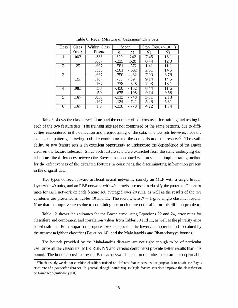
artificial data sets with known Bayes errors are used. Then a more complex 6-class radar data set,

also with known error rate, is examined. Subsequently, the combiner-based estimates are applied to

a real-life underwater sonar problem. Finally, we present results from two data sets extracted from

the Proben1 benchmarks [47]. In all the following tables, the plus/minus figures are provided to

derive various confidence intervals (e.g., we provide σ√N

, where σ is the standard deviation, and N

is the number of elements in the average). For example, for a confidence interval of 95%, one needs

to multiply the plus/minus figures by t .025N−1).

5.1 Artificial Data

In this section, we apply the method to two artificial problems with known Bayes error rates. Both

these problems are taken from Fukunaga [25], and are 8-dimensional, 2-class problems, where each

5This situation typically indicates an outlier or a mislabeled pattern.6In rare occasions, combiners based on posteriors (e.g., averaging) can correct these errors by having a single correct

decision override the erroneous decisions of a larger number of classifiers.

12

class has a Gaussian distribution with equal priors. For each problem, the class means and the

diagonal elements of the covariance matrices (off-diagonal elements are zero) are given in Table 2.

From these specifications, we first generated 1000 training examples and 1000 test examples. Then

we generated a second set of training/test sets with 100 patterns in each. The goal of the second step

in this experiment is to insure that the method works with small sample sizes. The Bayes error rate

for both these problems (10% for DATA1 and 1.9% for DATA2) is given in Fukunaga [25].

Table 2: Artificial Data Sets.

Data Set i (dimension)Characteristics 1 2 3 4 5 6 7 8

µ1 0 0 0 0 0 0 0 0DATA1 σ1 1 1 1 1 1 1 1 1

µ2 2.56 0 0 0 0 0 0 0σ2 1 1 1 1 1 1 1 1µ1 0 0 0 0 0 0 0 0

DATA2 σ1 1 1 1 1 1 1 1 1µ2 3.86 3.10 0.84 0.84 1.64 1.08 0.26 0.01σ2 8.41 12.06 0.12 0.22 1.49 1.77 0.35 2.73

It is a well-known result that the outputs of certain properly trained feed-forward artificial

neural networks approximate the class posteriors [6, 48, 50]. Therefore, these networks provide a

suitable choice for the multiple classifier combining scheme discussed in Section 3.1. Two different

types of networks were selected for this application. The first is a multi-layered perceptron (MLP),

and the second is a radial basis function (RBF) network. A detailed account on how to select, design

and train these networks is available in Haykin [36].

The single hidden layered MLP used for DATA1 had 5 units, and the RBF network had 5

kernels, or centroids7 . For DATA2 the number of hidden units and the number of kernels were

increased to 12. For the case with 100 training/test samples, 5 different training/test sets were

generated and 20 runs were performed on each set. The reported results are the averages over

both the different samples and different runs. Note that more elaborate cross-validation is really

not needed for this simple problem. For the case with 1000 training/test samples, the variability

between selecting different training sets was minimal. For that reason we report the results of 20

runs on one typical set of 1000 training/test samples.

Tables 3 and 4 provide the correlation factors and combining results, for DATA1 and DATA2

respectively. Notice that for the 1000 sample case, the MLP combining results for DATA1 fail

to show any improvements over individual classifiers (row with N = 1). This is caused by the

simplicity of the problem and the lack of variability among different MLPs. The similarity between

MLPs can be confirmed by the high correlation among them as shown in Tables 3 and 4. The RBF

networks suffer less from the high correlations, since variations between kernel locations introduces

7The network sizes were established experimentally.

13

differences that cannot be introduced in an MLP. Consequently, combining RBFs does provide

moderate improvements over single RBF results. In general, using a smaller sample size reduces

the correlation among the individual classifiers, at the expense of classification performance. The

lone exception is the mutual information based estimate for MLPs where a reduction in sample size

actually increases the correlation.

Table 3: Combining Results and Correlations for Artificial Data 1.

Type of Number of 1000 samples 100 samplesClassifier Classifiers Error Rate Error Rate

(in %) δMI δPOS (in %) δMI δPOS

1 10.52 ± 0.04 13.02 ± 0.17MLP 3 10.55 ± 0.02 .86 13.03 ± 0.17 .89

5 10.54 ± 0.02 .87 .99 12.90 ± 0.17 .89 .967 10.53 ± 0.02 .87 12.88 ± 0.15 .901 10.39 ± 0.18 12.54 ± 0.57

RBF 3 10.06 ± 0.09 .60 12.19 ± 0.43 .505 10.13 ± 0.06 .61 .82 11.98 ± 0.33 .52 .677 10.16 ± 0.06 .62 11.90 ± 0.29 .533 10.32 ± 0.06 .61 11.48 ± 0.33 .51

MLP/RBF 5 10.34 ± 0.04 .63 .62 11.51 ± 0.28 .52 -.017 10.33 ± 0.03 .64 11.33 ± 0.27 .52

Table 4: Combining Results and Correlations for Artificial Data 2.

Type of Number of 1000 samples 100 samplesClassifier Classifiers Error Rate Error Rate

(in %) δMI δPOS (in %) δMI δPOS

1 3.22 ± 0.09 5.63 ± 0.13MLP 3 3.10 ± 0.06 .82 5.62 ± 0.11 .94

5 3.11 ± 0.05 .83 .91 5.59 ± 0.09 .94 .997 3.12 ± 0.05 .83 5.58 ± 0.11 .951 3.49 ± 0.06 6.00 ± 0.66

RBF 3 3.33 ± 0.04 .58 4.42 ± 0.47 .435 3.36 ± 0.03 .60 .71 3.78 ± 0.35 .45 .537 3.31 ± 0.02 .61 3.51 ± 0.31 .463 2.77 ± 0.05 .62 4.24 ± 0.13 .45

MLP/RBF 5 2.67 ± 0.05 .63 .35 4.31 ± 0.12 .47 -.277 2.65 ± 0.04 .63 4.35 ± 0.11 .48

Table 5 shows the different estimates for the Bayes error. For each data set, the Bayes error

is estimated through the combining results, using Tables 3, 4, and Equations 22 and 24. Each row

of Tables 3 and 4 provide an estimate for the Bayes error. These values are averaged to yield the

results that are reported. When the correlation among classifiers is close to one, the Bayes estimate

becomes unreliable because the denominator in Equations 22 and 24 is near zero. In such cases, it

is not advisable to use the classifiers with high correlation in the Bayes estimate equation. The EPOS

error estimates reported in this article are based on classifiers whose correlations (δPOS) were less

14

Table 5: Bayes Error Estimates for Artificial Data (given in %).

DATA 1 DATA 2Actual Bayes Error 10.00 1.90Mahalanobis Bound Ebayes ≤ 18.95 Ebayes ≤ 14.13

(True mean and covariance) (∆ = 6.55) (∆ = 10.16)Bhattacharyya bounds 5.12 ≤ Ebayes ≤ 22.04 0.23 ≤ Ebayes ≤ 4.74

(True mean and covariance) (ρ = 0.82) (ρ = 2.36)EPOS 9.24 ± .33 2.15 ± .17

(1000 samples)EMI 9.96 ± .12 2.05 ± .24

(1000 samples)EPLU 9.29 ± .11 2.59 ± .12

(1000 samples)Nearest Neighbor Bounds 8.73 ≤ Ebayes ≤ 15.94 2.15 ≤ Ebayes ≤ 4.20

(1000 samples)EPOS 10.70 ± .21 2.36 ± .25

(100 samples)EMI 10.56 ± .36 2.53 ± .52

(100 samples)EPLU 9.47 ± .22 2.70 ± .17

(100 samples)Nearest Neighbor Bounds 8.62 ≤ Ebayes ≤ 15.76 2.43 ≤ Ebayes ≤ 4.75

(100 samples)

than an experimentally selected threshold8 . For example, based on the correlations in Table 3, for

DATA1 with 1000 samples, only RBF networks and RBF/MLP hybrids were used in determining

the Bayes estimate, whereas for DATA1 with 100 samples, all available classifiers (MLPs, RBFs

and MLP/RBF hybrids) were used.

Studying Tables 3, 4 and 5, leads us to conclude that the performance of the base classifiers has

little impact on the final estimate of the Bayes error. For example, for DATA1, when the individual

classifiers were trained and tested on 1000 patterns, they performed well, coming close in perfor-

mance to the true Bayes error rate. In those cases, combining provided limited improvements, if

at all. For individual classifiers trained and tested on only 100 samples, on the other hand, neither

MLPs nor RBF networks provided satisfactory results. Combining provided moderate improve-

ments in some, but not all cases (note that combining multiple MLPs still yielded poor results). Yet,

the Bayes error estimates were still accurate and close to both the true rate and the rate obtained

with 1000 samples. This confirms that the method is not sensitive to the actual performance of its

classifiers, but to the interaction between the individual classifier performance, combiner perfor-

mance and the correlation among the classifiers. The Bayes error estimate only becomes unreliable

when the classifier errors start to become exceedingly large, a case where the assumption that the

classifiers approximate the class posterior breaks down. We observe this phenomenon for DATA2

with the small sample size where 100 samples is not enough to learn the complex 8 dimensional

8For this study, only classifiers with correlations less than or equal to .97 were used.

15

Gaussian structure.

For the Mahalanobis and Bhattacharyya distances, the bounds were based on the true mean and

covariance matrices. (Using sample means and covariances would have further weakened the re-

sults.) Notice that although the Bhattacharyya bound is expected to be tighter than the Mahalanobis

bound, this is not so for DATA1. The reason for this discrepancy is twofold: first, the Mahalanobis

distance provides tighter bounds as the error becomes larger [14]; second, two terms contribute to

the distance of Equation 7, one for the difference of the means and one for the difference of the

covariances. In the case where the covariances are identical, the second term is zero, leading to a

small Bhattacharyya distance, which in turn leads to a loose bound on the error. DATA1, by virtue

of having a large Bayes error due exclusively to the separation of the class means, represents a case

where the Bhattacharyya bound fails to improve on the Mahalanobis bound. For DATA2, the Bhat-

tacharyya distance provides bounds that are more useful, and the upper bound in particular is very

similar to the upper bound provide by the NN method. For both DATA1 and DATA2, the Bayes error

rate estimates obtained through the classifier combining method introduced in this article provide

estimates closer to the true error than any of the traditional methods. This is particularly remark-

able since both experiments are biased towards the classical techniques because they have Gaussian

distributions. Furthermore, both for DATA1 and DATA2 and for both sample sizes, the MI-based

method provides the most accurate Bayes error estimates among the combiner-based methods.

5.2 Radar Data

The radar data set, provided by Pat Shoemaker [56], represents estimated probability densities for a

six-class problem based on two particular characteristics of radar emissions. The data set is visual-

ized in Figure 1, and summarized in Table 6, where we provide the means and diagonal covariances

of the two-dimensional Gaussians that constitute each of the six classes. The within class priors

determine the preponderance of each particular Gaussian within that class, whereas the class priors

determine the relative frequency of that particular class.

Five of the six classes consist of mixtures of Gaussians with diagonal variances, while the sixth

is a single Gaussian. The data set is normalized to lie within the square −1 ≤ x1,x2 ≤ 1. Thus this

is a fairly complex data set, but its optimal (Bayes) error rate is known to be 3.7% [56]. In previous

work on this data set, based on training/test sizes of 600/1200, rates between 84.4% and 95.5% were

achieved by 6 different network types (MLP, RBF, etc), each with 4 different settings of network

sizes [4].

In the experiments reported here, we used 600 training samples, and 1200 test samples. The

MLPs had a single hidden layer that consists of 10 units, and were trained for 80 epochs, determined

by a validation set. The RBF networks had 12 kernels, and each class had at least one kernel initially

assigned to it. The RBF networks where both the kernel sizes and location were modified during

16

−1

−0.5

0

0.5

1

−1

−0.5

0

0.5

1

0

2

4

6

8

x1

x2

f(x)

Figure 1: Class densities for the radar data set.

training were trained for 60 epochs.

Table 7 provides the classification and combining results, along with the correlation estimates.

The posterior-based correlation for combining multiple MLPs is once again very high, indicating

both that the combining should provide minimal gains and that the Bayes error estimates based on

this value (EPOS) are not to be trusted9 . Table 8 provides the Bayes errors for the different methods.

Once again, the MI-based ensemble method provides the most accurate Bayes error estimate.

5.3 Underwater Sonar Data

The previous section dealt with obtaining the Bayes error for artificial problems with known Bayes

error. In this section, we apply the method to a difficult underwater sonar problem. From the

original sonar signals of four different underwater sources, two qualitatively different feature sets

are extracted [33]. The first one (FS1), a 25-dimensional set, consists of Gabor wavelet coefficients,

temporal descriptors and spectral measurements. The second feature set (FS2), a 24-dimensional

set, consists of reflection coefficients based on both short and long time windows, and temporal

descriptors.

9We follow the same criterion as in the previous section and disregard classifiers for which δPOS ≥ .97. In fact this

“worsens” EPOS, as including the MLP results (which are artificially low due to the high correlation) lowers the estimate

to EPOS = 3.6%.

17

Table 6: Radar (Mixture of Gaussians) Data Sets.

Class Class Within Class Mean Stan. Dev. (×10−3)Priors Priors x1 x2 σ1 σ2

1 .083 .333 .600 .242 7.45 13.1.667 -.225 .528 8.44 12.0

2 .25 .667 -.581 -.572 1.41 11.1.333 -.581 -.682 2.81 14.5

3 .667 -.750 -.462 7.03 6.78.25 .167 .788 -.594 9.14 14.5

.167 -.338 -.528 7.03 13.14 .083 .50 -.450 -.132 8.44 11.6

.50 -.675 -.198 9.14 9.685 .167 .836 -.113 -.748 3.51 2.13

.167 -.124 -.741 5.48 5.816 .167 1.0 -.338 -.770 4.22 1.74

Table 9 shows the class descriptions and the number of patterns used for training and testing in

each of the two feature sets. The training sets are not comprised of the same patterns, due to diffi-

culties encountered in the collection and preprocessing of the data. The test sets however, have the

exact same patterns, allowing both the combining and the comparison of the results10 . The avail-

ability of two feature sets is an excellent opportunity to underscore the dependence of the Bayes

error on the feature selection. Since both feature sets were extracted from the same underlying dis-

tributions, the differences between the Bayes errors obtained will provide an implicit rating method

for the effectiveness of the extracted features in conserving the discriminating information present

in the original data.

Two types of feed-forward artificial neural networks, namely an MLP with a single hidden

layer with 40 units, and an RBF network with 40 kernels, are used to classify the patterns. The error

rates for each network on each feature set, averaged over 20 runs, as well as the results of the ave

combiner are presented in Tables 10 and 11. The rows where N = 1 give single classifier results.

Note that the improvements due to combining are much more noticeable for this difficult problem.

Table 12 shows the estimates for the Bayes error using Equations 22 and 24, error rates for

classifiers and combiners, and correlation values from Tables 10 and 11, as well as the plurality error

based estimate. For comparison purposes, we also provide the lower and upper bounds obtained by

the nearest neighbor classifier (Equation 14), and the Mahalanobis and Bhattacharyya bounds.

The bounds provided by the Mahalanobis distance are not tight enough to be of particular

use, since all the classifiers (MLP, RBF, NN and various combiners) provide better results than this

bound. The bounds provided by the Bhattacharyya distance on the other hand are not dependable

10In this study we do not combine classifiers trained on different feature sets, as our purpose is to obtain the Bayes

error rate of a particular data set. In general, though, combining multiple feature sets does improve the classification

performance significantly [60].

18

Table 7: Combining Results for the Radar Data.

Type of Number of Error RateClassifier Classifiers (in %) δMI δPOS

1 5.95 ± 0.053 5.86 ± 0.04 .91

MLP 5 5.79 ± 0.03 .92 .977 5.80 ± 0.03 .92

11 5.76 ± 0.02 .9215 5.77 ± 0.02 .921 5.42 ± 0.083 5.17 ± 0.02 .68

RBF 5 5.14 ± 0.02 .69 .787 5.14 ± 0.02 .70

11 5.11 ± 0.01 .7015 5.12 ± 0.01 .703 5.31 ± 0.03 .815 5.34 ± 0.02 .82

MLP/RBF 7 5.38 ± 0.02 .82 .6411 5.44 ± 0.02 .8215 5.42 ± 0.02 .82

Table 8: Bayes Error Estimates for Radar Data (given in %).

Actual Bayes Error 3.70EPOS 4.23 ± .14EMI 3.86 ± .13

EPLU 4.72 ± .06Nearest Neighbor Bounds 3.08 ≤ Ebayes ≤ 6.08

due to the assumptions made on the distributions. Equation 7 is derived for Gaussian classes, and

can lead to significant errors when the class distributions are not Gaussian. Furthermore, since

Equations 5 and 8 provide bounds for the 2-class case, and need to be extended to the 4-class case

through the repeated application of Equation 11, the errors are compounded. Therefore, in this case

only bounds provided by the nearest neighbor method can be reliably compared to the combiner-

based estimates.

5.4 Proben1/UCI Benchmarks

In this section we apply the combiner based Bayes error estimation method to selected data sets

from the Proben1 benchmark set11 [47]. The data sets that were included in this study are the

GLASS1, and GENE1 sets, and the name and number combinations correspond to a specific train-

ing/validation/test set split consistent with the Proben1 benchmarks. Note that these two data sets

11Available at URL ftp://ftp.ira.uka.de/pub/papers/techreports/1994/1994-21.ps.Z.

19

Table 9: Description of Data for Underwater Sonar Data

Class Feature Set 1 Feature Set 2Description Training Testing Training Testing

Porpoise Sound 116 284 142 284Ice 116 175 175 175Whale Sound 1 116 129 129 129Whale Sound 2 148 235 118 235Total 496 823 564 823

Table 10: Combining Results for the Sonar Data (FS1).

Type of Number of Error RateClassifier Classifiers (in %) δMI δPOS

1 7.47 ± 0.103 7.19 ± 0.06 .78

MLP 5 7.13 ± 0.06 .79 .887 7.11 ± 0.05 .80

11 7.11 ± 0.04 .801 6.79 ± 0.093 6.15 ± 0.07 57

RBF 5 6.05 ± 0.04 60 .707 5.97 ± 0.05 60

11 5.86 ± 0.04 613 6.11 ± 0.08 60

MLP/RBF 5 6.11 ± 0.07 62 .357 6.08 ± 0.07 63

11 6.07 ± 0.08 63

are also available from the UCI machine learning repository12 [7]. However, the training/test sets

used in this study are from with the Proben1 splits and therefore the results presented here cannot

be meaningfully compared to results from different training/test set splits obtained from the UCI

repository.

GENE1 is based on intron/exon boundary detection, or the detection of splice junctions in

DNA sequences [42, 57]. 120 inputs are used to determine whether a DNA section is a donor, an

acceptor or neither. There are 3175 examples, of which 1588 are used for training. The GLASS1

data set is based on the chemical analysis of glass splinters. The 9 inputs are used to classify 6

different types of glass. There are 214 examples in this set, and 107 of them are used for training.

Table 13 contains the combining results and the two correlation estimates for the GLASS1

data, and Table 14 presents the combining results for the GENE1 data, along with the correlation

estimates. Because for GENE1 the correlations among multiple RBF networks is .98, care must be

taken in estimating the Bayes error. More precisely, even moderate improvements in classification

12URL: http://www.ics.uci.edu/∼mlearn/MLRepository.html

20

Table 11: Combining Results for the Sonar Data (FS2).

Type of Number of Error RateClassifier Classifiers (in %) δMI δPOS

1 9.95 ± 0.173 9.32 ± 0.08 .68

MLP 5 9.20 ± 0.07 .70 .767 9.07 ± 0.08 .71

11 9.03 ± 0.06 .721 10.94 ± 0.213 10.55 ± 0.10 .52

RBF 5 10.43 ± 0.07 .54 .727 10.44 ± 0.07 .55

11 10.38 ± 0.04 .563 8.46 ± 0.13 .52

MLP/RBF 5 8.17 ± 0.09 .55 .207 8.14 ± 0.06 .55

11 8.04 ± 0.04 .56

Table 12: Bayes Error Estimates for Sonar Data (given in %).

DATA 1 DATA 2EPOS 4.20 ± .18 7.21 ± .31EMI 4.55 ± .19 6.83 ± .56

EPLU 5.37 ± .22 7.49 ± .35Nearest Neighbor Bounds 3.27 ≤ Ebayes ≤ 6.40 6.88 ≤ Ebayes ≤ 13.12

Mahalanobis Bound ≤ 14.61 ≤ 19.53Bhattacharyya bound ≤ 0.20 ≤ 1.10

rates with high correlation imply zero or near zero Bayes error rates. Therefore, we estimate the

Bayes error rate through combining MLPs and MLP/RBF hybrids only, as discussed in Section 5.1.

Table 15 presents the Bayes error estimates for both GLASS1 and GENE1 problems. We have

also included the nearest neighbor bounds for these two data sets based on Equation 14, denoted by

Ennbayes in the last column. Note that for the GENE1 problem the nearest neighbor method fails to pro-

vide accurate bounds (e.g., all the classifiers exceed the so-called “bound” provided by the nearest

neighbor). The failure of the nearest neighbor in this case is mainly due to the high-dimensionality

of the problem, where proximity in Euclidean sense is not necessarily a good measure for class be-

longings. For the GLASS1 data set the three combining based estimates provide particularly close

estimates, while for GENE1, the estimates are within 10% of each other.

6 CONCLUSION

Ensembles have become a popular way of tackling difficult classification problems. The signifi-

cance of this paper lies in showing that certain ensembles have a very beneficial side result: they

21

Table 13: Combining Results for the GLASS1 Data.

Type of Number of Error RateClassifier Classifiers (in %) δMI δPOS

1 32.26 ± 0.133 32.08 ± 0.00 .84

MLP 5 32.08 ± 0.00 .85 0.927 32.08 ± 0.00 .85

11 32.08 ± 0.00 .861 31.79 ± 0.783 29.81 ± 0.51 .50

RBF 5 29.25 ± 0.41 .52 0.687 29.06 ± 0.34 .53

11 28.67 ± 0.29 .533 30.66 ± 0.12 .50

MLP/RBF 5 32.36 ± 0.18 .50 0.087 32.45 ± 0.21 .50

11 32.45 ± 0.17 .50

Table 14: Combining Results for the GENE1 Data.

Type of Number of Error RateClassifier Classifiers (in %) δMI δPOS

1 13.47 ± 0.103 12.30 ± 0.09 .57

MLP 5 12.23 ± 0.09 .60 0.737 12.08 ± 0.05 .61

11 12.13 ± 0.06 .621 14.62 ± 0.093 14.48 ± 0.08 .79

RBF 5 14.35 ± 0.08 .80 0.987 14.33 ± 0.07 .80

11 14.28 ± 0.07 .813 12.43 ± 0.11 .56

MLP/RBF 5 12.28 ± 0.09 .56 .307 12.17 ± 0.08 .59

11 12.21 ± 0.06 .60

22

Table 15: Bayes Error Estimates for Proben1 Data (given in %).

Glass1 Gene 1EPOS 27.59 ± 1.36 9.19 ± .54EMI 28.75 ± .94 10.39 ± .47

EPLU 27.57 ± .96 9.94 ± .23Nearest Neighbor Bounds 21.69 ≤ Ebayes ≤ 37.74 16.72 ≤ Ebayes ≤ 29.25

provide a mechanism for estimating the Bayes error with little extra computational effort. The first

two techniques presented for obtaining this estimate are based on linear combining theory, and ex-

ploit the ability of certain well-trained neural networks or other universal approximation structures

to directly estimate the posterior probabilities. Experimental results show that this error estimate

compares very favorably with classical estimation methods. Both these techniques are consistent,

and convergence rates can be derived (at least for broad classes of functions) from the behavior of

the constituent classifiers, using well known results on convergence of MLPs [2] and RBFs [44].

The third technique is a heuristic “plurality error” for classifiers trained on specific data sam-

ples. This method’s power lies in its generality, as it applies to any type of base classifier. It is

tailored to determining the best accuracy achievable given a specific data set, and not for estimating

Bayes rate.

For the first two Bayes estimation methods introduced in this article, the estimation of the

correlation (in the deviations of the estimated posterior probabilities from the true values) plays

a crucial role in the accuracy of the Bayes error. It is clear from Equations 20 that when this

correlation is close to 1, the Bayes rate estimation is very sensitive to errors in estimating this

correlation. However, this typically happens only for simple problems, where there is little need for

using an ensemble in the first place. For the difficult real-data based problems, correlation values are

much lower, as evidenced by the experimental results. Moreover, several researchers have shown the

desirability of reducing correlations among classifiers in an ensemble and have proposed methods

to achieve this task [40, 43, 49, 60, 54]. Thus we expect our technique to provide even better results

when applied to ensembles that employ any of these decorrelation methods first.

Further investigation of the power of the proposed methods can be carried out by experimenting

over a larger number of data-sets with known Bayes error rates. As is widely recognized in both

pattern recognition and the theory of function approximation, no method is expected to work best

for all distributions or functions [65, 66], and one can typically come up with pathological examples

to foil any method [15]. Our empirical studies indicate that the proposed methods are indeed quite

versatile, but one can further explore the scope/limitations of these methods through continued

experimentation.

Acknowledgments: The authors would like to thank Kurt D. Bollacker and Rasmus Pedersen for

23

insightful comments. This research was supported in part by NSF grant ECS 9307632, and from a

research gift from Intel Corp.

References

[1] K. M. Ali and M. J. Pazzani. On the link between error correlation and error reduction in

decision tree ensembles. Technical Report 95-38, Department of Information and Computer

Science, University of California, Irvine, 1995.

[2] A. R. Barron. Universal approximation bounds for superpositions of a sigmoidal function

theory. IEEE Transactions on Information Theory, 39(3):930–945, May 1993.

[3] R. Battiti. Using mutual information for selecting features in supervised neural net learning.

IEEE Transactions on Neural Networks, 5:4:537–550, July 1994.

[4] S. Beck and J. Ghosh. Noise sensitivity of static neural classifiers. In SPIE Conf. on Applica-

tions of Artificial Neural Networks SPIE Proc. Vol. 1709, pages 770–779, Orlando, Fl., April

1992.

[5] J.A. Benediktsson and J.R. Sveinsson. Consensus based classification of multisource remote

sensing data. In J. Kittler and F. Roli, editors, Proceedings of the First International Workshop

on Multiple Classifier Systems, pages 280–289. Springer, Berlin, 2000.

[6] C. M. Bishop. Neural Networks for Pattern Recognition. Oxford University Press, New York,

1995.

[7] C. Blake, E. Keogh, and C.J. Merz. UCI repository of machine learning databases, 1998.

(URL: http://www.ics.uci.edu/∼mlearn/MLRepository.html).

[8] K. D. Bollacker and J. Ghosh. Linear feature extractors based on mutual information. In

Proceedings of the 13th International Conference on Pattern Recognition, pages pp. IV:720–

724, 1996.

[9] L. Breiman. Bagging predictors. Machine Learning, 24(2):123–140, 1996.

[10] L. J. Buturovic. Improving k-nearest neighbor density and error estimates. Pattern Recogni-

tion, 26(4):611–616, 1993.

[11] D. Cohn and R. Atlas, L. Ladner. Improving generalization with active learning. Machine

Learning, 15(2):201–221, 1994.

[12] T. M. Cover and P. E. Hart. Nearest neighbor pattern classification. IEEE Transactions on

Information Theory, 13:21–27, 1967.

24

[13] T. M. Cover and J. A. Thomas. Elements of Information Theory. Wiley, 1991.

[14] P.A. Devijver and J. Kittler. Pattern Recognition: A Statistical Approach. Prentice-Hall, 1982.

[15] L. Devroye, L. Gyorfi, and G. Lugosi. A Probabilistic Theory of Pattern Recognition. Springer

Verlag, Berlin, 1996.

[16] T.G. Dietterich. Ensemble methods in machine learning. In J. Kittler and F. Roli, editors,

Proceedings of the First International Workshop on Multiple Classifier Systems, pages 1–15.

Springer, Berlin, 2000.

[17] A. Djouadi, O. Snorrason, and F. D. Garber. The quality of training-sample estimates of the

Battacharyya coefficient. IEEE Transactions on Pattern Analysis and Machine Intelligence,

12(1):92–97, January 1990.

[18] P. Domingos. Bayesian averaging of classifiers and the overfitting problem. In Proceedings of

the Seventeeth International Conference on Machine Learning, pages 223–230, 2000.

[19] H. Drucker, C. Cortes, L. D. Jackel, Y. LeCun, and V. Vapnik. Boosting and other ensemble

methods. Neural Computation, 6(6):1289–1301, 1994.

[20] R. O. Duda, P. E. Hart, and D. G. Stork. Pattern Classification. Wiley, New York, NY, second

edition, 2001.

[21] R.P.W. Duin and D.M.J. Tax. Experiments with classifier combining rules. In J. Kittler and

F. Roli, editors, Proceedings of the First International Workshop on Multiple Classifier Sys-

tems, pages 16–29. Springer, Berlin, 2000.

[22] A. M. Fraser and H. L. Swinney. Independent coordinates for strange attractors from mutual

information. Physical Review A, 33:1134–1140, 2 1986.

[23] Y. Freund and R. Schapire. Experiments with a new boosting algorithm. In Proceedings

of the Thirteenth International Conference on Machine Learning, pages 148–156. Morgan

Kaufmann, 1996.

[24] K. Fukunaga. The estimation of the Bayes error by the k-nearest neighbor approach. In L. N.

Kanal and A. Rosenfeld, editors, Progress in Pattern Recognition 2, pages 169–187. North-

Holland, Amsterdam, 1985.

[25] K. Fukunaga. Introduction to Statistical Pattern Recognition. Academic Press, second edition,

1990.

[26] K. Fukunaga and D. Hummels. Bayes error estimation using Parzen and k-NN procedures.

IEEE Transactions on Pattern Analysis and Machine Intelligence, 9:634–643, 1987.

25

[27] K. Fukunaga and D. Hummels. Bias of the nearest neighbor error estimate. IEEE Transactions

on Pattern Analysis and Machine Intelligence, 9(1):103–112, 1987.

[28] F.D. Garber and A. Djouadi. Bounds on the Bayes classification error based on pairwise risk

functions. IEEE Transactions on Pattern Analysis and Machine Intelligence, 10(3):281–288,

1988.

[29] S. Geman, E. Bienenstock, and R. Doursat. Neural networks and the bias/variance dilemma.

Neural Computation, 4(1):1–58, 1992.

[30] J. Ghosh. Multiclassifier systems: Back to the future. In F. Roli and J. Kittler, editors, Multiple

Classifier Systems, pages invited paper, 1–15. LNCS Vol. 2364, Springer, 2002.

[31] J. Ghosh, L. Deuser, and S. Beck. A neural network based hybrid system for detection, char-

acterization and classification of short-duration oceanic signals. IEEE Journal of Ocean Engi-

neering, 17(4):351–363, October 1992.

[32] J. Ghosh and K. Tumer. Structural adaptation and generalization in supervised feedforward

networks. Journal of Artificial Neural Networks, 1(4):431–458, 1994.

[33] J. Ghosh, K. Tumer, S. Beck, and L. Deuser. Integration of neural classifiers for passive sonar

signals. In C.T. Leondes, editor, Control and Dynamic Systems—Advances in Theory and

Applications, volume 77, pages 301–338. Academic Press, 1996.

[34] G. Giacinto and F. Roli. Dynamic classifier selection. In J. Kittler and F. Roli, editors, Pro-

ceedings of the First International Workshop on Multiple Classifier Systems, pages 177–189.

Springer, Berlin, 2000.

[35] S. Hashem. Optimal Linear Combinations of Neural Networks. PhD thesis, Purdue University,

December 1993.

[36] S. Haykin. Neural Networks: A Comprehensive Foundation. Macmillan, New York, 1994.

[37] Robert Jacobs. Method for combining experts’ probability assessments. Neural Computation,

7(5):867–888, 1995.

[38] H. Kargupta and P. Chan, editors. Advances in Distributed and Parallel Knowledge Discovery.

AAAI/MIT Press, Cambridge, MA, 2000.

[39] J. Kittler and F. Roli, editors. Multiple Classifier Systems: Proceedings of the First Interna-

tional Workshop, Cagliari, Italy, June 2000. Springer, 2000.

[40] A. Krogh and J. Vedelsby. Neural network ensembles, cross validation and active learning.

In G. Tesauro, D. S. Touretzky, and T. K. Leen, editors, Advances in Neural Information

Processing Systems-7, pages 231–238. M.I.T. Press, 1995.

26

[41] D. Lowe and A. R. Webb. Optimized feature extraction and the Bayes decision in feed-forward

classifier networks. IEEE Trans. PAMI, 13:355–364, April 1991.

[42] M. O. Noordewier, G. G. Towell, and J. W. Shavlik. Training knowledge-based neural net-

works to recognize genes in DNA sequences. In R.P. Lippmann, J.E. Moody, and D.S. Touret-

zky, editors, Advances in Neural Information Processing Systems-3, pages 530–536. Morgan

Kaufmann, 1991.

[43] D. W. Opitz and J. W. Shavlik. Generating accurate and diverse members of a neural-network

ensemble. In D. S. Touretzky, M. C. Mozer, and M. E. Hasselmo, editors, Advances in Neural

Information Processing Systems-8, pages 535–541. M.I.T. Press, 1996.

[44] J. Park and I.W. Sandberg. Universal approximation and radial basis function networks. Neural

Computation, 5:305–316, 1993.

[45] M. P. Perrone. Improving Regression Estimation: Averaging Methods for Variance Reduction

with Extensions to General Convex Measure Optimization. PhD thesis, Brown University,

May 1993.

[46] M.P. Perrone and L. N. Cooper. When networks disagree: Ensemble methods for hybrid neural

networks. In R. J. Mammone, editor, Neural Networks for Speech and Image Processing,

chapter 10. Chapmann-Hall, 1993.

[47] Lutz Prechelt. PROBEN1 — A set of benchmarks and benchmarking rules for neural net-

work training algorithms. Technical Report 21/94, Fakultat fur Informatik, Universitat Karl-

sruhe, D-76128 Karlsruhe, Germany, September 1994. Anonymous FTP: /pub/papers/tech-

reports/1994/1994-21.ps.Z on ftp.ira.uka.de.

[48] M.D. Richard and R.P. Lippmann. Neural network classifiers estimate Bayesian a posteriori

probabilities. Neural Computation, 3(4):461–483, 1991.

[49] B. Rosen. Ensemble learning using decorrelated neural networks. Connection Science, Special

Issue on Combining Artificial Neural Networks: Ensemble Approaches, 8(3 & 4):373–384,

1996.

[50] D. W. Ruck, S. K. Rogers, M. E. Kabrisky, M. E. Oxley, and B. W. Suter. The multilayer

Perceptron as an approximation to a Bayes optimal discriminant function. IEEE Transactions

on Neural Networks, 1(4):296–298, 1990.

[51] A. Sharkey. Combining Artificial Neural Nets. Springer-Verlag, 1999.

[52] A. J. C. Sharkey. On combining artificial neural nets. Connection Science, Special Issue on

Combining Artificial Neural Networks: Ensemble Approaches, 8(3 & 4):299–314, 1996.

27

[53] A. J. C. Sharkey, N. E. Sharkey, and G.O. Chandroth. Neural nets and diversity. In Proceedings

of the 14th International Conference on Computer Safety, Reliability and Security, pages 375–

389, Belgirate, Italy, 1995.

[54] A.J.C. Sharkey and N.E. Sharkey. Combining diverse neural nets. The Knowledge Engineering

Review, 12(3):231–247, 1997.

[55] A.J.C Sharkey, N.E. Sharkey, U Gerecke, and G.O. Chandroth. The ‘test and select’ approach

to ensemble combination. In J. Kittler and F. Roli, editors, Proceedings of the First Interna-

tional Workshop on Multiple Classifier Systems, pages 30–44. Springer, Berlin, 2000.

[56] P.A. Shoemaker, M.J. Carlin, R.L. Shimabukuro, and C.E. Priebe. Least squares learning and

approximation of posterior probabilities on classification problems by neural network models.

In Proc. 2nd Workshop on Neural Networks, WNN-AIND91,Auburn, pages 187–196, February

1991.

[57] G. G. Towell and J. W. Shavlik. Interpretation of artificial neural networks: Mapping

knowledge-based neural networks into rules. In J.E. Moody, S.J. Hanson, and R.P. Lippmann,

editors, Advances in Neural Information Processing Systems-4, pages 977–984. Morgan Kauf-

mann, 1992.

[58] K. Tumer, K. D. Bollacker, and J. Ghosh. A mutual information based ensemble method to es-

timate the Bayes error. In Intelligent Engineering Systems through Artificial Neural Networks,

C. Dagli et al., Eds., volume 8, pages 17–22. ASME Press, 1998.

[59] K. Tumer and J. Ghosh. Analysis of decision boundaries in linearly combined neural classi-

fiers. Pattern Recognition, 29(2):341–348, February 1996.

[60] K. Tumer and J. Ghosh. Error correlation and error reduction in ensemble classifiers. Connec-

tion Science, 8(3 & 4):385–404, 1996.

[61] K. Tumer and J. Ghosh. Linear and order statistics combiners for pattern classification. In

A. J. C. Sharkey, editor, Combining Artificial Neural Nets: Ensemble and Modular Multi-Net

Systems, pages 127–162. Springer-Verlag, London, 1999.

[62] K. Tumer and J. Ghosh. Robust combining of disparate classifiers through order statistics.

Pattern Analysis and Applications, 5(2):189–200, 2002.

[63] K Tumer and N. C. Oza. Input decimnated ensembles. Pattern Analysis and Applications,

2003. to appear.

[64] K. Tumer, N. Ramanujam, R. Richards-Kortum, and J. Ghosh. Spectroscopic detection of

cervical pre-cancer through radial basis function networks. In M. C. Mozer, M. I. Jordan, and

28

T. Petsche, editors, Advances in Neural Information Processing Systems-9, pages 981–987.

M.I.T. Press, 1997.

[65] D. H. Wolpert. The existence of a priori distinctions between learning algorithms. Neural

Computation, 8:1391–1420, 1996.

[66] D. H. Wolpert. The lack of a priori distinctions between learning algorithms. Neural Compu-

tation, 8:1341–1390, 1996.

[67] T. Y. Young and T. W Calvert. Classification, Estimation and Pattern Recognition. Elsevier,

New York, 1974.

[68] Z. Zheng and G.I. Webb. Stochastic attribute selection committees. In Proceedings of the

Eleventh Australian Joint Conference on Artificial Intelligence (AI’98), pages 321–332, 1998.

29


Recommended