Bayes-optimal Policies for Multiple Comparisons with aKnown Standard

Jing Xie and Peter I. Frazier

Operations Research & Information Engineering, Cornell University

Monday January 7, 2013INFORMS Computing Society Conference

Sante Fe, NM

Supported by AFOSR YIP #FA9550-11-1-0083

What is Multiple Comparisons with a Known Standard?

We have a stochastic simulator.

Given a set of input parameters x , it provides a random sample y(x).

For which inputs x is E [y(x)] > 0?

●

●

● ●

●

●

●

●

●

●

●

●

●

●

●

●

●

●

●

●

●

●

●

●

●

●

● ● ●

●

●

●

●

●●

●

● ●

●

●

● ●

●

●●

● ●

●

●

●

●

●

●

●

●

●

●

● ●

●

y(n)

f(x)

In other words, find the level set of x 7→ E[f (x)].

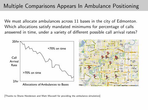
Multiple Comparisons Appears In Ambulance Positioning

We must allocate ambulances across 11 bases in the city of Edmonton.Which allocations satisfy mandated minimums for percentage of callsanswered in time, under a variety of different possible call arrival rates?

Call

Arrival

Rate

Allocations of Ambulances to Bases

>70% on time

<70% on time

2/hr

20/hr

[Thanks to Shane Henderson and Matt Maxwell for providing the ambulance simulation]

We Provide an Optimal Way to Choose Where to Sample

If our simulator is complex and takes a long time to run, the numberof samples we can take is limited.

This makes accurate MCC more difficult.

Where should we place our limited samples to estimate thelevel set as accurately as possible?

Our contribution: We provide an answer to this question withBayes-optimal performance.

Literature Review

Procedures with frequentist indifference-style guarantees on solutionquality: [Paulson, 1962, Kim, 2005, Bechhofer and Turnbull, 1978,Nelson and Goldsman, 2001, Andradottir et al., 2005,Andradottir and Kim, 2010, Batur and Kim, 2010,Healey et al., 2012]

Procedures based on large deviations analysis, which use allocationsthat minimize the rate of decay of the error probability as the samplesize grows to infinity: [Szechtman and Yucesan, 2008,Hunter and Pasupathy, 2010, Hunter and Pasupathy, 2012].

All of this literature is in the frequentist setting. We focus onsampling sequentially in a Bayes-optimal way, and use anon-asymptotic analysis.

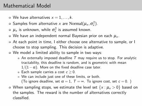
Mathematical Model

We have alternatives x = 1, . . . ,k.

Samples from alternative x are Normal(µx ,σ2x ).

µx is unknown, while σ2x is assumed known.

We have an independent normal Bayesian prior on each µx .

At each point in time, I either choose one alternative to sample, or Ichoose to stop sampling. This decision is adaptive.

We model a limited ability to sample in two ways:An externally imposed deadline T may require us to stop. For analytictractability, this deadline is random, and is geometric with mean1/(1−α). More on the fixed deadline case later.Each sample carries a cost c ≥ 0.We can include just one of these limits, or both.(To ignore deadline, set α = 1, T = ∞. To ignore cost, set c = 0. )

When sampling stops, we estimate the level set {x : µx > 0} based onthe samples. The reward is the number of alternatives correctlyclassified.

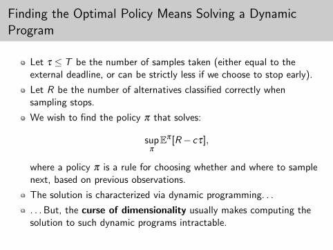
Finding the Optimal Policy Means Solving a DynamicProgram

Let τ ≤ T be the number of samples taken (either equal to theexternal deadline, or can be strictly less if we choose to stop early).

Let R be the number of alternatives classified correctly whensampling stops.

We wish to find the policy π that solves:

supπ

Eπ [R− cτ],

where a policy π is a rule for choosing whether and where to samplenext, based on previous observations.

The solution is characterized via dynamic programming. . .

. . . But, the curse of dimensionality usually makes computing thesolution to such dynamic programs intractable.

We Rewrite the Problem as a Bandit Problem

Let’s analyze the case where we have a geometric external deadline(α < 1), and no sampling costs (c = 0). Then τ = T is optimal, andwe choose π to maximize Eπ [R].

The expected reward is the expected number of alternatives correctlyclassified at the end.

We decompose this expected reward into an infinite sum ofdiscounted expected one-step rewards

Eπ [R] = R0 +Eπ

[∞

∑n=1

αn−1Rn

].

Here,

α is the parameter of the geometric distribution of the deadline.

R0 is the expected reward if we stop after taking no samples.

Rn is the expected one-step improvement, due to sampling, of theprobability of correctly classifying the alternative sampled.

We Can Compute the Optimal Policy

Written in this way, the problem becomesa multi-armed bandit problem.

[Gittins and Jones, 1974] shows theoptimal solution is

arg maxx

νx(Snx),

where Snx is a parameterization of theBayesian posterior on µx .

The Gittins index νx(·) is defined in terms of a single-alternativeversion of the problem

νx(s) = supρ>0

E[∑

ρ

n=1 αn−1Rn|S0x = s,x1 = · · ·= xρ = x]

E[∑

ρ

n=1 αn−1|S0x = s,x1 = · · ·= xρ = x] .

We can compute Gittins indices efficiently because thesingle-alternative problem is much smaller than the full DP.

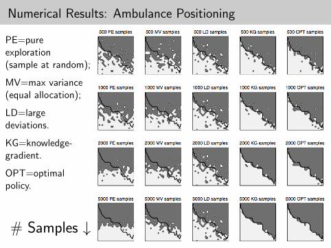
Numerical Results: Ambulance Positioning

PE=pureexploration(sample at random);

MV=max variance(equal allocation);

LD=largedeviations.

KG=knowledge-gradient.

OPT=optimalpolicy.

# Samples ↓

What About Other Ways of Modeling A Limited Ability toSample?

Recall that we were considering the case with α < 1 and c = 0(geometric deadline and no sampling costs).

If α < 1 and c > 0, we can rewrite the problem as a slightly differentbandit problem and also compute the optimal policy.

If α = 1 (no external deadline) and c > 0, then we can decomposeacross alternatives in a different way (not a bandit problem), andagain compute the optimal policy.

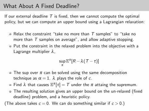
What About A Fixed Deadline?

If our external deadline T is fixed, then we cannot compute the optimalpolicy, but we can compute an upper bound using a Lagrangian relaxation:

Relax the constraint “take no more than T samples” to “take nomore than T samples on average”, and allow adaptive stopping.

Put the constraint in the relaxed problem into the objective with aLagrange multiplier λ ,

supπ

Eπ [R−λ (T − τ)]

The sup over π can be solved using the same decompositiontechnique as α = 1. λ plays the role of c .

Find λ that causes Eπ [τ] = T under the π attaing the supremum.

The resulting solution gives an upper bound on the un-relaxed (fixeddeadline) problem, and a heuristic policy.

(The above takes c = 0. We can do something similar if c > 0.)

Other Generalizations are Possible

Rather Normal(µx ,σ2x ) samples with a normal prior on µx and σ2

xknown, the same method works when the sampling distribution isfrom an exponential family, and we have the conjugate prior.

e.g., normal samples with unknown mean and unknown variance, witha Normal/inverse-gamma prior.e.g., Bernoulli samples with a Beta prior.

Rather than taking our reward to be the number of correctclassifications, we can have more complex functions of the truesampling distribution and the classification decision. Examples:

e.g., Reward of θx when we classify θx as positive, and a reward of 0when we classify θx as negative.e.g., Pay a penalty of a when we incorrectly classify an x with θx < 0,and a penalty of b when we incorrectly classify an x with θx > 0.

Numerical Results: Idealized Test Problems

Here, costs are 0, and we have a geometric external deadline.

Comparison policies: Pure Exploration (PE), Max Variance (MV),Large Deviations (LD), Knowledge Gradient (KG), and Bayes-Optimal(OPT).

Numerical Results: Idealized Test Problems

Here, costs are strictly positive, and there is no external deadline.

Comparison policies: Pure Exploration (PE), Max Variance (MV),Andradottir and Kim (AK), Knowledge Gradient (KG), andBayes-Optimal (OPT).

Conclusion: The Optimal Policy Saves Time

The Multiple Comparisons with a Control problem appears inmany different simulation applications.

We found the optimal method for deciding where to sample.

This allows accurately characterizing level sets more quickly and withfewer simulation samples.

Thank You

Any questions?

References I

Andradottir, S., Goldsman, D., and Kim, S. (2005).Finding the best in the presence of a stochastic constraint.In Simulation Conference, 2005 Proceedings of the Winter, pages7–pp. IEEE.

Andradottir, S. and Kim, S. (2010).Fully sequential procedures for comparing constrained systems viasimulation.Naval Research Logistics (NRL), 57(5):403–421.

Batur, D. and Kim, S. (2010).Finding feasible systems in the presence of constraints on multipleperformance measures.ACM Transactions on Modeling and Computer Simulation(TOMACS), 20(3):13.

References II

Bechhofer, R. and Turnbull, B. (1978).Two (k+1)-decision selection procedures for comparing k normalmeans with a specified standard.Journal of the American Statistical Association, pages 385–392.

Gittins, J. C. and Jones, D. M. (1974).A dynamic allocation index for the sequential design of experiments.In Gani, J., editor, Progress in Statistics, pages 241–266, Amsterdam.North-Holland.

Healey, C., Andradottir, S., and Kim, S. (2012).Selection procedures for simulations with multiple constraints.in review.

References III

Hunter, S. and Pasupathy, R. (2010).Large-deviation sampling laws for constrained simulation optimizationon finite sets.In Simulation Conference (WSC), Proceedings of the 2010 Winter,pages 995–1002. IEEE.

Hunter, S. and Pasupathy, R. (2012).Optimal sampling laws for stochastically constrained simulationoptimization on finite sets.INFORMS Journal on Computing.

Kim, S. (2005).Comparison with a standard via fully sequential procedures.ACM Transactions on Modeling and Computer Simulation(TOMACS), 15(2):155–174.

References IV

Nelson, B. and Goldsman, D. (2001).Comparisons with a standard in simulation experiments.Management Science, 47(3):449–463.

Paulson, E. (1962).A sequential procedure for comparing several experimental categorieswith a standard or control.The Annals of mathematical statistics, pages 438–443.

Szechtman, R. and Yucesan, E. (2008).A new perspective on feasibility determination.In Proceedings of the 40th Conference on Winter Simulation, pages273–280. Winter Simulation Conference.

The Optimal Policy Maximizes Average-Case Accuracy

A policy π is a rule for choosing whether and where to sample next,based on previous observations.

Let τ ≤ T be the number of samples taken (either equal to theexternal deadline, or can be strictly less if we choose to stop early).

Let R be the number of alternatives classified correctly whensampling stops.

Eπ [R− cτ|~µ] is the performance under true mean vector ~µ.∫Eπ [R− cτ|~µ]P(d~µ) = Eπ [R] is the Bayes- or average-case

performance, where P is the prior.

We wish to find the policy that maximizes this.

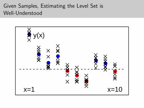
Given Samples, Estimating the Level Set isWell-Understood

y(x)

x=1 x=10

Given Samples, Estimating the Level Set isWell-Understood

●

●

●

●●

●

●●

●

●

y(x)

x=1 x=10

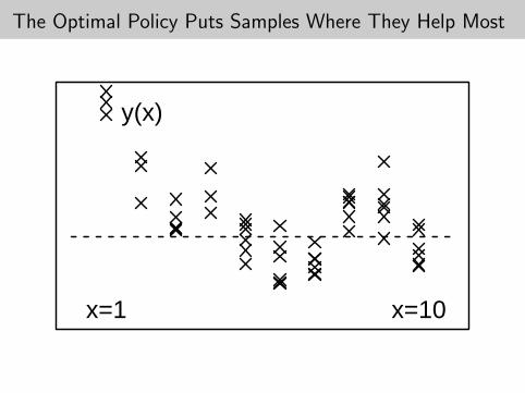
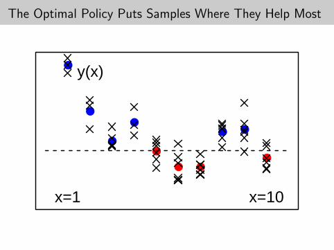
The Optimal Policy Puts Samples Where They Help Most

y(x)

x=1 x=10

The Optimal Policy Puts Samples Where They Help Most

y(x)

x=1 x=10

The Optimal Policy Puts Samples Where They Help Most

●

●

●

●● ●

●

● ●●

y(x)

x=1 x=10