Keywords: Gibbs sampler; MCMC methods; mixed-effects model; outliers; scale mixture of normal distributions; random effects
1. INTRODUCTION
Designs with repeated or grouped measures are common inepidemiological studies, economics, agronomy, forestry, and thepharmaceutical industry. Repeated-measures data are generatedby observing a number of subjects repeatedly under varying con-ditions. Usually, observations of the same subject are made at dif-ferent times, such as in longitudinal studies. Mixed-effects mod-eling is the most commonly used method for analysis of thistype of data. Mixed-effects models assume that the form of theintrasubject model that relates the response variable to time iscommon to all subjects, but some of the parameters that definethe model may vary with the subject. Mixed-effects models caneasily handle unbalanced repeated-measures data. The nonlinearmixed-effects (NLME) models are mixed-effects models in whichthe intrasubject model relating the response variable to time isnonlinear in the parameters.
A standard assumption regarding the NLME models is that ran-dom effects and within-subject errors are normally distributed.Widely available softwares, such as SAS Proc NLMIXED [1] andR package nlme [2], incorporate this assumption. Unfortunately,such normality assumptions are too restrictive and suffer fromthe lack of robustness against outlying observations. Accordingto Pinheiro et al. [3], outliers can arise either at the level of thewithin-subject error (�-outlier) or at the level of random effects(�-outlier). In the first case, some unusual within-subject valuesare observed, whereas in the second case, unusual subjects areobserved.
Most examples of the NLME models come from the areaof pharmacology, describing pharmacokinetic and pharmaco-dynamic (PK/PD) relationships. The well-known theophylline PKdataset (reported in [4]) is analyzed in this article. The data consist
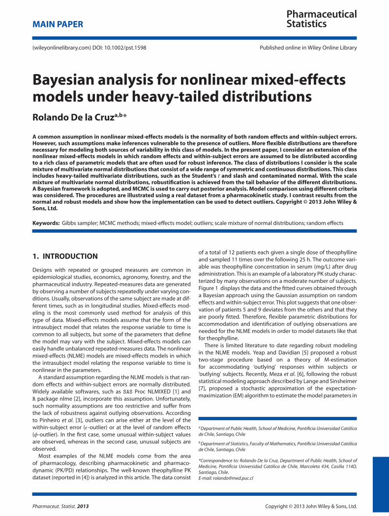
of a total of 12 patients each given a single dose of theophyllineand sampled 11 times over the following 25 h. The outcome vari-able was theophylline concentration in serum (mg/L) after drugadministration. This is an example of a laboratory PK study charac-terized by many observations on a moderate number of subjects.Figure 1 displays the data and the fitted curves obtained througha Bayesian approach using the Gaussian assumption on randomeffects and within-subject error. This plot suggests that one obser-vation of patients 5 and 9 deviates from the others and that theyare poorly fitted. Therefore, flexible parametric distributions foraccommodation and identification of outlying observations areneeded for the NLME models in order to model datasets like thatfor theophylline.
There is limited literature to date regarding robust modelingin the NLME models. Yeap and Davidian [5] proposed a robusttwo-stage procedure based on a theory of M-estimationfor accommodating ‘outlying’ responses within subjects or‘outlying’ subjects. Recently, Meza et al. [6], following the robuststatistical modeling approach described by Lange and Sinsheimer[7], proposed a stochastic approximation of the expectation-maximization (EM) algorithm to estimate the model parameters in
aDepartment of Public Health, School of Medicine, Pontificia Universidad Católicade Chile, Santiago, Chile
bDepartment of Statistics, Faculty of Mathematics, Pontificia Universidad Católicade Chile, Santiago, Chile
*Correspondence to: Rolando De la Cruz, Department of Public Health, School ofMedicine, Pontificia Universidad Católica de Chile, Marcoleta 434, Casilla 114D,Santiago, Chile.E-mail: [email protected]
Figure 1. Fitted curves for all 12 patients using normal assumptions on random effects and within-patient errors. The circles are the actual observations. The solid linesrepresent the fitted curves, and the bold circles on the curve are the fitted measurements.
the NLME models in which the Gaussian assumption for randomeffects and within-subject error is replaced by the scale mixtureof multivariate normal (SMMN) distributions. Here, I have demon-strated that the estimation can be implemented without muchdifficulty from a Bayesian point of view and have used the Gibbssampler and the Metropolis–Hastings algorithms to carry out theposterior analyses. In the literature, Lange and Sinsheimer [7], Liu[9], Choy and Smith [8], and Rosa et al. [10, 11] have observedthe robustness gained by using SMMN distributions in regressionanalysis. Therefore, our approach can be regarded as outlier-accommodating, although it also provides useful information foroutlier identification.
I organize the rest of the paper as follows. In Section 2, I brieflydescribe the class of SMMN distributions and define the membersof this class considered in the paper. In Section 3, I introduce theNLME models based on SMMN distributions. In Section 4, I con-sider the Bayesian method of estimation. I discuss model compar-ison in Section 5, and in Section 6, I present a real data applicationfrom a pharmacokinetic study. In Section 7, I present a study ofthe influence of a single outlier. Finally, Section 8 contains briefconcluding remarks.
2. PRELIMINARIES AND NOTATIONIn this section, I review a large family of distributions that will beconsidered in this paper, more specifically, the SMMN distribu-tions.
2.1. Scale mixture of multivariate normal distributions
In the sequel, I denote the d-dimensional multivariate normaldistribution with mean vector m, the covariance matrix M byNd.m, M/, and its PDF by �d.y; m, M/. Let Z � Nd.0, I/ and V arandom variable on Œ0,1/ with CDF H.vj�/ and PDF p.vj�), with� a scalar or vector valued parameter. I assume that Z and V areindependent and define a d-dimensional random variable
Y D �C V�1=2†1=2Z, (1)
where� 2 <d ,† is a positive definite symmetric matrix, and†1=2
is the square root of it. Then, the d-dimensional random variableY has a SMMN distributions (see [12]). Note that the expression (1)provides a useful tool for random number generation and fortheoretic purposes.
Alternatively, another way of representing the distribution (1) isthe following two-stage hierarchical representation
YjV D v � Nd.�, v�1†/,
V � H.�/.(2)
For convenience, I call � the location parameter, v the weight, †the scatter matrix, and � the hyperparameter. It follows from (2)that the marginal distribution of Y is given by
I use the notation SMMNd.�,†; H/ to indicate that Y has den-sity (3). When v D 1 and the mixing distribution function H isdegenerate, then SMMNd.�,†; H/ is a normal distribution. If thed-dimensional random variable Y has a SMMN distributions, itslinear transformations and marginal and conditional distributionsalso have a SMMN distributions.
If the moments of Z and V (the mixing variable) exist andare finite, from (2), using the iterative law of expectation, theexpectation and covariance matrix of Y are
E.Y/D E.E.YjV//D �,
cov.Y/D E.cov.YjV//C cov.E.YjV//D E.V�1/†.
The SMMN distributions provides a group of thick-tailed dis-tributions that are often used for robust inference. Three SMMNdistributions are commonly used for robust estimations: the mul-tivariate Student’s t, the multivariate slash, and the multivariatecontaminated multivariate normal distributions.
2.1.1. The multivariate Student’s t-distribution. The multivariateStudent’s t-distribution, Std.�,†, �/, with PDF
p.y/D�. �Cd
2 /
�. �2 /.��/d=2j†j�1=2
�1C
.y ��/0†�1.y ��/
�
��.�Cd/=2
,
y 2 <d ,(4)
where �, termed the degrees of freedom (DOF), � 2 <d thelocation parameter, and † the positive definite scatter matrixparameter, can be derived from the mixture model (3), by takingV to be distributed as �.�=2, �=2/with PDF
p.vj�/D.�=2/.�=2/
�.�=2/v.�=2/�1 exp
n��
2vo
, v > 0, � > 0,
where �.�/ is the standard gamma function. Here �.a, b/ denotesthe gamma distribution with shape parameter a and scale param-eter b. The expectation and covariance matrix of Y are E.Y/ D �
and cov.Y/ D .�=� � 2/†, � > 2. Some particular cases can beobtained from PDF (4). If � D 1, then (4) is the d-dimensionalCauchy distribution. If .� C d/=2 D s, an integer, then (4) is thed-dimensional Pearson type VII distribution. The limiting form of(4) as �!1 is the d-dimensional normal distribution with meanvector � and covariance matrix †. The Student’s t-distribution isan alternative choice for the normal distribution because it pro-vides more flexible tails than the normal distribution in modelingdiversified phenomena. The multivariate Student’s t-distributionhas been used for robust estimation in linear mixed-effects mod-els (see [3, 13–16]).
2.1.2. The multivariate slash distribution. Another SMMN distribu-tion, called multivariate slash distribution, arises when the distri-bution of V is ˇ.�, 1/with PDF
p.vj�/D �v��1, 0< v � 0, � > 0.
Here ˇ.c, d/ denotes the beta distribution with shape parametersc and d. Thus, from (3), the PDF of Y is given by
p. y;�,†, �/D j2�†j�1=2�
Z 1
0t�C
d2�1e�
ts2 dt
D
8̂̂̂̂<̂ˆ̂̂:
�j†j�1=22�Cd2 �.�C d
2 ; s=2/
.2�/d=2s�Cd2
, y ¤ �
j†j�1=2
.2�/d=2
2�
2�C d, y D �,
where �.a; z/ DR z
0 ta�1e�tdt is the incomplete gamma functionand s D . y � �/0†�1.y � �/. I use the notation Y � SL.�,†, �/if Y has a multivariate slash distribution with location parameter� 2 <d , positive definite scatter matrix parameter †, and DOF�. The expectation and covariance matrix of Y are E.Y/ D � andcov.Y/ D .�=� � 1/†, � > 1. For further details on multivariateslash distribution, see [7].
2.1.3. The contaminated multivariate normal distribution. Thecontaminated multivariate normal distribution, denoted byCNd.�,†, �1, �2/, is recovered from (3) by assuming that V , giventhe parameter vector � D .�1, �2/
Parameter �1 can be interpreted as the proportion of outliers,while �2 may be interpreted as a scale factor. The expectationand covariance matrix of Y are E.Y/ D � and cov.Y/ D .�1=�2 C
1��1/†. Applications and discussion of the contaminated normaldistribution are in [17].
2.1.4. Other scale mixture of multivariate normal distributions.There are other symmetric distributions that are members of theSMMN family. In a Bayesian framework, Choy and Smith [8] stud-ied the use of a member of such family as priors for the loca-tion parameter in a normal parametric model of the symmetricstable and exponential power distributions by means of normalscale mixtures. The multivariate logistic distribution has an SMMNdensity representation with an asymptotic Kolmogorov–Smirnovmixing distribution, whereas the generalized hyperbolic distri-bution has a generalized inverse Gaussian mixing distribution.However, these scale mixture of normal distributions requireexpertise in simulation methods, which hampers their applica-tions in statistical modeling.
Suppose I have m subjects with ni measurements obtained foreach, i D 1, : : : , m, and let n D
PmiD1 ni . Let yij denote the j-
th observed response for the i-th subject measured at time tij ,i D 1, : : : , m, j D 1, : : : , ni . In PK settings, tij is the time after drugadministration when the j-th drug concentration for the i-th sub-ject is measured. Let Yi D . yi1, : : : , yini /
0 denote the response vec-tor for the i-th subject recorded at known times ti D .ti1, : : : , tini /
0.In this article, I consider a general NLME model similar to thosepostulated by Lindstrom and Bates [18]. The form of the model is
where f is a nonlinear function of the subject-specific vectorregression parameters �i and represents the predicted vectorresponse of this subject at vector time ti , �i D .�i1, : : : , �ini /
0
denotes the vector of within-subject errors for the i-th subject,and it is assumed that �i � Nni .0, 2Ini /, where Ia denotes the.a � a/ identity matrix. The subject-specific vector regressionparameters �i are modeled as
�i D XiˇC bi , with biind� Nq.0,‰/, (7)
where ˇ is a p-dimensional vector of unknown fixed-effectsparameters, bi is a q-dimensional vector of unobservable random-effects parameters, Xi is a known design matrix of dimension.q�p/ associated with ˇ, and‰ is a covariance matrix. It is furtherassumed that �i and bi are mutually independent.
The NLME models (6) with the normality assumptions aboutthe random effects and within-subject errors are widely used inmany fields. However, such normality assumptions are vulnerableto the presence of atypical observations that can seriously affectthe estimation of fixed-effects and variance components. Thus,more distributions are necessary so that practitioners can havegreater flexibility when selecting a better model for a particulardataset. To overcome this obstacle, instead of normal assump-tions, I propose a rich class of parametric models for randomeffects and within-subject error in NLME models. The class of dis-tributions I consider is the SMMN distributions. Thus, the model isexpressed as
Yij�iind� SMMNni
�f .�i , ti/,
2Ini ; H1
�,
�iind� SMMNq.Xiˇ,‰; H2/, iD 1, : : : , n.
(8)
It follows that the joint density of observations and randomeffects is given by
p. y,�j2,‰, �, /DmY
iD1
p. yij�i , 2, �/p.�ijˇ,‰, /
D
mYiD1
�Z 10
p. yijvi ,�i , 2, �/p.vij�/dvi
��
�Z 10
p.�ijwi ,ˇ,‰, /p.wij/dwi
�D
mYiD1
�.2�2/�ni=2
Z 10
vni=2i exp
��
1
2viı
2i . yi ,�i/
�p.vij�/dvi
��
�j2�‰j�1=2
Z 10
wq=2i exp
��
1
2wi�
2i .�i ,ˇ/
�p.wij/dwi
�,
where y D�
Y01, Y02, : : : , Y0m0
, � D��01,�02, : : : ,�0m
0, ı2
i . yi ,�i/ D
�2jjyi � fi.�i , ti/jj2, and�2
i .�i ,ˇ/D .�i � Xiˇ/0‰�1.�i � Xiˇ/.
For convenience, using the two-stage hierarchical representa-tion (2), I can rewrite model (8) as
Yij�i , viind� Nni
�f .�i , ti/, v�1
i 2Ini
�, vi
ind� H1.�/
�ijwiind� Nq
�Xiˇ, w�1
i ‰�
, wiind� H2./,
(9)
for iD 1, : : : , n, where the latent variables vi and wi are presumedto be mutually independent.
Using the multivariate Student’s t-distribution with the par-ticular case H1 D H2, Pinheiro et al. [3] considered a robustextension of the linear mixed-effects models. They presented sev-eral comparably efficient EM type algorithms for computing themaximum likelihood estimates and illustrated the robustness ofthe model via a real example and some simulations. Also, usingH1 D H2, Lachos et al. [19] considered a Bayesian approachfor linear and NLME models with censored responses where theGaussian assumption for random effects and within-subject erroris replaced by SMMN distributions. Although these distributionalassumptions allow for the accommodation of outliers, in its for-mulation, it is assumed that the mixture distributions for the twosources of variability in the model have the same shape and sharethe same parameters. Some authors (see, e.g., [20, 21]) empha-size that this assumption may be very difficult to justify. In thiswork, I assume that the mixture variables associated with errorsand random effects are different.
Exp, exponential distribution; U, uniform distribution; � , gamma distribution.
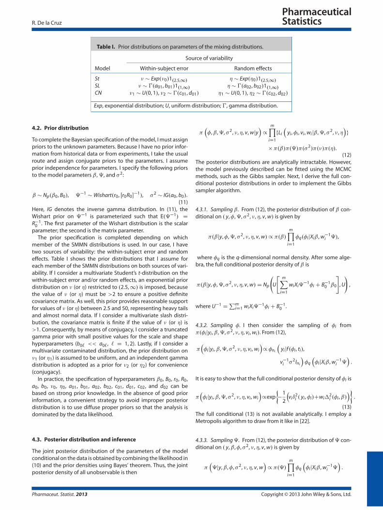
4.2. Prior distribution
To complete the Bayesian specification of the model, I must assignpriors to the unknown parameters. Because I have no prior infor-mation from historical data or from experiments, I take the usualroute and assign conjugate priors to the parameters. I assumeprior independence for parameters. I specify the following priorsto the model parameters ˇ,‰, and 2:
(11)Here, IG denotes the inverse gamma distribution. In (11), theWishart prior on ‰�1 is parameterized such that E.‰�1/ D
R�10 . The first parameter of the Wishart distribution is the scalar
parameter; the second is the matrix parameter.The prior specification is completed depending on which
member of the SMMN distributions is used. In our case, I havetwo sources of variability: the within-subject error and randomeffects. Table I shows the prior distributions that I assume foreach member of the SMMN distributions on both sources of vari-ability. If I consider a multivariate Student’s t-distribution on thewithin-subject error and/or random effects, an exponential priordistribution on � (or ) restricted to .2.5,1/ is imposed, becausethe value of � (or ) must be >2 to ensure a positive definitecovariance matrix. As well, this prior provides reasonable supportfor values of � (or ) between 2.5 and 50, representing heavy tailsand almost normal data. If I consider a multivariate slash distri-bution, the covariance matrix is finite if the value of � (or ) is>1. Consequently, by means of conjugacy, I consider a truncatedgamma prior with small positive values for the scale and shapehyperparameters (b0` << a0`, ` D 1, 2). Lastly, if I consider amultivariate contaminated distribution, the prior distribution on�1 (or 1) is assumed to be uniform, and an independent gammadistribution is adopted as a prior for �2 (or 2) for convenience(conjugacy).
In practice, the specification of hyperparameters ˇ0, B0, r0, R0,a0, b0, �0, 0, a01, b01, a02, b02, c01, d01, c02, and d02 can bebased on strong prior knowledge. In the absence of good priorinformation, a convenient strategy to avoid improper posteriordistribution is to use diffuse proper priors so that the analysis isdominated by the data likelihood.
4.3. Posterior distribution and inference
The joint posterior distribution of the parameters of the modelconditional on the data is obtained by combining the likelihood in(10) and the prior densities using Bayes’ theorem. Thus, the jointposterior density of all unobservable is then
���,ˇ,‰, 2, �, , v, wjy
�/
mYiD1
fLi
�yi ,�i , vi , wijˇ,‰, 2, �,
�g
� �.ˇ/�.‰/�.2/�.�/�./.(12)
The posterior distributions are analytically intractable. However,the model previously described can be fitted using the MCMCmethods, such as the Gibbs sampler. Next, I derive the full con-ditional posterior distributions in order to implement the Gibbssampler algorithm.
4.3.1. Sampling ˇ. From (12), the posterior distribution of ˇ con-ditional on . y,�,‰, 2, �, , v, w/ is given by
�.ˇjy,�,‰, 2, �, , v, w// �.ˇ/mY
iD1
�q.�ijXiˇ, w�1i ‰/,
where �q is the q-dimensional normal density. After some alge-bra, the full conditional posterior density of ˇ is
�.ˇjy,�,‰, 2, �, , v, w/D Np
U
"mX
iD1
wiXi‰�1�i C B�1
0 ˇ0
#, U
!,
where U�1 DPm
iD1 wiXi‰�1�i C B�1
0 .
4.3.2. Sampling �. I then consider the sampling of �i from�.�ijyi ,ˇ,‰, 2, �, , vi , wi/. From (12),
���ijyi ,ˇ,‰, 2, �, , vi , wi
�/ �ni
�yijf .�i , ti/,
v�1i 2Ini
��q
��ijXiˇ, w�1
i ‰�
.
It is easy to show that the full conditional posterior density of �i is
���ijyi ,ˇ,‰, 2, �, , vi , wi
�/exp
��
1
2
�viı
2i . yi ,�i/Cwi�
2i .�i ,ˇ/
��.
(13)The full conditional (13) is not available analytically. I employ aMetropolis algorithm to draw from it like in [22].
4.3.3. Sampling‰. From (12), the posterior distribution of‰ con-ditional on . y,ˇ,�, 2, �, , v, w/ is given by
where IW denotes the inverse Wishart distribution.
4.3.4. Sampling 2. From (12), the full conditional posterior den-sity �.2jy,ˇ,�,‰, �, , v, w/ is given by
��2jy,ˇ,�,‰, �, , v, w
�/�
�2� mY
iD1
�ni
�yijf .�i , ti/, v�1
i 2Ini
�.
Defining A0 D 2b0=.b0Pm
iD1 vijjyi � fi.�i , ti/jj2 C 2/, it is easy to
show that the full conditional posterior density of 2 is
��2jy,ˇ,�,‰, �, , v, w
�D IG
NC 2a0
2, A0
�.
4.3.5. Sampling v and �. For i D 1, : : : , m, the vi are condition-ally independent. Thus, the sampling of v can be made throughcomponent-wise drawing of vi from �.vijy,ˇ,�,‰, 2, �, , w/. Ingeneral,
��
vijy,ˇ,�,‰, 2, �, , w�/ �ni
�yijf .�i , ti/, v�1
i 2Ini
��.vij�/.
(14)For parameters �, the full conditional posterior density has theform
���jy,ˇ,�,‰, 2, , v, w
�/ �.�/
mYiD1
�.vij�/. (15)
Sampling from (14) and (15) depends on the SMMN distributionadopted for the within-subject error. Next, I review these full con-ditional densities for the specific SMMN distributions consideredin this paper.
Multivariate Student’s t-distribution. In the case that the specificSMMN distribution on within-subject error is the multivariate Stu-dent’s t-distribution, vij� � �.�=2, �=2/. With this setting, the fullconditional posterior density of vi is
��
vijy,ˇ,�,‰, 2, �, , w�D �
ni C �
2,ı2
i . yi ,�i/C �
2
!,
���jy,ˇ,�,‰, 2, , v, w
�/ c.�/�
m�
2C 2,
1
2
mXiD1
� .vi � log vi/
!1.2.5,1/,
where c.�/ D Œe�=m2�=2�.�=2/��m. This distribution does nothave a closed form, but a Metropolis–Hastings step can beembedded in the MCMC scheme to obtain draws for �.
Multivariate slash distribution. Assuming a multivariate slash dis-tribution for the within-subject error, I have vij� � ˇ.�, 1/. Thus,from (14), the full conditional posterior density of vi is
��
vijy,ˇ,�,‰, 2, �, , w�D t�
ni
2C �,
ı2i . yi ,�i/
2, t1
!.
where tGamma denotes the truncated gamma distribution withthe right truncation point at t1 D 1. Further, the full conditionalposterior density of � is
���jy,ˇ,�,‰, 2, , v, w
�D �
mC a1, b1 �
mXiD1
log vi
!1.1,1/.
The Gibbs sampler is straightforward for the multivariate slash dis-tribution because all the conditional posterior distributions haveclosed forms.
Contaminated multivariate normal distribution. If a contaminatedmultivariate normal distribution is adopted for the within-subjecterror, the possible states of the ‘weights’ vi are �1 or 1. Its PDFis given in (5). Then, from (14), I have that the full conditionalposterior distribution of each wi is proportional to8̂<̂
:�
ni=22 �1 exp
���2
2ı2
i . yi ,�i/�
if vi D �2
.1� �1/ exp
�
1
2ı2
i . yi ,�i/
�if vi D 1,
and the conditional probabilities are arrived at readily by suitablenormalization. Note that the PDF (5) can be rewritten as
p.vij�1, �2/D �Œ.1�vi/=.1��2/�1 .1� �1/
Œ.vi��2/=.1��2/�.
Then, the full conditional posterior density of the proportion ofoutliers �1 is
���1jy,ˇ,�,‰, 2, , �2, v, w
�D ˇ
a2C
1
1� �2
mXiD1
.1� vi/, b2
C1
1� �2
mXiD1
.vi � �2/
!.
To update �2, a Metropolis–Hastings algorithm is adopted follow-ing the approach described in [11].
4.3.6. Sampling w and . Like the vector of weights v, the com-ponents wi of the vector of weights w are conditionally indepen-dent. Thus, the sampling of w can be carried out as with v throughcomponent-wise drawing of wi from �.wijy,ˇ,�,‰, 2, �, , v/.From (12), I have that the full conditional posterior densities ofwi and have the forms
��
wijy,ˇ,�,‰, 2, �, , v�/ �q
��ijXiˇ, w�1
i ‰��.wij/ (16)
and
��jy,ˇ,�,‰, 2, �, v
�/ �./
mYiD1
�.wij/. (17)
As in Section 4.3.5, sampling from (16) and (17) depends on whatdistribution I assume for the random effects. The procedure tocalculate these full conditional posterior densities is similar tothat described in Section 4.3.5. Next, I show the full conditionalposterior densities for each member of the SMMN distributionsconsidered in this paper.
Multivariate Student’s t-distribution. The full conditional densitiesfor wi and are given by
��
wijy,ˇ,�,‰, 2, �, , v�D �
qC
2,�2
i .�i ,ˇ/C
2
!
and
��jy,ˇ,�,‰, 2, �, v, w
�/ c./�
m
2C 2,
1
2
mXiD1
� .wi � log wi/
!1.2.5,1/,
where c./ Dh
e�=m2�=2�.=2/i�m
. This distribution does
not have a closed form, but a Metropolis–Hastings step can beembedded in the MCMC scheme to obtain draws for .
Multivariate slash distribution. Here, the full conditional densitiesfor wi and are
��
wijy,ˇ,�,‰, 2, �, , v�D t�
q
2C ,
�2i .�i ,ˇ/
2, t1
!,
and
��jy,ˇ,�,‰, 2, �, v, w
�D �
mC a1, b1 �
mXiD1
log wi
!1.1,1/,
where tGamma is the truncated gamma distribution with theright truncation point at t1 D 1.
Contaminated multivariate normal distribution. The full condi-tional distribution of each wi is proportional to8̂<̂
:
q=22 �1 exp
��2
2�2
i .�i ,ˇ/�
if wi D 2
.1� 1/ exp
�
1
2�2
i .�i ,ˇ/
�if wi D 1,
and the conditional probabilities are arrived at readily by suit-able normalization. Further, the full conditional posterior densityof the proportion of outliers 1 is
��1jy,ˇ,�,‰, 2, 2, �, v, w
�D ˇ
a2C
1
1� 2
mXiD1
.1�wi/, b2
C1
1� 2
mXiD1
.wi � 2/
!.
To update 2, a Metropolis–Hastings algorithm is adopted follow-ing the approach described in [11].
4.4. Predictive distributions
Let O D f. yi , ti/ D . yij , tij , j D 1, : : : , ni/gmiD1 be the set of all
observed measurements. Suppose that I want to predict the .nf �
1/ response vector yf for another subject. Let p. yf j , xf / denotethe sampling density for yf , and the predictive distribution foryf is
p. yf jO/D p. yf jxf ,O/DZ
p. yf j , xf /p. jO/d , (18)
where denotes the vector of all parameters in the model. Theintegration is usually analytically intractable. Therefore, I con-struct a set of MCMC samples f .t/; t D 1, : : : , Tg from theirposterior distribution and use
p. yf jO/�1
T
TXtD1
p. yf j .t/, xf /
to approximate expression (18). In general, I use the sample mean
of MCMC samplesn
y.t/f , tD 1 : : : , To
as the prediction of yf .
5. MODEL COMPARISON
To compare candidate models, I compute p. yijO�i/, which isthe posterior predictive density for subject i conditional on O�i ,which in turn is the observed dataset with the data of subject ideleted. This value is known as the conditional predictive ordinate(CPO; [23, 24]) and has been widely used for model diagnosticsand assessment.
For subject i, the CPO statistics under model M`, 1 � ` � L isdefined as
CPOi.M`/D p . yijO�i ,M`/
D E�` .p. yij `/jO�i/ ,
where �i denotes the exclusion of the data from subject i. The `is the set of parameters of model M`, and p. yij `/ is the sam-pling density of the model evaluated at the i-th observation. Thepreceding expectation is taken with respect to the posterior dis-tribution of the model parameters ` given the cross-validateddata O�i . For subject i, the CPOi.M`/ can be obtained from theMCMC samples by computing the following weighted average:
bCPOi.M`/D
0@ 1
T
TXtD1
1
p�
yij .t/`
�1A�1
,
where T is the number of simulations. The .t/`
denotes the param-eter samples at the t–th iteration. A large CPO value indicatesa better fit. A useful summary statistic of the CPOi.M`/ is thelogarithm of the pseudomarginal likelihood (LPML), defined asLPML D
PmiD1 log.bCPOi.M`//. Models with greater LPML values
represent a better fit. The LPML is well defined under the poste-rior predictive density, and it is computationally stable. The LPMLhas been used extensively in Bayesian analysis for model selectionin situations of simpler and more complicated models and has along history in statistics literature (see [23, 25–27]). Model com-parison can also be performed using summary measures. Sup-pose that I have two models M1 and M1 under consideration.The pseudo-Bayes factor (PsBF), a surrogate for the Bayes factorbased on the CPO for comparing the two models, is defined as
PsBF .M1,M2/D
mYiD1
bCPOi.M1/
bCPOi.M2/.
Another tool for model comparison is the deviance informationcriterion (DIC) statistic, introduced by Spiegelhalter et al.[28]. TheDIC is defined as
where N ` is the vector of average values for all parameters inmodel M` at the end of the sampling process
D. N `/D�2 log p. yj N `/,
NDD�2
ZŒlog p. yj `/�p. `jy/d `
D E�`jy .D. `// ,
where ` is the sample value of all unknown parameters in modelM` in a given MCMC iteration. The DIC combines a measureof model fit ( ND) and a measure of model complexity (D. N `/)(see [28]). Lower values of the criterion indicate better fittingmodels. The DIC is approximately equivalent to the AIC in mod-els with negligible prior information [28]. Discussion of the DICas a criterion for posterior predictive model comparison is givenin [29].
6. THE THEOPHYLLINE KINETICS DATASET
This section illustrates the proposed method by reanalyzing thetheophylline dataset presented in [2]. The dataset consists of theoral doses of the anti-asthmatic drug theophylline administeredto 12 patients. Serum concentrations were measured at 11 timepoints over the next 25 h after drug administration. Figure 1presents the time profile for these 12 patients. The longitudinalobservations of each patient exhibit a nonlinear profile. The PK ofthis drug is modeled by the first-order open-compartment model(iD 1, : : : , 12, jD 1, : : : , 11)
Cij DDiKeiKai
Cli.Kai � Kei/
˚exp.�Keitij/� exp.�Kaitij/
�C �ij , (19)
where Cij is the theophylline concentration serum (mg/L) forpatient i measured at time tij , with an initial dose of theophylline
Di , and Kei , Kai , and Cli are unknown patient-specific parametersrepresenting the elimination rate, absorption rate, and clearance,respectively.
The model (19) is known as the ‘flip-flop’ model because thereis nonidentifiability; the parameters .Kei , Kai , Cli/
0 give the samecurve as the parameters .Kai , Kei , Cli/
0. To enforce identifiability, itis typical to assume that Kai > Kei > 0. I assume this constraint viaparametrization:
�1i D log Kei D ˇ1C bi1
�2i D log.Kai � Kei/D ˇ2C bi1
�3i D log Cli D ˇ3C bi3.
In principle, I assume the usual assumption bi D .bi1, bi2, bi3/0 �
N3.0,‰/ and �i D .�i1, : : : , �ini /0 � N11.0, 2I11/, which I name the
N–N NLME model.In order to implement the Gibbs sampler algorithm, I chose
the values of the hyperparameters in such a way as toobtain noninformative priors. The values of the components ofR0 were chosen following the strategy of Wakefield et al. [30](see also [22]). I used 85,000 iterations with 10,000 sweeps asburn-in. Samples were collected at a spacing of 15 iterationsto obtain approximately independent samples. Finally, I totaledBD 5, 000 posterior Monte Carlo samples. To monitor the conver-gence of the Gibbs sampler, I used the methods recommendedby Cowles and Carlin [31]. Graphical diagnostics were plotted toevaluate the model adequacy of the N–N NLME model. From a fre-quentist viewpoint, Pinheiro et al.[3] used Mahalanobis distancesı2
i . yi ,�i/ and �2i .�i ,ˇ/ to detect outlying observations. They
defined the quantities ı2i . yi ,�i/=ni and �2
i .�i ,ˇ/=q to identifyoutlying observations. These statistics a priori have expected val-ues equal to 1. Posterior estimates of these quantities can be eas-
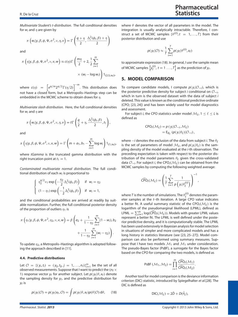
ily calculated using samples of the posterior as ı2.b/i . yi ,�
.b/i /=ni
Figure 2. Posterior Mahalanobis distances for within-patient vector error and random effects of patient i, iD 1, : : : , 12, for the N–N nonlinear mixed-effects model.
.b/i ,ˇ.b//=q, b D 1, : : : , B, where B is the number of
samples. Figure 2 presents the posterior mean of these diagnos-tic statistics, which suggests that patients 2 and 5 are �-outliers,and patients 1 and 9 are possibly �-outliers.
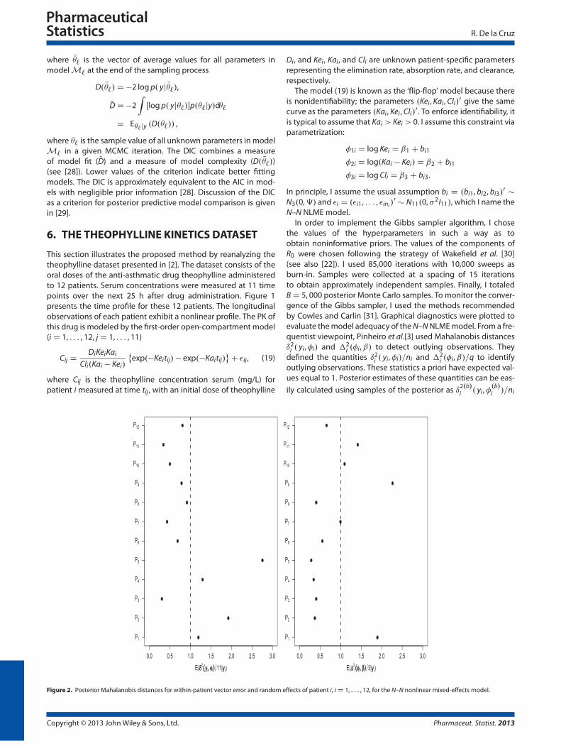
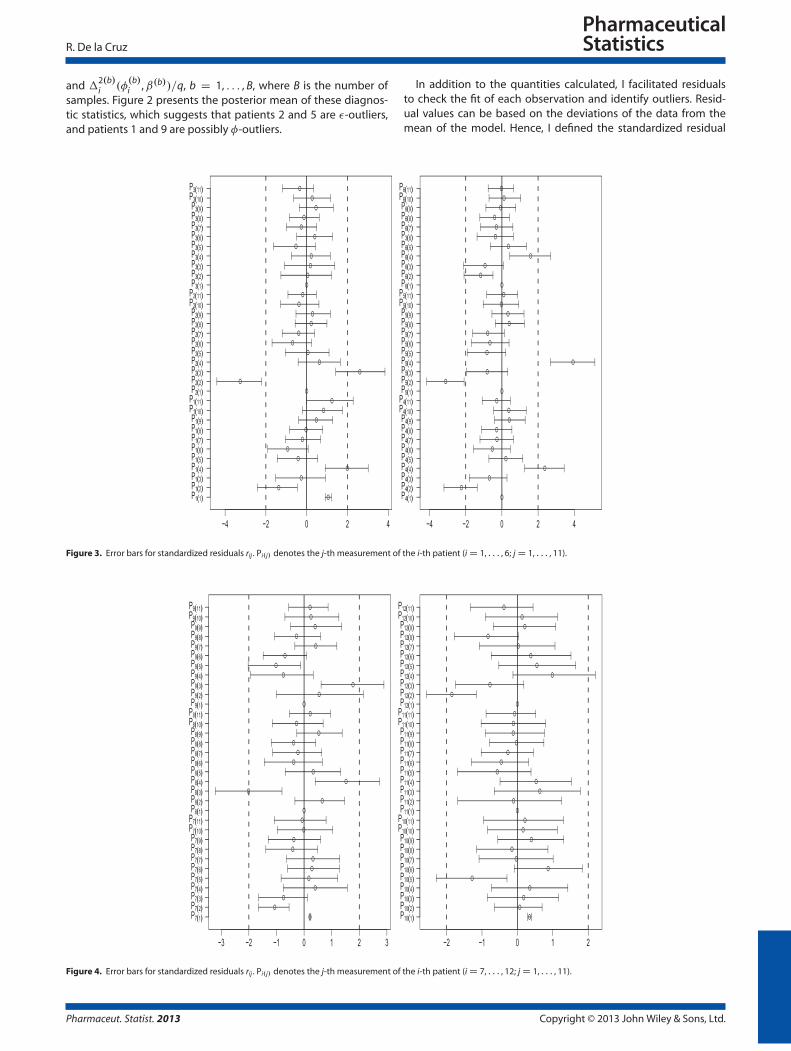
In addition to the quantities calculated, I facilitated residualsto check the fit of each observation and identify outliers. Resid-ual values can be based on the deviations of the data from themean of the model. Hence, I defined the standardized residual
Figure 3. Error bars for standardized residuals rij . Pi.j/ denotes the j-th measurement of the i-th patient (iD 1, : : : , 6; jD 1, : : : , 11).
Figure 4. Error bars for standardized residuals rij . Pi.j/ denotes the j-th measurement of the i-th patient (iD 7, : : : , 12; jD 1, : : : , 11).
Var. yijj /. For our N–N NLME model,the standardized residuals rij are a priori normal with mean zeroand variance units. Posterior to the standardized residuals, rij
can be formed from samples of the posterior as r.b/ij D . yij �
E. yijj .b///=
qVar. yijj .b//, b D 1, : : : , B. Error bars of the poste-
rior residual values are provided in Figures 3 and 4. Reference linesat values of �2 and 2 are added to trace outlier values. Clearly,patients 2 and 5 present large residuals, and measurements 2 and
3 of patient 2 and measurements 2 and 4 of patient 5 have abso-lute error values close to the value of 2 with error bars includingthis values. These results agree with those found in Figure 2. I canalso see that patients 1, 4, 8, and 12 present some large residu-als with error bars including value 2. A few large residuals withinthe first 2 h after drug administration might have been causedby intense observations in the process of absorption and sparseobservations in the process of elimination. The results show thata better model is necessary for this particular dataset.
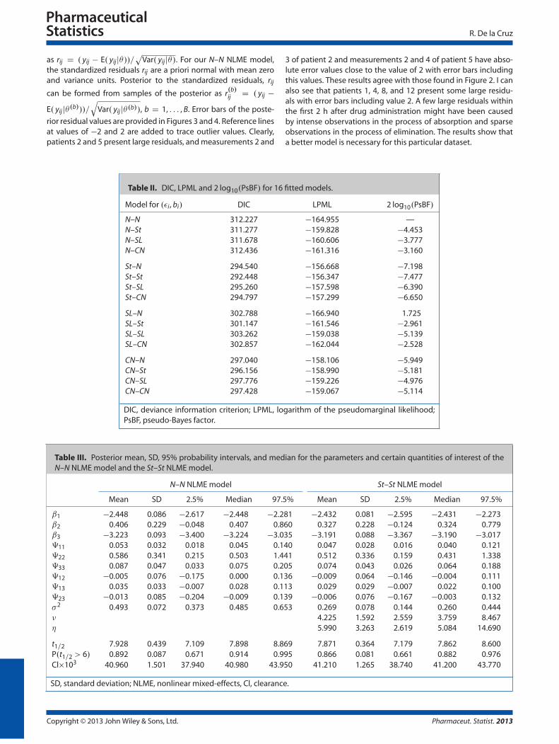
Table II. DIC, LPML and 2 log10.PsBF/ for 16 fitted models.
DIC, deviance information criterion; LPML, logarithm of the pseudomarginal likelihood;PsBF, pseudo-Bayes factor.
Table III. Posterior mean, SD, 95% probability intervals, and median for the parameters and certain quantities of interest of theN–N NLME model and the St–St NLME model.
N–N NLME model St–St NLME model
Mean SD 2.5% Median 97.5% Mean SD 2.5% Median 97.5%
As well as the N–N NLME model, depending on which sourceoutliers arise from, there are 15 types of NLME models that canbe considered, among them are the normal–Student’s t (N–St),normal–slash (N–SL), normal–contaminated normal (N–CN), andStudent’s t–normal (St–N). For example, the N–St is an NLMEmodel with normally distributed within-subject error terms andStudent’s t-distributed random effects in situations where out-liers arise solely from random effects. Through the comparisonsof these 16 models, not only could I identify influential outliersbut also determine the source from which identified outliers arise.I compared the 16 models using DIC, LPLM, and log PsBF. FromTable II, the St–St NLME model was considered best among all themodels considered.
Table III lists posterior summaries of the parameters for theN–N NLME model and the St–St NLME model. The estimated DOFare between 4 and 6, suggesting that both distributions for thewithin-patient error terms and random effects are heavy-tailed.This confirmed the findings in the preliminary analysis earlier.Note that the 2 log10 PsBF for the N–N NLME model versus theSt–St NLME model was �7.5. Therefore, the improvement of theSt–St NLME model over the N–N NLME model is noticeable.
One of the principal aims of this analysis is the detection of out-lying patients by using the weights vi and wi in the St–St NLMEmodel. The prior expectation of vi and wi is 1, so that vi and wi
values substantially below 1 indicate that the i-th patient is an�-outlier and a �-outlier, respectively. Figure 5 displays the 95%credible interval (CI) of the posterior sample values of vi and wi
for each of the 12 patients. It is clear that patients 2 and 5 are �-outliers. Although the CI of patients 1, 4, and 8 contain the value1, they have a small weight, see Figure 5(a), which indicates thatthese patients are possible �-outliers. These results agree withthose found in Figures 3 and 4. From Figure 5(b), patients 1 and9 are possible �-outliers. To discover the reason why patients 1
and 9 had small weights, patient components of the random-effects vectors were examined. A scatterplot of the medians of therandom effects for elimination, absorption, and clearance withpatient number as a plotting symbol shows that patient 1 hada low elimination rate and clearance, and patient 9 had a highabsorption rate.
There is interest in pharmacokinetics in quantities such asthe clearance (Cl) and the terminal half-life t1=2 D log 2=Kei .Because log Kei � St1.ˇ1,‰11, /, then log t1=2 � St1.log.log 2/�ˇ1,‰11, /. Table III shows the posterior summaries of thesequantities. The probability of a patient selected from the popu-lation having a half-life greater than 6 h is also included. Similarresults were obtained for the St–St and N–N NLME models, andthe only difference in the estimations of the standard deviationsbeing that they were lower for the former.
7. STUDY OF INFLUENCE OF ASINGLE OUTLIER
The robustness of the NLME model defined in Section 3 withrespect to the N–N NLME model can also be assessed throughthe influence of a single outlying observation on the estimatedparameters. Of the 15 robust models discussed in Section 6, Iconsidered only the St–St NLME model to compare with theN–N NLME model in order to study the influence of a singleoutlying observation on the estimated parameters. I simulated adataset considering the model (19) (i D 1, : : : , 12, j D 1, : : : , 11)using the same time points and dose of the theophylline dataset,and with normal distributional assumptions on both randomeffects and within-patient errors.
I considered the influence of a change of � units in a singlemeasurement on the estimated parameters. Thus, in the
Figure 5. Posterior summaries for the weights (a) vi and (b) wi of patient i, iD 1, : : : , 12. Posterior distributions substantially below the line of unity indicate outlying patients.
Figure 6. Percentage change in estimates under the N–N and St–St NLME models for different contaminations� of a single observation. The solid line represents the St–Stmodel and the dashed line the N–N model.
simulated dataset, I contaminated the fourth measure ofthe eighth patient, that is, Y8j.�/ D Y8j C �, with j D 4, andvaried � between �12 and 12 mg/L by increments of2 mg/L. I estimated the parameters of the models for eachchange of � and recorded the relative change in the estimates.b .�/ � b /=b , where b denotes the estimates without con-tamination and b .�/ the estimates for the contaminated data.Because 2 and ‰ have different interpretations under theN–N NLME and St–St NLME models, I considered that vi �
�.�=2, .� � 2/=2/ in order to obtain E. yij / D 2I11 under boththe N–N and St–St NLME models. Thus, I could compare 2 underboth models.
Figure 6 presents the results of the relative changes of theestimates of ˇ D .ˇ1,ˇ2,ˇ3/
0, 2 and the standard deviations ofˇr (r D 1, 2, 3). As expected, the estimates from the St–St NLMEmodel are less affected by the variations of � than those fromthe N–N NLME model. As with the results found by Pinheiro etal.[3] in the LME model, the influence of a single observation isunbounded in the case of the N–N NLME model but bounded inthe St–St NLME model. The outlying observation has more impacton the estimates of 2 in both models.
For closer contamination values (j�j � 2), the fit under bothNLME models is almost identical and therefore has similar influ-ence curves. The estimates under the two models are identical forthe uncontaminated simulated dataset.
8. DISCUSSION
In this paper, NLME models have been analyzed under theassumption that within-subject error terms and random effectsare distributed according to a rich class of parametric models.Based on the SMMN distributions, the NLME models can accom-modate different types of outliers and allow practitioners toanalyze data in a wide variety of considerations. As I have shownearlier, the models can be straightforwardly implemented undera Bayesian framework because of their hierarchical representationof SMMN distributions. I have demonstrated our approach with areal dataset and have shown that the heavy-tailed models havebetter performance than their Gaussian competitor. One impor-tant feature of the SMMN distributions is that posterior meansof the mixing parameters can be used as global indicators ofpossible outliers and to determine from which source influentialoutliers arise.
A small simulation study shows the gains in efficiency for theSt–St NLME model relative to the N–N NLME model under outliercontamination.
The class of SMMN distributions provides a group of thick-taileddistributions that are often used for robust inference, but skew-ness is present in many datasets. Therefore, it is necessary to con-sider flexible parametric distributions that account for this issue.The scale mixtures of skew-normal distributions [32] is a class of
skew-thick-tailed distributions that extend the class of SMMN dis-tributions. Thus, a generalization of this work is to consider theNLME models using the scale mixtures of skew-normal distribu-tions. The SMMN distributions provide an alternative to usinga nonparametric model, such as a Dirichlet process, as a priorfor modeling the within-subject variability and/or random effects(see, e.g., [33, 34]).
Acknowledgement
This research was supported by the Fondo Nacional deDesarrollo Científico y Tecnológico (FONDECYT) grants 11080017and 1120739.
REFERENCES
[1] Littell RC, Milliken GA, Stroup WW, Wolfinger RD, Schabenberger O.SAS for mixed models, Second Edition. SAS Institute Inc.: Cary, NC,USA, 2006.
[2] Pinheiro J, Bates DM. Mixed-effects models in S and S-PLUS. Springer:New York, 2000.
[3] Pinheiro J, Liu C, Wu Y. Efficient algorithms for robust estimationin linear mixed-effects models using the multivariate t distribution.Journal of Computational and Graphical Statistics 2001; 10:249–276.
[4] Boeckmann AJ, Sheiner LB, Beal SL. NONMEM users guide—part V.NONMEM Project Group, University of California: San Francisco,1994.
[5] Yeap BY, Davidian M. Robust two-stage estimation in hierarchicalnonlinear models. Biometrics 2001; 57:266–272.
[6] Meza C, Osorio F, De la Cruz R. Estimation in nonlinear mixed-effectsmodels using heavy-tailed distributions. Statistics and Computing2012; 22:121–139.
[7] Lange K, Sinsheimer J. Normal/independent distributions and theirapplications in robust regression. Journal of Computational andGraphical Statistics 1993; 2:175–198.
[8] Choy STB, Smith AFM. Hierarchical models with scale mixtures ofnormal distributions. Test 1997; 6:205–221.
[9] Liu C. Bayesian robust multivariate linear regression with incom-plete data. Journal of the American Statistical Association 1996;91:1219–1227.
[10] Rosa GJM, Padovani CR, Gianola D. Robust linear mixed models withnormal/independent distributions and Bayesian MCMC implemen-tation. Biometrical Journal 2003; 45:573–590.
[11] Rosa GJM, Gianola D, Padovani CR. Bayesian longitudinal data anal-ysis with mixed models and thick-tailed distributions using MCMC.Journal of Applied Statistics 2004; 31:855–873.
[12] Andrews DF, Mallows CL. Scale mixtures of normal distributions.Journal of the Royal Statistical Society, Series B 1974; 36:99–102.
[13] Lin TI. Longitudinal data analysis using t linear mixed modelswith autoregressive dependence structures. Journal of Data Science2008; 6:333–355.
[14] Lin TI, Lee JC. A robust approach to t linear mixed models applied tomultiple sclerosis data. Statistics in Medicine 2006; 25:1397–1412.
[15] Song PX-K, Zhang P, Qu A. Maximum likelihood inference in robustlinear mixed-effects models using multivariate t distributions. Sta-tistica Sinica 2007; 17:929–943.
[16] Staudenmayer J, Lake EE, Wand MP. Robustness for general designmixed models using the t-distribution. Statistical Modelling 2009;9:235–255.
[17] Little RJA. Robust estimation of the mean and covariance matrixfrom data with missing values. Applied Statistics 1988; 37:23–38.
[19] Lachos VH, Bandyopadhyay D, Dey DK. Linear and nonlinearmixed-effects models for censored HIV viral loads using nor-mal/independent distributions. Biometrics 2011; 67:1594–1604.
[20] Jara A, Quintana F, San Martin E. Linear mixed models with skew-elliptical distributions: a Bayesian approach. Computational Statis-tics and Data Analysis 2008; 52:5033–5045.
[21] Lin TI, Lee JC. Estimation and prediction in linear mixed modelswith skew-normal random effects for longitudinal data. Statistics inMedicine 2007; 27:1490–1507.
[22] Wakefield J. The Bayesian analysis of population pharmacoki-netic models. Journal of the American Statistical Association 1996;91:62–75.
[23] Chen M-H, Shao Q-M, Ibrahim JG. Monte Carlo methods in Bayesiancomputation. Springer-Verlag Inc: New York, 2000.
[24] Gelfand AE, Dey DK, Chang H. Model determination using predic-tive distributions with implementation via sampling based meth-ods (with discussion). Bayesian statistics 4, Bernardo JM, Berger JO,Dawid AP, Smith AFM (eds). Oxford University Press: Oxford, 1992;147–167.
[25] Brown ER, Ibrahim JG. Bayesian approaches to joint-cure rate andlongitudinal models with applications to cancer vaccine trials. Bio-metrics 2003; 59:686–693.
[26] Brown ER, Ibrahim JG, DeGruttola V. A flexible B-spline modelfor multiple longitudinal biomarkers and survival. Biometrics 2005;61:64–73.
[27] Ghosh P, Tu W. Assessing sexual attitudes and behaviors of youngwomen: a joint model with nonlinear time effects, time varyingcovariates, and dropouts. Journal of the American Statistical Associ-ation 2009; 104:474–485.
[28] Spiegelhalter DJ, Best NG, Carlin BP, van der Linde A. Bayesian mea-sures of model complexity and fit (with discussion). Journal of theRoyal Statistical Society, Series B 2002; 64:583–639.
[29] van der Linde A. DIC in variable selection. Statistica Neerlandica2005; 59:45–56.
[30] Wakefield JC, Smith AFM, Racine–Poon A, Gelfand AE. Bayesiananalysis of linear and non-linear population models by usingthe Gibbs sampler. Journal of the Royal Statistical Society. Series C(Applied Statistics) 1994; 43:201–221.
[31] Cowles MK, Carlin BP. Markov chain Monte Carlo convergence diag-nostics: a comparative review. Journal of the American StatisticalAssociation 1996; 91:883–904.
[32] Branco MD, Dey DK. A general class of multivariate skew-ellipticaldistributions. Journal of Multivariate Analysis 2001; 79:99–113.
[33] de la Cruz–Mesía R, Quintana FA, Muller P. Semiparametric Bayesianclassification with longitudinal markers. Journal of the Royal Statisti-cal Society, Series C, (Applied Statistics) 2007; 56:119–137.
[34] Hannah LA, Blei DM, Powell WB. Dirichlet process mixtures of gen-eralized linear models. Journal of Machine Learning Research 2011;12:1923–1953.