This paper describes inference methods for functional dataunder the assumption that the functional data of interest aresmooth latent functions, characterized by a Gaussian process,which have been observed with noise over a finite set of timepoints. The methods we propose are completely specified ina Bayesian environment that allows for all inferences to beperformed through a simple Gibbs sampler. Our main focus is inestimating and describing uncertainty in the covariance function.However, thesemodels also encompass functional data estimation,functional regression where the predictors are latent functions,and an automatic approach to smoothing parameter selection.Furthermore, these models require minimal assumptions on thedata structure as the time points for observations do not needto be equally spaced, the number and placement of observationsare allowed to vary among functions, and special treatment isnot required when the number of functional observations is lessthan the dimensionality of those observations. We illustrate theeffectiveness of these models in estimating latent functional data,capturing variation in the functional covariance estimate, and inselecting appropriate smoothing parameters in both a simulationstudy and a regression analysis of medfly fertility data.
This paper describes a complete Bayesian methodology for estimating parameters in a Gaussianprocess model from partially observed data in the context of functional data analysis (FDA). FDA is
80 C. Earls, G. Hooker / Statistical Methodology 18 (2014) 79–100
concerned with the analysis of replicated smooth random processes over a continuous domain, mostcommonly time which we write as X1(t), . . . , XN(t). See Ramsay and Silverman [14] for an overviewof models and examples. Many of these methods can be thought of as extensions of multivariateanalysis to infinite-dimensional data, combined with smoothing methods to ensure the stability ofestimates. While it is unrealistic to assume that the processes in question are observed exactly at alltimes, much of the early work in FDA assumed that observations are precise and frequent enough thatpre-smoothing could be employed to obtain representations of the smooth processes.
In this context, recent attention has been given to situations in which each replicate process isobserved noisily, infrequently, and possibly at irregularly spaced intervals yielding amodel of the formYi(tij) = Xi(tij) + ϵij; see Yao et al. [18] for pioneering work. This framework essentially makes eachpostulated process an infinite dimensional latent variable. Our contribution to this work is to describea complete Bayesian framework that models the underlying latent functions as being generated bya Gaussian Process (GP) model. We establish priors and sampling methods for the unknown meanfunction and covariance surface in this model and show that, as with much of the previous workin FDA, these can be developed out of natural extensions of Bayesian approaches to multivariatedata where additional smoothness constraints can be incorporated into priors for both the meanand covariance parameters. These factors make this a natural framework for functional data analysisand allow efficient Monte Carlo estimation via a Gibbs sampler. An important part of this paperis to demonstrate that we can effectively use finite-dimensional approximations to the posteriordistribution to provide computationally efficient access to posterior inference for these parameters.
This paper extends the current literature on functional data analysis by providing a completeBayesian framework for inference in FDA that includes non-parametric modeling and inference forfunctional parameters in a single estimation process. This then allows variance due to the estimationof mean and variance parameters to be incorporated within inferential procedures and provides aframework for inference in more complex models in which latent functional processes need not bedirectly observed at all. A particularly important aspect of this is in the estimation of a covariancesurface within our methods. In related work, Yao et al. [18] proposed smoothing a method-of-moments representation of the covariance surface obtained at pairs of observation time points andreconstructing the latent functions via a principal components analysis (PCA) of this surface. Thisapproach was also followed in Goldsmith et al. [7] in the context of regressing a response on theestimated scores. Crainiceanu and Goldsmith [4] presented a Bayesian version of this regression inwhich the uncertainty in the latent PCA scores is accounted for, but relied on a pre-estimate ofthe covariance surface via methods similar to Yao et al. [18]; none of these methods incorporateuncertainty in the covariance estimate into inferential procedures. Covariance has also been estimatedvia a spline representation with a penalized log-likelihood, Kauermann and Wegener [8] and alsoCai and Yuan [2]. Within Bayesian methods, Linde [11] considers the covariance of a set of splinecoefficients to represent functional data, and Kaufman and Sain [9] employ a class of covariancefunctions that are characterized by a small number of parameters. Nguyen and Gelfand [13] takea Bayesian approach to classifying functions that similar to our models are noisily observed; twomajor areas in which our models are different are (1) Nguyen and Gelfand use canonical componentsto model the latent functions and (2) they model their covariance functions parametrically whichimplicitly assumes there are no long-range dependencies in the functions.
Our approach differs from these in both incorporating all parameters in a GPmodel within a singlehierarchical Bayesian analysis and in removing restrictions on the class of covariance surfaces thatare used. We demonstrate that smoothness assumptions usually made directly on the Xi(t) can beeffectively reproduced within priors on the mean function and covariance surface. We also includepriors on smoothing parameters, avoiding the need for cross validation and show that this has theeffect of providing additional numerical stability to our Gibbs sampling procedure. Behseta et al. [1]proposed a hierarchicalmodel to describe variation in the covariance function, but required a separatesmoothing procedure from which plug-in estimators are derived.
A crucial component of this paper is the demonstration that posterior information for our modelcan be reliably obtained by applying our Gibbs sampler to the evaluation of all parameters at acommon set of points followed by linear or bi-linear interpolation between them. This effectivelyreduces the problem to one of Bayesian estimation in a multivariate latent-vector model. In GP
C. Earls, G. Hooker / Statistical Methodology 18 (2014) 79–100 81
models with a known covariance function, this approach yields exactly the marginal posterior of thelatent processes and their mean at the evaluation points. This is not the case when we must alsosample from the posterior of the covariance surface. However, we demonstrate that as the set ofevaluation points becomes dense, the difference between adding additional evaluation points andlinearly interpolating to obtain posterior values at these evaluation points converges to zero. Thisserves, first, to demonstrate that our finite-dimensional representation of the posterior is a reliableapproximation to the true posterior at the evaluation points and, second, to point to linear or bi-linearinterpolation as an efficient means of producing posterior samples at time points not included in theoriginal evaluation points as an alternative to repeating the Gibbs sampling procedure.
The development of these methods opens a path to the use of latent functional variables withincomplex statistical models. In this paper we demonstrate their application to the setting of functionallinear regression model
zi = α +
β(t)Xi(t)dt + ϵi (1)
in which the Xi(t) are observed only noisily and modeled as coming from a latent Gaussian process.We demonstrate that the estimation of the covariance parameter in this process noticeably increasesthe posterior variance of µ(t), the common mean of the GP that describes the latent functionalcovariates, indicating that inferential procedures that do not account for this may have poor coverageprobabilities. While this is a simple example, the models proposed in this paper can be extended toothermodels thatmake implicit use of latent functional randomvariables. Particular examples includefactor analysis and curve registration; these are left to future work.
In Section 2 of this paper, we describe our general modeling approach with an emphasis on howthese models effectively capture the functional nature of the data and parameters through the use ofinfinite dimensional distributions. The specific contributionsmade in the areas of covariance functionestimation and smoothing parameter selection are included in Section 3. Results from a simulateddata set are included in Section 4. In Section 5, we demonstrate the use of functional latent variablemodels in a functional linear regression model that analyzes the relationship between fertility andmortality in medflies; this is a similar analysis to that in Müller and Stadtmüller [12]. A particularaspect of our analysis is that the size of the data set allows us to empirically assess the coverageproperties of credible intervals by breaking the data into separate, independent subsets. We calculatecredible intervals for the first eigenfunction and mean of the latent functions for each subset. We alsoprovide EAP (Expected a Posteriori) estimates using the whole data set which we treat as the trueparameters. This allows us to observe the empirical properties of our estimates in real world datathat need not conform to our modeling assumptions. We additionally demonstrate the importanceof choosing appropriate smoothing parameters and examine the sensitivity of parameter estimatesin the absence of complete data. Section 6 includes a brief summary of results and discusses theavailability of these models for general use.
In Appendix B, the mathematical development of the basic model and variations of this model,including functional regression, are presented. Included for the various models are all distributionalassumptions as well as the full-conditional distributions necessary for implementing a Gibbs sampler.
2. Infinite dimensional distributions for functional estimation and regression
2.1. Gaussian process models
We choose to represent our functional data through GP models that are highly flexible inform while retaining descriptive parameters in the mean and covariance functions. The propertythat the evaluation of a GP model yields a multivariate normal distribution provides a naturalreduction of inference for a GP model to a problem in multivariate analysis. We also demonstrate thereverse property; we can regain a good approximation to the infinite-dimensional process via linearinterpolation.
We assume the following data generation model. The data of interest are latent functional data,Xi(t), i = 1, . . . ,N , defined on domain, T , modeled by a Gaussian process, for which we only have
82 C. Earls, G. Hooker / Statistical Methodology 18 (2014) 79–100
Fig. 1. Graphical representation of the functional regressionmodel fully specified in Appendix B.2. Shaded circles are observedquantities. Covariance functions defined parametrically as a function of their smoothing parameters are denoted by concentriccircles. Specifically, Σµ(t) = η−1
2 P1(t) + λ−12 P2(t) and Σβ (t) = (η1λ3)
−1P1(t) + (λ1λ3)−1P2(t). Here we define t = (s, t)′ .
Definitions of the bivariate functions P1 and P2 can be found in Section 3.
noisy observations of each function at a given set of time points, tj, j = 1, . . . , p. Observations,Yi(tj), i = 1, . . . ,N, j = 1, . . . , p, are independent Gaussian random variables centered at the valueof the latent function Xi(t) at time tj with variance σ 2.
These assumptions result in the following data and latent process models
Y | X, σ 2∼
Ni=1
Np(Xi, σ2Ip) (2)
Xi(t) | µ(t), ΣX (s, t) ∼ GP(µ(t), ΣX (s, t)) s, t ∈ T i = 1, . . . ,N (3)
where Y is the matrix such that the observation for function Xi(t) at time point tj is in the ith row andthe jth column,X is thematrix of the correspondingmeans for each entry inY,Xi = (Xi(t1), . . . Xi(tp))′is the vector of evaluations of the functions Xi(t) at time points t = (t1, . . . tp)′, and µ(t) and ΣX (s, t)are the mean and covariance functions describing the Gaussian process (GP) that characterizes thelatent functions, Xi(t), i = 1 . . .N .
For notational convenience we have assumed that observations are recorded at time points thatare common to all latent processes Xi(t). This is not strictly necessary and observations at irregulartime points can be readily accommodated by including the evaluation of functions at unobserved timepoints as further latent variables; the resulting estimate of Xi(t) at times other than those recordedis obtained through the information provided by the estimated mean and covariance functions of thelatent processes. This posterior inference is thus an alternative to the use of PCA as proposed in Yaoet al. [18]. In Section 5, we demonstrate the application of these methods when blocks of data aremissing.
This paper focuses on estimating parameters in a GP model for functional data. A particularlypowerful aspect of thesemodels andmethods is their extension tomore complexmodels that includelatent functional data, within Bayesian hierarchical models. In Section 4, we add responses from thefunctional linear regression model (1) to our framework in which the coefficient function β(t) mustalso be estimated along with µ(t), ΣX (s, t), and the latent functional processes Xi(t). This representsthemost direct use of latent GPswithin a regressionmodel. Further applications are beyond the scopeof this paper. Fig. 1 provides a graphical representation of the functional linear regression model thathighlights the dependencies between the observed data and the unknown parameters.
C. Earls, G. Hooker / Statistical Methodology 18 (2014) 79–100 83
For the models we propose in this paper, prior distributions are defined on all unknownparameters. In general, we use prior distributions that are uninformative with the exception ofthe prior distributions that regularize the process. However, even these retain flexibility throughthe use of diffuse priors on the smoothing parameters that control the regularization process.Section 3.1 provides a more thorough discussion of the effect of incorporating prior distributions forthe smoothing parameters in this model.
All inferences in these models are performed through the posterior sample of each parameterthat results from running a Gibbs sampler. Appendix B provides all distributional assumptionsas well as the resulting full-conditional distributions necessary to run a Gibbs sampler for thesemodels.
2.2. Functional inference for parameters characterized by infinite dimensional distributions
In this section, we provide a definition of our GP model and priors. These models describe infinitedimensional random quantities so that given noisy observations, Yi = (Yi(t1) . . . Yi(tp))′, of the latentprocess, Xi(t), i = 1, . . . ,N , the distributional assumptions for the observations and latent functionsare as given in (2) and (3).
To this model we append prior distributions for the functional parameters µ(t) and ΣX (s, t). Theprior forµ(t) is modeled as a further Gaussian Process. ForΣX (s, t)we utilize an infinite dimensionalextension of an inverse Wishart distribution initially defined by Dawid [5]. This definition uses anonstandard, but consistent, parametrization which we follow here. The distribution depends on aparameter δ defined as δ = ν − p + 1, where ν is the degrees of freedom associated with an inverseWishart distribution defined on a p by p sub-matrix of the infinite dimensional distribution. Dawid’suse of the parameter, δ, allows this parameter to be fixed for any choice of p; in contrast to ν, thedegrees of freedom, which is dependent on the dimensionality of the sub-matrix.
In the following, we extend Dawid’s definition by allowing an arbitrary scale function S(s, t).
Definition. A bivariate function, Σ(s, t), s, t ∈ T , has a functional inverse Wishart (S(s, t), δ)distribution, for δ > 0, if the evaluation of Σ(s, t) over any t × t grid has an inverse Wishart (S, δ)distribution with p× p scale matrix, S, corresponding to the scale function, S(s, t), evaluated over thesame grid.
See Dawid [5] for a complete derivation. This definition of a FIW distribution provides the conditionsnecessary such that as the dimension, p, of the observations increases, covariance function estimatesconverge to values of a proper covariance function.
With this definition, we define prior distributions on the parameters of the data and processdistributions, (2) and (3):
µ(t) ∼ GP(0, Σµ(s, t)) s, t ∈ T
ΣX (s, t) ∼ FIW (PX (s, t), δ) s, t ∈ T
σ 2∼ IG(a, b)
where the hyperparameters PX (s, t) = η−11 P1(s, t) + λ−1
1 P2(s, t) and Σµ(s, t) = η−12 P1(s, t) +
λ−12 P2(s, t) are constructed to provide smoothing information for themean and latent functions; these
are specified in Section 3.In order to obtain a posterior distribution from these definitions, we consider the evaluation
of all the Xi(t) and µ(t) at a common set of time points t = {t1, . . . , tp} which we will denoterespectively as Xi and µ. In the case of ΣX (s, t), we evaluate on the grid of pairs of time pointsfrom t: [6X ]j,k = ΣX (tj, tk). Under the framework above, Xi, µ, and 6X are described by well-knownmultivariate distributions for which we can use a Gibbs sampler to obtain posterior distributions. Ourmethods require the Xi(t) to be evaluated at a common set of time points which must include allthe observation time points. However, they need not all be observed at the same time points; thevalues of the Xi(t) when they are unobserved can still be imputed as additional parameters in ourmodel.
84 C. Earls, G. Hooker / Statistical Methodology 18 (2014) 79–100
We note that, unlike inference for a single Xi given data Yi = Yi1, . . . , Yip and parameters µ andΣX , inference for µ and ΣX themselves cannot be immediately undertaken in a point-wise fashion.In particular, the marginal posterior distribution of µ(t) will depend on the choice of t; similarstatements can bemade about posterior inference forΣX (s, t). It is therefore important to show that ast becomes dense in the time domain, a sensible limit is achieved.We demonstrate this by showing thatthe difference between including newevaluation points into t and linearly (or bilinearly) interpolatingestimates for the original points tends to zero as the spacing between observed time points decreases.We note that this also points to potential numerical gains: once an estimate is made for a fine gridt, we can proceed to find estimates for other points via linear interpolation rather than re-runningexpensive sampling schemes.
In order to carry this out, we make the following assumptions. Note that for this illustrationonly, the subscript p denotes the dimension of the observations and the usual subscript,‘‘x’’, for thecovariance parameter of the latent functions is suppressed.
(A1) The functional parameters are evaluated on a set of equally spaced time points, t =
{t1, . . . , tp} ⊂ T . We assume this for simplicity; however, it is only necessary that themaximumdistance between time points is strictly decreasing.
(A2) A functional inverse Wishart prior is defined on the covariance function, Σ(s, t), such thatΣ(s, t) ∼ FIW (P(s, t), δ) and the scale function, P(s, t), is of class C3 (all third-order partialderivatives are continuous) on T x T .
(A3) 6p is the p x p covariance matrix for which the elements consist of the covariance function,Σ(s, t), s, t ∈ T , evaluated over the grid t x t.
(A4) The p-dimensional vector, fp, is a finite approximation for a functional parameter (e.g. a latentfunction or the functional mean), f (t), t ∈ T , where fp = (f (t1), . . . , f (tp))′.
(A5) Conjugate priors are defined on 6p and fp to employ a Gibbs sampler where the resulting full-conditionals corresponding to parameters, 6p and fp are
6p ∼ IW (Sp, δ)fp ∼ Np(µp, Cp)
where Sp, k, µp, and Cp are known parameters determined by the observations, priors, andcurrent iteration of the sampler.
In addition, we make the following definitions.
(D1) tu ⊂ T is an arbitrary set of r unobserved time points.(D2) Sp+r is the scale matrix corresponding to the scale function evaluated over the grid of observed
and unobserved time points, {t, tu} x {t, tu}, such that an associated draw of the covariancefunction over this grid, 6p+r , is from the distribution, 6p+r ∼ IW (Sp+r , δ). Define Sp+r,l as thebilinear approximation to the scalematrix, Sp+r , definedbybilinear interpolation from the valuesof Sp+r associated with the observed time points t. Furthermore, if Sp+r = U′U, define Ul as theapproximation to Uwhere all entries as a function of the elements of Sp+r are now a function ofthe corresponding entries in Sp+r,l.
(D3) µp+r,l and Cp+r,l are linear and bilinear approximations to µp+r and Cp+r respectively such thatfp+r ∼ Np+r(µp+r , Cp+r).
Proposition 1. Suppose the assumptions, A1–A5, hold. A draw from the distribution of 6p+r,l =
U′
lAp+rUl is such that
∥6p+r,l − 6p+r∥2p−→ 0
where Ap+r ∼ IW (Ip+r , δ).
Proof. The randommatrix 6p+r ∼ IW (Sp+r , δ) can be represented as
6p+r = U′Ap+rU
C. Earls, G. Hooker / Statistical Methodology 18 (2014) 79–100 85
where U is the upper triangular matrix of the Cholesky decomposition of the scale matrix, Sp+r , andAp+r ∼ IW (Ip+r , δ). Thus, we can simulate draws from the distribution of 6p+r in the followingway. First draw Ap+r from an IW (Ip+r , δ) distribution and use this draw to construct a draw from6p+r = U′Ap+rU. We further define 6p+r,l = U′
lAp+rUl as an approximation to this draw.
We will rely on the following results to show 6p+r,lp−→ 6p+r w.r.t. the L2 norm.
(R1) The matrix Ul, as a function of the linearly approximated scale matrix, Sp+r,l, is such that
∥Ul − U∥2 = O
1p
.
(R2) ∥Ap+r∥2 = λmax, where λmax is the largest eigenvalue of Ap+r .(R3) limp→∞ P
λmax ≤
pc
= 1, where c is some positive fixed constant. This bound is derived from
the following convergence property of the smallest eigenvalue of a high-dimensional Wishartmatrix by Silverstein [15].
Let A−1p+r ∼ W (Ip+r , ν) define a Wishart distribution with degrees of freedom, ν. Define λmin as the
smallest eigenvalue of A−1p+r . Under the condition that limν→∞
p+rν
= γ ∈ (0, 1], 1νλmin
a.s.−→ (1−γ
12 )2
[15].Note, Silverstein’s condition is satisfied under the definition of a FIW distribution. In particular, if
A(s, t) ∼ FIW (I(s, t), δ). By definition, the marginal distribution of any (p + r) × (p + r) submatrix,Ap+r , of A(s,t) evaluated over the grid {t, tu} x {t, tu} is Ap+r ∼ IW (Ip+r , δ = ν − p − r − 1). Thus,A−1p+r ∼ W (Ip+r , δ = ν − p − r − 1) and under the additional requirement that δ > 0, limν→∞
p+rν
∈
(0, 1].We now have for any ϵ > 0,
limp→∞
P(∥6p+r,l − 6p+r∥2 > ϵ) = limp→∞
P(∥U′
lAp+rUl − U′Ap+rU∥2 > ϵ)
= limp→∞
P(∥(Ul − U)′Ap+r(Ul − U)∥2 > ϵ)
≤ limp→∞
P(∥U′
l − U′∥2∥Ap+r∥2∥Ul − U∥2 > ϵ)
= limp→∞
P(λmax > O(p2))
= 0. �
This convergence property also holds when draws from the distribution of 6p are bilinearlyapproximated to estimate values in 6p+r corresponding to the unobserved time points, tu. Let 6l
p+rrepresent a bilinearly approximated draw from the distribution of 6p+r . Then if L is the operator thataugments 6p with r linearly interpolated columns that correspond to the unobserved time points,6l
p+r = L′U′pApUpL, where the known p x p scale matrix Sp = U′
pUp, and Ap ∼ IW (Ip, δ). Furthermore,there exists a projection operator, Q, such that Q′Q = Ip and QUpL = Ul, where Ul is defined asabove. Replacing Ul by QUpL in the expression for 6p+r,l, 6p+r,l = L′U′
pQ′Ap+rQUpL. Recognizing that
Q′Ap+rQ ∼ IW (Ip, δ), we conclude that 6lp+r
d∼ 6p+r,l.
Proposition 2. Suppose the assumptions, A1–A5, hold. Then a draw from fp+r,l ∼ Np+r(µp+r,l, Cp+r,l) issuch that
fp+r,ld−→ fp+r .
Proof. The parameters,µp+r,l and Cp+r,l, have been defined such that
limp→∞
µp+r,l = µp+r
limp→∞
Cp+r,l = Cp+r .
86 C. Earls, G. Hooker / Statistical Methodology 18 (2014) 79–100
It follows that
fp+r,ld−→ fp+r . �
It is easy to show this convergence property also holds when draws from the distribution of fp arelinearly interpolated to provide estimates over the time points tu. As a consequence of these results,the specific choice of t does not affect the limit as p → ∞. Furthermore, the assumption of smoothhyper-parameters assures good approximation even for relatively small p.
3. Scale functions for inverse Wishart priors
In this section, we describe the specific choice of prior hyperparameters for the functional inverseWishart distribution. In GP models, smoothness of the Xi(t) is generally guaranteed by the choice ofΣX (s, t), often taking the form of a kernel function Kh(s− t). In the context of functional data analysis,however, ΣX (s, t) must be estimated. Thus, we instead incorporate smoothing information into thescale function, PX (s, t), for the inverse Wishart prior and demonstrate that this information is thenpassed on to posterior distributions for the latent processes Xi(t). Belowwe examine in detail how thisscale function is constructed to provide appropriate smoothing information for our models throughits finite-dimensional approximation, PX . In these models, the finite-dimensional approximation tothe covariance function has prior distribution, 6X ∼ IW (PX , δ), where the degrees of freedom arechosen to reflect minimal information.
The following derivation of a penalty on function curvature, provides the basis for the particularform of the scalematrix, PX , utilized in ourmodels. The derivations below are based on amore generaldiscussion of functional penalties found in Ramsay and Silverman [14].
For function, Xi(t), t ∈ T , define B as the constraint operator such that BXi = [Xi(0), X ′
i (0)]′
and let L be the linear operator such that LXi(t) = X ′′
i (t) and kerL ∩ kerB = ∅. Then, ∥Xi∥2
=
η(BXi)′(BXi) + λ
(LXi)
2(t)dt defines a penalty on Xi such that larger values of λ reduce curvaturein the latent functions.
Let L and B be matrix representations of the operators L and B that define a penalty on the finiteapproximations to the functions Xi, i = 1, . . . ,N , such that
η(BXi)′(BXi) + λ
(LXi)
2(t)dt ≈ ηX′
iB′BXi + λX′
iL′LXi.
In our model, we impose this penalty by defining PX = (ηB′B + λL′L)−1= (ηP−
1 + λP−
2 )−1
as the scale matrix of the inverse Wishart distribution defined for 6X . We can show that PX , underthis definition, is an approximation to a kernel function characterizing a Hilbert space of real-valuedfunctions, K(s, t), s, t ∈ T , evaluated over the grid, t× t, t = {t1, . . . , tp}. If we define P1(tj, tk) as thereproducing kernel for kerL and P2(tj, tk) as the reproducing kernel for kerB evaluated at tj, tk ∈ t,
Furthermore, assuming s, t ∈ T , it can be shown that the reproducing kernel Hilbert spacewith reproducing kernel, K(s, t), has a dual relationship with a Hilbert space spanned by zero-meanGaussian random variables, Z(t), t ∈ T , such that K(s, t) is equivalent to E(Z(s)Z(t)) Wahba [16].Therefore, the scale matrix, PX , is also appropriately a covariance function defined on this Hilbertspace evaluated over a finite grid of time points.
Now that the scale matrix, PX , is established as a smoothing agent for the latent functions thatis grounded in a functional environment, we examine the properties of uncertainty quantification inthesemodels. The posterior sample of the covariancematrix,6X , provides for a simpleway to quantify
C. Earls, G. Hooker / Statistical Methodology 18 (2014) 79–100 87
the uncertainty of the covariance estimate which is otherwise an arduous task, particularly in highdimensions. In Crainiceanu and Goldsmith [4], the underlying covariance function is first estimatedusing a method of moments approach, smoothed to reflect the functional nature of the data, andthen is assumed ‘‘known’’ in the subsequent Bayesian model. Their subsequent approach to Bayesianfunctional data analysis is based on imputing principal component scores which allows for tractablehigh-dimensional models. A drawback of this approach is that it does not account for uncertaintyin the initial covariance function estimate. In Section 5, we demonstrate that under-representingvariability in the covariance function estimate can cause an understatement of parameter variabilitythroughout the entire model. Here we suggest a fully Bayesian approach in estimating the covariancefunction that provides for characterizing this uncertainty.
3.1. Automatic smoothing parameter selection
A particular advantage of the Bayesian framework employed in this paper is that smoothingparameters — η and λ above — can be treated as hyper-parameters and included within the sameestimation framework as the remaining elements of the model. This is in contrast to approachessuch as cross-validation (often followed by subjective adjustment) which requires re-estimation ofthe model for each value of the smoothing parameters. When more than one smoothing parameteris present, cross-validation results in a difficult multivariate optimization problem; see Ramsay andSilverman [14] and Wood [17] for further discussion and examples.
The selection of smoothing parameters is particularly challenging in our model due to the needto invert a large matrix which can become poorly conditioned when N < p. Here we show thatthe inclusion of smoothing parameters within the Gibbs sampler helps to maintain its numericalstability, where fixing smoothing parameters can lead to problems. This represents a natural andtransparent means of ensuring stability as an alternative to methods proposed in Wood [17]. In themodels presented in this paper, we assume uninformative Gamma or inverse Gamma priors for allsmoothing parameters.
When N , the number of observations is smaller than p, the dimension of the observations,the model must provide smooth estimates of the latent functions to account for the observationsproviding insufficient information to fully describe function variability between time points. In thissituation, the model relies on λ1 and the bivariate function P2(tj, tk), that are both embedded in thescale function of the prior defined on the covariance function of the latent processes, to provideadditional stability. Numerically, the impact of increasing λ1 can be seen in the following expressionfor the expected draw of 6−1
X in the (m + 1)st iteration of the sampler.
E(6−1(m+1)X ) = (p + 1 + N)
η
−1(m)1 P1 + λ
−1(m)1 P2 +
Ni=1
(Xi − µ)(Xi − µ)′
−1
(5)
∝
η
−1(m)1
2j=1
νjν′
j + λ−1(m)1
pj=3
κ−1j νjν
′
j +
pj=1
Ni=1
c2(m)ij
νjν
′
j
−1
(6)
=
2j=1
η(m)1
1 + η(m)1
Ni=1
c2(m)ij
νjν′
j +
pj=3
λ(m)1 κj
1 + λ(m)1 κj
Ni=1
c2(m)ij
νjν′
j.
In (5), {νj : j = 1 . . . p} are the eigenvectors of the inverse scale matrix, η1P−
1 + λ1P−
2 , whereν1 and ν2 represent linear and constant variations while {νj : j = 3 . . . p} represent curvatureand {η1, η1, {λ1κj : j = 3 . . . p}} are the corresponding eigenvalues of the inverse scale matrix.Furthermore, for each j,
Ni=1 c
2(m)ij represents the variation present in the latent functions in the
jth direction in iteration m. This expectation will be numerically unstable when the coefficients ofthe outer products of the eigenvectors in (6) are small. As the coefficients associated with linear andconstant variationwill remain stable, we are primarily concernedwith the behavior of the coefficients
88 C. Earls, G. Hooker / Statistical Methodology 18 (2014) 79–100
associated with directions of curvature. In particular, if N < p, we expect the variation in some of thedirections associated with curvature to be close to zero. We can see in (6), if
Ni=1 c
2(m)ij ≈ 0 for some
j ∈ {3 . . . p}, the coefficient for this j will be reduced to λ(m)1 κj which will move further from zero as
λ(m)1 increases. Thus, to provide model stability, λ(m)
1 must be large enough to assure this expectedvalue is non-singular and numerically stable. Looking at an approximate expectation of λ
(m+1)1 , we
can see how draws of this parameter reflect the necessary smoothing required to stabilize this model.Assuming a diffuse prior for λ1 such that the parameters of the associated inverse Gamma distributionare close to zero (and thus can be ignored),
E(λ(m+1)1 ) =
tr(P26−1(m+1)X )
(p + 1)(p − 2) − 2. (7)
We will approximate this expectation by replacing 6−1(m+1)X in (6) by its expected value so that
E(λ(m+1)1 ) ≈ λ
(m)1
p + 1 + N
p + 1
1
p − 2
pj=3
1
1 + λ(m)1 κj
Ni=1
c2(m)ij
(8)
= r (m)λ(m)1 (9)
where, as in Eq. (6),N
i=1 c2(m)ij represents the variation present in the latent functions in the jth
direction in iterationm. The full derivation of (7) can be found in Appendix A.In (9), we observe that expression (8) can be reduced to r (m)λ
(m)1 , where 0 < r (m) <
p+1+Np+1 . The
magnitude of r (m) is dependent on two values from the previous iteration of the sampler: (1) thecurvature present in the latent functions measured by
Ni=1 c
2(m)ij , j = 3 . . . p, and (2) the last draw of
the smoothing parameter, λ(m)1 . This dependence can be described in the following way; for a given
draw of λ(m)1 , there exists some K (m) such that if λ
(m)1 < K (m), then 1 ≤ r (m) <
p+1+Np+1 and as a
result E(λ(m+1)1 ) ≥ λ
(m)1 . Alternatively, if for this λ
(m)1 , λ
(m)1 ≥ K (m), then 0 < r (m) < 1 and as a
result E(λ(m+1)1 ) < λ
(m)1 . Furthermore, for any fixed λ
(m)1 , the threshold, K (m), increases as the sums
κjN
i=1 c2(m)ij , j = 3 . . . p, decrease. Thus, as we expect the values of κj
Ni=1 c
2(m)ij , j = 3 . . . p, to be
small when the latent functions are smooth or the sample covariance function of the latent functionsis singular, these conditions in general will result in a larger smoothing penalty and hence improvednumerical stability. Alternatively, choosing λ1 in an ad hoc manner often results in an unstable scalematrix that causes the sampler to fail.
In addition to the smoothing parameters associated with the scale matrix of the distribution on6X , the prior distributions for the mean function and the regression coefficient function also requireparameters to provide regularization. Allowing unique smoothing parameters for each functionprovides flexible function-specific regularization. In selecting these parameters, we have found inpractice that an automatic data driven approach to smoothing is not only practical but also resultsin a desirable amount of regularization. In Section 5, using medfly data, we compare the mean andregression coefficient functions estimated over a fixed range of smoothing parameters to the estimatesdetermined by taking a stochastic approach to smoothing parameter selection. Fig. 6 illustrates howour prior specifications for these smoothing parameters seem to allow for selecting parameters thatare ‘‘just right’’. All of the prior distributions utilized in the functional regression model can be foundin Appendix B.2.
4. Simulation results
In this section we present a simulation study to assess how well these models recover the latentfunctions Xi(t) as well as the GP parameters µ(t) and ΣX (s, t) when these are known. Evaluationsof 50 ‘‘latent’’ functions, Xi(t), i = 1, . . . , 50, at 26 time points, t = (5, 6, . . . , 30)′, are simulated
C. Earls, G. Hooker / Statistical Methodology 18 (2014) 79–100 89
from a Gaussian process to examine the estimation properties of the models described in this paper.µ(t) and ΣX (s, t) are set at the population mean and covariance function estimates from a subsetof the medfly egg-laying data analyzed in Section 5. Observations, Yi(tj), are then constructed suchthat Yi(tj) = Xi(tj) + ϵi(tj), with iid noise ϵi(tj) ∼ N(0, 148), i = 1, . . . , 50, j = 1, . . . , 26.The latent curves and GP parameters were then reconstructed via the Gibbs sampler described inAppendix B.
We first note that the absolute difference of the actual and estimated variance of the iid zeromean noise is approximately 0.61. Thus, in this simulation analysis, the underlying noise processis accurately determined. In Fig. 2, each of four illustrations contains a simulated function plottedwith its estimated value under the assumed model. Comparing each simulated function to itsestimated value, it can be seen that each estimated function tends to retain significant features ofthe corresponding ‘‘latent’’ function while smoothing out noisy behavior. Furthermore, plotting thesesample functions with their estimated values demonstrates, as in classical approaches to imposingsmoothing parameters, bias in the estimated functions tends to be greater in areas of high curvature.The fourth sample function, in Fig. 2, particularly illustrates this phenomenon as roughness in theunderlying function is considerably dampened in its corresponding estimate.
In estimating the parameters of the Gaussian process that characterizes the latent functions, point-wise credible areas for the mean and covariance functions both encompass their correspondingpopulation analogs. Fig. 3 contains plots of these credible areas with the mean and covarianceprocesses used for simulation.
5. Functional regression application: medfly fertility and mortality
5.1. Medfly data analysis
A significant amount of literature has examined the relationship between medfly fertility andmortality. Here, we apply the functional regression method outlined in this paper, to again examinethis relationship, primarily to illustrate the inherent properties of this model for estimation and othertypes of inference.
In this section we re-analyze the medfly data of Müller and Stadtmüller [12] and apply thefunctional regression (1) along with a GP model on covariates to examine the relationship betweenfertility and mortality. Additional information on the medfly egg-laying and mortality data analyzedin this example can be found inMüller and Stadtmüller [12]where the authors use a functional logisticregressionmodel to classify 534 flies as long or short livedwith egg-laying trajectories over the first 30days of life as the predictor. In theirmodel, the associated Bernoulli distributionmodels the probabilityof being a long-lived fly. Here, we ignore the first 4 days of egg-laying where egg-laying is frequentlyzero. The most significant finding of Müller’s analysis of the relationship betweenmedfly fertility andlongevity indicates that high fertility later in life is associated with a longer lifespan. While our modeluses a continuous response (total lifespan) instead of a binary response, as would be expected theestimated regression coefficient function under our model has a similar shape (but different scale) tothat estimated by Müller.
Our covariates are represented by 26 time points which captures the period from initial fertilityuntil fertility has dropped off significantly, but stops substantially before death. We use these data toillustrate the use of latent GP models for functional latent variables within a functional linear model(1). In our analysis, the response, zi, is the total lifespan in days of fly for i, i = 1, . . . , 534. Thepredictor, Xi(t), t ∈ [5, 30] is assumed to be a smooth biological process that generates the numberof eggs laid in days 5 through 30. Observations Yi(tj), j = 1, . . . , 26, the total number of eggs laid byfly i on day tj, are recorded to estimate the underlying biological processes, Xi(t), for each of the 534medflies.
Estimates of posterior distributions for all functional covariates, Xi(t), the mean and covariancefunctions of these, µ(t) and ΣX (s, t), and the coefficient function, β(t) are obtained by samplingfrom the joint posterior distribution. These samples provide both functional estimates and crediblebands or surfaces for each unknownparameter. Furthermore, the sample of covariance surfaces allows
90 C. Earls, G. Hooker / Statistical Methodology 18 (2014) 79–100
Fig. 2. Comparison of the simulated and estimated functions. In each figure, the solid line is a simulated latent function and thedashed line is the estimate for that latent function using the model for estimating functional data described in the Appendix.
variability in the covariance estimate to be expressed in terms of the function as a whole or throughits eigenvectors and eigenvalues as desired.
All functional inferences are dependent on smoothing parameters that are included as additionalunknown parameters in the model as described in Section 3.1. Fig. 6 illustrates the effect on theestimate of the mean and regression coefficient functions of selecting smoothing parameters thateither over or under penalize curvature. The estimates of the mean and regression functions thatare appropriately regularized are determined through allowing the smoothing parameters to beadditional unknown parameters in the model.
For the purpose of examining the small-sample properties of this model, we have separatedthe data into ten subsets of 53 or 54 medflies that form a partition of the complete data set of534 medflies. Organizing the data in this way allows us to consider the 534 medflies as the targetpopulation from which samples of sizes 53–54 are drawn. In particular, this allows us to conducta ‘‘simulation’’ experiment to assess coverage in real-world data that may not correspond to ourassumed model. We proceed by running the Gibbs sampler on each of the ten subsets to createten posterior samples for all parameters. From these samples, we obtain ten parameter estimatesand credible intervals for each parameter. This enables us to examine the credible interval coverageproperties of thismodel empirically.Wealso compare results from runswhere the covariance functionis assumed fixed versus our approach, wherewe define a distribution for the covariance function. This
C. Earls, G. Hooker / Statistical Methodology 18 (2014) 79–100 91
Fig. 3. Comparison of the simulated and estimated mean and covariance functions. Ninety-five percent credible bands for themean function used to simulate ‘‘latent’’ observations plotted with the estimated and the actual mean function are plotted inthe figure on the left. In the figure on the right,ΣX (s, t), s, t ∈ (5, 30), the covariance process used for simulation is the surfacein gray while the wire mesh contains a 95% point wise credible area for the covariance function determined from the simulatedobservations.
comparison demonstrates the effectiveness of our approach in estimating not only the uncertaintyin the covariance function itself, but also the variability of all other estimated parameters inheritedfrom it.
5.2. Covariance estimation and credible interval coverage
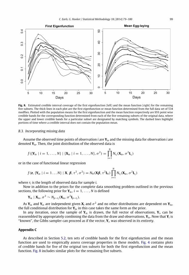
Here we use a ‘‘simulation’’ study to show that credible bands determined through the posteriorsamples provide approximately correct coverage. If we assume the population consists of the originaldata set of 534 flies, the 95% credible bands for the first eigenfunction determined from each of the10 samples from this population ideally contain the population estimate of this eigenfunction 95% ofthe time. While estimating credible interval coverage from ten samples is a very rough measure ofactual coverage, these 10 samples do give us some indication of credible interval behavior. In Figs. 4and 8, credible interval bands for each of the ten samples have been plotted with the populationestimate for the first eigenfunction. Of the ten 95% credible bands, all contain the estimated populationeigenfunction except for the third sample where approximately 25% of the point-wise credible banddoes not include the population estimate. So, roughly, for these ten samples, 97.5% of the credibleintervals include the population estimate of the first eigenfunction. Thus, considering the small samplesize, the empirical coverage of these credible intervals seems to be reasonable.
A similar analysis can be performed for the estimated mean function. Here, however, we comparethe credible interval coverage under our model to the credible intervals obtained by fixing thecovariance function in the GP model in advance instead of estimating it through the Gibbs sampler.This provides a comparison of our modeling approach to methods similar to those of Crainiceanu andGoldsmith [4]. Theoretically, we would expect inference methods that do not account for uncertaintyin the estimate of the covariance function to underestimate variability in parameter estimatesthroughout the model. Our empirical analysis supports this theory.
For the estimates where the covariance function is modeled as known, the covariance functionis fixed at the posterior sample mean of the covariance function from a previous run of the fullGP model for that sample. Consequently, these estimates by definition reflect the best estimatesfor the covariance function for this model and a priori incorporate prior information and data.Since we utilize covariance function estimates from the full model as our ‘‘fixed’’ estimates, in thefollowing analysis, the primary difference between the two models used for each sample is that
92 C. Earls, G. Hooker / Statistical Methodology 18 (2014) 79–100
Fig. 4. Estimated credible interval coverage of the first eigenfunction (left) and themean function (right). The thick lines in eachplot is the first eigenfunction or mean function determined from the full data set of 534 medflies. Plotted with the populationmeans for the first eigenfunction and the mean function respectively are 95% point wise credible bands for the correspondingfunction determined from each of five subsets of the original data, where the upper and lower credible bands for a particularsubset are designated by matching symbols. The dashed lines highlight portions of time where a credible interval does notcontain the population mean. Similar plots for the remaining 5 subsets of data can be found in Appendix C.
in one the covariance function is considered stochastic and in the other the covariance functionis considered known. As can be seen in Figs. 4 and 8, in the GP model where the covariancefunction is stochastic, the credible bands approximately cover the population mean 93% of thetime. However, in the models where the covariance function has been held fixed, the resultingunderestimation of variability is reflected in credible intervals that provide less coverage. Fig. 5presents a comparison of credible bands derived under the two different methods for four samples.Universally, the fixed covariance approach produces narrower credible intervals; over all ten samplesthey cover the population mean estimate 82% of the time. Hence, empirically, there is evidencecredible bands obtainedunder amethodwhere the covariance function or eigenfunctions are assumedknown, but have actually been estimated prior to the inference procedure, do not provide adequatecoverage.
5.3. Missing data results
One advantage of modeling missing data as latent parameters is that the resulting estimates ofa latent function, at time points with missing observations, draw on information from the mean andcovariance processes at those time pointswhile also taking into account the smoothness of the processand neighboring observations. Here we will examine the effect of missing data under two scenarios.In the first, each function is missing blocks of data placed at random along the function. Here theremaining functions continue to provide information about the mean and covariance parameters. Inthe second scenario, the same blocks of data are missing for all functions, forcing our methods to relyon smoothing information to interpolate across the block.
Using sample one, observations are eliminated from the egg-laying data either consistentlythroughout the sample or in blocks of five adjacent observations, where the placement of the fiveobservations varies from curve to curve.Where observations are systematically deleted from the data,all observations from days 9 through 14, 23 through 25, and day 29 are omitted.
The effect of missing observations is seen in the estimates of individual egg-laying trajectories. Asshown in Fig. 7, where the same blocks of data are omitted in every curve, functional estimates differimportantly from their corresponding complete data estimates. This is not surprising as the estimate
C. Earls, G. Hooker / Statistical Methodology 18 (2014) 79–100 93
Fig. 5. Comparison of credible band coverage under fixed and random covariance assumptions. The population mean functionplotted with credible bands for each of four samples under fixed and stochastic covariance assumptions.
Fig. 6. Results for a range of smoothing parameters. These plots highlight the sensitivity of parameter estimates to the choiceof smoothing parameters. The solid lines are estimates with smoothing parameters chosen by the sampler.
94 C. Earls, G. Hooker / Statistical Methodology 18 (2014) 79–100
Fig. 7. Function estimates using incomplete data. Each plot contains three estimates of latent functions from sample one. Thesolid lines are complete data estimates. The dashed lines represent estimates with data missing randomly in blocks. The dottedlines are estimates with data missing consistently in every observation at the time points corresponding to the shaded areas.
of a latent function in areas where no data are available relies only on the smoothing informationin the prior distribution and neighboring estimates of the latent function at observed time points. Incontrast, trajectory estimates determined on the data set with random blocks of missing data lookfairly similar to those estimated using the complete data. The close adherence of curves estimatedwith complete data to curves estimated with random deletions demonstrates how accurately thismodel estimates sections of missing data by using information from supporting curves that includeobservations at these time points.
6. Discussion
For the models described in this paper, the underlying assumption of smoothness in the latentfunctions allows us to move from a finite Gaussian distribution to a Gaussian process. Under thisassumption, just a few actual observations of the process are necessary to elicit important informationabout the entire process. In particular, these assumptions allow for describing the process in terms ofthe posterior distributions of its mean and covariance functions.
In practice, the functional data desired for inference are often latent processes where noisy datarepresenting the underlying processes are observed at a discrete set of time points. The models wepropose here are designed to provide a structure from which more complex models can be built inwhich the data, predictors, or parameters can be modeled as latent Gaussian processes. These include
C. Earls, G. Hooker / Statistical Methodology 18 (2014) 79–100 95
models with latent functional parameters or predictors and models that include functional randomeffects.
These models offer a unified approach to smoothing that takes into account all data and latentparameters and provides model stability. The smoothing parameters can be individualized to eachfunction of interest, and the selection process does not require searching over a range of smoothingparameters or cross-validation procedures.
In this paper, all smoothing parameters and variance components are assigned noninformativeinverse Gamma or Gamma prior distributions. While these distributions have been traditionally usedas conditionally conjugate priors for variance (or inverse variance) components, Gelman [6] has shownthat inmodelswhere the variance componentsmaybe close to zero, or forwhich little data is available,an inverse Gamma prior cannot be considered noninformative. In our examples, we have sufficientdata so that variance components not close to zero (such as the error variance components, σ 2 andτ 2) are largely unaffected by using a ‘‘noninformative’’ inverse Gamma prior. Furthermore, while it ispossible that the smoothing penalties may be small, significant changes to smoothing would requirethese estimates to be off by at least a factor of ten. In his paper, Gelman recommends using a weaklyinformative uniform prior distribution for the square root of a variance component which results inan improper conditionally conjugate prior distribution for the variance component itself. Substitutinguniform priors on the square root of the variance components for the inverse Gamma priors in thesemodelswhen there is only a small amount of data orwhen the variance component is likely to be closeto zero may yield significantly better estimates. See Gelman’s paper for details and for other possiblechoices of prior distributions.
If functional data is to be widely considered for analysis, models are required that are easilyunderstood, and have associated inference procedures that can be easily implemented. The modelspresented here provide for a great deal of flexibility in assumptions and data requirements, andthe ease in which they can be implemented make them attractive for many practical situations. Inthis paper, we have utilized a simple Gibbs sampler to construct samples from the joint posteriordistribution of all unknown parameters. While we have shown in a simulation analysis that theposterior samples obtained through the Gibbs sampler provide accurate parameter estimates, othersampling schemesmay improvemixing and reduce computational cost in thesemodels. Further,morecomplex, nonlinear models incorporating latent functional processes will require the developmentof new, efficient sampling techniques. In particular, recent work by Calderhead et al. [3] suggeststhat population MCMC can be employed to allow both global and local movement throughout theparameter space for a more efficient sampler. A general discussion of adaptive Gibbs samplers andtheir convergence properties can be found in Latuszyński et al. [10].
Acknowledgments
This research was partially supported from NSF grants DEB-0813743, CMG-0934735 and DMS-1053252.
Appendix A
The expected draw of λ(m+1)1 is determined using the full-conditional distribution for λ1 given in
Appendix B. In (10),6−1(m+1)X has been replaced by its expectation in order to examine the relationship
between a new draw of the smoothing parameter and the previous draw of this parameter. The full-conditional distribution fromwhich this expectation has been derived can be found in Appendix B.Wewill assume for this exhibition that the hyperparameters, a and b, associated with the inverse Gammaprior defined for λ1 are sufficiently small that they can effectively be ignored.
E(λ(m+1)1 ) =
tr(P26−1(m+1)X )
(p + 1)(p − 2) − 2
≈tr(P2E(6
−1(m+1)X ))
(p + 1)(p − 2) − 2(10)
96 C. Earls, G. Hooker / Statistical Methodology 18 (2014) 79–100
=
(p + 1 + N)tr
P2
η
−1(m)1 P1 + λ
−1(m)1 P2 +
Ni=1
(Xi − µ)(Xi − µ)′−1
(p + 1)(p − 2) − 2
=
(p + 1 + N)tr
pj=3
κ−1j νjν
′
j
2j=1
η(m)1
1+η(m)1
Ni=1
c2(m)ij
νjν′
j +p
j=3
λ(m)1 κj
1+λ(m)1 κj
Ni=1
c2(m)ij
νjν′
j
(p + 1)(p − 2) − 2
=
(p + 1 + N)tr
pj=3
λ(m)1
1+λ(m)1 κj
Ni=1
c2(m)ij
νjν′
j
(p + 1)(p − 2) − 2
≈ λ(m)1
p + 1 + N
p + 1
1
p − 2
pj=3
1
1 + λ(m)1 κj
Ni=1
c2(m)ij
. (11)
Here, {νj : j = 1 . . . p} are the eigenvectors of the inverse scale matrix, η1P−
1 +λ1P−
2 , where ν1 andν2 penalize linear and constant variation while {νj : j = 3 . . . p} penalize curvature. {η1, η1, {λ1κj :
j = 3 . . . p}} are the corresponding eigenvalues of the inverse scale matrix. Furthermore, for eachj,N
i=1 c2(m)ij represents the variation present in the latent functions in the jth direction in iteration
m that is determined by representing each centered approximation to a latent function as a linearcombination of the eigenvectors of the penalty matrix. The approximation in (11) is due to the
omission of a factor of1 −
2(p+1)(p−2)
−1.
Appendix B
Below, in detail, are the joint data distributions, prior distributions, and full conditionaldistributions for the models discussed in this paper. The first section describes the basic model forsmoothing, estimating, and characterizing latent functional data. The next section expands thismodelto encompass functional linear regression. The third section looks at how to adjust the Gibbs samplerto account for missing observations.
B.1. Estimating latent functional data
As discussed in Section 2, the initial assumption of this model is that we are interested in thefunctional data, Xi(t), i = 1, . . . ,N , modeled by a Gaussian process, for which we only have noisyobservations of each function at a given set of time points, tj, j = 1, . . . , p. Observations, Yi(tj), i =
1, . . . ,N, j = 1, . . . , p, are independent gaussian random variables centered at the value of the latentfunction Xi(t) at time tj with variance σ 2. Thus each observation has distribution
f (Yi(tj) | Xi(tj), σ 2)=N(Xi(tj), σ 2) for i = 1, . . . ,N j = 1, . . . , p
which results in the joint distribution of all observations
f (Y | X, σ 2)=
Ni=1
Np(Xi, σ2I)
where Y is the matrix such that the observation for function Xi(t) at time point tj is in the ith rowand the jth column, X is the matrix of the corresponding means for each entry in Y, and Xi =
(Xi(t1), . . . , Xi(tp))′, the vector of evaluations of the functions Xi(t) at time points t = (t1, . . . , tp)′.
C. Earls, G. Hooker / Statistical Methodology 18 (2014) 79–100 97
The following priors are assumed
Xi | µ, 6X ∼ Np(µ, 6X ) for i = 1, . . . ,Nµ ∼ Np(0, 6µ)
6X ∼ IW (PX , δ)
σ 2∼ IG(a, b)
η1 ∼ IG(a, b) η2 ∼ G(c, d)λ1 ∼ IG(a, b) λ2 ∼ G(c, d)
where a, b, c , and d are fixed hyperparameters and 6µ and PX are hyperparameters that includesmoothing information from the penalty matrix.
In the priors above, the roughness penalties for the latent and mean functions are specificallydefined as (where P1 and P2 are defined in (4)):
PX = η−11 P1 + λ−1
1 P2 and 6µ = η−12 P1 + λ−1
2 P2.
Using these assumptions, the following full conditional distributions are derived to run a MCMCGibbs sampler, for i = 1 . . .N ,
The model above can easily be extended to the framework of a functional linear regression model.With a scalar response, zi and functional predictor Xi(t), we are interested in finding a function β(t)such that
zi = α +
β(t)Xi(t)dt + ϵi, i = 1, . . . ,N
ϵi ∼ N(0, τ 2).
Again, the underlying assumption is that we observe noisy finite dimensional observations of thepredictor Xi(t) such that the distribution of the observations, Yi(tj) is
f (Yi(tj) | Xi(tj), σ 2) ∼ N(Xi(tj), σ 2) for i = 1, . . . ,N j = 1, . . . , p.
Using a finite approximation of the predictor, Xi(t), let X equal the N x (p+1)matrix of predictors,i = 1, . . . ,N where the first column is a column of ones and columns 2 through j + 1 consist ofevaluations of Xi(t) at tj, j = 1, . . . , p. In accordance, we will consider the (p + 1) x 1 vector β suchthat β = (α, β(t1), β(t2), . . . , β(tj))′, a finite approximation of the functional regression coefficient
98 C. Earls, G. Hooker / Statistical Methodology 18 (2014) 79–100
such that α +
β(t)Xi(t)dt ≈ X[i, ]β, for each i = 1, . . . ,N . Under these assumptions the jointdistribution of the independent observations, z = (z1, . . . , zN)′ and the N x pmatrix Y is
The hyperparameters ξ 2, a, b, c , and d are fixed and 6µ, PX and Pβ are hyperparameters thatinclude smoothing information from the penalty matrix. 6µ and PX are as defined in the section onestimating latent functions. Here, we have assumed for simplicity that P−1
β = λ36−1µ . However, if a
separate smoothing parameter for each element of the penalty matrix for the prior on β is desired,the additional smoothing parameter can easily be incorporated into this model.
For i = 1, . . . ,N , define
βX = β[2 : (p + 1)] and 6Xi|rest = (τ−2βXβ′
X + σ−2Ip + Σ−1X )−1.
Then the full conditional distributions for the Gibbs Sampler are:
C. Earls, G. Hooker / Statistical Methodology 18 (2014) 79–100 99
Fig. 8. Estimated credible interval coverage of the first eigenfunction (left) and the mean function (right) for the remainingfive subsets. The thick lines in each plot are the first eigenfunction or mean function determined from the full data set of 534medflies. Plotted with the population means for the first eigenfunction and the mean function respectively are 95% point wisecredible bands for the corresponding function determined from each of the five remaining subsets of the original data, wherethe upper and lower credible bands for a particular subset are designated by matching symbols. The dashed lines highlightportions of time where a credible interval does not contain the population mean.
B.3. Incorporating missing data
Assume the observed time points of observation i are Yio and the missing data for observation i aredenoted Yiu. Then, the joint distribution of the observed data is
f ({Yio | i = 1, . . . ,N} | {Xio | i = 1, . . . ,N}, σ 2) =
where ri is the length of observed data for sample i.Now in addition to the priors for the complete data smoothing problem outlined in the previous
sections, the following prior for Yiu, i = 1, . . . ,N is defined
Yiu | Xiu, σ2
∼ Np−ri(Xiu, σ2Ip−ri).
As Yiu and Yio are independent given Xi and σ 2 and no other distributions are dependent on Yiu,the full conditional distribution for Yiu in this case takes the same form as the prior.
In any iteration, once the sample of Yiu is drawn, the full vector of observations, Yi, can bereassembled by appropriately combining the data from the draw and observations, Yio. Now that Yi is‘‘known’’, the Gibbs sampler can proceed as if the vector, Yi, was observed in its entirety.
Appendix C
As described in Section 5.2, ten sets of credible bands for the first eigenfunction and the meanfunction are used to empirically assess coverage properties in these models. Fig. 4 contains plotsof credible bands for five of the original ten subsets for both the first eigenfunction and the meanfunction. Fig. 8 includes similar plots for the remaining five subsets.
100 C. Earls, G. Hooker / Statistical Methodology 18 (2014) 79–100
References
[1] S. Behseta, R. Kass, G. Wallstrom, Hierarchical models for assessing variability among functions, Biometrika 92 (2) (2005)419–434.
[2] T. Cai, M. Yuan, Nonparametric Covariance Function Estimation for Functional and Longitudinal Data. Technical Report,2010.
[3] B. Calderhead, M. Girolami, N. Lawrence, Accelerating Bayesian inference over nonlinear differential equations withGaussian processes, Advances in Neural Information Processing Systems 21 (2009) 217–224.
[4] C. Crainiceanu, J. Goldsmith, Bayesian functional data analysis using WinBUGS, Journal of Statistical Software 32 (1–33)(2010) 835–837.
[5] A.P. Dawid, Matrix-variate distribution theory: notational considerations and a Bayesian application, Biometrika 68 (1)(1981) 265–274.
[6] A. Gelman, Prior distributions for variance parameters in hierarchical models (comment on article by Browne and Draper),Bayesian Analysis 1 (3) (2006) 515–534.
[7] J. Goldsmith, J. Bobb, C. Crainiceanu, B. Caffo, D. Reich, Penalized functional regression, Journal of Computational andGraphical Statistics 20 (4) (2010) 830–851.
[8] G. Kauermann, M. Wegener, Functional variance estimation using penalized splines with principal component analysis,Stat. Comput. 21 (2) (2009) 159–171.
[9] C. Kaufman, S. Sain, Bayesian functional ANOVA modeling using Gaussian process prior distributions, Bayesian Analysis 5(1) (2010) 123–150.
[10] K. Latuszyński, G. Roberts, J. Rosenthal, Adaptive Gibbs samplers and related MCMC methods, 2011. Arxiv preprintarXiv:1101.5838.
[11] A. Linde, Reduced rank regression models with latent variables in Bayesian functional data analysis, Bayesian Analysis 6(1) (2011) 77–126.
[12] H.G. Müller, U. Stadtmüller, Generalized functional linear models, Ann. Statist. 33 (2) (2005) 774–805.[13] X. Nguyen, A.E. Gelfand, The dirichlet labeling process for clustering functional data, Statistica Sinica 21 (2011) 1249–1289.[14] J. Ramsay, B. Silverman, Applied Functional Data Analysis, Springer-Verlag, New York, 2005.[15] J. Silverstein, The smallest eigenvalue of a large dimensional Wishart matrix, Ann. Probab. 13 (4) (1985) 1364–1368.[16] G. Wahba, Spline Models for Observational Data, Society for Industrial and Applied Mathematics, 1992.[17] S. Wood, Fast stable restricted maximum likelihood and marginal likelihood estimation of semiparametric generalized
linear models, Journal of the Royal Statistical Society 73 (1) (2011) 3–36.[18] F. Yao, H.G. Müller, J.L. Wang, Functional data analysis for sparse longitudinal data, J. Amer. Statist. Assoc. 100 (470) (2005)


![[7] Gaussian Elimination - Coding The ?· Gaussian Elimination [7] Gaussian Elimination. Starting to…](https://static.documents.pub/doc/80x56/5ba1840309d3f2bb6a8c8421/7-gaussian-elimination-coding-the-gaussian-elimination-7-gaussian-elimination.jpg)


