Bayesian Decision Analysis: Principles and Practice Jim Q. Smith J.Q.Smith, Department of Statistics,, University of Warwick, Coven- try CV4 7AL UK E-mail address : [email protected]Dedicated to Pam, Sam and Chris.
The Author thanks to Je¤ Harrison, Bob Oliver, Phil Dawid and Simon French .
Abstract. Replace this text with your own abstract.
Contents
Preface vii
Part 1. Foundations of Decision Modeling 1
Chapter 1. Introduction 31. Getting Started 82. A Simple Framework for Decision Making 93. Bayes Rule in Court 194. Models with Contingent Decisions 225. Summary 236. Exercises 23
Chapter 2. Explanations of Processes and Trees 251. Introduction 252. Using trees to explain how situations might develop 263. Decision Trees 304. Some Practical Issues� 365. Backward Induction Decision trees 406. Normal Form Trees 467. Temporal coherence and episodic trees� 498. Summary 509. Exercises 51
Chapter 3. Utilities and Rewards 531. Introduction 532. Utility and the Value of a Consequence 543. Properties and Illustrations of Rational Choice 664. Eliciting a utility function with a dimensional attribute 705. The Expected Value of Perfect Information 726. Bayes Decisions when Reward Distributions are Continuous 737. Calculating Expected losses 748. Bayes Decisions under Con�ict� 779. Summary 8310. Exercises 84
Chapter 4. Subjective Probability and its Elicitation 871. De�ning Subjective Probabilities 872. On Formal De�nitions of Subjective Probabilities 913. Improving the assessment of prior information 954. Calibration and successful probability predictions 101
Chapter 5. Bayesian Inference for Decision Analysis 1131. Introduction 1132. The Basics of Bayesian Inference 1143. Prior to Posterior analyses 1174. Distributions which are closed under sampling 1205. Posterior Densities for Absolutely Continuous Parameters 1216. Some Standard Inferences using Conjugate Families 1257. Non-Conjugate Inference� 1308. Discrete mixtures and Model Selection 1329. How a Decision Analysis can use Bayesian Inferences� 13510. Summary 13911. Exercises 139
Part 2. Multi-dimensional Decision Modeling 143
Chapter 6. Multiattribute Utility Theory 1451. Introduction 1452. Utility Independence 1463. Some General Characterization Results 1524. Eliciting a utility function 1535. Value Independent Attributes 1556. Decision Conferencing and Utility Elicitation 1607. Real Time Support within Decision Processes 1668. Summary 1689. Exercises 169
Chapter 7. Bayesian Networks 1731. Introduction 1732. Relevance, Informativeness and Independence 1743. Bayesian Networks and DAG�s 1784. Eliciting a Bayesian Network: A Protocol 1885. E¢ cient Storage on Bayesian Networks 1946. Junction Trees and Probability Propagation 1997. Bayesian Networks and other Graphs 2068. Summary 2099. Exercises 209
Chapter 8. Graphs, Decisions and Causality 2131. In�uence Diagrams 2132. Controlled Causation 2243. DAGS and Causality 2274. Time Series Models* 2375. Summary 2396. Exercises 240
Chapter 9. Multidimensional Learning 243
CONTENTS v
1. Introduction 2432. Separation, Orthogonality and Independence 2463. Estimating Probabilities on Trees� 2514. Estimating Probabilities in Bayesian Networks 2565. Technical issues about structured learning� 2606. Robustness of Inference given Copious Data� 2647. Summary 2698. Exercises 270
Chapter 10. Conclusions 2751. A Summary of what has been demonstrated above. 2752. Other types of decision analyses 276
Bibliography 279
Preface
This book introduces the principles of Bayesian Decision Analysis and describeshow this theory can be applied to a wide range of decision problems. It is writtenin two parts. The �rst presents what I consider to be the most important principlesand good practice in mostly simple settings. The second part shows how the es-tablished methodology can be extended so that it can address the sometimes verycomplex and data rich structures a decision maker might face. It will serve as acourse book for a 30 lecture course on Bayesian decision modelling given to �nalyear undergraduates with a mathematical core to their degree programme and sta-tistics masters students at Warwick University. Complementary material given intwo parallel courses one, on Bayesian numerical methods and the other on BayesianTime Series is largely omitted although links to these areas are given within thetext. .It contains foundational material on the subjective probability theory andmultiattribute utility theory - with a detailed discussion of e¢ cacy of various as-sumptions underlying these constructs - quite an extensive treatment of frameworkslike event and decision trees, Bayesian Networks, as well as In�uence Diagrams andCausal Bayesian Networks that help draw di¤erent aspects of a decision probleminto a coherent whole and material on how data can be used to support a Bayesiandecision analysis.
The book presents all the material given on this course. However it also providesadditional material to help the student develop a more profound understandingof this fascinating and highly cross-disciplinary subject. First it includes manymore worked examples than can be given in a such a short programme. Second Ihave supplemented this material with extensive practical tips gleaned from my ownexperiences which I hope will help equip the budding decision analyst. Third thereare supplementary technical discussions about when and why a Bayesian decisionanalysis is appropriate. Most of this supplementary material is drawn from variouspostgraduate and industrial training courses I have taught. However all the materialin the book should be accessible and of interest to a �nal year maths undergraduatestudent. I hope the addition of this supplementary material will make the bookinteresting to practitioners who have reasonable skills in mathematics and helpthem hone their decision analytic skills.
The book contains an unusually large number of running examples which aredrawn - albeit in a simpli�ed form - from my experiences as an applied Bayesianmodeler and used to illustrate theoretical and methodological issues presented in itscore. There are many exercises throughout the book that enable the student to testher understanding. As far as possible I have tried to keep technical mathematicaldetails in the background whilst respecting the intrinsic rigour behind the argu-ments I use. So the text does not require advanced course in stochastic processes,measure theory or probability theory as a prerequisite.
vii
viii PREFACE
Many of the illustrations are based round simple �nite discrete decision prob-lems. I hope in this way to have made the book accessible to a wider audienceMoreover, despite keeping the core of the text as nontechnical as possible, I havetried to leave enough hooks in the text so that the advanced mathematician canmake these connections through pertinent references to more technical material.Over the last twenty years many excellent books have appeared about BayesianMethodology and Decision Analysis. This has allowed me to move quickly overcertain more technical material and concentrate more on how and when these tech-niques can be drawn together Of course some important topics have been less fullyaddressed in these texts. When this has happened I have �lled these gaps here.
Obviously many people have in�uenced the content of the book and I am ablehere only to thank a few. I learned much of this material from conversations withJe¤ Harrison, Tom Leonard, Tony O�Hagan, Chris Zeeman, Dennis Lindley, LarryPhillips, Bob Oliver, Morris De Groot, Jay Kadane, Howard Rai¤a, Phil Dawid,Michael Goldstein, Mike West, Simon French, Saul Jacka, Ste¤en Lauritzen andmore recently with Roger Cooke, Tim Bedford, Joe Eaton, Glen Shafer, MilanStudeny, Henry Wynn, Eva Riccomagno, David Cox, Nanny Wermuth, ThomasRichardson, Michael Pearlman, Eva Riccomagno, Lorraine Dodd, Elke Thonnes,Mark Steel, Gareth Roberts, Jon Warren, Jim Gri¢ n, Fabio Rigat and Bob Cow-ell. Postdoctoral fellows who were instrumental in jointly developing many of thetechniques described in this book include Alvaro Faria, Ra¤aella Settimi, NadiaPapamichail, David Ranyard, Roberto Puch, Jon Croft, Paul Anderson and PeterThwaites. Of course my university colleagues and especially my PhD students, DickGathercole, Simon Young, Duncan Atwell, Catriona Queen, Crispin Allard, NickBisson, Gwen Tanner, Ali Gargoum, Antonio Santos, Lilliana Figueroa, Ana MariMadrigal, Ali Daneshkhah, John Arthur, Siliva Liverani, Guy Freeman and PiotrZwirnick have all helped inform and hone this material. My thanks go out to thesereseasrchers and the countless others who have helped me directly and indirectly.
Part 1
Foundations of Decision Modeling
CHAPTER 1
Introduction
0.1. Prerequisites and notation. This book will assume that the reader hasa familiarly with an undergraduate mathematical course covering discrete probabil-ity theory and a �rst statistics course including the study of inference for continuousrandom variables. I will also assume a knowledge of basic mathematical proof andnotation.
All observable random variables, that is all random variables whose valuescould at some point in the future be discovered, will be denoted by an upper caseRoman letter (e.g. X) and its corresponding value by a lower case letter (e.g.x).In Bayesian inference parameters - which are usually not directly observable - arealso random variables. I will use the common abuse of notation here and denoteboth the random variable and its value by a lower case Greek letter: e.g. �. Thisis not ideal but will allow me to reserve the upper case Greek symbols (e.g. �)for the range of values a parameter can take. All vectors will be row vectors anddenoted by bold symbols and matrices by upper case Roman symbols. I will use= to symbolize a deduced equality and denote that a new quantity or variable isbeing de�ned as equal to something via the symbol ,.
0.2. Bayesian decision analyses and the scope of this book. This bookis about Bayesian decision analysis. Bayesian decision analysis seriously intersectswith Bayesian inference but the two disciplines are distinct. A Bayesian inferentialmodel represents the structure of a domain and its uncertainties in terms of a singleprobability model. In a well built Bayesian model logical argument, science, expertjudgements and evidence - for example given in terms of well designed experimentsand surveys - are all used to support this probability distribution. In their mosttheoretical forms these probability models simply purport to explain observed sci-enti�c phenomena or social behaviour. In their more applied settings it is envisagedthat the analyses can be structured as a probabilistic expert system for possibleused in the support decision processes whose precise details are currently unknownto the experts designing the system.
In contrast a Bayesian decision analysis is focused on solving a given problem orclass of problems. It is of course important for a decision maker (DM) to take dueregard of the expert judgements, current science and respected theories and evidencethat might be summarised within a probabilistic expert system. However she needsto apply such domain knowledge to the actual problem she faces. She will usuallyonly need to use a small subset of the expert information available. She thereforeneeds not only to draw on that small subset of the expert information that isrelevant to her problem at hand - augmenting and complementing this as necessarywith other context speci�c information but also to use this probabilistic informationto help her make the best decision she can on the basis of the information available
3
4 1. INTRODUCTION
to her. When modelling for inference it is not unusual to conclude that there is notenough information to construct a model. But this will not usually be an optionfor a DM. She will normally have to make do with whatever information she doeshave and work with this in an intelligent way to make the best decision she can inthe circumstances.
The Bayesian decision analyses described in this book provide a frameworkthat:
(1) is based on a formalism accommodating beliefs and preferences as theseimpact on the decision making process in a logical way,
(2) draws together sometimes diverse sources of evidence, generally acknowl-edged facts, underlying best science and the di¤erent objectives relevantto the analysis into a single coherent description of her given problem,
(3) provides a description that explains to a third party the reasons behindthe judgements about the e¢ cacy and limitations of the candidate deci-sions available so that these judgements can be understood, discussed andappraised.
(4) provides a framework where con�ict of evidence and con�ict of objectivescan be expressed and managed appropriately.
The extent to which the foundations of Bayesian decision analysis has beenexplained, examined and criticized is unparalleled amongst its competitors. Asstated in [53, ?] there is simply an enormous literature on this topic it would besimply impossible in a single text to do justice to this. However the level of scrutinyit has attracted over the last 90 years has not only re�ned its application but de�nedits domain of applicability. In Chapters 3, 4 and 6 I will review and develop some ofthis background material justifying the encoding of problems so that uncertaintiesare coded probabilistically and decisions are chosen to maximize expected utility.
I have therefore severely limited the scope of this book and addressed only asubset of settings and problems. This will allow me not only to present what Iconsider to be core material in a logical way but also to outline some importanttechnical material in which I have a particular interest. The scope is outlined below.
(1) I will only discuss the arguments for and against a probabilistic frameworkfor decision modelling. Furthermore, for practical reasons I will arguethroughout the book, for a decision analysis the probabilistic reasoningassumed here is necessarily subjective.
(2) I consider only classes of decision problem where a single or group decisionmaker (DM) must �nd a single agreed rationale for her stated beliefs andpreferences and it is this DM who is responsible for and has the authorityto enact the decisions made. The DM will often take advice from expertsto inform her beliefs. However if she admits an expert�s judgement sheadopts it as her own and is responsible for the judgements expressed in herdecision model. Similarly whilst acknowledging, as appropriate, the needsand aspirations of other stakeholders in the expression of her preferences,the DM will take responsibility for the propriety of any such necessaryaccommodation.
(3) The DM has the time and will to engage in building the type of logical andcoherent framework that gives an honest representation of her problem.The model will support decision making concerning the current problemat hand in the �rst instance. However there will often be the promise
1. INTRODUCTION 5
that many aspects of the architecture and some of the expert judgementsembodied in the model will be relevant to analogous future problems shemight face.
(4) The DM is responsible for explaining the rationale behind her choice ofdecision in a compelling way to an auditor. This auditor, for example, maybe an external regulator, a line manager or strategy team, a stakeholder,the DM herself or some combination of these characters. In this book wewill assume that the auditor�s role is to judge the plausibility of the DM�sreasoning in the light of the evidence and the propriety of the scale andscope of her objectives.
(5) It is acknowledged by all players that the decision model is likely to havea limited shelf life and is intrinsically provisional. The DM simply strivesto present an honest representation of her problem as she sees it at thecurrent time. All accept that in the future her judgements may change inthe light of new science, new surprising information and new imperativesand later adjusted or even discarded for its current or future analogousapplication.
The limited scope of this book allows us to identify various players in thisprocess. There is the DM herself whose role is given above. There is an analystwhich will support her in developing a decision model that can ful�l the tasksabove as adequately as possible. There are domain experts to help her evaluatethe potential e¤ects on the objects of their expertise and enacted decision mighthave. Di¤erent experts may advise on di¤erent aspects of the DM�s problem, butfor simplicity we will assume that there is just one expert informing each domainof expertise. Throughout we will assume that the advice given by an expert willbe no less re�ned than a probability forecast of what he believes will happen as aresult of particular actions the DM might take.
Recent advances in Bayesian methodology has been its ability to support deci-sion making in complex but highly structured domains, rich in expert judgementsand informative but diverse experimental and survey evidence; see for example[24],[172]. Explanations of why this is possible and how illustrations of how thiscan be implemented are presented in the second half of the book. The practicalimplementation of such decision modeling has its challenges. The analyst needsto guide the DM to �rst structure her problem by decomposing it into smallercomponents. Each component in the decomposition can then be linked to possi-bly di¤erent sources of information. The Bayesian formalism can then be used torecompose the problem into a coherent description of the problem at hand. Thisprocess will be explained and illustrated throughout this book.
There are now many such qualitative frameworks developed and currently beingdeveloped, each useful for addressing certain speci�c genre of problems. Perforcein this book I have had to choose a small subset if these frameworks I have foundparticularly practically useful in a wide set of domains I have faced. These are theevent/ decision tree - discussed in Chapter 2 - the Bayesian Network - discussed inChapter 7 - and the in�uence diagram and Causal Bayesian Network discussed inChapter 8.
In most moderate or large scale decision making, the DM not only needs todiscover good decisions and policies but also has to be able to provide reasons forher choice. The more compelling she can make this explanation the more likely it
6 1. INTRODUCTION
will be that she will not be inhibited in making the choices she intends to make. Ifher foundational rationale is accepted - and for the Bayesian one expounded belowthis is increasingly the case - she usually still has to convince a third party thatthe judgements, beliefs and objectives articulated through her decision model areappropriate to the problem she faces.
The frameworks for the decomposition of a problem discussed above are helpfulin this regard because - being qualitative in nature - the judgements they embodyare more likely to be shared by others. Furthermore they enable the DM to draw onany available evidence from statistical experiment and sample surveys, commonlyacknowledged as being well conducted, to support as many quantitative statementsshe makes and use this to embellish and improve her probabilistic judgements.This draws us into an exploration of where Bayesian inference and Bayesian de-cision analysis intersect. In Chapter 5 we review some simple Bayesian analysesthat inform the types of decision modelling discussed in this book. In Chapter9 we discuss this issue further with respect to larger problems where signi�cantdecomposition is necessary.
One di¢ culty the DM faces when trying to combine evidence from di¤erentsources when these pieces of evidence seem to give very di¤erent pictures of whatis happening. When should the DM simply act as if aggregating the informationand when should she choose a decision more supported by one source than an-other? Con�ict can also arise when a problem has two competing objectives whereall decisions open to the DM score well in one objective but not the other or onlyscore moderately in both. When should the DM choose the latter type of policyand compromise and when should she concentrate in attaining high scores in justone objective? The Bayesian paradigm embodies the answers to these questions.Throughout the book I will show how various types of con�ict within a given frame-work is being automatically managed and explained within the Bayesian method-ology in the classes of problem I address.
0.3. The development of Statistics and Decision Analysis. It is usefulto appreciate why there has been such a growth in Bayesian methods in recent years.Some 35 years ago data rich structures were only just beginning to be analysed us-ing Bayesian methods. At that time inference still focused on deductions from datafrom a single (often designed) experiments. The in�uence of the physical scienceson philosophical reasoning - often through the social sciences which were striv-ing to become more "objective" - was dominant and the complexity of inferentialtechniques was bounded by computational constraints. Bayesian modeling was notfashionable for a number of reasons:
(1) If decision making was to be objective then the Bayesian paradigm - basedon subjective prior distributions and preferences represented via a utilityfunction - was a poor starting point.
(2) Many of the top theoretical statisticians focused on problem formulationsbased on the physical and health sciences. This naturally led to the studyof distributions of estimators from single experiments that were well de-signed, likelihood ratio theory, simple estimation, analysis of risk functionsand asymptotic inference for large data sets where distributions could bewell approximated. Many foundational statistics courses in the UK stillhave this emphasis. In such problems where data could often be plausi-bly assumed to be randomly drawn from a sample distribution lying in a
1. INTRODUCTION 7
know parametrised family it was natural to focus inference on the develop-ment of protocols which remotely instructed the experimenter about howto draw inference over di¤erent classes of independent and structurallysimilar experiments. Here the obvious framework for inference was onewhich built on the properties of di¤erent tests and estimators which gaveoutputs that could be shared by any auditor. The framework of Bayesianinference, with its reliance on contextual prior information seemed overlycomplicated and not particularly suited to this task.
(3) The development of stochastic numerical techniques was in its infancy. Sofor most large scale problems, asymptotics were necessary. The commonclaim was that even if you were convinced that a Bayesian analysis shouldbe applied in an ideal world the computations you would need to makewere impossible to enact. You would therefore need to rely on large sampleasymptotics to actually perform inferences. But these were exactly theconditions where frequentist approaches usually worked as well and moresimply than their Bayesian analogues.
The environment had changed radically by the 21st century. In a post modernera it is much more acceptable to acknowledge the role of the observer in the studyof real processes. This acknowledgement is not just common in universities. Manyoutside academia now accept that a decision model needs to have a subjective com-ponent to be a valid framework for an inference: at least in an operational setting.Therefore when implementing an inferential paradigm for decision modelling theargument is moving away from the question of whether subjective elements shouldbe introduced into decision processes on to how it is most appropriate to performthis task. The fact that Bayesian decision theory has attempted to answer thisquestion over the last 90 years has made it a much more established, tested andfamiliar framework than its competitors. Standard Bayesian inference and deci-sion analysis is now an operational reality in a wide range of applications, whereasalternative theories - for example those based on belief functions or fuzzy logic -whilst often providing more �exible representations - are less well developed. Whenlooking for a subjective methodology which can systematically incorporate expertjudgements and preferences the obvious prime candidate to try out �rst is currentlythe Bayesian framework.
Secondly the dominant types of decision problems has begun to shift awayfrom small scale repeating processes to larger scale one o¤ modelling and highdimensional business and phenomenological applications. For example in one ofthe examples in this book we were required to develop a decision support systemfor emergency protocols after the accidental release of radioactivity from a nuclearpower plant. Here models of the functionality and architecture of a given nuclearplant needed to be interfaced with physical models describing the atmospheric pol-lutant the deposition of radioactive waste, its passage into the food chain and intothe respiratory system of humans and models of the medical consequences of dif-ferent types of human behaviour. The planning of countermeasures has to takeaccount not only of health risks and costs but also political implications. In thistype of scenario, data is sparse and often observational and not from designedexperiments. Furthermore direct data based information about many importantfeatures of the problem is simply not available. So expert judgements have to beelicited for at least some components of the problem. Note that to address such
8 1. INTRODUCTION
decision problems using a framework which embeds the plant in a sample space ofsimilar plants appears bizarre. In particular the DM is typically concerned aboutthe probability and extent of a given population adversely a¤ected by the incidentat a given nuclear plant, not features of the distribution of sample space of similarsuch plants: often the given plant and the possible emergency scenario is unique!A Bayesian analysis directly addresses the obvious issue of concern.
Thirdly the culture in which inference is applied is changing. Concurrentlyit is not uncommon for policy and decision making to be driven by stakeholdermeetings where preferences are actively elicited from the DM body and need to beaccommodated into any protocol. The necessity for a statistical model to addressissues contained in the subjectivity of stakeholder preferences embeds naturally intoa subjective inferential framework. Moreover businesses - especially those privatecompanies taking over previously publicly owned utilities - now need to producedocumented inferences supporting future expenditure plans. The company needsto give rational arguments incorporating expert judgements and appropriate objec-tives that will appear plausible and acceptable to an inferential auditor or regulator.Here again subjectivity plays an important role. The most obvious way for a com-pany to address this need is to produce a probabilistic model of their predictionsof expenditure based as far as possible on physical, structural and economics cer-tainties, but supplemented by annotated probabilistic expert judgements where nosuch certainty is possible,the company produces. This auditor can then scrutinisesthis annotated probability model and make her own judgements as to whether shebelieves the explanations about the process and expert judgement are credible.Note here that the auditor cannot be expected to discover whether the company�spresentation is precisely true in some objective sense, but only whether what she isshown appears to be a credible working hypothesis and consistent with known facts.In the jargon of frequentist statistics by following Bayesian methods the companytries to produce a single plausible (massive) probability distribution that forms asimple null hypothesis which an auditor can then test in a way she sees �t!
Fourthly computational developments for the implementation of Bayesian method-ologies has been dramatic over the last 30 years. We are now at a stage where evenfor straightforward modelling problems the Bayesian can usually perform her cal-culations more easily than the non-Bayesian. Routine but �exible analyses can nowbe performed using free software such as Winbugs or R and Bayesian methodologyis often now taught using Bayesian methods (see e.g. [76], [129]). The analysisof high dimensional problems has been led by Bayesians using sophisticated theorydeveloped together with probabilists to enable the approximation of posterior dis-tributions in an enormous variety of previously intractable scenarios provided theyhave enough time. The environment is now capable of supporting models for manycommonly occurring multifaceted contexts and for providing the tools for calculat-ing approximate optimal policies. So the Bayesian modeler can now implement hertrade to support decision analyses that really matter.
1. Getting Started
A decision analysis of the type discussed in this book needs to be customized.A decision analysis often begins by �nding provisional answers to the followingquestions:
2. A SIMPLE FRAMEWORK FOR DECISION MAKING 9
(1) What is the broad speci�cation of the problem faced and its context? Howmight a decision analysis help?
(2) Who is the DM - with the authority to enact and responsible for thee¢ cacy of any chosen policy?
(3) Who will scrutinize the DM�s performance? In particular who will au-dit her assessment of the structure and uncertain features of her prob-lem?(sometimes of course this might be DM herself)?
(4) What are the viable options the DM can choose between?(5) What are the agreed facts and the uncertain features that embody a plau-
sible description of what is happening? In particular what is the scienceand what are the socially accepted theories that inform the process un-derlying the decision process? Is expert advice required on these issuesand if so who should be asked?
(6) What are the features associated with the process on which the decisionor policy impinges that are uncertain? How and to what extent do theseuncertainties impact on the assessed e¢ cacy of a chosen policy? Howcompelling will these judgements be to the auditor? Who knows aboutthis interface?
(7) How are the intrinsic and uncertain features that determine the e¢ cacyof any given policy related to one another? Who can advise on this? Whojudgements can be drawn on?
(8) Where are the sources of information and data that might help reduceuncertainty and support any assertions the DM wants to make to anauditor? How might these sources be supplemented by expedient searchor experimentation?
A Bayesian analyst will facilitate the DM by helping her to build her ownsubjective probability model capturing the nature of uncertainties about features ofthe model which might a¤ect her decision, helping her to annotate with supportingevidence why she chose this particular model of the underlying process. The analystwill proceed to elicit her utility function which will take due regard of the needs ofstakeholders. He will then help the DM in calculating her expected utility associatedwith each decision viable to her. The best decisions will then be identi�ed asthose having the highest expected utility score. These terms will all be formallyde�ned below and the theoretical justi�cation and practical e¢ cacy of followingthis methodology explored throughout this book.
2. A Simple Framework for Decision Making
Bayesian decision analysis developed and has been re�ned over many decadesinto a powerful and practical tool. However to appreciate some of the main aspectsof such analysis it is helpful to begin by discussing the simpler methodologies. Sowe start by discussing problems where the responsible DM receives a single reward- usually a �nancial one - as a result of her chosen act. We will later show thatthese earlier methods are simple special cases of the fully developed theory: it isjust the scope for the e¢ cacious use of these simple methods is, from a practicalperspective, rather restrictive. Subsequently in the book these simple techniqueswill be re�ned and elaborated to produce a broad platform on which to base adecision analysis of many problems of increasing complexity.
10 1. INTRODUCTION
Notation 1. Let D - called the decision space - denote the space of all possibledecisions d that could be chosen by the DM and � the space of all possible outcomesor states of nature �.
In this simple scenario there is a naive way for a DM to analyse a decision prob-lem systematically to discover good and defensible ways of acting. Before she canidentify a good decision she �rst needs to specify given two model descriptors. The�rst quanti�es the consequences of choosing each decision d 2 D for each possibleoutcome � 2 �. The second quanti�es her subjective probability distribution overthe possible outcomes that might occur.
More speci�cally the two descriptors needed are:
(1) A loss function L(d; �) specifying (often in monetary terms) how muchshe will lose if she makes a decision d 2 D and the future outcome is� 2 �. We initially restrict our attention to problems where it is possibleto choose � big enough so that the possible consequences � are describedin su¢ cient detail that L(d; �) is known by DM for all d 2 D and � 2 �:Ideally the values of the function L(d; �) for di¤erent choices of decisionand outcome will be at least plausible to an informed auditor.
(2) A probability mass function p(�) on � 2 � giving the probabilities of thedi¤erent outcomes � or possible states of nature just before we pick ourdecision d. If we have based these probabilities on a rational analysis ofavailable data we call this mass function a posterior mass function. Thisprobability mass function represents the DM�s current uncertainty aboutthe future. This will be her judgement. But if she is not the auditorherself then it will need to be annotated plausibly using facts, science,expert judgements and data summaries.
Note that if the spaces D and � are �nite of respective dimensions r and n thenp(�) is a vector of n probabilities, whilst fL(d; �) : d 2 D; � 2 �g can be speci�edas an m � n matrix all of whose components are real numbers. If both D =fd1; d2; : : : ; drg and � = f�1; �2; : : : �ng are �nite sets then the losses fL(di; �j) =lij : i = 1; 2; : : : r; j = 1; 2; : : : ng can be expressed as a table called a decision tableand shown below.
Note that instead of providing a loss function the DM could equivalently providea payo¤ R(d; �) = �L(d; �): In this book we will move freely between these twoequivalent representations choosing the one with the most natural interpretationfor the problem in question.
One plausible looking strategy for choosing a good decision is to pick a decisionwhose associated expected loss to the DM is minimized. This strategy is the basis ofone of the oldest methodologies of formal decision making. Because of its simplicity
2. A SIMPLE FRAMEWORK FOR DECISION MAKING 11
and its transparency to an auditor it is still widely used in some domains. It willbe shown later that such a methodology is in fact a particular example of a fullBayesian one. It therefore provides a good starting point from which to discussmore sophisticated approaches that are usually needed in practice.
Definition 1. The expected monetary value (EMV) strategy instructs theDM to pick that decision d� 2 D minimising her the expectation of her loss [orequivalently, maximising her expected payo¤ ], this expectation being taken usingDM�s probability mass function over her outcome space �.
To follow such a strategy, the DM chooses d 2 D so as to minimise the function
L(d) =X�2�
L(d; �)p(�)
where L(d) denotes her expected loss or, equivalently, maximises
R(d) =X�2�
R(d; �)p(�)
where R(d) denotes her expected payo¤.
Definition 2. A decision d� 2 D which minimizes L(d) (or equivalently max-imises R(d)) is called a Bayes decision.
Remark 1. As we will see later there are contexts when p(�) may be a functionof d as well as �.
Conisder �rst the simplest possible EMV analysis of a medical centre�s treat-ment policies of a mild medical condition which is not painful and where the doctor- our DM - aims to treat patients so as to minimize the treatment cost. Here thecentre (or her representative doctor) is the responsible DM. An auditor might begovernment health service o¢ cials. Note that this is a speci�c example where acause of interest - here a disease - is observed indirectly through its e¤ects - here asymptom.
Example 1. A patient can have one of two illnesses I = 1; 2 and is observedto exhibit symptom A or not, A. Two treatments d1 and d2 are possible and theassociated costs and probabilities are given below.
Costs I = 1 I = 2d1 100 200d2 400 50
I j A I = 1 I = 2 Mn(A)
A p 1� p �A (1� q) q 1� �
It follows that the expected costs of the two treatments given the existence or not ofa symptom are given by
L(d1jA) = 100P (I = 1jA) + 200P (I = 2jA)= 100p+ 200(1� p) = 50(4� 2p)
L(d2jA) = 400P (I = 1jA) + 50P (I = 2jA)= 400p+ 50(1� p) = 50(1 + 7p)
L(d1jA) = 100P (I = 1jA) + 200P (I = 2jA)= 100(1� q) + 200q = 50(2 + 2q)
L(d2jA) = 400P (I = 1jA) + 50P (I = 2jA)= 400(1� q) + 50q = 50(8� 7q)
12 1. INTRODUCTION
So if using the EMV strategy DM will prefer d1 to d2 if and only if
L(d1j:) < L(d2j:)Thus if a patient exhibits symptom A then the DM will prefer d1 to d2 if and onlyif
50(4� 2p) < 50(1 + 7p), p >1
3
and if symptom A is presented then DM will prefer d1 to d2 if and only if
50(2 + 2q) < 50(8� 7q), q <2
3
Now suppose the DM believes that p = q = 34 , so if A is observed she will choose d1
and if A is observed she will choose d2. The DM might then be interested in howmuch she should expect to spend if she acts optimally. This is discovered simply bysubstituting the appropriate probabilities in the formulae above. Thus
L(d1jA) = 50(4� 2� 34) = 125
L(d2jA) = 50(8� 7� 34) = 187:5
So, since P (A) = � and P (A) = 1� �; under optimal action the amount we expectto spend is
L = 125� + 187:5(1� �) = 187:5� 62:5�
Obviously exactly the same technique can be extended to apply to a problemwhen, for each symptom that might be presented, there are many explanatoryillnesses or conditions n and many treatments t. For each presented symptom, theexpected loss associated with each of the t treatments d can be calculated. In thiscase each expectation will be the sum of n products of a probability of an illnessand an associated cost. The DM can then �nd the Bayes decision for each possiblepresented symptom by simply choosing a treatment with the smallest expected cost.Furthermore, by taking the expectation over symptoms under these optimal costswe obtain the expected per patient cost over the given population, just as she didin the simple example above. So at least in this problem the EMV decision rule iseasy to implement and its rationale is fairly transparent, once the losses and theprobabilities (p; q; �) are given. But where do the probabilities come from?
The answer is they need to come from the DM or from an expert she trusts.She will usually need to be able to provide these as a function of the informationshe has and present her reasoning to an auditor in a compelling way to an auditor.We return to this activity later in the book. However the �rst important pointto emphasise about following the EMV strategy in this way is that, perhaps sur-prisingly, in discrete problems like the one illustrated above, optimal acts are oftenfound to be robust to minor misspeci�cation of the values of the parameters of themodel (here (p; q; �)). Thus in the above the DM only needed to know whether ornot p > 1=3 or q < 2=3 before she could determine how to act. It is not unusualfor only coarse information to be provided - for example the probabilities of illnessgiven symptoms - before DM can determine how to act well. Of course, the coarserthe information needed to justify a certain decision rule as a good one, the easier itis for a DM to convince an auditor that she has acted appropriately. In the exampleabove note that the associated expected costs under optimal acts are linear in p(q).
2. A SIMPLE FRAMEWORK FOR DECISION MAKING 13
In general this type of output of an analysis can be more sensitive to the decisionmaker�s expert judgements, though this is often robust too.
Note that if the probabilities are as given above then the DM needs to calculateonly functions that are linear in the probabilities provided. This makes the wholeanalysis easy to perform, depict and communicate to an auditor. As we scale upthe problem so that the size of m and n are large this linearity remains in thesemote re�ned scenarios.
Finally note that the policy does not only apply to a single patient but toall those presenting. However the more general analysis is provisional and timelimited. Changing environments will inevitably cause the various probabilities todrift in time as will the associated costs, so the values of the thresholds governing theoptimal policy will change. Furthermore in the medium to long term, as alternativetreatments become available new policies which incorporate these new treatmentsmay well become optimal and the nature of the best policy may change. Moreoverthere may well be changes in stakeholder�s needs forcing the decision not just tobe driven by cost but also other factors, for example the speed of recovery of thetreated patient. This again may well change the evaluation of the e¢ cacy eachtreatment policy and provoke changes in the optimal decision.
2.1. Reversing Conditioning. Even in the straightforward context giventhe problem described above is simpli�ed in two ways that make it an unsatifac-tory template for inference in such scenarios. First a doctor will normally observeseveral symptoms, not just one. Second we have noted that probabilities need tobe provided by the DM to make it work. Psychological studies, see Chapter 4, havedemonstrated that probability statements are usually most reliably and robustlyestimated or elicited when conditioned in an order that is consistent with whenthey happened. Here diseases cause symptoms and happen before them. So theanalyst should encourage the DM to specify her joint distribution over diseases andsymptoms via the marginal probability of the cause - here the disease - and theprobability of the e¤ect given a cause: here the probability of the symptom giveneach disease. But in the illustrative example above, to obtain simple expressions,we have speci�ed the inputs to the decision analysis as the symptom margin andthe probability of a disease given a symptom . This is not consist with their causalorder.
Notation 2. Let I denote the disease of the patient with sample space f1; 2; :::; ng;so there are n possible explanatory diseases and m symptoms are observed. De�nethe random variable fYk : 1 � k � mg to be indicators on the m symptoms -i.e. fYk = 1g when the kth symptom is present and fYk = 0g when it is absent,1 � k � m- and write the binary random vector Y = (Y1; Y2; ::; Ym):
Noting the comment on causation in the second bullet above, the informationthe doctor would often employ either from hard data or elicited scienti�c judgementswould usually be about:
� The relative prevalence of the di¤erent possible n diseases as re�ected bythe marginal probabilities of diseases.fP (I = i) : 1 � i � ng. Supportinginformation about these probabilities could be obtained from relevant pre-vious case histories of the population concerned, or failing that be derivedfrom scienti�c judgements about the typical exposures of this population.
14 1. INTRODUCTION
� Scienti�c knowledge about the ways in which a given disease might man-ifest itself through the m observed symptoms. This could be expressedthrough the set of conditional probabilities fP (Y = yjI = i) : y a bi-nary m string, 1 � i � ng. Again support for these probabilities couldcome either from case histories or scienti�c judgements associated witheach possible disease considered: for example the probability the patientexhibited a high temperature given they had a particular disease. Theseissues are addressed in detail in Chapters 4,5 and 9.
Fortunately this type of causally consistent information is enough to give theDM what is needed to perform an EMV analysis. Thus, provided that P (Y = y) >0, i.e. provided there is at least a small chance of seeing the combination ofsymptoms y, when presented by the set of symptoms x; the probabilities fP (I =ijY = y) : 1 � i � ng, can be calculated by simply applying Bayes Rule
(2.1) P (I = ijY = y) =P (Y = yjI = i)P (I = i)Pni=1 P (Y = yjI = i)P (I = i)
Incidentally note that if P (Y = y) = 0 then the doctor would believe she wouldnever see this observation. So in this case there is no need to calculate the corre-sponding posterior probabilities.
We have illustrated above that to assess the expected costs of this action DMneeds fP (Y = y) : y a sequence of 0�s and 1�s of length mg in this population. Butthis is also easy to calculate from these inputs: we use the Law of Total Probabilitywhich tells us that
(2.2) P (Y = y) =nXi=1
P (Y = yjI = i)P (I = i)
Note that these standard equations, whilst familiar to anyone who has studiedan introductory course in probability, are non linear functions of their inputs. Theresults of mapping from
fP (I = i) : 1 � i � ngfP (Y = yjI = i) : y a binary m string; 1 � i � ng
to the corresponding pair
fP (Y = y : y a binary m stringg;fP (I = ijY = y : y a binary m string; 1 � i � ng
can often surprise the DM. Later in this chapter we discuss how this formula canbe explained. But note that because the consequences of these rules have beenexamined exhaustively by probabilists over the last centuries it is relatively easy toconvince an auditor that these are the rules that should be used to map form oneset of belief statements to another. If the DM decides to use an alternative wayof expressing her uncertainty than through probability then the appropriate mapsbetween belief statements have to be justi�able. In practice this is likely to be achallenge.
2.2. Naive Bayes and Conditional Independence. Although Bayes Ruleand the Law of Total Probability can be used to solve the technical problem de-scribed above there remains a serious practical issue to resolve. Thus for each
2. A SIMPLE FRAMEWORK FOR DECISION MAKING 15
disease I = i - because we know that all these probabilities must sum to one -weneed to obtain the 2m � 1 probabilities.
fP (Y = yjI = i) : y a binary vector of length mgEven for moderate values of m this elicitation will be an resource expensive task.Furthermore, because this large number of probabilities they must all be non-negative and sum to one, at least some will be be very small. Experience hasshown that to accurately estimate or elicit probabilities of events which occur withvery small probability is di¢ cult: see Chapter 4. However there are various ac-cepted formulae from probability theory - called credence decompositions - thatcan be used to address the latter practical di¢ culty. One of these is introducedbelow.
To avoid, as far as possible, having to make statements about very small prob-abilities like those above, recall that from the de�nition of a conditional probabilitythen if Y = (Y1; Y2), then
Using this rule but conditioning on fI = ig therefore gives
P (Y = yjI = i) = (mYj=2
P (Yj = yj jY1 = y1; :::; Yj�1 = yj�1; I = i))P (Y1 = y1jI = i)
This is a useful formula because all probabilities in the product on the right handside of this equation are typically much larger than those on the left. This isbecause a product of numbers all of which lie between zero and one is smallerthan any of its components. It follow that the elicitation of these conditionalprobabilities will in practice be more reliable. However, the original problem stillremains. There are still the same large number of probabilities input into thisformula before P (Y = yjI = i) can be calculated. But because we have respectedthe causal order inherent in this problem, it is sometimes appropriate to makea further modeling assumption which helps to circumvent the explosion of theelicitation task.
Definition 3. Symptoms Y = (Y1; Y2; :::; Ym) are said to be conditionallyindependent given the illness I - written qmj=1Yj jI - if for each value of i; 1 � i � n,
(2.3) P (Y = yjI = i) =mYj=1
P (Yj = yj jI = i)
Note that, under this assumption, unlike the general equation above, eachprobability on the right hand side is a function of only two arguments.
Definition 4. The naive Bayes model assumes that all symptoms are inde-pendent given the illness class fI = ig for all possible illness classes i; 1 � i � n.
Although a naive Bayes model embodies strong assumptions, for a variety ofreasons such simple models often work surprisingly well in many applications -including medical ones - and provide a benchmark from which to compare more
16 1. INTRODUCTION
sophisticated models, some of which are discussed later in Chapter 7 and 9. Es-sentially the model asserts that if the disease status of a patient is known thenthe presence or absence of one symptom would not a¤ect the probability of thepresence or absence of a second. So if for example, for a given disease, whenevera patient exhibited the symptom of a high temperature he always also exhibitedthe symptom of nausea, but otherwise there was no connection between the twosymptoms then the naive Bayes model would not be valid.
Note that, when there are n binary symptoms and n diseases in the modelabove, the naive Bayes model needs only mn + n � 1 probabilities to be input,whilst the general model has 2mn� 1. So for example if the doctor observes with 8binary symptoms and 10 possible illnesses, to build this inference engine under thenaive Bayes needs 89 probability inputs, perhaps an afternoon�s elicitation, whereasthe general model needs 2; 559: In general naive Bayes models are therefore muchless expensive to elicit than some of their more sophisticated or general competitors.
2.3. Bayes Learning and Log Odds Ratios. Why does Bayes Rule takethe form it does and how exactly does it work? One of the best ways of explaininghow information from symptoms transforms beliefs is to express this transformationthis is in terms of a function of the illness probabilities - log odds ratios (or scores)Note that odds are commonly used in betting - for example in horse racing gambles- so many people are familiar with the numbers as an expression of uncertainty. Infact some e.g. [257], [158] have advocated the elictation of odds - or their logarithmthe logodds - instead of probability.
Under the Naive Bayes Assumption, provided that P ((Y = y) > 0, i.e. pro-vided that it is not impossible to observe any one of the combination of symptomsx, then
P (I = ijY = y) =P ((Y = yjI = i)P (I = i)
P (Y = y)=
Qmj=1 P (Yj = yj jI = i)P (I = i)
P (Y = y)
and
P (I = kjY = y) =P ((Y = xjI = k)P (I = k)
P (Y = x)=
Qmj=1 P (Yj = xjnI = k)P (I = k)
P (Y = y)
So, provided that P (I = kjY = y) > 0, dividing these two equation gives that
P (I = ijY = y)
P (I = kjY = y)=
mYj=1
�P (Yj = yj jI = i)
P (Yj = yj jI = k)
�:P (I = i)
P (I = k)
which, on taking logs can be written in the linear form
(2.4) O(i; kjy) =mXj=1
�j(i; k; yj) +O(i; k)
where the prior log odds of I are de�ned by
O(i; k) = log
�P (I = i)
P (I = k)
�and the posterior log odds of I are de�ned by
O(i; knx) = log�P (I = ijY = y)
P (I = kjY = y)
�
2. A SIMPLE FRAMEWORK FOR DECISION MAKING 17
and the log �likelihood ratio of the jth observed symptom is given by
�j(i; k; yj) = log
�P (Yj = yj jI = i)
P (Yj = yj jI = k)
�Thus the posterior log odds between i and k are the prior log odds between
these quantities plus a score �j(i; k; xj) re�ecting how much more probable it wasto see the observed symptom yj were I = i rather than I = k. The linearity of therelationship between prior and posterior odds means that the DM can quickly cometo a good appreciation about how and why what she has observed - the symptoms- has changed her odds between two diseases. Note that:
(1) The larger O(i; k), the more probable the DM believes the disease i tobe relative to disease k a priori. In particular when O(i; k) = 0 beforeobserving any symptoms DM believes the diseases i and k to be equallyprobable.
(2) If the probability of the observed symptoms under two illnesses are thesame then this implies that
mXj=1
�j(i; k; yj) = 0
The formula (2.4) therefore tells us that the relative probability of theillnesses a posteriori is the same as it was a priori: a very reasonablededuction! On the other hand an observed symptom yj contributes toan increase in the probability of illness i relative to the probability ofillness k if and only if �j(i; k; yj) > 0. This inequality is equivalent to thestatement
P (Yj = yj jI = i) > P (Yj = yj jI = k)
i.e. when the probability of what we have seen if greater under the hypoth-esis that I = i than I = k then the probability of disease i will increaserelative to the probability of disease k. Again this appears eminentlyreasonable.
(3) More subtly note that �j(i; k; yj) will be very large and have a dominatinge¤ect on O(i; kjy) whenever P (Yj = yj jI = i) is much greater than P (Yj =yxj jI = k), even when P (Yj = yj jI = i) is very small, i.e. even when thesymptom is unlikely for the more supported illness is minute. So unlessthese small probabilities can be elicited accurately - and often this isdi¢ cult - the posterior odds calculated by the formula above may wellmislead both the DM and the auditor. In general Bayes Rule updatingcan be very sensitive to elicited or estimated probabilities when the dataobserved has a small probability under all explanatory causes.
It is straightforward - if rather tedious - to express the posterior probabilitiesas a function of some of the log odds ratios (see Exercise 7) . Thus, after a littlealgebra, it can be shown that
(2.5) P (I = ijY = y) =exp[O(i; 1jy]
[1 +Pn
k=2 exp[O(k; 1jy]]So having calculated O(k; 1jy) 2 � k � n using (2.4) - i.e. the posterior logodds ofthe �rst illness against the rest we can �nd the posterior illness probabilities usingequation (2.5). This formula holds for any labelling of the illness, although it is
18 1. INTRODUCTION
sometimes useful for interpretative purposes to choose the �rst listed illness to bethe simplest or most common one.
Example 2. Suppose the DM believes that there are 3 possible disease I =1; 2; 3; all with equal prior probability. The doctor observes four binary symptomsfSk : 1 � k � 4g in that order. An expert trusted by the DM has judged that theNaive Bayes Model is appropriate in this context and has given the probabilities ofthe the ith symptom being present given the di¤erent illness in the table below
The doctor now observes the �rst three symptoms as present whilst the last as absent.Calculating her posterior odds and hence her probabilities pj(i) after observing the�rst j symptoms using the formulae above it is easily checked that they are given inthe table below
Notice that after the seeing the �rst symptom the probability of the �rst illness is0:5 the highest. This remains the same after the second symptom since what theDM observes is equally probable given all explanations. Therefore this symptom hasno explanatory power. The third symptom lends further support to the �rst illnessbeing the right one, but the absence of the last symptom - an unlikely explanationof any observation for any of the illnesses - reverses the order of the probability,making the �rst illness very unlikely.
This example illustrates the three bullets above. Note in particular that thediagnosis depends heavily on the absence of the last symptom. This has a smallprobability for all the illnesses and a very small probability for the �rst. So thereason for the diagnosis can be fed back to the doctor: that "the unlikely absence ofthe 4th symptom and the relatively better explanation of this observation providedby illness 3 outweighs in strength all other evidence pointing in the other direction".This might be acceptable to the doctor or the external auditor. Alternatively sheor he may question whether the elicited small probabilities of this symptom werepossibly inaccurate or not apposite to this particular patient. A reasoned and sup-ported argument for adjusting these probabilities could then lead to a documentedrevision of the diagnosis.
A second point is that the particular symptoms actually observed from a patientwith illness 3 turn out to be the most unlikely to be observed, being observed onsuch a patient with only the small probability 0:0024. So the reason illness 3has been chosen is that it provides the best of a poor set of explanations of theobserved symptoms. An auditor of the doctor - perhaps the doctor herself! - maywell question why, on this basis, she did not search for a di¤erent explanation. Theinference is only stable if the doctor really does believe that only the three illnessesshe has considered are the only possibilities and the relative odds are really accurate.
Thus for example suppose that a 4th illness with a prior probability of only 0:05as probable as the other alternatives was omitted from consideration in the original
3. BAYES RULE IN COURT 19
analysis for simplicity. Suppose however that under this hypothesis the presence ofthe �rst three symptoms actually observed was very likely - for example > 0:8 - andthe absence of the last symptom was also likely - again with probability > 0:8. Thenit is easy to calculate that this illness would have a posterior probability more than8 times larger than illness 3 provides. Incidentally note that, unlike probabilities,posterior odds of new alternatives like this can be calculated and appended to theoriginal analysis without changing the posterior odds between the earlier calculateddiseases.
So when any explanation of the data is poor this is a cue to feedback thisinformation to the DM. Good Bayesian analyses run with diagnostics that aredesigned to allow an auditor to check whether every model in a given class modelsmight give poor explanations of the evidence. These diagnostics can be designedto inform either the plausibility of the analysis as it applies to the case in hand, oralternatively to the class of problems to which the analyses purport to apply. Theyprompt the DM to creatively reappraise her model.
3. Bayes Rule in Court
3.1. Introduction. Recently, spurred on by the proliferation of DNA evi-dence, various experts have given probabilistic judgements in court about thestrength of evidence supporting a match between the suspect and the crime. Inprinciple at least, the juror�s task is relatively straightforward. This gives an in-teresting new and accessible context for which the type of Bayesian analysis ispertinent.
Jurors - our DM�s in this example - need to assess the probability of guilt (G)or otherwise (G) of the suspect given any background information (B) they havealready been given and the new piece of evidence (E) delivered by the expert. Bylaw, the only persons allowed to make an assessment of the guilt or innocence ofthe suspect is a juror, whether this is before the new evidence arrives (P (GjB)) orthe probability (P (GjB;E)) of guilt in the light of the new information E.
Let us assume that the juror is reasoning logically along the lines we havedescribed above. Then her posterior odds need to be the product of her prior oddsand the likelihood ratio. Thus explicitly she should calculate the odds of guiltover innocence given the background information and the new evidence using theformula
(3.1)P (GjB;E)P (GjB;E)
=P (GjB)P (GjB)
� P (EjG;B)P (EjG;B)
The important implication here is that - to encourage a juror to be rational- the expert should only be allowed to provide jurors with information about thestrength of evidence by communicating - either explicitly or implicitly - the value ofthis likelihood ratio. This is the probability of the actual evidence observed giventhe suspect is guilty relative to the probability of that evidence given the suspect isinnocent - both conditional on the background information B provided to everyone.For example for the expert to present the probability of the evidence given guilt,or given innocence on their own is super�uous and has potential for confusing thejury.
Tables of this formula can be help jurors come to an appropriate revision oftheir beliefs. For example in the table below, prior and posterior log odds of guiltand prior and posterior probabilities of guilt when a credible expert witness asserts
20 1. INTRODUCTION
that the evidence is 100� more probable when the suspect is guilty than when sheis innocent.
3.2. A Hypothetical Case Study. To demonstrate these principles we nowgive a hypothetical study about a typical scenario that might be met in court.Woman A�s �rst child died of an unexplained cause (B). When her second child alsodied of an unexplained cause (E) she was arrested and she was tried for the murderof her two children (hypothesis G). This was the prosecution case. The defensemaintained that both her children died of SIDS (sudden infant death syndrome).An expert witness asserted that only one in 8; 500 children die of SIDS so
P (E;BjG) =�
1
8; 500
�2' 1
73� 106
Apparently the jury treated this �gure as the probability of A�s innocence - i.e.as P (GjE;B). This spurious inversion is sometimes called the prosecutor fallacy.So jury members calculating her probability of guilt as
P (GjE;B) = 1� P (GjE;B)
= 1� 1
73� 106found guilt "beyond reasonable doubt". On the basis of this and other evidencethe jury convicted her for murder and she was sent to prison.
3.2.1. The �rst probabilistic/factual error. It is well known that if a mother�s�rst child dies of SIDS then (tragically) her second child is much more likely todie too. For example it is conclusively attested that a tendency to the conditionis inherited. The conditional independence assumption implicit expert witnesses�calculation is therefore logically false. Suppose on the basis of an extensive surveyof records of such cases that
P (EjB;G) ' 0:1Assuming the �gure above.
P (E;BjG) = P (EjB;G)� P (BjG) l 1
85� 103This is a over 850 times larger than the probability than the one quoted by theexpert.
3.2.2. The second error: the prosecutor fallacy. From the rules of probabilitywe know that, in general,
P (GjE;B) 6= P (E;BjG)To obtain P (GjE;B) the juror must apply the Bayes Rule formula: something
very di¢ cult to do in her head. Note that it is not unreasonable for a statisticallynaive but otherwise intelligent juror to assume that these two probabilities are the
3. BAYES RULE IN COURT 21
same when expressed in words (i.e. "the probability this SIDS event will happento an innocent parent suspect") However for an expert witness who presents theprobability P (E;BjG) as if it is P (GjE;B) is either statistically incompetent orconsciously trying to mislead the jury.
3.2.3. A rational analysis of this issue. This uses the formula 3.1 above. Herewe need the juror�s prior odds of guilt. These are of course dependent on everythingthat juror has heard in court. However suppose that one useful statistic, obtainedby surveying death certi�cates in Britain over recent years, is the following. Ofchildren who die in ways unexplained by medicine, less than 1
11 are subsequentlydiscovered to have been murdered. With no other information taken into accountother than this, a typical juror might set
P (GjB)P (GjB)
� 1
11(10
11)�1 = 0:1
So after learning of the �rst child�s death a juror believing this statistic wouldconclude the probability that the child was murdered by her parents was at least10 times less probable than that there was an innocent explanation of the death.Note that this is consistent with actual policy in the UK where someone like A wholoses a �rst baby for unexplained reasons but for whom there are no other strongreasons to assume she had murdered her baby, is freely allowed to conceive andhave a second child. Surely if it was thought that such a woman probably did killher baby, then at least one would expect that the second child would be taken intocare or into hospital where he could be monitored. So the numbers given abovecould be expected to pass a reasonable auditor as at least plausible.
Logically, guilt as it is de�ned implies that
P (EjG;B) = 1and we are taking
P (EjG;B) = 0:1so equation 3.1 gives us that
P (GjB;E)P (GjB;E)
� 0:1� 1
0:1= 1
, P (GjB;E) � 0:5In the face of this evidence, the suspect should therefore not be seen as guilty
beyond reasonable doubt. Although the value of P (GjB;E) might vary betweenjurors, most rational people substituting di¤erent inputs into the odds ratio formulashould convince themselves that, on the basis simply of the deaths, any convictionwould be unsafe. This activity of investigating the e¤ect of di¤erent plausible valuesof inputs into a Bayesian analysis is sometimes called a sensitivity analysis.
The example provides us with a scenario where a DM legitimately adopts someof the conditional probabilities she needs for her inference from an expert: herethe forensic statistician, in a way likely to be acceptable to any auditor. She thencombines these probabilities that legitimately come from herself to come to a robustand defensible decision.
Why do expert witnesses mislead the jury by providing P (E;BjG) and notprovide the analysis above? One reason is that many of them really don�t under-stand ideas of probability and independence well enough to understand the issuesdiscussed above. Indeed applying the rules of probability appropriately to a given
22 1. INTRODUCTION
scenario is quite hard without help. They therefore mislead themselves as well asthe jury. A second possible reason is that they tend to see the most horrible casesand disproportionately few innocent ones. This selection bias discussed in Chap-ter 4 makes their own assessments of the prior odds of guilt unreasonably high.Their own posterior assessments of guilt are consequently in�ated as well and theygenuinely try and convey these in�ated odds to the jury. But whilst explicable thecommunication of this personal false judgement is clearly counter the principle thatthe jury should decide on the basis of the evidence, not the prejudices of the expert!
Further discussion of this and related problems can be found in [37] and [1].
4. Models with Contingent Decisions
The scenarios illustrated in the last sections have a very straightforward struc-ture. In many decision problems the structure of the model is less obvious. Findingan EMV strategy is then not quite such a transparent task.
Example 3. A laboratory has to test the blood of 2n people for a rare diseasehaving a probability p of appearing in any one individual. The laboratory can eithertest each person�s blood separately [decision d0] or randomly pool the blood of thesubjects into 2n�r groups of size x = 2r , r = 1; 2; :::; n [decision dr] and testeach pooled sample of blood. If a pool gives a negative result then this would meanthat each member of the pool did not have the disease. If the pool gave a positiveresult then at least one member of the pool would have the disease and then all themembers of that pool would then be rechecked individually. Assuming that any test,either pooled or individual, costs £ 1 to perform what is DM�s EMV strategy for thisproblem.
Note that L(d0) = 2n and if the DM decides [dr] to pool into groups of x = 2r
then the probability that this pooled sample is positive is
P (group +ive) = 1� P (group -ive) = 1� (1� p)x , �
Therefore since under dr the number of groups 2n�r = 2nx�1 the expectednumber of pooled samples to recheck is 2n�
x . So the expected number of recheckedindividuals under dr is
x:2n
x� = 2n[1� (1� p)x]
The expected total cost of using decision dr is the number of tests on groupsplus the expected number of rechecked individuals under that regime
where x = 2r; 1 � r � n. For any �xed value of p the expected losses associatedwith dr can be compared.
There are three main points to take away from this example. The �rst is thatif probability distributions of outcomes depend on what the DM decides to do thenfollowing an EMV strategy becomes less transparent unless tools are developed toguide calculations.
The second illustrates the provisional nature of any decision analysis. Thushaving completed this analysis we might reasonably question why we only considerpooling groups of size a power of 2: In fact we could extend the analysis above in astraightforward way to calculate the expected losses associated with other pools of
6. EXERCISES 23
arbitrary group size. If we do this we �nd that the formulae are less elegant to theones above but look very similar and are simple to calculate. More interestingly, ifthe DM decides to pool into a large group and this turns out to be positive, insteadof subsequently then testing all the individuals in the group separately she couldconsider whether to check the further possibility of testing subgroups of this group�rst and only subsequently test individuals in positive subgroups.
Exploring new possibilities of extending the decision space in ways like thosesuggested above is an intrinsic part of a decision analysis. It involves both theDM e.g. "Is it scienti�cally possible to split the blood sample into more thattwo groups and if so how many?" - and the analyst - "Is there some technicalreason why a suggested new decision rule must be suboptimal and therefore notworth investigating". Note that such embellishments of the decision problem donot destroy the original analysis. The original expected losses associated with otherdecisions - and thus their relative e¢ cacy - remain the same no matter how manyalternative decisions we investigate. The earlier analyses of the relative merits ofdecision rules hold �xed, its just we might �nd a new and better one.
Finally note that by developing a structure to address this speci�c problembrings with it an analogous methodology for addressing problems like it. For ex-ample the analysis above applies to the detection of other similar blood conditionsacross other similar populations, albeit with an appropriate change of the probabil-ity p. We will see in many of the problems addressed in this book, it is possible tocarry forward the structure of parts of the problem as well as some of the probabilityassessments. This is one feature that can make a decision analysis so worthwhile:it not only provides support for the decision problem at hand, but also informsanalogous decision analyses that might be performed in the future.
5. Summary
We have seen illustrated above how if a DM is encouraged to choose a decisionminimizing her expected loss then this provides her with a framework that allowsher both to systematically explore her options and develop and examine her be-liefs. This methodology not only helps her make a considered choice but developarguments explaining why she chose the policy she did to an external auditor in alogical and consistent manner. These analyses will also usually inform her decisionmaking about future scenarios whenever these share features with the problem athand.
Even in the very simple examples in this chapter we have been able to demon-strate that the role of the analyst is to support the DM to make wise and defensibledecisions and help her to explore as many scenarios and options as she needs to inorder to have con�dence in her decisions. The analyst�s task is never to tell the DMwhat to do but to provide frameworks to help her creatively explore her problemand to come to a reasoned decision she herself owns as well as providing a templateframework which she might adjust in a decision analysis of similar problems shemight meet in the future.
6. Exercises
1) The e¤ect of d kilograms of fertilizer , 0 < d < 1; 000 on the expected yield� of a crop is given by � = 10(8+
pd). the cost of a kilogram of fertilizer is £ 5 and
the pro�t from a unit of crop is £ 10. Find The EMV decision rule.
24 1. INTRODUCTION
2) Prove the assertion in the text concerning the change in probability followingthe introduction of a 4th explanation of the symptoms in the �rst example onmedical diagnosis.
3) In the example above prove that if p > 1 � 2�1=2 then you should simplyapply d0 whilst otherwise you should �rst pool the blood in some way.
4) In the example above show that d2 is at least as good as d1 for all values ofp so that DM should never pool into groups of 2: groups of 4 being always better.
5) DM is in charge of manufacturing T-shirts in aid of a sponsored marathonrace in 50 week�s time. Leasing a small machine for manufacturing these (decisiond1) will cost £ 100,000 whilst leasing a large machine ( decision d2) will cost £ 300,000over these 50 weeks. DM hopes to obtain free TV advertising with probability p.If this happens she expects to sell 1800 items a week but if not she expects to sellonly 400 a week. If DM makes £ 10 clear pro�t for each T-shirt sold �nd show thather Bayes decision is to to buy the smaller machine if p < 4=13.
6) Items you manufacture are independently �awed with probability � andotherwise perfect. If DM dispatches a �awed item she will lose a customer withan expected cost to him of £A. DM can dispatch the item immediately (d1) orinspect it with a foolproof method, and keep replacing the item and checking untilshe �nds a good one (decision d2). The cost of making an item is £B and the costof checking it £ C
. i) Show that when A = 10; 000, B = 3; 000 and C = 1; 000 under an EMVdecision rule you should prefer d2 to d1 when 0:2 < � < 0:5:
ii) Show that if AB < 4 the DM should never inspect regardless of the value of�:
iiii) Show that the DM should inspect for some value of � if
A2 +B2 > A (C + 2B)
iv) Show that if B = 0 the DM should inspect if and only if � < 1� CA and if
C = 0 if and only if �� � 1
2
�2<1
4� B
A
7) Prove the formula (2.5) above which expresses probabilities in terms of lo-godds.
CHAPTER 2
Explanations of Processes and Trees
1. Introduction
Some simple decision problem can be transparently solved using only descrip-tors like a decision table and some supplementary simple belief structure like naiveBayes model. However for most moderately sized problems the analyst will oftendiscover that the explanation of the underlying process, the consequences and thespace of possible decisions in a problem has a rich and sometimes complex structure.Whilst it is possible to follow an EMV strategy in such domains, the elicitation ofthe description of the whole decision problem is more hazardous. The challenge istherefore to have ways of encapsulating the problem that are transparent enoughfor DM, domain experts and auditors to check the faithfulness of the description ofa problem but which can also be used as a framework for the calculations the DMneeds to make to discover good and defensible policies.
One of the most established encompassing frameworks is a picture, called adecision tree depicting, in an unambiguous way, an explanation of how events mightunfold. Over the years historic trees have been used to convey the sorts of causalrelationships which populate many scienti�c and social theories and hypotheses.These hypotheses about what might happen - represented by the root to leaf pathsof the tree - describe graphically how one situation might lead to another andare often intrinsic to a DM�s understanding of how she might in�uence eventsadvantageously. It is often possible for DM to use this tree to describe, quantifyand then evaluate the consequences of following di¤erent policies. This process willsupport her when she compares the potential advantages and pitfalls of each policyand �nally comes to a plausible and defensible choice of a particular decision rule.Already in Chapter 1 some of the advantages of ordering variables consistentlywith their causal history have been pointed out. In this chapter the elicitationand evaluation tool - the historic tree - is introduced which provides a compellingframework for communicating the input of a decision analysis to an auditor.
We also saw in the last chapter that in order to calculate an optimal policiesit is often expedient to use Bayes Rule to reverse the directionality of conditioningsort is consistent with the order the DM becomes aware of information: for example- in the health diagnosis scenario described there - to condition of symptoms beforeconsidering their causes the diseases. This encourages the analyst to transform ahistoric tree so that it accommodate fast calculation and a transparent taxonomy ofthe space of decision rules rather than transparent explanation. This transformationprocess to a rollback tree is explained and illustrated below.
Another tree especially useful to help the DM and her auditor to become awareof the sensitivity of her analyses to the inputs of her analysis is the normal form tree.In this chapter we will discuss various examples of di¤erent levels of complexity that
25
26 2. EXPLANATIONS OF PROCESSES AND TREES
illustrate how these di¤erent tree structures can be used to represent a problem, bea framework for the calculation of optimal policies and form the basis of a sensitivityanalysis.
2. Using trees to explain how situations might develop
2.1. Drawing historic trees. Throughout this book directed graphs are usedas various frameworks for describing a model. So it is useful to begin this sectionwith some general de�nitions A directed graph G = (V (G); E(G)) is de�ned by a setof vertices denoted by V (G) and a set of directed edges denoted by E(G) connectingthe vertices of the graph to one another. If a vertex v0 2 V (G) is connected by anedge in E(G) to a vertex v 2 V (G) then v0 is called a parent of v and v is called achild of v0.
A directed tree T = (V (T ); E(T )) is a directed graph with two additionalproperties. First it has a unique vertex with no parent called its root vertex v0 2V (T ). Second all other vertices v have exactly one parent v0. The vertex set V (T )of a direct tree partitions into the set of leaves L(T ) L(T ) � V (T ) which are thevertices v 2 V (T ) with no children and the set of situations S(T ) = V (T )n.L(T ).Finally a �oret F(v) of a situation v 2 S(T ) of the tree T is the directed subtreeF(vjT ) = (V (F(v)); E(F(v))) where V (F(v)) consists of the situation v and allits children. and E(F(v)) consists of the set of directed edges from v to eachof its children Note that any directed tree T is fully de�ned by its set of �oretsfF(vjT ) : v 2 S(T )g
Possibly the most descriptively powerful use of a directed tree to faithfullyexpress a problem in this book will be called an historic tree [211]. This depictsdirectly the di¤erent ways the DM believes that situations might develop, both inresponse to events that happen and also to decisions that can be taken by her. Our�rst example is a simpli�cation of a process associated with product safety.
Example 4. A company is interested in the possible allergenic properties of anew shampoo with a new ingredient. For the ingredient to have a toxic e¤ect it must�rst penetrate the epidermis - the outer layer of the skin. This will certainly happenif the user has a wound where the shampoo can penetrate the skin. If the shampoodoes penetrate then it might or might not in�ame the dermis layer below. If thishappens it will cause an allergic rash to appear on the epidermis. There is also asecond possibility that can only occur if the dermis becomes in�amed. Proteins mayreact so that messages may pass to the lymph nodes causing sensitization to occur -that is the individual will come out in a rash later even when exposed to very smallquantities of the new ingredient. The company would like to ensure that - understandard applications of the shampoo - with high probability no more than a certainvery small proportion of the population will su¤er an allergic reaction to the newingredient and an even smaller proportion will be sensitized.
Conventionally the root vertex of a historic tree is drawn to the left of thepaper with subsequent vertices drawn above, to the right and below it. The rootvertex is the starting point of the story of the problem. Each directed path awayfrom the root to a leaf depicts a possible way the DM believes situations mightunfold. The edges along this path label the sequences of events describing thisdevelopment. The leaves of this directed tree can be used to label the root to leafpaths of the tree and hence are associated with one possible sequence of events
2. USING TREES TO EXPLAIN HOW SITUATIONS MIGHT DEVELOP 27
from their beginning to their end. On the other hand the situation S(T ) of thetree describe intermediate states in the development of the history of the process.The edges of a �oret F(vjT ) describes the set of possible immediate developmentsof the unit that can occur once it reaches the situation v.
To illustrate the construction of an historic tree consider the product safety ex-ample above. Here the DM owning the explanation is the company representatives.Following events in their chronological order, the user will either have a wound, W;or not W when she applies the shampoo. So we let the root vertex v0 have twoedges out of it labeled by these contingencies. After the application of the shampooin its usual concentration the �rst turn of events if she is not wounded - the situ-ation described by vertex v1 is that either the ingredient penetrates the epidermis- represented by the outgoing edge labeled by H or it does not - represented by anoutgoing edge H. If it does not then no adverse e¤ect can happen. If it does thena second situation v2 happens with emanating edges labelled by the events thatin�ammation I of the dermis occurs or does not I. If it in�ames the dermis thenwe reach a �nal situation v3 where sensitization S occurs or not S. On the otherhand if the user is wounded then by de�nition penetration will occur leading to asituation labeled by v4. This in turn may lead to in�ammation - an edge leadingto a situation v5 or to a leaf vertex along an edge representing no in�ammation.Finally edges are drawn from v5 representing whether or not the wounded userbecomes sensitized. Using the obvious labeling of the edges, the full historic tree isdepicted below.
"I0
"S0
v4 !I0 v5 !S0
W %v0 !W v1 !H v2 !I v3 !S
#H #I #S
Note that the leaves of this tree H; I; S; S; I0; S
0; S0 label the possible out turns
of the process - by the �nal resolution - that might impinge on any decision making:namely, whether or not the user was wounded and in each of these contingencieswhether the ingredient does not penetrate the skin and no adverse e¤ects happen,that it penetrates the skin but causes no in�ammation and so does not cause adversee¤ect, that it causes a rash but does not sensitize or that it causes a rash and alsosensitizes the customer.
This type of historic tree is called an event tree because the resolution of eachof its situations are not in the control of DM but are determined by the natureof the unit described: here the person using the shampoo. In an event tree allits edges label certain important conditional events in the story. Here the initialedges labeled by W and W denote the event that a user is wounded. The edge Hdenotes the event that the ingredient does not penetrate the skin gain she is notwounded whilst H denotes the event that it does. The event I; I
0denotes the event
that given we reach situation 2 that there has been penetration whilst the edgelabelled I; I 0 denote the event that this does happen conditional on penetration,respectively when the user has or does not have a wound. Finally edges S; S
0and
S; S0 denote respectively the event that sensitization has not or has taken placegiven irritation has occurred in the respective cases of not wounding, wounding.
28 2. EXPLANATIONS OF PROCESSES AND TREES
The edges of each �oret of an event tree can be embellished with conditionalprobabilities. Here the probabilities P (W ) and P (W ) assigned to whether or notthe user carries a wound can be associated to their respective edges. Similarlythe probability P (HjW ) can be associated to the edge H labelling no penetrationgiven no wound , probability P (HjW ) to the edge H of the �oret emanating fromsituation v1:the conditional probability P (IjH;W ) to the edge I , the conditionalprobability P (SjH; I;W ) = P (SjH;W ) to the edge S of the �oret emanating fromsituation v2 and so on. When we embellish the edges of an event tree T with theappropriate conditional probabilities associated with that development of the storywe call T a probability tree.
2.2. Parallel situations in historic trees. The simple example of an his-toric event tree given above where the DM has made no compromises about thechronological order used in advancing the story of the tree, nor have we conditionedon any event which we now know has happened but which might have been causedby other events depicted in the tree. Such trees are particularly useful descriptively.This is because it can often be agreed by all in those involved in a decision processthat they faithfully describe the possible ways in which the future might unfold.Moreover there will often be agreement about when the collections of the edgesof �orets rooted at two di¤erent situations should be assigned the same vector ofprobabilities.
Thus in the example above, both the auditor and the DM might agree that, forany individual drawn from a population (x) of users without a wound describedby a set of covariates x - for example indexing for their age and the amount ofshampoo they use - the probability that this shampoo penetrates their skin wouldbe the same: but simply unknown to both. The DM and auditor are often able toagree that the probabilities about the distribution associated with two �orets onthe tree describing the development of the same unit are the same. Thus in theexample above they might agree that the probabilities on the pair of edges
�I; I�
emanating from v2 should be given the same probabilities as on the pair (I 0; I0)
emanating from v4and edges�S; S
�emanating from v3 the same probabilities as
on the pair (I 0; I0) from situation v5 even if they may not agree as to what these
probabilities should be.Symmetries like these commonly occur and their identi�cation is an essential
feature of many tools that enable the DM to simplify and make sense of a com-plicated problem in a way that can be compelling to a third party. In particularthey not only allow the DM to draw information about one unit in one situationand use that to make inferences about the probabilities in another - see Chapter 4- but also lie behind other graphical descriptions of dependence we will discuss inChapter 6.
Definition 5. Two chance situations v1 2 V (T1) and v2 2 V (T2) associatedwith their respective historic probability trees T1 and T2 (possibly the same) are saidto be parallel if there is a map of the edges of the �oret F(v1jT1)! F(v2jT2) suchthat the edge probabilities are the same.
When the chronological order of the story has been faithfully followed in a tree -as in the one above - it is often plausible to conjecture that the interpretation of themeaning of all downstream edges in the adapted story is unchanged conditional onlearning that certain upstream edges have happened. We will see that this type of
2. USING TREES TO EXPLAIN HOW SITUATIONS MIGHT DEVELOP 29
stability is often an essential component of a decision analysis: sadly often neglected.When Kolmogorov elegantly axiomatized probability - and gave birth to modernprobability theory - he provided a framework for a coherent theory structuredaround the event space which in a discrete problem correspond to the leaves of thetree. However he threw away one of the most important bridges between theoreticalprobabilities and probabilities reasoned from actual belief systems: the topology ofits historic tree.
For example note that the event tree
H I" % ! S&
S
has the same associated probabilistic event space as T1. However when we conditionon the event P (H) = 0 the probabilities assigned to all the other edges in theprobability tree of this event tree will change. In this tree the change happens tobe a simple one. To condition on this event we scale up each of the remaining edgeprobabilities so they add to and set P (H) = 0. However for more complicated treesthe necessary changes can be much less predictable. This illustrates how the tree ismore expressive than the simple space of events: it embodies a generally agreeableunderstanding of the impact of important downstream conditioning events in termsof local changes in edge probabilities that simply reassign probabilities to either thevalue 0 - if impossible - or one if inevitable whilst keeping the remaining probabilitiesunchanged. These ideas strongly impact on how compellingly a Bayesian DM canargue her case to an external auditor.
2.3. Using parallel situations to predict the e¤ects of controlling asystem. In a decision analysis it is often important to try to predict the conse-quences of certain decisions that are enacted. If the idle probability tree - that isthe tree representing the system when it is not subject to any control - is historicthen it is quite often possible to produce compelling arguments for identifying someof the edge probabilities needed for the same system when it is subjected to variouscontrols. Thus consider the historical tree below. The original tree has no beenextended to include a new initial act, with edges labelled "control" and "idle".Under the "idle" development we simply allow shampoo to be applied to the user.However for those histories described by root to leaf paths starting with the edgelabelled "control" we allow for the possibility that we �rst intervene in the systemand cause a small wound in the scalp of the user, like one that might be naturallyfound in that population. The DM is interested in the e¤ect this intervention/control/treatment might have on the subsequent development of the user.
The DM may well consider it reasonable in this context to assign probabilitiesto edges in such a way that the probabilities of the e¤ects of a natural wound couldbe equated with the probabilities of the corresponding events of a wound createdarti�cially in the way described above. She would then be able to assert that herprobabilities associated to edges emanating from v4 and v5 were identical to theprobabilities associated to the analogously labelled edges emanating from v6 and
30 2. EXPLANATIONS OF PROCESSES AND TREES
v7 respectively
control v6 !I0 v7 !S0
% #I0 #
S0
�& "I
0"S
0
idle v W ! v4 !I0 v5 !S0
&W
v1 !H v2 !I v3 !S
#H #I #SThese types of parallel situation where the probabilities on the edges of a treedescribing the development after a control or treatment have been called "causal"by some authors.
3. Decision Trees
3.1. A more complicated example. The tree T2 is a simpli�cation of thetype of decision problem faced by forensic scientists when trying to balance evidencefor and against a suspect (see e.g. [1]). Its more complicated underlying story willenable us to illustrate how such real historic trees contain decision situations wherethe DM can decide what to do as well as chance situations determined by herenvironment, how they often exhibit many symmetries and how di¤erent agentsmight be most informed about di¤erent subtree and so act as the DM�s trustedexperts who adopts their subjective probabilities as her own. It also illustratedhow a historic tree can become unwieldy and how to address the issue of making itas simple as possible. This serves as an introduction to why the toolkit of techniqueswe describe later the book are necessary when addressing decision problems thatare not simply textbook ones.
Example 5. A robber tortured an elderly householder in her front room untilthe victim told him the location of her savings which he then stole. A suspect waspicked up an hour later for an unconnected driving o¤ence and held in custody. Therobbed woman was able to raise an alarm minutes after the robbery. A few momentsbefore the crime was committed there were many witnesses attesting to the fact thatthe house was entered by a single man who was wearing a bright green pullover.This was accepted by all as an incontrovertible fact. A bright green pullover waslater found in the suspect�s wardrobe which he acknowledged was his.
If the case goes to court then the prosecution will assert that the suspect is therobber in the story line above. The defense will maintain that the suspect was notthe robber and had never been to the house. Furthermore although the suspect agreeshe wore a green pullover on the day of the crime he asserts that his brother hadentered the house a day earlier to collect rent wearing this garment. If the policedecide to prosecute then the suspect will be found either guilty or innocent.
The evidence found after a forensic search of the scene of the crime was abloody �ngerprint and a bright green �bre. The recovered mark of a �nger left atthe crime scene has already been discovered to give a partial match to the suspects��ngerprint. Because of other evidence both the defence and the prosecution agreethat this mark was left by the culprit. Although not yet processed the forensic sciencedepartment could be asked to match dna from blood in the mark of the �nger found
3. DECISION TREES 31
at the crime scene to that of the suspect. A future analysis of the blood from thismark at the crime scene will give one of 4 results: no match, inconclusive, a partialmatch or a full match to the suspect�s blood. The police must choose to either arrestthe suspect and prosecute - when in concert with the prosecution they will have thefurther option of strengthening their case by testing for a match in the dna or amatch in the �bres found at the crime scene with those of the suspect�s pullover -or to release the suspect without performing either of the dna additional tests.
Here assume that the decision analysis is performed on behalf of the prosecutionin concert with the police. In the last section it was argued that the most compellingtrees were historical ones which tree allow the chronological order of situations asthey happened. In particular this helps us identify parallel situations. Howevertrees of real sized problems can get bushy very quickly and will be opaque to theDM if the analyst is not prepared to compromise over this. So it is sometimesexpedient to violate this chronology for the sake of the simplicity if the tree. Herewe know that an agreed part of the story is that whatever else has happened, theprint has given a partial match. The historic tree would depict all developments ofevents from the past and include the developments if no match a partial match or afull match had occurred. In the tree drawn below we have compromised the historicchronology of the edges and �rst condition on a fact - here the partial match - thatcan be accommodated into versions of the story. A tree like the one below wherethe historic chronology of root to leaf paths is only violated by introducing someagreed facts into the tree will be called episodic.
Draw the tree starting from the left of the page. The �rst event impacting onthe case is whether or not the suspect�s brother entered the house in the recent pastwearing the suspect�s pullover B or whether this did not happen B: If he did enterthen he either left the detected green �bre Fb or not F b. In all cases the next turnof events is whether or not the suspect entered the house and robbed the victim(event C) or whether the robber was someone else (event C). At this point all agreethat the partial print was found. If this print is assumed to be the culprit�s thenit is useful to record that both the event C and C are conditioned on this fact andwhether the recovered �bre was the left by the suspect Fs or someone who was notthe suspect or his brother F b;s The beginning of the tree - henceforth called theinitial tree is given in the �gure below.
v5 v6 v11C " C % Fs %v3 v7 F b;s
! v12Fb " %C
v1F b ! v4 !C v8
B %v0 B ! v2
C ! v9Fs ! v13
C & F b;s&
v10 v14The �rst point this example illustrates is that in moderately large problems
there is usually no unique historic or episodic tree for a given set of possible un-foldings of events. As a general principle the analyst should usually choose a treewith a minimum number of vertices that on the one hand expresses all the DM�ssalient beliefs but no more. This will make it easier for the DM to understand the
32 2. EXPLANATIONS OF PROCESSES AND TREES
tree and take ownership of it. Thus in the example above note that if the brotherhad not gone to the house then he could not have left the green �bre. The simplestrepresentation is to omit situations describing such impossible developments. Sothe relevant root to leaf paths in the tree above moved straight from the absenceof the brother to the presence and perpetration or absence of the suspect.
Second the episodic and especially historic trees of real problems often exhibitmany symmetries both in the nature of the events and their shape. The subsequentunfolding of events on reaching two particular situations - expressed by the subtreesrooted at each of these situations can often be labelled identically to one another. Inparticular the directed subtree T 01 whose vertex and edge sets are respectively givenby V (T 01 ) and E(T 01 ) and whose root is one situation - v1(say) - to be isomorphic toa di¤erent directed subtree T 02 whose vertex set and edge sets are respectively V (T 02 )and E(T 02 ) and whose root is a di¤erent situation - v2(say). Trees T 01 and T 02 arecalled isomorphic if there is a bijective map from : V (T 01 )! V (T 02 ) such that thean edge e1 = (v01; v
001 ) 2 E(T 01 ) if and only if there is an edge e1 = ((v01);(v001 )) 2
E(T 01 ).The subtree from situation v11 to the end of the investigation the sampling
subtree from v11 is given below. This depicts the unfolding of events after thebrother actually came to collect the rent wearing the pullover but did not leave therecovered �bre and then the suspect robbed the woman and left the recovered �bre.Continuing the story from v11, were the blood on the �ngerprint to be analysed itwill give no match [�], an inconclusive result [?] a partial match [+] or a completematch [++] to the suspect�s blood. The prosecution and police could decide toarrest the suspect and prosecute P or let him go P . If they arrest him they canchoose to take a sample of �bre from his pullover and see if it matched that foundat the crime scene and / or check for a match between his dna and the blood at thecrime scene. Let S0 denote the decision not to do any further tests, Sf the decisionto test the �bre match alone, Sb the blood match alone and Sf;b the decision totest both.
� � � � �-Sb S0 " Sf;b - Sf " %Sb
� �Sf v19 v20 !S0 �.Sf;b P " P %
� v15 v16 !P � � �.P
[++] - [+] " P % %S0
� v11[?] ! v17
P ! v21 !Sb �[�] # Sf;b # &Sf
v18 � �.P P #
� v22 S0 ! �.Sf;b Sf # &Sb
� � �Now certain symmetries in the subtrees of the full trees are apparent. For ex-
ample it is easy to check that the possible unfolding of events after v13 until allsampling is completed - the sampling subtree from v13 is, with the obvious identi-�cation of vertices and edges, topologically identical (or isomorphic) to samplingsubtree from v11. In fact the sampling subtrees rooted at each of the situationsv5; v6; v12; v8; v10; v11; v13; v14 are all isomorphic. So the topology of the sampling
3. DECISION TREES 33
subtree above can be used as a template to represent all these developments: im-plicitly glued to each of the situations. This decomposition is helpful to the DMboth in simplifying her depiction of her problem and encouraging her to focus onparticular analogous parts of her problem.
The �nal outcome is whether or not the suspect is found guilty G or not Gby the jury. Regardless of the unfolding of the past this can be represented by theguilt subtree given below. So again only one subtree needs to be drawn. The guiltsubtree needs to be pasted on each of the leaves of all the sampling subtrees fromthe situation v5; v6; v12; v8; v10; v11; v13; v14
%G
� !G
The full episodic tree is now obtained by pasting the sampling subtree on each ofthe leaves of the initial subtree and then the guilt subtrees on top of these. Thisgives us a tree with 320 leaves - the atoms of the sample space - and 265 situations.So the episodic tree of even a moderately complex decision problem like this onecan be large. On the other hand the symmetries usually inherent in a problemallow the tree to be decomposed into much smaller and more manageable subtrees.
3.2. Chance and decision situations and consequences. The situationsof tree representing a decision problem can usually be partitioned into those verticeswhose emanating edges can be labelled by possible acts by the responsible agent -called decision situations - and those - called chance situations - associated withpossible outcomes over which she has no direct control. Thus in the example above,where the responsible agent is the police and prosecution the decision situationsare those deciding whether or not to prosecute and whether or not to sample thepullover for a match or the blood for a match. All the other situations depicted arechance situations. Traditionally decision situations are represented by � verticesand chance situations by vertices.
The second useful embellishment of a tree is to label the leaves - which representthe possible ways situations could next evolve - with the rewards determined bytheir consequences. We have argued in the last section that the analyst should haveelicited a tree from a DM that is detailed enough for the rewards associated withthe consequences of following a certain root to leaf path to be certain to the DM.In practice when these consequences are elicited it may well become apparent thatthe problem description embodied in the tree is simply not rich enough to allowthe DM to specify these consequences unambiguously.
Thus turn to our �rst example concerning the allergic potential of the ingre-dient. Clearly the consequences are di¤erent if the company markets the productthan if they shelve it. They may also consider trialing the product in a restrictedmarket for a limited period. This would allow them to see whether there were un-predicted allergenic e¤ects not predicted by the lab experiment when the productwas actually applied to real customers. On the basis of this pilot they could thendecide whether or not to market the product. Note that our tree has already ex-panded into a decision tree below. The decision situations in this embellishment ofthe problem are vertices v4; v5; v6; v7 the decision whether not to market M , mar-ket M or test the market T given the 4 di¤erent results from the lab together withdecisions of whether or not to market after the test gave a good positive outcome
34 2. EXPLANATIONS OF PROCESSES AND TREES
+ or a poor one �.
-M "M "M M %v12 v13"+ %�
v8"M %T "M M %
�M v6 v14"S "M %M %+ %M
v3 !S v7 !T v9 !� v15 !M
"Iv2 %M
"H v16 !M
v1 I & "M %M %+
#H v5 !T v10 !� v17 !M
�M v4 &M
#M &T
v11 !+ v18 !M
#� &M
v19 !M
&M
In this example we may well need to go further: for example including the types ofcustomer that might be exposed and so on.
In some problems it is possible to express the impact of consequences thatmight arise from a sequence of decisions and consequent out turn of events simplyin terms of the �nancial reward. In this chapter we will focus on such problems. Soin the example above the DM might argue that she wants to express any health con-sequences to potential customers purely in terms of the eventual �nancial damagemarketing an allergic inducing product might cause.
However such circumstance are rather unusual. In the next chapter and Chap-ter 6 we develop techniques to address problems where the DM�s rewards measuringthe consequences are not simply �nancial. For example, in the problem above thecompany may want to consider not only the short term �nancial implications onthe particular product line but also the legal consequences and the consequenceson the reputation of the company of the marketing of an allegenic product from InExample 2 the consequences of whether or not to take the suspect to court and howmuch forensic evidence to gather to support the case is even more stark. On the onehand the DM is concerned to maximize the probability of obtaining a conviction ofthe suspect. But on the other this has to be set against resource constraints: boththe �nancial cost of the forensic investigation and the resource cost of preparingthis case against the possibility of deploying sta¤ in a potentially more fruitful case.
3.3. Chance Edge Probabilities. Edges coming out from decision nodescannot be labelled with probabilities at the start of the analysis, because theseare chosen with certainty by the DM. However the edges out of chance nodes can.Conisder the example above. The probabilities of B and B need to be chosen tore�ect how plausible the prosecution/police �nd the presence of the brother to be.Moving through the events described by the initial tree there appear to be several
3. DECISION TREES 35
plausibly parallel situations. For example the DM could well be happy to assignthe same probability of the �bre being left at the brother�s visit as the probabilityit was left at the suspect�s visit. This would mean she could assert that v1; v2and v9 are parallel situations. In particular setting the conditional probabilitiesP (Fbj:) = P (Fsj:) on the three edges labelling these events all be equal. Similarlyv4; v7 may also be considered parallel. These can be depicted below.
v3; v5 v11Fb " Fs "v1
F b ! v4; v7 F b;s! v12
B %� B ! v2; v9
Fs ! v13
F b;s&
v14
The probabilities associated with the 4 edges labelled ++; +; ?;� in the samplingsubtrees are simply a function of the reliability of the �bre matching and dnamatching techniques. It would usually be accepted that these probabilities will notdepend on the history of the case - and so be the same on all the isomorphic sub-trees listed above. Thus again there are many parallel situations. Furthermore thejudgement that these really are parallel - being linked to beliefs about the impar-tiality of the forensic scientists - is likely to be acceptable to all concerned: not onlythe DM but others - like an auditor.- here the defence counsel, judge and jury. Notethat the probabilities adopted by the DM are likely to be provided by the relevantexperts - here the forensic scientists and their statisticians. The jury may well alsotake these judgements as their own. In fact these probabilities would typically begeneric across many other cases, not just this one, with parallel situations in themand so sampling and experimental information is usually available and con�dentstatements about the values of these probabilities can usually be made.
Finally the DM needs to provide probabilities for the edges labelled G or G -whether the jury �nd the suspect guilty - in the guilt subtree. The most straight-forward way to do this is simply a statistical one. The DM simply embeds theevent in question in a (sometimes hypothetical) population of past parallel situa-tions represented by cases where in the judgement of the prosecution, the strengthof evidence for or against the suspect is comparable.
For example consider the probabilities emanating from the situation labelled �correspond to the probability of the event a jury will �nd a suspect guilty given thesuspect was the culprit and is prosecuted and a positive match found of his dna tothe dna found in the blood at the scene, that no �bre match was searched for, andthat the brother visited the house leaving no �bre whilst the culprit did. Howeverthe prosecution choose to assign this probability they might reasonably assume thatthe jury will ignore, or will be instructed to ignore, the issue of whether the brothervisited the house or the culprit left the �bre since there is no evidence that the�bre found was from the culprit�s pullover. So in particular it is quite irrelevantwhether the brother had visited wearing the culprit�s pullover or not: P (Gj�) isjust the probability that in a type of case like this one with a partial print and a fulldna match a suspect like the one prosecuted will be found guilty. Notice, becauseof arguments like the one above there will be many of the situations in the treeassociated with the jury�s decision.
36 2. EXPLANATIONS OF PROCESSES AND TREES
What these probabilities technically mean and how the analyst can try to mea-sure them as accurately as possible will be deferred to Chapter 4 and how evidencecan be used to support these judgements discussed and illustrated in Chapter 5and 9. For the remainder of this chapter we will simply assume that these canbe elicited well. The point we illustrate through this example is that in a moder-ately sized problems the DM will often adopt as her own, probabilities providedby di¤erent experts. Here the probabilities for the initial subtree are likely to beprovided by the investigating police o¢ cers, those associated with the samplingsubtree the forensic scientists and statisticians and the probabilities on the edges ofthe guilt subtree statisticians working with prosecution counsel who have collatedinformation about jury verdicts from case histories.
4. Some Practical Issues�
4.1. How detailed should an episodic tree be? Recall that the set of rootto leaf paths on an episodic tree represent the possible outworkings of history asenvisaged by the DM and hence the atoms of her event space. But when drawing atree like the one above one practical question is how re�ned the tree needs to be tosupport all the salient features needed for the decision analysis of a given problem.To answer this we need to refer back to the essential components that are requiredbefore a decision problem can be fully speci�ed. These are:
(1) the probability of receiving a particular reward.(2) the rewards associated with each possible pair of decision rule and out-
come.
Thus the tree has to be su¢ ciently re�ned for the full consequences of anypossible unfolding of history will be known by the DM. In a problem representedby a tree it is essential that two di¤erent unfoldings of history giving rise to di¤er-ent consequences - and so in particular their associated rewards - are distinguishedby di¤erent root to leaf paths. On the other hand, although it is sometimes com-putationally convenient or more transparent to express two outfoldings with thesame sequence of decisions and associated distributions on consequences by di¤er-ent root to leaf paths it is not technically necessary to keep these separate. So theexplanation has to be suited to the purpose of the analysis.
In the crime example above we have actually surreptitiously performed thissimplifying combination. For example, if the tree is read strictly episodically, wehave appeared to suggest that we decide to perform two tests simultaneously andnot to use the result of one test to determine whether or not we do another. Forcompleteness more subtrees could have been included that depicted di¤erent deci-sions labeling the choice of which of the two tests to perform �rst. However thisis unnecessary because neither the rewards associated with any decision rule con-sidered nor the probability of any subsequent events to these rules depends on theorder these two investigations were done. If either of these rewards or probabilitiesdi¤ered, for example if there is time to take a decision about testing one samplecontingent on the other it would be essential to distinguish these two unfoldings:see the example in [253]. Atoms of the event space associated with the larger treecan be combined into coarser atoms associated with the simpler tree because theexpectations of all functions needed for the decision analysis require as inputs onlyprobabilities associated with events in the simpler event space.
4. SOME PRACTICAL ISSUES� 37
These subtleties arise naturally from a verbal description of a problem: a DMwill often - quite appropriately - not mention any features of her problem which,in her own judgement, are obviously unnecessary or irrelevant details. However itis important for the analyst to be aware that when the DM implicitly censors herdescription like this it can sometimes restrict her world view. So in the secondexample above the DM may not have even considered that she might perform testssequentially. If the analyst can make her aware of this and if at some time in thefuture the DM might want to compare the contingent decision rules of choosingto analyse a second piece of evidence depending on whether or not the �rst wassuccessful it might well be a good idea to for the analyst to encourage her to workwith a larger tree and keep these two distinct histories separate from the beginning.
Such elements of the elicitation process make the decision analyst�s task achallenging one. However it is exactly the knowledge that implicit constraintsare hidden in any description given by the DM that enables a decision analyst tocontribute to the DM�s understanding of the limitations of her world view. Thesubsequent expansion of this world view can have a liberating e¤ect on the client�screative reasoning. One well tried way such necessary embellishments can be elicitedis to make conditional independence queries about the story: a process describedin detail in a later chapter.
So when choosing a particular tree as a framework for an explanation of howsituations might unfold there is obviously a trade-o¤. On the one hand it is im-portant to try to keep the tree as simple as possible - so that it is easier to read,explore and modify. On the other hand the tree needs to be su¢ ciently re�ned sothat it can provide a rich enough framework for performing both the initial decisionanalysis and to explore possible new options on it. Fortunately the sequential na-ture of the description encoded in a tree often allows us to split it up into subtrees,each giving part of the story. This enables us to focus on di¤erent elements of thedescription independently and so build up a picture of the whole by integratingsmaller component elements. The separation of di¤erent components of a descrip-tion of a problem is called a credence decomposition. There are many di¤erent typesof credence decomposition each appropriate to di¤erent types of explanation. Buta decomposition associated with the unfoldings of an episodic trees is a particularlyuseful one. It is then often the case that many of its situations are parallel toone another. This usually indicates that there are considerable amounts of condi-tional independences lying hidden in the DM�s explanation. These independencesoften enable the problem to be re-expressed in alternative and topologically simplergraphical frameworks: see later in this book. But my own experience has been thatthe episodic tree, whilst being rather cumbersome, is also one of the most expres-sive of graphs to embody descriptions of how situations unfold. I therefore tend tofall back on this representation especially when other simpler but less expressivegraphical frameworks appear to break down.
4.2. Bayesian game theory and rationality. A second way of assessingprobabilities associated with other people�s behaviour is more technical but some-times necessary for certain types of one - o¤ scenarios. Consider probabilities on theguilt subtree of the crime example. Here the prosecution could make the followingbold premises and argue as follows:
38 2. EXPLANATIONS OF PROCESSES AND TREES
� The jury is itself will act as if it is a rational Bayesian DM assigningprobabilities and choose a decision maximizing their expected e¢ cacy ofthe impact resulting consequences.� The jury adopts as their own the story depicted by the prosecutionsepisodic tree.� She also assumes that the jury will believe the probabilities presented bythe forensic scientists concerning the sampling probability of the di¤erentsorts of matches being found, whether from the suspect or otherwise.� The jury will add the edge probabilities associated with the initial treedepending Within our example two such probabilities are the probabilitythe jury assigns to the probability the brother entered the house, andbefore any evidence has been presented , the probability that the culpritis guilty.
To use this structure the DM will need to produce her own subjective proba-bility distributions for the probabilities (random variables) the jury assign to theconditional events in the initial tree. This interesting inferential structure is widelyanalysed especially by economists in the discipline of Bayesian Game Theory. In ap-plication areas like the one above the second and third assumptions are often fairlysecure. Usually there the qualitative structure of the description - here the tree - isthe most easy part of a model with which to �nd agreement between di¤erent sides[235], [240].
Several probabilities, supported by established scienti�c argument or extensivesampling of relevant populations will also be stable across players. However the �rstbullets is more fragile. Whilst in combat scenarios and some economic models theassumption of Bayes rationality is fairly well supported in others - and especiallydomains which are fundamentally social and unscienti�c - this appears not to be thecase: see Chapter 4. Furthermore it is tricky for a DM to produce good estimates ofother people�s probabilities because these probabilities can be distorted in practiceby a myriad of biases. On the other hand as a benchmarking exercise about howthe DM believes a rational body would behave is often illuminating and there aresome surprising examples of when its predictions come very close to reality. see forexample[81],[155], [156], [222], [50].
We will now leave this example and return to some more simple trees whichcan be used to demonstrate certain useful techniques.
4.3. Feasibility and consequences. Trees have been used for many year toteach chess: especially within the Russian school and this motivates a �nal examplewhere probabilities concern the behaviour of others and provide a simple examplewhere issues of the feasibility of a tree representation and the link with the de�nitionof consequence arise.
Example 6. The edges of a chess tree emanating from the decision verticescorrespond to the set of legal moves available to the player - the DM. The edgesfrom the chance vertices those legal moves available to her opponent. The situationsare taken in their obvious episodic order consistent with order of the moves of thegame. The rules of chess are such that all games will be completed by a �xed timeso all root to leaf paths are of �nite length and the terminal consequences in the treeare a loss draw or win.
4. SOME PRACTICAL ISSUES� 39
The chess tree is a good example with which to illustrate certain points. The�rst is that although this is an entirely deterministic game with simple well de�nedrules its computational complexity forces even computers to approximate the classof moves the opponent considers and make assessments of intermediate decisions.Because the number of edges from each situation is large - about 50 - and theaverage length of a game - the length of a typical is about 60 moves a game treeis gigantic and impossible for even the most powerful computer to analyse fully.Chess trees therefore have to be simpli�ed. First their breadth must not be toolarge - �rst considering only sensible � type edges for both the supported playerand her opponent for example disregarding moves leading to immediate loss of amajor piece. This essentially restricts the DM�s decision space to a small subspaceof those open to her and assigns zero probability to many of the moves an opponentmakes. Second the depth needs to be limited and not projected forward until itscompletion. Therefore its leaves cannot always be labelled with a sure a loss, drawor win but with a position a certain number of moves ahead. This leaf is thengiven a numerical scoring re�ecting its promise. Thus even though the game isintrinsically deterministic the solutions used both by computers and humans usean approximating decision tree of the problem and something like an algorithmchoosing the decision maximizing the expected score of the promise of the positiona certain number of moves ahead.
Computers and humans di¤er here. Computers are able to search forward andcompare orders of magnitude more paths than a human. However current programstend to score leaf positions in a rather naive bean counting way. Humans search amuch smaller space but try to compensate by evaluating promising combinationsand likely responses and are much more re�ned in the way they assess the promiseof the leaf positions. This book addresses the decision support of human not com-puter DMs. So the necessarily approximate and subjective framework must allowthe identi�cation of promising classes of decision rules, good assessments of theuncertainties in the system and good evaluations of the resources derived from theconsequent possible positions that her chosen course of action might lead her to.
The Bayesian chess DM needs to assign probabilities to the opponent�s possi-ble moves. Chess playing computer programs almost inevitably assume that theiropponent - with probability one - will play the move that the computer calculatesas optimal at that point. This uses a rather naive Bayesian Game Theory approachwhere the DM assumes with certainty that her opponent will act exactly as shewould and reduces the problem to a deterministic one. On the other hand, humanplayers will work on the assumption that the opponent will choose from a smallselection of "good" moves - where the term good is de�ned by the supported playeras ones she believes her opponent will consider playing. Di¤erent players will usedi¤erent methods to assign these probabilities. Some for example Kasparov ad-vocate an approach close to a Bayesian Game Theory one but this time enactedwith some introduced uncertainty and restricted to these plausible moves. On theother hand others take a more behavioural approach accommodating informationabout the preferences of their perceived knowledge of the likes and limitations oftheir opponent. Thus note this comment by the celebrated player Korchnoi [126].Knowing that were his opponent to play d � e6 he would end up in a very poorposition playing Black he writes.
40 2. EXPLANATIONS OF PROCESSES AND TREES
"the move d � e6 by no means suggests itself.. the move appears to be aconcession to Black."
He therefore decided to chance his opponent would not �nd the move - whichhe did not - and subsequently Korchnoi went on to win the game.
This illustrates even in simple mental games that are entirely deterministic,using past behavioural information to assess other�s probabilities is not necessarilya poor one: see [110] for a passionate defense of this position. Certainly in lessde�ned environments where assumptions of rational decision making is not credible,the behavioural assignment of probabilities is often the only practical course.
5. Backward Induction Decision trees
In all but simple decision problems the decision maker needs to choose a se-quence of good decisions di i = 1; 2; : : : ; k based on the information they havecollected by the time di needs to be committed to. So let X0 denote the informa-tion available to the DM when she takes her �rst decision d1 2 D1 - the space of the�rst commiting decision - and X1(d1) denote the new information arriving afterthe decision d1 has been committed to but before d2 . Note that if, for exampled1 was the decision of the extent DM sampled then X1(d1) - together with theoutcome space X(d1) in which it lies could well depend on the decision d1. Thenext decision d2 can be chosen as a function of the previous decision committedto - d1- and the information (x0;x1) gathered so far - that decision chosen from aspace D2 determined by what has happened so far. Again the decision space D2
can depend both of d1 and (x0;x1). For example if d1 were to perform exploratorysurgery, then the possible courses of action considered when it were found that notumour existed could be very di¤erent from those considered when a tumour wasfound.
Let d(r) , (d1; d2; : : : ; dr) and x(r) , (x0;x1;x2; : : : ;xr). Then continuingin this way we see that at the rth stage of the decision process 1 � r � k theDM needs to choose a decision dr 2 Dr where both dr and Dr are a functionof (d(r�1);x(r�1)); leading to an outcome xr 2 Xr where both xr and Xr are afunction of (d(r);x(r�1)) for r � 2. Such a sequence of decisions d = (d1; d2; : : : dk)made as a function of the information gathered at each stage and the commitmentsmade already is called a decision rule. The analyst needs to be able to facilitate theDM�s wise choice of a decision rule in the light of the consequences such a sequenceof committing decisions might have.
We have already encountered some simple decision rules in the examples above.Thus for example in the chess example above a player�s decision rule is the rule thatspeci�es how she will plan to play given in response to all the possible moves opento her opponent Thus her rth move dr is chosen as a function of (d(r�1);x(r�1));the moves she and her opponent has made so far. The blood pooling exampleof Chapter 1 gives a much simpler setting. Here X0 is unknown, the DM thendecides her pooling d1. This leads to her observing X1 which tells her if the poolwas positive. In the original statement of the problem, all pools discovered to bepositive would have all their members tested individually. But we mentioned thatthe DM could also consider a second pooling d2 of the positive group. In the criminalexample aboveX0 corresponds to having obtained a partial match of the �ngerprintbefore the police need to prosecute d1. If they decide not to prosecute then theylearn and do nothing more - so that X1 and D2 are both null. On the other hand,
5. BACKWARD INDUCTION DECISION TREES 41
if they choose to prosecute, although they can collect no further information beforetheir next decision - so that X1 is again empty, they can decide which sampling toperform D2 after which they will learn, on the basis of the evidence, whether ornot the jury will �nd the suspect guilty.
Now although episodic - and especially historic - trees are very useful for de-scribing decision problems and providing a framework for eliciting, depicting andexploiting as many possible parallel situations as possible, they are not so good asa framework for depicting the set of decision rules available to the DM. However ifinstead of introducing situations in the description in the order they happen we in-troduce them consistently with when the DM will discover what has happened thenthe decision tree can be used not only as a representation of the DM�s problem butalso double as a framework for the e¢ cient calculation of an optimal policy. Sucha tree is called a rollback tree and is one of the most popular tree based depictionsof a decision problem. Sometimes like in the chess example above, the historic androllback trees are the same. But this tends to be the exception rather than the rule.
We may su¤er some loss by substituting a backwards induction decision tree fora causal tree. The edges expressed in the new graph may be associated with con-ditional probabilities which are expressed anti-causally. For example in a medicaldiagnosis we may well need to introduce symptoms before their causes - diseases -because the doctor usually sees the symptoms of a disease before the disease itselfis con�rmed. So this means that events depicted in a backwards induction treeby edges will have associated probabilities that will usually need to be calculatedo¤-line using Bayes Rule and the Law of Total Probability - using as inputs theirelicited causal counterparts. Nevertheless this is often a small price to pay for agraphical framework that supports the calculation of an optimal decision rule.
The extensive form decision tree bases the calculation of an optimal policybased on the following de�nition of an optimal decision rule.
Definition 6. A current judgement optimal (cjo) decision rule d� is a decisionrule which assumes that in the future after a DM learns more she will continue toact optimally where this future optimality is de�ned using the DM�s current beliefs.
Although cjo decision rules can be de�ned outside a Bayesian context, here -the DM searches for a decision rule that maximizes expected reward. To demandthat the EMV DM chooses a cjo rule then simply requires her to plan her �rstdecision assuming that she will choose any future decision so that she maximizesher expected payo¤. She uses her current probability model to work out what thisexpectation might be. Thus she calculates her revised expectations by formallyconditioning on the events she believes might happen in the future. Note thatunder this assumption her future probability distribution of each possible futureunfolding of what she might believe after discovering each possible out turn ofevents can be calculated at the current time using Bayes Rule and her current jointprobability distribution.
If the DM assumes that her joint probability distribution over all unfoldings isnot changed except by formally conditioning on what she will see then it can beproved that a Bayes decision rule must be a cjo decision rule (see e.g. [185]). Nearlyall Bayesian decision theory explicitly or implicitly assumes that it is appropriateto choose a cjo decision rule in this way. And such reasoning is certainly easy tojustify to an auditor. After all what is more natural than for DM to justify hercurrent plans on the assumption that - within the (probabilistic) framework of her
42 2. EXPLANATIONS OF PROCESSES AND TREES
current beliefs and understanding (what else could she use?) - she plans to actoptimally in the future.
Thus standard Bayesian decision theory prescribes that an optimal decisionrule is cjo. To illustrate how we can use a rollback tree together with this propertyto identify an optimal policy consider the following example:
Example 7. A valued customer has told the DM that he is prepared to buysome speculative new machinery provided that it works immediately it is installed.It will work if part of the machinery is su¢ ciently �at. If she decides not to scanthe machine - d0 - and deliver immediately - a1- and the machinery does not workimmediately it will be returned and she will obtain nothing. On the other handif it works she will receive £ 10,000. She could decide not to scan but undertakean immediate overhaul of the item - decision a2 - at a cost of £ 2000. If she�nds the part is not �at enough it will then cost you a further £ 1,000 to �x it,but after this knows the customer will be satis�ed. There is also the possibility ofperforming either one scan - d1 or two scans - d2 - at a total cost of £ 900 usinga scanning device to check for a fault. Each scanning device will give independentreadings conditional on whether or not the machine will fail. Prior to any scan theDM currently believes that the probability the machinery will not be �at enough is0:2: Any scanning device will indicate that the machinery is faulty given it is withprobability 0:9 but indicates that it is faulty when it is not with probability 0:4:
Because this problem is a simple one it is possible to list all its decision rules.Note in this table a � indicates a negative result of a scan and + a positive one.Thus, for example, decision rule d[4] denotes the decision to scan once and onobtaining a negative result to send o¤the product but on seeing a positive indicationof a fault to overhaul the machinery before dispatching it.
To draw a rollback tree we introduce situations in the order they are enactedor observed. Thus the �rst decision faced by the DM is whether to perform 0; 1 or2 scans, respectively denoted here by d0; d1; d2. She will then observe how many ifany of these scanning devices indicate that the machinery is faulty. On the basis
5. BACKWARD INDUCTION DECISION TREES 43
of this evidence she must then decide whether or not to overhaul the machine: i.e.choose between a1 and a2 The last thing she will discover is whether or not themachinery will work. By this time she will know what her pay-o¤ will be for anycourse of action she has taken.
F " %FF % F " F %
� � F ! �a2 " a1 % a2 % F %� � a1 ! � F !d0 " + %� d1 ! � ! � !a2 � F !
"F d2 # &a1 F &� a1 � � � �#F #a2 � #+ + &+ #F &F
F � � �.F .a1 #a2 #a1 &a2
� � � � !F
F # &F #F &F #F &F &F
It can be seen that any decision rule can be associated with a subtree of arollback tree.
Definition 7. The decision subtree T (d) of an extensive form tree T associ-ated with a decision rule d 2 D is such that:
(1) The root of T (d) is the root of T(2) All the root to leaf paths root of T (d) are also root to leaf paths of T(3) If a chance situation v 2 V (T (d)) - its vertex set - then the subtree will
contain all edges emanating from v in its edge set E(T (d)).(4) If a decision situation v 2 V (T (d)) then the subtree contains exactly one
edge emanating from it in its edge set E(T (d)).
In the tree above, for example, the subtree below depicts the decision rule d[4]that scans the item once and if it gives a positive result decides to send the machineo¤ to the customer whilst if the scan gives a negative result then the DM choosesto overhaul the machine.
F %� a1 ! � F !
+ %� d1 ! � ! � !a2 � F !
F &Because of the chronology of a rollback tree, provided there are no additional
constraining conditions in a problem there is a one to one correspondence betweenits decision subtrees and its associated decision rules. This forms the basis of an-other useful property of a rollback tree: it can be used as a framework for calculatingan optimal decision rule. Furthermore because it uses the property discussed above- that an optimal decision simply assumes that future decisions will be chosen op-timally - it helps to explain in a transparent way to a DM and her auditor whythat decision rule is optimal. This process of calculation: called an extensive form
44 2. EXPLANATIONS OF PROCESSES AND TREES
analysis or a backward induction algorithm is illustrated below using the exampleabove.
We �rst need to embellish the tree with its leaf consequences and edge prob-abilities as discussed above. The leaf payo¤s have been written in units of £ 1,000at the tip of each associated leaf. Thus for example 7:5 is written at the tip ofthe root to leaf path (d1;+; a2; F ). This is the amount (in £ 1000�s) of scanningthe item - cost $500, obtaining a positive + indication of a fault, overhauling themachine at a cost of £ 2,000 but �nding it had no fault and obtaining $10; 000 fromthe customer: giving the DM a total payo¤ of
$7; 500 = $10; 000�$2; 000�$500
Other payo¤s are calculated similarly. Notice in this example that the consequencesare simply monetary so it makes sense to try to identify an EMV decision rule forthis problem.
a1 - � d1 ! � � !:5 � !a2 � F !:96 7:5� d2 & &a1 F &:04
6:1 � � �:29 � � 6:5
:007 -F #a2 � #+:42 +:29 &+ :04 #F :96 &F
7:1 :993 F � � � �0:5 9:5.a1 #a2 a1 # &a2
�0:9 F :086 � � � � :441 !F 7:1
.:914F
F:086 . :914 #F :559 #F :441 &F
:559 &F
9:1 6:1 7:1 �0:9 9:1 6:1
The next task is to label the edges from the chance nodes of the tree. For mostrollback trees this will require some calculations because the tree is not episodic andso all edges not necessarily labelling events in their natural causal order. Thus theedges (d0; a2; F ) and (d0; a1; F ) are associated with the event F that the machineis not faulty - given as 1 � 0:2 = 0:8 whilst the probability associated with theevents (d0; a2; F ) and (d0; a1; F ) are 0:2. So these probabilities can be put directlyon their associated edge on the tree above.
On the other hand the DM�s probabilities of a positive indication of a fault isonly given conditional on whether or not a fault exists that might cause. But wesee that the edge labelled + corresponds to the probability she would assign to afault being positively indicated before she learned whether or not a fault existed. Sothis is her marginal probability of detecting a fault. Fortunately this probability isstraightforward to calculate from the Law of Total Probability. Thus the probabilitythe scan will indicate a fault is
5. BACKWARD INDUCTION DECISION TREES 45
P (+) = P (+jF )P (F ) + P (+jF )P (F )= 0:4� 0:8 + 0:9� 0:2 = 0:5
It follows that the probability P (�) the scan does not indicate a fault is 1�0:5 =0:5 also. Similarly, because the results of scan are independent we can calculatethat P (++) - the probability of 2 independent scan both give positive results andP (��) the probability that two independent scans both give a negative result aregiven respectively by
P (++) = P (+jF )P (+jF )P (F ) + P (+jF )P (+jF )P (F )= (0:4)
By subtraction from one the DM can now calculate her probability of one scannerindicating a fault is P (�+) = 0:42
The edges into the leaves of the tree not yet calculated denote the DM�s prob-ability of a fault given certain observations. So the appropriate probabilities asso-ciated to these edges are the conditional probabilities of a fault or not given theobservation leading to that edge. These again need to be calculated, this time byBayes Rule. So for example
P (F j+) = (P (+))�1 P (+jF )P (F ) = 0:64
Placing the probabilities on the associated edges using this formula gives her thefully embellished decision tree above.
Backwards induction can now be used on this rollback tree to �nd a EMVdecision rule. We have already noted that any optimal rule of this type will bea cjo. So in particular this means that after observing the result of anything shemight learn - in this case the result of any scans she might perform - the DM shouldchoose a decision maximizing her expected pay-o¤. Assuming this note that if shechooses d0 then she should choose a1 because this has greater expected pay-o¤ (in£ �s)- 10; 000� :8 + 0� :2 = 8; 000 than the alternative a2 which has expected pay-o¤ 8; 000 � :8 + 7; 000 � :2 = 7; 500. She therefore knows that she can ignore thepossibility of deciding a2 after choosing d0. Therefore delete the subtree startingwith the edge (d0; a2).
Similarly suppose the DM were to choose d1 and observed a positive indicationthat a fault might be present. Then the expected pay-o¤associated with subsequentchoice a1 can be calculated as 5:9 in units of £ 1,000,s and for a2 is 7:14. So clearlythe DM will ignore a1 - delete the subtree starting with this edge - and do a2 .So write the payo¤ 7:14 on this edge. Performing this operation for all the lastdecisions the DM might make produces the simpli�ed tree given below
46 2. EXPLANATIONS OF PROCESSES AND TREES
10 0 7:5 6:5F ":8 F %:2
F ":64 F %:36
8:0 a1 ! � 7:14 a2 ! �d0 " + %:5
� d1 ! � � !:5 9:10 !a1 � :96 !F 9:5
d2 # :04 &F
� +:29 !+ 6:54 !a2 � :441 !F 7:1 �0:5
� #�:29 � &+:42 :559 &F
9:03 8:214 6:1#a1 a1 &� � �!:914
F9:1
:007 #F :993 &F F &:086
�0:9 9:1 �0:9But now note that the expected payo¤ the DM receives if she chooses d1 and
subsequently acts optimally can also be calculated. This is just
:5� 7:14 + :5� 9:10 = 8:12and if she chooses d2 and subsequently acts optimally she receives
:29� 6:54 + :42� 8:24 + :29� 9:03 = 7:98We see that d1 is best and subtrees beginning with edge d0 or d2 can be deleted formthe tree without loss The expected pay-o¤ associated with d1 is then transferred tothe root vertex. The �nal tree is given below.
7:5 6:5F ":64 F %:36
7:14 a2 ! � 9:5+ %:5 :96 %F
8:12 d1 ! � � !:5 9:10 !a1 � :04 !F �0:5Note that the �nal tree depicts the decision rule d[4] listed above with the associatedexpected pay-o¤ given at its root. Thus our EMV decision is to scan once and if apositive indication of a fault is indicated then overhaul the machine but otherwisesend it o¤ immediately.
This method of working backward from the leaves of the tree discovering thebest action to take contingent on the past and then averaging over the associatedexpected payo¤s to obtain the expected payo¤s associated with the previous com-mitting decisions can clearly be performed however many stages there are in thedecision making process. Moreover the �nal tree obtained using the constructionabove will be the tree depicting an optimal decision. The rollback tree and this algo-rithm is currently coded in many pieces of decision support software. So once edgeprobabilities have been calculated the optimal decision rule of even very complextrees can be calculated almost instantaneously.
6. Normal Form Trees
Sometimes it is valuable to understand how the Bayes decision rule dependson some of the input probabilities. So for example, in the example above whilst
6. NORMAL FORM TREES 47
being fairly con�dent about the probabilities of scanners given the machine is oris not faulty - after all these may well have been assessed by extensive previousexperimentation studying the performance of the scanning device - the DM maywell feel that the probability p she assigns to the current machine being faulty ismuch less secure. A normal form analysis is designed to determine which decisionrules might be optimal under some value of the probability p of a particular causalevent E and also to determine when to choose each of these candidate decisions asa function of p.
A normal form analysis avoids the use of Bayes Rule, because it take the chancevertices in their historic order so that no reversing of conditioning is required.Instead it calculates the pair (V1(d[i]); V2(d[i])) for each possible decision rule d[i] 2D. Typically there are a large number of such decision rules but in the simpleexample above there are just 14. The �rst component is the expected pay-o¤associated with d[i] if the analysed event E occurs and the second the pay-o¤ ifit does not. Theoretically there is a tree underlying a normal form analysis whichis closer to an episodic tree. The root of this tree has D edges emanating from iteach labelled by one of the many decision rules DM could use. From each situationattached to a decision rule edge is a chance vertex with two edges labelling whetheror not the identi�ed event E has happened. We then follow this by a sequence ofchance nodes introduced in the order in which these "symptoms" are observed underthe decision rule de�ning that part of the decision tree. The subtree emanating fromdecision d[4] in the example above is given below
6:5V1
+ %:9
� � �!:1 �0:5F % 5:8
�F & V2
� + !:4 7:58:3 � &:6
9:5
The terminal payo¤s are particular to the decision rule. Here under d[4] if a + isobserved then the DM will overhaul and �nd the fault if it exists. So her pay-o¤associated with the root to leaf path (d[4]; F;+) will be 10� 0:5� 2� 1 = 6:5 (in£ 1,000) - the pay-o¤ for delivering a faultless machine less the cost of scanning, over-hauling, �nding the fault and �xing it. This amount appears on the correspondingleaf of this event in the tree above.
Once all the leaf payo¤s have been calculated these are placed on the tips oftheir associated leaves. These are summarized in the tables below
Note that the expected pay-o¤G(d[i]) associated with decision rule d[i] is given by
(6.1) G(d[i]) = pV1(d[i]) + (1� p)V2(d[i])where here 0 � p � 1, is the probability of the event that the underlying cause -herethe fault - exists. It can immediately be seen from this table that many decisionrules d[i] have a lower expected payo¤ than another d[j] whether or not the faultexists. Whenever both V1(d[j]) � V1(d[i]) and V2(d[j]) � V2(d[i]) decision rule d[i]is said to dominate d[j] and strictly dominate d[j] when one of these inequalities isstrict. When d[i] (strictly) dominates d[j] then
G(d[i])(<) � G(d[j])for all possible values of p. If follows that d[i] is never uniquely the best decisionrule and d[j] is at least preferred to it. In fact the only decision rules in our problemnot strictly dominated by another are given in the table below
the two decisions d[1] and d[2] respectively associated with immediate dispatch orimmediate overhauling, decision d[4] we have discussed above and d[8] the decisionto use two scanners and to send o¤ the product immediately unless the fault isindicated twice when the DM will overhaul the machine.
To check whether all 4 of these rules is optimal for at least some value of p wecan plot V2 against V1 and note that for a �xed value of p
For this inequality to hold the pair (V1(d[i]); V2(d[i])) must lie on a line of slope�p(1�p)�1 with smaller intersection with the V1 axis than the point (V1(d[j]); V2(d[j])) :in Figure ? This means in particular that only decision rules on the NE boundaryof this graph can be optimal for some p: This boundary is called the Pareto bound-ary. This not only precludes the dominated decisions we have already identi�ed assuboptimal but also decision rule d[8]. So d[8] is not a Bayes decision for any valueof p.
The set of values of p where each of these three decisions are optimal is easilydiscovered. Thus d[1] - the decision to send o¤ the machine immediately is at leastas good as d[4] ( and d[2]) whenever
p
1� p (0:0� 5:8) � 8:7� 10:0, p � 0:183
Decision rule d[4] is optimal if p � 0:183 andp
1� p (5:8� 7:0) � 8:0� 8:7, p � 0:333
Finally d[2] is optimal if p � 0:333.The analysis of this little example demonstrates a common phenomenon that
only a relatively small subset of the decision rules could be optimal whatever the
7. TEMPORAL COHERENCE AND EPISODIC TREES� 49
probability of a "causal event" is. The normal form analysis also gives ranges of thevalues of the uncertain probability p in which one of the candidate decisions mightbe optimal. Typically for moderate sized discrete problems the neighbourhoodsof p where a given decision rule is optimal are often quite wide. Sometimes amisspeci�ed probability will lead the DM to make the wrong decision. Howevereven then the adverse consequences are usually not too bad. Thus in extensiveform analysis we noted that d[4] was optimal when p = 0:2. So suppose the DM�sprobability if it were elicited with more care is actually p = 0:15 so that the decisiond[1] is in fact the optimal one. In this case it is easy to calculate that the di¤erencebetween the expected pay-o¤ using decision d[1] and not d[2] is
G(d[1])�G(d[4]) = $1; 000(8:500� 8:265) = $235
which in the context of the amounts involved is not too dramatic a loss. This typeof sensitivity analysis can therefore reassure the DM that the consequences of minormisspeci�cation of probabilities will not too great. Usually, provided that she is inthe right ball park, she will choose a good if not totally optimal decision using themethods described above: see for example [185],[184],[226] for further discussion.
7. Temporal coherence and episodic trees�
Bayesian decision analysis proceeds assuming the cjo assumption. Although itis almost invariably used it actually represents quite a strong assumption. If therami�cations of a decision lead far into the future, it can really distort judgements.There are two problems with its adoption as a completely general principle. The�rst occurs when although the tree remains an appropriate description of the devel-opment of the scenario, because of unforeseen events the DM�s edge probabilitiesmay change not just because she has accommodated new information using BayesRule but also because her appreciation of her problem deepens so transformingher underlying judgements. Several authors have appreciated this di¢ culty. Forexample [84], [85] in a Bayesian context substitute the temporal sure preferencecondition which gives conditions that essentially treats an assessed probability atthe current time as the DM�s expectation of the value she would assign to thatevent in the future. The EMV decision rule actually remains unchanged under thishypothesis as do the utility maximizing strategies discussed in the next chapter - ifthey are carefully augmented to take account of this phenomenon. So at least froma theoretical perspective violations of the cjo assumption of this type are not thatcritical..
However a second and more profound problem is that it is quite likely theDM�s whole framework to thought about far distant events will change includingher appreciation of the scope of possible events that might happen. This has alreadybeen illustrated several times. If this Damascus experience occurs - and over a longperiod of time we should hope it would for the supported DM - then the topologyof her decision tree and her appreciation of which situation in it are parallel willalmost certainly change in unexpected and possibly dramatic ways as she thinkscreatively and outside the box. The inadequacy of the Bayesian paradigm can nolonger be overcome by substituting some probabilities or adding more subtrees toexisting leaves in a consistent way.
The consequences of such a potential change of constructs is extremely un-predictable but also in the medium to long term quite likely. For example in the
50 2. EXPLANATIONS OF PROCESSES AND TREES
�rst chapter we discussed a very simple case where a doctor, when confronted withsymptoms which were extremely unlikely under any of the explanatory diseases shehad considered as possibilities up to that point in time, could quite legitimatelysearch for a radically new explanation of what she saw and propose this as anexplanation.
More generally we have argued above that an applied Bayesian analysis shouldbe accompanied by various diagnostic tests to check the continued validity of themodel. These essentially treat the currently adopted Bayesian model as a nullhypothesis and check whether the observed data is very unexpected under thismodel. If such surprising events happen, as in the example above, the DM isencouraged to rethink her model. The observed data may give insights whichsuggest she should discard what she thought to be true in favour of a di¤erentexplanation. Such diagnostics are an essential part of a Bayesian analyst�s toolkit. However their routine adoption means that the DM believes she might violatethe cjo principle in the longer term. To my knowledge there is no formal way ofadjusting the Bayesian paradigm to address this problem. But to deny its possibilityis to deny the possibility to the DM of the sort of creative insights such an analysisis designed to provoke. For further discussion on this and related issues: see[212],[86] and references therein.
However within the context of a decision analysis using the methodology ad-vocated here this problem is not a big obstacle. Here the DM is seen as beingfacilitated by the analyst in presenting her best coherent argument, based on hercurrent beliefs and facts currently accepted by all parties and using plausible prin-ciples such as cjo to explain them to an auditor. In practice all parties must acceptthat in the future the analyses will be further re�ned and sometimes completelyreplaced. But at the current time the arguments present a plausible and defensibleposition for her to take within the context of what is currently seen as justi�ableboth scienti�cally and within the norms and standards of current thought.
This subjective rationale for decision analysis which is both provisional andfashioned by the norms and scienti�c dogma of the society in which it is made isin my judgement a critical one to adopt if the outputs of a decision analysis areto carry any credibility. All analyses we consider here fall into this category. Thedecision analysis is for a particular time and for a particular time limited purpose.The logical coherence we demand from the DM only concerns this limited domain.Of course we may hope that the analysis the DM performs for the instance shefaces now will retain many of its features in future analyses of analogous problems.Indeed this is often found to be the case. But we do not demand this as a logicalnecessity within the methodology described below.
8. Summary
Event trees are an extremely useful framework for representing discrete decisionproblems. They provide a powerful descriptive representation about hypothesesconcerning how situations unfold. Furthermore this representation can be used asa transparent framework for calculating optimal policies. Despite having been usedas a decision analytic framework for a very long time see e.g. [185] and [184] inrecent years their use has been rather neglected. One problem with event trees of allkinds is that nowhere in their topology is an explicit representation of hypothesesabout dependence relationships between the state and measurement variables in the
9. EXERCISES 51
system. As we noted in the criminal example above such qualitative information canoften be elicited. On the other hand these conditional independence relationshipscan be very easily represented by a Bayes Net, In�uence diagram (see below) orother topological structures (see e.g. [22],[103],[107], [?] and references therein).We will discuss some of these representations in later chapters.
However we proceed there are a number of challenges and limitations facing adecision analysis:
(1) We saw in the criminal example above that the event space of a evena relatively self-contained problem can quickly becomes very large. Soin complicated problems e¢ cient ways need to be developed to limit thespace of decision rules so that this space is manageable. I brie�y discussedthis issue in the chess playing example above. Appropriate simplifyingrepresentations are often best determined by the context of the problemconsidered although there are a number of universal methods that arehelpful. But it is important to be aware that the current decision analysisand its associated model representation is likely to be a framework sup-porting the DM in analysing her problem creatively. At its best it is auseful but imperfect summary of the DM�s current beliefs about the realproblem at hand, a tool in need of regular reappraisal and modi�cation asthe DM develops her awareness of the opportunities and threats presentedby her problem.
(2) It is often not possible to measure the e¢ cacy of the consequences arisingfrom a given course of action and the development it might give rise toby a single �nancial reward. Indeed the simple illustrations given abovedemonstrate that this scenario is the exception rather than the rule. Fur-thermore even when rewards are purely �nancial their consequences canrarely be well summarized by their expectation.
This last di¢ culty is the most pressing one to explain and address. Fortunatelyit is possible to generalize the EMV strategy in a very simple way to provide aframework for a methodology of decision analysis which is widely applicable andaddresses all the inadequacies mentioned in the second bullet above. We addressthis issue in the next chapter.
9. Exercises
1) Consider the event tree having three situation fv0; v1; v2g leaves fv3; v4; v5; v6gand edges v0 ! v1; v0 ! v2; v1 ! v3; v1 ! v4; v2 ! v5; v2 ! v6 Suppose thatfv1; v2g are parallel situations with edge v1 ! v3 associated with v2 ! v5 and edgev1 ! v4 associated with v2 ! v6. Let X1 = 0 if event fv3; v4g occurs and X1 = 1if fv5; v6g and let Let X2 = 0 if event fv3; v5g occurs and X2 = 1 if fv4; v6g occurs.Prove that X1 qX2.
2) A patient is admitted to hospital on his thirtieth birthday suspected of havingeither disease A or disease B where the DM believes P (A) = 0:4 and P (B) = 0:6:If untreated the probability the patient dies if untreated is 0:8 but will otherwiserecover and have a normal life expectancy of 80 years. The doctor has three actionsopen to her: d0 = not to treat, d1= give the patient a course of drugs, or d2= operate. Independently of the illness operating d1 will kill the patient withprobability 0:5 and d2 with probability 0:2: he treatment d1, if it does not kill thepatient, if disease A is present the treatment with have no e¤ect or cure him with
52 2. EXPLANATIONS OF PROCESSES AND TREES
probabilities 0:5 but will have no e¤ect when B is the disease. On the other handif treatment d2 is given and the patient survives the operation, it will cure himwith probability 0:8 if he su¤ers type A condition and with probability 0:4 if he hasillness B and otherwise will have no e¤ect.
Draw a rollback tree of this problem and identify the DM�s EMV decision rulewhen her reward is the expected number of lives saved.
3) An oil company has been given the option to drill in one of two oil �elds F1and F2 but not both. The company believes that the existence of oil in one �eld isindependent of the other with the probability of oil in F1 being 0:4 and in F2 being0:2. A net pro�t of $770m is expected if oil is struck in A and $1950m if oil is struckin B. The company can pay $60m to investigate either but not both of the �eldsif it chooses. Whether or not it takes this option it can then choose not to drill(d0) or drill Fi (di) i = 1; 2. The investigation is not entirely foolproof. The DMbelieve that when oil is present the investigators advise drilling with probability 0:8and when oil is not present will advise drilling with probability 0:4. The cost ofaccepting the option on either �eld is $310.
Draw the rollback tree of this problem and �nd the decision maximizing thecompany�s expected pay-o¤.
4) Two years ahead a company called Mango will need to decide between oneof the three decisions - continue to market its current machine M0 (d0) marketa new version M1 of its old product ( d1) or market a replacement machine M2
(d2). The machines M1 and M2 can only be marketed if it has been successfullydeveloped: event which are judged by Mango to have respective probabilities 0:9and 0:6. The cost of developing M1 is $3m and M2 is $5m and the company canchoose to develop either or both ofM1 andM2 The expected net pro�t fromM0;M1
or M2 if successfully developed are, $2m, $10m and $18m. Use a rollback tree tocalculate the decision rule maximizing the company�s expected pay-o¤.
CHAPTER 3
Utilities and Rewards
1. Introduction
Hundreds of years ago gamblers realized - especially in the contexts where largestakes were involved - that blindly using the EMV strategy could be disastrous.Consider the following example.
Example 8. A game has r stages r = 1; 2; 3; :::: and costs £ M to enter. Atstage 1 the gambler has a stake S1 > 0. At stage r � 1 if the game has notterminated the gambler can decide to either terminate it and to take away her stakeor continue the game. If the game terminates she takes the stake Sr. On the otherhand if she chooses to continue the game a fair coin is tossed. If a head results thenher stake will be quadrupled ( i.e. Sr+1 = 4Sr) but if a tail appears she the gamewill terminate and she leaves with nothing.
To �nd an EMV decision rule for this game the DM must calculate her expectedreward G
�measured in £ s under the best possible play d� of the game and so assess
whether she should actually buy in as a function of the cost M : choosing to playthe game if G > M . Suppose that under d�she reaches stage r, r � 1. Her stakewill have increased to Sr = 4r�1S1. She must now discover under d� whether ornot to take her current winnings or to continue as a function of r andM: Note thatif she reaches stage r then her expected payo¤ if she terminates is Sr whilst herexpected payo¤ if she continues is at least her expected payo¤ she would obtainwere she to continue and stop at the next stage. To continue to play one moretime has expected payo¤ 1
2 � 2Sr +12 � 0 = 2Sr > Sr. So whatever the value of r;
and M the EMV decision rule d� will have the property that she will continue togamble on the next stage if she is still in the game. It is clear that this is simplythe decision to gamble inde�nitely whatever the cost. It is easy to check that theexpected payo¤ for this strategy is in�nite whenever M is �nite. Sadly by playingthis strategy the gambler will lose M unless the in�nite sequence of tosses of thecoin in the game all result in heads - an event with probability zero. So by followingthis strategy the gambler loses M with probability 1.
What are the reasons for this so called St. Petersburg Paradox, which demon-strates that even in situations where someone is only interested in a monetaryreward that a DM can be seriously misled by using an EMV strategy?
Well there are at least two. The �rst is that the mathematical term "expecta-tion" should not be identi�ed with the common usage of the word "expectation".The two meanings can be dramatically di¤erent. Thus in the example above tosay that a rational gambler should "expect" to win an in�nite amount - in anyreal sense of the term "expect" - is clearly preposterous. The identi�cation of themathematical term with its common usage can therefore be seriously misleading:especially when the rewards associated with di¤erent possible consequences di¤er
53
54 3. UTILITIES AND REWARDS
widely. It follows that whilst it sounds good to choose a decision that maximizesexpected payo¤ - as de�ned mathematically - is not necessarily a good thing to do!
The second problem is a more subtle one and is to do with our understandingof wealth. When X is some measurement variable and an increasing function f isnon-linear then it is not in general true that E(f(X)) = f(E(X)) i.e. the valuewe "expect" a function of the measurement to take is not necessarily the functionevaluated at the value we "expect" the measurement to take. So by following theEMV strategy the DM implicitly uses the scale with which she measures her wealth.To appreciate the dramatic e¤ect a di¤erent choice of scale can make consider theexample above where the gambler tries to choose the decision ensuring the bestproportionate increase in wealth from the initial stake S1: In the game above if herreturn is S = S�1 and she aims to choose the decision to maximize the expectedvalue of � then whatever the cost of the game it is easily checked that the EMVdecision on pay-o¤ � should take the stake and not gamble at all. For by gamblingshe risks a possibility of an in�nite negative loss with non-zero probability; so herexpected pay-o¤ associated with any gamble with this as a possibility is also �1.
So whether a DM chooses actual winnings, proportionate winnings or someother function of her gain will have a critical impact on how she will choose toact under an expectation based strategy. We cannot proceed to de�ne an optimaldecision using probabilistic ideas without having �rst elicited the scale by whichthe gambler will choose to measure her success. However once this scale has beenelicited it is demonstrated below that for most scenarios a rational DM shouldfollow a transformed version of the EMV strategy. This is almost identical to theEMV strategy but on an elicited scale of reward called "utility". She then chooses adecision that maximises the expectation of her utility function of rewards. Withinthis more general framework it is also straightforward to address more complicatedscenarios like those in the criminal case of the last chapter where consequences ofany policy and its subsequent outcome cannot be measured simply in terms of asingle attribute like money.
Now the generalisation described in this chapter is not universally applicable. Itis therefore critical for an analyst to be able to appreciate when a decision problemshould not be approached in the way we recommend for the rest of this book. Toenable the reader to come to this judgement, in the ensuing sections we will discussthe sorts of preferences the DM must hold before this methodology is justi�ed. Acareful examination of these boundaries of applicability should convince you howwidely applicable the Bayesian decision methodology is, as well as providing anawareness of when the methodology may mislead.
2. Utility and the Value of a Consequence
Begin by considering the machine dispatch example of the last chapter wherethe only consequence of interest to the DM can be e¤ectively measured by theattribute of the amount of �nancial gain. The worst �nancial consequence consid-ered in the example was one where the DM paid for two scans and still dispatcheda faulty piece of machinery. This has an associated pay-o¤ �$900. The highest�nancial reward the DM could attain would be when she spent nothing and dis-patched a working machine: this would have a pay-o¤ $10; 000. Note that theEMV strategy would force the DM to �nd an option that gave $4; 500 with cer-tainty preferable to an option where the DM received �$900 with probability 0:5
2. UTILITY AND THE VALUE OF A CONSEQUENCE 55
and $10; 000 with probability 0:5 - the second option having an associated expectedpay-o¤ of $4; 550. But can we really argue that all rational DMs should alwayswant to commit themselves to this preference? For example when a company willbecome insolvent unless it obtains at least $4; 000 from this transaction then surelyit cannot be asserted that they should gamble when by taking the less risky �rstoption they ensure their survival. On the other hand were a company to need atleast $8; 000 to survive a "rational" DM is likely to prefer the gambling secondoption.
Of course it is often the case that a DM�s decisions are not as stark as this.Nevertheless it is quite rare for a rational DM to �nd all bets b(x; y; �) giving $xwith probability � and $y with probability 1 � �, for all values of (x; y; �) wherex < y and 0 � � � 1 equivalent to one giving $r where r = (1� �)x + �y forsure.- and this is what is demanded of an EMV DM.
A Bayesian decision analyst surmounts this di¢ culty by �rst eliciting an ap-propriate scale on which to measure her attributes. This is �exible enough to allowfor the di¤ering needs of the DM such as those illustrated above. This scaling ofpreferences is elicited by asking the DM to specify her preferences between two -possibly hypothetical - gambles which are relatively simple for the DM to assessand defend. The analyst then uses these statements as a secure basis from whichto deduce what the DM�s preferences should be over more complex distributions ofrewards she might actually be faced with and which are much more di¢ cult for herto assess and defend. To be able to deduce how a "rational" DM�s preferences oncomplicated gambles should relate to the simple ones will require a rational DM toacquiesce to follow certain rules. Of course the applicability of such a rule base - oraxiomatic system - will in general depend on the needs and aspirations of the DM,the context of the problem and the demands of the decision making process. Butthere is one set of axioms which seems to be very compelling in a wide range ofdi¤erent scenarios and which forms the basis for most Bayesian decision analyses.Furthermore, because this axiomatic system - and its variants - have existed for along time and is provenly reliable framework in a wide range of domains an auditorwill be inclined to accept them. We will outline one such version of this axiomaticsystem below.
It is �rst helpful to make more precise here what it means for a DM to preferone decision rule d[1] to another d[2]. We ask the DM to imagine that she is to giveinstructions to an agent to enact her preferences in a hypothetical market place.Whenever she states that she strictly prefers d[2] to d[1] she is stating that she isinstructing this agent to exchange the option of enacting d[1] for the option on d[2]if the trade becomes available. If two decisions are equally preferable then she isequally content for her agent to substitute one for the other or to retain the currentone. The trade will occur only with other traders who have no more informationon any of the events involved in any of the gambles than the DM.
In the last chapter we saw that each possible decision rule open to a DM maylead to one of a number of consequences. We �rst need to assume that it is possibleto measure the success achieved by attaining a particular consequence by the valuer taken by a vector of attributes R - where R takes values in R. Thus in themachine delivery example the attribute r is one dimensional: simply monetaryreturn. In the court case the attribute vector must have at least two components:
56 3. UTILITIES AND REWARDS
one measuring the successful conviction of the suspect and the other the �nancialcost of taking the suspect to court. The �rst axiom we use is the following:.
Axiom 1 (Probabilistic Determinism). If two decision rules d[1] and d[2] giverise to the same distribution over its attributes then the DM will �nd d[1] and d[2]equally preferable.
This is often a compelling rule for the DM to use. However - although this isthe starting point of many axiomatisations - it is nevertheless by no means straightforward for an unaided DM to follow in practice. Nor is it universally applicable.Four practical di¢ culties are listed below..
(1) The DM needs to think hard to identify what the important consequencesof her possible acts really are. The implications of certain things happen-ing can be extensive and varied and the analyst may need to tease themout of the DM. In the analysis given in the last chapter of the example in-volving a potentially allegenic ingredient the company may need to re�ectnot only on the �nancial but also legal conseqences and consequences onthe reputation of the company of marketing a product that turns out tobe allegenic. In the criminal example of Chapter 2 where the police haveto decide whether or not take suspect to court may force them to considernot only �nancial implications of the associated the forensic investigationand the resource cost of preparing this case against but also indirect con-sequences of distracting sta¤ from potentially more fruitful prosecutions,deterrence e¤ects on future crime and so on. The choice of just how tode�ne the scope of the analysis so that on the one hand it is full enoughto appropriately address the main issues but on the other su¢ ciently fo-cused so that the DM is not overwhelmed by the analysis needs carefulhandling. In particular any analysis is open ended: it could always bemore re�ned. Even in a very closed environments like the chess exampleof the last chapter when the problem is well de�ned at the time of writingthe development of an appropriate score of an un�nished game is seen ascritical. But these challenges increase when the success of a policy is moreopen to interpretation, such as in the criminal example. And even whenthis elicitation is carefully performed there may be hidden consequencesthat are impossible for the DM to envisage now but will become apparentonly later. For example the ethical dimension of co¤ee production - asperceived by the customer - has become an intrinsic consequence recentlywhen previously producers took little notice of whether they could publi-cize this. It would be forgivable for a company not to have predicted inthe 1980�s that the ability to publicize the e¤ective ethical nature of theirproduct would be intrinsic to their future commercial survival.
(2) For a probability distribution to be associated to a vector of attributes,those attributes need to be a random vector. This means in particularthat it must be possible for the vector of attributes to be de�ned in aspeci�c, measurable and time limited way. Consider a medical scenario.Then "being healthy" or "not healthy" is too ambiguously stated to betreated as an attribute measuring the impact of the consequences of anyact because it is not a well de�ned event. It therefore cannot admita well de�ned probability distribution over which the ensuing outcomescan be scored. The idea of being healthy needs to be measured by a
2. UTILITY AND THE VALUE OF A CONSEQUENCE 57
more speci�c proxy such as "At a given time t of being able to clockup at least 2 miles on a walking machine in under 15 minutes" or "notthis". In the example of the potentially allergenic product how might thecompany de�ne and attribute to re�ect the extent of the "damage of itsreputation"? In the court case how do the police measure the deterrencee¤ect of a successful prosecution of their case? The challenge here to theanalyst is to help the DM to �nd a de�nition of an attribute vector thaton the one hand captures the essential meaning of the implications of theensuing consequences but on the other is measurable in the way illustratedabove.
(3) Once a good vector of attributes for measuring the success of a naturalconsequence is found, the analyst must be aware that this proxy vectormay no longer be appropriate if the space of decision rules to which itis applied is extended. For example suppose that an academic�s naturalconsequence is the usefulness of her research to the wider academic com-munity. One attribute which might be a good (albeit slightly imperfect)proxy for this consequence - applicable over the set of acts she would nor-mally consider taking - would be to measure success by the count of thenumber of citations she receives from other academics. But if she sub-stitutes this attribute for her natural consequence beyond the domain ofdecisive actions she would usually consider then both she and anyone au-diting her performance in this way will be seriously misled. For exampleshe would be encouraged to enter into explicit or implicit private agree-ments with other academics to always cite each other�s works wheneverthere is the slightest link, to write papers with errors in them to inducemany academics to cite the error, to write articles in over researched areaswhich she just manages to publish before the hundreds of other academicswho would have discovered the same results only a few months later oreven to accept papers she referees only if the authors had cited her papers.To decide to act in any of the ways above would score very highly underthis attribute with high probability. However none of these policies wouldachieve a good natural consequence. Used to compare possible extensionsof decision rules, natural consequences need to be appraised and the proxymeasurable consequence checked for its continued applicability.
(4) One �nal issue is not associated with the meaning of their attributes buton the existence of a probability distribution that fully describes herbeliefs: an issue we will defer to Chapter 4 where conditions leading tothe existence of a subjective probability are discussed
Because of the third bullet, a DM is especially vulnerable when consequencesof her actions are appraised by a third party in terms of the proxy attribute ratherthan the real consequences it is designed to measure. Technically this problemoccurs when attributes measuring success of a policy are transformed into targets.However fortunately, with this caveat and when the comparability axiom discussedin Chapter 4 legitimately holds, in most scenarios a DM supported by an analyst cansuccessfully characterize her reward distribution so that Probabilistic Determinismis appropriate: see illustration in this chapter and Chapter 6.
The next assumption needed is that the DM has a total order on the set ofconsequences, as measured by the values of the vector of attributes R might take
58 3. UTILITIES AND REWARDS
after the possible decisions she could make. Thus if r1 and r2 are two possiblevectors of values of her attributes, we assume that there are only three possibilities:r1 � r2 i.e. she strictly prefers r2 to r1; r1 s r2 i.e. she �nds r1 equally preferableto r2 or r1 � r2 i.e. she strictly prefers r1 to r2. We shall write r1 � r2 when r2is at least as preferable as r1and r1 � r2 when r1 is at least as preferable as r2.For all vectors of attributes, the relation � must be transitive: i.e. if r1 � r2 andr2 � r3 then r1 � r3, re�exive i.e.r � r and have the property that if r1 � r2and r2 � r1 then r1 s r2. In particular we assume that it is impossible for bothr2 � r1 and r1 � r2 to hold simultaneously.
With a single attribute of monetary payo¤ the assumption of preferential totalorder is usually immediate. Thus r1 � r2 whenever r1 � r2: i.e. more money isat least as preferable to less - and clearly the real numbers and hence monetaryreward measured in any units is totally ordered. But more generally we would alsohope that the DM should at least be able to order - in terms of their desirability- the possible vector of values her attributes that might happen as a result of herdecisions. If she de�nes her reward space comprehensively enough then this shouldbe possible.
For the DM to have a total order on attributes is not quite enough. It is alsonecessary to assume that she has a total order over decision rules she might make,both hypothetical ones and real ones. By Axiom 1 any such decision rule d canbe identi�ed with the probability distribution over its attributes. In particularpreferring one decision rule d[1] over another d[2] can be identi�ed with preferringthe probability distribution P [1] of attributes associated with d[1] to the probabilitydistribution P [2] of attributes associated with d[2]. Inheriting the notation aboveand for example writing d[1] � d[2] to read "the DM �nds decision rule d[2] atleast as preferable to d[1].and P [1] � P [2] to read "the DM �nds the distributionof rewards P [2] at least as preferable as the distribution P [1]".
Axiom 2 (Total Order). The DM has a total order of preferences she considersover all probability distributions, both real and hypothetical over the space R of allvalues that the random vector R of attributes might take.
Note that we are not assuming the DM is currently aware of what these prefer-ences are: after all being able to compare two complicated betting schemes withoutappropriate tools to help could be overwhelming. What we are assuming is thatthis total order over distributions on attributes exists and given the appropriatetools she can discern them. The analyst�s task is to help her discover these.
There are at least two good reasons for requiring the Total Order Axiom. Firstis simply a pragmatic one. To be able to compare all pairs of decisions (d[1]; d[2])with each other requires us to be able to assert that either d[1] � d[2] or d[2] � d[1]:otherwise we are saying these are incomparable and so cannot be unambiguouslycompared. Furthermore to guarantee that d� can be the best of an arbitrary setof possible decisions requires that there are no cycles. For example suppose threedecision rules (d[1]; d[2]; d[3]) gave us that d[1] � d[2] and d[2] � d[3] but d[3] � d[1].How can we state which of these is best? No one decision is better than the othertwo. We are therefore forced into only partial answers to the questions we mightlike to ask.
Second, once we equate the idea of a strict preference of a decision d[2] to adecision d[1] with an instruction to an agent to exchange d[2] with d[1] this will forcethe agent to be exposed to engaging in an in�nite cycle of exchanges whenever there
2. UTILITY AND THE VALUE OF A CONSEQUENCE 59
are three decisions satisfying d[1] � d[2], d[2] � d[3] and d[3] � d[1]. Furthermoreif these preferences were signi�cant ones then because d[1] � d[2] she should beprepared to forfeit a small amount r of reward to switch from d[1] to d[2], forfeitr to switch from d[2] to d[3] and forfeit r to switch from d[3] back to d[1] again!Furthermore the agent is exploited by traders no more informed than she is. So theagent can be used as a reward pump giving away 3r in each cycle of transactionwhilst cycling round holding the same reward. So within the free market of agenttransactions we have used as a basis for de�ning preferences it a necessary conditionfor this to lead to sensible outcomes in general is that no such cycles can occur andthat preferences are transitive.
In my opinion transitivity is a compelling requirement for a workable de�nitionfor the rationality of a DM of the type considered in this book . However there aretypes of DMs where transitivity cannot in general be guaranteed. This happensmost readily when the DM is a group with di¤erent objectives or beliefs. A commonexample of the loss of transitivity can occur when decisions are made by majorityvoting. Thus suppose three members M1;M2 and M3 of a collective choose theirdecisions between options d[1]; d[2]; d[3] by their majority of votes they obtain andtheir preferences are as follows
Then M1 and M3 - and hence the collective - have preference d[1] � d[2], M1
and M2 - and hence the collective - have preference d[2] � d[3], and �nally M2
and M3 - and hence the collective - have preference d[3] � d[1]. This is calledCondorcet�s Paradox. Another example of a similar but stronger inconsistency isArrows Paradox. It can be proved that there is only one way of guaranteeing thatpairwise preferences between members of a collective can be expressed as a functionof member�s pairwise preferences always leads to transitive group preferences. Thisis when the group�s preferences completely coincide with those of one of the mem-bers: i.e. that there is a dictatorship. So in this sense there can be no non-trivialrational combination of simple pairwise preferences. For these and other reasons inthis book we have restricted ourselves to problems where there is one responsibleagent: that is a person or group who share a single utility function and a singleprobability distribution. Interesting discussions of group decision making beyondthe scope of this book are reviewed in [70, ?, ?, ?].
Given that the DM is prepared to cede that she has a total order on herpreferences, there are several possible answers to how can she be helped to discernwhat these preferences are over complicated betting schemes. The simplest one isgiven below where a few extra gambles are added to those in the agent�s market ofdecision rules.
Notation 3. Let B(r1; r2; �) denote a betting scheme that gives the value ofattributes r2 with probability � and r1 with probability (1� �) where r1 � r2.
Note that from distributional equivalence r1 s B(r1; r2; 0) and r2 s B(r1; r2; 1).It is also clear that whenever �1 < �2, any rational DM will have preferences which
60 3. UTILITIES AND REWARDS
satisfy
(2.1) B(r1; r2; �1) � B(r1; r2; �2)because B(r1; r2; �2) has a higher probability of delivering the more preferableconsequence r2 than B(r1; r2; �1).
Suppose that the DM can identify the worst possible value r0 of her attributevector and the best possible consequence r�. Clearly when consequences are mone-tary this is trivial: for example in the machine dispatch problem above - in units of$1; 000 - r0 = 0:9 and r� = 10. In many other scenarios this is also a simple task.We now face the DM with some simple hypothetical bets and assume the following:
Axiom 3 (Weak Archimedean). For all consequences r 2 R there is a (unique)value �(r) where 0 � �(r) � 1; for which
r s B(r0; r�; �(r))
Note that when a DM follows an EMV strategy on the one dimensional attributer
�(r) = (r� � r0)�1r:So in particular the EMV strategy satis�es this axiom. But also note that byallowing �(r) to be any increasing function of r on to the closed interval [0; 1] thereis much more �exibility than one demanding that this is linear as in the EMVstrategy.
Notice that if �(r) exists then it must be unique. For if r s B(r0; r�; �1(r))and r s B(r0; r�; �2(r)) where �1(r) < �2(r) then under the Total Order Axiom,
B(r0; r�; �2(r)) � B(r0; r�; �1(r))which would contradict (2.1).
So this axiom will only be broken if for some value of attributes r; r0 � r �r� there exists an �(r), 0 � �(r) � 1; such that for all � such that 0 � � < �(r)
r � B(r0; r�; �(r))for all � such that � < �(r) � 1
r � B(r0; r�; �(r))but for which
r � B(r0; r�; �(r))
Thinking in terms of monetary pay-o¤ or other continuous one dimensional mea-sures of consequence it is di¢ cult to imagine situations when the DM would want toexpress such re�ned judgements. However the axiom is not universally applicable.When consequences have several components and the nature of these is that theDM judges one component in�nitely more important than another then she maynot want to obey this rule.
Example 9. The consequences of a medical treatment are judged to be its costand its success. The worst consequence r0 is one that is expensive and the patientcertainly dies. The best r� treatment is one that is cheap and the patient certainlysurvives. A third treatment r1 is equally expensive but ensures survival Now supposea doctor is faced with a treatment but for which it is certainly expensive but thepatient will certainly survive. Clearly r0 � r1 � r�. The gamble B(r0; r�; �(r))can be related to a treatment which is cheap and the patient survives with probability
2. UTILITY AND THE VALUE OF A CONSEQUENCE 61
� and is expensive and the treatment kill the patient with probability 1 � �. Thedoctor may well legitimately argue that she prefers r1 to any treatment regimesB(r0; r�; �(r)) for all �; 0 � � < 1 - however close to 1 the value � is becauseshe views the survival of a patient as in�nitely more important than the cost oftreatment. In this case �(r) does not exist.
Thus when used with problems with many di¤erent types of consequence thisaxiom needs to be checked. Loosely stated it is necessary for all component at-tributes to be comparable in terms of their relative bene�t. Incidentally in exampleslike the one above under the demands of budgetary discipline the DM will often beforced to have Archimedean preferences so that she is prepared to choose a cheapertreatment if the probability it kills the patient is su¢ ciently minute.
Great clarity comes when the preferences of a DM satisfy the ArchimedeanAxiom, for then every value r 2 R of a vector of attributes can be identi�ed witha unique real number �(r) where 0 � �(r) � 1. The larger the value of �(r) themore desirable is the attribute r. The rescaling of the possible high dimensionalattribute vector r on to a single real number �(r) allow a generalisation of pay-o¤that makes the EMV strategy applicable to a much wider class of problems.
Definition 8. For each possible consequence r call �(r) the DM�s utility func-tion referenced to (r0; r�):
When the attribute is one dimensional then the utility function references to(r0; r�) can be elicited directly form the DM. expressed as an increasing real valuedfunction whose domain is the closed interval
�r0; r�
�. For example in the machine
dispatch example of the last chapter consequences r are simply measured by pay-o¤, so - in units of $1; 000, with the worst possible outcome being r0 = �0:9 andthe best r� = 10. Clearly we can expect any rational DM to set �(�0:9) = 0and �(10) = 1. She will also chose �(r) to be increasing in r; -0:9 � r � 10 - sothat the larger the probability of the better oucome the more she is prepared toforfeit with certainty. Figure ?? gives two possible elicited utility functions �1(r)and �2(r): The �rst �1(r) has a non-increasing slope and so is called a risk averseutility function. A DM often has a risk averse utility and re�ects a disinclination togamble. Thus under �1(r) note that the maximum the DM is prepared to forfeit ina 50 50 gamble between �0:9 and 10 is 2 whilst for an EMV DM this would be 4:55.These are quite common and represent a DM�s preference The form of the utility�2(r) is much rarer has a non-decreasing derivative and is called risk seeking. Herethe DM would trade a certain return of 8 (in £ 1,000) for a 50 -50 gamble between�0:9 and 10 perhaps because 10 is much more useful to her than 8 for example topay-o¤ a creditor.
To prove the main result of this section the DM needs to be prepared to followone more rule.
Axiom 4 (Weak Substitution). If P1; P2 and P are any three reward distribu-tions, then for all probabilities �, 0 < � < 1
P1 s P2 ) �P1 + (1� �)P s �P2 + (1� �)P
In general this is a very benign demand of the DM. For example suppose theDM states she is indi¤erent to having an orange or an apple. Then one consequenceof this axiom is that the DM can conclude that if she will be indi¤erent between
62 3. UTILITIES AND REWARDS
the option of receiving an apple with probability � and otherwise receiving a ba-nana and the option of of receiving an orange with probability � and otherwise abanana. My own view is that this is the most compelling of rules of rational choice.Sadly it is the rule most commonly violated by unaided DM�s even ones who areotherwise reasonable and well-trained, especially when combined with ProbabilisticDeterminism. This unfortunate phenomenon will be discussed below. It is thereforecertainly unwise to assume this axiom holds when describing the behaviour of manyunaided DMs: an issue which is a big headache for Bayesian game theorists. Thisalso impinges on other problems within the scope of this book. For example issuesassociated with the rationality of the chess opponent or the jury member whichform the basis of choosing appropriate probability of others acts can be seriouslyundermined by this phenomenon.
When appropriate, the Weak Substitution Axiom can be used to extend thede�nition of the DM�s utility to much more complicated gambles than those receiv-ing a particular consequence with certainty. Thus suppose that all possible valuesof attributes r1; r2; : : : ; rn 2 R that might arise after using a certain decision rule,lie between the worst value r0 and the best value r�, Suppose also that we haveelicited the utility �(ri) referenced to (r0; r�) and also elicited the DM�s probabilitymass function Q over possible consequences that consequence ri happens as qi � 0,1 � i � n where
Pni=1 qi = 1.
Q =
r1 r2q1 " %q2
: : :
qn # . . .rn
s Q1 =
r0 r�
" %�(r1)
r2q1 " %q2
: : :
qn # . . .rn
s Q2 =
r0 r� r0
" %�(r1) % !�(r2) r�
q1 " %q2
: : :
qn # . . .rn
: : : s Qn =
r0 r� r0
" %�(r1) % !�(r2) r�
q1 " %q2
: : :
qn # . . .
�(rn) # &r� r0
=
r0
%1��(Q)
&�(Q)
r�
The Weak Substitution Axiom now allows us to assert that the betting schemewhich substitutes obtaining r1 with certainty (our P1 in this axiom) with the bettingscheme that gives the worst consequence r0 with probability 1��(r1) and the bestr� with probability �(r1) (our P2 in this axiom) where we have set the probability� = q1, Call this new betting schemeQ1: But now note that r2 inQ1 can be replacedby the the gamble that gives r0 with probability (1��(r2)) and r� with probability�(r2). Continue in this way until we �nd a distribution Qn preferentially equivalentto Q where all possible consequences have been replaced by their equivalent betbetween the extreme consequence r0 and r�: The gamble Qn has the useful propertythat it can only result in two possible outcomes: r0 or r�. By summing over the
2. UTILITY AND THE VALUE OF A CONSEQUENCE 63
probabilities over events that might giving rise to the best outcome gives us that Qis therefore equally preferable, under Probabilistic Determinism to a gamble withdistribution Qn
Qn =
�r� with probability �(Q)
r0 with probability (1� �(Q))where
�(Q) =nXi=1
�(ri)qi
But this is simply the mathematical formula for the expectation of the utility ref-erenced to
�r0; r�
�under the distribution Q!
It follows that under the rationality axioms above we can deduce from the realvalued function �(r) the DM�s preferences over any possible distribution Q overa �nite set of consequences whose attributes are all at least as good as r0 and nobetter than r�. For each possible decision rule d the DM simply calculates herexpected utility �(Qd) associated with its distribution over attributes Qd. Thetotal order property and (2.1) now allows us to conclude that for any two decisionrules d[1] and d[2] giving rise to respective �nite distributions on attributes Q[1]and Q[2], Q[1] � Q[2] if and only if �(Q[1]) � �(Q[2]).
2.1. Revisiting the dispatch normal form tree with a non-linear util-ity function. It is a simple matter to perform a new analysis of a tree with itsmonetary payo¤s - or more generally in problems whose consequences can be mea-sured by a one dimensional attribute - given at the tips of the tree. So consider theDispatch example of the last chapter.
Simply take the client�s utility graph and transform each consequence r by�(r). Suppose �(r) correspond to the �rst risk averse utility function U1given inFig? . From this graph the analyst can evaluate the utilities of all possible termi-nal payo¤s in the table below. By substituting these utilities for their associatedpayo¤s and then using the backwards induction algorithm described in Chapter 2the DM will discover that the optimal decision rule is still decision d[4]: You areasked to do this in Exercise 6 below On the other hand under the risk seekingutility U2 the optimal expected utility is obtained by d[1] - the decision to dispatchthe machine immediately giving the largest gain with probability 0:8 but riskingobtaining nothing.
2.2. Strong Substitution and Alias�s Paradox�. Some useful propertiescan be deduced about the preferences of a DM who satis�es the axioms above. LetP1; P2 and P be any three reward distributions and P1 - P2 , �(P1) � �(P2).Let Q1 = �P1 + (1� �)P and Q2 = �P2 + (1� �)P , for �, 0 < � < 1. Then sinceexpectation is linear under mixing the expected utilities �(Qi), i = 1; 2 are given
64 3. UTILITIES AND REWARDS
by�(Qi) = ��(Pi) + (1� �)�(P )
we have that then for all �, 0 < < 1
P1 - P2 , �(Q1) � �(Q2)() Q1 - Q2
This property is called the Strong Substitution or Independence Property and issometimes assumed as an axiom. One advantage of this stronger assumption is thatthe assumption used in Weak Substitution that there is a best and worst outcomeof the attributes is unnecessary: the two reference utilities can be any attributes�r0; r�
�with the property that r0 � r� - see Exercise 1 below.
There are many celebrated examples of a DM having preferences that breakthis property and are clearly irrational. For example after the 9 -11 attack in the USan insurance company produced a policy which essentially took one of its productsQ[1] - which gave insurance cover for damage to property caused by a variety ofcircumstances including acts of terrorism and rewrote it into a second product.This second product Q[2] cost the same as the �rst but would only pay out whendamage was caused by terrorism. Suppose the consequence space is a successfulclaim r� or receiving no support r0. Suppose the policy is only active until the �rstclaim, let the event of that valid claim being because of a terrorist attack be t ornot t and another valid claim be o or not o. The DM�s preferences between thesetwo policies then be represented below.
Q[2] r0
t % t ! r�
�Q[1] o ! r0
t % o & t ! r� r�
Note here that by the Weak Substitution Axiom the DM implicitly �nds r0 equiv-alent to obtaining r� if another claim happens when terrorism has not caused aclaim: an equivalence that could not occur unless the probability of non terrorismbut substance for another claim were zero. So this choice is not supported by aDM following our axioms who thinks claiming for other reasons is a real possibility.Furthermore ordinary logic tells us it would be stupid to buy the second productrather than the �rst. This argument did not prevent many customers buying thesecond product!
However there are some scenarios where the violation of the Strong SubstitutionProperty is less obviously irrational. The following example is adapted from onegiven by [113] of a preference paradox �rst identi�ed by Allias, where payo¤s aregiven in £ �s
! 300 !0:8 450&0:2
P2 P1 0
!0:25 300 !0:2 450&0:75 &0:8
Q2 0 Q1 0
In practice many DMs state the preferences P2 � P1 but Q2 � Q1. One argumentsometimes presented to support these choices is that the DM is unwilling to gambleon P1 and lose when she could get the substantial guaranteed amount by choosingP2: However in the second two bets she argues that she is likely to win nothinganyway so she may as well take bet Q1 which has a comparable probability of
2. UTILITY AND THE VALUE OF A CONSEQUENCE 65
winning and gives a signi�cantly higher reward in preference to Q2. However theassumption of Probabilistic Determinism forces preferences between Q1 and Q2 tobe the same as
!0:25 P2 !0:25 P1&0:75 &0:75
Q2 0 Q1 0
i.e. being given a gamble with only a probability 0:25 of success and thenif success is achieved of being given a choice between P1 and P2. The StrongSubstitution Property therefore demands that the DM to prefer Q2 to Q1 if P2 ispreferred to P1 and Q1 to Q2 if P1 is preferred to P2:
There are some interesting features of this example. First if directly facedwith the two betting schemes above then the justifying argument for the secondpreference fails because it would commit the DM to risk the embarrassment oflosing a certain reward of $300 if she succeeded in the �rst part of the gamble. Sopresumably her argument would incline her to the Bayesian choice of Q2 over Q1:Indeed if in this sequential betting scheme her current preferences would violatenot only the Strong Substitution Property but force her to choose a decision rulewhich was not cdo: i.e. was not consistent with the belief that she would chooseoptimally in the future.
On the other hand. when presented with the two distributionally equivalentbets (Q2 s Q02, Q1 s Q01) but where losses with high probability occur after theresult of the bets, after choosing P2 the DM is no longer certain of the rewardshe takes away. Therefore the rationale given above would incline her to preferQ01 over Q
02. So her preferences, governed by the sort of logic given above, would
violate the Probabilistic Determinism Axiom i.e. two di¤erent gambles with thesame associated reward distributions are not necessarily considered by this DM asequivalent.
A second point here is to note that the axiomatic system described above worksbest when there is a sense of the e¤ect of consequences rolling forward. Thus wheneliciting the �(r) such that r s B(r0; r�; �(r)) it is often helpful to elicit this notin terms of a "reward" r which is a �nal point but in terms of a useful resourceto use in future acts and to guard against certain eventualities. In the bettingexample above if the DM thinks of r� in terms of a future resource their agent maylater choose to invest or an amount that may be needed to support some mischancerather than simply bank, then the DM would probably prefer P1 to P2 as well as Q1to Q2. Note that our de�nition of preference in terms of a market for exchangingdecision options is consistent with this type of elicitation. If this elicitation isnot appropriate to the context however then the basic assumption of ProbabilisticDeterminism may not be appropriate. Happily in my experience the times whenan aided DM is unhappy to follow the rule of Probabilistic Determinism have beenrare. Incidentally note that the di¤erent historic trees give a useful framework foraddressing this paradox.
66 3. UTILITIES AND REWARDS
3. Properties and Illustrations of Rational Choice
3.1. Independence of reference points. Suppose the DM is in a contextwhere she is happy with the axioms above. One uneasy question might be to askwhether the precise choice of possible best r�of worse r0case scenarios had an e¤ecton the rescaling of consequences into utility. Suppose the DM decides she is onlyinterested in decisions giving rise to reward distributions P whose consequences rsuch that r� � r�� � r � r00 � r0 lie between a di¤erent pair of reference points.What would happen if she used the pair
�r00; r��
�to reference the utility and
eliciting r s b(r00; r��; �(r)) instead of�r0; r�
�and eliciting r s b(r0; r�; �(r))?
By de�nitionr�� r�
�(r) % �(r) %r s s
1��(r) & 1��(r) &r00 r0
wherer� r�
�(r��) % �(r00) %r�� s r00 s
1��(r��) & 1��(r00) &r0 r0
So using the Weak Substitution Axiom it follows that on substituting for r�� andr00 into the �rst gamble
Since by de�nition r�� � r00 , �(r��) > �(r00): So �(r) and �(r) are related bya strictly increasing linear transformation for all r�� � r � r00. Furthermore thisstrictly increasing linear function is uniquely determined by
�r00; r��
�because it
must be chosen so that the two points �(r00) = 0 and �(r��) = 1.It follows using the linear equation above that if two expected utility �(P1) and
�(P2) referenced to�r00; r��
�satis�es
�(P1) � �(P2),�(P2)� �(P1) � 0,
nXi=1
�(ri) fp2i � p1ig � 0,
nXi=1
�(ri) fp2i � p1ig � 0,
�(P1) � �(P2)
So when P1 � P2 whether we reference the utility to�r00; r��
�or to
�r0; r�
�the utility functions re�ect the same order of preference. In particular they willboth take their highest value at the same distribution. So in this sense and from a
3. PROPERTIES AND ILLUSTRATIONS OF RATIONAL CHOICE 67
technical point of view it should not matter how we choose the reference points; theutility function of a rational DM will re�ect the same preferences. And if a utilityfunction U(r) : r 2 R is de�ned to satisfy U(r) = a+b�(r); and r s b(r1; r2; �(r))then
(3.1) U(r) = �(r)U(r2) + (1� �(r))U(r1)So in particular, for any fr 2 R : r1 � r � r2g ;
(3.2) �(r) =U(r)� U(r1)U(r2)� U(r1)
A decision which produces an distribution over attributes maximising this expecta-tion is called the Bayes Decision under utility U . So the range chosen to measureutility U is unimportant. If there is an obvious lowest and highest reward thenmost mathematicians would set U(r) = �(r). However for less mathematical peo-ple often �nd a utility score lying between 0 and 100 is more natural than between0 and 1: they are often more used to obtaining scores which lie in this range. Inthis context it is often good to communicate results using U(r) = 100�(r) instead.
The implications above are profound and will form the basis on which the restof the book is developed. However to illustrate this theorem we begin by discussingthree simple examples: the �rst simply illustrating how decisions can be linked todistributions and hence appraised for their rationality.
Example 10. Sections of the circumference of a betting wheel are coloured red,blue ,white or green. The proportion of the circumference which is coloured red is aquarter, white a quarter, blue a third and green a sixth. The gambler needs to guesswhere a free spinning pointer attached to the centre of the wheel will come to rest.The gambler�s pay-o¤ matrix for this game is given below.
BET n OUTCOME red white blue greenbet red [d(1)] 4 0 �1 �1bet white [d(2)] 0 4 �1 �1bet blue [d(3)] �1 �1 2 1bet green [d(4)] �1 �1 1 2
Each of three gamblers G(1); G(2) and G(3) is asked to give their preferences overthe bets above. G(1) states that she prefers d(2) to d(1) and d(3) to d(4): G(2)states that she prefers d(1) to d(4) and d(3) to d(4): G(3) states that she prefersd(1) to d(4) and d(4) to d(3): If all gamblers have an attribute which is money andthe higher the pay-o¤ the better, which of these gamblers is rational in the senseabove?
In this example we can calculate the distribution of consequences associatedwith each decision
Clearly G(1) breaks the Probabilistic Determinism Axiom because the pay-o¤ dis-tributions of the attributes of d(1) and d(2) being the same but she prefers d(1) to
68 3. UTILITIES AND REWARDS
d(2): More subtly de�ning
DIST:nOUTCOME �1 1 2P 0:6 0:2 0:2P1 0 1 0P2 0 0 1
we note thatP1 P2
1=6 % 1=6 %P (d(3)) s P (d(4)) s
5=6 & 5=6 &P P
so, by the second axiom, since P1 � P2 we should be able to conclude P (d(4)) �P (d(3)): So G(3) is not a Bayesian rational DM. To demonstrate that G(2) isexpected utility maximizing, all we need to do is �nd a utility function consistentwith her preferences. It can be checked, for example that a linear utility functiongives rise to G(2)�s preference order. So there is no evidence for her not beingrational.
Example 11. In the SIDS court case example of Chapter 1 the evaluated out-comes are associated with 4 combinations of outcomes and decision:
(0; 0) : �nding the suspect innocent when she is innocent
(0; 1) : �nding the suspect innocent when she is guilty
(1; 0) : �nding the suspect guilty when she is innocent
(1; 1) : �nding the suspect guilty when she is guilty
How should a rational jury decide when their shared posterior probability of thesuspect�s guilt is p� ?
Let U(i; j), i; j = 0; 1 denote the juror�s utility function. Then a rational juryshould choose the expected utility maximising decision: i.e. �nd the suspect guiltyif
U(1; 1)p� + U(1; 0)(1� p�) > U(0; 1)p� + U(0; 0)(1� p�)Noting that we can expect that the jury will prefer getting a decision right ratherthan wrong we can safely assume that U(1; 1) > U(0; 1) and that U(0; 0) > U(1; 0).It follows that the above inequality rearranges into �nding the suspect guilty when
p�(1� p�)�1 > A
where
A =U(0; 0)� U(1; 0)U(1; 1)� U(0; 1)
So a rational jury should decide the suspect is guilty if their posterior odds of guiltis above a threshold A. Note that if they �nd a correct conviction and a correctacquittal equally preferable then U(0; 0) = U(1; 1) and if they �nd wrongful convic-tion of an innocent suspect a worse outcome than the acquittal of a guilty suspect- which might be expected in most European courts - also U(0; 1) > U(1; 0). Sounder these two cultural conditions we can expect A > 1 when the posterior proba-bility of guilt would need to be greater than 1=2 before the jury would contemplateconvicting. Other than this there are no logical constraints on the jury. Their
3. PROPERTIES AND ILLUSTRATIONS OF RATIONAL CHOICE 69
decision will depend on their particular interpretation of "reasonable doubt" whichcould depend on both the seriousness of the crime as well as the constitution of thejury chosen at random from a population.
There is a further point illustrated by this simple example. First recall thatthe posterior odds of guilt are the prior odds of guilt multiplied by the likelihoodratio as given by equation (3.1). So the jury will convict if
P (Evidencej Guilty)P (Evidencej Innocent) �
(1� p)p
A
This means that even if it were possible to observe a particular jury�s decisionsover a wide number of similar but independent cases, it would not be possible todeduce the probability or the utility of the group given their behaviour. A DMcould only learn about the ratio of A and the prior odds: these two componentsare otherwise hopelessly confounded.
The next example characterises an optimal decision rule under a non-linearutility in a selection context.
Example 12. The DM�s sole customer has told you that he will buy a largenumber of one of the types of computer (M(1);M(2); ::;M(n)) that DM manufac-tures but has yet to decide which one. The DM believes that the probability he willchoose computer M(i) is p(i), 1 � i � n:The DM must decide how the amount d(i)of the total T (in £ �s) of earmarked development money she spends on computerM(i), so that
Pni=1 d(i) = T when her utility function for choosing the allocation
of expenditure as d = (d(1); d(2); : : : ; d(n)) is U [d] = A log d(i�)+B , A > 0, whereM(i�) is the computer chosen by the customer at some future date How should sheallocate her resources?
The DM�s expected utility U [d] for choosing the allocation d is U [d] = AV [d]+B where
V [d] =
nXi=1
log d(i):p(i)
so that to �nd a DM�s Bayes decision d� it is necessary to �nd a vector of allocationsd� to maximise V [d]. We will use the well known result that if a function f hasthe property that d
2fdx2 < 0 for all x then Jensen�s inequality [88] implies
nXi=1
p(i)f [x(i)] � f(nXi=1
x(i)p(i))
wherePn
i=1 p(i) = 1 and p(i) > 0; 1 � i � n:Now let f(x) = log(x) and x(i) = d(i) (Tp(i))�1in the inequality above. This
givesnXi=1
p(i) log[d(i)
Tp(i)] � log(
nXi=1
d(i)
T) = log(1) = 0
SincePn
i=1 d(i) = T , by de�ning d�(i) , p(i):T this inequality can be rewrittenas
V [d] =nXi=1
p(i) log[d(i)] �nXi=1
p(i) log[d�(i)] = V [d�]
70 3. UTILITIES AND REWARDS
where d� = (d�(1); d�(2); : : : ; d�(n)) and d�(i) is de�ned above, is a possibleresource allocation. Hence it is optimal for the DM to divide the research allocationproportionately to the probability she gives to the customer choosing each givencomputer. Note here that if instead the DM�s utility function U [d] = Ad(i�) + B, A > 0 then she should choose an entirely di¤erent strategy of allocating all herresources to develop the computer she believes is most probable for the customerto choose.
The derivation of the results above are the simplest but not the most general.There are various extensions possible to this underlying development. If we assumethe Strong rather than the Weak Substitution property as an axiom it is possibleto demonstrate that even when there is no least preferable vector of attributes ormost preferable vector of attributes a utility function can still be de�ned and that arational DM should still choose an expected utility maximizing decision. The proofof this is well documented and appears in Exercise.1.
4. Eliciting a utility function with a dimensional attribute
4.1. The midpoint method. The midpoint method has been found to be auseful way of quickly eliciting a utility function U with a one dimensional attribute.Let r(0) denote the lowest possible reward obtainable from the class of decisionsconsidered and r(1) the highest. The �rst step of the process of utility elicitationsimply begins by eliciting r(1=2) which is the value for which
r(1=2) � 0:5r(0) + 0:5r(1)Having discovered this 50� 50 gamble point this can be used in the second step todetermine the next points
r(1=4) � 0:5r(0) + 0:5r(1=2)and
r(3=4) � 0:5r(1=2) + 0:5r(1)In the third step the reward space is again divided �rst calculating
r(1=8) � 0:5r(0) + 0:5r(1=4):and then the other three such midpoints. Continuing in this way, successivelydividing up the reward space and �nding a �midpoint�between 2 previously elicitedpoints next to one another, note that by de�nition r(k=2n) has utility k=2n for anypositive integer n. After n steps of this process we will have therefore found theutility of all r(k=2n) and integer k; 0 � k � 2n: Since the DM�s function U isincreasing, provided the elicitation for any reward r 2 [ r(k=2n); r(fk + 1g =2n)]
k=2n � U(r) � fk + 1g =2n
It follows that for all rewards r
jU(r)� Un(r)j � 2�n
where Un which is the linear interpolation on the points r[k=2n]. So Un is uniformlyclose to Un for a su¢ ciently large value of n. Note that this in turn implies that forall decisions d, the expected utility functions associated with all decisions satisfy��U(d)� Un(d)�� � 2�n where Un(d) denotes the expected utility associated with Un.Therefore with accurate elicitation, the evaluation of the e¢ cacy of any decisioncan be made arbitrarily good using this method.
4. ELICITING A UTILITY FUNCTION WITH A DIMENSIONAL ATTRIBUTE 71
In practice, because U is often di¤erentiable and slowly varying the boundsabove turn out to be extremely coarse I have only rarely needed to set n > 3 andoften n = 2 su¢ ces: an elicitation of just 3 points. Note that this method only uses50� 50 gambles.
4.2. Elicitation using characterized properties. Of course there is mea-surement error associated with any elicitation. However the analyst can try to keepthese errors as small as possible. First, all the rewards in elicitation gambles shouldbe chosen so that they are as close as possible to each other. Note that in themidpoint method the early stage elicitations most violate this practice and so tendto be most subject to elicitation error. Second it is good practice only to com-pare a reward with two other attainable rewards. So it is usually good practice tomake the bound r(0) as large as possible and r(1) as small as possible. Sometimesremoving clearly suboptimal decision rules from the decision space D enables thedistance between the reference points r(0) and r(1) much closer together. Third itis especially helpful for the simple betting schemes considered to have a real practi-cal analogue within the context or to be calibrated against ones that have. Thus forexample an insurance policy or general investment protocols are often extremelyvaluable in accessing a company�s current attitude to risk which in turn informsthe form of their utility function.
Finally a company�s policy can sometimes characterize of a utility functionand this make it much easier to elicit reliably. For example the DM might want herutility function on symmetric gambles not to be a function of her current wealth.This would demand that, for all values of reward r and h > 0,
x � �(h):(r + h) + (1� �(h)):(r � h)
where the elicitation probability � must not depend on r. From our de�nition ofU this in turn implies that
U(r) = �(h):U(r + h) + (1� �(h)):U(r � h)
After some algebra this can be shown to imply - see Exercise 6 below - that U- normalized so that U(r(0)) = 0 and U(r(1)) = 1 where r(0) is the lowest and r(1)the highest possible reward must take one of the three forms
(4.1)
U(r) =
8<:(exp(�r(1))� exp�r(0))�1 (exp(�r)� exp�r(0))) when � < 1=2
r fr(1)� r(0)g�1 when � = 1=2(exp(�r(1))� exp�r(0))�1 (exp�r(0)� exp(��r)) when � > 1=2
where � > 0. Because risk aversion is common usually � > 1=2 and the last formis appropriate. Note that the advantage of being able to make this characterisationis that there is now only one parameter � to elicit and this can be obtained fromone indi¤erence statement. Furthermore unlike in the initial stages of a midpointmethod elicitation, � - and hence the whole utility function - can be elicited froma single comparison of betting preferences between gambles with reward of onlymoderately di¤erent size.
The utility function given above is not the only one to have a characterization,there are several other important classes see, for example [118] and [271].
72 3. UTILITIES AND REWARDS
5. The Expected Value of Perfect Information
Many decision rules involve taking preparatory samples before a �nal commit-ting decision. Usually such initial information gathering has an associated cost -sometimes �nancial - sometimes because the delay caused by sampling reduces thepossible scope of future acts. For example in the dispatch problem the DM hadthe opportunity of gathering information about whether a fault existed by scanningthe product a number n of times. Here it would be useful for the DM to learn thenumber of scans it is worth even considering to perform as a function of their costand which options can be immediately discarded as being suboptimal.
One useful bound that can help to limit the extent to which a DM should ratio-nally consider gathering information is the expected value of perfect information.This is calculated by appending to the set of gambles considered a further set ofhypothetical gambles. These are ones that for the same cost of each potential sam-pling decision perform an experiment that tells the DM the precise situation. Sofor example in the dispatch example for the decision to take two independent scansand then act appropriately we also consider the hypothetical option of paying thesame amount and performing an experiment telling the DM precisely whether ornot a fault existed.
The reasons this hypothetical alternative is worth considering is �rstly that itis usually simple to calculate its associated expected utility. This is because thisutility will depend only on the probability of the event of interest - here whetheror not a fault exists - a value directly elicited - and second the certain cost of thatexperiment. Secondly the hypothetical option is clearly no worse than its actualcounterpart. So if the easy-to-evaluate hypothetical option is worse than someother real option then it automatically follows that any equivalent real option issuboptimal and not worth considering as a possible viable option.
Return to the dispatch example. For simplicity assume that the DM�s utilityfunction is really linear in pay-o¤ so that the EMV strategy is the right one to use.The expected pay-o¤ associated with immediate dispatch given that the probabilityof a fault is p is easy to calculate from the initially given information as 10(1� p).On the other hand if sampling at a cost of c gave perfect information then clearlythe DM should overhaul if a fault exists - an event of probability p - is found givinga pay-o¤ of 7 or dispatch if no fault exists - an event with probability 1� p - withan associated pay-o¤ 10. It follows that the perfect information sampling is onlybetter than immediate despatch if
(7� c) p+ (10� c)(1� p) < 10(1� p) + 0p, c > 7p
Thus no sampling scheme - no matter how informative - is worth considering if itscost is greater than 7p.
There are two further points to notice here. First the same idea can be usedwhen the DM has any utility function, not just a linear one. So for example in theillustration above all she need do is to substitute U (7� c) for (7� c), U(10 � c)for (10� c); U(10) for 10 and U(0) for 0 in the equation above to discover her newinequality for c. Thus substituting and rearranging tells the DM that any optionwith costing c where c is such that
p
1� p <U(10)� U(10� c)
U(7� c)
6. BAYES DECISIONS WHEN REWARD DISTRIBUTIONS ARE CONTINUOUS 73
should be disregarded. Second, if the DM has already identi�ed the decision thatis best of the one considered so far then this can be the reference gamble thatthe hypothetical schemes must better. It follow that in the dispatch example whenp = 0:2 we could instead use the expected pay-o¤ associated with the policy to scanonce rather than the expected pay-o¤ associated with immediate dispatch, whencomparing the e¢ cacy of di¤erent exploratory experiments or di¤erent numbersof scans to those already considered. I have found that routinely calculating suchbounds early in a decision analysis is often surprisingly helpful in paring away manydecision rules that initially and super�cially appear promising.
6. Bayes Decisions when Reward Distributions are Continuous
To �nd an EMV decision rule when variables in a problem are continuous usesexactly analogous procedures as in the discrete case. Thus the DM simply needs tochoose a decision to minimize expected loss or equivalently maximize expected pay-o¤. Explicitly if the consequences � 2 � given observations y 2 Y are believed bythe decision maker to have a joint density p(�jy) then following an EMV Strategysimply entails, for each possible observation y 2 Y choosing a decision d(y) 2 Dwhere D is the decision space so as to minimize the expected loss
L(d) =
Z�2�
L(d;�)p(�jy)d�
where L(d) denotes her expected loss or, equivalently, maximises
R(d) =
Z�2�
R(d;�)p(�jy)d�
where R(d) denotes her expected payo¤. Of course the arguments for specifyingdistributions consistently with their causal order apply in this case as strongly asthey did in the discrete setting of the last chapter. So it is usually better to elicitp(�) and p(yj�) and use the absolutely continuous version of Bayes Rule to inferp(�jy). Illustrations of how Bayes Rule is applied to continuous problems will bepostponed to the Chapter 5. So at this point let us assume that p(�jy) has alreadybeen calculated and the DM needs to identify her Bayes Rule.
Just as in discrete problems, for most scenarios it is necessary for the DM todeviate from EMV decision making and to incorporate her preference using herelicited utility function. You will observe that the elicitation of a utility function Udescribed above did not use that the distribution of the rewards was discrete. All themethods described there would work equally well if the rewards were continuous.Integrals simply need to be substituted for the sums in these expression It canalso be shown (see for example[47], [193]) that, with the addition of a technicalmeasurability condition, in order to satisfy the axioms given in that section the DMwould need to be expected utility maximizing. In the context of � being absolutelycontinuous this would correspond to �nding a decision rule d�(y) which maximisesU(d) where
U(d) =
Z�2�
U (R(d;�)) p(�jy)d�
It is argued below that for most practical purposes a utility function will bebounded. When this is the case U can be assumed to take values between 0 and1 with 0 corresponding to the worst possible reward and 1 to the best. Note that
74 3. UTILITIES AND REWARDS
in the case when rewards are one dimensional U will be nondecreasing in reward rand, by de�nition, the EMV DM will have a utility function which is linear in r.
It is not unusual for the DM to need to make decisions not about the parameters� themselves but to a vector Z of future variables taking values in Z whosedistribution is dependent on them. In the next chapter we will see that mostmodels will have the property that Z q Y j� : i.e. that all relevant informationabout the vector Z contained in what is observed is transmitted through �. In thiscase when Z is absolutely continuous
Uz(d) =
Zz2Z
Uz (Rz(d; z)) p(zjy)dz
and when the future random vector of interest Z is discrete
Uz(d) =Xz2Z
Uz (Rz(d; z)) p(zjy)
where the density or mass function p(zjy) in each case is given by
p(zjy) =Z�2�
p(zj�)p(�jy)d�
In the continuous context optimal decisions of an expected utility maximizingDM often lead her to make decisions about a parameter vector � in a way thaton the one hand link closely to classical point estimates. However in the Bayesianmethodology allows such estimates to be adjusted in response to the beliefs, needsand priorities of the DM, as re�ected through her utility function U and her priordistribution.
7. Calculating Expected losses
We �nd that when both d and � are one dimensional, taking values on thereal line and losses are symmetric and increasing in jd� �j, so that d is a simpleestimate of � then Bayes decisions of an EMV DM often turn out to be familiarsummary statistics associated with the posterior distribution.
Example 13 (Quadratic Loss). Here L(d; �) , (d� �)2: Then if �(y) denotesthe mean of the posterior distribution of � and E represents expectation under den-sity p(�jy) then
E(f� � �(y)g = E(�jy)� �(y) = 0by de�nition whilst the �rst term in equation 7.1 is the posterior variance of � -which we shall denote by �2(y) - we have that, provided �2(y) exists,
L(d) = �2(y) + fd� �(y)g2
Thus since fd� �(y)g2 � 0 and is zero only when d = �(y), the Bayes decisiond� - i.e. the choice of decision minimizing L(d) - is the posterior mean �(y).Furthermore from the equation above we see that the expected loss on taking thisdecision is the posterior variance �2(y):
7. CALCULATING EXPECTED LOSSES 75
Example 14 (absolute loss). When L(d; �) = jd� �j then, provided E(j�j) <1it can be shown that the Bayes decision is the median of the posterior distributionof � (see e.g. De Groot and Exercise 11). Note that in this case the associatedexpected loss does not have a closed form.
Example 15 (Step pay-o¤). Here we assume for b > 0, the pay-o¤ Rb(d; �) isgiven by the step pay-o¤
(7.2) Rb(d; �) =
�1 when jd� �j � b0 when jd� �j > b
so that when jd� �j � b the estimate d is considered satisfactory whilst otherwiseit is not. In this case
(7.3) Rb(d) =
Z d+b
�=d�bp(�jy)d� = P (d+ bjy)� P (d� bjy)
where P (�jx) is the posterior distribution function of �. Di¤erentiating and settingto zero we therefore see that any Bayes decision d� must satisfy
p(d� + bjy) = p(d� � bjy)In particular when such a solution is unique because it can be shown that the Bayesdecision must exist solving this equation gives the Bayes decision. Finding thissolution is usually a simple task when p can be written in closed form (see [221])and Exercise 7. It is easily checked that when p(�jy) as b ! 0 the Bayes decisiond�(b) associated with this payo¤ distribution tends to the mode m(y) of the posteriordensity. Furthermore whenever p(�jy) is unimodal and symmetric about a modem(y) then, whatever the value of b > 0 d� = m(y). From equation (7.3) notethat d�(b) is simply the midpoint of the interval of length 2b of maximum posteriorprobability i.e. the midpoint of a minimum length credibility interval of length 2bwhose signi�cance is R(d).
Of course, as in the discrete problems illustrated in the last chapter, loss func-tions need not have this simple symmetric form: see below.
7.1. Expected Utility Maximization for Continuous Problems. Wesaw above that EMV decision rules under symmetric payo¤s gave optimal deci-sions that corresponded to the well known summaries of location such as meansmedians and modes. The associated expected pay-o¤ associated with these opti-mal decisions also corresponded to familiar measures of uncertainty like varianceand certain credibility intervals. However if the DM has a non-linear utility thenher optimal decisions can be seen to provide interesting trade-o¤ between variousfeatures of the posterior density.
Example 16. Suppose DM�s density over rewards r given she takes decisiond is normally distributed with with mean r(d) and variance �2r(d). Suppose yourutility function U is given by
U(r) = 1� e��r
where the size of the parameter � > 0 re�ects the size of DM�s risk aversion: i.e.how reluctant she is to take a gamble. Then sinceMR(��) = E(e��r) is the momentgenerating function of a normal N(r(d); �2r(d)) variable we have that
E(e��r) = exp(��r(d) + 12�2�2r(d))
76 3. UTILITIES AND REWARDS
Thus
U(d) = 1� expf��(r(d)� 12��2r(d))g
is maximized when r(d) � 12��
2r(d) is maximized over d 2 D. Notice if �2r(d) is
not a function of d then DM will choose d to maximize her expected reward r(d)- i.e. agree with the EMV decision rule - whilst if the expected reward r(d) is thesame for all decisions she will choose d to minimize the variance of her reward.When both r(d) and �2r(d) depend on d her optimal choice will trade o¤ decisionswith a high expected pay-o¤ with decisions with more certain return. The larger therisk aversion the larger the parameter � and the more weight is put on choosing adecision ensuring low levels of uncertainty.
Example 17. Suppose the pay-o¤ associated with the pair d 2 D; � 2 � isgiven by (7.2)b > 0 sot hat we are rewarded. Then If U is any strictly increasingfunction of reward then
U(d) = fU(1)� U(0)gRb(d) + U(0)where R(d) is given in (7.2) and U(1) � U(0) > 0. So a decision maximising anysuch expected utility is one maximizing R(d) as discussed in the example above.It is easily checked that if and only if a pay-o¤ function can take only one of twovalues will the utility maximizing decision be invariant to the DM�s utility function,as it is above. So in this sense, if we demand estimates not to depend on a client�sgambling preferences as encoded through her utility function then we are forced intousing a zero - one pay-o¤ structure like the one above.
There are many examples of how formal Bayes decisions made under an ap-propriate utility function give automatic and defensible ways of explaining why arational person should want to trade o¤ future gain with future risks and is nowintrinsic to the study of risky decision making in �nancial markets. (see [108],[?]). In later chapters of the book we show how the DM�s decisions under thechoice of appropriate utility functions enables her to balance the achievements un-der many criteria in commonly encountered complex problems with multifacetedreward structures.
We conclude with an example that gives the expected pay -o¤of a normal distri-bution under a conjugate loss function. This is especially useful to help understandhow decisions should be made when objectives or information con�icts.
Example 18. When � has a Normal distribution with posterior density � andvariance �2 and the reward distribution is given by R(d; �) where
(7.4) R(d; �) = exp��1=2(� � d)2
and the DM�s utility function U(r) = r�
�1is the power utility. Note that if � = 1
then the DM follows an EMV strategy, as � > 1 becomes larger she becomes increas-ingly risk averse i.e. more concerned to avoid small rewards whilst as � < 1 becomessmaller she becomes more and more risk seeking, placing increasing emphasis ontrying to obtain a high reward. By de�nition
U(d) =
Z 1
�1exp�
�1=2��1(� � d)2
�2��2
��1=2exp�
�1=2��2(� � �)2
d�
= (2��)1=2Z 1
�1(2��)
�1=2exp�
�1=2��1(� � d)2
�2��2
��1=2exp�
�1=2��2(� � �)2
d�
8. BAYES DECISIONS UNDER CONFLICT� 77
Note that the integral above is just the formula for the density of the sum of twoindependent normal random variables � and D having respective means and vari-ances
��; �2
�and (0; �). Standard distributional results tell us that this convolution
has a normal density with mean � and variance �2 + �. It follows that
U(d) = (2��)1=2 �
2���2 + �
���1=2exp�
n1=2
��2 + �
��1(�� d)2
o= �1=2
��+ �2
��1=2exp�
n1=2
��2 + �
��1(�� d)2
oClearly the Bayes decision is the one which chooses d so as to maximize the valueof the exponential term: i.e. to choose d� = �, whence
U(d) =�1 + �2=�
��1=2Notice here that she expects to be most content when she is highly risk averse: i.e.when � is large and least optimistic about the result when � is small:
8. Bayes Decisions under Con�ict�
So far in this book we have illustrated how various di¤erent components of aproblem can be drawn together within a Bayesian analysis. Expected utility theorythen prescribes that the DM should choose her decision in light of the potentialaverage reward it might bring as measured by its expected utility. At �rst sight ittherefore looks as if the Bayesian DM will always choose to compromise betweendi¤erent objectives. However this is far from the case. When the posterior informa-tion she receives genuinely represents several di¤erent possible explanations of thestudied process - and in Chapter 6 we will encounter several situations where thiswill occur naturally.- then the Bayesian paradigm not only provides a rich enoughsemantics to express this con�ict but the theory developed above also describeshow the DM should best address her problem. We begin by considering two verysimple scenario in a one dimensional problem where the DM essentially needs todecide how to estimate the value of a parameter �.
Example 19. Suppose the DM�s density p(�jy) after accommodating any infor-mation y she has available takes non zero values only for � in the interval [�2; 10]is continuous and has the "two tent" shape given by
p(�jy) =
8>><>>:0:2(2 + �) when � 2 � � � �1�2� when � 1 < � � 00:032� when 0 < � � 5
0:032(10� �) when 5 < � � 10
This has modes at � = �1; 5 and an antimode at � = 0. The height of the mode at�1 is higher than the one at 5 but the density dies more steeply at �1 than it doesat 5. This density represents a belief that � is four times more likely to be positivethan negative, but if it is negative it is easier to predict accurately. Suppose theDM�s the reward distribution is given by the step pay-o¤ R(d; �) de�ned above sothat any Bayes decision d� 2 [�2; 10] and from the analysis in that example mustsatisfy p(d� � bjy) = p(d� + bjy). When 0 < b � 1 from the �gure of this density itis clear that this equation is satis�ed if and only if d� = �1, d� = 5 and at a pointnear zero. It is easily checked that the solution near zero de�nes a local minimumof the expected pay-o¤. It follows that the only two possible candidate decisions are
78 3. UTILITIES AND REWARDS
d� = �1 or d� = 5. For each 0 < b � 1 it is easy to calculate the expected payo¤sRb(�1) and Rb(5) to be It is easy to calculated the expected utility of where
Rb(�1) = 2b� 0:2(1� b) + 0:2b2 = 0:2b(2� b)Rb(5) = 2b� 0:032(5� b) + 0:032b2 = 0:032b(10� b)
It follows from some simple algebra that Rb(�1) > Rb(5) if and only if 0 < b < 1021 .
So if the acceptable tolerance for a decision to be acceptable is smaller than 1021 then
the DM should guess near the highest posterior mode �1: However if the tolerance isgreater than 10
21 she should choose the decision 5 where more of the posterior weightis concentrated in its neighbourhood. So depending on the needs of the analysis shewill choose quite di¤erent decisions.
The example above may look a little contrived. Here is a setting where a similarphenomenon is observed but which is commonly encountered in practice.
Example 20. the posterior density of � is a discrete mixture
p(�jy) =mXi=1
�ipi(�)
where pi(�) is a normal density with mean �i and variance �2i and the probability
weightsPm
i=1 �i = 1 ,�i � 0, i = 1; 2; : : : ;m are the posterior probabilities that eachof the di¤erent normal densities are appropriate: see for example Chapter 5 and[72] Under the reward function 7.4 and the power utility function given in Example18 above, the expected utility is
U(d) =
mXi=1
�iU i(d)
where, from the last example in the last section for i = 1; 2; : : : ;m
U i(d) = �1=2��+ �2i
��1=2exp�
n1=2
��2i + �
��1(�i � d)2
oThis expected utility can have a very complex geometry, being proportional to amixture of normal densities. In particular it can exhibit up to m local maxima ifthe means �i of the di¤erent mixture components are far enough apart from oneanother. Consider the simplest non-trivial example where m = 2 and �21 = �22 and�1 = �2 = 1=2 where without loss assume �1 < �2 Then it is easy to check [220]that U(d) will have one local maximum at the posterior mean � = 1=2(�1 + �2) of� when
�2 � �1 � 2p�2 + �
So if the means of the two component densities are close enough together then theBayesian DM should choose to compromise. Note that as her risk aversion - andhence � - increases she is increasingly inclined to compromise. Furthermore it isstraightforward to check that under the condition above, whatever the value of �1;U(d) has exactly one maximum so a compromise is necessary albeit weighted towardsthe mean of the component with the higher probability. However if the means of thedi¤erent components of the mixture are su¢ ciently separated so that
�2 � �1 > 2p�2 + �
then the posterior mean � is a local minimum of U(d), i.e. the worst decision in itsneighbourhood. There are two equally good Bayes decisions d�1 and d
�2 in this case
8. BAYES DECISIONS UNDER CONFLICT� 79
where d�1 which lies in the open interval (�1; �) and d�2 which lies in the interval
(�; �2). As �2 � �1 !1 (or �2 + � tends to 0) then d�1 ! �1 and d�2 ! �2. Thus
as the means increasingly diverge from one another the DM should act as if shebelieved one or other of the models and choose a decision increasing close to either�1 or �2. Thus under these conditions she essentially chooses one of the componentdensities and acts (approximately) to optimize the expected utility associated withthat component. Because each component has equal weight she is indi¤erent betweeneach of these choices. When the probabilities are di¤erent and the distance betweenthe two means is su¢ ciently large to cause this type of bifurcation then it is easilychecked the Bayesian DM chooses a decision close to the mean of the componentwith the highest probability weight.
The last example demonstrates just how expressive decision making under theBayesian paradigm can be, in particular how it can express when compromise be-tween two competing explanations is optimal and alternatively when the DM shouldchoose a decision that approximately commits to the possibility of one of the alter-native explanations. Note also that the qualitative instructions of when to do thisare compelling ones. It is also worth mentioning that the types of qualitative adviceunderlying this normal example and a particular shape of reward function do notdepend on these assumptions and that - under certain regularity conditions - similardeduction can be made for all mixtures of symmetric distribution under symmetricreward see [220]. The sorts of bifurcating decision making, although currently muchneglected, appears widely when dealing with complex decision problems, either dueto the existence of competing objectives or competing di¤erent explanations ofevidence we will meet subsequently in this book.
We end this section with an example of a decision problem where the pay-o¤function is asymmetric so that under estimation is penalized in a di¤erent wayfrom over estimation: a very common scenario. We will see that in these scenariosthe appropriate choice of decision can be very di¤erent from simply opting for adecision close to a best estimate of the quantity of interest.
Example 21. Suppose that the DM�s rewards function Ra;b(d; �) takes the form
(8.1) Ra;b(d; �) =
8<: a d < � + b1 jd� �j � b0 d > � � b
where 0 < a < 1 and b > 0. Here the DM obtains her best reward if she chooses adecision d within a distance b of �. However if she overestimates outside this regionshe obtains her worst reward whilst if she under estimates she receives an interme-diate reward a. So she needs to reconcile the competing objectives of estimating �well but not overestimating �. First assume that she is an EMV DM. In Exercise 8you are asked to prove that if the posterior density p(�jy) of � is continuous thenall local maxima and minima d�- and so in particular any interior Bayes decisionof the expected reward Ra;b(d) must satisfy the equation
(1� a) p(d� + bjy) = p(d� � bjy)
80 3. UTILITIES AND REWARDS
When �jy has a normal distribution with mean � and variance �2 then, takinglogarithms of this equation and cancelling constants give us
This seems to make good sense. Noting that log (1� a) is always negative but�2; b > 0 by de�nition the DM is instructed to choose a decision less than � adjustingdownwards in an attempt to avoid a maximum penalty because of overestimation.The larger the DM�s uncertainty �2 or the intermediate reward is the lower thedecision should be. On the other hand the larger the maximum distance b of adecision needs to be from � to get a reward, the closer to � the decision d� shouldbe. You are asked in Exercise 8 below to show that if the DM has a risk averseutility then the value of a is implicitly increasing in her risk aversion. It followsthat the more risk averse the DM is the more conservative and lower her choiceof d�: In particular notice that the normality of her posterior always induces theDM to compromise between the two objectives in a way that varies smoothly withchanging values of the hyperparameters of the reward function, her utility and herposterior mean and variance.
We will see in Chapter 5 that in simple conjugate Bayesian normal analyseswhere the variance is estimated the posterior density of the next observation isStudent t. So Student t posterior distributions are commonly encountered. Whenthe DM is rewarded as above then her Bayes decision rule can be quite di¤erent fromthe one described above, even though the Student t density looks very similar to thenormal density. This is because a normal distribution gives a very low probabilityof getting an estimate very wrong: a property not shared by the Student t. Forclarity we will illustrate this di¤erent bifurcating phenomenon using the simplestdistribution form the Student t family - the Cauchy density. In an exercise you areasked to con�rm that the decision making of general Student t�s closely follow theform arising from the Cauchy described below.
Example 22. Suppose a DM has a reward function (8.1) but that p(�jy) isCauchy with mode/median � and spread parameter �2 and
(8.2) p(�jy) = (��)�1�1 + ��2(� � �)2
��1Then writing � = d��� all interior maxima of the associated expected pay-o¤ musttherefore satisfy �
1 + ��2(� + b)2�� (1� a)
�1 + ��2(� � b)2
�= 0
which on dividing by the parameter a rearranges to
�2 + 2�� + �2 = 0
where � = b�2a�1 � 1
�and �2 =
�b2 + �2
�> 0 This is a quadratic equation in �
and hence d�. It is easily checked that the expected reward is always decreasing for
8. BAYES DECISIONS UNDER CONFLICT� 81
large values of �. It follows that if there are two roots i.e. if �2 > �2 then the largerroot
� =��2 � �2
�1=2 � �, d� = �+��2 � �2
�1=2 � �is the maximum. As in the normal case, since �2 > 0 this local maximum is less than�. So by choosing this local maximum the DM will always tend to underestimate.But this local maximum may well not be a global one and therefore may not bea Bayes decision. For example if �2 < �2 - and this will be automatic if thespread parameter �2 is large enough or the tolerance b for a successful estimateis small enough - then the expected return is strictly decreasing on the whole realline. Then formally there is no Bayes decision unless the decision space is closedbounded below when the Bayes decision is this bound. Interestingly even when nosuch lower bound exists there is a decision not in the decision space which may wellbe a feasible practical decision, namely d = �1: This can be interpreted as takingthe sure return of a by not gambling on �. As � and �2 change in the light of datathis conservative decision will continue to be best until �2 becomes su¢ ciently smallthat Ra;b(d�) > a when the DM suddenly decides that she is sure enough of gettingnear � to gamble and choose the interior maximum.
I hope these simple examples have convinced you that Bayesian optimal decisionmaking accommodates a very rich collection of ways to respond to information. Theprecious property this decision making has is that it is justi�able as being perfectlyrational As illustrated above the reason for the decisions being made are completelyembedded in the solution and furthermore these reasons usually sound compelling.For further discussions of the application of such qualitative insights used in morecomplex scenarios see [222], [223] [50], [248].
8.1. The Choice of Utility Functions and Stable Inferences. Much ofthe early work on decision theory was highly theoretical. Within this frameworkit was common to address utility functions that were unbounded on the rewardspace and usually convex. It was noticed that in particular by assuming convexitythe mathematics became much simpler. For example it could often be shown thatBayes decisions were unique. We have seen above that one price of this simplifyingassumption was to develop a decision theory no longer expressive enough to embodyideas of compromise and set this against commitments to certain alternatives: abehaviour wise decision makers appeared to exhibit.
There are two fundamental theoretical issues with the use of convex loss func-tions on random variables with unbounded support which should disincline the DMfrom their use. The �rst is a simple one. These utility functions imply that theDM is much more concerned not to make terrible decisions than bad ones. Thistheoretical assumption is simply an implausible one to apply to most scenarios.
However it was later appreciated that convex utilities gave rise to insurmount-able theoretical di¢ culties if used for problems with unbounded reward distribu-tions. This is because the optimal decisions are then totally dependent on the DM�sspeci�cation of the tails of her subjective distribution: something we argue belowcannot be elicited with accuracy. The type of problem is illustrated below:
Example 23. Suppose that L(d; �) = (d � �)2 and U is the identity functionso that the DM is a EMV. We showed above that if her subjective density is p(�)then her decision is then the posterior mean �. Now suppose that the prior q(�) has
82 3. UTILITIES AND REWARDS
been elicited and so approximates so that the DM�s genuine prior density is reallyp(�) is unknown but where
dV (p; q) = 1=2
Zjp(�)� q(�)j d� = sup
A�RjP (A)�Q(A)j � "
where " > 0 is small. In this sense we know the elicited prior probability of anyevent A has been elicited to an accuracy of ". Experience has shown that this levelof accuracy is the most we could hope for in any direct elicitation: see later in thischapter. It is easily checked that all the densities
p(�j�) = (1� ") q(�) + "h(�j�)
where h(�j�) is any probability density with mean �"(�) = �+ "�1(� � �) is suchthat dV (p; q) � " and the mean of p(�j�) is �. It follows that however small "is there is a density p in the neighbourhood of q whose mean is any value �. It isalso easy to check using this construction that the expected utility di¤erence betweenwhat the DM should get were she to use her true density is arbitrarily large. So ifthe analyst admits that her elicitation cannot be perfect he cannot usefully advisethe DM what she should do.
Similar problems exist for other domains of application with unbounded rewarddistributions and are particularly acute in problems like the one above when theloss function is convex. For an excellent and extensive discussion of this see [109].One might hope that if data is incorporated into the prior then these problems willdisappear. But although this can sometimes help - see the discussion of robustnessin Chapter 8 - if the tails of the sampling distribution are at all uncertain or arenot exponential, even with appropriate choices of prior family these problems willpersist. And we argue below that the speci�cation of small probabilities such asthose appearing in such sample distributions are exactly those that tend to beunreliable to elicit. So if a Bayesian insists on using a convex utility on variablesthe supports of whose densities are unbounded then it is usually essential for herto input extra information about tail events: a feature which is almost impossibleto elicit accurately directly.
However the problems illustrated above are largely avoided when a DM has abounded utility function, despite these being able to exhibit a much wider rangeof geometrical features. To see this suppose the DM�s utility function U(d;�) isbounded. Without loss rescale it to take values between 0 and 1. Now supposewe approximate a DM�s genuine prior density p (�) by q (�) and let Up(d) andUq(d) denote the DM�s expected utility with respect to her genuine and approxi-mating density respectively. Then
supd2D
��Up(d)� Uq(d)�� = supd2D
����Z U(d; �) (p (�)� q (�)) d�����
� supd2D
����Z jU(d; �)j jp (�)� q (�)j d������ sup
d2D
Zjp (�)� q (�)j d� , dV (p; q)
9. SUMMARY 83
Let d�p and d�q denote respectively the DM�s Bayes decision with respect to theelicited prior q and the genuine prior p. Then, provided the prior is elicited accu-rately so that dV (p; q) � "; where " is small it follows that
Up(d�q) � Uq(d
�q) +
�Up(d
�q)� Uq(d�q)
�� Uq(d
�p)� "
� Up(d�p) +
�Uq(d
�p)� Up(d�p)
�� "
� Up(d�p)� 2"
Therefore in this sense, when U is bounded, the expected utility score associatedwith the approximate elicited density is almost as good as would be obtained ifelicitation had been exact. Of course it might still be the case that the decisions d�pand d�q are quite di¤erent form each other. This phenomenon is illustrated in thelast example of the last section. But this will only be because, on the DM�s genuineexpected utility scale, these two decisions score almost the same and she is thereforealmost indi¤erent between them. From both a mathematical and a practical stand-point this is the best we can realistically hope for from an approximation. In thenext chapter we show that this properties closeness in variation distance betweentwo posterior distributions will nearly always be satis�ed whatever prior is chosenprovided that certain regularity conditions are met and assessments are based onvery large samples with known sampling distributions. It follows form the abovethat decisions made under these conditions are also stable in the sense describedabove.
There is a large literature on weaker measures of closeness than variation dis-tances which lead to closeness in decision in the bounded case above: see [69] foran excellent survey of some of this work.. It is also possible to de�ne measuresof closeness of one decision from another which do not demand that the expectedutilities are close everywhere but only in the region of an optimal decision: see [109]But even under this weaker requirement it can be shown that decision made usingconvex utility functions are often unstable to in�nitessimal prior misspeci�cation.
9. Summary
At least from a formal point of view, we have demonstrated in this chapter thatwith a few important exceptions the DM should be encouraged to choose a decisionthat maximizes her subjective expected utility. This not only helps her to choosewisely but also gives a framework through which she can explain why she plans toact in the chosen way. The paradigm is very rich and, provided non-convexity ofutilities is assumed, allows the DM�s optimal decision rules to respond to the subtlecombinations of the sometimes con�icting features of the problem she faces.
However there are several practical problems with actually implementing thismethodology.
(1) The actual structure of a problem is often complex and needs to be elicited.We have discussed one framework - the tree -that can be used for elicitingand analysing many facetted problems. However this framework can be-come very cumbersome for large problems. Alternative methods will beexplored later in this book, especially in Chapter 7.
(2) When the space of attributes is more than 1 dimensional direct implemen-tation of the types of method described here, whilst formally defensible,
84 3. UTILITIES AND REWARDS
are di¢ cult to implement in practice without introducing biases or over-whelming the DM with choices she may well have di¢ culty making. Morestructuring is therefore usually required before the idea presented in thischapter can be e¤ectively applied in high dimensional scenarios. Fortu-nately there is now a very large literature on how to elicit a utility functionfor larger and more complex decision problems. This last topic has suchpractical importance I will give one whole chapter to it.
(3) Although we have now discussed a DM�s utilities we have assumed that herprobabilities have been given. Of course this is not the case in practice.These values need to be elicited from her. For such an elicitation tobe successful we �rst have to understand exactly what we plan to meanby a subjective probability. We then need to learn how to elicit theseprobabilities in a way that minimizes potential biases. These two issueswill be addressed in the next chapter. Then in Chapter 5 we will proceedto discuss how sampling information can be drawn into such probabilityspeci�cations to make them more useful and more defensible.
10. Exercises
1) Prove that the Strong Substitution Principle the two reference utilities canbe any attributes
�r0; r�
�with the property that r0 � r�.
2)Prove that an EMV DM has a linear utility function.4)Your DM�s utility function on a pay-o¤ r � 0 is given by U(r) = 1�exp(��r).
She must decide between two decisions d1 and d2 Decision d1 gives a reward of £ 1with probability 3
4 and £ 0 with probability14 . Decision d2 gives a reward £ r with
probability 2�(r+1) where r = 0; 1; 2; 3; : : :. Prove that the DM will �nd d1 at leastas preferable to d2 if and only if � � log 3 � log 2. Explain this result in terms ofrisk aversion.
4) a)Your company Bigart insures paintings and has been invited to take overthe insurance of a competing company Disart. Disart has recently gone into re-ceivership, having previously quoted a yearly premium ry, paid in full at the be-ginning of the insurance period, for a piece of artwork A. The insurance promisesto pay an amount r� the �rst time the artwork A is stolen in that year and yourcompany has assessed the probability of this event happening to be p. Assume thatinsurance will need to be renegotiated if a claim is made in any year, and assumingzero in�ation and that your company�s utility function takes the form as in Q1where � > 0. Prove that your company should take over those insurance policieson the article A if
xy > ��1[logf(1� p) + p exp(�x�)g]5) Three investors I1; I2; I3 each wish to invest $10,000 in share holdings. Four
shares Si 1 = 1; 2; 3; 4 are available to each investor. S1 will guarantee 8% interestover the next year. Share S2 will give no return with probability 0:1, 8% interestwith probability 0:5 and 16% with probability 0:4. S3 pays 5% with probability 0:2and 12% interest with with probability 0:8:Share S4 pays nothing with probability0:2 and 16% with probability 0:8 . An investor can also by a portfolio P of shareswhich invests $5,000 in share in both S1 and S4.
Investor I1 has the preferences P � S1 and P � S3 ,investor I2 states prefer-ences S4 � S3 � S1 and investor I3 has the preferences S4 � S1 � S2
10. EXERCISES 85
Find the pay-o¤ distribution associated with the 5 investment opportunitiesabove. Assuming each investors utility is an increasing function of her pay-o¤identify which of these investors is expected utility maximizing. For any who arenot demonstrate which axiom she breaks and for any who is utility maximizingwrite down a utility function consistent with these choices.
6) Perform the reanalysis of the dispatch tree with the new utility functiondescribed in (2.2).
7) A DM�s reward distribution is known up to the speci�cation of a binaryrandom variable � and she uses an EMV strategy. Her rewards r(d; �) distributionfor four possible decisions fd1; d2; d3; d4g and the two possible values f0; 1g of � aregiven in the table below
�j d1 d2 d3 d40j 0 3 4 101j 10 2 4 0
Using a normal form analysis or otherwise, without having elicited her proba-bility distribution on �; identify which decisions could be optimal for the client ifshe uses an EMV strategy, and determine the values of P (� = 1) when each decisionis optimal. You have not yet elicited her utility function but know that this utilityfunction is strictly increasing in monetary reward which additional decision mightshe choose if she was using a CME strategy? Find a utility function and a P (� = 1)when this additional decision is optimal.
8)*Let DxU(x); D2xU(x) represent respectively the �rst and second derivative
of U(x) with respect to x and assume that U(x) is strictly increasing in x and forall x Suppose the DM also tells you that if she is o¤ered a choice to add to hercurrent fortune an amount x for certain and she �nds this equivalent to a gamblewhich gives a reward x+ h with probability �(h) and x� h with probability 1� �, h 6= 0; �(h) might depend on h but does not depend on x. Let �(h) be given by
�(h) =1� 2�(h)h�(h)
Prove that
�(h)
�U(x)� U(x� h)
h
�=
�U(x+ h)� 2U(x) + U(x� h)
h2
�Hence or otherwise prove that her utility function U(x) must either be linear
or satisfy�DxU(x) = D2
xU(x)
where � = limh!0 �(h): Using that for any continuous di¤erentiable functionf(x); Dx log f(x) =
Dxf(x)f(x) or otherwise prove that U(x) must either be linear or
take the form
U(x) = A+B exp(�x) , � 6= 0Hence prove the characterization result given in
9) A DM�s pay-o¤ Rb(d; y) where b > 0 is given by (7.2): She believes that Yhas a Gamma distribution whose density p(y), y � 0 is given by
p(y) =��
�(�)y��1 exp f��yg
86 3. UTILITIES AND REWARDS
where � > 1 and � > 0; which has mode m = ��1� . Find her Bayes decision d�
under the pay-o¤ function Rb(d; y) as an explicit function of m and b.10) Prove that all interior local maxima of the expected pay-o¤ (8.1) given in
Example 21 must satisfy
(1� a) p(d� + b) = p(d� � b)when p(�) is the DM�s posterior density which is continuous on the real line. Showthat if the DM is risk averse then the local maxima of the DM�s expected utilitysatisfy the equation above but with the parameter a substituted by the parametera0. Write down a0 as a function of the DM�s utility function U and a.
11) Show that if a pay-o¤ function R(d; �) on a one dimensional parameter �is bounded between 0 and 1and is decreasing in jd� �j then its expected pay-o¤function R(d) can be expressed as
R(d) = E�RB(d
�)
where Rb(d) is the expected pay-o¤ associated with the step pay-o¤ Rb(d; �) givenin (7.2) Hence show that if the density of � is symmetric and unimodal with modeat 0 then any EMV decision under such a loss function will be 0. Further show thatthis is still the case if the DM has any utility function strictly increasing in pay-o¤.
12)A utility maximizing DM has a reward function (8.1) and p(�jy) is Cauchythe Student t density given in (8.2).
13)An EMV DM has a reward function (8.1) and p(�jy) is the Student t densitygiven in (6.2). Prove that all the interior maxima of the associated expected pay-o¤ must satisfy a quadratic equation. Hence carefully explain how the DM�s Bayesdecision is re�ects the di¤erent values of the hyperparameters.
14). A DM has a linear utility and a ramp pay-o¤ R(d; �) function on a onedimensional parameter �.
R(d; �) =
1 j� � dj � b(c� b)�1 (c� j� � dj) b < j� � dj � c
0 j� � dj > c
Show that any EMV decision d� under this pay-o¤ function with respect to thecontinuous posterior distribution function F (�) must satisfy
F (d� + c)� F (d� + b) = F (d� � b)� F (d� � c)Describe this condition in terms of areas under the density of �. Prove that if thedensity of � is strictly increasing to its unique mode m and then strictly decreasingthen the equation above has a unique solution. Prove in this case that the EMVdecision as c! 1 tends to the posterior median of �:
CHAPTER 4
Subjective Probability and its Elicitation
1. De�ning Subjective Probabilities
1.1. Introduction. So far we have taken the idea concept of a subjectiveprobability as a given. But what exactly should someone mean by a quoted proba-bility? There are three criteria that such a de�nition needs satisfy if we are not tosubverting the term "probability" for another use:
(1) In circumstances when a probability value can be taken as "understood"by a typical rational and educated person our de�nition must correspondto this value.
(2) The de�nition of subjective "probability" on collections of events shouldsatisfy the familiar rules of probability: at least for �nite collections ofevents.
(3) The magnitude of a person�s subjective probability of an event in a deci-sion problem must genuinely link to her strength of belief that the eventmight occur. For consistency with the development given so far in thisbook it would be convenient if this strength of belief were measured interms of the betting preferences of the owner of the probability judge-ment.
To satisfy the �rst bullet above recall that there are various scenarios where theassignment of probabilities to events are uncontentious to most rational people inthis society. It is therefore reasonable to assume that he DM�s subjective probabil-ities agree with such commonly held probabilities. For example most people wouldbe happy to assign a probability of one half to the toss of a fair coin resulting ina head. Two slightly more general standard probabilistic scenarios where commonagreement exists are as follows.
Example 24 (Balls in a bag). The DM is told that a well mixed bag containsexactly r white balls and n � r black balls. The event Er(n) in question is that arandom draw from this bag would result in a white ball being chosen. An educatedrational DM can be expected to assign a probability r
n to Er(n).
Example 25 (Betting wheel). A wheel of unit circumference - the circumfer-ence indexed by a 2 (0; 1) - has a half open interval - or arc - Ep(a) = (a; a + pE ], 0 < a � 1; 0 � pE � 1, around its circumference of length pE which is markedwhite, whilst the rest of the circumference is marked black. The centre of the wheelis attached to a frame with a point x marked next to its circumference. The wheelis freely spun about its centre from a random starting position. The event Ep(a) issaid to have occurred if and only if a point in Ep(a) lies next to the marker point x.
87
88 4. SUBJECTIVE PROBABILITY AND ITS ELICITATION
Most educated DMs would be happy to assign a probability pE to Ep(a) - the pro-portion of the circumference marked white. Note that this assignment is the samethe value of a: i.e. wherever the arc of length pE is positioned around the wheel.
Note that an auditor is likely to be very skeptical of a rationale for actionthat explicitly or implicitly contradicted these assignments of probability to theseevents. So usually it will be necessary for any person involved in a decision makingprocess to ensure her statements are consistent with these. This is a helpful startingpoint because it not only enables us to de�ne certain consensus probabilities butalso provides us with a benchmark with which to measure someone�s subjectiveprobabilities about other events where no such consensus exists. Analogously tothe development of preference elicitation given in Chapter 3, the simplest way ofmaking this comparison is to invent a hypothetical market place.
In this market an agent of the person providing the probabilities will tradelotteries with other agents no more informed than her concerning various events ofinterest together with lotteries on certain standardizing events like those illustratedabove. In his seminal book, Rai¤a [184] used balls in a bag standardize probabili-ties. Here we will use the betting wheel as a reference scale with which to measurea person�s probability.
Thus suppose that to proceed with a decision analysis an analyst needs to elicitthe DM�s subjective probability of the event A that a particular batch of chemicalswill turn our to be contaminated. The DM is asked to compare her preferencesbetween a gamble winning a prize if and only if A occurs and a set of gambleswinning the same prize if Ep(x) occurs for selected values of p and a �xed value ofx, 0 � x � 1, in the betting wheel gamble described above.
b(A) A win prize%
! win no prize
b(Ep(x)) Ep(x) win prize%
! win no prizeHere, to conduct this mind experiment, the DM needs to believe the lottery ticketis worth winning. For technical reasons discussed later for an accurate elicitationthe prize from the lottery should ideally not impact on the attributes of the DM�sutility function on the event in question: see below.
Starting with a �xed value of p such as p = 12 the DM is then asked whether
she prefers the �rst or second gamble. If she prefer the �rst the �rst then p isincreased until b(A) s b(Ep(x)). If she prefers the second then p is reduced untilb(A) s b(Ep (x)).
1.2. Coherence of Subjective Probability. Note that from the rules ofrationality in Chapter 3 for all x; x0, 0 < x; x0 � 1,
b(Ep(x0)) Ep(x
0) prize%
! no prizes
b(Ep(x)) Ep(x) prize%
! no prizeIf the arc length around the circumference p = p1+ p2 for 0 � p � 1 and 0 � p1; p2the half open arc
(x1; x1 + p] = (x1; x1 + p1] [ (x2; x2 + p2]where x2 = x1 + p1: It follows that when an agent simultaneously holds the twolotteries b(Ep1(x1)) and b(Ep2(x2)) then this is logically equivalent to her holding a
1. DEFINING SUBJECTIVE PROBABILITIES 89
lottery b(Ep(x1)) where p; p1; p2; x1; x2 are de�ned above. So in particular for thesecalibrating subjective probabilities
(1.1) P (Ep(x1)) = P (Ep1(x1)) + P (Ep2(x2)) = P (Ep1(x1)) + P (Ep2(x1))
Axiom 5 (comparability). For every event A considered by the DM there is aunique p such that b(A) s b(Ep):
In my opinion this axiom that a subjective probability can be de�ned and isunique is the most critical and disputable axioms of Bayesian inference. Supposea DM is actually making gambles in a real market. In Domain 1 gambles concernevents which no competing agent has more information than she. In Domain 2she is ill-informed compared to many competing agents. In [226] I argued thatshe could reasonably argue that a gamble in Domain 2 which she to which sheassigns a probability p was more risky to her, and so strictly less preferable to holdthan a gamble in Domain 1 with the same probability p of that event. In such ascenario the Bayesian paradigm may then need to be generalized. This can be donebut leads to a somewhat more complex and less developed inferential methodologythan the Bayesian one: based on belief functions ([211], [214]) or upper and lowerprobability ([62], [272]) These interesting and important generalizations of themethodology expounded here are unfortunately beyond the scope of this short book.
However many statisticians: see e.g.[9] and [159] have argued that a DM shouldfollow the axiom above even when a person is seriously uninformed. There arestrong if not compelling arguments for this view. Moreover in practice at least forthe types of decision problems discussed in this book, it is often the case that a per-son is content to obey the comparability axiom. In the example given here the prob-ability is elicited from an informed DM or expert or an expert in a non-competitiveenvironment and these will be scenarios when the axiom of comparability is mostcompelling.
When this axiom holds then the event A will be assigned a subjective proba-bility which is a single number between 0 and 1. It is then easy to demonstratethat subjective probabilities elicited in this way needs to obey the familiar rulesof probability for an agent to have well de�ned preferences that will enable her totrade in lotteries. Thus suppose the person believes that the events A1 and A2could not happen together - i.e. that the events are disjoint. Then if an agentholds the two lotteries b(A1) and b(A2) simultaneously this is logically equivalentto holding the single lottery b(A1 [ A2) giving the prize if and only if the eventA1 [A2 that one of A1or A2 happens. But by de�nition
b(A1) s b(Ep1(x1)); b(A2) s b(Ep2(x1)); b(A1 [A2) s b(Ep1+p2(x1))
so again by de�nition
P (A1) = P (Ep1(x1)); P (A2) = P (Ep2(x1)); P (A1 [A2) = P (Ep1+p2(x1))
It follows that
(1.2) P (A1 [A2) = P (A1) + P (A2)
If the DM assigns probabilities such that disjoint events A1 and A2 are such thatP (A1 [ A2) 6= P (A1) + P (A2), then if the agent is allowed to hold more thanone lottery at a given time her trading preferences will depend on how logically
90 4. SUBJECTIVE PROBABILITY AND ITS ELICITATION
equivalent combinations of lotteries are communicated. This dependence is a prop-erty that the DM should try to avoid because her probabilities on certain eventswould then not be consistently de�ned. Furthermore, some additional regularityconditions would force the agent, when facing certain sequences of trades in the hy-pothetical market, to lose for sure (see e.g. [9] for a construction of such a bettingscheme). So if the results of the hypothetical experiment are to make any sensethen the elicited subjective probability must satisfy the property that subjectiveprobabilities of disjoint event add in the sense of (1.2).
Note that the de�nition above ensures that P (A) � 0 for any elicited proba-bility P (A) of an event A. Furthermore if A is certain to occur the only rationalassignment to this event is P (A) = 1 since the prize is won for certain on the bettingwheel only if the whole of its circumference is coloured white.
Definition 9. Call a DM�s probability assignments coherent if her probabilityassignments extend to provide a �nitely additive probability measure P over the �eldF generated by all �nite unions, intersections of complements of its elicited events:i.e. for all such events A 2 F ; P (A) � 0; P () = 1; where is the exhaustiveevent = "something occurs" and for all disjoint A1; A2 2 F ;
P (A1 [A2) = P (A1) + P (A2)
Henceforth it is assumed that any DM has coherent probabilities over the eventsin the space salient to her problem is coherent. Of course this does not mean thatelicited probabilities necessarily exactly satisfy this rule of probability even if theunderlying beliefs of the DM do. There may well be measurement biases or smallrounding errors which have distorted the actual quoted probabilities so that theyare not coherent even when the DM wants to obey the comparability axiom. Wewill discuss some of these phenomena below. But when incoherences do occur, forthe reasons given above, we henceforth assume that it is possible to persuade theDM to adjust the elicited probabilities so that they satisfy the extension above.
Conditional probability can also be de�ned within this lottery framework .througha construction called a called o¤ bet. Thus suppose we are interested in elicitingthe conditional probability of A2 given that A1 occurs. The obvious interpretationof this conditional gamble is a lottery that is enacted if event A occurs and deliv-ers the prize if B is subsequently discovered to have happened. Thus we comparelotteries of the form
B(A2jA1) A2 win prize%
! win no prizeA1 "
! win no prizeA1
B(Ep(x)jA1) Ep(x) win prize%
! win no prizeA1 "
! win no prizeA1
and �nd the value pA2such that B(A2jA1) s B(EpA2 (x)jA1) as before. It is set
as an exercise below to check that by de�ning subjective conditional probabilitiesin this way ensures that the coherent DM will assign her conditional probabilitiesover �nite sets of events so that the Law of Total Probability and Bayes Rule issatis�ed by these assignments (see also [9], [127]).
It follows that by de�ning subjective probability in this way, with the caveatsstated above, probabilities on a �nite set of events will continue to satisfy all the
2. ON FORMAL DEFINITIONS OF SUBJECTIVE PROBABILITIES 91
familiar rules of probability. In particular the coherent DM will satisfy the secondbullet given at the beginning of this chapter and in this sense the term "probability"is not perverted. This does not mean that the elicitation task is easy. There aretwo di¢ culties that need to be addressed. The �rst is a theoretical one of ensuringthat the elicitation process is not confounded with the decision analysis itself. Thesecond is the practical psychological one of �nding ways of eliciting a probabilitywhich as far as possible avoid corrupting the transmission of a subjective probabilityWe begin with the theoretical issue.
2. On Formal De�nitions of Subjective Probabilities
2.1. The No Stake Condition and Elicitation Bias�. There is an in-teresting technical point which demonstrates that probability elicitation must beperformed with care if it is going to be faithful to a DM�s beliefs. It also suggeststhat expert probabilities elicited remotely should be treated with caution. Thussuppose a person is expected utility maximizing with a non-linear utility U . How-ever also suppose that the attributes of U have a di¤erent distribution dependingon whether an event A occurs than if the event does not - event A. Then it hasbeen known at least since Ramsey [180] that the non-linearity of the utility and thedependence of the attribute distribution on whether or not A occurs can introducea bias in the measurement of a subjective probability in a sense illustrated below.This issue is addressed in [112]. I include a summary of their points below and anew discussion about how this can be addressed using a utility function with morethan one attribute.
Thus suppose event A is the event that the DM wins a contract and she herselfis the expert from whom the subjective probability p of A is elicited. Supposeshe has a utility function with attribute vector r = (r1; r2; : : : rn). Denote herdensity (or mass function) of these attributes given A occurs by �(rjA) and if Adoes not occur by �(rjA). Let the prize in the elicitation lottery gives an additionalreward sn on the last attribute but leave the other attributes unchanged. Writer+ = (r1; r2; : : : rn + sn) to represent this revised reward.
The expected utility U(A) associated with the lottery b(A) and the expectedutility U(q) associated with the lottery b(Eq(x)) for some 0 < x � 1 are thenrespectively given by
U(A) = p
ZU(r+)�(rjA)dr + (1� p)
ZU(r)�(rjA)dr
U(q) = q
�p
ZU(r+)�(rjA)dr + (1� p)
ZU(r+)�(rjA)dr
�+(1� q)
�p
ZU(r)�(rjA)dr + (1� p)
ZU(r)�(rjA)dr
�The elicited probability quoted by the DM is the value q such that the lottery withthe prize depending on A occurring is equally preferable to the one where the sameprize is obtianed if Eq(x) occurs. From Chapter 3, since the DM is rational she willbe indi¤erent between these two lotteries when U(A) = U(q).
After a little rearrangement this gives us an elicited probability q satisfying thelog odds identity
(2.1)q
(1� q) = �p
(1� p)
92 4. SUBJECTIVE PROBABILITY AND ITS ELICITATION
where
� =
RfU(r+)� U(r)g�(rjA)drRfU(r+)� U(r)g�(rjA)dr
We note that the elicited probability q = p - the DM actual probability - if and onlyif � = 1: Now clearly if �(rjA) = �(rjA) - a property called the no stake condition -holds: i.e. that the person believes that whether or not A occurs will not a¤ect thevalue of her attributes, then automatically � = 1. However in a decision analysis wemight expect a DM to believe that A will have a bearing on her success as measuredby her utility function. Why else would she be interested in A? And even when theprobability is elicited from an expert, that expert might have a stake in whether ornot the event happens. For example, if the DM�s policy depends on climate change,an expert on this topic whose probability the DM might want to adopt as her ownmay well have funding dependent on whether or not a certain predicted change inclimate takes place. Again the no stake condition will be violated and the elicitedprobability prone to a bias if that person is rational. Furthermore examination ofthe formula above will demonstrate that such biases can be signi�cant even whenthe stakes of the lottery used in the elicitation are small.
To ensure that � = 1 in all such scenarios when the no stake condition is violatedrequires that U(r+)� U(r) is not a function of r but only sn. This is clearly trueif U is linear and has one attribute - so that the person is an EMV decision maker.However we have argued above that this is a very particular scenario, and will oftennot hold true even approximately. Fortunately when the form of the utility functionis known to the analyst, for example when that person is also the DM, it is usuallypossible to construct a lottery so that this condition is met by her utility function U .Thus suppose that when elicitation rewards are ignored the DM�s utility functionhas n�1 attributes r � = (r1; r2; : : : rn�1) . Concatenate to this vector an attributern which is independent of the other attributes and whether or not A occurs so
(2.2) �(rnjr�; A) = �(rnjr�; A) , �(rn)
and has the property that
(2.3) U(r+)� U(r) , u(sn; rn)
is a function of sn and rn only. Note in particular that if
U(r) = (1� kn)U�(r�) + knUn(rn)where all function are functions of their arguments only - for example when theattribute rn is value independent of the other attributes with criterion weight kn -see Chapter 6 - condition (2.3) will hold since then
U(r+)� U(r) = kn (Un(rn + sn)� Un(rn))When this is the case U�(r�) functions as the DM�s utility function if elicitationis not enforced. This is because by de�nition and (2.2) the expectation Un of Unis constant over all distributions arising from all decision the DM might take. Sochoosing a decision from this class to maximize U(r) is the same as choosing oneto maximize U
�.
The challenge for the analyst is now to construct an elicitation lottery whoseprize is a function of the concatenated attribute rn only. This will then ensurethat both (2.2) and (2.3) hold. Obviously the choice of an appropriate attributewith this property depends on the context of the decision analysis. But a typical
2. ON FORMAL DEFINITIONS OF SUBJECTIVE PROBABILITIES 93
attribute to concatenate here might be a prize of a lottery ticket which - if it iswinning - gives the DM money to donate to a charity of her choice. Then
� =
Ru(sn; rn)�(rn)drn
R�(r�jA)dr�R
u(sn; rn)�(rn)drnR�(r�jA)dr�
= 1
The moral here is that it is usually formally possible to elicit a DM�s subjectiveprobability unambiguously using the method described above but that the prizein the elicitation lottery needs to be chosen with care for the elicitation not to beliable to a systematic bias.
However the liability to bias is more critical when the analyst has no accessto the subject�s utility function or the design of the lottery. This is the usualscenario when probabilities from a remote expert are adopted by the DM as her own.Distortions can be especially acute if these ideas are used for modeling behaviour ofmarkets or in game theory scenarios where the owners of subjective probabilities aretypically inaccessible and where sometimes their probabilities can only be deducedfrom their behaviour. For a good discussion of these issues see [112].
Even in these scenarios the systematic form of the bias - as described by (2.1)can sometimes allow recalibration through the estimation of the bias term � seeSection below.
So when probabilities are elicited in the way described above by de�nition thesewill agree on probabilities of events associated with betting wheel - a propertyrequired by the �rst bullet in the introduction of this section. Provided that theelicitation is performed with care in most scenarios we can expect the elicitedprobabilities to satisfy some familiar rules associated with probabilities assignedto disjoint events. The nature of the elicitation also ensures that in a genuinesense, these probabilities are increasing in the expert�s certainty that the event wilactually occur.
There are several other ways to de�ne and measure subjective probabilities.One is to use a scoring rule: a technique described later in this chapter. Another isto use the construction of promissory notes [45], [9],[85]. Both these methods haveadvantages and disadvantages over the method described above. For more detailedcomparisons of these di¤erent methods see [9].
2.2. Eliciting continuous densities. Obviously eliciting a prior over a con-tinuous distribution is technically far harder than eliciting the probabilities of a�nite set of single events. In particular without some sort of continuity assump-tions it will be impossible to obtain accurately with respect to variation distance.However, provided the DM is prepared to state that her prior density is smooth in asense described later in the book, close approximations can be obtained by elicitinga moderate number of probabilties of events in the space and then extending theseto the whole space.
The simplest way of eliciting a prior is to choose one from within conjugatefamilies: see the next chapter or to choose one from a mixture of such densities andis illustrated in the next chapter. The choice of certain conjugate families looksrather arbitrary. However these can often be characterized by qualitative invarianceproperties they exhibit and so are at least checkable: see Chapter 9. Also results aregiven later in the book to suggest that when the DM�s prior is chosen from such aclass provided the DM�s genuine prior obeys certain properties, then inference afterinformation from data is accommodated is robust to elicitation errors made using
94 4. SUBJECTIVE PROBABILITY AND ITS ELICITATION
this method as demonstrated in Chapters 5 and 8. An extensive review of densityelicitation is given in [160]. An alternative is to use non-parametric priors likeDirichlet processes [82] or Gaussian processes [186]. These are also characterizedby certain properties they possess and allow somewhat more �exible learning. Theseare beyond the scope of this introductory text but are well documented in thereferences above and [159].
2.3. Countable and Finite Additivity�. In the above it was noted thatsubjective probabilities on a �eld of event can be expected to satisfy the �niteadditivity axioms. When an event space is �nite, this is su¢ cient for subjectiveprobability to correspond to a probability space in the usual sense. However whenthe event space is in�nite this is not so, for we need that if fEn : n � 1g is anin�nite sequence of disjoint events then
(2.4) P ([n�1En) =Xn�1
P (En)
There are many examples of �nitely additive probability measures that donot satisfy (2.4): See Exercises 2,3 and 4 below. For example a useful family of�nitely additive but not countably additive probability measures de�ned on anexchangeable sequence of real random variables - see section - are ones satisfyingthe An property see e.g. [95].
Finitely additive distributions can exhibit useful invariance properties espe-cially on Rn or the space of positive de�nite matrices which can be argued arenatural ones for the ignorant or uninformed DM to hold. And such priors withno apparent information in them have a super�cial attraction. However they havestrong downsides as well. The usual probability formulae like Bayes Rule and theLaw of Total Probability need no longer hold: see Exercise? at the end of this sec-tion. Inferences tend not to be robust in any normal sense see for example [275].Furthermore conditioning does not retain its natural interpretation. For exampleif we were to know the value of a random variable X taking values on the real lineR then if we learn the value x of X then surely we will know for certain whetheror not E = fsin(X) > 0g holds. However if we assign a �nitely additive locationinvariant distribution to X then this tells us nothing about E because sin is not ameasurable function under this measure.
For these and other technical reasons great care needs to be exercised whenusing these probability distributions. Of course when the DM�s considered beliefsgenuinely correspond to these assignments then if we are to follow the Bayesianparadigm then they must be employed. However since the occasions when thesedistributions are used tend to be ones where a high level of uninformedness isassumed it appears to me that there is a strong case for using an even more generalframework of inference, for example one based on belief functions or upper and lowerprobabilities instead of working within the Bayesian paradigm but with �nitelyadditive probabilities. Note that even from a psychological perspective it is whenthe DM is most uninformed about some part of her domain that probabilitieselicited within a strictly Bayesian framework are most unreliable: see the nextsection.
For an excellent discussion and a rather di¤erent view on these matters see[111]. The close link between certain �nitely additive distributions and various
3. IMPROVING THE ASSESSMENT OF PRIOR INFORMATION 95
classes of uninformative distributions where these are used for the currently fash-ionable "objective" priors is given in [91]
3. Improving the assessment of prior information
In my view the formal case for recommending that the DM follow a coherentapproach and proceed as a Bayesian is very strong when good domain knowledgeis available. But this does not mean it can be easily enacted. Over recent yearsconsiderable activity has been applied to develop techniques that can elicit proba-bilities as faithfully as possible. An excellent recent review containing many usefultips can be found in [160], see also [97] and [26] Despite its importance to a prac-ticing decision analyst, it is impossible to give a comprehensive overview of thisimportant area in this small book. Indeed many of the recommended techniquesare speci�c to the domain of application and so would be distracting in a generaltext. However I will devote some pages to some of the elicitation issues I myselfhave found to be critical in elicitation exercises I have been engaged in.
3.1. What is feasible? Coherent analyses need a subjective probability dis-tribution to be elicited. It is important to realise that in some circumstances elicitedsubjective probabilities cannot be reliably estimated. Some of the major barriersto good elicitation are given below.
� It is unreasonable to expect people who are innumerate to produce proba-bilities on a numerical scale that represent to any real extent their degreesof belief associated with propositions. Experts therefore need to have alevel of mathematical training to engage in the process described above.All scientists are candidates for potentially successful elicitation. Howeversome powerful experts in some professions - for example law - lack eventhe most rudimentary skills in numbers. In such domains and with suchindividuals the elicitation techniques described below tend to be futile.� Ignorance distorts assessments of probabilities, for reasons including somealready discussed. Unless the "expert" is informed, studies set in a varietyof di¤erent scenarios have indicated a strong tendency to overcon�dencein judgements and a spuriously high or low probability assigned to events.This is often a result of a lack of ability in imagining the range of di¤erentways the future might unfold. The poorly informed person is also muchmore prone to the types of biasing e¤ects discussed below.� In my own experience, an informed numerate genuine expert gives wellelicited probability judgements on a single event tends to quote probabil-ities with errors at best in the range 0:02 to 0:05 in probability dependingon the type of event elicited. By this I mean that di¤erent but equivalentlygood elicitation of probabilities taken on di¤erent occasions from the sameexpert with no change in her underlying expertise still tend to vary withinthis range. We have seen that whilst these sorts of inherent measurementerrors do not usually substantially distort the results of a decision analysisthey nevertheless need to be born in mind. The errors can be particularlyin�uential for events that have an associated small probability but withbig impacts on consequence: a scenario often referred to as risk.
� Direct estimation of events with very small probabilities are hazardous toelicit not only because of the e¤ects of the last bullet but also because the
96 4. SUBJECTIVE PROBABILITY AND ITS ELICITATION
expert may �nd it di¢ cult to imagine how such an event could occur atall.� People providing subjective probabilities unaided can be prone to makebig errors. There is now well documented evidence that in such circum-stances they will commonly lean heavily on heuristics. Whilst informativeand sometimes e¤ective, these heuristics do not directly translate intoprobabilities relevant to a decision analysis and can seriously distort thetransmission of beliefs: see below. In particular this means that if ananalysis is dependent on probability judgements of inaccessible expertsthen, in turn, the subsequent analysis may well be seriously distorted bymisspeci�ed inputs.� Although still popular in some quarters it has been shown that any func-tional links between certain qualitative terms (almost impossible, mostunlikely, quite likely,...) and probability values strongly depends on theperson using these terms, the contexts and disciplines that are being drawnupon and the events themselves. Thus the elicitation of probabilities usingsuch scales can be very unreliable.� People tend to be less accurate at assigning probabilities to events whosetruth value is known - e.g. assigning a probability to the event - "Thelength of the Nile is greater than x kms "- as opposed to assigning probabil-ities to events whose truth value is not know for certain by the questioner- e.g. "Will the DM win the future contract", "Was the suspect at thehouse". This is reassuring for a decision analyst whose events are usuallyin the second category. However many of the psychological experiments -see below - have the �rst property. Therefore results of such experimentsmust be read with a degree of skepticism. It is often helpful to train aDM so she can calibrates her probability forecasts to events about whichshe is uncertain but whose truth is known. However such training is notperfect because the calibrating events are in the �rst category.
3.2. Typical biases and ways to minimise these.3.2.1. Heuristics. People use a variety of heuristics to judge the probability
of an event which help them answer the elicitation questions but also introducedi¤erent types of bias. These biases are strongest when the truth values are knownby the questioner or the elicitation is not guided by a skilled analyst. Neverthelesssigni�cant elicitation errors can also be introduced when the elicited probabilitiesare of event regularly met in a typical decision analysis and the analysis is performedcarefully. Some of these heuristics are outlined below.
Availability is the heristic where a person tries to gauge her subjective proba-bility by recalling instances of a event of the same type as the event of interest andset these against instances of its complement This method of evaluating a proba-bility can obviously introduce a bias unless the instances lie the event in questionin the person�s mind appear as if at random. We argued in Chapter1 that anexpert witness who deals regularly with parents who abuse their children mightwell have an in�ated probability of any given person being a child abuser if sheuses this heuristic. This is a subjective analogue to the well known "Missingnessat Random" hypothesis [136] which if violated can seriously distort a statisticalanalysis. Obviously random sampling of the domain helps ameliorate this bias, butsuch sampling is not always a practical option.
3. IMPROVING THE ASSESSMENT OF PRIOR INFORMATION 97
A second heuristic which is commonly used is anchoring. Here the person startswith a particular value for her probability of the event and then adjusts it in theappropriate direction away from this point. Such an anchor is easily inadvertentlyintroduced by the analyst. The de�nition of subjective probability as describedearlier in this chapter has an anchor at probability 1
2 . The problem with such ananchor is the pschological one that in practice people tend not to adjust away fromthe anchor enough. Consequently the stated probability is closer to the anchor thanit should be. To minimize this bias it is important to order elicitation questionswell. However experiemts suggest that e¤ects on elicited quantities - especiallyunderestimated elicited variances - can persist.
Support theory [123] describes and tries to explain a third problem: how dif-ferent descriptions of the same event give rise to di¤erent probability statements.For example it has been noted that the more instances included as illustraations ofthe event whose probability is elicited the higher the quoted subjective probabilityof this event tends to be. This observed phenomenon could not be consistent withany reasonable de�nition of rationality as we de�ne it above. If these discrepanciesare transferred to the hypothetical market place we discussed in the constructionearlier in the chapter the agent will be prone to getting ambiguous instructionsabout how to act and lead to potential incoherences On the other hand from thepractical point of view this dependence of stated probabilities on the way an eventis described is not guarded against, it can seriously corrupt elicited probabilities.
Elicitation of conditional probabilities can be distorted in other ways. We sawone common problem - the prosecutor fallacy - where if event A causes B and youask for P (AjB) you will often get P (BjA) which can be quite di¤erent. It is thereforeimportant as far as possible to elicit conditional probabilities consistently with theorder in which they happen. More subtly the extent of the representativenessof B given A can replace P (BjA). Because representativeness is associated withsimilarity rather than the likelihood of mutual occurrence such a heuristic can againdistort the elicited conditional probability.
These are some of the many biases discovered by psychologists in their experi-mental work: for more details see for example [160], [97], [155], and [156]: Whatthese results underline is that heuristic and unguided probability forecasts can wellbe misleading.
3.3. General principles for the analyst to follow. Despite the very realpitfalls outlined above, within the domain de�ned by the bullets of the last sectionelicitation can be made to work well and robustly enough for most decision analysesI have encountered. Some general pointers that I have found helpful are given below.
(1) As far as possible the analyst should elicit probabilities herself directlythrough conversation with the expert or DM. This way the analyst controlsthe inputs and can be more aware of any potential biases that might bebeing introduced.
(2) Training in expressing degrees of belief over events as probabilities whichcan subsequently be observed and then fed back can be very helpful inenabling an expert to calibrate her probabilties to an appropriate scale.Proper scoring rules are a useful training tool in this regard: see below.
(3) In all but the most simple problems it is essential to �rst elicit a qual-itative framework for the decision analysis This framework needs to be
98 4. SUBJECTIVE PROBABILITY AND ITS ELICITATION
based on a verbal as opposed to numerical description of the DM�s prob-lem. We have already seen one such framework: the decision tree. Othersorts of framework, more suited to larger but more homogeneous deci-sion problems, will be introduced later in this book. It has been foundthat whilst quoted probability assessment are prone to biases, structuredirectly re�ecting a verbal explanation is much more robust and is mucheasier to elicit faithfully and reliably. Probabilities in all but the mosttrivial settings should simply be embellishments of this type of structure.
(4) As far as possible probabilities should be elicited about transparently im-portant events so that the DM appreciates why the questions are impor-tant and can apply her expertise to the answers in an appropriate way.Notice that once an appropriate framework has been elicited as in theprevious bullet this principle usually follows directly.
(5) It is useful wherever possible to try to draw away from a given instanceinto a more general context. Asking for a probability of a logically equiv-alent but easier to compare staement of an event may help in this regard,see the �rst example of the next subsection. If, for example, a probabil-ity is elictied concerning an event that a machine will breakdown in thenext 24 hours it is usually helpful to encourage the DM to recall pastanalogous scenarios and consider what happened and why then so as toinform this judgement. But note that from the third point in the lastsection such drawing away must be balanced: with instances recalled ofthe complement of the event as well as the event itself. This bullet linksto the accommodation of data discussed in the next chapter.
(6) Try to elicit probabilities about events that are currently unknown butwill be resolvable in the future - at least in principle. This helps avoidambiguity and makes it easier for the person to bring relevant evidenceto mind. Predictive probabilities are much more reliably elicited thanfor example distributions on parameters (which can often be deduced asfunctions of elicited predictive statements) see e.g.[17].
(7) By restructuring the analysis appropriately it is often possible for the DMto better bring information to mind. This is particularly useful as a wayof avoiding assessing probabilities that will be close to 0 or 1. See theexamples in the following section.
(8) It is useful to break down the elicitation of a single event into smallercomponents in a similar way as when producing a qualitative frameworkfor the problem as a whole. By setting the event in a wider frameworkand then marginalising encourages the expert not only to extend her visionof possibilities, but the averaging process intrinsic to marginalisation canhelp smooth out systematic biases in the elicitation process: see e.g. [120],[281], [87].
(9) Potential biases like those discussed above need to be kept in mind by theanalyst throughout the elicitation process.
(10) An analysis of the sensitivity of various assumptions is useful see e.g. [69].This can be performed numerically or mathematically by the analyst. Thisinformation can then be fed back to the DM so that she appreciates theextent di¤erent types of her inputs are having on the overall analysis. This
3. IMPROVING THE ASSESSMENT OF PRIOR INFORMATION 99
helps to identify those aspects of the model where more information orcare needs to be applied to the elicited inputs.
3.4. Some illustrations of elicitation. We end this section with a few ex-amples to illustrate some of the principles stated above The �rst - based on a simpleexample by Larry Phillips - is an example of the 7th and 8th bullet above wherea probability assessment is re�ned by restating the probability or decomposing itinto smaller components.
Example 26. Thus suppose you need to assign a probability to the event A thatthere have been more than 100 monarchs of England since the Norman conquest in1066. You could just give a number. However even if you are a non - English na-tional you could translate this problem into one about the average age a a monarchsof England might reign. If the year in which you read this is t then for A to be true
a � t� 1066100
The point of re - expressing the event in this way is that you might be able tobring relevant information to bear on the average age, for example life expectancyin Europe over that time period and so on. As a bonus note that you can use thisto document any reasons for your guess to give to an auditor.
There is another restructuring that uses a non- trivial decomposition of thisquery into subcomponents and is even more helpful if you have partial knowledgeabout the kings and queens of England. You could try to list the names of all themonarchs (m of them) and then guess the number of monarchs xi with that listedname. For example you might remember Henry the eighth so know there must beat least 8 Henries. The total number of monarchs will then be x =
Pmi=1 xi. If
this number is much greater than 100 you can be fairly certain the event is trueand if much less then fairly sure it is untrue. By decomposing in this way you havenot only improved the accuracy of your probability forecast but you can determinewhere the source of your uncertainty lies - for example the number of monarchswith names you have forgotten - and so more accurately quantify this uncertainty.Again with documentation of the way in which you came to this assessment is ahelpful additional information to give to an auditor who does not know the answerto the question either: making your quoted probability more or less plausible to him.
This example is not ideal as an illustration of an event we might need in adecision analysis because it concerns an event whose truth value is predetermined.So consider now three simplistic examples where the event is one whose value is asyet unknown by anyone.
Example 27. You need to elicit the probability of the event B that an accidentalemission of above a safe quantity of radioactivity from a particular nuclear plant ofa certain type into the atmosphere in the next 5 years. This probability is small andso di¢ cult to elicit faithfully: see Bullets 6 and 7. However the DM tells you thatB could occur if and only if the core overheated - the event B1- , the cooling systemwas dysfunctional when this happened - event B2 - and the resulting temperatureincrease caused a breach of the casing of the core - event B3. Using this structuralknowledge provides a qualitative framework around which decompose the problem -Bullet 8. Thus from the usual rules of probability we have
P (B) = P (B1 \B2 \B3) = P (B1)P (B2jB1)P (B3jB1 \B2)
100 4. SUBJECTIVE PROBABILITY AND ITS ELICITATION
Each of the 3 probabilities on the right hand side will be much larger than P (B)and therefore more reliable to estimate. Also it is easier for the DM to bring tomind instances like B1 when the core had overheated but the cooling system wasfunctional at this and similar plants so that no emission resulted. She can there-fore specify her probability P (B1) with reasonable con�dence - Bullet 5:. Note herewe have conditioned on events consistently with the order in which they could hap-pen so as to avoid the DM erroneously reversing the conditioning when quotingprobabilities. Although the elicited probability of B using this decomposition canbe expected to correspond more faithfully to the DM�s beliefs there are still pitfallsassociated with assessing the probability of this rare event. These have a tendencyto bias the quoted probability so that it is an underestimate. First it is tempting toset P (B2jB1) = P (B2) assuming independence between these two events - and torelate the probability of P (B2jB1) to the probability that the proportion of time that,because of random failures, the cooling system is not operative. But circumstancesthat might cause the core to overheat might also adversely a¤ect the cooling systemas well in which case P (B2jB1) > P (B2). The DM needs to be confronted with thepossible existence of these "common causes" and if they plausibly exist need to bebrought into a new qualitative framework which will lead to a di¤erent decomposi-tion: see Chapter 8 for a description of this process. Second there may be otheralbeit rare chains of events leading to an accidental release not accounted for inthis calculation. Again the existence of such chain will demand a change in thestructure of the underlying decomposition.
Example 28. The Law of Total Probability also often gives a useful decom-position of an elicited probability. For example suppose that there is a danger tothe health of an unborn child if the mother is exposed to a substance emitted whenshe performs a particular task. Here the event B of interest is that an employeeperforming this task is unknowingly pregnant. To aid the DM to evaluate her sub-jective probability of this event it is helpful to split up the population of the relevantcohort of such employees into disjoint exhaustive risk groups fA1; A2; ::::Ang. TheLaw of Total probability gives that
P (B) =X1�i�n
P (BjAi)P (Ai)
For example the subset A1 could consist of male employees and female employeesoutside childbearing age. In this case the DM knows for sure that P (BjA1) = 0.For other risk groups P (BjAi) could be elicited with reference to publicly availablesurvey data and so the values the DM chooses for these conditional probabilities jus-ti�ed. Furthermore in this type of breakdown the probabilities P (Ai) will often relatedirectly to sta¤ records and so are also reliably and auditably assessed. So as wellas improving the quality of faithfulness of the elicitation because many componentson the right hand side will have probability much large than P (B) the decompositionhelps the DM to relate assessments to available data.
Example 29. Bayes Rule can be used to assess a conditional probability wherethe conditions are stated anticausally. A simple situation is when a mechanic ob-serving a shudder -event B - in a machine and needs to diagnose which of the n pos-sible disjoint causes fA1; A2; ::::Ang are responsible. Rather than directly elicitingfP (A1jB); P (A2jB); ::::; P (AnjB)gas in the clinical example of Chapter 2 it is usu-ally wiser to elicit fP (BjA1); P (BjA2); ::::; P (BjAn)g and fP (A1); P (A2); ::::; P (An)g
4. CALIBRATION AND SUCCESSFUL PROBABILITY PREDICTIONS 101
and then use Bayes Rule to obtain fP (A1jB); P (A2jB); ::::; P (AnjB)g : As in thelast example the nature of these probability assignments are also usually easier tojustify both as an extrapolation of other related past events and from a scienti�cstandpoint.
Notice from these simple examples that the basic message is that the more theDM is encouraged to address the underlying process and the underlying dependencestructure leading to the event of interest the more reliable the analyst can believethe DM�s inputs to be. Several new ways of eliciting and exploring such underlyingstructure with the DM will be encountered in later chapters.
4. Calibration and successful probability predictions
4.1. Introduction. In previous sections it has been argued that in a widerange of circumstances it is appropriate for a DM to follow the Bayesian paradigmand assign probabilities to events intrinsic to the successful outcome of a decisionprocess. Her beliefs can then be conveyed as a systematic entity whose meaningcan be understood and analysed, over a space of events which has unambiguous in-terpretation. But how can and analyst determine whether the probabilities elicitedfrom the DM or her trusted expert are good? We have already demonstrated howthe DM�s beliefs evolve as she begins to think more deeply and systematically aboutthe events important to her analysis.
The �rst principle is the comfort the DM has herself in her own speci�cation.She should be happy that the probability assignments she expresses are a su¢ cientlyhonest and precise representation of what she currently believes about the eventsthat matter to the decision analysis. She is therefore willing to use the decompo-sition and the probabilities to explain to a third party her current position. Theseprobability assignments she communicates are then called requisite [174] She maywant to change these assignments in the future either in the light of new evidenceor because important issues subsequently occur to her which did not appear in theoriginal evaluation. But for now she is content to express these as her own.
But the DM�s - or trusted expert�s - own conviction that her beliefs as expressedthrough the probabilities she assigns are faithful to her current thinking is quitea weak requirement. Even though her probabilities cohere and she is happy withtheir elicited values, after all she could be totally mad. Recall that we required inthe �rst bullet above that subjective probabilities need to be rational in the sensethat they can be appreciated as being rational by a third party. If the probabilityforecaster makes statements that clearly run counter to evidence then they are notadequate.
However there are ways for an auditor to check the broad appropriateness of aDM�s probability statements and if someone is initially uncalibrated in this sensethen can she be trained to do better. Moreover the DM can check the plausibilityof the probabilities proved by a trusted expert. For clarity we will focus hereonthe second task, although the techniques described below obviously transfer to the�rst.
4.2. The Calibrated Forecaster. So assume that the DM needs to adoptan expert�s subjective probability. Can the DM determine, on the basis of theirpast performance, if an expert is a good probability forecaster, and how can thisbe measured?
102 4. SUBJECTIVE PROBABILITY AND ITS ELICITATION
The easiest scenario to consider is one when the event whose probability hasnatural replicates and the expert is believed to be exchangeably competent to assessthe probabilities of this sequence of events. We are then in the situation where wecan reasonably expect stated probabilities to be broadly consistent with observedfrequencies in a sense described below. To focus the terminology and discussionI will illustrate the ideas using a simple example: a weather forecaster who isforecasting precipitation - here referred to as rain. It is important to be explicithere. So we assume that the forecaster states her probability each day about anevent that a measurable amount of precipitation falls at a site S over a future timeperiod T (e.g. 24hrs ) during the next day. Henceforth let At denote an indicatorfunction taking a value at = 1 if it rains tomorrow - time t - at the site S overthe period T and at = 0 otherwise. The DM sees the forecaster�s decision to quotea probability Qt = qt about At = at and index this by the time t it is made. Atypical table of the an expert�s daily quoted probabilities and their success over afortnight is given in the table below:
Definition 10. A forecaster is said to be empirically well calibrated over aset of n time periods, if over the set of n(q) periods (e.g. days) she quotes theprobability of rain as q the proportion bq(q) = r(q)
n(q) of those periods it is rainy is q,this being true for all values of q she quotes, where r(q) denotes the number of daysit rains when she quotes q.
In the example above it is easily checked that the forecaster is empirically wellcalibrated over the 14 days of prediction. For example on the 5 days she quotes theprobability of rain as 0:8 it rains 4 times: i.e. 80% of the time. For the purposes ofcalibration it often convenient to aggregate over the day index into bins labelling theforecast made for that day. Such a table for three di¤erent probability forecastersis predicting rain over 1000 days is given below.
Stated forecast q 0:0 0:1 0:2 0:3 0:4 0:5 0:6 0:7 0:8 0:9 1:0It rains r(q) times when P1 says q 0 0 0 0 32 290 204 0 0 0 0P1�s frequency n(q) when saying q 0 0 0 0 80 580 340 0 0 0 0It rains r(q) times when P2 says q 20 0 0 0 16 20 0 0 0 0 480P2�s frequency n(q) when saying q 400 0 0 0 40 40 0 0 0 0 520It rains r(q) times when P3 says q 0 8 25 36 32 50 36 84 124 81 50P3�s frequency n(q) when saying q 20 80 125 120 80 100 60 120 155 90 50
Note that P1 and P3 are empirically well calibrated. For example over the proba-bilities P1
r(:4)
n(:4)=32
80= :4;
r(:5)
n(:5)=290
580;r(:6)
n(:6)=204
340
On the other hand P2 is not since for example
r(:4)
n(:4)=20
400= 0:05 6= 0
It can be demonstrated that the DM can legitimately expect the ideal ex-pert who provides probability forecaster to be approximately empirically well cal-ibrated. Thus suppose the DM believes that the observed sequence of values
4. CALIBRATION AND SUCCESSFUL PROBABILITY PREDICTIONS 103
fAt = at : t � 1g of the indicator variables above was a random draw from a per-fectly known probability model. In this sense the forecaster would then be be-lieved to know the generating process de�ning the conditional probabilities and usethis knowledge directly to predict it: i.e. she would be as well informed as shecould be about the outcome of At. Now consider the sequence of random variablesfQt : t = 1; 2; : : :g that correspond to the DM�s probabilities the forecaster quotesso that
Q1 = P (A1 = 1)
and for t = 2; 3; : : :
Qt (A1; A2; : : : ; At�1) , P (At = 1jA1; A2; : : : ; At�1)where the probabilities on the right hand side of these equations are the true gener-ating probability function. Here we assume that the forecaster is making her proba-bility forecasts in time order and if necessary taking into account her success or fail-ure in her past forecasts. We will use the usual convention of employing small caseletters to denote realisations of the random variables above. The DM now choosesa "test" subsequence of days I = ft1; t2; : : :g where ti < ti+1 where her choice ofwhether or not t 2 I is allowed to depend on fa1; a2; : : : ; at�1g and fq1; q2; : : : ; qtgand anything else known to her before time t but not on fat; at+1; : : :g of whetheror fqt+1; qt+2; : : :g i.e. anything occurring after the event predicted. To be fair tothe forecaster the DM must obviously not use hindsight to construct her test set:i.e. use a test set that can be constructed as a computable sequences [30] . It wouldbe legitimate for example for her to choose all the days as her test sequence, allweekends or all days that it had rained on the previous day, but not the days onwhich it has been observed that it has rained.
Let Ik = ft 2 I : 1 � t � kg ; let Nk denote the number of elements in Ik andRk the number of such elements when it rained, and
Qk = N�1k
Xt2Tk
Qt
It is now possible to prove a remarkable result
Theorem 1. With probability one, if Tk is chosen so that N(Tk) ! 1 ask !1 then
RkNk�Qk ! 0
Proof. A proof is found in [30] uses martingale theory and so is beyond thescope of this book �
Calibration in the sense above can be achieved as a corollary of this result.Thus suppose the forecaster is using the appropriate model and the auditor choosesa test set I(p) where t 2 I(p) if and only if qt = q. Let Ik(q) , ft 2 I : 1 � t � kg ;let Nk(q) denote the number of elements in Ik(q) and Rk(q) the number of suchelements when it rained, then Qk , Q. It follows that, in the sense of the theoremabove a DM can expect bqk and q to be close to each other when the numberof times the expert nk(q) is large whatever the value of the quoted probabilityq. Of course it would be unreasonable expect bqk to be exactly equal to q justapproximately so. Reassuringly it has been shown that weather forecasters areactually close to being well calibrated, with least success when q is close to 0 or 1
104 4. SUBJECTIVE PROBABILITY AND ITS ELICITATION
see e.g. [152]. In fact similar conclusions are also possible when quoted probabilitiesare rounded to lie in a given interval. Some probability forecasters in other domainssuch as bookmaking [51], sport [284], medicine [145] and economics [279] have alldemonstrated skills in attaining good levels of calibration although there admittedlythere are demonstrably many badly calibrated forecasters (especially in the lasttwo areas) as well! It appears that calibration tends to improve when the expertapplies an appropriate credence decomposition [120] and [281]. There is also nowan established theory explaining what can be expected of a probability forecastermaking a sequence of forecasts called prequential analysis:see for example [30],[41]and [24]:
Note that, contrary to popular beliefs, the Bayesian expert who o¤ers his prob-ability judgements, actually puts his head on the block. The predictions he makescan be held up to scrutiny, at least in the repetitive contexts like the one above. Ifthe probability judgements are consistently �awed then this become apparent veryquickly though comparing his forecasts with what actually happens: for examplethrough calibration tables like those given above.
Calibration is a property that will be exhibited by an excellent probabilityforecaster. However it is a necessary and not su¢ cient condition for a forecastersto be good. In fact an approximately well calibrated forecaster understands wellhis ability to predict, without necessarily having good domain knowledge. Thuslooking at the two calibrated forecasters above, P3 appears more useful than P1.Consider which you would choose to decide whether or not to take an umbrellanext day. P1 is not that useful: always giving a probability between 0:4 and 0:6. Infact - on the basis of history you may well prefer to use the uncalibrated forecasterP2 than either of these two.
4.3. Continuous calibration�. There is slight technical problem above inthat, because the event is binary, the sample space of the quoted probability isalso 2 dimensional so the joint distribution has a rather complex form. However ifthe forecaster produces a sequence of forecasts distributions fQn : n = 1; 2; : : :g ofa sequence of real valued continuous random variables fYn : n = 1; 2; : : :g so that
Qn(y) , P (YnjY1; Y2; : : : ; Yn�1)
and the densities of fQn : n = 1; 2; : : :g are all non-zero in their support the sit-uation is a lot easier. Let Un = Qn(Yn). Then if the auditor believes that theforecaster has the appropriate model he can conclude that fUn : n � 1g is a se-quence of independent uniform random variables on the unit interval. This gives amyriad of di¤erent ways for an auditor to check the veracity of a forecaster whenshe makes a sequence of distributional statements. This was �rst pointed out in[30] and has been subsequently used as a practical tool by a number of authors (seee.g.[225], [24])
Perhaps this is most used to help a probability forecaster to check a sequenceof interval estimates and hence become better probability forecaster. Thus supposeYt denotes maximum temperature on day t and that a forecaster gave a sequenceof intervals Jt day would the probability themselves a forecaster were to be askedgive an interval Jt where she believed that
P (Yt 2 JtjY1; Y2; : : : ; Yt�1) = p
5. SCORING FORECASTERS 105
Then the result quoted above implies that the auditor - here the forecaster herself- can conclude that the indicator on fYt 2 Jtg t = 1; 2; : : : will be a sequence ofBernoulli random variables. This can obviously be checked. (see e.g. [7]).
5. Scoring Forecasters
5.1. Proper scores. One simple way of judging whether one probability fore-caster is more reliable than another is to score the performance of forecasters overa long period of time using a score function that penalises inappropriate forecasts.The forecaster who receives the lowest penalised aggregate score could then beadjudged to be the most reliable.
Definition 11. A loss function L(a; q) : a = 0; 1 & 0 � q � 1, is called ascoring rule if it is used to penalize bad probability forecasts q.
If we make the heroic decision that the forecaster has a linear utility on money- approximately true if they have a di¤erentiable utility function and the penaltiesare small - we can expect the EMV forecaster to quote the probability q�, 0 � q � 1,which minimizes her expected loss
L(qjp) = pL(1; q) + (1� p)L(0; q)where p, 0 � p � 1, is her subjective probability of rain tomorrow.
Definition 12. Any loss function L(a; q) (uniquely) minimizing L(qjp) whenq� = p is called a (strictly) proper scoring rule [(s)psr]
Psr.�s encourage honest forecasts from EMV forecasters.
Example 30 (The Brier Score). This is given by L(a; q) = (a� q)2 givesL(qjp) = p(1� q)2 + (1� p)q2
= (q � p)2 + p(1� p)which for �xed p is clearly uniquely minimised when q� = p. So the Brier Scoreis an spsr. Note that this is a bounded score taking a value between 0 and 1 Infact if the DM has no domain knowledge she can guarantee a score of 14 simply bychoosing p = 1
2 .
It is interesting to note that - inspired by De Finetti [44] Goldstein [85] - hasdeveloped a whole system of inference based round the elicitation of the resultscalled previsions under this loss but with generalized away from the probabilityprediction of binary random variables like A above to general ones. The big advan-tage of doing this is that a coherent system can be built based only on a moderatenumber of elicited features and nothing else. Analogues of Bayes Rule and theLaw of Total Probability exist in this system and the methodology also has anassociated semi-graphoid: see below and so a natural measure of the existence ofdependence. Moreover the �niteness of the number of elicited quantities in thisbelief system means that he can address practically important issues much earlierand with much more ease than in possible within the usual Bayesian paradigm.Whether you will �nd this methodology compelling depends on how convinced you�nd the use of the elicited previsions as primitives that express genuine beliefs. Mypersonal worry about this method is the in�uence a DM�s preference - in normalBayesian inference re�ected by her utility function - might have on the elicitedquantities: see Exercise 5 below. However many interesting applications of this
106 4. SUBJECTIVE PROBABILITY AND ITS ELICITATION
fully formal method now appear in the literature: see [85] for a recent review ofsome of these.
Example 31 (Logarithmic Score). Here L(1; q) = � log q and L(0; q) = � log(1�q) gives
L(qjp) = �fp log q + (1� p) log(1� q)gdi¤erentiating and setting to zero now gives, for 0 < p; q < 1
p
q=(1� p)(1� q) () q = p
By checking the second derivative at q� = p is positive we can then assert that thelogarithmic scoring rule is spsr.
This scoring rule is widely used and has close links with information theory. Itcan also be used to elicit densities - see e.g.[9]. and it exhibits many interestingtheoretical properties. Several authors make it central to their discussion of theBayesian paradigm. However because of its unboundedness the method su¤ersfrom the sorts of instability to slight misspeci�cation discussed earlier in the lastsection of the previous chapter I would not recommend it as a practical tool forelicitation.
Example 32 (Absolute Score). Most loss functions you write down will actuallynot be proper scoring rules. The simplest scoring rule to illustrate this is the absolutescoring rule L(a; q) = ja� qj. we set as an exercise that for this scoring rule theoptimal quoted probability q� = 1 if p > 1
2 and q� = 0 if q < 1
2 . When p =12 any
decision is optimal. Were an analyst to use this elicitation tool then it would beoptimal for an EMV DM or expert to pretend to be certain. Other scoring rules areillustrated in the exercises at the end of this chapter.
5.2. Empirical checks of a probability forecaster. There is an obviousway to check how well a probability forecaster is performing. An auditor can simplycheck her wealth determined by her score after the forecaster has predicted rain overa large number of days by
Definition 13. Let f(ai; qi) : 1 � i � ng denote the pairs of outcome andprobability prediction over n periods. Then that forecaster�s empirical score Sn overthose n days is given by
(5.1) Sn =nXi=1
L(ai; qi)
It can be shown that a forecaster who knew the probabilistic generating mech-anism and quoted q = p would, with probability 1; in the limit as n ! 1 obtainat least as low a score as any other forecaster who wasn�t clairvoyant: i.e. couldnot see into the future [30]. We could therefore conclude that a good measure of aforecaster�s P 0s performance, encouraged to be (approximately honest by a properscoring rule) is his empirical score Sn(P ). In particular a forecaster with the low-est empirical score in a long sequence of forecasting periods could reasonably beconsidered �best�in the sense that they have the highest reward from his forecasts.
Example 33. In the sheet, the forecaster P2 performs much better than theother two when the empirical score is calculated for the Brier Score, where we cancalculate
Sn(P ) = 245:8, Sn(P ) = 79:0, Sn(P ) = 169:0
5. SCORING FORECASTERS 107
5.3. Relating calibration to score under the Brier scoring rule. Sogood forecasters should be expected to be calibrated and also should be expectedto produce a relatively low score under a proper scoring rule. We end this sectionby demonstrating how these two ideas be brought together when the scoring ruleused is the Brier Score. We �rst need to introduce some notation. Suppose theforecaster quotes only m probabilities q1;q2; q3; ::; :qm where
0 � q1 < q2 < q3 < :: < qm � 1
and quotes qi ni > 0 times 1 � i � m, so thatmXi=1
ni = n
Write q = (q1;q2; q3; ::; :qm). It will be convenient to index the outcomes in termsof the quoted probabilities. So let ai(j) be the outcome arising from the jthperiod,1 � j � ni; that the forecaster happens to quote the probability qi, 1 � i � m:Finally let bqi denote the proportion of periods it rains when she says qi, 1 � i � m:.Thus
bqi = n�1i
niXj=1
ai(j)
Theorem 2. A forecaster�s empirical score will be at least as low if he replaceshis quoted probabilities qi by bqi:
Proof. We �rst note that
Sn(q) =mXi=1
niXj=1
(ai(j)� qi)2
whereniXj=1
(ai(j)� qi)2 =
niXj=1
[(ai(j)� bqi) + (bqi � qi)]2=
niXj=1
(ai(j)� bqi)2 + 2(bqi � qi) niXj=1
(ai(j)� bqi) + ni(bqi � qi)2=
niXj=1
(ai(j)� bqi)2 + ni(bqi � qi)2since, the middle term vanishes by the de�nition of bqi. Summing over the index
j we therefore have that
Sn(q) = Sn(bq) + mXi=1
ni(bqi � qi)2� Sn(bq)
with strict inequality unless q = bq . �
It follows that, unless a forecaster,is empirically well calibrated the DM canobtain a better Brier Score by (retrospectively) substituting her vector of empiricalsuccess rate bq for q.
108 4. SUBJECTIVE PROBABILITY AND ITS ELICITATION
Example 34. The forecaster P2 can be recalibrated by letting 20420 = 0:0467replace
0 and 476520 = 0:9154 replace 1. P
02s score can be quickly calculated using the penul-
timate equation above to have reduced from 79 to 74:32 and she is now empiricallywell calibrated.
It is a contentious issue whether or not to recalibrate a probability forecaster.On the plus side in the exercises below you will see that if the probability forecasterhas a non-linear utility on reward then she will not state her true probability:i.e. her e¤ective score is not then strictly proper. But in many cases her trueprobabilities can be retrieved from recalibrating the quoted probability. Howeverthese arguments rely on her being naturally a good probability forecaster. If she isstill learning to give good forecasts then recalibration can be counter productive.Furthermore if an expert learns that she will be recalibrated then she may tryto compensate for this in her quoted probability leading the analyst into a verycomplicated game playing scenario. Finally in some environments performing suchrecalibration can be seen as showing a lack of respect and can have a tendency todisengage the expert. So whether or not it is appropriate to recalibrate dependsheavily on context: see [7] and [21] for further discussion.
For a more general discussion of the relationship between proper scoring rulesand other inferential constructs and their theoretical properties see [35].
6. Summary
We have seen how a DM�s subjective probabilities can be unambiguously de-�ned and that, under certain conditions, such a subjective probability is a prob-ability in the usual mathematical sense of the word when restricted to a �nitedimensional event space. Techniques for improving forecasts using credence decom-positions to break up the problem into smaller components and then aggregatingthese up into a composite were illustrated. These ideas will be further elaboratedlater in the book. Furthermore we showed how an auditor or the DM herself can usecalibration and scoring techniques to examine the plausibility either of the DM�sown probability forecasting skills or of those of the trusted expert who she choosesto deliver these judgements.
However we have also noted that directly elicited subjective probabilities aresusceptible to biases. In the next chapter we discuss how information from samples,experiments and observational studies can be marshalled together to improve prob-ability forecasts and deliver judgements that are supportable by commonly agreedfacts. We then apply these techniques to moderately sized homogeneous,decisionproblems. This methodology will then be extended and elaborated in Chapter 9so that data accommodation can be applied to decision models of very large scaleproblems.
7. Exercises
1) Show that the reward distributions associated with the called o¤ bet andthe reward distribution of the gamble where the events labeling its edges are substi-tuted by the events associated with the respective calibrating betting wheel gam-bles, are the same. Hence deduce that the rational DM will specify her subjec-tive probabilities such that her conditional probability assignments always satisfyP (A \B) = P (AjB)P (B).
7. EXERCISES 109
2) A DM is asked her beliefs about a random variable Z taking values in [0;1).She tells you that she believes that the probability of Z lying in any �nite lengthset is 0. Prove that these statements are consistent with her having a coherentprobability distribution not a countably additive one.
3) Two contractors C1 and C2 bid for work. They quote respective prices X1
and X2 and the one submitting the lower price is awarded the contract. If theyboth submit the same price the award is determined on the toss of a coin. A DMis a regulator who believes the probability C1 wins the contract is 1
2 : Because sheknows nothing about the nature of the contract bid her probability of C1 winningthe contract given she learns the price X1 = x1 given by C1 is also 1
2 regardless ofthe value of x1. If she does not believe that the two contractors will quote the sameprice with probability one, then these beliefs cannot be represented by a countablyadditive probability distribution on (X1; X2) , [6], [91], [95].
4) The binary random variable Y takes values either 0 or 1and X value on theintegers. The DM states the �nite additive probabilities
P (Y = 0; X = x) = 2�(1+x) P (Y = 1; X = x) = 2�(2+x)
for x = 1; 2; 3; : : : and P (Y = 1) = 1=2. Show that for all x = 1; 2; 3; : : : P (Y =1jX = x) = 1=3. Hence or otherwise show that the Law of Total Probabilityfails for this distribution (This is called the nonconglomerability property of �nitelyadditive distributions).
5) For the purposes of assessing probabilities given by weather forecasters youchoose to use the Brier scoring rule S1(a; q) where
S1(a; q) = (a� q)2
You suspect, however, that your this expert�s utility function is not linear but is ofthe form:
U(S1) = 1� S�1for some value of � > 0: If this is the case prove that the forecaster will quote q = pfor all values of p i¤ � = 1. Prove, however, that if � > 1
2 and you are able toelicit the value of �, then you are able to express the expert�s true probability pas a function of their quoted probability q: Write down this function explicitly andexplain in what sense, when 1
2 < � < 1, your client will appear overcon�dent andif � > 1, undercon�dent in her probability predictions. Finally prove that if 0 �� � 1
2 , it will only be possible to determine from her quoted probability whetheror not she believes that p � 1
2 .6) The elicitation of probabilities using scoring rules has been criticised on the
grounds that the decision maker will not be EMV and her utility will be a functionof her current fortune x -whose density before she gambles we will denote by g(x).Suppose that you have elicited this utility U(x) and found that this takes the form
U(x) = 1� e��x where � > 0:
Suppose that the probability forecaster will be scored with the logarithmic scoringrule,
S(a; q) = �(log q)a(log[1� q])1�a
so that her fortune x� after quoting a probability q and observing A = a, a = 0; 1will be x� = x� s(a; q):
110 4. SUBJECTIVE PROBABILITY AND ITS ELICITATION
i) Prove that the probability q; quoted by a rational probability forecaster, willnot depend on the value of her fortune x before scoring and will be chosen so as tominimise
f(q) =p
q�+
1� p(1� q)� :
ii) Hence or otherwise prove that the rational forecaster will quote a probabilityq� where q� must satisfy
�(q�) =�(p)
1 + �where
�(y) = log(y
1� y ):
iii) How will this quoted probability di¤er from the one obtained from the fore-caster which assumes that she will ignore her current fortune and has a linear utilityfunction? In particular, how might this a¤ect the forecaster�s quoted probabilitywhen her true probability p is
a) very small but not zero,b) very large but not one.If you could elicit the value of � accurately how should you adjust your client�s
quoted probability to input this into a statistical model?7) Over a period of 100 days a weather forecaster quotes probability forecasts
q = 0:1; 0:3; 0:5; 0:7; 0:9 on n[q] occasions, it raining on r[q] of those days. Herresults are given below.
Is she empirically well-calibrated? Without proof describe how you could improveher Brier score by reinterpreting the probabilities she quotes.
8) On each of 650 consecutive days, two probability forecasters F1 and F2 statetheir probabilities that rain will occur the next day. Each forecaster only chooses tostate one of the probabilities fq(1) = 0; q(2) = 0:25; q(3) = 0:5; q(4) = 0:75; q(5) =1g: The results of these forecasts are given below. The unbracketed numbers in the(i; j)th element of the table give the number of times F1 quoted q1(i) and F2 quotedq2(j) whilst the bracketed numbers in the (i; j)th element give the number of timesF1 quoted q1(i) and F2 quoted q2(j) and it also rained on that day, 1 � i; j � 5.
Show that neither forecaster is well calibrated. Noting the symmetry of the ta-ble above, calculate the empirical Brier score they share? Stating without proof anyresult you might use, adapt the forecasts of each forecaster so that their empiricalBrier score improves, and calculate the extent of this improvement. It is suggestedto you that you could obtain improved forecasts by using the table above to com-bine the forecasts of the two individual forecasters in some way. Find a probability
7. EXERCISES 111
forecasting formula that has a lower empirical Brier score than the Brier score ofeither of the individual forecasters.
CHAPTER 5
Bayesian Inference for Decision Analysis
1. Introduction
In the last section we considered how domain knowledge could be expressedprobabilistically to provide the basis for coherent acts. We now turn our attentionto how the Bayesian DM can draw into her analyses evidence from other sourcesand so make it more compelling both to herself and an external auditor.
In many situations factual evidence in the form of data can be collected anddrawn on to support the DM�s inferences. We have seen several examples already inthis book where such evidence might be available. It is important to accommodatesuch information on two counts. First by using such supporting evidence the DMherself will have more con�dence in her probability statements and will be able toexplain herself better. We saw in the previous chapter that probabilities can rarelybe elicited with total accuracy. By re�ning these judgements and incorporatingevidence from data whose sample distribution can be treated as known can helpthe DM improve her judgement and minimize unintentional biases she introduces.Second if she supports her judgements by accommodating evidence from well de-signed experiments and sample surveys, generally accepted as genuinely related tothe case in hand then this will often make her stated inferences more compelling.Although expert judgements about the probability of an event or the distribution ofa random variable are often open to question and psychological biases, it is usuallypossible to treat data from a well designed experiment as facts agreed by the DMand any auditor.
This chapter is about Bayesian parametric inference, how this can be related toa Bayesian decision analysis and where care is needed to be exercised in exploitingthis relationship. Bayesian parametric inference is a method which uses a fullprobability model over not only the data collected but also the parameters - whichin many of our examples are unknown probabilities - to make inferences about theparameters/probabilities associated with the experiment after the data is observed.We will see that in the Bayesian framework, when data is only seen after themarginal (prior) probability density is speci�ed by the DM then this is entirelyautomatic. Given the DM�s set of beliefs before she sees the evidence and given shereally believes the sampling distributions associated with that model the only beliefshe can legitimately hold about her parameters after the experimental evidence isseen is given by Bayes Rule. Furthermore what she believes she will see can becalculated form the inputs above using the Law of Total Probability formula.
If an auditor accepts the Bayesian paradigm then to criticize the DM�s con-clusions she therefore needs either to criticize the DM�s assumptions about thesampling scheme, for example the randomness of the sampling in the survey or the
113
114 5. BAYESIAN INFERENCE FOR DECISION ANALYSIS
modeling assumtions that lie behind the DM�s chosen family of sampling distrib-utions, or the DM�s prior margin over the parameters of these distributions. Anycontentious features of the model can thus be explored and reappraised if necessary.A formal development and illustrations of this process are presented below.
This chapter mainly focuses on how a Bayesian accommodates into her modelevidence from sample survey data and simple experimental designs. Using BayesRule and the Law of Total Probability to do this is called a prior to posterior analy-sis. The implications of such analyses make up the bedrock of Bayesian inferenceand have now been widely studied. In particular there are many excellent texts onthe implications of following this simple algorithm [185], [47], [75] [9], [159], andalso about the outworkings of this procedure as it applies to a myriad of di¤erentsampling schemes and experimental structures [129], [198], [276], [46], [72], [76].It would be impossible to do justice to all this material in this small book. Becausethese methodologies are so well documented elsewhere our discussion will be limited.However I will give enough scenarios to support the various illustrations of decisionanalyses seen in this text. We will also use mixtures of models to demonstrate somebasic aspects of model selection Bayesian model selection. Further discussions onlearning in more complicated scenarios as it applies to decision analyses is deferredto later in the book in sections in Chapters 7,8 and 9 .
Bayesian inference is a rather di¤erent discipline from Bayesian decision analy-sis. Bayesian inference will typically focus on the logical implications of a particularset of experiments on inferences about the generating process of that particular dataset once it has been seen. Inferences about what will happen in the future usu-ally comprise of posterior or predictive inferences. Posterior inferences concernthe distribution of the parameters or probabilities associated with the populationfrom which the individual sample was drawn. Predictive inferences are associateddirectly with the probability of another unit drawn at random from the sampledpopulation.
Of course both these inferences are an important part of a decision analysis.They can also sometimes have a direct relevance to a decision analysis. The DMmay believe that the sample of the population of the potentially allergenic shampooin Chapter 2 is a genuine random sample from the whole population in which casethe distribution of the probability of anyone in the population having an adversereaction or becoming sensitized could be identi�ed as the same probability associ-ated with the sampled units. Similarly the DM needing to forecast the probabilitya green �bre would be found at the scene of the crime outlined in Chapter 2 bychance might credibly be based on a large population survey of similar properties.
But this direct correspondence tends to be the exception rather than the rule.The parameters or probabilities needed in the decision analysis are those associatedwith events a¤ecting the value of the DM�s expected utility under di¤erent decisionshe might make in the given scenario she faces. If these do not correspond preciselyto a sample proportion or further replicate of a previous experiment then morework is needed. We end the chapter with a discussion of this issue.
2. The Basics of Bayesian Inference
Very early in the development of Bayesian inference it was proved that if asequence of binary random variables fYi : i = 1; 2; 3; : : :g was such that when a�nite number of the indices were permuted the joint marginal distributions of all
2. THE BASICS OF BAYESIAN INFERENCE 115
the �nite subsets of the same cardinality were the same - this is termed the sequencebeing exchangeable - then this was logically the same as saying that q1i=1Yij� where�: a random variable taking values between zero and one could be interpreted as theprobability that any one of the observations took the value one. This is the simplestscenario where data, is the value of the �rst n observations fyi : i = 1; 2; 3; : : : ; ngin this exchangeable sequence and the interest is in the predicting the probabilityof the next observation Yn+1. There has been enormous activity proving variousdi¤erent variants of De Finetti theorems. A surprising number of problems can beembedded into a sample space that exhibits the types of invariances required forsuch theorems to hold. Despite this the scope for the use of these elegant ideas,especially in a decision analysis has therefore been found to be somewhat too limitedat least in its unre�ned form. For examples of these results about exchangeabilitysee [9] and [205].
However, far more valuable to the decision analyst, was the fact that the studyof exchangeable systems excited the idea of using hierarchical (or multilevel) struc-tures to model relationships between variables. Thus the idea was spawned thatby adding new unobserved random variables a description of dependence betweenobservables could actually be simpli�ed. This not only allowed a the accommoda-tion of sample survey data, whose parameters could not be directly associated withthe instance of interest into a Bayesian analysis, but also permitted the Bayesianto draw into her analysis observational relevant studies It will be seen later thatintrinsic to these descriptions is the qualitative concept of conditional independencerelationships between the variables in the model. These sets of conditional indepen-dences help us to explain probabilistic relationships clearly and persuasively andprovide the framework for many di¤erent types of elegant and feasible inference tobe performed.
Sampled Data y ! Experimental Parameters � ! Case Parameters �- " % #
Facts/measurements x about units ! Future Uncertain Features Z
The basic idea of hierarchical Bayesian modeling is to construct a new explana-tory random vector �: This vector is built to capture all those aspects of the pastdata Y = y = (y1; y2; :::yn) that are relevant to the future uncertain quantities.These will include the distribution of random probabilities and parameters of theirdistribution of Y given all known facts and measurements X = x: The parameterssuch as the probabilities � of the case in hand together with the actual outcome offeatures of that analysis Z ;given X = x; is assumed to depend on Y only through�. In the simplest problems � = �.
It quickly became apparent that this was a very useful paradigm of inferentialmodel building and admitted a wide range of useful elaborations. For examplethe extension of this idea prompted much of the development of large dependentstructures through the Bayesian Network: a topic for a later chapter. We will waituntil that chapter to give practical illustrations of how such a vector of explanatoryuncertain quantities can be derived from a given context. Instead we begin bydescribing how we can proceed having �rst constructed such a vector � to act asa conduit for information from sampled units or results of experiments into therandom vector of parameters� of interest and then for � to act as a conduit for thisinformation into Z;in the situation faced by the DM.
116 5. BAYESIAN INFERENCE FOR DECISION ANALYSIS
The two technical conditions for this to be so are that � is independent of Ygiven � and X - written �q Y j (�;X) and that Z is independent of (Y; �) given� and X - written Z q (Y; �) j (�;X). Thus in particular, given the known factsX = x everything needed to predict the future (Z; �) is conveyed by what we canlearn about � from Y :
These two conditions can be equivalently written in terms of the arguments ofconditional densities. Thus
p(z; �jx; y; �) , p(zj�;x; y; �)p(�jx; y; �)
where our two conditions imply
p(�jx; y; �) = p(�jx;�)p(zj�;x; y; �) = p(zj�;x)
From the usual rules of probability we have that the density p(�jx; y) of the futureparameter vector � is given by
(2.1) p(�jx; y) ,Zp(�jx; y; �)p(�jx; y)d� =
Zp(�j�; x)p(�jx; y)d�
and the mass function or density p(zj�;x; y) of Z given �;X;Y can be calculatedusing the formula
It follows from the usual probability fomulae that its mass function p(zjx; y) isgiven by
(2.3) p(zjx; y) ,Zp(zj�;x)p(�jx; y)d�
In many simple problems � = � in which case p(�jx; y) = p(�jx; y). Inferencethen simply focuses on the joint distribution of (�;X; Y ) and then
p(zjx; y) ,Zp(zjx;�)p(�jx; y)d�
In the more common more complicated scenarios we still need to calculate p(�jx; y)but then use either (2.3) or (2.1) to calculate the appropriate probability distribu-tions.
There is an important point to note about the use of such models in a decisionanalysis where typically the DM�s utility function is usually a function U1(�;d(x; y))of the pair (�;d(x; y)) or a function U2(z;d(x; y)) of (z;d(x; y)). In both cases thedecision analysis can be equivalently be formulated as a problem of �nding a util-ity maximizing decision albeit using a transformed utility function U3(�;d(x; y)).Thus by (2.1) the DM�s expected utility
U(d(x; y)) =
ZU1(�;d(x; y))p(�jx; y)d�
=
Z ZU1(�;d(x; y))p(�j�; x)p(�jx; y)d�d�
=
ZU3(�;d(x; y))p(�jx; y)d�(2.4)
3. PRIOR TO POSTERIOR ANALYSES 117
where
U3(�;d(x; y)) =
ZU1(�;d(x; y))p(�j�; x)d�
So a Bayes decision can be seen implicitly as a utility maximizing decision on theparameter vector �. Similarly by (2.3)
U(d(x; y)) =Xz2Z
U2(z;d(x; y))p(zjx; y)
=Xz2Z
U2(z;d(x; y))
Zp(zj�;x)p(�jx; y)d�
=
ZU1(z;d(x; y))p(�jx; y)d�
whereU1(z;d(x; y)) ,
Xz2Z
U2(z;d(x; y))p(zj�;x)
which by (2.4) can again be expressed as the expectation over U3(�;d(x; y)) de�nedabove. Notice that the sum above corresponds to the �rst operation in a backwardsinduction step from the leaves of a rollback decision tree.
It important to keep in mind that the utility U3 is an expectation of a utility.However if p(�jx;�) and if necessary p(zj�;x) and her utility function have allbeen elicited from the DM it is technically su¢ cient only to discover p(�jx; y) todetermine her Bayes decision. We describe and illustrate how this is done below.
3. Prior to Posterior analyses
The consequences of using the rules of probability for inference and decisionmaking is most straightforward when the transformation from the DM�s prior beliefsabout a system before data is seen to her beliefs after the data can be conductedin closed form. So in this book I will mainly address this case Surprisingly thereis a rich variety of problems admitting the sort of simple analysis described below.
From the comments above, to be able to calculate the expected utilities from(2.2) and (2.4) we need we simply need to calculate p(�jx; y). Since we will condi-tion on what is known x throughout, to keep notation simple we will suppress thex index of known facts and measurements unless it is necessary to include this vec-tor. By their de�nition this vector of parameters � = (�1; �2; :::; �r) : � 2 � � Rrwill embody all information relevant to the problem in hand. Let the DM�s beliefsabout the quantities of interest � in the experiment or sample before she sees anyobservations be represented by the probability density p(�) - henceforth called herprior probability density. When the data Y has an absolutely continuous densityp(yj�) given each possible value of � then this is called the sampling density given�. On the other hand if observations are discrete then their joint probability massfunction p(yj�) is called the sampling probability mass function given �. In eithercase consider p(yj�) as a function of �:
In this book we will focus much of our attention on the analysis of discretemodels. Here it will often be necessary for the DM to convince an auditor aboutthe propriety of an analysis to have transparently and appropriately accommodatedevidence sampling about probabilities into an analysis. In other settings we needto elicit parameters that de�ne this probability distributions rather than a vector
118 5. BAYESIAN INFERENCE FOR DECISION ANALYSIS
of probabilities. Typical examples associated of this type of setting are illustratedbelow.
Example 35. A crime has involved a person throwing a brick from a distanceof 5 metres and breaking a window. The court is interested in the probability thesuspect was at the scene of this crime after matching glass fragments were found onthe suspect�s clothing. To assess the evidence juror will need elicit two probabilities.The �rst is the probability that someone matching the age group and life style ofthe suspect chosen at random from this population would have this type of glasson their clothing anyway. Surveys have been conducted that search for glass onrandomly selected individuals. The sort of information available in these studies isthe number of individuals in a given category and the number of those exhibitingfragments of glass (indexed by type) on their clothes. A second type of evidencecorrespond to experiment conducted by forensic scientists where someone throws abrick at various distances from a window and the number of glass fragments landingon their clothing counted and recorded when the pane breaks.
Example 36. A DM recently employed at a company has prepared a tender fora contract. She then notices that the company has records of its success in similarcircumstances to she faces. She notices that her company has won y of the N suchcontracts.
In many circumstances designed experimental data is conducted so that p(yj�)is known. In the �rst example above, provided the experiment was properly ran-domised standard probability theory tells us that
p(yj�) =�N
y
��y (1� �)N�y
y = 0; 1; 2; : : : ; N where � is the probability and y is the number of experimentalunits with glass landing on them.
We argued above that the sampling density or mass function from a well con-ducted sample survey or from a designed experiment often has a special statusbecause the DM and auditor are likely to agree about its probability distribution.Thus in the example above, provided they both believe that the experiment wasproperly conducted then given � the DM and the auditor will share a common massfunction p(yj�) of Y j� over the number of the fragments. It will be shown later inChapter 9 that by drawing on this shared appreciation of evidence tends to pullthe beliefs of a Bayesiain DM and auditor closer together even if their respectiveprior beliefs were initially far apart.
Returning to calculations, recall that any function l(�jy) in � which is propor-tional to p(yj�) i.e. which can be written as
(3.1) p(yj�) = A(y)l(�jy)
where A(y) is not a function of � is called a likelihood of � given y. Much statis-tical analysis of evidence is based on the likelihood and many inferential principleswere crystallized before Bayesian inference became so fashionable. For examplethe strong likelihood principle states that two experiments giving rise to the sameobserved likelihood should also give rise to the same inferences about parameters:a principle we will see is automatically obeyed if the Bayesian methodology is used:see below.
3. PRIOR TO POSTERIOR ANALYSES 119
The usual rules of probability tell us that
(3.2) p(�jy)p(y) = p(yj�)p(�)
In this context the density p(�jy) represents the DM�s revised belief about theprobability vector � after having observed y and is called her posterior density of�. This is what we need to calculate the DM�s expected utility. The density or massfunction p(y) is often called the marginal likelihood of y - and represents the DM�smarginal probability density/mass function of what data she had expected to see.Thus after observing y, p(y) gives a numerical evaluation of the surprise the DMexperiences about the value of data she observes in the light of the speci�cation ofher prior density, where the lower the value of p(y) the greater the surprise. Notethat this term is therefore often very sensitive to the prior density the DM speci�es.It has the biggest impact on inference involved in selecting a model: see later.
A good way of specifying a prior density on parameters is to ensure that thepredictions about the results of an experiment before they are seen are plausible inthe given context: i.e. to calibrate them to a speci�cation of p(y). This is becauseprobability statements embodied in p(y) are often more tangible than statementsabout p(�) itself and so more easy to elicit accurately: see the review in the previouschapter. It certainly always wise, even if there is a case for directly eliciting p(�), todouble check that the prior settings give plausible predictions about the results ofan experiment that might be observed, even if it is necessary to simply hypothesizean experiment rather than conduct it. Examples of how this can be done in aparticular practical scenario can be seen in [273], [137].
Again using the usual rules of probability p(y) can be calculated from p(yj�)and our prior density p(�); from the continuous version of the Law of Total Prob-ability
(3.3) p(y) =
Z�
p(yj�)p(�)d�
This integral can be di¢ cult to evaluate, Indeed it may not be possible to write itin closed form. However from equation 3.1 and reading equation 3.2 as a functionof � we can also see that
(3.4) p(�jy) _ p(yj�)p(�) _ l(�jy)p(�)
This is a critical equation, because it represents what the DM believes about theparameters of her model - expressed in terms of a new density - now that shehas seen the values of the observations y. Note that it is often possible to usethis equation alone to identify p(�jy); because the proportionality constant can befound indirectly from the fact that, because p(�jy) is a density
(3.5)Z�
p(�jy)d� = 1
Examples of this are given later. If the proportionality constant cannot be calcu-lated in closed form then the integral (3.3) will need to be calculated numerically.There are many cases when no closed form analysis is possible. However over thelast 25 years a wide variety of ways of calculating good numerical approximationshave been developed and in many instances free software is available to performthese tasks. Most of these methods �nd ways of drawing an approximate randomsample of massive size from the given posterior to estimate the theoretical joint
120 5. BAYESIAN INFERENCE FOR DECISION ANALYSIS
sample distribution for the theoretical one of interest. There is now a vast liter-ature on this topic which has excited many researchers interested in probabilisticapproximation techniques and computation. These numerical methods are now ex-tensively researched and of a rather technical nature and so outside the scope ofthis small volume. Introductions to these techniques are given in [75], [9] and [159]with more detail for example in .[74], [19],[58], [143] and [193].
Finally note that by taking logs of 3.4, provided no term with � as an argumentis zero,
(3.6) log p(�jy) = log l(�jy) + log p(�) + a(y)
where a(y) is not a function of �. This equation is sometimes more useful than3.4, not only because it is linear but also because the logarithm of many commondensities and likelihoods have a particularly simple algebraic form: see below.
4. Distributions which are closed under sampling
When moving to a decision analysis of large scale problems it is importantto try to keep the analysis as transparent and fast as possible. Of course this isnot always an option and then numerical methods need to be used the calculateposterior densities and marginal likelihoods. However there are a surprising numberof scenarios when an analysis can be performed when the e¤ect of data is easy todetermine because the posterior density is in the same family as the prior.
Definition 14. A family of prior distributions P = fP (�j�) : � 2 A � Rmg issaid to be closed under sampling for a likelihood l(�jy), if for any prior P (�) 2 P,the corresponding posterior distribution P (�jy) 2 P:
Of course for a given problem there may exist no non-trivial family closed undersampling with an algebraic form. Furthermore it may not be possible to representa DM�s beliefs faithfully using such a family because the parametric form of theprior density forces her to make probabilistic statements she could not entertainas plausible. But if such a family does exist and also contains a density faithful tothe DM�s prior beliefs then this is a big advantage. It is then not only easy andquick to compute the posterior density - very useful when problems are scaled up insize: see later - but also to understand how and why the results of the experimentmodi�ed the beliefs expressed in the prior to those now expressed in the posteriordensity. Whilst it is often now possible to approximate a DM�s posterior densitynumerically very well by sampling, this method does not tend to provide the basisfor a narrative to support why her beliefs have adjusted in the way they have. In thecontext of decision modeling such methods should therefore be avoided if possible.
Happily there are several important examples of structured multivariate dis-tributions like those that can be described by trees or the Bayesian Networks wediscuss later such closure to sampling often exists. Furthermore if one family, closedunder sampling, is overly restrictive in this sense, then richer families, also closedunder sampling, can be built through mixing : see Section 7.
One important family of prior distributions P = fP (�j�0) : �0 2 A � Rmgover a vector � of parameters is one for which the density p(�j�) associated withP (�j�) takes the form
p(�j�0) = exp��0: 0(�) + k1(�
0)
5. POSTERIOR DENSITIES FOR ABSOLUTELY CONTINUOUS PARAMETERS 121
where �0 and (�) are both vectors of length m, 0(�) is the transpose of (�)and k1(�) a function of � but not � ensuring that p(�j�) integrates to unity. It isquite common for experiments to be designed so that the sample distribution hasa likelihood l(�jy) that can be written(4.1) l(�jy) = exp
�r(y): 0(�) + k2(y)
. Equation 3.6 then gives us that
p(�j�;y) = exp��+(y): 0(�) + k1(�+)
where
�+(y) = �0 + r(y)
which lies in P Provided that �+(y) 2 A it follows that this family - sometimescalled the conjugate family - is closed under sampling.
5. Posterior Densities for Absolutely Continuous Parameters
5.1. Updating probabilities using evidence about a single probability.For a Bayesian analysis, the �rst task is to elicit a prior density. This density canbe based on logical arguments. We will illustrate this technique by considering thesimplest possible scenario where the DM wants to back up a choice of probability.So return to Example 32 above The DM - here a forensic scientist - needs todescribe how glass might innocently be present on clothing in the case of the �rstprobability or the physics of how glass �ies out of a broken window in the second.A convenient family of prior distributions on a variable like a probability takingvalues in the interval [0; 1] is the beta family.
5.1.1. The beta density and its elicitation. The beta Be(�; �) density p(�j�; �)of a probability � , 0 � � � 1; is given by
(5.1) p(�j�; �) = �(�+ �)
�(�):�(�)���1(1� �)��1
where �; � > 0 and �(y) =R10xy�1e�xdx. This means in particular that for
y = 1; 2; : : :�(y) = (y � 1)!. The density p(�j�; �) is unimodal when �; � > 1; withits mode at ��1
so that as �+� becomes large, p(�j�; �) concentrates its mass very close to �. Thedensity p(�j�; �) is symmetric if and only if � = � and is uniform if � = � = 1.
A variety of software is now available that display plots of the beta densitytogether with its bounds. Suppose the expert - in the example given above thiswould be the forensic scientist - is prepared to state her beliefs about the probability� with a beta density Be(�0; �0): Then the mean �0 = �0
��0 + �0
��1is the prior
probability that the analyst might elicit using the types of techniques discussed inthe last section, based on logic or experience. To fully specify her prior densityas described by the pair of hyperparameters (�0; �0) once she gives her value of�0 she just need to specify �0 + �0. This can be done using the graphics above
122 5. BAYESIAN INFERENCE FOR DECISION ANALYSIS
with credibility intervals e.g. by specifying an interval inside which she is 90%certain that an in�nitely sampled proportion would lie, from which the softwarecan calculate the corresponding value of �0 + �0. Alternatively we will see belowthat �0 + �0 can be thought of as the equivalent sample size her prior informationwould be worth. In my experience for many applications it is rare for this sum totake a value greater than 10 so that the prior density is usually quite �at. Fromthe above properties of the beta a uniform density is obtained if �0 = 0:5 and�0 + �0 = 2. Note that if the probability forecaster is concerned that none of thebeta densities she is o¤ered accurately �ts her beliefs - for example if she believesthat the distribution is bimodal with modes lying in (0; 1) - then she can extend heroptions and use mixtures of beta densities which can express a much richer familyof shapes: see below.
5.1.2. A Beta Prior to Posterior Analysis. Now suppose, as in our forensicexample above, we take a random sample of size N from a population sharing thesame value of covariate x - describing what happened in the brick throwing incidentand whose probability of success is �. Then standard statistical arguments tell usthat the number y of successes - in our example the number of individuals whetherfragments of glass fell on the thrower - we observe has a binomial mass function,with non zero masses on y = 0:; 1; 2; : : : ; N given by
p(yj�) = A(y)�y(1� �)N�y
where A(y) =�Ny
�. Thus using equation (3.4),
p(�j�0; �0; y) _ �(�0 + �0)
�(�0):�(�0)��
0�1(1� �)�0�1:�x(1� �)N�x
_ ��+�1(1� �)�
+�1
where �+ = �0 + y and �+ = �0 + (N � y). So in particular this posterior densityis proportional to a beta Be(�+; �+) density. But since any density must integrateto 1, this implies that
p(�j�0; �0; y) = p(�j�+; �+) � Be(�+; �+)So in particular, the beta prior family is closed under binomial sampling. The e¤ectof this sampling is to map y
�0 ! �+ = �0 + y
�0 ! �+ = �0 +N � yNote here that the beta family is conjugate where l(�jy) given in (4.1) where r(y) =(y;N � y) and = (log �; log (1� �))
To understand how the probabilistic framework determines how the Bayesian�sbeliefs change in the light of this sampling information, �rst consider how herposterior mean �+ responds as a function of her prior mean �0 and the data.
�+ = �+��+ + �+
��1= �
y
N+ (1� �)�0
where � = (�0 + �0 + N)�1N , which is a weighted average of her mean of theprobability of success before she saw the data and the sample proportion of successesshe subsequently observed. The weight � given to the sample proportion equals 1
2
when �0 + �0 = N . This is why �0 + �0 is sometimes called the equivalent samplesize. When she has little relevant available evidence and N is very small then she
5. POSTERIOR DENSITIES FOR ABSOLUTELY CONTINUOUS PARAMETERS 123
weights her prior information more highly and her posterior variance remains large.On the other hand when the sample size N large compared with �0 + �0 then
� ' 1) �+ ' y
N
so the posterior mean is almost identical to the sample proportion and she e¤ectivelyjettisons her prior. Furthermore, for large N , because �+ + �+ = �0 + �0 +N by(5.2) the forecaster�s posterior variance
V ar(�jy) = �+(1� �+)��+ + �+ + 1
��1will be very small, i.e. she will be very certain that her posterior mean is aboutright. Note these ways of accommodating the data are all very plausible even tosomeone who was not insisting that a Bayesian approach be used.
From (3.2) it is easy to calculate the marginal likelihood of the number ofindividuals in the sample of N having glass on their clothes takes positive valuesonly on y = 0; 1; : : : ; N when p(y) takes the form
Note that with a uniform prior on � when �0 = �0 = 1 this reduces to a uniformdistribution on y = 0; 1; : : : ; N . In our running example of course we would normallyexpect a higher prior probability of lower numbers of glass fragments to be foundin the sample than is provided by this mass function. However �0; �0 can then bechosen so that they calibrate appropriately to her predictive mass function p(y).
Another quantity of interest is the predictive mass function of the randomvariable of interest in the study In the running example, Z would be the indicatoron whether or not the suspect would have glass on his clothing given he threw thebrick. This can be calculated from the formula
p(�jy; z)p(zjy) = p(zj�; y)p(�jy) = p(zj�)p(�jy)
since, because we are assuming that the next individual is drawn at random fromthis population Z is independent of Z given �. It follows that - as we might havepredicted -
P (Z = 1jy) = �+��+ + �+
��1= �+
the posterior mean of �.
5.2. Revising beliefs on a vector of parameters. Of course most inter-esting problems have many variables describing them and this makes the problemof how the DM�s beliefs should be adjusted in the light of the data subsequentlycollected somewhat harder. However the principles are exactly the same and we useexactly the same fomulae. We will see later that the challenge for high dimensionalproblems is to break it up coherently into small pieces - like joint distributionson low dimensional margins. A composite model can then often be formed as acomposite, utilizing elicited structural information like conditional independencesdiscussed late in this book.
124 5. BAYESIAN INFERENCE FOR DECISION ANALYSIS
5.2.1. The Dirichlet Joint Density. So next consider the forensic scenario islike the forensic one described in Example 32 but where the number of fragmentsof matching glass is counted, not just whether or not some is found. Suppose thatthe scientist believes that up to r � 1 fragments could be found where r � 2. Theprior density then needs to assign a distribution that assigns a distribution on rprobabilities - the example above the possible outcomes of �nding 0; 1; 2; : : : ; r � 1fragments on an individual - so this vector of probabilities � = (�1; �2; :::; �r) hadcomponents that were positive and summed to one: for which � took values in thesimplex
S = f� :rXi=1
�i = 1; �i � 0; 1 � i � rg
The most common choice for this multivariate density is the Dirichlet joint densityD(�).where � = (�1; �2; ::; �r) has density p(�j�), given by
(5.3) p(�j�) = �(�1 + �2 + :::+ �n)
�(�1)�(�2)::::::�(�n)��1�11 ��2�12 ::::��n�1n
when � 2 S and zero elsewhere, where �i > 0; 1 � i � n. Note that when n = 2;setting �1 = �; �2 = 1 � �; �1 = �; and �2 = � we have that �j � � Be(�; �).So the Dirichlet is in this sense just a generalisation of the beta to cases whenthe observation have can take more than two levels. Henceforth we will considerthe beta analysis given above as a special case of the Dirichlet prior to posterioranalysis given below.
The Dirichlet distribution is useful when we are estimating probabilities ofdiscrete random variables which are �nite but not binary. Letting �: =
Pri=1 �i
and denoting the mean E(�ij�) = �i and the variance V ar(�ij�) then it is easilychecked that
�i = �i��1: and V ar(�ij�) = �i(1� �i) (�: + 1)
�1
As well as its property of closure under multinomial sampling discussed below,the Dirichlet family has many convenient properties. For example for its relation-ship to the Gamma density see the exercises below.
As for the beta to elicit the vector of hyperparameters �0 of a Dirichlet D(�0)density it is usual to elicit the vector �0 = (�01; :::; �
0r) of prior means, which just
leaves the equivalent sample size parameter �:to specify. The larger this parameteris chosen the more con�dence is shown in the accuracy of the prior. Just as forthe beta its precise value can be chosen for example either to ensure V ar(�1j�)exhibited the right order of credibility interval or with regard to strength in datapoints equivalence.
When the number of categories is large it is sometimes expedient to use a simpledistribution of simply �0 based on some suitable random hypotheses. For examplethe DM might believe that gall fragments landing on clothing might arrive approx-imately randomly at a certain rate. The DM might then believe the qualitativehypothesis that prior cell counts would be approximately Poisson distributed witha rate � say so that
�i =
� e���i
i! ; i = 1; : : : ; r � 11�
Pr�1i=0 �i; i = r
If this were so then after eliciting her prior expectation �1 = � log � of the numberof fragments being found she could �nd the putative values of �2; : : : ; �r. There
6. SOME STANDARD INFERENCES USING CONJUGATE FAMILIES 125
are also more systematic ways of inputting information using hierarchical modelswe will discuss in Chapter 9.
5.3. A Prior to Posterior Analysis for Multinomial Data. Now sup-pose, N randomly selected units are sampled and the number of pieces of glasscounted, a con�guration y = (y1; y2; :::; yr) where we observe yi experimental unitswith si fragments of glass 1 � i � r, where
Pri=1 yi = N: Standard probability
theory then tells us that Y has a Multinomial M(N;�) distribution conditionalon the values of the vector � of cell probabilities whose probability mass functionp(yjN;�) is given by
(5.4) p(yjN;�) = N !
y1!y2!:::yr!�y11 �
y22 :::�
yrr
If the DM�s, prior density over � is D(�0); using equation(3.4) and writing�0 = (�0;1; �0;2; :::�0;r); we then have that for � 2 S,
p(�jy) _ ��01�11 �
�02�12 ::::��
0r�1r �y11 �
y22 :::�
yrr
= ��+1 �11 �
�+2 �12 ::::��
+r �1r
where, for 1 � i � r;�+i = �0i + yi
We note that this joint density is proportional to (and so equal to) a D(�+) densitywhere �+ = (�+1 ; �
+2 ; :::; �
+r )
It is easy to check that the probability forecasters posterior mean of the ith
category is given by
E(�ijy) = �+i = �� yiN
�+ (1� �)�0i
where � = N(�0 + N)�1: So again as the sample size N increases relative to�0, �+i ! N�1yi and V ar(�ijy)! 0, 1 � i � r.
6. Some Standard Inferences using Conjugate Families
The example given above is one of many situations where a simple closed formprior to posterior analysis is possible provided the prior family is chosen carefully.Usually in these cases a location hyperparameter - often the posterior mean theparameter can be expressed as a weighted average of the prior mean and a functionof the data. As illustrated in the examples above, the posterior density of theparameters usually has a variance which decreases as the sample size becomes large.We will demonstrate this below The actual derivation of these results follow theillustrations above. They are technical but straightforward and more appropriateto a text on Bayesian inference and are carefully laid out and discussed elsewhere:see for example [185], [47], [9], [159]. We therefore limit our discussion to afew important cases we elude to elsewhere and leave their proof as an exercise.Throughout we denote the prior vector of hyperparameter with a 0 superscriptand the posterior with a + superscript just as in the example above.
126 5. BAYESIAN INFERENCE FOR DECISION ANALYSIS
6.1. The gamma prior distribution. The gamma distribution G(�; �) hasdensity is strictly positive only on � 2 [0;1) where it is given by
(6.1) p(�) =��
�(�)���1 exp(���)
It is unimodal has a mean � = �=� and variance �2 = �=�. This is particularlyuseful as a prior for the rate � of a process. It is closed under sampling to alikelihood of the form
l(�jy) _ �s exp(�t�)when the prior to posterior updating equations of the hyperparameters (�; �) are
�+ = �0 + s , �+ = �0 + t
This form of likelihood and conjugate analysis is often met. For example fromstandard texts, or by direct calculation you will see that when fYi : i = 1; 2; : : : ; ngare independent each with an exponential density p(yj�) given by
p(yj�) = � exp (��y)then
s = n and t = y1 + y2 + � � �+ ynSuppose we are interested in the distribution of the next observation in this sam-ple The log marginal likelihood log p(y) and predictive density p(zjy) of the nextobservation in the sequence - a power law or Pareto density are given by
��++z when z = 0; 1; 2; : : :respectively. Notice that this predictive density is very similar to the conditionaldensity which is Poisson with its rate parameter substituted by its posterior mean.However the negative binomial above is somewhat more spread out and has thickertail probabilities, and so automatically accommodates the uncertainty associatedwith the best rate estimate. This sort of sensible and automatic combination ofdi¤erent sources of information - here that associated with sampling variation anduncertainty associated with the estimation process - which is critically important
6. SOME STANDARD INFERENCES USING CONJUGATE FAMILIES 127
when samples are small is one reason why Bayesian methods have recently andrightly become so popular.
When fYi : i = 1; 2; : : : ; ng are independent each with a normal density p(yj�)with zero mean and variance ��1given by
p(yj�) = (2�)�1=2 �1=2 exp��12�y2�
thens = n=2 and t =
�y21 + y
22 + � � �+ y2n
�=2
Note in all these cases that the posterior means tend to the sample proportionand variances tends to zero with probability one as the number n of independentobservations tends to zero.
6.2. Normal - inverse gamma prior. The Normal -inverse gamma is themost common of the prior distributions used when we observe a random sample ofnormal random variables fYi : i = 1; 2; : : : ; ng. Let qni=1Yij� where � = (�1; �2) andeach Yij� is normally distributed N(�1; ��12 ) with the same mean �1 and precision(the reciprocal of the variance) �2 and so has density p(yij�) , � = (�1; �2) is givenby
p(yij�) = (2�)�1=2 �1=22 exp
��12�2 (yi � �1)2
�i = 1; 2; : : : ; n. We need to specify a prior density p(�) = p(�1j�2)p(�2): A conve-nient choice for p(�2) the prior on the marginal density of the precision is to give thisa a gamma G(�0; �0) density given by (6.1) whilst setting p(�1j�2) to be normallydistributed N(�0;
�n0�2
��1) i.e. with mean �0 and precision �0 = n0�2. Here the
parameter n0 can be thought of as the strength of prior information measured bycomparative numbers of data much as we set �0 + �0 for the beta prior in Section5 above. If the prior density above accurately expresses the DM�s beliefs then thisprior is closed under sampling with hyperparameters of the prior updating thus:
�+ = �y + (1� �)�0
�+ =�n0 + n
��2
�+ = �0 + n=2
�+ = �0 +1
2
(nXi=1
(yi � y)2 + n0���0 � y
�2)
where y = n�1Pn
i=1 yi � = n�n0 + n
��1Note in particular that the posterior mean
is a weighted average of the prior mean and the sample proportion which tends tothe sample proportion as n becomes large. The predictive density p(zjy) -a studentt density - of the next observation in the sample is given by
(6.2) p(zjy) =�(�+ + 1
2 )�1=2
�(�+) (2�+�)1=2�1 + �
2�+ (x� �+)2��(�++ 1
2 )
where
� =
�n0 + n
��+
(n0 + n+ 1)�+
128 5. BAYESIAN INFERENCE FOR DECISION ANALYSIS
This predictive density is symmetric and looks very like the normal when �+
is large and has mean �+ if �+ > 12 . However it has thicker tails than the normal
and so is more prone to exhibiting outlying observations. This again re�ects theuncertainty induced by having to estimate parameters - here especially the unknownsample variance which by chance - albeit with a small probability might be a lotlarger than the sample variance of the observations.
It is worth pointing out that this is not the only prior that is closed undersampling. For example we also obtain closure using a Gamma on the variancerather than a Gamma prior on the inverse of the variance. This makes the predictivedistributions have tighter tails and is quite useful in modeling clustering problems.The fact that the prior on the mean and variance of the sample distribution arenot independent of each other, whilst being defended by e.g. [47] has also beencriticised as being inappropriate for many practical scenarios: see for example [159].If these parameters are assumed to be independent conjugacy is lost and we obtaina posterior density which is the product of a student t density and a normal density:see Exercise 7 This can give rise to a predictive density which is bimodal if the priormean and sample mean of the data are moderately far apart. In this sense whenthe data is in con�ict with the prior then we believe that one or other is likely tobe misspeci�ed and if using a bounded loss function will select a decision eitherclose to the sample mean or the prior mean. This contrasts with the conjugateanalysis which always forces symmetry and unimodality on the predictive densityand hence forces us to compromise with any symmetric loss function even whenthere is dissonance between data and prior location. This is an example wherethere is a case for not using the usual conjugate forms; but see the next sectionon mixtures which gives a solution to this problem using mixture distributions.Other examples of this type of posterior bimodality resulting from simple commonscenarios can be found in [218], [139] and [5].
6.3. Multivariate normal inverse Gaussian regression prior. Linearmodels are a very well used statistical tool and there is a conjugate model for thesetoo. Here we need to explicitly condition on the values xi of the covariatesXi of theith unit. We observe a vector of random variables Y (x) = (Y1(x1); Y2(x2); : : : ; Yn(xn))indexed by a vector of known functions of covariates. Here xi is a vector of lengthq indexing various not necessarily independent known features or facts about theith unit.
Example 37. The n random variables Y (x) = (Y1(x1); Y2(x2); : : : ; Yn(xn))represent a random sample of the log of the breaking point of a steel cable. Thevector of covariates xi = (xi1; xi2; xi3; xi4; xi5; xi6) indexes each sample of cablei = 1; 2; : : : ; n:Here x:1 is always set to one, x:2 is the log diameter of the cable, x:3the log percentage of carbon, x:4 a measure of its level of rusting, x:5 = x:3x:4 andx:6 is an indicator on whether the cable is bolted or clamped. Before he sees theresult of the experiment the expert has good scienti�c reasons to believe that, givenits covariates, each random variable Yi is normally distributed with a mean
(6.3) i(xi) = �1 +5Xj=1
�j+1xij
and a variance ��17 : The DM�s problem requires her to give a distribution of themean breaking point �(xz) of the cable used in her safety device informed by the
6. SOME STANDARD INFERENCES USING CONJUGATE FAMILIES 129
experiment above and its vector of covariates xz which will be a function of thedecision made by the DM The DM and auditor is assured by the expert that thecable being used can be considered as a further replicate in the experiment above.So in particular the distribution of the actual breaking strain Zj�;xz conditional onthe parameters of the model on the covariates of that cable is given as above.
This is a simple example of the linear model which has been studied for over 100years and admits a straightforward Bayesian analysis which is closed under sam-pling. The class lies at the very foundation of the theory of design of experimentsand many econometric models. One of its advantages is that it gives a simple rep-resentation in terms of a small number of parameters (here 7) of an in�nite varietyof types of model as characterized by the particular values of their covariates. Ofcourse some assumptions have been made to achieve this: for example the random-ness, normality and the structure of the mean function has the type of linear formgiven above. However for the purpose of this example assume these are justi�ed.Here our purpose is simply to demonstrate how to perform a prior to posterioranalysis of this model class when this is the case.
So let A denote the design matrix of this experiment which is n � q andwhose ith row is xi. The normal linear model or regression model assumes thatqni=1Yi(xi)j�; A where � = (�1; �q+1) and that Yi(xi)j�;xi � N( i(�1; A); �
�1q+1)
with density normal random variables fYi(x) : i = 1; 2; : : : ; ng with mean i givenby
pi(yij�;xi) = (2�)�1=2 �1=2q+1 exp
��12�q+1 (yi � i(�1;xi))
2
�where if = ( 1; 2; : : : ; q) then
= A�1
It follows that a likelihood of this data can be written as
(6.4) l(�jy; A) = �n=2q+1 exp
��12�q+1 (y �A�1)T (y �A�1)
�The most usual choice of model which is closed under sampling sets the priorp0(�jx) = p0(�1j�q+1;x)p0(�q+1jx): As in the simple normal analysis the priordensity p0(�q+1jx) of the precision is set to be gamma G(�0; �0) given by (6.1).Finally the density of the regression coe¢ cients �1j�q+1;x is set to have a multi-variate normal distribution N(�0;
�R0�q+1
��1) where �0 is the q dimensional mean
vector of �1j�q+1;x and R0 is some symmetric positive de�nite q�q matrix so thatits density is given by
p0(�1j�q+1;x) = �q+1
��R0��(2�)p
!1=2exp
��12�q+1
��1 � �0
�TR0��1 � �0
��Note here that R0 is the inverse of the covariance matrix (or the precision matrix )of�1j�2;x divided by the precision of each observation and
��R0�� its determinant. Theconditional density of �1j�2;x is still multivariate normal with new mean vector�+ and the scaled precision matrices R+ given by
�+ = b�(y)+ (Iq �)�+R+ = R0 +ATA
130 5. BAYESIAN INFERENCE FOR DECISION ANALYSIS
where is the q � q matrix
=�R0 +ATA
��1ATA
and b�(y) is the usual maximum likelihood estimate�ATA
��1Ay of �1 It can
be shown that as n ! 1 tends term by term to the identity matrix providedATA is full rank. So, as with the univariate analysis, the posterior mean is a sortweighted average of the prior mean and the maximum likelihood estimate and getsever closer to the maximum likelihood estimate as n gets large. However until amoderate amount of data is collected the DM or expert will shrink her estimate bya signi�cant extent to what she and he believed before sampling..
Because of closure under sampling we �nd that the posterior marginal denstyof the precision is still gamma G(�+; �+) with
�+ = �0 + n=2
�+ = �0 +1
2
��0TR0�0 + yTy � �+TR+�+
�The predictive density is a multivariate student t and has a simple closed formanalogous to its univariate analogue given above. For a careful recent discussion ofthe theory and varied uses of this model class see for example [46] and [159]:
7. Non-Conjugate Inference�
7.1. Introduction. It is often a practical necessity to deviate from a prior toposterior analysis which is not closed under sampling. In this case the relationshipsbetween the prior hyperparameters, sample statistics and the posterior density canno longer be expressed through simple algebraic relationships, so it is somewhatharder to judge the sensitivity of misspeci�cation of various components of themodel or to produce a narrative to the DM to explain why the data is directingthe inference in the way it does. On the other hand, for many classes of modelsthese posterior distributions admit quick and good numerical approximations oftheir distributions, using a variety of techniques, so in particular the distribution of�jx; y we need can very often be speci�ed to an arbitrarily high level of accuracy.The demands of faithfulness to the underlying science often make such numericalanalyses necessary.
Again to do proper justice to this kind of model would require a much more de-tailed development than I have space for but is well documented elsewhere. Howeverit is very important to understand how �exible these techniques make a Bayesiananalysis and the wide variety of possible structures they can be used to analyse.So I will brie�y discuss one class of models, closely linked to some of the discretemodels illustrated above, that can be used to demonstrate some of the advantagesand a few disadvantages of these techniques.
7.2. Logistic Regression. Consider the following example.
Example 38. The prosecution case asserts that a suspect standing xz;2 = 12mfrom a window of pane thickness xz;3 = 5mm with a large rock xz;4 = 1 (rather thana small one). Her interest is in the probability �(xz) where xz = (1; xz;2xz;3; xz;4)that glass will land on the suspect�s coat. To answer questions like this an experttakes a random sample of 500 experiments. On the ith experiment a unit throws ofa small (xi;4 = 0) or large (xi;4 = 0) rock standing at various distances xi;2 from
7. NON-CONJUGATE INFERENCE� 131
panes of di¤erent thicknesses xi;3 and to record whether (yi = 1) or not (yi = 0)glass landed on the coat of the thrower.
This setting looks very similar to the one described by the linear model. How-ever there are two di¤erences between this type of model and the normal linearmodel. First the parameter of interest di¤erence � is a probability. It thereforemust lie in the interval [0; 1]. So it is unreasonable to assume that its mean re-spects a linear form like (6.3). Second the data collected from each unit in thesample is not the value of a normally distributed random variable but an indicatorvariable Y indicating whether or not a glass fragment landed on the thrower.
A way to close the �rst di¤erence is to reparameterize the probability � to anew parameter � that takes values on the whole real line. We argued in Chapter1 that log-odds were a useful and directly interpretable reparameterization of aprobability. So one way of reparameterizing the problem so that it is more like alinear model is to specify it in terms of the logistic link function �(xi) , log(�(xi))�log(1� �(xi)) where we assume that this probability is given by the linear equationin the explanatory parameter vector � as
�i(xi) = �1 +3Xj=1
�j+1xij
i = 1; 2; : : : ; n; z. A prior distribution on � can then be chosen exactly as we didfor the normal linear model, for example using a conjugate normal inverse gammaprior. The prior distribution for �i(xi) can then be calculated just as it couldbefore and transformation of variable techniques used to �nd the prior distributionof �(xi).
Of course what the DM needs is the distribution of � posterior to the samplinginformation y(x) = (y1(x1); y2(x2); : : : ; yn(xn)). Were this a random normal sam-ple with prior variance as set in the way suggested for the linear model then thiswould be straightforward. We would obtain the same prior to posterior analysis asin the example where a posteriori the distribution of �jy(x) is multivariate Studentt with hyperparameters linked to the prior hyperparameters in the way describedabove. Form this we could calculate the distribution of �(xi)jy(x).
Unfortunately the data is not of this form. However the likelihood of thissample in the case above is simply
l(�jy(x)) =nQi=1
�(�; xi)yi(1� �(�; xi))yi
To obtain the posterior density p(�jy(x)) of �jy(x) all we need do is to multiplyl(�jy(x)) by the chosen prior and then renormalize this product and multiply it bya propartionality constant so this integrates to one. The proportionality functioncannot be calculated directly. However the density p(�jy(x)) can be approximatednumerical by using the functional forms of the prior and likelihood to take anelectronic random sample whose values can be formally proved to have this density.Because of the convexity of the logarithm of the likelihood most standard numericalmethods of this type work well for this problem. By performing this analysis theexpert can provide usually to drawing accuracy, his posterior density for �jy(x)which the DM can then adopt as her own.
These techniques can obviously be used in a wide range of problems of un-bounded complexity, provided it can be proved that the numerical methods used
132 5. BAYESIAN INFERENCE FOR DECISION ANALYSIS
provide good estimates of the required posterior. Furthermore, because it makes lit-tle di¤erence to the numerical algorithms whether or not the priors are chosen froma particular family a wide range of alternative priors can be used in this contextand the methodology sketched above will still apply.
Most useful methods like this one also have their downsides. First the impli-cations of an expert�s hypothesis of the linear model on a transformed scale like�, called a Generalized Linear Model, are usually more di¢ cult to appreciate fullythan in the pure linear model. The logistic model described above is slightly easierin this regard because linearity of response can be linked to certain families of con-ditional independence statements: see [?, ?], [128] and [159]. It is often possible toexplain the implications of the model class to the DM in terms of hypotheses abouthow di¤erent variables in the problem might or might not in�uence each other.Nevertheless such explanations of even the logistic models is not always available.
The setting of appropriate priors is also more di¢ cult in this general settingsbecause the roles of the hyperparameters can be transformed by the link function.For example the Student t prior form the usual conjugate analysis translates intoone which typically exhibits up to three modes and always two modes in the priordensity for � suggesting that the expert believes either the probability is very closeto zero or one or alternatively somewhere in between. The variance of � is thereforelinked to bifurcation rather than uncertainty especially when the expectation of thisvariance is greater than 2. Furthermore very high prior variances on � mean that theexpert believes that observation will take the same value with probability very closeto one. So high variances in the prior parameters in the model do not translate onto a statement of prior uncertainly about the observations as it does in the normallinear model. In fact if only small samples are taken and all observations takethe same value then because of this prior the probability of the next data pointbeing di¤erent will be in�nitesimally small. This will not usually correspond toconclusions someone one like to make in most applications. Great care needs to beexercised in the setting of priors in these models especially when there are manyprobabilities to estimate each with only moderate numbers of observations.
But with these caveats these methods provide a very �exible toolkit for ad-dressing data accommodation in a wide range of interesting problems. They arecurrently widely used.
8. Discrete mixtures and Model Selection
8.1. Mixtures are closed under sampling. Sometimes we are in the situa-tion where the DM�s elicited prior does not have a particularly simple form. For ex-ample it might be bimodal or highly skewed in some direction. The following resultis then very useful. Take a family of prior distributions P = fP (�j�) : � 2 A � Rngof absolutely continuous distributions with densities p(�j�;�). Write(P = P (�j�;�) : fP (�j�;�) =
pXi=1
�iP (�j�i) : P (�j�i) 2 P; �i 2 A � Rn; 1 � i � p,� 2 Sp)
where Sp � Rpis the simplex of probability mass functions on p values: i.e. containsall � = (�1; �2; : : : �p) such that �i � 0, 1 � i � p and
Ppi=1 �i = 1. where by abuse
of notation we allow p to be possibly in�nite. It follows that any prior P0(�j�i) 2
8. DISCRETE MIXTURES AND MODEL SELECTION 133
P has density p0(�j�i) where
p0(�j�i) =pXi=1
�ip0(�j�i)
Therefore the posterior density p(�j�;�; y) associated with this mixture prior sat-is�es
p(�j�;�; y)p(y) =
pXi=1
�ip0(�j�i)p(yj�)
=
pXi=1
�ipi(yj�i)p0(�j�i;y)
Thus
(8.1) p(�j�;�; y) =pXi=1
�+i p0(�j�i;y)
where
(8.2) �+i =�ipi(yj�i)Ppj=1 �jpj(yj�j)
Note in particular that the logodds o+i;j = log �+i � log �
+j of these posterior proba-
bilities link to the prior odds o0i;j = log �i� log �j and log marginal likelihood ratios�i;j = log pi(yj�i)� log pj(yj�j) by the by now familiar equation
o+i;j = o0i;j + �i;j
where �i;j is a function not only of the data but also of the hyperparameters in thetwo components being compared. It follows in particular that if P = fP (�j�) : � 2A � Rngis closed under sampling for a likelihood l(�jy), then so is P.
This property of closure of mixtures under sampling is useful for a number ofreasons. The �rst we explore is the potential �exibility this gives us in choosing aprior density closure under mixing.
8.2. Mixing to improve the representation of a prior. Typically it ispossible to take the standard family - like the beta for binomial sampling and thenormal sampling - and use mixtures of these to approximate to an arbitrary degreeof accuracy any prior density elicited from a client. Provided that approximationsof this kind lead to approximately the same inferences and decisions then it ispossible at least in principle to perform an excellent decision analysis of manyproblems involving accommodating data with standard sampling distributions andan arbitrary prior density. This continuity under approximation - with a coupleof caveats - does in fact hold as we will demonstrate later in this chapter. So fastexact calculations based on this closure are possible in a surprisingly wide rangeof applications; See e.g. [94], [250]. This is now embedded in various softwaretools where densities can be drawn and these then automatically approximated bya suitable mixture. Consider the following simple example
Example 39. A random variable Y has a binomial Bi(N; �) A DM is interestedin the proportion � of particles that contain a particular chemical C and she takesa random sample of N such particles. If the particles have not been contaminatedshe believes that � will have a Be(2; 98) a beta distribution However she believes
134 5. BAYESIAN INFERENCE FOR DECISION ANALYSIS
that there is a probability 0:05, that the sample is contaminated and given this shebelieves that � will have a Be(2; 8) distribution. In this case her prior density musttake the form
p0(�) = 0:05p(�j2; 8) + 0:95p(�j2; 98)where p(�j�; �) is a beta Be(�; �) From the above
p0(�) = �+p(�j2 + x; 8 +N � x) + (1� �+)p(�j2 + x; 98 +N � x)where the posterior odds o+ are related to the prior odds o by the equation
o+ = � log 20 + log��(10)�(98)
�(8)�(100)
�(100 +N)�(8 +N � x)�(98 +N � x)�(10 +N)
�The last term in this expression increase dramatically as y=N increases. Thussuppose that N = x = 3 and the �rst three of the samples we observe are positive.Then some simple calculations give us that �+ = 0:97 suggesting the sample isalmost certainly contaminated: the prior expected level �0 = 0:029 to a posteriormean �+ = 0:37 almost identical to the mean we would have obtained initially hadwe started with the hypothesis that the sample was contaminated. Had we useda beta prior with the same mean and variance as the mixture above the posteriormean would be much smaller and, because it did not explicitly model the possibilityof contamination, would not have accommodated this unexpected information nearlyso quickly.
There is now a considerable literature on the useful theoretical properties ofmixture distributions and these method shave now been applied in a wide range ofapplications. See [142] and [72] for extensive reviews of this important area.
8.3. Mixing for Model Selection. What happens when an analyst is facedwith several di¤erent explanations of what is happening and has to choose be-tween these? To consider this issue it is �rst helpful to consider the followingarti�cial scenario. Suppose the analyst knows that a sequence of random vectorsY = fY t : t = 1; 2; : : : ; Tg is produced - via transformations of outputs from perfectrandom number generators - to be the output of one of p possible data generat-ing mechanisms M1;M2; : : : ;Mp : the analyst�s prior probability of Mi generatingY being �0i , 1 � i � p. If the observed data were y and the density value ofy given Mi were true is denoted by p(yjMi); 1 � i � p - where we have mar-ginalised over any parameters in the model - then it is clear how the Bayesiananalyst should proceed. Following the same argument leading to equation(8.2) theanalyst simply updates her prior probabilities using the formula for her posteriorprobabilities.�+ = (�+1 ; �
+2 ; : : : ; �
+p )
(8.3) �+i =�ipi(yjMi)Ppj=1 �jpj(yjMj)
A modelMi with the largest value of �+i is called the maximum a posteriori (MAP)
model and if the analyst must choose a model and obtains strictly positive gain onlyif she chooses the right one then she should choose a MAP model whatever herutility. Notice that to identify a MAP model we need only calculate the posteriorlogodds
si = log �+i � log �
+i =
�log �+i � log �
+i
�+ (log pi(yjMi)� log p1(yjM1))
9. HOW A DECISION ANALYSIS CAN USE BAYESIAN INFERENCES� 135
choosing Mi i = 2; 3; : : : ; n maximizing this expression if log �+i � log �
+i � 0 and
otherwise choosing M1: Also note that if the DM believed all models were a prioriequally probable then the best choice of model is one for which log pi(yjMi) ismaximized. Alternatively to forecast the next observation yT+1 she should use themixture predictive density/ mass function.
When Y is a random sample and data is drawn from from Mi then it can beproved that this method of model selection has a nice asymptotic property. Thusprovided that �i > 0 and j 6= iZ
(log pi(ytjMi)� log pj(yjMj)) p(ytjMi)dxt > 0
- i.e. that no other model Mj gives exactly the same probability over observablesas Mi then �
+i ! 1 almost surely as T ! 1 see [9] or [69]. So in the long run
the analyst can expect to select the right model. Furthermore, even if none of themodels is the generating model the method will choose the model within the classwhich is closest to the generating model in Kulback-Liebler distance.;See e.g. [9]
Because of their simplicity such model selection methods are now widely used inpractical inferential problems see for example [46], [9], especially when the numberof models p searched over is huge. Of course, as argued in [9] the scenario abovewhere this method is fully justi�ed is hardly ever met. Usually the DM will needto choose appropriate priors over the di¤erent models in her model class. To dothis accurately will be a practical impossibility unless some sort of homogeneity isassumed. But one critical issue we eluded to earlier is that marginal likelihoods,and therefore these selection methods, are heavily dependent on the prior densityused on the parameters within a putative model. So it is important to carefullycalibrate these priors to aspects the DM genuinely believes she will see in the data.There are ways of doing this in various di¤erent contexts - see Chapter 9 for anexample. However this does mean that these selection techniques are necessarilylinked to a particular DM�s prior beliefs about an underlying context.
One application of model selection in a decision analysis is when a DM hasseveral experts giving di¤erent predictions of an sequences of events of interest.If she believes that one of the experts is right but is uncertain which she shoulduse the mixture of their forecasts given above and update the prior probabilities�i of the ith expert being the right one using the formula above. After a fewtraining observations the DM will often then �nd that all but one expert has a verysmall posterior probability of being correct. Care needs to be exercised in usingthis method however. This process can be distorted by the assumption that thereis at least one expert that gives best probability forecasts in all scenarios abouteverything associated with the future variables of interest. It can discard goodexperts simply because they are uncalibrated over events about which the DM isalmost indi¤erent.
9. How a Decision Analysis can use Bayesian Inferences�
9.1. Statistics and their impact on a decision analysis. In the precedingsection we illustrated how to help the DM to build a full joint model over past dataand the future variables conditional on known facts. An elegant use of the rulesof probability then allows her formally to deduce her probability distribution thattakes account of the data and the facts. As well as using probabilistic judgements
136 5. BAYESIAN INFERENCE FOR DECISION ANALYSIS
that are likely to be shared by an auditor, such a procedure has the advantagethat it helps the DM avoid the sorts of systematic biases discussed in the previouschapter. However this formal process is not without its own pitfalls. When plan-ning to accommodate data into a decision analysis it is important to ask : "Arethe probabilities/parameters associated with the experiment about events the DMbelieves can be logically related to events with the same probabilities/parametersin the instance at hand. considered by the DM? In particular is the instance weconsider simply another replicate of the experimental evidence in hand or do wehave more instance speci�c information which also needs to be accommodated?"
In the former case we can assume � = � and once the DM�s utility function hasbeen elicited, analyses like those above give su¢ cient information for the decisionanalysis. However it is often impossible to answer this question positively. Forinstance consider the forensic example where the DM needs to assign the probability� that the suspect has innocently acquired glass on his clothing. The original surveythat was intended to inform this assignment assesses - through a random sampleof the population - the probability � that someone has di¤erent numbers of glassfragments on their clothes. However a typical suspect - who were often young menwho spent a lot of time on the streets - had orders of magnitude more glass ontheir clothing that the average person in the general population. This is a simpleexample where the answer to the question in the last paragraph is "No".
Therefore in many cases the probability p(�j�; x) is not degenerate and hasto be elicited from the DM. Furthermore there is usually no data supporting thisprobability so itmust be re�ect a subjective judgement. In this sense the majority ofBayesian decision analyses need to seriously engage in the elictation of subjectiveassessments regardless of the di¢ culties this might bring if their conclusions arenot going to mislead. Incidentally there is an advantage when p(�j�; x) is notdegenerate. We will see in the last section of this book that the DM�s inferencesabout � will then be much more robust to misspeci�cation of a trusted expert�sprior on �.
Now instead of eliciting p(�j�; x) and using probability calculus to �nd p(�jx; y)we could alternatively simply display summaries of results y and then encouragethe DM to specify these densities directly. Form a practical perspective this maywell be the best option when p(�j�; x) is an unnatural construct for the DM toelicit, for example when �j�; x re�ects an anticausal conditioning. However welldesigned experiments will often produce good benchmark cases - e.g. informationabout parameters � in an ideal or ordinary setting from which to measure beliefsabout � - exhibiting some form of distortion from the ideal or ordinary setting -associated with the current instance at hand . In the example above for exampleit is not unnatural to consider how much more glass a person like the suspect hason their clothing given they spend an above average time on the streets.
My practical advice to the DM is to use a full Bayesian model when incorpo-rating data from well designed experiments or observational studies which matchthe case in point well, but to be aware that the inferences made in this way areapproximate and may be prone to error, including this explicitly through elicitationof p(�j�; x); carefully documenting the reasoning behind these probability assign-ments. The implicit positive advantages of the implicit credence decomposition inreducing psychological biases as well as the transparency of the inference tend tosupport this formal incorporation of data. On the other hand when great leaps of
9. HOW A DECISION ANALYSIS CAN USE BAYESIAN INFERENCES� 137
belief are necessary to link the experimental evidence and/or survey information itis often better simply to directly present this information in support of the chosenprobability distributions of the analysis. In either case the DM and auditor shouldbe cogniscent of the fact that the presented distributions are just one honest sub-jective and balanced interpretation of the evidence at hand. There is no panaceahere: di¤erent contexts demand di¤erent protocols.
9.2. Other�s prior judgements. The DM often need a trusted expert toprovide her with his posterior density p(�jx; y) so she can proceed with her analysis.In some circumstances, the expert might be unwilling to specify a subjective priorp(�jx) but to strive to make this as "objective" as possible and re�ective as possibleof the likelihood to "let the data speak for itself".
If an expert has a genuine prior then he should be encourage to use it whenconveying his posterior probability. If he has a likelihood and the DM has su¢ cientdomain knowledge and time then she should provide her own prior. Otherwisethe DM has just to go with what she is given. Some software tries to addressthis issue by suggesting default prior settings which give proper but di¤use priordistributions. When data sets give rise to a likelihood which is very spiked - andthis would normally be the case for such studies - it is shown in Chapter 8 withcertain caveats any analysis will not be sensitive to the expert�s choice. So if theexpert has used this sort of software in deriving his posterior then the analysis islikely to be more robust than if he blindly uses some vague prior. If the expertis determined to use an improper prior settings my recommendation would be toencourage him to use an appropriate reference priors developed and discussed in [9]which in a particular sense are least formally least informative and so give a p(�jx)which makes the most conservative evaluation of the the strength of evidence in hisdata.
Fortunately this sort of behavioural inconvenience usually has only a smalle¤ect on the e¤ectiveness of a Bayesian decision analysis. This is because, form botha practical and theoretical viewpoint the levels of uncertainty on the conditionalp(�j�; x) is usually much higher than that in p(�jx). This means that in factalthough inferences about � can be badly distorted by the use of improper priors,unless � = � inferences about � rarely are.
9.3. Accommodating data previously seen. A related issue is the cre-dence the DM can legitimately give to her own or an the expert�s speci�cationp(�jx; y). So far we have assumed that the person using Bayes Rule to calculatethis had not seen the data y before she chose her prior density p(�jx) and hersampling mass function p(yj�; x). Bayes Rule tells her what she then planned todo when she observed y:
However it is not unusual for her to have seen and made a preliminary studyof her data set before applying Bayes Rule. Indeed it may be unavoidable that shehas this information before she makes her choices. The problem here is that a priorto posterior analysis is only formally valid as a provisional plan of what she expectsto believe in the future were she to see certain data. If she chooses either p(�jx)or p(yj�; x) so that they concur with the observed data y then she is guilty ofdouble counting and her analysis is faulty. Even the most committed DM will �ndit di¢ cult to cast her mind back honestly to what she would have thought beforeshe knew what she now knows.
138 5. BAYESIAN INFERENCE FOR DECISION ANALYSIS
For data from good sample surveys or designed experiments of the type dis-cussed above, this is not such a problem because then usually the sampling distribu-tion will be de�ned by the type of sample survey designed or experiment conductedand class of dependences reasonable to envisage. So unless the observed data callsinto question the validity of the survey or experimental design the DM and auditorwill usually agree on this distribution both then and now. The speci�cation of theprior p(�jx) may be more di¢ cult to provide honestly and accurately. But a sen-sitivity analysis will then usually demonstrate that its speci�cation will not have abig e¤ect.
On the other hand if the data is undesigned and observational and the family ofsampling distributions chosen in the light of what is subsequently learned then theresults of the prior to posterior analysis should be treated with extreme caution,especially if this is provided by a remote expert.
9.4. Counterfactuals. An even more delicate problem the analyst may needto face is when the DM is forced to think back to what she might legitimately havethought had something di¤erent happened in the past than actually did. This typeof issue is routinely addressed in liability claims. For example a person A who wasexposed to a certain amount of nuclear radiation. Then 15 years later she developsa cancer of the thyroid. One question that needs to be asked is whether and towhat extent the appearance of the cancer can be attributed to the past exposureto radiation. This requires the court to consider the event of the appearance andtiming of the cancer had the person not been exposed to radiation - an event thatis known not to have happened and so is counterfactual.
One way for a Bayesian to think about this question is to try to retrospectivelyconstruct what she would have thought before she learned A had developed thecancer, drawing on evidence about the development and existence of this cancer inpeople similar to A. She can then condition on the event she knows to be true -here that A had cancer. From this she can deduce what her posterior probabilitywould have been had she held this model.
It is well known that this sort of inference is perilous for a number of reasons.First we have the de�nition of exactly how to de�ne the population "similar" to A.This is very like what we need to do in a standard decision analysis. However thedi¤erence is that this needs to be done in the knowledge of what happened to A. Itis very di¢ cult to force this fact to be forgotten and not allowed it to in�uence thechoice of population, the covariates we use to classify A or the choice of situations inany event tree we draw. Because for Bayes Rule to be valid these covariates need tobe the ones we would have selected not knowing what had subsequently happenedto A after the exposure. In particular we need to imagine all the di¤erent typesof ways in which someone just like A might have developed di¤erent possibly fataldisease classes A is known not to have developed over the �fteen years, possibleexposure to di¤erent sources of radiation he might have been exposed to but wasnot, and so on. This is a very challenging mind experiment to perform even for aphilosopher.
Second note that there is no diagnostic available to check whether the back-casting described above is plausible. In particular a model which says that A wasinevitably going to develop a cancer �fteen years after the event with probabilityone has a higher marginal likelihood than any model that accepted that this de-velopment was uncertain. These sorts of issues also impinge on Bayesian model
11. EXERCISES 139
selection and relate to such phenomena as Lindley�s paradox [9], [46]. Third, whenvariables are continuous the construction of a backcast model is ambiguous unlessthe method of measuring the evidence is set up beforehand. Consider the follow-ing simple hypothetical setting discussed in detail by [111]. You have learned thattwo continuous variables X and Y are equal but you have not seen the value ofX. Doing a backcasting mind experiment you decide that you would have believedthat X q Y where both normally distributed random variables with mean zero andvariance one before you had seen that they were equal. Now you have a problem.For you notice that what you have seen could be expressed as having observed thatZ1 , X � Y = 0 or by the logically equivalent event Z1 , X=Y = 1. But the rulesof probability tell you that the conditional density p(xjz1 = 0) 6= p(xjz2 = 1). Sowhich are you going to use to represent your current beliefs?
Of course it is sometimes impossible to avoid a counterfactual analysis. Rubin[199], [101] has carefully de�ned a methodology for addressing counterfactual issuesby treating counterfactual events as missing data and using various collections ofconditional independence statements - assumed to have an enduring validity - todevise formal ways of addressing these problems. In the terminology of Chapter 2 heposits many parallel situations across a population of people with di¤erent partiallymatching histories and uses these hypotheses to make the necessary inferences. Thismethodology has not gone uncriticized however (see e.g. [196], [32] and [125]).These issues also link to ideas of causality as Pearl uses this term and which weaddress more fully in a later chapter.
10. Summary
In simple scenarios there are straightforward and elegant ways of formally in-cluding data from experiments, surveys and observational studies into the proba-bilistic evaluation of features of the problem related to the distribution of a utilityfunction under various decisions. Often, by choosing a prior closed under sam-pling, these computations can be made to be quick and to provide a transparentnarrative enabling the DM to explain the e¤ects of the data she has used on hercurrent probabilistic beliefs. We will discuss these issues further as they apply tomore complicated scenarios in a later chapter. Even when conjugate analyses areimpossible, sampling and other methods make a wide variety of statistical analysespossible which can be automatically fed into the decision analysis and at least formoderate sized problems usually provide good approximate evaluations.
The main problems we encounter therefore tend to centre on the DM�s abilityfaithfully to represent the relationships between her information sources, her modelof process and her utilities. It is the appropriate structuring of the problem which isthe necessary prerequisite for e¤ective decision making. Once we move to the studyof large problems producing e¤ective frameworks for such structuring thereforebecomes critical. These are the issues which form the basis of the second part ofthe book, where we use the theoretical underpinning and practical implementationtechniques here described for smaller routine forms of decision analysis to the studyof much larger systems.
11. Exercises
1) Hits at a web site are observed over a short interval of time over an eveningand the inter arrival times Yi between the (i� 1)th and ith hit recorded, i =
140 5. BAYESIAN INFERENCE FOR DECISION ANALYSIS
1; 2; : : : n. Suppose a DM believes that qni=1Yij� have a density with support thepositive real line which took the form pi(yij�) = �e��x where � > 0, whateverthe index i. A colleague just observes that n observations occurred until time T -the last one occurring exactly a the time of your last hit. She believes this has aPoisson density with rate n� If you both believe that the prior density p0(�) on � isGamma G(�0; �0) prove that the DM�s posterior density and that of her colleagueare identical.
2) You have been told that access to regions of a web site crashes on averageabout once every 10 hours with a variance over di¤erent regions of about 0.01.You are accessing a particular region and so far the times between a crash havebeen. 3.2,12.7,20.6,7.9,10.2. Assuming that these interact timeshare an exponentialdensity with mean parameter � and you prior density over � is Gamma distributed�nd the probability distribution before the next crash.
3) Let Y1; Y2; : : : ; Yn+1 be independent random variables conditional on � witha uniform distribution on the interval [0; �] so that inside this interval the densitypi(yi) = ��1, i = 1; 2; : : : ; n. Your prior density p(�j�; �) on � - where �; � > 0 isgiven by a Pareto density Pa(�; �)
(11.1) p(�j�; �) =������(�+1) when � > �
0 otherwise
Find the posterior density of � given y1; y2; : : : ; yn and the predictive density ofZ = Yn+1 given y1; y2; : : : ; yn. Graph this predictive density.
4)� i) Suppose the random variables �1; �2; : : : ; �r are mutually independentrandom variables and that �i is Gamma G(�i; �) distributed Use change of vari-ables techniques to prove that �: , �1+�2+ : : :+�r is G(�:; �) distributed where�: , �1 + �2 + : : : + �r and is independent of � where � = (�1; �2; : : : ; �r) where�i , (�:)
�1�i; i = 1; 2; : : : ; r. Also prove that � has a Dirichlet D(�) distribution
where � = (�1; �2; : : : ; �r) where these components are de�ned above.ii) Now suppose you observe mutually independent Poisson random variables
Yi with rate �i, i = 1; 2; : : : ; n. Find the posterior distribution of the vector ofprobabilties � de�ned above. Show that this is the same posterior distribution youwould have obtained had (y1; y2; : : : ; yr) been the observations from a multinomialM(N;�) random vector where N = y1 + y2 + : : :+ yr.
5) Prove the results about prior to posterior analyses and the marginal likeli-hoods and predictive distributions for the normal inverse gamma analysis above.
6)You have a single observation y which conditional on its median � has aCauchy density.
p(yj�) = ��1�1 + (� � y)2
��1Your prior density p(�) is also Cauchy but with median � and so is written
p(�) = ��1 + (� � �)2
��1Let m = 1=2(y + �) and � = 1
4 (y � �)2. Show that
p(�jy) _�1 + 2
�(� �m)2 +�
+ 4
�(� �m)4 ��
2��1Hence or otherwise prove p(�jy) is always symmetric with median m = 1=2(y + �)Hence or otherwise show that this is unimodal with mode at m if show that ifjy � �j � 1 but otherwise has an antimode at zero and two modes one between �andm and the other between y andm. Interpret this result.
11. EXERCISES 141
7)� Normally distributed random variables Y1; Y2; : : : ; Yn are independent giventheir mean �1 and variance �
�12 . You assume that a priori �1q �2 where �1 has
a normal distribution with known mean � and variance �2, whilst �2 is gammadistributed G(�; �). Show that the marginal posterior density of �1 can be writtenas proportional to a normal and Student t density. Hence or otherwise show thatthe posterior density can have two modes for certain values of the hyperparameters
8) Y1; Y2; : : : ; Yn are independent random variables conditional on � uniformlydistributed on the interval [0; �]. A DM has a prior density p(�) given by
p(�) = �1p1(�j�; �1) + �2p(�j�; �2)
where �1; �2 > 0, �1+�2 = 1and pi(�j�; �i) are Pareto densities Pa(�; �i); i = 1; 2whose form is given in (11.1) where �1 < �2. What sort of beliefs would this priorrepresent? Show that the posterior distribution of � can be written in the form
p(�) = �+1 p1(�j�+; �+1 ) + �
+2 p(�j�+; �
+2 )
where pi(�j�+; �+i ) are also Pareto densities Pa(�+; �+i ); i = 1; 2 and give the
values of �+1
�+2; �+; �+1 ; �
+2 as a function of the prior hyperparameters and explicitly
and the observed values y1; y2; : : : ; yn.6)Counts x = (x1; x2; x3) of N units each lying in one of three categories is
taken. The sample mass function p(xj�) of X is multinomial so that
The 3 dimensional Dirichlet D(�) density �(�j�), � = (�1; �2; �;3), �1; �2; �3 > 0on the vector of probabilities � 2 � is given by
�(�j�0) =��(�)��1�11 ��2�12 ��3�13 when � 2 �
0 otherwise
where the proportionality constant
�(�) =�(�1 + �2 + �3)
�(�1)�(�2)�(�3)
and �(�) =R10u��1e�udu, � > 0 is the Gamma function with the property that
�(�) = (��1)�(��1).;�(1) = 1..Suppose the decision maker believes a priori thatthe vector of probabilities � has a Dirichlet D(�0) distribution.
Three experts a; b; c have di¤erent Dirichlet prior densities. Expert a sets hisprior �a(�j�0a) such that �0a = (1; 8; 1); b sets his prior �b(�j�0b) so that �0b =(4; 2; 4) and c sets her prior �c(�j�0c) such that �0c = (2:5; 5; 2:5). A fourth expectd had no prior information of her own but believed that expert a was right withprobability 0:5 and expert b with probability 0:5 and so set her prior density �d(�)so that
�d(�) = 0:5�a(�j�0a) + 0:5�b(�j�0b)
142 5. BAYESIAN INFERENCE FOR DECISION ANALYSIS
Prove that experts c and d have the same prior mean. You now observe x = (0; 5; 0).Calculate the posterior mean for the experts a; b; c. Let
pa(x) =p(xj�)�a(�j�0a)
�a(�j�+a )
pb(x) =p(xj�)�b(�j�0b)�b(�j�+b )
where �+a and �+b denote, respectively, the vector of hyperparameters of of a and b�s
posterior density. Note that pa(x) and pb(x) are the probabilities of the observeddata predicted a priori by a and b respectively. Prove that
pa(x)
pb(x)=�(�0a)�(�
+b )
�(�+a )�(�0b)
and calculate this ratio explicitly for the example above. Hence or otherwise cal-culate d�s posterior mean. How does this di¤er from expert c�s posterior mean?
Part 2
Multi-dimensional DecisionModeling
CHAPTER 6
Multiattribute Utility Theory
1. Introduction
So far this book has given a systematic methodology that can be used to addressand solve some simple decision problems. However some of the most interesting andchallenging real decision problems can have many facets. It is therefore necessary toextend the Bayesian methodology described in the earlier parts of the book so thatit is a genuinely operational tool for addressing the types of to complex decisionproblems regularly encountered. Even for moderately sized problems we have seenthe advantages of disaggregating a problem up into smaller components and thenusing the rules of probability and expectation within a suitable qualitative frame-work to draw the di¤erent features of a problem into a coherent whole. Althoughthe appropriate decomposition to use depends on the problem addressed there arenevertheless some well studied decomposition methods that are appropriate for awide range of decision problem which the analyst is likely to encounter frequently.The remainder of this book will focus on the justi�cation, description and enactionof some of these di¤erent methodologies.
When addressing the formal development of simpler models we began by de-veloping a methodology constructing a justi�able articulation and quanti�cation ofa DM�s preferences. In particular in Chapter 3 a formal rationale was developeddescribing when and why a DM should be guided into choosing a utility maximizingdecision rule. But techniques are needed to apply these methods e¤ectively whenthe vector of attributes of the DM�s utility function is moderately large. This chap-ter begins by discussing how a utility function with more than one attribute canbe elicited using appropriate assumptions about various decompositions the DM�sutility function might exhibit. These techniques are then demonstrated on a seriesof examples. The encoding of beliefs over many variables and hence the elicitationand estimation of reward distributions will follow in later chapters.
Recall from Chapter 3 that a utility function can be elicited from a DM byeliciting the values of �(r) for each possible vector of values r of attributes in Rwhere �(r) is de�ned to be the probability making
r � B(r0; r�; �(r))where b(r0; r�; �) is the betting scheme which gives the best possible value r� ofattributes with probability � and otherwise gives the worst r0. It was demonstratedin Chapter 3 that it was relatively straightforward to elicit this utility function byusing techniques like the midpoint method combined with linear interpolation oran appropriate characterisation when the DM had a single attribute to her utilityfunction. The major practical problem with this approach was the psychologicaldi¢ culty associated with accurately eliciting indi¤erences between rewards withcertainty and a betting scheme with two consequences extremely di¤erent in their
145
146 6. MULTIATTRIBUTE UTILITY THEORY
desirability: simplifying heuristics then tend to dominate the DM�s thinking in away that makes a set of coherent and faithful speci�cations fragile.
As the dimension of the attribute space increases so do the number of very dif-ferent scenarios the DM needs to compare and this di¢ culty becomes more acute.In particular the DM will often �nd comparing gambles between consequences dif-ferent in more that one component attribute very confusing. Thus in the courtcase example assume the two attributes of the prosecution are whether or not thesuspect is convicted and the cost of pursuing the case. The DM can be expectedto �nd it easier to compare cost preferences given a successful prosecution and thecost preferences given an unsuccessful prosecution than to use the reference pair(r0; r�) which in this context considers gambles between a high cost unsuccessfulprosecution and a low cost successful prosecution.
Two distinct methodologies, both used with considerable success by their re-spective proponents, have been developed to address these issues. The �rst is avalue based approach. These methods �rst elicit the contours - sometimes calledthe indi¤erence curves - of values of the vector of attributes which are preferen-tially equivalent to the DM or have the same preferential value to her. The vectorof attributes is thus reduced to a one dimension preferential value attribute. Asimple comparator is then selected from each equivalence class of vectors of valuesof attributes with the same value. One dimensional techniques to �x the utility ofeach value of the preferential value can then be used. One of the advantages of thisapproach is that it leaves the actual quanti�cation of the utility, via betting pref-erences to the end of the elicitation process. All it uses early in the process is theDM�s preference order. The disadvantage is the di¢ culty of specifying parametricforms for the indi¤erence sets that are both easy to handle and clearly interpretableby the DM. Advocates of this type of method include Keeney, Bedford and Cookeand excellent articles describing these methods can be found in [116],[7] and [117].
A second approach described below supplements the utility axioms with someadditional "independence" assumptions concerning the attributes. These utilityindependence axioms assume certain types of invariance between components of theDM�s objectives and allow the analyst to elicit the DM�s full utility function viacomparing her preferences over gambles. These either compare certain combinationsof best possible and worst possible scenarios associated with the di¤erent attributesor compare gambles where all but one of the attributes in the gambles is knownto share the same value. This methodology leads to an elegant framework wherethe parameters in the forms of utility implied are simple to understand both bythe DM herself and any auditor. This is because the independence assumptionscan be speci�ed qualitatively in terms of preferences being the same in di¤erentscenarios. One drawback of this methodology is that it is quite often necessary forthe analyst to spend considerable e¤ort helping the DM to transform the attributesshe initially speci�es so that these exhibit - at least approximately - the types ofutility independence that are required for the formalism to hold.
2. Utility Independence
Let R = (R1; R2; R3; ::; Rn) denote a random vector of attributes de�ning theDMs reward space. In Chapter 3 we saw that each potential decision d 2 D shecould make will have associated with it a distribution Pd(r) over R, and to be
2. UTILITY INDEPENDENCE 147
rational she needs to choose a decision d 2 D to maximize the expectation herutility function U(r) with respect to Pd(r):
Note that when the number n of attributes is even moderately large to elicitthe real valued function U(r); for all combinations of values of r = (r1; r2; r3; ::rn)would be extremely time consuming. Thus eliciting U(r) over a lattice of pointstaking 4 putative values from each attribute we have to evaluate U at 4n points:a signi�cant task even when n is as small as 4. Furthermore for psychologicalreasons it is over ambitious to expect a DM to be able balance gambles betweenextreme alternatives varying in many components. So direct elicitation of U usingthe de�nitions of utility directly are hazardous.
However if the DM has a utility function satisfying some additional propertiesthen it is much easier to faithfully elicit its form. The required additional assump-tions about the form of the utility function demand a di¤erent sorts of separationand "independence" of its attributes. Note that these types of independence arequite di¤erent from more familiar uses of the term "independence" used in proba-bility and statistics.
Let RS denote the subset of the component attributes whose indices lie in aset S � f1; 2; : : : ; ng and let A and B partition the set of indices f1; 2; : : : ; ng intothe set of indices A of the attributes we are addressing and the indices B of therest.
Definition 15. The set of component attributes RA is said to be preferentiallyindependent of the other attributesRB if the preference order for achieving di¤erentattribute scores rA with certainty does not depend on the levels to rB to which RB
might be �xed.
To demand preferential independence of a given set of attributesRA is one thatonly acts on preferences over known values of attributes. As such it is relativelyeasy to at least spot check its validity. In the methods discussed below the followingis always assumed.
Axiom 6 (simple preferential independence). All sets RA = Rifor which A =fig; 1 � i � n, are preferentially independent.
This axiom is a type of monotonicity requirement. It demands that if a valueof certain ri(1) � ri(2) when the rest of the attributes take one value for certainthen this preference remains true whatever other values the other attributes take.In this sense ri(2) is at least as preferable as ri(1) independent of the consequencesdescribed by the other rewards. A simple example of two attributes that for me arenot preferentially independent are the rewards I receive because I spend time withmy partner and the reward I receive when I go to the bar or be at home. If I receivethe reward of being with her then I would prefer to do this at home rather thanin the bar. On the other hand if I am not going to receive the reward of spendingtime with her I �nd being in the the bar more preferable than being at home alone.The e¢ cacy of two attributes are therefore intertwined. They need to be rede�nedif they are to represent genuinely independent measures of my preference: hereperhaps simply combined together into a single attribute labelled "intimacy withanother" - where intimacy with my partner scores higher than company I enjoy inthe bar.
An important implication of this axiom is that the space of attributes R mustform a product space R = R1 � R2 � : : : � Rn. This is because the axiom could
148 6. MULTIATTRIBUTE UTILITY THEORY
only hold when if ri is a feasible value for attribute Ri to take for one value ofits complement then it must be a feasible value for all values of its complement.It follows that attributes can be de�ned so that they do not logically constrainone another. The �rst problem an analyst can encounter after having elicited theDM�s attributes is that these attributes are not variationally independent. If suchvariational dependence does exist then, to use the methods described below theanalyst will need to help the DM to re-express her problem so that this is not so.Sometimes this will simply be a case of removing redundancies from the descriptionof the problem, for example two attributes that are actually measuring the sameconsequences, but measured in slightly di¤erent ways. However sometimes a subtlertransformation of the attributes is necessary. The appropriate procedures for thesystematic transformation of initial attributes are rather problem dependent andwill be illustrated only later in the chapter.
Once the problem has been reparameterized so that it has no such logical con-straints it will nevertheless be quite likely that the analyst might still have toperform further transformations before the preferential independence assumptionis satis�ed. Sign switching of attributes given the values of others is sometimesnecessary. It is often necessary to invent hypothetical scenarios corresponding todi¤erent extreme values in the hypercube used in the elicitation - as de�ned by theproduct space above - and so embed the problem in a richer class of possibilities.
However if the attribute space can be transformed into a product space so thatthese attributes exhibit simple preferential independence then this has big bene�ts.In particular it will then follow immediately from preferential independence thatthe worst possible option r0 = (r01; r
02; :::; r
0n) and the best possible outcome r
� =(r�1 ; r
�2 ; :::; r
�n) where all the pairs
�r0i ; r
�i
�of attribute ri, i = 1; 2; : : : ; n; de�ne
respectively the worst and best attribute for Ri. The DM�s utility function U canthen be referenced to
�r0; r�
�that so that for her worst scenario, U(r0) = 0 and
for her best scenario U(r�) = 1. We will see later that the utilities of particularcon�gurations of rewards are especially important. For i = 1; 2; : : : ; n; let thecriterion weight ki be de�ned by
ki = U(r01; r02; :; r
0i�1; r
�i ; r
0i+1; ::; r
0n)
Thus ki denotes the utility of getting the worst outcome for all attributes otherthan the ith attribute which is the best. Clearly by de�nition 0 � ki � 1., 1 � i � n.
Definition 16. A set of attributes RA is said to be utility independent of therest of the attributes RB for DM if her utility function U(r) can be written in theform
(2.1) U(r) = aA(rB)+ bA(rB)UA(rA)
where aA; bA > 0 can be written as functions of components only in B and UA canbe written only as a function of attributes in the set A.
This de�nition may look a little obscure but it has a simple preferential interpre-tation. We have already noted in Chapter 3 that utility functions can be identi�edif one utility function is a strictly increasing linear transformation of the other.Thus suppose RA is utility independent of RB . Then take any two distributionsP1(rB) and P2(rB) over attributesR where the attributes inRB are known to takethe value rB are such that U(P1(rB)) � U(P2(rB)) - so that P1(rB) � P2(rB).Suppose that P1(r0B) and P2(r
0B) over attributes R are such that the attributes in
2. UTILITY INDEPENDENCE 149
RB are known to take the value r0B but share with P1(rB) and P2(rB) the sameconditional distribution of RAjRB . It then follows that U(P1(r
0B)) � U(P2(r0B)) -
so that P1(r0B) � P2(r0B)). So whatever values the remaining attributes rB take,
with the identi�cation above, our preferences between gambles over RA remainunchanged. In this sense the evaluation of attributes RA are "independent " of RB
in the sense that they are measuring aspects of the circumstances which are - inthe sense above - orthogonal to RB .
One of the simpler assumptions using utility independence a DM can make isthat utility independence holds for each set RA consisting of a single attribute.
Definition 17. Say that the utility function U(R) has singly utility indepen-dent attributes (suia) if all subsets RA = fRig, i = 1; 2; : : : ; n are utility indepen-dent.
Mathematically, by assuming U has suia implies that U must be multilinear incomponents (U1; U2; : : : ; Un) [96]. This simply means that U must be expressibleas a polynomial whose arguments are the set of components fU1; U2; : : : ; Ung andfurthermore no component in this polynomial can have degree greater than one inany component. Letting A(n) denote the set of all subsets of f1; 2; : : : ng other thanthe empty set we have:
Theorem 3. If a utility function U(r) has n suia attributes then it must takethe form
(2.2) U(r) =X
A2A(n)
lAUA(rA)
whereUA(rA) =
Qri2A
Ui(ri)
0 = Ui(r0i ) � Ui(ri) � Ui(r�i ) = 1 are increasing functions of ri, i = 1; 2:
To ensure simple preferential independence further conditions on the coe¢ cientslA are required when n > 2 - see for example [69] for an explicit statement of theseconstraints and a proof of the result above.
Sadly assuming the property of suia is not that useful unless n is small, since itstill requires the speci�cation of 2n � 2 functionally independent coe¢ cients flA :A 2 A(n)g; in addition to the n functions Ui(ri). So unless the DM has n � 4elicitation is still extremely time consuming unless more assumptions about theDM�s preference structure are made. On the other hand when a utility functionhas just two attributes then it is relatively straightforward to study the implicationof these being suia and to discuss their elicitation. Since this simpler scenario isnot uncommon it is helpful to consider it �rst.
2.1. The two attribute case. In the following example where the utility ofa DM working in a clinic performing radical surgery has just two attributes. The�rst R1 is the number of years a patient survives after treatment which here for thesake of simplicity we will assume to lie in the interval 0 � R1 � 10: The second R2is an index of the quality of life of the patient after treatment:
r2 = 0, signi�es no signi�cant brain functionr2 = 1, signi�es normal brain function but life in a wheelchairr2 = 2, signi�es normal life
150 6. MULTIATTRIBUTE UTILITY THEORY
For attribute R1 to be utility independent of R2 would require that - settingA = f1g and B = f2g - U(r) can be written in the form:
U(r) = a1(r2 )+ k1(r2)U1(r1)
Let T1(2) be (a possibly hypothetical) treatment ensuring survival for almost ex-actly 2 years and a quality of life r2 and let treatment T2(�; r2) ensure survival fora further 10 years with probability � and a quality of life r2 but risks immediatedeath and a quality of life r2 with probability (1��):; x2 = 0; 1; 2: Then under theform of utility above, the expected utility, for r2; r02 = 0; 1; 2;
So in this sense we can think of T1(2) being as least as preferable as T2(�) "inde-pendently of" attribute R2. In particular to �nd the break even point ��(2) of �making T1(2) and T2(��) equally preferable we can simply �x r2 to some arbitrarychosen value r2 (say) and increase � from 0 until � = ��(2) where
(10; x2)��(2) =
T1(2; x2) v o1� ��(2) n
(0; x2)
knowing that ��(2) is not a function of the value of r2 but only r1. To check forsuia it is also necessary to check the utility independence of R2. But this is simplyperformed by reversing the role of R1 and R2 in the above and repeat the elicitationcheck for independence.
The issue of whether the DM�s utility function really does have suia is clearlydependent on her objectives and the context she addresses. Here, if ��(2) were largewhen r2 = 0 then certain DM�s might be uncomfortable with the assumption. Shemight judge that certain brain death of a patient may make her less willing to risksurgery and consequent long life than the prospect of a future normal life if thesurgery were successful. If she held this opinion then, under the obvious extensionof the notation
��(2; 0) > ��(2; 2)
One of the skills the decision analyst develops is be able to rede�ne attributeswhen the DM is unhappy with the independence assumptions so that they exhibitthe suitable degree of independence. For example, for the unhappy DM discussedabove she might �nd the new attributes R01 - the number of additional years oflife with brain fully functional - to be utility independent of the new attribute R02- an indicator on whether or not the patient has to be in a wheelchair - utilityindependent. But often several reparameterizations need to be tried before anappropriate one is found.
Note that whether each single attribute is utility independent can be addressedsimply by questioning whether the value the other attributes score could make a dif-ference to the DM�s preferences about the attribute focused on. So the plausibilityof this assumption as judged by both the DM and a possible auditor is qualitativeand can be argued about in common language. In this sense if it is appropriate it isstable to di¤ering views about just how much one option is preferred to another. Itis therefore a good starting point for subsequently re�ning an analysis and providesa structure that often captures a common appreciation of the logical consistency
2. UTILITY INDEPENDENCE 151
and ethical propriety of a particular preferential model. This is one reason I likethis method
Of course occasionally it will be necessary in the light of further elaborationsto revisit and perhaps rede�ne attributes in the larger description of the problembecause the independence no longer appears plausible to the DM. But this processof re�ection and adjustment, as we have discussed earlier in the book, is an intrinsicaspect of all stages of a decision analysis.
We now return to the speci�c problem where a utility function has exactlytwo attributes and where the DM, after the sorts of iterations discussed above, iscontent too assume that both R1 and R2 are utility independent. When a DMhas a utility function with two utility independent attributes then it must take amultilinear form. Thus we have
Theorem 4. If a utility function U(r) with U(r0) = 0 and U(r�) = 1 with 2attributes has suia and exhibits simple preference independence then it must takethe form
and where, in 0 � ki � 1 and 0 = Ui(r0i ) � Ui(ri) � Ui(r
�i ) = 1 are increasing
functions of ri, i = 1; 2 and k is the (unique) solution of
1 + k = (1 + kk1)(1 + kk2),(2.4)
k =1� (k1 + k2)
k1k2(2.5)
Note that we can substitute for k in (2.3) when it can be rewritten as
U(r) = k1U1(r1) + k2U2(r2) + [1� (k1 + k2)]U1(r1)U2(r2)It is left to an exercise to rescale the representation in (2.2) to prove the resultabove.
This utility function clearly reduces to a linear function of the functions Ui(ri),i = 1; 2 when k1 + k2 = 1. The conditional utility functions Ui(ri) = UAi(Ai(r))where Ai = fRig i = 1; 2 are those utilities obtained by �xing the other attributeto some reference value. The criterion weights ki, i = 1; 2 also have a simpleinterpretation since
k1 = U(r�; r0) and k2 = U(r0; r�)
are respectively the utility of getting the best possible return on the �rst attributebut the worst possible in the second and the utility of getting the best possiblereturn on the second attribute but the worst possible in the �rst. Note that whenk1 and k2 are both close to one - so in particular k1 + k2 > 1 - then the DM isextremely pleased if she obtains a high score in either one of the attributes. Onthe other hand, if both k1 and k2 are close to zero the DM needs to achieve a highscore in both attributes to be satis�ed with an outcome.
Thus once these criterion weights have been elicited the analyst has two uni-variate utility functions to elicit. The e¤ort eliciting a utility function of the formU(r) has approximately doubled compared with the single attribute case ratherthan increased with the square. So although the elicitation task has grown, it hasgrown manageably. A discussion of how this elicitation can be performed will bedelayed until we have addressed problems with more than 2 attributes. Many ex-amples and illustrations of two attribute problems for which k1 + k2 6= 1 are givenin [118] and in Chapter 6 of [116].
152 6. MULTIATTRIBUTE UTILITY THEORY
3. Some General Characterization Results
Typically when a DM has a utility function with three or more attributes someextra assumptions help further speed up the elicitation process.
Definition 18. Say that the utility function U(R) has mutually utility inde-pendent attributes (muia) if all subsets A(R) are utility independent
Definition 19. Say that the utility function U(R) has pair preferentially R1utility equivalent, if all the pairs fR1; Rig i = 2; 3; : : : ; n are preferentially indepen-dent of their complements and R1 is utility independent.
The conditions of the theorem of the last section imply suia and also muiabecause there are only two attributes and so only two non-trivial sets fR1g fR2gthat can generate a partition of the required form. Note that, at least in principle,all these conditions can be spot checked for their validity from the DM as in theexamples of the last section. We now have the following characterization.
Theorem 5. If a utility function U(r) has mutually utility independent at-tributes or alternatively pair preferentially R1 utility equivalent attributes then itmust be able to be written in either the form
(3.1) U(r) =nXi=1
kiUi(ri) wherenXi=1
ki = 1
or
(3.2) U(r) = k�1
(nYi=1
(1 + kkiUi(ri))
)� 1 where
nXi=1
ki 6= 1
where, in either case, 0 < ki < 1 and 0 = Ui(r0i ) � Ui(ri) � Ui(r
�i ) = 1 are
increasing functions of ri, 1 � i � n. and k is the (unique) solution of
(3.3) 1 + k =nYi=1
(1 + kki)
For the proof of this result for muia See e.g. [118] p289 and [115]. Alternativecharacterizations where di¤erent sets of axioms leading to the same result are givenin [176] and [148]. The fact that there are two di¤erent forms here is actually anillusion: after a little algebra and noting from the above equation that
Pni=1 ki =
1) k = 0 it is easy to check that either form can be written as
U(r) =nXi=1
kiUi(ri) + knX
1�i<jkikjUi(ri)Uj(rj)(3.4)
+k2nX
1�i<jkikjklUi(ri)Uj(rj)Ul(rl) : : :
: : :+ knk1k2 : : : knU1(r1)U2(r2) : : : Un(rn)
WhenPn
i=1 ki > 1 the DM will be more pleased to obtain a good utility scoreon a few attributes than moderate scores on all. On the other hand if
Pni=1 ki < 1
then she will be happier to obtain moderate scores on all attributes rather than agood utility score on some and a bad score on others. It can be shown that thescaling function k is such that when
Pni=1 ki < 1 then 0 < k;
Pni=1 ki > 1 then
�1 < k < 0. So from the expansion abovePn
i=1 ki ! 1 as k ! 0:
4. ELICITING A UTILITY FUNCTION 153
4. Eliciting a utility function
When a utility function has muia it is relatively easy to elicit. It is necessaryonly to elicit the utility weights and the univariate conditional utility functions.Let
r�i , (r01; r02; :; r0i�1; r�i ; r0i+1; ::; r0n)and recall B(r0; r�; �) denotes a lottery giving r� with probability � and r0
with probability 1 � �. Then directly from its de�nition ki is the value of � suchthat r�i v B(r0; r�; ki). Note that the form of U(x) will depend on whether or notPn
i=1 ki = 1.To elicit Ui(ri) just set all the other attributes frj = rj : 1 � j 6= i � ng
- the choice of this value is theoretically arbitrary but is often set to some ordi-nary/typical vector of values so that it is more easy to think about - and, for eachri where compare r0i < ri < r�i
ri , (r1; r2; :; ri�1; ri; ri+1; : : : ; rn)
r0i , (r1; r2; :; ri�1; r0i ; ri+1; : : : ; rn)
r�i , (r1; r2; :; ri�1; r�i ; ri+1; ::; rn)
with B(r0i ; r�i ; �) de�ned to give the outcome r
�i with probability � and the outcome
r0i with probability 1��. The value of the conditional utility function Ui(ri) is thevalue of � such that ri � B(r0i ; r�i ; Ui(ri)).
A good way to elicit Ui(ri) in practice is to use the midpoint method. Thus we�nd the value ri[0:5] such that ri � B(r0i ; r
�i ; 0:5). We then elicit ri[0:25] from a
gamble between r0i and ri[0:5], and so as used in the midpoint method for a utilityfunction with a single attribute, but here �xing the other attributes to their typicalvalue.
There are a couple of re�nements to the direct method of eliciting the criterionweights. First ask the DM for the attribute she thinks is the most important one andlabel this as the �rst attribute R1 with criterion weight k1. This criterion weight isnormally greater than about 0:2 so is associated with a gamble whose probability isnot too close to zero or one. Then to elicit the criterion weight k2 of the next mostimportant attribute r2 �nd the value e2 such that r�2 v B(r01; r
�1; e2). Continue in
this way successively �nding the values ei de�ning the indi¤erence gamble r�i vB(r0; r�i�1; ei), i = 2; 3; : : : ; n., between achieving the maximum reward only onthe ith attribute with certainty compared with obtaining the better reward of onlythe (i�1)th attribute with a given probability. It is easy to check that ki = eiki�1,1 = 2; 3; : : : ; n. The reason why this method can be more reliable is that it tendsto compare gambles with more comparable consequences than the direct method.
Occasionally - when it is very important to the DM that she achieves highscores on at least two attributes - you might �nd that even k1 is small. In thiscase k will be positive. Instead of eliciting the �rst criterion weight directly it isthen sometimes better to elicit the value of � for which r0i � B(r0; r�; �) where
is a maximal reward for all but the ith where the DM receives the worse reward. Alittle algebra then shows that
k1 =1� �1 + k�
154 6. MULTIATTRIBUTE UTILITY THEORY
The main practical issue is to devise plausible actions that might have the dis-tributions above. The more plausible these are the more likely you are to faithfullyrepresent the DM�s preferences. This process is illustrated below.
Example 40. Consider the court case example and suppose you discover thatthe DM�s utility has three muia. The �rst r1 is the �nancial saving of the proposedaction, the second r2 is whether or not the suspect is found guilty and the thirdattribute r3 measures the extent to which the public perceive the police as appro-priately pursuing crimes against vulnerable victims. To elicit the DM�s criterionweights using the methods above it is �rst necessary to construct acts associatedwith the two reference gambles r0 and r�. A worst scenario r0 is one that is mostcostly. This is the one corresponding to spending the most on the forensic inves-tigations, the suspect is found not guilty and the public see the police as totallyinappropriately vigourous - perhaps because the conduct of the police in their inves-tigation is heavily criticized by the judge. A best scenario r� would be one wherethey have to spend nothing on further forensic investigation - perhaps because theyare able to persuade the Home O¢ ce to underwrite any expenditure because of itbeing so high pro�le, the suspect is found guilty and because the forensic evidenceproduced clinched the case the police are commended by the judge for the vigor withwhich they pursued the case. DM�s criterion weight k1 is the value that makes theDM indi¤erent between a gamble between obtaining the scenario r� with probabilityk1 and otherwise worst possible combination of attributes as described above. Thiswould be to spend nothing - so not pursue the case further - the suspect not to befound guilty and the police to be seen as expending no e¤ort: this happening withcertainty. This latter state of a¤airs actually happens to be the direct consequenceof one of the considered acts, so the DM should �nd this scenario particularly easyto consider. To elicit k2 the DM needs to compare the worse and best scenario withan option where, for certain, the service spends the most possible and suspect isfound guilty, but the judge heavily criticizes the police. The �nal certain compara-tor is the scenario where the police spend the maximum, the suspect is found guiltyand the judge praises the police for doing all possible to resolve the case. In this ex-ample the three conditional utilities are of di¤erent types. The �rst associated with�nancial saving can be elicited �xing the two attributes other attributes to (say) thesuccess of the prosecution and a typical sort of e¤ect on public perception of policeand then, for example, using the midpoint method described in Chapter 3. Sincethe second attribute is binary no elicitation is necessary to calculate U2. Finallyto �nd U3 utilities associated with public perception, the DM will be encouraged toconsider all possible scenarios - including those that could arise from any root toleaf path in the tree. - and to rank these in terms of how well they will be receivedby the public. Trade -o¤ associated with these for some �xed average cost and sus-pect conviction then allows us to construct this conditional utility function. A moredetailed description of how this type of construction is performed is given in Clive�sdecision problem below.
There are several points to draw from this example. Clearly it takes some timeto perform the types of elicitation above. Moreover some imagination on the partof the analyst is needed to construct scenarios corresponding to reference gambles.But there are many bene�ts to this process that compensate for this e¤ect. First,by using the utility scores so elicited for each consequence described at a leaf ofher decision tree, with appropriate probabilities added to its edges the DM can
5. VALUE INDEPENDENT ATTRIBUTES 155
calculate her best option for the case in hand. Second the sort of discussions used toformulate her attributes so that they are utility independent and also the subsequentquanti�cations outlined above can be used to annotate her reasons for �nding oneconsequence better than another and the extent of this preference. This can thenbe used not only for her own reference but also be made available to anyone whomight legitimately appraise her. This therefore provides a framework for furtheradjustments to the preferences to be articulated and possibly implemented. Third,it will often be possible to use the analysis as a template for future similar problems.For example in the illustration above, if police/prosecution are faced with a similarcrime in the future, although some of the evaluations below might be di¤erent manywill be the same. So any subsequent elicitation is usually much quicker: much ofthe structure; such as the de�nition of independent attributes and some of theequivalent gambles will remain the same.
5. Value Independent Attributes
The simplest and the most widely used assumption is that the DM�s utilityfunction has value independent attributes.
Definition 20. A utility with attribute vector R is said to have value indepen-dent attributes (via) if two distributions of reward are equally preferred wheneverthey have identical marginal distributions to each other on all the individual at-tributes Ri, 1 � i � n.
Theorem 6. U has value independent attributes if and only if U has the linearform given in (3.1).
For a proof of this result see for example [118]. One reason this form ofutility function is so well used is that it is such a familiar way of scoring di¤erentattributes a DM might have experienced in the marking of academic programmesshe has attended. Each attribute she obtains corresponds to the mark she achievedin a particular module of her course. The corresponding conditional utility is thepossibly non-linear rescaling of the mark to adjust it to re�ect the candidates ability:taking into account the overall di¢ culty of the module and quality of the teachingand so on. Finally the criterion weights are the percentage of the �nal aggregatecorresponding to a particular module, re�ecting it length and quantity of material.Change the score to run from 0 - 100 instead of from zero to one and the analogyis complete!
Another analogy is useful for elicitation process. The idea is that the DM�s util-ity is her total wealth: albeit measured not just by money. The conditional utilitiesare elicited as before but the exchange rate method - of �nding criterion weightswhich can be used that uses the wealth analogy. This method often elicits the DM�sutility more faithfully not only because of its transparency but also because it doesnot require the DM to compare gambles with widely divergent outcomes. It usesthe fact that if U has via and two options d[1] and d[2] di¤er only in the conditionalutility score they give in the ith and (i+ 1)th attribute ,i = 1; 2; : : : ; n� 1 then
0 = U(d[1])� U(d[2])= ki
�U i(d[1])� U i(d[2])
+ ki+1
�U i+1(d[1])� U i+1(d[2])
,
�i =�U i(d[1])� U i(d[2])
= ei
�U i+1(d[1])� U i+1(d[2])
= ei�i+1
156 6. MULTIATTRIBUTE UTILITY THEORY
where ei =ki+1ki: It follows in particular that the DM should be prepared to trade
option ensuring an increase of ei�i+1 in the utility for attribute i for an optionensuring an increase of �i+1in the the utility of attributes i + 1: Here ei can bethought of as the exchange rate between ri and ri+1 being the amount of utilitygain in marginal utility on ri a unit increase in the marginal utility on ri+1will buy.Note that this is even true when the unit �i+1 measure is small. So the valuesof fei : i = 1; 2; : : : ; n� 1g can be elicited from preferences on sure outcomes andfurthermore the conseqences leading to these reward outcomes are not too di¤erent.This similarity can be further enhanced by listing attributes in the order of theirvalue with the most valuable given �rst index. Consequently if a DM has via thenthis method is usually more e¤ective and less prone to elicitation error than themore general one de�ned in the last section. Because
Pni=1 ki = 1, the criterion
weights fki : i = 1; 2; : : : ; ng can be written in terms of the elicited exchange ratesfei : i = 1; 2; : : : ; n� 1g between adjacent attributes using the formula
ki =i�1Qj=1
ej
nXi=1
i�1Qj=1
ej
!�1
where0Qj=1
ej , 1:
Decision analysis can be used to address problems of di¤erent scales of di¢ culty.For the less critical small scale problem you will �nd that an analysis assuming viawill often give a good answer even when assumptions are only approximately valid.However much more care is usually needed in larger scale or more critical analyses.The next example is typical of a small scale problem, but with several attributeswhere the solution, annotation and adaptation took about 2 hours elicitation time.
Example 41. Clive sees an advertisement for a new computer design systemthat purports to be able to perform a one-o¤ task he is contracted to do over thenext week. He knows he could do the task adequately well using his old methodologybut this will be labour intensive, in�exible, costly, and would not have such a prettypresentation. However on reading the speci�cation of the new system he is certainthat if this program could perform the task he needs to do then he could producehis own system which would be equally glossy and �exible as the advertised systemand be customised to his particular use. He has various options he could take. Hecould try to write his own system and if this is not successful then he could use hisold method. Alternatively he could try the advertised system. If this fails he hasjust time to try to write his own system. If this also fails he will revert to his oldmethod. Alternatively after the advertised system failed he could revert to the oldmethod or �nally he could simply stick with his old method. How should he act tobalance the potential time wasted in the search of an improved product against theadvantages of the new options if they are successful?
In small problems like this drawing a decision tree is often helpful. It bothenables Clive to check that the analyst understands all the options correctly andthe tree also provides a framework for the analysis. The tree of the problem aboveis given below where a represents testing the advertised system, c testing the cus-tomized system , and o using the old system, w labels that a system works and f
5. VALUE INDEPENDENT ATTRIBUTES 157
that it fails
A B w C D w Ew " % f&o % o % % ! � � !
c " a % f c &j � o f&o F� � � � ! G
Note here that there are only 7 possible consequences possible: her labelled aboveas A;B;C;D;E; F .
Clive now needs to be helped to specify a utility value for each of these conse-quences. There are four attributes that he articulated as important R1 the speedof results, R2 �exibility, R3 the appearance of the presentation and R4 the cost.Going through the 7 possible consequences with respect to each attribute he quicklyasserts that
Here we notice that consequence F is always the worst whilst consequence C isalways the best. So we are in the fortunate position that for comparisons needed inthe elicitation of criterion weights with no further ado we can assign these the labelsr0 and r� respectively. Assume - as is often the case in practice - one attribute isjudged more important than the others - here speed - and that that the weightsturn out to be
(k1; k2; k3; k4) = (0:70; 0:15; 0:05; 0:10):
Now the conditional utilities need to be calculated. Having determined thepreference orders here helps. Tell Clive that he will be able to check later thatprovided the numbers are in the right ball park it is not usually particularly criticalin such examples to get their values precisely right: similar utilities usually leadto similar solutions. Note that for R2 no elicitation is need here since the worstcases much take the value 0 by de�nition and the best the value 1. Similarly onlyU3(E) = U3(A) can take a value that is not 0 or 1. The elicited values of the 4c0nditional utilities of the 7 options are given below:
The utilities in the last column can now be added to the leaves of the decision tree.There are 2 probabilities that need to be elicited from Clive before an analysis
can be completed. These are the probability that the advertised system works on
158 6. MULTIATTRIBUTE UTILITY THEORY
his problem - he believed this to be 0:8, the probability his customized methodwould work given that the advertised method did not work - he sets this at 0:5:.From these he can calculate the probability his customized method would work is
0:8 + 0:2� 0:5 = 0:9His decision problem can now be solved using backwards induction as described
in Chapter 2. There are now many pieces of software to code such a tree andcalculate the decision with the highest expected utility, but in a simple examplelike this it is almost as easy to calculate this by hand.
:915 :16 :8 1 :25 :5 :695:9 " % :1 % o % %
:8395 :8695 ! :3475 � ! :3475c " a % :2 c &
j � o :5 0� � � � ! :32
The tree above demonstrates that his best course of action is to �rst try theadvertised system and if this does not work then to try to build a customized system.It can be demonstrated to Clive that by plugging di¤erent values into the softwarethat changing the speci�cations of his attribute weights, conditional utilities orhis probabilities a little does not change this solution. So the analysis gives himcon�dence in a course of action as well as providing him with an explanation ofwhy this actually is best.
It is not unusual that after an analysis like this the DM is still uncomfortableand may still be inclined to take another course. If the DM is still uneasy it isusually a sign to the analyst that the problem might not have been fully speci�ed.In this example Clive may still angle to immediately try to build his own system.When the analyst asks him why this is so he might reply that he would enjoy thechallenge of building his own system. If this conversation takes place it is clear thathe has only partially speci�ed his utility: job satisfaction should have been includedas one of his attributes. By re-eliciting criterion weights and marginal utilities toinclude job satisfaction immediate building may well be found to be optimal. Hethen has a coherent explanation of what he would like to do and why it is sensibleto do it.
5.1. Hierarchical utility elicitation and utility trees. For medium andlarge scale problems, to elicit the criterion weights for via. it is often useful to elicita tree of attributes. Thus broad attributes are �rst elicited and label the edgesemanating from the root of the tree. The vertices reached by these trees are thenfurther expressed in terms of component attributes and so on.
There are two advantages of proceeding in this way. First if the DM is a body ofdi¤erent people that need to come to a consensus then it is often easiest to obtain aquick consensus as to those broad consequences that are most important. Discussioncan then proceed by addressing the re�nement of each of the broad consequencesin turn. Second and more subtly it is not unusual for a DM body to be layered sothat tactical preferences of the strategical DM are delegated to subordinate teamat the local level. The DM is often happy to adopt as her own both the conditionalutility evaluations and the relative weights of components leading to the evaluationof the expected utility of each broad consequence. However she will want to have
5. VALUE INDEPENDENT ATTRIBUTES 159
the �nal say on the relative emphasis she puts on each broad consequence. Suchinstances are illustrated below. The delegated tactical preferences represented bythe weights given on attributes associated with the leaves on the tree whilst thestrategic weights will correspond to the weights given to its interior edges.
If the attributes of the DM�s utility function are value independent then thelinear form of the tree means that this class is closed under extensions and modi�-cations of the tree. So a DM with via can �nd this tree - which is then called a valuetree.- particularly useful. This tree is best described through a worked example.Here, for reasons of con�dentiality I have adapted the type of analysis described in[271] and one I myself led into a hypothetical case study. Notice that in this type ofanalysis any uncertainty is accommodated only indirectly through the DM�s choiceof criterion weights and conditional utilities.
Example 42. A council is given a grant to rent a property in the city for 10years with the purpose of supporting young people su¤ering with heroine addiction.They have a number of possible properties to buy as well as a team of ten person-nel to sta¤ the centre. The issue is to �nd a property to lease. Presceening hassuggested that there are several options. Supported by a decision analyst, an ex-ecutive determines that the choice of property should be determined by three broadcriteria: The suitability of the space for client/sta¤ interaction r1, availability andattractiveness to the client group,r2 and quality of the conditions for the sta¤, r3.Surveys were then taken to determine those feature which might enhance each ofthese three. It was discovered from interface sta¤ that the three main determinantsof r1 were the quality and quantity of counseling rooms r1 quality and quantity ofconference rooms r2 and r3 - the suitability of waiting areas. The reward associatedwith the client group r2 could be split into the average distance r4 from the homesof clients, the availability of public transport measured by the distance r5from a busstop and the external appearance of the building r6, graded 1 as ugly; 2 as averageand 3 as attractive. The quality of the property for the sta¤ was measured by theproportion of excellent sized o¢ ces r7, the attractiveness r8 of the o¢ ces of a scaleof 1; 2,3, average distance of a commute for sta¤ r9 and whether or not r10 parkingwas available for all sta¤ within 200m of the building. The value tree of this problemis given below
r1 r2 r3- " %
r1 k2;4 r4k1 " %
� ! r2 �! r5k3 # &
r3 ! r7 r6. # &
r10 r9 r8
In the problem above if the DM believes that the rewards fr1; r2; : : : ; r10g arevia there is a clear way forward. The DM needs to provide the criterion weightsfk1; k2; : : : ; k10g and the conditional utilities fU1; U2; : : : ; U10g and choose the prop-erty d with the highest score U(d) where
U(d) =10Xi=1
kiUi(ri(d))
160 6. MULTIATTRIBUTE UTILITY THEORY
However it is very helpful to use the tree to guide the elicitation above. For notethat we can write
The advantage of this decomposition is that the executive may well be happyto delegate their assessment of each of the bene�ts re�ected in the three scoresU1(r1(d)); U2(r2(d); U3(r3(d)) to their respective parties. For example the mea-sure of the bene�t to the sta¤ attributable to a certain size of o¢ ce should surelybe theirs, as the attractiveness of a building is to the bene�t of the client group.However the weights
�k1; k2; k3
�should re�ect an executive assessment because
these balance the important elements they identi�ed in their problem. In an anal-ogous model Keeny describes how the sta¤ group chose through a questionnaireweights that when aggregated put more weight on sta¤ comfort than anything else:gave a large value of k3. The executive used the tree to simply down weight thisemphasis whilst keeping the relative weights ki;j intact.
There is of course some elicitation still to do. In practice in problems like this,when there are many attributes, it can be shown that the choice of Ui(ri(d)) is oftennot critical and is therefore often chosen to be linear although this is obviously notalways appropriate.
It should be mentioned that some organizations like to brainstorm randomcollections of many attributes After removing logically redundant ones and su-pervising the transformation of these attributes to value independent ones, it isstill often very helpful to group attributes together into broad classes: a bottomup approach. Again this clari�es executive objectives and helps in the elicitationprocess exactly as described above. This simple and powerful method of decidingbetween options in medium sized decision problems is now well used and supportedby software.
6. Decision Conferencing and Utility Elicitation
6.1. Decision Conferences. Sometimes decision problems are far more sen-sitive and important even than ones like that described above. In such circum-stances a decision conference is often needed to elicit a group�s utility function.A decision conference typically brings together many di¤erent people with speci�cskills. The conference is designed to draw these people into planning to act as asingle coherent DM through eliciting a utility for this group. In the example belowthe form of the elicited utility function - there one with via - would be used to guide
6. DECISION CONFERENCING AND UTILITY ELICITATION 161
the design of a real time decision support system customized to the needs and pri-orities of the users. Every facilitator has their own style see e.g.[175], [70, ?, ?, ?]:I give my own below.
The plan of conferences need to be �exible. Participants are told that dis-cussions about for example the way attributes were measured, the exact values ofcriterion weights and forms of conditional utility could all be revisited and maywell be re�ned at a later date. Ideally such a conference would have no more than15 participants (although the ones described below had rather more) all of whomhave some area of expertise pertinent to the problem at hand. They usually last afew days - often an afternoon a day and a morning (or alternatively a full day anda morning) - and are designed to encourage relaxed wide ranging discussion aboutthe main issues at hand and not consist simply of formal presentations through achairperson. Ambience is extremely important to the success of such a conference.For example the conference should take place in a large pleasant room away fromthe workplace with a semicircular seating plan so that everyone could see eachother. Any fears the participants might have about being cajoled into making com-mitments to policies with which they are not in full agreement need to be allayedas much as possible: see the comments above. So in particular it is important thateach participant to be briefed about the nature of the conference so they knew whatto expect. Furthermore although ideally draft reports of the proceedings should beproduced within days of the conference to be circulated to participants, con�den-tiality clauses will bind the participants until such a time that unanimity about thecontent of any report is reached, when more general distribution of the proceedingswould be facilitated
The plan of the type of decision conference described below is to elicit theattributes of the group�s utility function. A conference of this type often needs threeanalysts to run it: a facilitator who directs the course of the discussion, ensuringthat no participant dominates and drawing the discussion away from cut de sacs, arecorder who records the main contents of the discussion and feeds this back to theparticipants and facilitator at regular intervals pointing out general shared themescontradictions and ambiguities to inform future discussion, and a domain expert,drawn from the scienti�c domain of the conference who understands many of theissues and has the background to intelligently unpick contentious points of a moretechnical nature. Sometimes the facilitator or recorder is able to satisfy this role.Sometimes several di¤erent experts with di¤erent domains of expertise need to bepresent. [138]. There are many ways of conducting such conferences and should tobe customized to re�ect methods that are as familiar as possible to the participants.I describe one of my preferred method below.
After an initial presentation and resumee of the purposes of the conference,the �rst day will typically involve preliminary discussions between participants.The facilitator will encourage the thrust of this discussion will concern the typeof actions that are feasible together with the type and nature of attributes of anyutility function di¤erent participants believe should inform the preferences betweenactions in the group. Each participant is invited to speak for up to ten minuteswithout interruption. These discussions are electronically recorded in real timeby the recorder. The informed expert is used aid the facilitator in clarifying anycontentious technical issues.
162 6. MULTIATTRIBUTE UTILITY THEORY
The participants are then encouraged to freely discuss the various issues thathave arisen during the day between themselves over a meal and recreation in thefollowing evening. The facilitator, recorder and domain expert will spend some ofthe �rst night drawing together material in the form of a short document of the�rst day�s discussion as a basis for further discussions on the morning of the nextday informed by the re�ections of the evening. The domain expert has a dominantrole at this point, translating the issues discovered by the recorder so that theyare as transparent as possible to the bulk of the participants. By mid morningof the second day the analysts will hope to have a list of the various pertinentconsequences and potential ways of measuring these using attributes, together withdocumentation of various points of contention.
Provided that the morning is successful, the remainder of the second day willinvolves eliciting quantitative embellishments of the utility function: for examplethe elicitation of the marginal utility functions and criterion weights using the meth-ods described earlier in this chapter. Various promising options are then appraisedusing the elicited scores. Because the DM here is a group there is likely to be dis-agreement about the relative importance the group should place on di¤erent aspectsof the consequences. The facilitator must emphasis that these early quanti�cationare very provisional and can be radically changed through and simply give ball park�gures to begin the analysis. The facilitator using customized software then feedsback scores of various candidate decisions. For example if the utility function hasvia then the e¤ects of di¤erent weighting can then be explored through displayingthe results on a screen.
Sometimes it is possible for participants to perform their own sensitivity analy-ses, either by instructing the recorder or, if su¢ ciently computer literate, on soft-ware loaded on to their own laptops. As we have seen in this book even quitedramatic changes to parameter values can often have little impact on the relativee¢ cacy of di¤erent decision rules. When this is the case participants will often bedrawn into a consensus at least about the type of decisions that are good and thosewhich are not �t for purpose. Although it is unusual to obtain complete consensusabout exactly what constitutes the best decision, the number of possible candidatedecisions favoured by di¤erent groups of participants is often small. Furthermorebecause of the explicit nature of this analysis the reasons one decision might be pre-ferred to another is straightforward to translate both to the conference and to anyoutside appraiser. Moreover, if as in our running example there is the expectationthat the �ndings of the conference will be continually re�ned and reappraised, thegroup should appreciate any shared preference of a particular decision rule withinthe conference in a given hypothetical scenario would be illustrative rather thancommitting.
I will illustrate how this can be done using the example below. After a �nalsumming up the three analysts must quickly produce a report of the main �ndingsof the conference, the points of agreement and contention, possible ways forwardand their supporting logic for future re�nement and embellishment. Participantsare encouraged to contribute any further relevant to the document, after furtherre�ection. A summary of those issues that the whole set of participants are happyto share are then placed as a more general audience or a further conference calledto resolve important issues of contention.
6. DECISION CONFERENCING AND UTILITY ELICITATION 163
6.2. A conference evaluating countermeasures after an nuclear ac-cident. Sometimes decision problems are far more sensitive and important eventhan ones like that described above. The possibility of using standard multiat-tribute utility approaches has now been widely used in a large range of examples.Here I describe one of many elicitation exercises undertaken for European countriesto help coordinate emergency response decision making after an accidental releasefrom a nuclear power plant. The elicitation took the form a decision conference.The ones described below were facilitated by Simon French soon after the Cher-nobyl accident in the Ukraine and were designed to help the better coordination ofthe local real time response to the event of a repeat of such an accident as well asdevelop protocol and communication channels between scientists in di¤erent coun-tries. The reason I have focused on these decision conferences is that unusually therecords of all aspects of their proceeding have been made freely available See [138].I have had the good fortune to work with Simon on subsequent analogous studiesand helped to design and develop the real time decision support software informedby these conferences.
To illustrate the type of dynamic develop and output of a decision conferenceconsider the following example. Here participants were drawn together to discusscontingent acts relating to a nuclear accident that might happen at a given plantin a given locality and country. The long term plan was to provide decision sup-port software to an analogous group of DM at an emergency control centre whenfaced with such an eventuality. It was planned that as much pertinent informationthat could be gathered before an incident took place would be recorded in softwareand integrated into forecasts of e¤ects of possible countermeasures. As more infor-mation became available as the accident progressed the software could be used torevise forecasts, support any modi�cation of countermeasure gathered the imme-diate decisions and be the framework round which the developments and possibleimplications of choices of countermeasures could be explained both to those withinthe room and to a wider audience.
To emulate such a potential group of users the conference included local andnational government representatives representing the political decision makers, mil-itary and emergency executives representing the enactors of any countermeasures,representatives of the power station concerned with knowledge of how that plantworks, various scientists expert in the di¤usion of radioactivity in the atmospherean its absorption into plants, livestock and human beings and medical experts ofthe e¤ects on health of the exposure of large quantities of radiation. If an accidentwere to occur in the near future many of these people would be in the incident roomand responsible for informing and taking the countermeasure decisions. Here wewill focus on events described based on a conference where participants where rep-resentatives of the Republics and All-Union authorities in the USSR later kindlyagreed that all con�dentiality could be lifted including the exact quanti�cationswithin the elicited utility.
The possible early countermeasure decisions associated with risks of exposureto radiation after an accidental release could take a number of forms. But broadlythey appeared to have the following structure. If the population of any nearbyvillage was likely to be exposed to large amounts of radiation were they to stay athome then these people could be evacuated. If the population could potentially beexposed to a moderately health threatening amount of radiation an more measured
164 6. MULTIATTRIBUTE UTILITY THEORY
alternative would be to instead issue protective measures like iodine tablets to theinhabitants. Finally if there was only a small risk then there was the possibility ofsimply telling the population to shelter until the radiation had past.
There was a challenge about how best to measure exposure. Because muchof the current theory was expressed in terms of estimates of the lifetime Y doseof a child born in 1986 it was decided initially to focus on decisions based on theexpectation � of this quantity given the possible countermeasures under the bestprediction of the development over space ant time of the plume of radiation emittedand released into the atmosphere as it passed over this population. So the confer-ence decided initially to consider only actions denoted by SLa-b which was to tellthe population to shelter if � < a, to deliver protective measures if a � � � band to evacuate the population if y > �. Here � would need to be calculated as acomplicated function of the source release pro�le, the wind�eld and the geographyof the regions near the plant. Clearly in the real time decision support system thethresholds a; b would need to be a function of the size of the population obtainedfrom demographic information of the threatened population, but for simplicity elic-itation of the utility function would consider a scenario where these threshold were�xed and the plume threatened a single concentrated population. The issue for theparticipants was then to determine how to set the values of (a; b) for this scenario:i.e. to determine what should constitute a "safe" level a and a danger level b.
After this preliminary commitment the focus of the elicitation exercise couldnow be directed to eliciting the attributes of the conference�s utility function. Thiswas assumed to have via. The most obvious tension perceived by the participantswas between the resourcing of the countermeasures and the radiation health e¤ectsif the population was exposed. French describes di¤erences of perspective betweenconferences in di¤erent Republics of quite how the resource attribute should bemeasured. Some thought that the pure monetary cost was a su¢ cient whilst oth-ers argued that availability of speci�c resources - like medical treatment - andmanpower resources should also be folded into any measure. Call this eventualmeasure r1. The analysts must remember that one of the most important outputsof the conference is a level of consensus leading to ownership of aspects of the groupjudgement by the participants in the room. They therefore need to be sensitive notto impose on to the attendees the judgements of others outside the room whenthese are not agreeable to them. So here whilst they might introduce a point madeelsewhere they must not try to impose outside preferential judgements but shouldbe as �exible as logic allows to the opinions expressed in the room.
A body of theory outlined predicted health e¤ects on a population predictedto receive an expected life time dose �: both in terms of cancerous measured byr5 and genetic e¤ects - measured by r6 and participating health radiologists in theroom found themselves able to quantify these broad e¤ects in terms of a number ofscenarios. Although these were often necessarily approximations and judgementsthey nevertheless provided ball park estimates of the positive e¤ects di¤erent coun-termeasures might provide.
As the conference proceeded it became apparent that another health risk wasintrinsic to the event: health risks associated with stress - measured by an attributer4. The acute stress induced by various acts would have signi�cant e¤ects on bothmorbidity and mortality within the population. The group with most stress riskswas a population that was evacuated with especially high risk to those over 50
6. DECISION CONFERENCING AND UTILITY ELICITATION 165
years old. Although the issue protective countermeasures was acknowledged tosigni�cantly increase stress, there was some debate as to whether improved com-munication styles could mitigate against this. This represented a leap of awarenessby the group and provided another attribute that needed to be folded into anydecision making protocol.
However participants were still uneasy that the full picture of deleterious ef-fect had been achieved. After some lengthy discussion another two attributes wasdiscovered which was labelled public acceptability : It was argued that any strategyinvolving the relocation of a population had an adverse e¤ect on the quality oflife - measured by attribute r2 - of not only those people evacuated but also thepopulation living in the region of the evacuation. Furthermore there was often apolitical dimension - measured by r3 - to relocating a population because to changethe demography of a nation could well provoke ethnic tensions throughout thatcountry. This attribute was therefore also added to the utility. The �nal value treesummarizes the discussion until the second morning.
A¤ected, r2 Political E¤ect, r3 Stress, r4 Cancer, r5
Once the value tree was found, some simple disaster scenarios could be mappedout: here those where it is known that only one village of a given population is a¤ectby the plume. Various choices d for the parameters using a and b could be givena 6� vector of preliminary scores Ui(ri(d)) between 0 and 100, i = 1; 2; : : : ; 6 wereproposed, including various policies that were considered by some to represent wisepolicy.. Such scores were found to be fairly easy to elicit from the group at leastordinally. Preliminary settings let Ui be linear but theses setting were changed ifthey were thought to be inappropriate. Once this was done ball park �gures forcriterion weights (k1; k2; : : : ; k6) ;
P6i=1 ki = 1; could be found. These values were
provided inputs to software to produce a weighted score U(d) =P6
i=1 kiUi(ri(d))between 0 and 100, giving a measure of the bene�t of the countermeasure d inthe given scenario. Scores for the di¤erent plausible countermeasure decision rulecould then be calculated. as a function of di¤erent scenarios and di¤erent choicesof values of the parameters (a; b) indexing d.
Participants became aware that the score U(d) of countermeasures was remark-ably robust to changes in the parameters of the utility function. Provided that thesum of the criterion weights k2 k3,k4 were reasonably large and neither k1 nork5 + k6 close to zero or one then moderate values of the thresholds a and b turnedout to be optimal. Of course the precise optimal values of (a; b) depended to someextent on the precise values of the utility parameters. However the set of highscoring decisions remained stable over wide changes of parameters and were similarpolicies. These types of observation gave the group the con�dence to agree thebroad conclusions of the report. This exercise has now been repeated successfullyin many countries across Europe. Each have their own nuances but the types ofattribute and weights attributed to them are usually largely similar.
The advantages of these events are both direct and indirect. The indirect e¤ectsare a growing appreciation of the points of view of di¤erent actors within a decisionmaking framework like this where to be e¤ective all agents have to coordinate
166 6. MULTIATTRIBUTE UTILITY THEORY
their e¤orts. The fact that potential members of the emergency control team haddiscussed issues together before. The direct e¤ect of these events is that they forma framework around which real time decision making could be supported.
7. Real Time Support within Decision Processes
7.1. Levels of a decision analysis. As in the problem described above theearly elicitation of the form of an appropriate utility function is an intrinsic partof a much wider process. It allows the DM group to identify their needs in thepredicted setting. For large scale problems like these often to need to pass throughthe stages listed below.
(1) Identify the needs of the DM by the elicitation of her utility function asabove.
(2) Identify the uncertain variables whose values de�ne the DM�s attributes.(3) Identify the science or social models that can inform how these attributes
link to the values of variables that will be available at the tie the decisionis made.
(4) Identify the feasible class of decision rules as a function of inputs.(5) Code up the algorithms that are able to evaluate the e¢ cacy of various
di¤erent decision rules in terms of their expected scores as a function ofthe uncertain inputs available just before the decisions need to be made.
(6) Prune out any decision rules which are infeasible or which, for any possiblevalues of the inputs, are always dominated by better decision rules to speedup the code so it can work in real time.
(7) Design a graphical user interface which for the problem faced, presentsthe DM with the best set of possible decision rules together with theirpotential consequences as measured by the expected conditional utilitieson each attributes.
(8) Develop real time graphics that summarize the current data linked to theunfolding incident faced.
(9) Develop diagnostics that can indicate whether the statistical models usedto predict e¢ cacy are broadly unsurprising given the current unfolding ofthe events faced in the current incidence, or whether the formal modelsare producing forecasts that are seriously discrepant with the observeddata being collected over real time.
The great of advantage of using the Bayesian paradigm for addressing thesetypes of complex decision problems is that at least formally we know what we aretrying to do. We need to identify an expected utility maximizing decision rule asa function of the DM�s joint probability distribution over all the relevant variables,using as much supporting sampling and experimental evidence as is available andwhich can respond as a function of information obtained as the DM sees its par-ticular incident unfold. This is of course a very hard thing to do. But at least weknow what the practical challenge in front of us is. Furthermore through followingthe systematic steps given above the DM can prepare well o¤-line for di¢ cultiesshe will meet in real time. By systematically working through the �rst 6 bulletsmany contingencies can be planned beforehand so that the DM is not overwhelmedby a deluge of disparate decisions she needs to coordinate and evaluate on the hoof.This preparation may well need to be customized to a particular genre of potentialproblem but not in a rush. The DM can then concentrate on the 7thand 8th bullet
7. REAL TIME SUPPORT WITHIN DECISION PROCESSES 167
when addressing the problem in hand, as more information about the current inci-dent becomes available, only rethinking broad strategy issues if the system signalsa failure (the 9th bullet).
7.2. Real time decision support for nuclear countermeasures. Althoughthe step by step procedure described above is quite general it is helpful to �esh itout with a running example. So return to the decision support system designed toinform decisions about the best countermeasures to use in the event of an accidentalnuclear release After a decision conference like the one described above scienti�cand social models need to be built to predict what will happen if the release occurs.This is extremely complex and depends in part on the countermeasures put in place.First stochastic models need to be built for each given nuclear plant that forecastboth in nature, extent and over time the likely pro�le of the release of radioactivecontaminants into the atmosphere. One such model is based on a Bayesian Network[242] like those described in the next chapter. Other Bayesian probability models(or sometimes deterministic models) describe how the contamination is transportedthrough the atmosphere given the particular wind�eld and rain events occurringat the plant at a given time. For an example of such a dynamic model based onpu¤ models used in a dynamic setting see [243]. Once the release has stoppedand the contamination is largely on the ground or in water the risks to humansbecomes related to ingestion, either directly from water or food supplies, or indi-rectly through contaminated milk or meat. Models are available which predict theprobable pathways under the e¤ect of di¤erent countermeasures like food bans onthe spread of the contamination along the food chain. Finally other medical modelsare available to help predict the likely adverse e¤ects of these types of exposure onhumans might be.
In fact several models for each of these processes currently exist at least in de-terministic forms and many probabilistic analogues are available or currently beingresearched. However these di¤erent models of transport needed to be networkedtogether, ensuring inputs needed for one module are provided by another, to pro-duce a coherent composite picture of the contamination process. This compositecould then provide the framework for calculating the impact of any given acciden-tal scenario that might be faced, described by its particular covariates x, given apromising countermeasure on the attributes of the utility function. We could then- at least in principle - calculate the expected utility of that countermeasure of allfeasible decision rules in the given scenario faced. In Chapter 8 we will discussthe family of Causal Bayesian Networks which are particularly useful for this sortof analysis where inference is based on the outputs of a network of modules ofprobabilistic software.
The challenges for the designer of real time decision support software, which inthis context largely relate to the threat to the population of immediate exposurean inhaled dose are well de�ned. The DM simply needs to provide documentedpredictions of the e¢ cacy of di¤erent short term policies. These will be given interms of their expected utility scores, where the utilities are provided by the DMgroup through iterations and re�nements of methodologies illustrated above. Theexpectations will be taken with respect to probability models provided by expertsthe group trusts to provide good domain knowledge of their particular �elds ofexpertise and, if necessary, probabilities provided by the DM herself.
168 6. MULTIATTRIBUTE UTILITY THEORY
Of course practical implementation of this programme was challenging andsome at the time of writing are only partially solved. Note that the elicitationof the earlier of their utility function made it possible to translate into naturallanguage why one decision is preferred to another. Thus for example software [165]can translate, the algebraic relationships underpinning the Bayesian preferences ofone decision over another as :
"Strategy 11 provides very good decrease of collective dose of radiation in thecontext of all available strategies"
If Strategy 10 appears a possible good alternative then the system can be askedto explain the preference for Strategy 11.
"Decrease in collective dose of radiation is a signi�cant factor favouring overStrategy 10"
If the group require further information, perhaps to override the default adop-tion of Strategy 11 they can ask for it
" While decrease of population involved is the main reason for preferring Strat-egy 10 this is outweighed by considerations of decrease of dose which makes Strategy11 more preferred"
Note here that the DM could investigate the weight change on the attributepopulation involved to justify the adoption of Strategy 10 and investigate othercandidates with good scores under this reweighting. If it were decided after all togo with Strategy 11 then material to inform a documentation of why the currentdecision are being taken, perhaps to inform the public through a press release, canalso be made available thought the software Thus
"Strategy 10 provides slightly worse overall bene�t than Strategy 11. Thisjudgement takes account of the e¤ects a strategy might have on the e¤ects ofdecease of dose of the decrease of people involved and the reduction of cost. Whilstthe decrease in population involved is the main reason to prefer strategy 10 thisis outweighed by considerations of decrease in collective dose, making Strategy 11more preferable."
The computer generated English provided by these types of system is obviouslystilted but can be quickly polished up. The formality of the proposed Bayesianmethod allows the group to move very fast in comparing and evaluation the variouscourses of action it can direct whilst keeping themselves and others aware of whythey prefer one option over another. Of course such systems have to be use �exiblybecause not all contingencies can be planned for a priori. Nevertheless it can givevaluable direct support to the group keeping them as well informed as they couldbe about the development of the crisis and be reminded of decisions they agreed toadopt before the time of the crisis when these are still relevant.
There are many interesting issues associated with setting up this decision sup-port: see [68], [66], [166] and [70, ?, ?, ?] for more details. But I hope in this shortsummary that I have demonstrated how the careful elicitation of a utility functionwithin a Bayesian analysis can provide the basis of a really powerful tool for realtime decision support.
8. Summary
Although sometimes it needs care and in the case of group decisions can becontentious, the elicitation of the attributes of a utility function is often the best wayto open up a problem for a decision analysis of a complex problem. The variables
9. EXERCISES 169
of interest to the DM are identi�ed so that any uncertainty management can befocused onto those issues impacting on the decision at hand. We have demonstratedabove that in large problems this activity is often just the beginning. After the DMhas clearly stated the issues she is interested in she then has to somehow structure anarrative that allows her to draw into her model a description of the relevant processand a probabilistic description of how that process links up with data: both dataassociated with relevant experiments and studies and real time measurements ofthe evolution of the process at hand. In the case of large scale problems this raisesimportant conceptual, inferential and computational issues that will be addressedin the remainder of the book.
The coverage in this book of multiattribute utility elicitation has been necessar-ily brief. Hopefully I have conveyed some of the general principles of this method-ology associated with this fascinating discipline which lies at the intersection ofmany disciplines, management science, psychology, statistical inference, arti�cialintelligence and philosophy. The general theory was �rst expounded by [118]. Sub-sequently many excellent and accessible books have been written on this subjectsee for example [116], [21], [87] as well as more technical books in this area e.g.[69]. We shall now leave this area and focus on the use of probabilistic models toaddress the sort of issues of uncertainty management the are critical inputs to theidenti�cation of expected utility maximising decision rules in large decision analyses
9. Exercises
1) Prove that when the DM has suia and two attributes her utility functionmust take the from given in Theorem 4.
2)You are a member of the company marketing the potentially allergenic prod-uct discussed in Chapters 2 and 3. Specify a set of attributes that are:
i) preferentially independentii) suia.3)A university needs to choose one of �ve di¤erent brands of photocopying ma-
chine (M1;M2;M3;M4;M5) for use in the di¤erent departments in their institution.A decision analysis has revealed that the university�s four mutually utility indepen-dent attributes (x1; x2; x3; x4) are (reliability, economy, �exibility and size). It isfound that this utility function is not linear in its conditional utilities. The valuesof all attributes other than x1 can be determined with no uncertainty by simplyexamining each photocopier and their corresponding conditional utility values aregiven in the table below.
The client decides that her conditional utility on x1 is simply the probability� that a machine will not breakdown in the �rst three months of service. Thisprobability � for each of the �ve brands is currently uncertain to the university.You have elicited that the distribution of � that a machine of brand Mj will notbreak down over the �rst three months of service is beta Be(4; 1) ; j = 1; 2; 3 .Thetwo new models ,M4;M5; are expected to be more reliable than the other threeolder models. However their reliability is less certain. Each of these two reliability
170 6. MULTIATTRIBUTE UTILITY THEORY
probabilities � are therefore given a beta Be(4:5:0:5) prior distribution.
Calculate the university�s Bayes decision under this utility function and brie�yexplain why this is preferred to the other brands.
4) A decision maker has to decide whether or not to exclude a supporter caughton video camera who might have been guilty of attacking fans at a recent footballmatch. Her utility has three value independent attributes The �rst is the probabilitythat the supporter is excluded or is not excluded but is innocent where q denotes theinnocence of that supporter as conveyed by a police expert - elicited using the Brierscore. The second attribute measures the con�dence that the associated supporterwill cause future trouble, taking a maximum marginal utility value of 1 if thatsupporter excluded and otherwise by the experts associated expected loss under theBrier score on making her probability statement q. Her third attribute measures theadditional �nancial revenue if the supporter is excluded. Each conditional utility islinear in each attribute, the respective criterion weights of the decision maker are(k1; k2; k3) = (0:4; 0:3; 0:3) and she assumes that the distribution of each attributeis degenerate, her utility associated with each decision taking the value calculatedfrom the above with certainty. Find her Bayes decision rule of whether or not toexclude the supporter as a function of q. Without performing any calculations, canyou think of a better way for the decision maker to encode this problem?
5)You need to elicit a DM�s utility function who is deciding on how to setup a contract with a supplier of oil. You discover that there are three attributes(x1; x2; x3) to her utility function. It will bene�t her if the oil is as light andas sulphur-free as possible. So let x1 denote the amount the supplier is requiredto spend on lightening the oil, normalised so that 0 � x1 � 1; and x2 denotethe amount the supplier spends on removing sulphur, again normalised so that0 � x2 � 1. But it is also in her interest to be given preferred customer statusx3 = 1 rather than ordinary status x3 = 0. Describe how you would elicitingyour DM�s utility function in this case. She needs to stipulate in her contract theamount her supplier will spend on lightening and desulphuring the oil: i.e. howshe sets d1 = x1, and d2 = x2: Her marginal utilities for these two attributes areUi(xi) = x2i , i = 1; 2 . However she believes that the higher she sets (x1; x2)the less likely she will be given preferred customer status. In her judgement theprobability she will be given this status is
P (x3 = 1) = 1� 0:5(x1 + x2):
9. EXERCISES 171
If the DM has value independent attributes, then �nd her best course of actionas a function of her utility weights.
6) a) A DM�s utility function has three mutually utility independent attributes(muia) where each attribute Xi, i = 1; 2; 3 can take only one of two values. ThusUi(Xi) = 1 denotes the successful outcome of the ith attribute and Ui(Xi) = 0the failed outcome, i = 1; 2; 3 where Ui denotes the DM�s marginal utilities on Xi;i = 1; 2; 3. She tells you that her three criteria weights (k1; k2; k3) are equal and donot sum to one: i.e.
k1 = k2 = k3 6=1
3Write down the one parameter family of utility functions consistent with thesestatements, quoting without proof any result you may need. Brie�y describe howyou would elicit the parameter k1.
b) Let d denote any decision with probabilities �(ijd) of giving a successfuloutcome to exactly i of the attributes 0 � i � 3. Prove that the expected utility ofthis decision is given by
U(d) =1
(s2 + s+ 1)�(1jd) + [s+ 1]
(s2 + s+ 1)�(2jd) + �(3jd);
where s, 0 < s = kk1 + 1 6= 1 <1 ; k = (1 + kk1)3 � 1.
CHAPTER 7
Bayesian Networks
1. Introduction
The last chapter showed how decision problems with many di¤erent simulta-neous objectives can be addressed using the formal techniques developed earlier inthis book. We now turn to a related problem where - as in the last example of thatchapter - the processes describing the DM�s beliefs is high dimensional. Formallyof course this presents no great extension from those described in the early part ofthis book. The theory leading to expected utility maximizing strategies applies tojust as much to problems where uncertainty is captured through distributions ofhigh dimensional vectors of random variables as to much simpler ones.
However from the practical point of view a Bayesian decision analysis in thismore complicated setting is by no means so straight forward to enact. A jointprobability space requires an enormous number of joint prior probabilities to beelicited, often from di¤erent domain experts. For the analyst to resource the DMto build a framework that on the one hand faithfully and logically combines theinformed descriptions of diverse features of the problem and on the other supportsboth the calculation of optimal policies and diagnostics to check the continuingveracity of the system presents a signi�cant challenge.
With the increase in electronic data collection and storage many authors haverecognized this challenge and developed ways of securely building faithful Bayesianmodels even when the processes are extremely large. These methods are no panacea.However there is a signi�cant minority of large scale problems that can be legit-imately addressed in this way. The basic principle underpinning these methodsrecognises a phenomenon already discussed throughout this book and especially inChapter 4. A DM�s beliefs are more faithfully elicited, less ephemeral and morelikely to be shared by an auditor when they are structural: expressible in commonlanguage rather than by numerical vectors. One such qualitative construct is cen-tred on the notion of relevance is particularly useful. Beliefs about the relationshipbetween measurements - or relevance - is more likely to endure over time as a DMlearns and to be shared with others.
The idea of relevance was introduced in Chapter 1 where Naive Bayesian modelswere discussed. Recall that in probabilistic models the concept of irrelevance wasassociated with independence. The identi�cation of irrelevance with conditionalindependence then permitted the simpli�cation of the description of a problem.That model could then on the one hand be fully speci�ed feasibly and on theother hand had a plausible and explainable rationale behind it. Sadly the classof naive Bayes models has been found to be too restrictive to provide a basis ofa faithful representation of the uncertainty between variables in most moderatelylarge problems. But it is possible to extend the ideas behind the naive Bayes
173
174 7. BAYESIAN NETWORKS
models to provide a much more comprehensive technology that is able to faithfullyrepresent many problems.
There is a set of rules - rather pretentiously called the semi - graphoid axioms- that de�ne how a rational DM should reason about relevance. In the next sectionwe discuss this logical framework. The beauty of this logic is that it is entirelyconsistent with families of probabilistic descriptions and can be used as an initialframework (or credence decomposition) around which to elicit probabilities. Thismeans that the elicitation of relevance structure provides the framework of a subjec-tive Bayesian model. Furthermore a Bayesian DM�s beliefs about relevance, trans-lated into statements about semi-graphoids, allow the analyst to separate up herdecision problem into connected collections of subproblems. Elicited beliefs aboutthese much smaller subproblems associated with this decomposition can then bepasted together. In this way a composite picture of the posited non-deterministicrelationships between the variables can be presented of a given problem. Thisnot only provides a formal and faithful representation of that problem but also aframework for the fast calculation of optimal policies.
Of course the appropriate framework for performing this sequence of tasksdepends heavily on the types of dependence relations the DM believes holds inthe context she faces. However one very well studied structure, which has a wideapplicability and is relatively transparent to the DM is the Bayesian Network (BN).This chapter will focus on this structure.
2. Relevance, Informativeness and Independence
2.1. Rational thinking about relevance. Suppose that, for each decisionrule the DM might use, the probability space of a problem can be expressed simplyin terms of a product space of a particular set of random variables. In such a contextif the DM were to talk about relevance in terms of the relationships between the setof variables then one of the most natural ways she might do this is in terms of theindependence or conditional independences between those measurements. This isthe motivation for thinking about structures called semi-graphoids and the startingpoint for many graphical frameworks for uncertainty handling.
We have already noted that from a probabilistic point of view if the clientbelieves that knowing the value of a random vectorX is of absolutely no "relevance"to her in guessing the value of another random vector Y then she would simply statethat she believed that the measurement vector Y is independent of the measurementvector X. Such ideas of relevance are a very important component of a decisionanalysis. For example, if Y = (Y1; Y2) where Yd, d = 1; 2 were her rewards aftertaking a decision d and X were some other vector of measurements she could take,then she could conclude that there is no value in observing X since it will notchange any of her reward distributions and thus not a¤ect her preferences betweenthe decisions d = 1 and d = 2. The expected utilities associated with these twodecisions will be the same with probability one regardless of the value she observesX to take.
Note in this simple example that to state that she believes that X is irrelevantto predictions about Y does not require the DM to commit to any quantitativestatement: it is purely qualitative. But this statement is also an extremely usefulone. For example, after making this belief statement, the DM justi�es a simplerspeci�cation of the problem - X need not be evaluated. These judgements are
2. RELEVANCE, INFORMATIVENESS AND INDEPENDENCE 175
likely to be more stable features of her understanding of a problem. Furthermoreby identifying these irrelevant features early on enables her to save time and possibleassociated �nancial cost by avoiding the elicitation of useless probabilities.
The idea of eliciting directly whether one set of random variables is irrelevant toanother is therefore potentially powerful. However irrelevance on its own is rathertoo simple an idea to use as a descriptive framework in which complex dependencerelationships between many variables can be expressed. Luckily its conditionalanalogue is.
Let (X;Y ;Z) be arbitrary vectors of measurements in the product space ofvariables de�ning the DM�s problem.
Definition 21. Say that the client believes that the measurement X is irrele-vant for predicting Y given the measurement Z (written Y qXjZ) if she believesnow that once she learns the value of Z then the measurement X will provide herwith no extra useful information with which to predict the value of Y .
Note that if the DM is a Bayesian then she will be able to express her beliefs interms of the structure of her joint probability mass function p(x; y; z) on (X;Y; Z).Thus if she states that Y qXjZ interpreting this conditional irrelevance statementas a conditional independence statement then it could be concluded that she couldwrite her conditional density p(yjx;z) of Y jX;Z so that it did not functionallydepend on the value x: i.e. for all possible values of (x; y; z)
p(yjx;z) = p(yjz)Another equivalent way of writing this is to stipulate that for all values of (x; y; z)her joint mass function would respect the factorisation
(2.1) p(x; y; z) = p(yjz)p(xjz)p(z)A collection of conditional irrelevance statements is important because it is
possible to make inferential deductions directly using such a collection. This isnot only invaluable as an aid in the construction of faithful models over manyvariables, by avoiding early spurious quanti�cations, but also allows the DM andauditor to agree at least about the structure of a model to be analysed. For examplewhilst two people may often disagree about how to assign the exact value of theprobabilities in a joint mass function of a pair of random variables they may wellagree using contextual information that those two random variables are independentof each other. Two experts might both believe that a measure of the state of theeconomy and the measure of aggressiveness of a cancer are independent whilststrongly disagreeing about the probability distribution of each of these measures.
The tertiary irrelevance relationships de�ned above over sets of measurementsprovide the foundation of a language that expresses, in a faithful and logical fashion,how dependencies between one collection of sets of measures in a problem inducedependencies in another. Logical demands can be made of this language becauseit is reasonable for an auditor to expect a DM�s statements about irrelevancies tosatisfy certain rules.
There is now a considerable body of literature that discusses what those rulesshould be - see, for example, [[169], [262]]. In this introduction I will discussonly the two most important and universally applicable rules. The �rst, called thesymmetry property demands that for any three vectors of measurements X;Y; Z :
(2.2) X q Y jZ , Y qXjZ
176 7. BAYESIAN NETWORKS
Note, in particular, from the symmetry of the conditional independence equa-tion (2.1) above, the equivalence (2.2) must certainly hold if the DM is a Bayesian.But it is also a property of most other non-probabilistic methods of measuring ir-relevance such as ones based on upper and lower probability or belief functions.On the other hand it is not a property of relevance which is obviously vacuous tothe uninitiated. For in natural language it allows the DM to conclude that if whenforecasting the measurement X the client is con�dent that once she knows the valueof Z there will be no point in keeping the reading Y then whenever she needs toforecast the measurement Y on the basis of X and Z she can con�dently discard Xas being totally irrelevant. This is not at all transparent. This symmetry propertyis at the heart of fast learning algorithms In a later example we illustrate how thisbelief and its consequence can be appreciated by the client as operationally di¤erentassertions and so can usefully be checked against one another to validate a model.
A second property, called perfect composition, although more complicated towrite down is, in comparison with symmetry, a very obvious property to demandfor statements about irrelevance. It states that for any four disjoint vectors ofmeasurements X;Y; Z;W ;
(2.3) X q (Y; Z)jW ,X q Y j(W;Z) & X qZjWA good explanation of why it is necessary to demand this property was given
in [169]. Assume the DM will learn the value ofW and is interested in then usingthe additional information in the measurements Y and Z to help her to predictthe value of X: Imagine that the information in Z is written in a document calledDoc. 1, and the information Y is written in another document called Doc. 2. Theassertion now says that the statement: �The DM believes that the two documentsgive no further useful information for predictingX onceW is known�is equivalentto the two statements, taken together, that: � She believes that Doc. 1 gives nofurther useful information aboutX onceW is known�and �OnceW is known andthe information in Doc. 1 is fully absorbed, the information in Doc. 2 provides noadditional information about X either�.
Stated like this it is di¢ cult to see any reason why anyone could regard thestatement on the left hand side of (2.3) and the two statements on the left handside of (2.3) as logically di¤erent. In an exercise below you are asked to check thatin particular any Bayesian DM would automatically follow this rule if she werecoherent.
These two properties of irrelevance, de�ning what is known as a semi - graphoid,may seem trite. But in fact they allow the analyst to make surprisingly strongdeductions from a collection of statements made by a DM that can then be fedback to her to see if the model really is faithful to her beliefs. Properties of semi-graphoids are now well understood and so that exploring logical consequences withthe DM in this way is fairly straightforward.
Of course to confront the typical DM directly with the algebra of semi -graphoids would usually be intimidating. So it is not usually a practical optionto work with these structures directly. The DM therefore needs to trust the ana-lyst that the features she is asked to con�rm really are logical consequences of heroriginal statements about the relationships between variables. The analyst wouldquickly lose the DM�s commitment to the elicitation process if he dwelt too longon these apparent technicalities. However in problems which have a clear hierarchyof causes, like the example below it is often possible to embed at least a subset
2. RELEVANCE, INFORMATIVENESS AND INDEPENDENCE 177
of the more important dependence relationships on to a graph called a BayesianNetwork. Whilst retaining its formal integrity a typical DM appears to interpretappropriately the meaning of the depiction of a Bayesian Network and consequentlyto take ownership of the complex pattern of relationships it embodies.
2.2. Deductions about sets of irrelevances�. If the DM is a true Bayesianthen it is relatively easy to show - using ideas of relative entropy that there arean in�nite number of conditional independence statements that can be stated -like symmetry and perfect composition - once we know that the DM is thinkingprobabilistically: see [261]. So semi-graphoids are quite general rule systems - see[33] which simply contains probabilistic models as a special case.
On the other hand, when interpreted probabilistically, certain combinationsof irrelevance statements a DM might hold can have strong distributional conse-quences. Thus for example [61] p78 proves the following
Theorem 7. If X1 qX2 are not both degenerate and X1 +X2 qX1 �X2 thisis equivalent to the statement that X1 and X2 are independent normally distributedwith the same variance.
Another interesting result is the following found by [140] tells us the following
Theorem 8. If X1; X2 are non-degenerate positive random variables with bothX1 qX2 and X1 +X2 q Y where Y = X1
X1+X2then this is equivalent to saying that
X1 and X2 are independent and each have a gamma G(�1; �) and G(�2; �) densitygiven in equation (6.1). It follows from simple probability arguments that Y thenhas a beta Be(�1; �2) density given in equation (5.1)
Another important characterization was found by [80] will be used later. Thesetypes of results are important because they demonstrate that commonly used para-metric densities can be speci�ed indirectly by eliciting from the DM that a coupleof qualitative statements about irrelevance are true.
There are some conditional independence statements which some DM�s mightlike to make like that X q X + Y for some random variable Y with support thewhole real line or that max1�i�nfXig q n�1
Pni=1Xi. [Ref [8] and [91]] There
is no standard joint probability distributions over sets of non-degenerate randomvariables with either of these properties. If the DM really believes these statementsthen she has to express her beliefs using non standard semantics: either using�nitely additive priors or other methods. We note that �nitely additive probabilitymodels, or at least their improper prior analogues are widely used as a practicalmodelling tool - often set as a default in Bayesian software despite the technicaldi¢ culties they are known to exhibit see [75],[159]. these are used both to model"uninformative" location priors as in the �rst example, or order independence albeitless regularly as in the second see e.g. [6].
Finally it is interesting to note that there is a Hilbert Space (an in�nite dimen-sional version of a linear space which is completed) that can be used to represent aproduct probability space like the ones discussed here. Perhaps the most familiaruse of this representation is when using Fourier basis representations of probabil-ity: for example characteristic functions see e.g. [217]. In this representation eachrandom variable X can be identi�ed with a closed linear subspace AX . If Z q Xthen these two subspaces AZ .and AX .are orthogonal in this Hilbert Space: a prop-erty often denoted by AZ ? AX . Similarly if Z q XjY then projections of AZ
178 7. BAYESIAN NETWORKS
into the kernel of Y is orthogonal to the projection of AX into Y: In this sense useof semi-graphoids can be seen as simply a use of standard ideas about orthogonalprojections, ideas commonplace in geometry.
3. Bayesian Networks and DAG�s
3.1. What a Bayesian Network does. This section addresses a decisionproblem whose decision space is simple and whose complexity arises from the factthat the relationships between the variables of the problem are numerous and com-plex. In such a scenario suppose the analyst wants to help the DM depict her ownverbal explanations and those of trusted experts about how these variables mightin�uence one another. Ideally the depiction has the following properties:
� It is evocative and understandable to the DM so that it can be owned byher.� It provides a faithful picture of the pattern of relationships the DM be-lieves exists between the salient features of her problem.� Its topology links to a set of statements about relevance which obey thesemi-graphoid properties. This ensures that the graph itself would have alogical integrity enabling various logical consequences of a DM�s originalstatements to be fed back to her so that the faithfulness of the graphicalrepresentation to her beliefs could be checked by the analyst and auditorand creatively reappraised.� It is possible to embellish the graph directly with further quantitativeprobability statements provided by the DM, so it provides a consistentdepiction of the DM�s full probabilistic model. In particular, after thisembellishment the graph is still faithful to the originally elicited irrele-vance statements.� In addition this graphically based probability model can be used as aframework to guide Bayesian learning and fast computation. These lasttwo topics have attracted a great deal of academic interest, especially overthe last decade, and such techniques are well developed and document -see, for example, [169], [256]; [105]; [24].
Although it appears ambitious to expect that a single construction could haveall the properties listed above, there are now several di¤erent graphical systems hav-ing all these properties for certain types of problem. The most used and developedof these is called a Bayesian Network (BN) and will be the focus in this chapter.As for any of its graphical competitors, by eliciting a BN �rst the analyst avoidsasking the DM to express, early on, numerical quanti�cations of her uncertainties,and algebraic speci�cations of statistical structures. Instead she is encouraged todescribe her problem through stating its main features together with the pattern ofrelationships she believes exists between them. The BN is a directed graph whosevertices represent the features of the problem that the DM considers are important(and possibly as yet unknown). If the DM believes that a �rst variable labelled byone vertex is informative about a second variable labelled by a second vertex - ina sense which will be formalised later - then the �rst vertex is connected into thesecond by a directed edge.
3.2. The Bayes Net and Factorisations. Perhaps the easier way of think-ing of a BN is as a simple and convenient way of representing a factorisation of a
3. BAYESIAN NETWORKS AND DAG�S 179
joint probability mass function or density function of a vector of random variablesX = (X1; X2; : : : ; Xn). Henceforth letXI denote the subvector ofX whose indicesare I � f1:2: : : : ; ng. From the usual rules of probability the joint mass functionor density p(x) of X can be written as the product of conditional mass functions.Thus
where p1(x1) is the mass function/density of x1 whilst pi(xijx1; x2; ::; xi�1) repre-sents the density of xi conditional on the values of the components of x listed beforeit. The simplest example of such a formula occurs when all the components of Xare independent, when we can write
p(x) =nYi=1
pi(xi)
In most interesting models although not all variables are independent of eachother. However many of the functions pi(xijx1; x2; :::; xi�1) will often be an ex-plicit function of components of X whose indices lie in a proper subset Qi �f1; 2; : : : ; i� 1g, 2 � i � n: Thus suppose
where the parent set Qi � f1; 2; : : : ; i� 1g and let the remainder set Ri � ff1; 2; : : : ; i� 1g nQi, where we allow both Qi and Ri to be empty. Under the set of n� 1 statements(3.2) we obtain from a new simpli�ed factorization formula of (3.1)
(3.3) p(x) = p1(x1)nYi=2
pi(xijxQi)
Next note that (3.2) can also be written as
pi(xijxRi ;xQi) = pi(xijxQi)
The important point to note now is that since the DM is a Bayesian the equationabove can also be expressed as an irrelevance statement about the relationship be-tween the measurement Xi the random vector of its parentsXQi and its remaindervector XRi viz
Xi qXRijXQi
It follows that the factorization (3.3) can be seen simply as the set of irrelevancen� 1 statements
(3.4) Xi qXRijXQi
2 � i � n
Definition 22. A directed acyclic graph(DAG) G = (V (G); E(G)) with set ofvertices V (G) and set of directed edges E(G) is a directed graph having no directedcycles.
Definition 23. A Bayesian Network (BN) on the set of measurements fX1; X2; : : : ; Xngis a set of the n � 1 conditional irrelevance statements (3.4) together with a DAGG. The set of vertices V (G) of G is fX1; X2;:::::::;Xng and a directed edge from Xi
into Xj is in E(G) if and only if i 2 Qj, 1 � i; j � n. The DAG G is said to bevalid if the DM believes the conditional irrelevance statements associated with itsBN.
180 7. BAYESIAN NETWORKS
Note that the graph constructed above is automatically acyclic because a vari-able vertex can only lead into another vertex with a higher index. A typical exampleof such a BN is given below.
Example 43. A DM has a problem de�ned by a set of 5 measurements (U; V;X:Y; Z).She believes they have a joint mass function such that the conditional densities ex-hibit the following dependence structure
p2(vju) depends on u; v so that Q2 = fUg; R2 = �
p3(xju; v) depends on x; v so thatQ3 = fV g; R3 = fUgp4(yju; v; x) depends on x; v so that Q4 = fX;V g; R4 = fUg
p5(zju; v; x; y) depends on x; z so that Q5 = fXg; R5 = fU; V; Y g
Taking the variables in the order given above these provide us with 4 statements ofthe form (3.4). It follows from the de�nition of a BN above that its DAG is givenbelow
(3.5)U ! V ! X ! Z
& #Y
We argued above that the semi - graphoid properties can be used to makelogical deductions about such graphs. To illustrate this we show that adding anedge to a valid BN with DAG G to obtain a new graph G� which is also a DAGmakes the BN with DAG G� valid as well. To prove this suppose the edge (Xj ; Xi)is added to G. Then if fQi; Ri : 2 � i � ng are the parent and remainder setsof G and fQ�i ; R�i : 2 � i � ng are the parent and remainder sets of G whereQ�i = Qi [ fjg and R�i = Rinfjg The only new irrelevance statement introducedinto the corresponding list of irrelevance statements is
Xi qXRi jXQi , Xi qXR�i[fjgjXQi by de�nition
) Xi qXR�ijXQi[fjg by perfect composition (2.3)
, Xi qXR�ijXQ�
iagain by de�nition(3.6)
This gives a simple demonstration of how results are proved using the semi-graphoidaxioms. Note that this result means that it is the absence of edges that is signi�cantin a BN not the existence. The presence of an edge just means that a relationshipbetween the two variables concerned might exist. In particular a complete graph(i.e. one with no missing edges) is totally uninformative,
There are two good reasons why a BN is useful. First its graph simultaneouslydepicts many statements about the connections between variables in a formallycorrect, accessible and evocative way. Second, from a valid BN alone - and not theorder of introduction of the variables used in its construction - it can be proved,using the properties of irrelevance, that it has an unambiguous representation of aset of irrelevance statements.
Example 44. Suppose, in an expansion of a mass function we took over the 5variables of the example above in a di¤erent order fU; V;X;Z; Y g:Then under this
3. BAYESIAN NETWORKS AND DAG�S 181
ordering of variables the DAG in that example corresponds to a di¤erent factoriza-tion formula
So it appears that to make a BN unambiguous it is necessary to remember the num-bering of the variables de�ning the problem. However it can be proved (see e.g.[229]) that these two di¤erent factorizations are actually equivalent in the sensethat they code two sets of irrelevance statements each deducible from the other us-ing the graphoid properties. This is true in general: two BN�s support di¤erentorderings of variables, then they encode exactly equivalent sets of irrelevance state-ments. So in this sense the BN is a better, more compact, description of a client�sirrelevance statements than giving a probability factorization.
3.3. The d-Separation Theorem. There is a much stronger and more re-markable result proved by [269], [79] and re-expressed in the form given here by[132], [128]. It allows the analyst to �nd all the irrelevance statements that can belogically deduced from a given BN directly from the topology of its graph. Beforewe can articulate this result we need a few terms from graph theory. Recall a vertexX is a parent of a vertex Y , and Y is a child of X in a directed graph G if andonly if there is a directed edge X ! Y from X to Y in G: Note that when G is theDAG of a BN then the set XQi
is the set of all parents of Xi - henceforth calledthe parent set of Xi in G.
Similarly we say Z is an ancestor of Y in a directed graph G if Z = Y orif there is a directed path in G from Z to Y . This term call also be made toapply to all subsets of V (G). Thus let X denote a subset of the vertices V (G) inG then the ancestral set of X - denoted by A(X) - is the set of all the verticesin V (G) that are ancestors of a vertex in X: The ancestral graph G(A(X)) =(V (G(A(X)); E(G(A(X))) has vertex set V (G(A(X)) = A(X) and edge set
E(G(A(X)) = fe = Xe ! Ye 2 E(G) : Xe; Ye 2 A(X)g
Thus the ancestral graph G(A(X)) is the subgraph of G generated by the subset ofvertices A(X).
A graph is said to be mixed if some of its edges are directed and some undi-rected. The moralised graph GMof a directed graph G has the same vertex set andset of directed edges as G but has an undirected edge between any two verticesXi; Xj 2 V (G) for which there is no directed edges between them in G but areparents of the same child Y in V (G). Thus, continuing the hereditary metaphor, allunjoined parents of each child are "married" together in this operation. If GM = G -so that all two parents of the same child are joined by directed edge for all childrenin V (G) - then G is said to be decomposable. The skeleton S(H) of a mixed graphH is one with the same vertex set as H and an undirected edge between Xi and Xj
if and only if there is a directed or undirected edge between Xi and Xj in H Thusto produce the skeleton S(H) of a mixed graph H we simply replace all directededges in H by undirected ones.
Finally suppose A;B;C be are any three disjoint subsets of f1; 2; : : : ; ng andXA;XB ;XC the corresponding sets of the vertices V (S) of an undirected graphS.. Then XB is said to separate XC from XA in S if and only if any path fromany vertex Xa 2XA to any vertex Xc 2XC passes through a vertex Xb 2XB :
182 7. BAYESIAN NETWORKS
We are now ready to state the d - separation theorem. This allows for all validdeductions to be read directly from the DAG of a BN. It can be proved using onlythe semi-graphoid properties of symmetry and perfect composition and so applieseven outside a Bayesian framework.
Theorem 9. Let A;B;C be are any three disjoint subsets of f1; 2; : : : ; ngandG be a valid DAG whose vertices V (G) = fX1; X2; : : : ; Xng. Then if XB sepa-rates XC from XA in the skeleton of the moralised graph GM (A(XA[B[C)) of theancestral graph G(A(XA[B[C)) then
XC qXAjXB
The proof of this important result is omitted because it is rather technical andgraph theoretic: see the references above. From a practical point of view this resultis extremely important because it provides a simple method enabling an analystto check whether certain interesting statements can be deduced from than elicitedBN from the DM. These can then be fed back to the DM for con�rmation of theirplausibility in a way illustrated below. So the architecture of a BN can be queriedto determine whether or not it is requisite [174] without the analyst having to �rstelicit further probabilistic embellishments.
Consider the following grossly simpli�ed but nevertheless illuminating exampleof how eliciting a Bayes Net can help the DM express important features of anunderlying process that might in�uence its development.
Example 45. A DM needs to predict the costs of programmes of work she willemploy contractors to do. An appropriate employee produces a ball park estimateB of the cost of the work of any potential scheme. On the basis of this the DM maydecide to produce a more detailed estimate E from expert civil engineers. She canthen decide which programme she puts out to tender and the �rm placing the lowestbid T receives the work. The work is then completed and the �nal out turn cost O- which may include any unforeseen additional costs - is charged. The evaluationsabove are used to predict the out turn costs O of all programmes undertaken andhence her ongoing building costs into the short and medium term.
The DM tells the analyst that she currently uses E to estimate the probabilitydistribution of the winning tender T if this was not yet available, which in turn isused to predict the out turn price O tender bid T. It followed that she is implicitlyassuming that the BN
B ! E ! T ! O
is valid. To check this model the analyst can ask two questions respectively relatedto the two irrelevance statements it contains namely T q BjE and O q (B;E)jT .These can be respectively queried by the analyst by asking the following questions:
� "Can you think of any scenario when estimating the tender price whenthe ball park estimate might help re�ne an detailed estimate?" and� "Are there any scenarios where the detailed or ball park estimate mightprovide additional useful information about the out turn price over andabove that provided by the winning tender price?"
Re�ecting on the second query the DM noted that for projects where the tenderprice was much less than the detailed estimate the out turn price was often muchhigher than would normally be estimated from the tender price. She gives the
3. BAYESIAN NETWORKS AND DAG�S 183
following reason. In periods of economic recession contractors tended to submitarti�cially low tenders in order to secure the work. To recoup their costs they thenwould endeavour to �nd many spurious "add-ons" to boost O.
The BN has provided the DM with a qualitative framework from which a morere�ned description of her problem can be developed. incorporating a new variableI - an index of the abundance of work available - as a new vertex in the graph. TheBN adapted in the light of her comments above is given below
(3.7)B ! E ! T ! O
" %G I
This depicts three new statements. Taken in their natural causal order (I;B;N; T;O),the �rst (B;E)qI simply says that estimates do not take into account the variationin the market as re�ected by the index. The second says that T q Bj (I; E) - thetender price is independent of the ball park estimate once the detailed estiamte andthe index, re�ecting any de�ation or in�ation because of lack or abundance of workis taken into account. The last says O q (B;E)j (I; T ) the two original estimatescompany estimates are uninformative about the out turn price once availability ofwork is factored in.
Let us suppose the DM is initially happy with these statements. Note that ifrelevant ways of measuring I can be found then this can be folded into her recordkeeping so that she can make more reliable predictions of the out turn costs. Furtheruse of the graphoid properties could be used to check whether this new model isrequisite. So for example the analyst could ask "If you had to resurrect the roughestimate of a project because this had been lost and you had available both yourdetailed estimate would the detailed alone estimate be su¢ cient to resurrect therough estimate as accurately as possible?" This should be so because the symmetryproperty demands that the DM has asserted, as above that T qBjD then it can bededuced that RqT jE,i.e. that the answer to the above question is "Yes". But notethat this question is not obviously equivalent to the original assertion. So otherforgotten dependences might be teased out of the DM just by asking this question.Similarly to check whether our model now implies OqEjT use the transform G toS as described above
B ! E ! T ! O" %
G I
!B ! E ! T ! O
� " %GM I
!B � E � T � O
� j �S I
Note that the path (E; I;O) in S between E and O is not blocked by T . We cantherefore conclude that if I is not known for this project, then the detailed estimateE may well be informative about the out turn price O. This concurs with her earlieruneasiness. However if both T and the index I are recorded then note that (T; I)
184 7. BAYESIAN NETWORKS
block all paths between E and O so under the adapted graph it can be deducedthat E is assumed unnecessary to record if both (T; I) are recorded.
3.4. Completeness and equivalent BNs. In [78] it was proved that a prob-ability distribution could be constructed that respected all the conditional inde-pendence statements deducable by the d-separation but no others. This result wasstrengthen by [147] who produced less contrived constructions to prove this point.So the theorem in this sense is necessary as well as su¢ cient. This is the moreremarkable because of the result of [262] referred to in the last section. The BNtherefore encodes rather special collections of conditional independence statementsto enable this "completeness" property to hold. This is further evidence of the com-pelling descriptive power of a BN from a qualitative point of view and its importantposition within the class of di¤erent graphs.
Although it is possible to read all the deducible implications from a BN twoBN�s can make exactly equivalent sets of conditional independence statements. Forexample the three DAGs below are topologically the same but all embody just thetwo conditional independence statements X q Y jZ and Y qXjZ.
X Y" %Z
X Y# %Z
:X Y" .Z
It was proved by [270] that two BN�s imply exactly the same set of irrelevancestatements if and only if their DAGs share the same "pattern". The pattern Pof a DAG G = (V (G); E(G)) is a mixed graph with same vertex set V (G) and thedirected edge e 2 E(G) from Xi to Y replaced by an undirected edge between Xi
and Y if and only if there exists no other parent Xj of Y which is not connected toor from Xi by an edge. So DAGs say the same thing if they have the same skeletonand the same con�gurations of unmarried parents. So for example the DAGs G1and G2 have the same pattern P and so are equivalent in the sense above.
X1 ! X2 ! X5 ! X7 ! X8
& % & #X3 ! X6 X9
%G1 X4
X1 � X2 X5 ! X7 ! X8
& % & "X3 ! X6 X9
%G2 X4
X1 � X2 � X5 ! X7 _ X8
� % � jX3 �! X6 X9
%P X4
Formally therefore the pattern is a more e¢ cient description of a BN and one thatwe should use if we are using data to search for a well �tting BN.
3. BAYESIAN NETWORKS AND DAG�S 185
3.5. On causal deductions from Bayes Nets. In most aspect the DMwill usually interpret the DAG of a BN appropriately. One exception is that shemay interpret an edge as a causal directionality she can deduce. Clearly fromthe equivalence relationships above this could only make sense if all DAGs withthe given pattern had this directionality. The essential graph E can be derivedfrom the pattern and is useful in this regard since any of its undirected edges hastwo equivalent BN�s whose DAGs di¤er in the direction of this edge. This is nottrue of the pattern. For example the undirected edge from X7 to X8 must bedirected X7 ! X8. For if a DAG had the arrow pointing in the other directionthen the con�guration of unmarried parents (and so patterns) would be di¤erent.The essential graph E of P above is given below
X1 � X2 � X5 ! X7 ! X8
� % & jX3 �! X6 X9
%E X4
Over the last 15 years or so various authors have tried to use the BN to describevarious sorts of causal structures. From the comments above we see that we shouldnot interpret all the edges of a BN causally. However if we were to use a huge dataset to search over the whole space of BNs - how this can be done is described below- and we found a BN with and essential graph E �tted the data much better thanany other, would it be appropriate to deduce that if there was an edge from Xi
directed into Xj in E then, in some sense the feature measured by Xi "caused" thefeature measured by Xj?
Pearl [172] demonstrated that the existence of a directed edge Xi ! Xj ina BN, however well supported by data was not enough to deduce a cause. Toappreciate this consider the following example. Consider a BN of the situation inthe 1960�s where data consists of monthly measures of X0 , a measure of the averagea uence of a town, X1 - the sales of washing machines X2 the de�nition of a crimestatistic and X3 the actual crime �gures for that month In this scenario a plausibleBN might have the DAG given by G1 below
X1 X2 ! X3
- %G1 X0
X2 ! X3
%X1 G2
However there are no records of X0 over this period. So this common cause of bothwashing machine sales and incidence of crime remains hidden. However from thevariables fX1; X2; X3g that are observed it is easy to check using the d -separationtheorem that the only conditional independence that is valid between set of verticesis that X2 q X1. So given that G1 is the DAG of a valid BN we expect when wesearch over all BN�s on the variables that fX1; X2; X3g that the BN with G2 as itsDAG will be con�rmed as the best explanation of the data. But note that G2 = E .So in particular we are going to deduce that the increasing sales of washing machinescaused increasing crime �gures!
It follows that unless we are absolutely certain there are no hidden commoncauses lurking in background in our application we cannot deduce that Xi is in anysense a cause of Xj just because there is a Xi ! Xj edge in the essential graph.
186 7. BAYESIAN NETWORKS
Pearl [172] proves that the only directed edges that might indicate a causal rela-tionship (and not simply be explained by a hidden common cause) are those edgeswhose direction is implied by the directionality of edges in the pattern. Even thenthe arguments he needs to prove this depends on the assumption that the requisitemodel described by a DM all conditional independences can be fully described bya single BN with some vertices hidden.
In fact the DAG can be used to depict causal hypotheses but the semantics ofthese graphs need to be de�ned di¤erently to those of the BN: see the next chapter.
3.6. A Bayesian Network for forensic communication. To illustrate howevidence from di¤erent experiments can be integrated using a Bayes Net considerthe following example. This is based on a case discussed in [178] and is currentlypart of a BN built on a Matlab platform used to help forensic scientists in theUK become more adept at gauging the strength of evidence from matching �breevidence found in a suspect�s hair so that they can faithfully convey this strengthto jury members. For many analogous applications see [1] and [2] for an exampleconcerning DNA using the software HUGIN.
Example 46. A balaclava - a type of whole head wear - was used and thendiscarded in a robbery. The balaclava was retrieved and its �bres analysed. Asuspect was later arrested six hours later and 2 matching �bres that matched the�bres on the balaclava were found in his hair. The DM prosecution or jury needto evaluate the strength of this evidence as it applied to the suspect�s guilt givenvarious possible explanations of what might have happened.
In Chapter 2 we argued that to give decision support to the decision makingprosecution or jury are likely to adopt his probability forecasts provided by forensicabout the relevant forensic evidence. In the case about the forensic statisticianneeds to give credible probabilities of the evidence found given the suspect wore thebalaclava, and any known facts or hypotheses x - here denoted by P (Z3 = 2jG;x)- and the probability that an innocent person matching the suspect has the twomatching �bres on their head given x- here denoted by P (Z3 = 2jG;x).
Because the forensic scientist�s sampling tree is very symmetric in exampleslike these, the expert�s beliefs and all the associated probabilities can be describedusing the framework of a BN. To illustrate how such a BN can be built we will focuson the elicitation of P (Z3 = 2jG). There are three components of any story leadingto the observation of two matching �bres. The �rst is a model of the probability ofthe number of �bres Z1. A second phase of the story concerns the number of �bresZ2 remaining on the suspect�s head. This depends on the probability �2(x2) ofany one �bre remaining on someone�s head as a function x2 of the time t betweenthe incidence and retrieval process, and measurements of the extent of possiblephysical disturbance (for example running) and head disturbance (such as combingor hair washing). Finally Z3j�3(x3) represents the number of �bres of the Z2 in thesuspect�s hair actually retrieved as a function of the type of retrieval method used(e.g. combing or taping) and �3(x3) the probability of the retrieval of any �bre
3. BAYESIAN NETWORKS AND DAG�S 187
present A BN of this process is given below
Z1 ! Z2 ! Z3" " "�1 �2 �3" " "X1 X2 X3
Having decided on this structure of a BN for this part of the story, becauseit represents a credence decomposition corresponding to a conjecture about whatmight have happened and follows a natural causal order we are able to embellishthis model with probabilities that draw in diverse experimental evidence that actu-ally exists. Thus appeals to randomness make it most natural to assume Z1j�1(x1)has a Poisson distribution with rate �1(x1) where x1 indexes a persons length, styleand type (e.g. straight or curly) of hair. An actual designed experiment informs theexpert�s distribution of �1(x1) posterior to this experiment. This experiment sam-pled a vector of random variables Y 1(x1) = (Y1;i(x1;1); Y1;i(x1;2); : : : ; Y1;i(x1;n1))where Y1;i(x1i) denoted the number of �bres sticking to people�s hair, immediatelyafter they took o¤ a balaclava, indexed by di¤erent hair types x1i; i = 1; 2; : : : ; n1Since the hair style of the suspect is known the forensic scientist can access the par-ticular rate �1(x1) of transfer of �bres from the balaclava to a person with a similarhair style to the suspect. In fact the experimental evidence was found �1(x1) tobe well approximated using a posterior G(�1(x1); �1(x1)) distribution. Similarlyif it is believed that �bres were shaken o¤ or retrieved randomly given their co-variates then this leads us to assume that Z2j�2(x2); Z1 = z1 v Bi(z1; �2(x2)) andZ3j�3(x3); Z2 = z2 v Bi(z2; �3(x3)). The distribution of the parameter �2(x2) de-pended on covariates linked to the time between the incident and the arrest, whetherthe suspect had run during that time and whether he had washed or combed his hair.All these covariates could be matched to di¤erent versions of the story correspondingto di¤erent paths in the episodic tree of the case at hand. The covariates x3 asso-ciated with retrieval in the case at hand are all accepted facts. Available evidencefrom a di¤erent experiment about persistence suggested that it was reasonable toassume that �2(x2) v Be(�2(x2); �2(x2)). Finally �3(x3) v Be(�3(x3); �3(x3))could be estimated using separate conjugate sampling for each pair of retrieval de-vice and hair type. The probability P (Z3 = 2jG) given each set of combinationsof facts and hypotheses (x1;x2;x3) could now be simply calculated by integrat-ing over all the remaining variables. This allowed the expert to provide a singleprobability for each pertinent vector (x1;x2;x3).
The empirical information behind the assertions above and the technicalities ofthe associated calculations is given in [179] and the references therein. But the pointI am making here is that the BN provides the framework for an extremely usefulprobabilistic expert system in these sorts of settings. It helps to piece togetherinformation from designed experiments to address the pertinent probabilities ofpossible unfoldings of history in the case at hand in a transparent and �exibleway. Moreover the topology of the DAG of the BN also captures some importantassumptions that the expert forensic statistician is making that can be held up toscrutiny.
The BN is especially useful for many scenarios where the general structure ofdependence is fairly homogeneous. In this domain of application the same depen-dence structure between variables is likely to apply irrespective of the values of the
188 7. BAYESIAN NETWORKS
covariates (x1;x2;x3) and the observed value of the evidence z3. There is thereforestrong motivation for pasting together information from various experiments intosoftware built round the architecture of this BN, because it is likely to be applica-ble to many cases. Note that a sensitivity analysis can be performed on such aprobabilistic expert system to test how sensitive the probability P (Z3 = 2jG) is tofor example whether or not the suspect combed his hair between the incident andbeing apprehended in the current case. Of course in more complex cases a singleBN is unlikely to be able to provide all the decision support needed by the DM,just part of it.
These sorts of expert system now inform a wide variety of forensic cases; forexample those needed in the sampling subtree of the crime example of Chapter2. The application to aid the probabilistic forecasts concerning evidence in dnamatches is now particularly well advanced.
4. Eliciting a Bayesian Network: A Protocol
4.1. De�ning the variables in the problem. Although there are manyhierarchical models that could be used to support inferences, unless the DM isfortunate or the information has been designed experimentally so that it �ts into theframework of a standard hierarchical structure, usually an o¤-the-shelf model willnot be wholly appropriate as a framework for decision modeling. In the last examplewe saw how a simple structure following the story of how situations might developwhere experimental evidence was available and totally relevant to the inferencesthat needed to be made. But more usually the analyst will need to elicit priorbeliefs about a dependence structure over a much wider domain. It is essential thatthe DM owns the inferential framework she uses. And this means the analyst needsto elicit a DM�s BN so that it is customised to her description.
So how does such an elicitation take place? When modeling for a decisionanalysis an early objective is to address precisely where the important sources ofthe DM�s uncertainty lie. The measurements of these features will then providethe vertices of the BN and the set of random variables on which product space ofthe DM�s - or possibly a trusted expert�s - probability model. In many decisionanalyses it is usually most e¢ cient to encourage the DM to work backwards for thepoint when she receives her vector of attributes of her reward space: see Chapter 6, imagining herself at a point where the die has been cast and she has observed theoutcome of her chosen policy decision. This will encourage her to focus on thosesources of uncertainty that impinge on the her decision problem and not describeher problem too widely. Henceforth in this section assume the DM is exploring thepossible consequences of following a particular �xed policy or decision rule. Theprobability model constructed as illustrated below - loosely based on work some ofwhich is reported in [64] - can be used on each decision rule she considers employingand the best policy identi�ed as one that maximizes her expected utility function.If there is a degree of homogeneity in the problem then di¤erent decision rules willhave similarly associated BNs and it is possible to use the framework of in�uencediagrams discussed later in this book.
The initial random variables considered - the attributes of the DM�s utilityfunction - will be called Level 1 quantities. Thus suppose a water company wantsto renovate a portion of its pipework. It could simply assess the cost implication ofa particular scheme of work. However, more realistically it would also be interested
4. ELICITING A BAYESIAN NETWORK: A PROTOCOL 189
in the e¤ect that scheme of work might have on the quality measured by purity,the security of its water supply measured by the number of reported leaks after thework had taken place, and also the public acceptability of the level of disruptionof supply whilst the work was taking place measured by the number and nature ofcomplaints and breaking of EC directives.
Having elicited the attributes of the decision problem the analyst encourages theDM to consider other features of the problem that might have a direct in�uenceon at least one of these attributes. This next tranche of features we will callLevel 2 features. In the example above, costs will depend on as yet uncertaineconomic conditions. One of the important Level 2 variables here would be thelocal availability of subcontractors to employ. Notice that a particularly large andgeographically concentrated programme of work could drive up costs because of thisfeature of the problem. A second Level 2 feature of this problem would be the degreeof degradation of metal pipework which would not only have �nancial implicationsbut also impinge on water purity and the annoyance caused to the public throughinterruptions of supply caused by major leaks. A third set of features in�uencingthe public acceptability of the work might be the quantity of properties a¤ectedby the proposed work and measures of tra¢ c congestion, and disruption of retailoutlets whilst the repairs are being made.
The elicitation process continues to trace back these dependencies to theirsources. The next layer of features, called Level 3 features, will have a directin�uence on the Level 2 items you have identi�ed and so have an indirect impacton the attributes of the problem. Thus in the above example both the age of themetal pipes and the nature of the soil in which they lie will give an indication of thelikely degree of degradation and should be listed as Level 3 features. The decisionanalyst will continue to work down the levels of uncertainty with the client untilshe is content that all sources of signi�cant uncertainty have been traced back. Forexample, the Level 3 feature, �Soil Type�, mentioned above could well be knownto the company. Alternatively the Level 3 feature, �Age�, may be known only tothe nearest year, but it is realised that no other sources giving better informationon this feature are easily available. In either of these cases it would probably beexpedient to stop at Level 3 on this path in the explanatory regress, at least inthe �rst instance. Determining at which level to stop, however, often has subtleconsequences and needs to be sensitively handled by the analyst. As a general rule itis wise to allow the DM to explore unnecessary depths of sources of uncertainty thanto stop too early in the process. Even if the elicited deeper level features are notused directly they can form useful reference points for more systematic judgementselicited later. Later interrogation of an initial structure in ways illustrated belowwill enable the DM to review her model building process in ways to be illustratedbelow. A partially drawn Trace-back Graph of the nodes discussed in the watercompany example is given in the �gure below.(4.1)LEVEL 1: cost purity security acceptability
What we now have elicited is a provisional list of features, including the at-tributes of the DM�s utility function, that might be relevant to assessing the e¢ cacyof a proposed policy or decision rule together with a partial order of how thesefeatures in�uence one another.
4.2. Clarifying the Explanatory Variables. The next stage of the elici-tation process is to divide the list of features elicited in the way described aboveinto those which have a clear and unambiguous meaning - called explicit features- and those which defy crystallisation - called implicit features. The ideas behindthis division were �rst discussed by De Finetti [44] and developed into practicalmethodology by Howard (e.g. [98], [99]). We have already discussed this issue inChapter 3 when we discussed the need to de�ne attributes in a measurable way.We now simply extend this to the whole description of the problem.
We demand that it is possible to ensure that the value of any explicit featurescould be measured unambiguously at some future time and seen to take a certainreal value. Thus, in the example above, the total cost of a particular scheme of work,whilst being currently uncertain, will in the future be known. So this is an explicitfeature of the problem. Similarly the age of a particular length of pipe, while beinguncertain, could in principle be determined if we had access to the appropriaterecords, so this too is an explicit feature. However, �Public Acceptability� is notas it stands an explicit feature because we have yet to say precisely how we intendto measure the extent to which a policy may or not be acceptable.
Explicit features can be treated as if they were an uncertain measurement andtheir lack of ambiguity of meaning allows them to be the objects of logical manip-ulation. The next task is to look at the set of implicit features and to attemptto rede�ne these features in a precise and veri�able way; i.e. to transform theseinto explicit features. Thus consider the feature Public Acceptability for the watercompany. In its mission statement, through various regulatory bodies or in its ex-plicit undertakings to customers it is likely that the company has committed itselfto various undertakings that can regulate quality of service and which can and willbe monitored. Many of these can be used as a measure of Public Acceptability,including, for example, the number and extent of interruptions to service. Eachimplicit feature should be examined and a set of explicit features substituted when-ever possible. In practice this process tends to unearth previously unconsideredfeatures of the problem which may provoke other lower level quantities which arenow seen as pertinent to the problem in hand. New elements are then included inthe Trace-back Graph.
On the other hand, it may not be possible to substitute all implicit featuresby explicit features in this way. When this happens these residual Implicit featuresare recorded. However, rather than explicitly including these features as verticesin the graphical framework described below in the subsequent analysis they areinstead referred to indirectly when any new judgements are required for input. Suchjudgements will include whether relationships exist between the explicit featuresidenti�ed in the problem, used to document why certain signi�cant relationshipsbetween features might exist and, much later, the estimation of the values of theprobabilities needed for numerical evaluations of the consequences of the policyunder examination.
So, to summarise, at the end of Stage 2 the analyst has obtained from the DMa prototype set of clearly de�ned measures linked together through a Trace-back
4. ELICITING A BAYESIAN NETWORK: A PROTOCOL 191
Graph and which relates explicitly to the objectives of the analysis. This set isstill provisional: it may well be adjusted when the relationships in the problemare examined more closely. Notice that at no point has the analyst requested anynumerical quanti�cations from the DM but only a verbal description of her problem.Eventually numbers may be needed to be elicited, but not at such an early stageof the process.
It is critical to realise that the Trace-back Graph is not a BN. It does howevergive us a list of variables - the explicit features -which the client thinks constitutethe important variables together with a partial order induced by the levels whichis, in a loose sense, causal and therefore easier for the DM to think about.
4.3. Drawing your Bayesian Network. The third stage of the process isto draw a provisional BN. The vertices of the BN will be the measurements - thelist of explicit features. It is useful to order these variables consistent with theselevels - variables at levels with a higher index appearing before variables in levelswith lower indices. A BN is now drawn in the way described below, taking theexplicit features that appeared in the trace-back graph as nodes and draws a newgraph which encodes irrelevance relationships: a missing edge between two nodesexpressing the type of irrelevance relationship satisfying properties of symmetryand perfect composition discussed in the last section. This stage of the elicitationis much better documented than the stages described above and can be found inexample, [169]; [24], [105].and [119]:
To demonstrate this process consider our running example of the water com-pany. To simplify this illustration we will pretend that the only explicit features ofthe problem in the client�s description are the following, taken in an order consistentwith the trace-back graph above.
X1 = Soil TypeX2 = Age of pipework.X3 = Availability of contractors to do the work.X4 = State of degradation to the pipework.X5 = Disruption of supply to properties caused by the chosen programme of
work.X6 = Disruption of tra¢ c by the chosen programme of work.X7 = Total cost of the work.X8 = Purity level of the water after work completed.X9 = Security of supply after work completed.X10 = Acceptability (measured by number and seriousness of complaints by
customers).Note that any listing of features consistent with the reverse ordering of their
levels can be chosen. So, for example, we could equally have chosen to list thefeatures with X1 permuted with X2. Each feature will be a node of the BN. Notethat we have omitted the feature economy in the Trace-back diagram because theDM could not be precise enough to convert this into a measurable quantity.
Starting with the second listed feature the analyst asks the DM which subset,Qi, of indices of earlier listed features are relevant for predicting the measurementof Xi; 2 � i � n for each of the remaining n� 1 explicit features: The set Qi maybe empty, in which case knowing the values of the measurements earlier in the listis totally unhelpful for predicting the measurement Xi. Note that this will alwaysbe the case if the value of Xi will be known to the DM before she commits to her
192 7. BAYESIAN NETWORKS
policy because then no other variables will be useful in predicting it (will be knownanyway!). At the other extreme, all of the previously listed features might provideits own additional helpful information about Xi. In the simpli�ed water companyexample above, the analyst �rst asks the DM whether the soil type classi�cationand the age of the pipe are related in any way. The DM can think of no reason forthere to be any relationship here, so no edge is placed between X1 and X2 in theBN. The analyst then asks whether X1 or X2 could be used to predict X3. Againthe answer is no, so no edges is drawn leading into X3. Moving on, she states theDM believes X1 and X2 could be useful to help predict X4, but could see no reasonwhy information concerning the availability of contractors X4 would help her toimprove her prediction of the current degradation of the pipework. So the BN hasa directed edge from X1to X4 and from X2 to X4 but not from X3 to X4.
When asked to consider the impact of X5 on X6, the disruption variables, sherealised that the unexpectedly high levels of degeneracy of the pipework mighta¤ect disruption because of the possible delays it would cause, as would the non-availability of contractors. Also X5 would be related to weather related delayswhich could also a¤ect tra¢ c. So X5 and X6 are related and need to be joinedby an edge in the BN. However, given these, knowing X1 and X2 would provideno additional information for predicting X5; X6. The analyst�s queries of the typesabove �nally result in a BN whose DAG is given below
(4.2)
X7 X9 X8 X6 ! X10
- " - " % " %X3 X4 ! X5
% "X1 X2
There are two issues of note in this process. The �rst is one that helps usto simplify this elicitation. If the value of an explicit feature will be known withcertainty at the time a decision is taken then obviously no other information isneeded to help forecast it. It follows that it therefore needs to have no parents, i.e.no vertex connected into it: is a root vertex. Identifying such explicit features isoperationally very helpful because the analyst then need not enquire what deeperfeatures might in�uence this. For example a company will have its own data basesoften recording the values of many known or knowable features in the DM�s de-scription of the process. So the early elicitation of this information from the DMcan speed an analysis up considerably.
Second it is very important that the analyst actively engages in all the threestages of this process not just the last, otherwise the probabilistic inputs will bedi¢ cult for the DM to specify faithfully. Note that tracking back in�uences ongeneral features is not the same as asking relevance statements that can be usedas a framework for a probability model. In particular, as we have demonstratedthe trace back graph is not necessarily a BN. For example, we have added anedge (X5; X6) not originally appearing in the trace-back graph. Here, the earlierelicitation encouraged us to miss these dependencies - particularly when they layon the same level, because the trace-back graph describes positive relationships,i.e. that features should be related, through including an edge in the diagram.In contrast the BN denies the possibility of a relationship between two featuresthrough the absence of an edge. Implicit features will often induce new dependences.For example the dependence associated with the edge (X5; X6) arises from a newly
4. ELICITING A BAYESIAN NETWORK: A PROTOCOL 193
elicited implicit feature - delay. If the DM were able to code this feature as ameasurable quantity then it could be included as another explicit feature in a newand more re�ned BN. In the terminology of [172] weather delay X0 would thenbe a �common cause�which would connect into X5 and X6 but may allow us toremove the (X5; X6) edge in this elaborated BN. The new BN would then be
(4.3)
X7 X9 X8 X6
- " - " % " &X3 X4 X0 X10
% " & # %X1 X2 X5
But otherwise the edge must stay.
4.4. Towards a Requisite Bayesian Network. We have already seen howthe d-separation theorem can be used on the DAG of a simple BN to verify whetherthe DM believes the statements it implies are valid or whether they need to beadapted. This is also so for larger BNs such as the water company BN elicitedabove. Suppose we have been told the security X9 of a piece of work and weare interested in reconstructing its cost X7. Will learning about X2 provide uswith any useful information with which to help re�ne our forecast? Followingthe construction of the d separation theorem we have that the ancestral graphG(X7; X2; X9), the moralised graph GM (X7; X2; X9) and the skeleton of this graphS(X7; X2; X9) respectively given in the �gure below
X7 X9
- " -X3 X4
% "X1 X2
X7 X9
- " -X3 � X4
% "X1 � X2
X7 X9
� j �X3 � X4
� jX1 � X2
It is simple now to check whether it is valid to deduce from what we have beengiven: i.e. from what is coded into the BN, the assertion that X7 q X2jX9. If apath in S(X7; X2; X9) from X7 to X2 which does not pass through X9 then theDM cannot deduce that X2 is uninformative about X7 once she learns the value ofX9 Otherwise she can. So X7 q X2jX9 is not a valid deduction. There is a path(X2; X4; X3; X7) from X2 to X7 which does not pass through X9: This is actually alogical consequences of what the DM has already stated, although the reasoning isquite subtle. From the original BN it can be deduced that X3 might be informativeabout X7 and also that di¤erent combinations of values of X3; X4 might give riseto a di¤erent distribution for X9: Furthermore from the original BN X2 might beuseful for the prediction of X4, .From the above if we know the value of X9 thenX4 in turn might provide additional information about X3. Hence X2 may givenew indirect information about X7:
Note �rst that this argument can be constructed simply by following the in-formation path causing the violation : in this case (X2; X4; X3; X7) But also notehow di¢ cult it would be to try to construct this argument without guidance. Asan exercise you might like to check if the DM was not told the value of X9 then X2
would no longer be any use in helping the client forecast X7.The d-separation theorem can be used to check the validity of someone�s ini-
tially elicited assertions. By using the BN to derive implied, but not transparentstatements and double checking by asking about these. In the example above, it is
194 7. BAYESIAN NETWORKS
easy to check that one of the client�s direct statements is that once she has beentold the state of degradation of the pipework its age would provide no extra infor-mation about the purity of that water. But by symmetry an equivalent question toask is whether, to guess the age of some pipework, it would be useful, after beingtold of its level of degradation what the purity levels of the water were. The secondquestion, may evoke in the mind of the client considerations like the materials usedin making the pipework, for example lead, that the purity measures would detect.If the degradation index was not re�ned enough to include the material of the pipethen this may lead the client to question her �rst assertion that age was not usefulto predict purity given degradation. This would encourage her to adjust her BNeither by including the material of the pipework explicitly as another variable or toadd an edge (X2; X8) to the original BN.
After a number of iterations a BN can be drawn that is requisite to the DM.She is happy that this BN represents her beliefs about how all the relevant featuresof a problem are connected to one another. She is also at a point where she ishappy to share her reasoning for why she has chosen the BN she has. Of coursein the light of further quantitative elicitation or any sampling she might undertakebefore she commits to a decision she might still want to re�ne her model. But fornow she is content that it represents her honest beliefs.
Obviously the BN cannot express everything a DM might like to communicateand is no panacea for modelling. We have already seen how the decision tree canalso be a useful tool and encode quite di¤erent information. To be an e¢ cientrepresentation of signi�cant portions of a DM�s belief structure needs some levelof homogeneity of dependences independent of the values of in�uencing factorsassociated with combinations of values of parental random variables. For exampleif for some values of explicit features there is a great deal of dependence betweenvariables but for others there are none, or if the existence of one feature logicallyprecludes others then the BN begins to lose its predictive power.
However many decision problems can be expressed elegantly within the frame-work of a BN. Because of its transparency and underlying logic it is therefore anextremely valuable tool to help the client explore the relationships between thefeatures of her problem. As illustrated above, it not only e¢ ciently codes what shecurrently believes about how the uncertain factors in her problem are related, but itcan also be used to help her adapt her current beliefs to ones which more precisely�t the circumstances she is trying to model. Most importantly, when the processis �nished the model she has built will be her own description of the problem andnot one imposed by the analyst.
5. E¢ cient Storage on Bayesian Networks
5.1. Storing Conditional Probabilities. Once a valid BN has been faith-fully elicited, it can be used as a framework on which to store a probability dis-tribution and to calculate various marginal distributions of interest. There is nowa vast literature on this important topic much of it driven by researchers in theMachine Learning community. In this short volume it is only possible to skim someof the more basic material in this area. It is however very important for the decisionanalyst to be aware of how this is done and what the capabilities of these methodsare. We discuss below some of the more important ideas from this research as itimpinges on decision modelling.
5. EFFICIENT STORAGE ON BAYESIAN NETWORKS 195
Because there are far fewer technical issues to address we will consider here,although most of the points we demonstrate here have a much more general validity,most ideas are easiest to explain when all variables in the net are discrete and havea �nite state space. We therefore will concentrate on this case. So suppose theDM believes that a particular such a discrete BN with variables fX1; X2; : : : ; Xngdetermined by the n� 1 conditional independence statements XiqXRi
jXQi2 �
i � n is valid. As a Bayesian it follows that her full joint mass function p(x) overher measurement will respect the factorization.
(5.1) p(x) = p1(x1)nYi=2
pi(xijxQi)
So to fully specify her model we need to elicit p1(x1) - the marginal probabilitymass function of Xi together with the conditional mass function pi(xijxQi
) of eachof the variables conditioned on each possible con�guration of values of its parentsthat might occur. Note that if we follow the construction of a BN as described inthe last section then we will be eliciting the probability of each variable conditionalon possible values of other variables that might in�uence its value. So usually thesevariables are quite simple for a DM to think about. A discussion of how this mightproceed is given in [164]. The practical di¢ culty is of course that the numberof di¤erent con�gurations of parents, and hence the number of probability vectorsthat need to be elicited can be extremely large. BN�s for which this is not so aretherefore the most viable to �ll out into full probability models.
Example 47. In Chapter 1 we saw the Idiot Bayes model. When there is oneindicator of the disease X1and symptoms fX2:X3; : : : ; Xn+1g then this model hasthe "star" BN model whose DAG when are n = 8 is given in the �gure below
X8 X9 X2
- " %X7 � X1 �! X3
. # &X6 X5 X4
If the number of possible diseases/ levels of X1 is m1 and the number of possi-ble levels the symptom Xi could take is mi, i = 2; 3; : : : ; n + 1 then the numberof probabilities we need to elicit p1(x1) is m1 � 1 (subtract one because the lastprobability must be chosen so that the probabilities add to one) and to elicit all theconditional tables pi(xijxQi
) we need (mi � 1)m1 - i.e. mi � 1 for each possibledisease. Summing these gives us that the total number of probabilities need to beelicited is
m1
(n+1Xi=2
(mi � 1) + 1)� 1
compared with the number of probabilitiesn+1Qi�1
mi � 1 - orders of magnitude larger
- we would need to elicit if the star BN was not assumed. Thus with 8 symptomstaking one of three levels and 10 possible diseases we have 169 probabilities to elicitin the idiot Bayes model - which is just about practically feasible. but 65; 609 prob-abilities in the saturated model.
196 7. BAYESIAN NETWORKS
Very di¤erent BNs share these practical advantages. Consider the followingBN with a very di¤erent topology to the star model above
Example 48. This is a rather gross simpli�cation of a BN associated with theadverse a¤ect on an individual exposed to radiation. Here the random variable X1
measures 10 categories of exposure to radiation of workers at a particular nuclearplant that has experienced malfunction. Random variable X2 has 3 levels, - noadverse a¤ects, moderate biological disruption, severe biological disruption. Thevariables fX3; X4; : : : ; X7g are all binary. Variable X3 indicates whether or notexposure has disrupted cell division, the variable X4 whether the person developsa detected tumour, X5 whether surgery is given, X6 indicates whether or not theexposed person is over �fty and X7 whether she survives 10 years after the expo-sure event. Finally the variable X8 measures whether or not their will be adversehereditary e¤ects as a function of severity. The suggested BN has DAG G givenbelow
X1 �! X2 ! X3 ! X4 X6
# # & #X8 X5 ! X7
If the DM believed this BN was valid then the number of probabilities that need to beelicited to embellish it to a full probability model - taking account that probabilitiess must sum to one is
Note that actually 2 of these probabilities are unnecessary to elicit since they couldnever happen. Their cells are therefore marked N/R = "not relevant". Elicitingjoint probabilities form scratch not using the BN would need the elicitation of 38; 399probabilities. This would be totally infeasible, even in this grossly simpli�ed modelof this process and even disregarding the many small di¢ cult to elicit probabilitiesin this set.
5. EFFICIENT STORAGE ON BAYESIAN NETWORKS 197
The sort of e¢ ciency gains illustrated above obtained by using the elicitedconditional probabilities needed to fully embellish a BN into a full distributionagainst trying to elicit these probabilities directly are often huge. All that is neededis for the number of possible con�gurations of values of parents of any variable notto be too large. These gains are most dramatic when the underlying connectedgraph is a tree so that each of its n vertices has no more than one parent. In anexercise you are asked to prove that if each variable takes r levels than the treeneeds (r � 1)fr(n � 1) + 1g probabilities to be elicited to embellish it rather thanrn � 1.
So if a BN is a valid description of a problem then elicitation of information todescribe that problem is usually orders of magnitude easier. This saving is essentialif we are to address even moderately large decision analysis problems.
5.2. Storing Probabilities on cliques. Although it is often sensible to elicitthe joint probabilities associated with a BN in terms of the conditional probabilitytables pi(xijQi(x)) the d -separation theorem shows that learning the values ofsome variables can destroy the originally speci�ed conditional independences. Forthis reason it is often more convenient to store the joint probability distributionas a function of marginal mass functions over certain subsets of variables. This isalways possible for a BN and can usually be achieved with little loss of e¢ ciency. Weconstruct such a storage methodology in this section. [Details of such algorithmscan be found in :[24] and [105].]. Henceforth it will be convenient to label the jointprobability mass function/density of the subvector XA whose components lie inthe index set A = f1; 2; : : : ; ng, by pA(xA).
Definition 24. A clique of an undirected graph H is a maximally complete issubset of vertices in H.
Example 49. The undirected graph
X1 � X2 � X3 � X4 � X6
j � j � jX8 X5 � X7
has cliquesfXf1;2g;Xf2;3g;Xf3;4;5g;Xf4;5;6;7g;Xf2;8gg. Note for example thatXf5;6;7gis not a clique for although all its components are connected by an edge in G and sois complete, it is not maximal because there is another complete vector of verticesXf4;5;6;7g that strictly contains it.
Let S(G) denote the skeleton of the moralised graph of a DAG G of a valid BN.The cliques of S(G) are important because if we store the marginal distributionsover these then we can use the BN to reconstruct the full joint distribution. Tosee this note that we need to construct the marginal distribution of X1 togetherwith the joint distribution of the subvectors Xfi;Qig; i = 2; 3; : : : ; n: The marginaldistribution of X1 can be obtained by summing probabilities over the values of allother variables in a clique containing it: and there must be at least one such cliqueby de�nition. Furthermore for each i = 2; 3; : : : ; n all variables in Xfi;Qig must liein a single clique. This is because they must all be connected to each other by anedge in S(G) . To see that this must be so �rst note that since Qi is the parent set ofXi so certainly connected to Xi by an edge in S(G) . However in the moralizationstep we have joined all the previously unconnected members with indices in Qi
198 7. BAYESIAN NETWORKS
together as well. So the set of vertices of Xfi;Qig of GM , i = 2; 3; : : : ; n all form
complete subsets of this graph.It follows that we can calculated the marginal distribution of each Xfi;Qig;
i = 2; 3; : : : ; n simply by identifying any clique containing it and summing over thevalue of other variables in that clique. The conditional mass function pi(xijxQi
) ofXijXQi
can be obtained using the usual rules of probability. Thus for example ifthe margin on pQi
(xQi)) > 0. for all con�gurations xQi
of the parent then
pi(xijxQi) =
pfi[Qig(xfi[Qig)
pQi(xQi))
Example 50. The skeleton S(G) of the moralized DAG G of the BN given inour introductory example (3.5) is given by
u� v � x � z� j
y
Here S(G) is just the skeleton of G because all the parents of its vertices are alreadymarried. The associated factorization can be written
for all con�gurations for which p1(u)pfvg(v)pfv;xg(v; x)pfxg(x) > 0 and is zero oth-erwise. It follows that p(u; v; x; y; z) is fully speci�ed from probability tables onthe clique margins pfu;vg(u; v); pfu;x;yg(v; x; y) and pfx;zg(x; z) of S(G) The quo-tient probabilitiespfvg(v); pfxg(x) can be obtained from pfu;vg(u; v); pfv;xg(v; x) bysumming over u and v respectively.
Example 51. Note that the BN of the adverse e¤ects of radiation exposure hasS(G) given by the undirected graph in Example ? above and so has cliques
f(X1; X2); (X2; X3); (X3; X4; X5); (X4; X5; X6; X7); (X2; X8)gWith the sample spaces de�ned in this example, if we chose to store the elicitedprobabilities in terms of these margins then this requires storage
29 + 5 + 7 + 15 + 29 = 85
probability values. So for a small loss of e¢ ciency it is possible to re-express theelicited conditional probabilities in terms of probabilities over clique margins overS(G):
In an exercise below you are asked to prove that a directed tree with n variableswhere each variable takes r levels than the n � 1 cliques of that tree require (n �1)(r2 � 1) probabilities to store, slightly (n� 2)(r� 1) more than the number (r�1)fr(n�1)+1g probabilities of elicited conditional probabilities (r�1)fr(n�1)+1gwhen n > 2. More generally if S(G) has k cliques of no more than r binary variablesthen the clique probability tables will need � k:(2r � 1) storage points rather than2n� 1. The clique tables have a storage saving usually of orders of magnitude overdirect storage of the joint mass function.
6. JUNCTION TREES AND PROBABILITY PROPAGATION 199
6. Junction Trees and Probability Propagation
6.1. Triangulation for propagation. In the last section we saw that it waspossible to store enormous joint mass functions as a function of a set of muchmore manageable clique tables. The joint table could be constructed as rationalfunctions of the stored clique tables and so - are at least in principle - recoverable.In particular margins of vectors of variables all lying in a single clique could then beextracted quickly by summing over some of the components of the containing clique.But what if we subsequently learn of the value of certain functions of the randomvariables in the BN? Is it possible to use the BN as a framework with which toupdate these clique probability tables directly without resurrecting the whole jointmass function? If this were not possible then the coding of a multivariate problemin the way we have described above would be of limited value.
The answer to this question is however usually a¢ rmative. Furthermore inthe case when the underlying BN is decomposable and what we learn is a vectorof values whose components are random variables conditionally independent of allvariables given the values of variables in a clique, propagating information fromthem is extremely straightforward and usually very fast. We will focus on thiscase here. Note that although most BN�s we might elicit are not decomposable, byforgetting some conditional independences when we code it up we can always makeit so. This process was called triangulation by [130], [63]. The construction of avalid decomposable BN from an elicited one is illustrated below.
X3 ! X6 ! X9 ! X12
% % %X2 ! X4 ! X7 ! X10
#X1 ! X5 ! X8 ! X11
We now add directed edges to this graph in a way that keeps it acyclic. We haveseen in (3.6) that if the DAG G of original BN were valid then one with added edgewill be. By iterating this argument a new DAG is obtained from G where severaledges are added. An economical way of adding edges that usually ensure that noneof the cliques are too large is as follows. we �rst moralize the graph. We replaceany undirected edges by a directed one. We are free to choose any direction hereprovided we do not introduce a cycle and this is always possible by directing edgesso that lower indexed variables are attached to higher indexed variables (see anexercise below): although this may not be the best choice. Note however that atriangulation is not usually unique. We then have a new DAG which, by the aboveargument is valid because the original one was. We then repeat this step on thenew graph and keep on doing this until we end up with a decomposable BN. Thismust happen at some stage because the complete DAG is decomposable. Thus themoralised graph of the last example is given by in the example above
X5 ! X8 ! X11 ! X12
% j % j %X2 ! X3 ! X7 ! X10 X13
� # %X1 ! X4 ! X6 ! X9 ! X14
200 7. BAYESIAN NETWORKS
So one choice of implied DAG is
X5 ! X6 ! X10 ! X12
% " % " %X2 ! X3 ! X7 ! X11 X13
% # %X1 ! X4 ! X8 ! X9 ! X14
First moralise this graph. As drawn this DAG is not decomposable so we repeatthis process to obtain
X5 ! X6 ! X10 ! X12
% " % & " %X2 ! X3 ! X7 ! X11 X13
" % # %X1 ! X4 ! X8 ! X9 ! X14
Repeating the process once again gives
X5 ! X6 ! X9 ! X12
% " % # % # %X1 ! X3 ! X7 ! X10 X13
" % # %X2 ! X4 ! X8 ! X11 ! X14
A quick check now con�rms that the parents of all children in this graph aremarried so this graph is decomposable and the triangulation process is complete.Note that the skeleton of this graph has 11 cliques fC(j) : j = 1; 2; : : : ; 11g of nomore than 3 variables
There are various ways of performing this task as e¢ ciently possible - outsidethe scope of this book - to obtain probability tables with small tables. However,as illustrated above, a straightforward application of the algorithm above, whilstnot optimal, can be performed with a few iterations with only a moderate loss ofe¢ ciency
Decomposable DAGs support simple propagation algorithms because their cliquescan be totally ordered to have the running intersection property. Let fC(j) : j = 1; 2; : : : ;mgbe the cliques of a decomposable DAG and let the separators fB(j) : j = 2; 3; : : : ;mgbe de�ned by
B(j) = C(j) \ Cj�1
where Cj�1 =j�1Si=1
C(i) is the set of indices of all components of X appearing in a
clique listed before C(j).
Theorem 10. A decomposable graph has cliques that can be indexed so thatthey exhibit the running intersection property that B(j) � C(js) for some index jssuch that 1 � js < j
6. JUNCTION TREES AND PROBABILITY PROPAGATION 201
The proof of this theorem is given in, [128] p18. In the example above theindexing of the cliques actually used satis�es the running intersection propertywith separators
The cliques of decomposable DAGs always exhibit more than one ordering of cliqueswith the running intersection property. It is usually quite simple to discover onefor small DAGs following a compatible order of its vertices. For larger DAGs it isbetter to use one of the algorithms for �nding such an index from the topology ofa DAG - for example maximal cardinality search [263]. Note that even when theorder is �xed there is often a choice of mother for a given clique. For example in theproblem above, C(12) has either C(10) or C(11) as its mother. Henceforth assumethat all indexing of the cliques of a DAG are compatible - i.e. they follow an indexthat satis�es the running intersection property.
Such an indexing allows us to draw a simple undirected tree and devise algo-rithms which propagate information around it.
Definition 25. A prejunction tree J of a decomposable DAG G is a directedtree with vertices the cliques of G and a directed edge from C(i) to C(j) if i = js i.e.i is the mother of j. A junction tree J of a decomposable DAG G is an undirectedtree with vertices the cliques of G and an edge from C(i) to C(j) if i = js i.e. i isthe mother of j.
One junction tree of the DAG G above us given below.
(6.1)
C(1) � C(2) � C(4) � C(5) � C(7)j j
C(3) � C(6) � C(9) � C(11) C(8)� j
C(12) C(10)
Notice that the edges can be thought of as labels of the separators linking each cliqueto its mother. then it is easy to check from applying the d-separation theorem toG that for j = 2; 3; : : : ;m
XC(j)nB(j) qXCj�1nB(j)jXB(j)
It follows by the property of extended conditioning that
(6.2) XC(j) qXCj�1nB(j)jXB(j)
and so by perfect composition that in particular
XC(j) qXCj�1nC(js)jXC(js)
It follows that a prejunction tree is a valid BN whose vertices are the random vectors�XC(j) : j = 1; 2; : : : ;m
and the pattern of this prejunction tree is the junction
202 7. BAYESIAN NETWORKS
tree. But we can actually say more than this. For note that from (6.2) the jointmass function of X can be written on the form
(6.3) p(x) = pC(1)(xC(1))mQj=2
pj(xC(j)jxB(j))
By the usual rules of probability, provided that x is a vector whose probabilitiessatis�es p(x) > 0 - so that in particular p(xB(j)) > 0 j = 2; 3; : : : ;m - is equivalentto saying p(x) respects the algebraic form
(6.4) p(x) =
mQj=1
pC(j)(xC(j))
mQj=2
pB(j)(xB(j))
6.2. Using a Junction Tree to Propagate Information. An importantpoint to note here is that if we had another DAG G� where the skeleton of itsprejunction tree was also J but whose cliques were indexed di¤erently then the sameargument would tell us that is associated density would also satisfy the equation.(6.4). In particular, whenever p(x) > 0 for all x, all decomposable graphs withjunction tree J are equivalent and simply assert that p(x) satis�es (6.4) . Noticethat there are exactlym di¤erent such prejunction trees de�ned by the clique vertexwe choose as a root. For by de�nition, no two edges can direct into the same childso once the root is set all other edges in the prejunction tree must be directed toform path away from the root.
Now suppose we learn the value of some random vector Y which is independentof X given the values of XC for some clique C of a BN with decomposable DAGG whose junction tree is J . For example Y could be simply some subvector X.From the comments above without loss we can choose to index C as C(1) the rootin the prejunction tree. So for values of (x; y) for which p(x; y) > 0
p(x; y) = pY (yjx)p(x)which by the hypotheses above can be written
p(x; y) = pY (yjxC(1))pC(1)(xC(1))mQj=2
pj(xC(j)jxB(j))
= pY (y)p�C(1)(xC(1))
mQj=2
pj(xC(j)jxB(j))
where p�C(1)(xC(1)) = pC(1)(xC(1)jy). Thus
p(xjy) = p�C(1)(xC(1))mQj=2
pj(xC(j)jxB(j))
So after this information has been accommodated into the joint distributionrespects the same factorization (6.3) it did before. It follows that the equation (6.4)is still valid, Its just that the clique probability tables - and hence the probabilitytables of the separators - have changed. Thus
p(xjy) =
mQj=1
p�C(j)(xC(j))
mQj=2
p�B(j)(xB(j))
6. JUNCTION TREES AND PROBABILITY PROPAGATION 203
Here p�C(1)(xC(1)) is calculated simply by using Bayes rule. By de�nition the sepa-rator B(2) of the clique C(2) must be such that B(2) � C(1) so that the new massfunction of this separator can be obtained from the probability table p�C(1)(xC(1))by summing out those components with indices outside B(2): Explicitly
by the de�nition of conditioning where division in the last ratio is performed termby term as illustrated below.
Similarly, calculating the new cliques consistently with their indexed order, sothat the associated new separator tables can be calculated from an earlier cliquewe have that for j = 2; 3; : : : ;m
So the information we learnt about the �rst clique is passed along the edges ofthe junction tree sequentially using the formula above until all the clique tablesare revised. Note that even with problems where there are thousands of cliques,provided the number of elements in each clique table is not large this simple updatewill be almost instantaneous to enact on a laptop.
6.3. An Example of Propagation. We now return to the example of the BNassociated with the adverse a¤ect on an individual exposed to radiation. Note thatthis is not decomposable but if triangulated can be contained in a decomposablegraph whose pattern is the one given in (6.1) whose cliques are
fXf1;2g;Xf2;3g;Xf3;4;5g;Xf4;5;6;7g;Xf2;8gg
whose separators are fX2; X3;Xf4;5g; X2g and has junction tree
J Xf2;8g Xf4;5;6;7gj j
Xf1;2g � Xf2;3g � Xf3;4;5g
Using the usual rules of probability we can quickly calculate the joint clique andseparator probability tables which are given below.
Suppose that we learn that a worker who has not has died after 10 years andyou are concerned about the hereditary e¤ects of his possible exposure and theprobabilities of exposure he is likely to have su¤ered. The only thing the DMis told is that he survives i.e. that X7 = 0. So we label a clique containing thisvariable as a root vertex of the new directed tree and propagate information aroundthe cliques in an order consistent with the edges in the prejunction tree given below,with all arrows pointing away from this containing clique.
Xf2;8g Xf4;5;6;7g" #
Xf1;2g Xf2;3g � Xf3;4;5g
The new clique table for Xf4;5;6;7g can be calculated by Bayes theorem to be
We can therefore conclude that the probabilities if being in the lower four categorieshas increased (although not by much) whilst the probabilities of being exposed tohigher amounts of radiation have slightly gone down. Similar e¤ects can be seen onthe probabilities associated with adverse hereditary e¤ects are also slightly lower onlearning he has survived 10 years - reducing from about 0:075 to 0:072: see below.
Typically - but not always - the further two cliques are apart from each otherin a junction tree the less learning about something in one a¤ects the other. In nonpathological cases this communication tends to die out exponentially fast the furtherthe information travels. When we learn information concerning many di¤erentindividual cliques then a brute force method of propagating this information wouldbe component by component using the algorithm above. However this would bevery ine¢ cient and there are now myriads of clever message passing algorithms forjunction trees where such data can be input simultaneously into the junction tree.Although we have described only BN algorithms on discrete systems here thereare simple analogues that use analogous algorithms on many parametric families ofjoint distributions such as on Gaussian vectors of random variables. There is nowa vast selection of software supporting these faster methods see [105], [24]. and
206 7. BAYESIAN NETWORKS
approximate methods especially designed for mixtures of continuous and discretevariables see e.g. [153].
The algorithms discussed above do not work however if the data we have cannotbe expressed as a vector of functions each function being conditionally independentof all other clique variables given a variables in a single one. This is because if youobserve the system in this way the conditional independence in you original BNmay no longer be valid after sampling. Although the joint posterior distributionsof components of variables all lying in a single clique are trivial to calculate usingthese methods more work needs to be done to discover the joint distributions ofvariables lying in di¤erent cliques.
None of the algorithms can work fast if the number of cells in the cliques becomeunmanageably large: although even current software seems to cope with problemswhere the number of cells of order a number of hundreds of thousands. Perhapsthe most pertinent word of caution is that if evidence seems to have a large e¤ecton the inference then this is often because it was a priori very improbable in thelight of any distribution consistent with the given BN. We saw how this can distorteven a very simple Bayesian inference in the introduction. The shear scale of a BNmodel can greatly magnify these e¤ects. So a BN should be used with a diagnosticto check whether this is happening. Happily such diagnostic now exist (Ref see[24],[256]).Despite all these caveats, BN�s have revolutionised modelling of large highlystructured systems and allowed countless analyses of high dimensional system.
7. Bayesian Networks and other Graphs
7.1. Discrete Bayesian Networks and staged trees. In Chapter 2 wede�ned the event tree T each of whose non-leaf vertices - called a situation - rep-resented a distinct point in the unfolding of a unit�s history. We noted that therewere many classes of problem where the set S(T ) of could be partitioned into par-allel situations. Here the DM would believe, that the immediate development of aunit �nding itself in one or other of the situations in the same set in the partition- with the appropriate identi�cation of edges - would respect the same probabilitydistribution
Definition 26. A staged tree T is an event tree together with a partitionU(T ) of its situations S(T ) such that two situations v1 and v2 are in the same setu 2 U(T ) if and only if they are parallel situations.
Now somewhat surprisingly it can be shown that any discrete BN is a stagedtree. In fact for a staged tree to admit a BN representation the event tree T . notonly needs to have a very special topology but also the partition U(T ) needs totake a very special form. To see this let the vertices of the DAG G of the BN befX1; X2; : : : ; Xng where the variables are listed in a compatible order -i.e. whereeach parent is listed before each of its children.
Example 52. Let n = 3 and X1; X2; X3 take values on 2; 2; 3 levels respectivelywhere x1 and x2 take the values 0 0r 1 and x3 the values 1; 2; 3. Then their sample
7. BAYESIAN NETWORKS AND OTHER GRAPHS 207
space can be represented by the event tree T given below.v0
X1 0 � � 1 T. &
v1 v2X2 .0
1 # #0 1 & 1 v3 v4
3 �! �1 v5 v63 �!
X3 .2 #3 1 # 2 & .2 #3 1 # 2 &Suppose the valid DAG G of the BN is X1 ! X2 ! X3 expressing the conditionalindependence statement X3 qX1jX2. This simply means that
p(x3jx1 = 0; x2 = 0) = p(x3jx1 = 1; x2 = 0)and
p(x3jx1 = 0; x2 = 1) = p(x3jx1 = 1; x2 = 1)In terms of the staged tree this simply means that with the obvious association ofedges v3 and v5 are parallel situations as are v4 and v6. It follows that the pair ofthe DAG G and its sample space can be identi�ed with the tree T above and thepartition of U(T ) into its stages where
U(T ) = ffv0g; fv1g; fv2g; fv3; v5gfv4; v6gg
In general it is easily checked -see [249] - that any BN with valid DAG G canbe represented by its event tree T (G) constructed as above and stage partitionU(T (G)) where v; v0 2 u 2 U(T (G)) if and only if v; v0 are associated to the samecon�guration fXQi = xQig of parents of a vertex Xi 2 V (G), i = 2; 3; : : : ; n.
Whilst the staged tree is a more cumbersome graphical description of a problemit is expressive enough to form the platform of many di¤erent generalizations. Forexample the context speci�c BN [Ref [144],[177],] has a DAG G which has additionalsymmetries expressible in terms of a stage partition which is not simply de�ned bythe set of parent coe¢ cients of each variable.
Example 53. Consider the BN whose DAG G0 is X1 ! X3 X2 ,where thelevels of fX1; X2; X3g, are as in the last example so that the event tree T (G0) = T (G)depicted above but whose partition is
U(T (G0)) = ffv0g; fv1; v2g; fv3g; fv5g; fv4g; fv6ggSuppose we have additional contextual information that p(x3jx1; x2) is always thesame unless x1 = x2 = 0. Then this de�nes a context speci�c BN whose stagepartition is coarser and equal to
U(T (G0)) = ffv0g; fv1; v2g; fv3g; fv5; v4; v6ggWe will see later that because less conditional probability distributions are needed tode�ne the system, this structure is not only easier to elicit but easier to estimate.
In fact we have seen that event trees often do not have the symmetry of struc-ture associated with that of a BN because their associated sample space is not infact a product space: see [67]. Obviously we can still de�ne a staged tree. In aChain Event Graph the stage partition can be generally de�ned on its situations.Conditional independences can be read from its topology [241] and its frameworkused for propagation just as a BN, [267]. The graph of a CEG depicts as much aspossible of a stage structure of a staged tree. Two vertices of the tree are combined
208 7. BAYESIAN NETWORKS
into one of the subtrees rooted at these two situations are isomorphic. So situa-tions are identi�ed if the distribution of a unit�s development having reached eithersituation is the same.
Example 54. Let a development be expressed in terms of the asymmetric eventtree T 00 given below whose stage partition is
Some problems have many zeros because of logical constraints in the system. inthe illustration above for example surgery was only performed on individuals withdetected tumours. If the conditional tables are very sparse or there are symmetriesin the probability distributions not close to a decomposable BN then there are muchfaster and more transparent methods based on CEG�s that can do the job muchbetter: It is important to note that there are also many other competing graphicalrepresentations of problems like this for example, [22],[103].
7.2. Other graphical models. There are many other graph based methodsfor representing a variety of di¤erent probabilistic symmetries over a set of randomvariables X = fX1; X2; : : : ; Xng which make up the vertices of these graphs. Oneimportant class is the object orientated BN�s (refs e.g. [34]). These generalize theBN taxonomy of an expert system so that elements of the graphical system can bematched to the case at hand. However at the time of writing these methods arestill under development.
The most common alternative to the BN for one-o¤ applications is the undi-rected Markov graphical (UG) models usually de�ned on a set of strictly positivedistributions where there is an undirected edge between Xi and Xj if and only ifXi q Xj jXnfXi; Xjg. These are particularly natural for expressing certain fam-ilies of multivariate logistic models ([?, ?], [128]) and spatial models where theindexing of the variables is often arbitrary and meaningless. Two other very usefulclasses are Chain Graphs (CG) ([131], [128] ) and the AMP model class ([3]) andwhich are each both a hybrid and a generalization of the BN and the UG modelclasses. All these classes have their own associated separation theorem which allowthe structure to be interrogated before it is �eshed out with probability models.The CG class has since been further generalized to joint response chain graphs [?].Reciprocal graphs [124] again generalize the class of BN�s and have close links withimportant explanatory classes of models used in econometrics. There are many oth-ers all suited to di¤erent genre of applications (see [262] for a good review of someof these).
9. EXERCISES 209
Many important large scale problems - like the application mentioned at theend of the last chapter - have variables whose development over time e¤ects thee¢ cacy of any proposed action. There has been a great deal of e¤ort to developstochastic analogues of the BN for use in a Bayesian analysis. Some of these willbe brie�y discussed in the next section
But despite all these and many other variant graphical models, at the time ofwriting the BN is still the most used framework for encoding expert judgementsrequired for a decision analysis.
8. Summary
Bayesian Networks are one of a number of very useful frameworks that guide theDM towards building a structured probability distribution which is sympathetic toa customized credence decomposition. They have a long history [18],[130], [169],[100], .[105],[24] and their properties are now well understood and documentedand there are now implemented in many pieces of software. They have the fortu-nate property that they on the one hand seem to give an accessible and evocativerepresentation of a problem that many DM�s enthusiastically take ownership of andon the other are compatible with the widely used Bayesian hierarchical model whichis increasingly used to build probabilistic models of processes and expert systems.They are of course limited in their application. Nevertheless it has been repeatedlydemonstrated that the basic rationale behind them can be generalized to manymore complicated domains.
However for a decision analysis it is not only necessary to capture how a DMor domain expert believes will happen in an observed system but also what shebelieves will happen when the system is controlled by her acts. In the next chapterwe will address how this gap might be �lled.
9. Exercises
1) Check that if a DM beliefs can be fully expressed through her distributionof n random variables fX1; X2; : : : ; Xng and she interprets conditional irrelevanceas conditional independence then she satis�es the semi-graphoid axioms.
2) One possible way to de�ne irrelevance might be to say that Y is irrelevantto forecasting Z given X if the expectation of Z depends only on (X;Y ) onlythrough its dependence on X. Demonstrate that this de�nition of irrelevance canviolate the symmetry property of the semi-graphoid axioms.
3) (Simpson�s paradox). Because the technical meaning of the term "indepen-dence" is not fully equivalent to the statistical one an elementary but plausibleinferential error is to assume that if Z q Y jX then Z q Y . Construct a sim-ple example demonstrating this is not a deduction that can legitimately be madein general. How does the terminology of irrelevance help in explaining why thisdeduction might not be sound?
4) (graphoids) A graphoid is a semi-graphoid with the additional demand onour subsets of variables that
Z q Y jX;W and Z qXjY;W , Z q (Y ;X) jWDemonstrate this axiom will not necessarily hold when deterministic relationshipsmight exist between the variables by considering the case when X = Y . By usingthe factorizations of the joint densities these relationship imply demonstrate that
210 7. BAYESIAN NETWORKS
if all joint probabilities of a collection of discrete variables are strictly positive thenthe collection forms a graphoid structure.
5) Draw the DAG of a non-homogeneous Markov Chain fXi : i = 1; 2; : : : ; ngso that for i = 3; 4; : : : ; n
Xi q fX1; X2; : : : Xi�2g jXi�1
Use the d separation theorem to prove the global Markov property thata) for i = 2; 3; : : : ; n� 1
fX1; X2; : : : Xi�1g q fXi+1; Xi+2; : : : Xng jXi
andb) for i = 3; 4; : : : ; n� 2
Xi q fX1; X2; : : : Xi�2g [ fXi+2; Xi+2; : : : Xng j fXi�1; Xi+1g6) Draw the DAG of the conditional independence statements listed below
X1 qX2;
X4 q (X1; X2)jX3;
X5 q (X1; X2; X4)jX3
X6 q (X1; X2; X3)j(X4; X5)
X7 q (X1; X2; X3; X4; X5)jX6
X8 q (X1; X2; X3; X4; X6; X7jX5
Use the d-separation theorem to determine whether or not the following twostatements are valid deductions from a BN with the DAG you have drawn
X4 qX5j(X3; X8)
X4 qX5j(X3; X7)
7) Write down a minimal collection of conditional independence statementsthat make are represented by the DAG G valid where G is given below.
X2 ! X3 X8
" % # %X1 �! X4 X7
& # & "X5 ! X6
Use the d -separation theorem and use this theorem to check whether.X2 qX8jX1; X3. Draw the pattern of G. A researcher has "deduced" that G is valid onthe basis of a very large random sample of units respecting G. Because there isa directed arrow from X1 ! X3 he now wants to deduce that X1 "causes" X3.Use pattern equivalence to demonstrate that is a not a valid deduction that can bemade even if G is valid.
8) Consider the BN whose DAG is given below
X[1] ! X[3] ! X[5] ! X[7]% # %
X[2] X[4] ! X[6]
State the conditional independence relation between X[6] and fX[1]; X[2]; X[3];X[4]; X[5]g implied by this graph? Use the d-separation theorem to prove which,
9. EXERCISES 211
if either of the following two conditional independence statements are true
9) The DAG. of a BN on two diseases, D1 and D2 and �ve other relatedconditions and symptoms (G = exposure to great stress, H = chronic headache,V = vomiting, Z = dizziness, C = doctor called) for any particular patient is givenbelow.
Z C- " -
H V% " % "
G ! D1 D2
Write down a set of �ve conditional independence statements from which any otherconditional independence statements implied by this DAG can be derived. Use thed-separation theorem to determine which (if either) of the following conditionalindependence statements can be derived from this DAG
D2qGjV;ZD2qGjZ
Use the d-separation theorem to prove that D2qGjD1; C cannot be deduced.From your construction, produce a verbal argument to your client to demonstratewhy the value of G might be relevant for the prediction of D2 in the given circum-stances. Triangulate the DAG to obtain a decomposable DAG � and identify itscliques and separators. Draw a junction tree J of the decomposable DAG � andbrie�y describe how J is used to update the probability tables of � after observingC - that a doctor is called.
10) The management team of a nuclear power plant are concerned to build aninferential system to guide countermeasures taken after a possible terrorist bombingattack of a given kind. After long discussion they describe the critical features ofthe problem using 7 variables. The variable X1 measures the size of the ensuingexplosion within a system, X2 is an indicator of whether or not a cooling fan isworking, X3 is an indicator of whether or not a water coolant system is working,X4 is a variable that measures the extent of damage to the external casing of thecore, X5 is the extent of nuclear particle release from a breach in the casing, X6
is the extent that the core becomes overheated and so liable to release and X7 isthe total release of nuclear contaminant into the atmosphere outside the plant, dueto both the breach in the casing and the heating of the core. The DAG. of a BNrepresenting the relationship between the variables fX1; X2; ::; X7g is given below
X6 ! X7 � X5
" - "X2 ! X3 X4
- " %X1
Write down a set of 4 conditional independence statements from which any otherconditional independence statements implied by this DAG can be derived. Use thed-separation theorem to demonstrate that
X4 qX6jX1
212 7. BAYESIAN NETWORKS
but that it is not true that
X6 qX1j (X2; X3; X7)
Using the context give a verbal argument which follows the d-separation con-struction that explains how it might be possible that X1 gives useful informationadditional to (X2; X3; X7) for predicting X6.
CHAPTER 8
Graphs, Decisions and Causality
1. In�uence Diagrams
1.1. Introduction. In Chapter 2 we discussed the decision tree which ex-tended the semantics of an event tree so that the full decision problem could beexpressed. In this section we discuss how a similar extension can be made to thesemantics of a BN. This diagram I is called an in�uence diagram (ID) and is veryuseful for representing a decision problem and for providing a framework to discoveroptimal decision rules.
An in�uence diagram cannot be e¤ectively used to represent all decision prob-lems since they depend to a signi�cant degree on a certain type of symmetry beingpresent. However the conditions in which they are a useful tool are met quite oftenin practice and [73] catalogues over 250 documented practical application of theframework before 2003..
Unlike the decision tree whose topology represents relationships between eventsand particular decisions taken, the in�uence diagram represents the existence of re-lationships between random variables - represented by � vertices, decision spaces- denoted by � vertex and a utility variable - denoted by a � vertex. When ap-propriate they have many advantages over the decision tree. First they are usuallymuch simpler to draw. Second like the BN they represent qualitative dependencesexhibited by a problem and so the structure they expressed can be quite general,transparent and easy to elicit early in an analysis. Third we have seen how usefuland intrinsic the conditional independence relationships between variables can beand the in�uence diagram expresses these directly through its topology. Fourththey are equally good at representing decision problems on mixtures of continuousand discrete variables whereas the decision tree can only depict a discrete decisionproblem. Finally the in�uence diagram, like the tree, can be used as a transparentframework for calculation of an optimal decision rule.
In this chapter rather than describing the technical features of fast algorithmsfor easy calculation of Bayes decision rules is well documented elsewhere: see[215],[162],[24][105] and [119] I will focus my discussion on the use of in�uencediagrams for problem representation. Of course, once a problem has been faith-fully represented as an in�uence diagram the algorithms mentioned above can beimplemented and calculations made.
Problems can be represented by an ID of a problem if its vertices in its graphcan be indexed so that the following conditions apply:
Product decision space Decisions can be represented as an ordered sequences of choices d =(d1; d2; : : : ; dk), taking values in a product space D1 � D2 � � � � � DK
where decision dj 2 Dj is taken before decision dj+1 2 Dj+1. The
No forgetting The vector of decisions d(j�1) 2 D(j�1) is remembered when the decisiondj 2 Dj is chosen j = 2; : : : ;K:
Compatibly ordered Suppose a random variable Y is represented as a vertex in the graph ofthe ID and the the value of X will be known before the decision associatedwith the space Dj is taken. Then Y is listed before Dj . On the otherhand if X is listed before Dj then the joint distribution the vector of Ydepends only on d through d(j�1); j = 2; : : : ;K: The random variablesrepresented in the ID can be either discrete or continuous.
Note that these conditions demand quite �erce homogeneity in the coding ofthe structure of a problem, so are quite often not met, at least in the variablesas they are originally de�ned. They are nevertheless satis�ed in a wide range ofproblems. If there exists an ordering such that these three conditions are met thenthe problem is called a uniform decision problem.
Suppose the DM faces a uniform decision problem and let the set of verticesof the ID I be denoted by V (I) = V 0(I) [ V 00(I) [ fUg - where V 0(I) denotesthe set of all random variable vertices Y and V 00(I) denotes all the decision spacevertices D - indexed as above in their compatible order. This means that a chosencompatible order can be chosen so that the vertices V (I) can be listed thus::
where the utility vertex U(d;X) appears last on the list. Note here that fY0i :; i = 1; 2 : : : k(0)gdenote the random variables listed before D1andn
Yji(d(j)) : i = 1; 2; : : : k(K)
o; j = 1; : : :K denote the random variables in the list that appear after Dj - butbefore Dj+1 j 6= K- j = 1; 2; : : : ;K: where, from the compatibility condition, thedistribution of Yji(d
(j)) can depend only on d 2 D1 � D2 � � � � � DK throughthe value (d1; d2; : : : dj) 2 D(j). Let XQ(X);Y Q(X);DQ(X) denote the subset ofvertices in V (I); V 0(I); V 00(I) connected to a vertex X 2 V (I) respectively. CallXQ(X) the parent set of X:Similarly let XR(X);Y R(X);DR(X) denote the subsetof vertices in V (I); V 0(I); V 00(I) listed before X but not connected to the vertexX 2 V (I) respectively.
We are now ready to draw the ID of the DM�s problem starting from thecompatible order (1.1): To complete the de�nition of the graph of an ID I we needto specify its set E(I) of edges. To do this it is su¢ cient to de�ne the parent setof XQ(Xj)each of its vertices X 2 V (I): i.e. the set of edges directed into each ofits vertices. Like the BN the parent set of each vertex is de�ned to be a subset ofthe vertices listed before it. Note that, as for the BN, this ensures that the graphof and ID is also a DAG: The DAG of a valid In�uence Diagram whose orderedvertices are given by 1.1 has parent sets that satis�es the following properties:
(1) The parent setXQ(U) = Y Q(U)[DQ(U) of U is the set of random variablesand arguments of decision spaces that appear explicitly as arguments ofthe utility function U(d;X).
1. INFLUENCE DIAGRAMS 215
(2) The parent set XQ(Xji(d(j)))= Y Q(Xji(d(j)))
[DQ(Xji(d(j)))of Xji(d
(j));
i = 1; 2; : : : k(K); j = 0; 1; : : :K must be such that
Xji(d(j))q Y R(Xji(d(j)))
jY Q(Xji(d(j)))
for all (d1; d2; : : : dj) 2 D1 � D2 � � � � � Dj where the distribution ofXji(d
(j))jY R(Xji(d(j)))is an explicit function of d(j) only through the
arguments in DQ(Xji(d(j))).
(3) For any decision vertex Dj j = 1; 2; : : :K the parent set XQ(Dj) =Y Q(Dj) [DQ(Dj) where Y Q(Dj) consists of all all those random variableswhose values are known when Dj is taken and DQ(D) decision spacesfDi : 1 � i < jg :whose decision have already been committed to and re-membered at the time a decision dj 2 Dj is taken.
Definition 27. An in�uence diagram with DAG I is valid if applied to auniform decision problem where the three conditions above hold.
Remark 2. Partly because of the cross disciplinary nature of their development,the semantics of IDs is still not fully agreed, especially about how to de�ne theparents of decision vertices . A useful way [215] proposed to simplify the graphof an ID to the reduced graph I R of the ID: In the reduced graph certain edgesinto decision vertices are removed from the DAG I . Explicitly no edge from aparent of Dj is included if it has appeared as a parent of Di where i < j. Since theno forgetting condition demands all earlier decision spaces and random variablesseen when the earlier decision was taken being connected to Dj in I this conventionallows us to reconstruct I from IR. I will use this convention whenever I wouldotherwise have many edges. Some authors (e.g. [36]) add no parents to decisionvertices, which simpli�es the diagram further but can faithfully represent only amuch smaller set of decision problems. I have chosen the convention above becausethen the topology of the DM�s ID relates directly to the BN of the analyst in a senseexplained below.
Like an event tree it is usually best from a descriptive point of view to draw anID using a listing of variables which is consistent with when the events associatedwith di¤erent random variables actually happen. On the other hand to calculateof an optimal policy it is often then best to transform this structure, either so thatthe variables are re ordered so that they are listed in the order they are seen oralternatively to transform the structure into a generalized junction tree containingtables of utilities as well as tables of probabilities over its cliques.
Example 55. In the dispatch problem of Chapter 2 the product is �rst manu-factured and is faulty (Z = 0) or not (Z = 1) the �rst decision D1 = fd0; d1; d2gis whether to dispatch d0 to perform one scan d1or perform two scans d2. She willthen not observe, observe + or observe � as a result of the �rst or second scan.Let Yi take the value 0 if the scan is not observed 1 if it is positive and 2 if it isnegative, i = 1; 2: The DM must then take the decision D2 = fa1; a2g where a1 isto then dispatch or overhaul and dispatch a2. The vertices of the ID of this problemhas vertices introduced in their causal order (Z;D1; Y1; Y2; D2; U) where U repre-sents the DM�s utility function As in a BN the parents of any vertex depend mustbe chosen from those listed before that vertex. There is no edge from Z into D1
because whether or not the product is faulty is not known when a decision in D1is
216 8. GRAPHS, DECISIONS AND CAUSALITY
taken. What scans we see and the results Y1is a function of D1 which determineswhere or not we do a scan we do and Z - whether or not the product is faulty. Y2is a function has an edge from D1 and Z for the same reason as for Y1: Howeverthere is no edge from Y1 to Y2 because whatever decision in d 2 D1 is taken Y2qY1jZ;D1. Thus if the decision d is either d0 or d1 then no scan is taken so we knowY2 takes the value 0 whatever the value of Z and Y1. Furthermore if the decision isd2 then the scans will be independent conditional on Z. Finally the utility functionU q Y1; Y2jZ;D1; D2 can depend only on D1 through - the cost of any scans - D2
- through the cost of any overhaul - and Z - through whether or not the product isfaulty.
D1 � � � ! � D2
j � % " &j � j ! } U# � & j % "
Y1 � Y2 � � �- � Z� � �
Here is another problem that can be represented by an ID
Example 56. A company plans to market a new shampoo. It contains a newchemical and the higher the concentration the better the shine on the hair. How-ever it is suspected that if its concentration is above a currently unknown acceptablethreshold Y01 it might cause an allergenic reaction in some users. If the companylaunches the product when it is possibly allergenic then they will be forced to with-draw the product at a given time Y21with a loss of pro�t Y22 and reputation forresponsible sales Y23 They therefore plan to �rst chose to trial the product on asubpopulation over a certain period of time D1 The longer the trial is allowed togo on the better the quality of information Y11 about the potential allergenicity as afunction of concentration but the less pro�t from the product, since competing prod-ucts marketed by others can be expected to appear in the medium term. The secondsubdecision is the concentration D2 to use in the �nal marketed product that can bechosen after seeing the results of the trial. It is easily checked that this is a uniformdecision problem admitting the compatible order (Y01; D1; Y11; D2; Y21; Y22; Y23; U)and the DM may well choose to represent his problem with DAG I of the ID of thisproblem is given below
I _ U� & " -
D1 ! D2 ! Y22 Y23# % & " %Y11 � Y01 ! Y21
Notice �rst that all the random variables in this problem have a continuousrather than a discrete distribution but that this causes no problem. Second theattributes (Y22; Y23) of the utility function have been represented as the only parentsof U : a property that can always be shown on a utility function with more thanone attribute. Third as for the BN, the random variables can be substituted byrandom vectors and the integrity of the ID is maintained. For example instead ofY21 representing the time of withdrawal of the product it could include a second
1. INFLUENCE DIAGRAMS 217
component measuring how e¤ectively the withdrawal was enacted and the ID wouldstill be valid.
Once an ID has been elicited re�ned and simpli�ed as above it is immediatelyapparent that like the BN its DAG provides an elegant framework round whichto store the elicited probabilities and (expected) utilities that are relevant to theidentifying the DM�s Bayes decision rule.
1.2. The uses and limitations of in�uence diagrams. As the DAG of aBN provides a succinct and transparent representation of a probabilistic structureso the ID provides the same for a uniform decision problem. Even for simple deci-sion problem like the one illustrated above the topology of the DAG is signi�cantlysimpler than the associated decision tree. Furthermore if the DM wanted to em-bellish the problem, for example of assuming the results of the scan were graded -perhaps on a continuous numerical scale - instead of by the binary division (�;+)then the DAG of the ID would remain unchanged. This is also so if the DM wantedto introduce a gradation of the degree of faultiness of the product resulting in dif-ferent costs into her description. So the DAG of this ID gives a very general pictureof this type of problem. By suppressing local features associated with the sampleand decision spaces it can be used as a vehicle through which the DM is able torepresent the broad dependence structure over all the variables and decision spacesin the model In particular the qualitative implications of certain types of embellish-ment can be examined with little qualitative cost. For example the possibility ofusing a third scanner in the last example would just involve adding a single newvertex and some connecting edges. Notice that representing these embellishmentsin the decision tree would either make the tree becomes much more bushy, or -when the embellishments involve the introduction of continuous variables - makethe tree impossible to draw.
A second advantage the ID enjoys over the decision tree is that certain typesof information can be expressed through the topology of an ID which cannot beexpressed in the tree. For example in the illustration above the fact that conditionalon the type of sampling we have that the scans are independent of each otherconditional on the state of the machine is expressed by the fact that certain edgesare missing. This property which only appears implicitly in the topology of thetree once its edges are adorned with probabilities.
However these advantages have been gained at a cost. First the way in whichthe sampling decisions impinges on the information gathering associated with therelationship between D1; Y1; Y2 and Z, neatly described by the decision tree, nolonger appears in this representation. Also the conditional independence repre-sented in this structure depends on the careful de�nition of Y1 and Y2. Note thatwe had to introduce a dummy level corresponding to "no reading taken" beforethe conditional independence could be exploited. It is something of an art for ananalyst to transform a raw problem as a uniform decision problem in a way that ex-presses important dependence information believed by the DM. Furthermore sucha transformation can tend to make the diagram more opaque and so less easy forthe DM to own. Finally not all decision problems, even simple ones, has a usefulID representation.
So the ID often provides an additional representational resource rather than asingle all encompassing framework for a problem description. In particular for dis-crete problems it provides a complementary description to the decision tree, rather
218 8. GRAPHS, DECISIONS AND CAUSALITY
than subsuming it. On the other hand for large scale uniform decision problem withor without continuous variables it can provide an excellent qualitative representa-tion, with its own internal logic that can be queried. Moreover we will discuss laterhow, like the BN it can be used a framework for embellishing a qualitative structureinto full Bayesian description and its structure used to guide fast calculations ofoptimal policies.
1.3. The BN and ID and the movement to a requisite structure. Onereason the ID is very useful is that its closely linked to the BN make it amenable toformal qualitative deductions. Of course all BNs are special cases of and ID when weomit the decision variables and draw the BN of
�Y01; Y02; : : : Y0k(0); U
. But more
subtly an ID of a uniform decision problem can always be thought of as simply acollection of BN�s. To see this simply letD1 denote the (enormous) set of all possibledecision rules d1 the DM might enact. A normal form ID can now be drawn whichuses the variable ordering
�D1; Y11(D1); Y12(D1); : : : Y1k(1)(D1); U(D1)
:Note that
because there is a single component of the decision space and we can always specifya decision rule before we observe any information then the conditions for an ID areautomatically satis�ed. So in this sense all decision problems are uniform decisionproblems. It is just that its topology may not re�ect any structure. For exampleif the decision rules concerned di¤erent orders of sampling then the BN associatedwith di¤erent rules may have completely di¤erent graphs, leading to all the chancenodes being connected to each other and the sorts of ways variables need to bede�ned can be very contrived: see the comments on the last section. So form apractical perspective this representation is often unhelpful
However at least from a formal perspective, the use an ID can be identi�edwith using a set of BN�s to encode the expectation of the last random variable ineach BN. The discovery of an optimal policy is then simply to evaluate the expectedutility of all the decision rules and thus to identify a Bayes decision rule d�1 2 D1
which will have a highest such value. Of course, like the normal form decisiontrees, the description of a problem using a normal form ID is often not a practicalpossibility. This representation is useful only if the number of feasible decisionrules considered by the DM is fairly limited, or some clever screening preprocessingis performed to sieve away poor candidate rules and the underlying relationshipsbetween most of the uncertain quantities is invariant to the choice of decision rule.However in problems like the asset management example in Chapter 7 the companywas content to consider only a relatively small number of candidate rules. Againfor the evaluation of countermeasures to a nuclear accident decision rules are �rstsieved and most discarded as being either in feasible, illegal or clearly poor [[166]].So again in this context the number of remaining decision rules was relatively smallalthough the normal form ID was not ideal to use in this context because di¤erentcountermeasure strategies could have profoundly di¤erent impacts on exposure andhence led to very di¤erent dependences [67].
In settings like in the asset management problem. by simply drawing a set ofBN�s corresponding to di¤erent potential decision rules - and often the qualitativestructure of the BNs indexed by di¤erent decision rules are very similar - andembellishing each of these with their probabilities - many of which are shared by thedi¤erent BNs - enables an optimal policy to be identi�ed using evaluation methodsdiscussed in Chapter 7. So in such cases much of the computation technology
1. INFLUENCE DIAGRAMS 219
originally designed for inference problems can be used almost directly to calculateoptimal policies.
There is a third link between the ID of a uniform decision problem and theBN. This particular relationship can be used to check the model to determinewhether or not it is requisite, preprocess the structure to determine whether thereare any redundant qualitative features that need not be included. These in turncan greatly simplify the structure used to describe and calculate a Bayes decisionrule. and deriving algebraic forms that an optimal decision rule should take whenthe decision space D is �nite. Thus suppose that wants to build her own BN ofthe DM�s problem. He is content is adopts all the DM�s subjective conditionaldistributions over the random variables Y (d) as his own. He does not know thedecisions the DMmight choose d = (d1; d2; : : : ; dk), taking values in a product spaceD1 �D2 � � � � �DK but only what on what each component decision depends. Hetherefore places a mass function over all dj 2 Dj given any con�guration of parentsXQ(Dj). It is easy to check now that if the DM�s has a valid ID with DAG Ithen I must also be the DAG of a valid BN for the analyst: see [229] for furtherdiscussion. This can often help the DM simplify her problem, identifying whichfeatures might be redundant for the purposes of �nding an optimal decision rule:see the next section.
1.4. Some ways to simplify an in�uence diagram. The last link betweenthe BN and the ID can sometimes help to simplify and hence clarify the structuralinformation embedded in the topology of that elicited ID. Recall by the no forgettingcondition in an ID with DAG I the set of ancestorsXQ(Dj) are equal to the parentsXQ(Dj) of a decision space Dj represented by a vertex in that DAG:
Theorem 11 (Su¢ ciency Theorem). Let the subset XC(D) - called the core- of the parents XQ(D) of a decision space D is such that U is d-separated fromXB(D) ,XQ(D)nXC(D) given XC(D) [ fDg. Then the DM has a Bayes decisiond� = (d�1(XQ(D1)); d
�2(XQ(D2)); : : : ; d
�K(XQ(DK))) d
�j that can be written as d
� =(d�1(XC(D1)); d
�2(XC(D2)); : : : ; d
�K(XC(DK))) where each component of this rule is
a function of its arguments only.
Proof. Since the DAG I is a valid BN to the analyst he can deduce that foreach Dj
U qXB(D)jXC(Dj) [ fDjgIt follows that he can deduce that the distribution of the utility score U - and so inparticular its expectation - may depend on how the DM chooses the decision Dj asa function of XC(Dj) but that how it is otherwise chosen as a function of XB(D)
will not impact on this expectation. It follows in particular that there must be aBayes decision d�for the DM where the component d�j is chosen to be a functiononly of XC(Dj), this being true for all j = 1; 2; : : : ;K. The result follows. �
One role of an analyst is to help the DM be as parsimonious as possible: i.e.to help discover a smaller class of decision rules than the ones she has identi�ed asfeasible which always contain an optimal expected utility maximizing decision rule.The ID is then simply used to deduce another uniform description of the problemwhich has the DAG of its ID. Of these we �nd the equivalent ID whose DAG has asmallest subset of the original vertices and of these one with the smallest number
220 8. GRAPHS, DECISIONS AND CAUSALITY
of edges which will still contain a Bayes decision rule in the original problem as oneof its Bayes decision rules.
Using the original ID to simplify the original statement of the problem will beuseful for the DM in three ways. First it gives a simpler framework to describehow good decisions need to relate to available information. Second suppose theDM is uneasy about the deductions the analyst makes about how certain decisionrules can be safely ignored. The deductions the analyst will make will be logicallyvalid. So by explaining why she is uneasy the DM is provoked into discussingnew potential measurement variables or dependences she accidentally omitted tomention in her earlier description of the problem in hand. This creative dialogueusing the qualitative logic behind the Bayesian model�s description should now bevery familiar to the reader. The dialogue continues to modify the ID until it isrequisite. Third it can help to simplify the full decision analysis when this involvesthe elicitation of probabilities and calculation of explicit Bayes decision rules.
Thus if certain measurement variables are available but do not need to be knownin order for the DM to be able to act optimally then their probabilities do not needto be elicited and relevant data does not need to be collected to support thesejudgements. Furthermore by reducing the dimension of the space describing theproblem we will usually simplify the algorithm used to calculate the optimal policyfor not on the way she chooses DM obtain us way the analyst uses the topologyof the DAG of the ID to help identify a parsimonious ID Consider the followingexample
Example 57. Suppose an ID is elicited from a DM whose reduced DAG IR isgiven below
Y42% "
Y01 ! Y 02 ! Y21 ! Y 22 ! Y41 ! U& # " & # %
IR D1 ! D2 ! D3 ! D4
The no forgetting condition implies that the parent sets�XQ(Di) : i = 1; 2; 3; 4
of
the four decision spaces in the full DAG I of this ID areXQ(D1) = fY01; Y02gXQ(D2) = fY01; Y02; D1gXQ(D3) = fY01; Y02; D1; D2; Y21; Y22gXQ(D4) = fY01; Y02; D1; D2; Y21; Y22; D3g
Now suppose the analyst will instruct the DM to be parsimonious. It follows fromthe Su¢ ciency Theorem that her decisions will only depend on parents, i.e. featuresof the past, that form the core of the parent set. Here these cores are
We can therefore conclude that decisions d1 and d2 of a parsimonious DM willdepend only on Y02 and d3 and d4 only on Y22. Now note that the expected utility
1. INFLUENCE DIAGRAMS 221
U(d) given the parsimonious DM chooses a decision d 2 D1 � D2 � D3 � D4 isgiven by
U(d) =Xy22
U(d4(y22); y22)p22(y22jd1(y02); d2(y02))
whereU(d4(y22); y22) =
XU(d4(y22); y41)p41(y41jy22)
Now if the analyst uses the d -separation theorem she will see that
Y22 qD1jY02; D2
whence we can write
p22(y22jd1(y02); d2(y02)) =Xy22
p22(y22jy02; d2(y02))p02(y02)
and where, because the analyst inherits the DM�s elicited probabilities
p02(y02) =Xy01
p02(y02jy01)p01(y01)
Thus a parsimonious DM will choose a d 2 D1 � D2 � D3 � D4 maximizing thefunction
U(d) =Xy22
U(d4(y22); y22)Xy22
p22(y22jy02; d2(y02))p02(y02)
This expectation in an explicit function only of U;D4; Y22; D2; Y02 where the ana-lyst�s DAG I of a valid BN (not in reduced form) is given by
Y02 ! Y22 ! U# % # %D2 D4 G
The analyst can therefore conclude that the DM needs to specify only p02(y02) herp22(y22jy02; d2) for each d2 2 D2 and her utility U(d4; y22) in order to calculatea Bayes rule optimal for her. If she has correctly represented her problem thenthe analyst can assure her that the decisions she chooses in D1 �D3 will be quiteirrelevant to her performance in terms of her expected utility score. In fact thereis an unexpected bonus. The missing edge between D2 and D4 in the analyst�s BNtells him that in fact the DM can safely forget the decision D2 once she has takenit. This is because its only impact on the e¢ cacy of the �nal consequence will beon its bene�cial e¤ect on Y22 whose value will be known when the DM chooses herdecision from D4. This deduction can be computationally helpful because it reducesby an order of magnitude the number of decision rules that need to be evaluatedbefore an optimal policy can be identi�ed. Note in this example I is a valid reducedID of the DM�s original problem but with all irrelevant detail pared away.
It is easily checked that following an algorithm like the one above to �nd theanalyst�s BN and then adding some additional edges into decision vertices if neces-sary so that the no forgetting condition is satis�ed gives a valid graph of an ID ofthe DM�s problem. This valid description omits any unnecessary detail [228]. Inour example to obtain such an ID I we need simply to add the edges Y02 ! D4
and D2 ! D4 to G. Note here that only the arguments of U need to be known- as re�ected through its attributes - not its functional form. Similarly only thedependence structure is needed as inputs not explicit values of probabilities. We
222 8. GRAPHS, DECISIONS AND CAUSALITY
have noted earlier in the book how carefully these quantitative inputs need to beelicited in a given decision analysis. It is therefore extremely irritating to discoveronly half way through the quantitative part of the elicitation process that the struc-ture of the problem is not requisite and some new variables are actually relevantor some of the originally stated ones not relevant, because then much time can bewasted. Personally I have found the sort of logical simplifying processes extremelyuseful for making sure that the DM �nds the qualitative implications of her originalspeci�cation requisite early in a decision analysis. In the example above she canbe asked to re�ect on whether she thinks it plausible that the decisions d1and d3are irrelevant to the success of her chosen decision rule and that the only variablesthat need to be taken account of directly in any decision rule are Y02 and Y22. Ifthis is not so then the analyst can conclude that she has omitted some potentialdependences between the variables she has presented or omitted other variablespertinent to her analysis and help her search for these.
Of course it may not be possible to make a useful simpli�cation of this type.Furthermore it can be helpful to retain technically redundant random variables inthe model description in order to improve the elicitation because these present acredence decomposition that naturally re�ects the DM�s thinking - see Chapter 4- or to make the supporting narrative more compelling - see Chapters 2 and 7.But even when this is the case the analyst should re�ect on whether the redundantvariables have their distributions coded into the evaluation software. Certainly inthe example above it would not be appropriate to keep the variable Y42.
We note that there are several other techniques now available that help thispreprocesses. In particular powerful methods that exploit assumptions of utilityseparation and value independent attributes can both simplify the representationof an ID and vastly speed up the calculation of the identi�cation of an expectedutility maximizing policy: see e.g. [215],[264], [105] ,[106].
1.5. Using an in�uence diagram as a computational framework. ABayes decision rule can now be calculated using an analogous algorithm to therollback algorithm described above for decision trees: see Chapter 2. This algorithmagain uses fact that a Bayes decision rule exists that assumes that from all situationsarrived at in a decision sequence, future decisions can be assumed to be expectedutility maximizing.
Like the decision tree an in�uence diagram can also be used as computationalaid as well as a representational tool. The �rst application of these techniqueswere to use it as a framework for a rollback or backwards induction algorithmexactly analogous to that used in the decision tree. However the ID introducingvariables in the order they happened, as recommended for representational purposesis sometimes is not appropriate for this purpose unless the ID happens to be inextensive form. So sometimes the original ID needs to be transformed to one inextensive form just like the tree. This is always possible but some conditionalindependence structure may be lost in the course of the transformation.
Definition 28. An extensive form in�uence diagram of a uniform decisionproblem has its random variable vertices listed so that Yik is always a parent of Dj
, k = 1; 2; : : : ; k(i) 0 � i � j � K:so that it is more like the dynamic programmingtree (see above)
1. INFLUENCE DIAGRAMS 223
Sometimes an ID is already in extensive form as in the ID of the simpli�edgraph in the last example with G as its reduced graph. However in the dis-patch example this is not so because the compatible listing in that problem was(Z;D1; Y1; Y2; D2; U) and Z - labeling whether or mot the product is faulty is notknown before the scanning or dispatch and so is not a parent of either D1 or D2. Itcan be put into extensive form however by introducing variables into the problemin the order the order (D1; Y1; Y2; D2; Z; U). It is set as an exercise to check thatthe d-separation theorem now allows the analyst to conclude that the Figure belowis the DAG of a valid ID. Note that an additional edge has appeared because theconditional independence Y2 q Y1jD1; Z cannot be represented when introducingthe variables of the problem in this order.
(1.2)
D1 � � ! D2
j � % " &j � j U# � & j % "Y1 � � ! Y2 ! Z� %
� � � �The evaluation of decisions using an extensive form ID follows the same roll
back procedure as for a tree. This is illustrated on the example of the last sectionbelow.
Example 58. Suppose d2 and d4 can each take three values, and both y02 andy22 two and three values respectively with P (Y02 = 1) = 0:7 and he p22(y22jy02; d2)and expected utility U(d4; y22) given below
Clearly here the Bayes decision for d4 is to set this equal to y22 with vector ofexpected utilities 0:6; 0:8 and 1 associated with fY22 = 1g ; fY22 = 2g ; fY22 = 3grespectively. The expected utilities U
�(d2jy02) associated with the two possible values
of y02 are therefore given by
U�(d2jy02) y02
0 11 0:82 0:66
d2 2 0:76 0:83 0:70 1
where the expected utilities U�(d2jy02) are obtain by averaging over the expected util-
ities associated with the DM�s optimal choice for d2 using the appropriate condition
224 8. GRAPHS, DECISIONS AND CAUSALITY
probability for y22 given in the table above. For example
U�(1j0) = 0:3� 0:6 + 0:3� 0:8 + 0:4� 1 = 0:82
We can read from this matrix that the DM maximizes her expected utility by choosingd2 = 1 - and subsequently d4 = y22 - if Y02 = 0 with an expected utility value of0:82 and d2 = 3 - and subsequently d4 = y22 -if Y02 = 1 with an associated utilityvalue of 21. The expected utility for following this decision rule is
U(d�) = 0:82� 0:3 + 1� 0:7 = 0:946Notice from the previous analysis of the larger description of this problem that anychoice for the pair (d1; d3) with (d�2; d
�4) chosen as above will give this expected
utility.
There are many methods now available which use the topology of the DAGof an ID to guide the fast calculation of optimal policies. Because these are more�tting topic for an AI or Optimality text they lie outside the scope of this book.Some good texts with reviews of various techniques can be found in [105], [119],[24]. It has subsequently been discovered that sometimes it is possible to evaluate aBayes decision rule more e¢ ciently using methods not based on rollback. Howeverfor the practitioner it su¢ ces to know that software algorithms are available toan automatically calculate a Bayes decision rules for any given historic in�uencediagram.
2. Controlled Causation
2.1. Introduction. Intrinsic to most successful decision analyses is the elici-tation of a framework which captures how the DM believes one feature of a problemin�uences or impacts upon another. We have argued in earlier chapters that onesuch a framework is in place it is possible, with care, to help the DM embellish hermodel into a full probabilistic model enabling her to contemplate and then evaluatehow to act. Such a process could be seen as determining a causal framework to helpher structure her reasoning. The structure of Western languages and of English inparticular - with its framework of subject verb object encourages us to think ofsomeone or something (subject) acting (verb) so that something (object) changes.It is therefore inevitable - at least within Western culture - that many supportingexplanations of a probabilistic model use causal reasoning.
Now until recently statisticians in particular have been extremely wary of usingcausal reasoning in their explanations. The reason for this has already been eludedto in this book. We have demonstrated in Chapter 7 that it is often simply notlogically possible to discriminate between various causal hypotheses simply on thebasis of statistical properties - like apparent conditional independences - exhibitedin data sets no matter how large and well collected those data sets are. So in thissense, whilst a statistical analysis can be informative about di¤erent causal modelsit cannot support it on its own. Of course this has not stopped the uninformedto use statistical analysis erroneously in this way. Indeed many spurious statisticalanalyses are used speci�cally to come to policy decisions. But this had made prin-cipled statisticians all the more concerned to treat causal analyses with suspicion.Causal modeling needs a narrative of what is happening.
However, in contrast to the discipline of statistical inference, a Bayesian decisionanalysis is often based on a narrative of what has happened and will happen, why
2. CONTROLLED CAUSATION 225
this happened and a description of how this has come about. For example the eventtree discussed in Chapter 2 does exactly this. When statistical information is drawninto the study of probabilities in event trees or decision trees this information isthus being accommodated into a causal narrative.
In this book we have argued that a Bayesian decision analysis needs to builda subjective probabilistic model for each decision rule or policy she might follow.Any available data she can collect helps to re�ne her structural hypotheses andthe embellishment of her original probabilistic judgements. it also enables her toperform diagnostic checks as to whether what information she collects appears tocontradict one or more of her hypotheses and to explain to an auditor why shebelieves what she does. But an intelligent and well informed DM will appreciatethat some of the preconceptions she brings into her analysis will not be refutable orsupported by the data she collects. Therefore, for the Bayesian analyst, di¤erentcausal conjectures are just more concepts the DM brings to the table to explainto others and herself what is happening and might happen in the world of herproblem. They may or may not be refutable by data already collected just as otherparts of the DM�s model. Obviously the part of causal reasoning most importantto a DM - and the one we focus on here - will concern conjectures about how thee¤ect any decision she makes will have on her expected utility. Her chosen actionswill "cause" certain chains of events to be excited which will either be to her bene�tor to her loss.
2.2. Representing Causality using Trees. In this book I will draw onmainly on the work of Shafer [211]. This uses the event tree as his frameworkfor expressing causal hypotheses. In Chapter 2 we have already encountered suchtrees, where the "historic tree" describes the history of a unit as it passes fromone situation to the next. In one example the historic tree described what mighthappen when an individual is exposed to a particular allergenic compound. Anotherexample described the possible unfolding of events in a crime and yet anotherdescribed what might happen as a product passed from manufacture to qualitycontrol to dispatch.
The focus of interested in these controlled causal models is in the links that canbe legitimately made between the probabilistic description of the history of a unit asit develops in an uncontrolled way and the probabilistic description of the history ofa unit when it is subject to a control or manipulation. This phenomenon was brie�yintroduced in Chapter 2, where in the allergenic compound example the tree wasextended to include the possibility that a unit skin was subject to a manipulationwhich there was a wounding which resulted in the breaching of the epidermis. Inthe crime case another interesting manipulation to investigate might be the e¤ecton the outcome of the case of the police planting evidence that the brother couldnot have gone to the house. In the allegenic compound example, given that thehistoric event tree was acceptable to all parties as a description it would be plausibleto assume that under a manipulation - here the wounding - the only change to thetree would be local and a¤ect only the immediate development of the unit. Thisled to the conjecture that the two situations v4 and v6 were parallel: i.e. after thedermis has been exposed to the compound, either naturally or through a wound,whether or not this caused in�ammation had the same probability. Furthermorewe argued that the two subsequent situations v5 and v7 of whether the unit wouldbe sensitized would also be parallel
226 8. GRAPHS, DECISIONS AND CAUSALITY
Obviously it is often necessary in a decision analysis to forecast the probablee¤ects of a control you might impose. Sometimes a domain allows a historic treeto be the framework from which these forecasts can plausibly be made. Here atree a drawn of the system when it is not subjected to control - i.e. in idle. Ifthe DM asserts this to be a causal tree; T ;on the set of situations C(T ) � S(T )then she asserts that she believes that when the situation v 2 C(T ) is subjectedto a control which changes the probability distribution on it �oret the e¤ect of thiscontrol system is subject to control, the result of that manipulation will be felt onlyon the �oret and from this to imply what would happen were be drawn will onlyimpact on that �oret. The distribution of the remaining �orets will be the same asthey would be the process in idle. This leads to the following de�nition
Definition 29. The DM�s historic event tree T is said to be causal on the setof situations C(T ) � S(T ) into C 0(T ) � V (T ) under control D if she asserts thatfor any subset Vc � C(T ), on reaching a situation v 2 Vc � C(T ) a unit is forcedunder D with probability one to pass along an edge (v; v0(v)) where v0(v) 2 C 0(T )is some child of v in T then all situations v =2 Vc in the controlled system willbe parallel to their corresponding situations in the idle system. Call T causal ifC(T ) = S(T ) and C 0(T ) = V (T ).
In the allergenic example it could be plausibly argued that the event tree Tgiven in Fig ??? of Chapter 2 was causal on fv4g when C 0(T ) = V (T ). Wehave already described the e¤ects of wounding. If we arti�cially ensure that thecompound is not applied to someone who has a natural wound - and thus forcethe unit to pass along the edge to v1, then the DM could also plausibly suggestthat all developments subsequent from v1 on would also be parallel to their idlecounterparts. Notice this type of hypothesis could also be applied to conjecturesabout what might have happened to a unit whose history was already known.For example it could be made to make counterfactual inferences [199],[101]: in theexample above about what might have happened to someone who became sensitizedwhen their scalp was wounded had they been prevented from being treated becausethey exhibited this wound.
The implications of causal trees are often �erce. On the other hand, becausethey are so strong, if they can be made then very strong deductions are also possiblein the light of them. This therefore makes them useful. The weakest case is whenC(T ) = fvg and C 0(T ) = fv0g where v0 is a child of v: Here we consider the singlecontrol which is to control the units so that if it arrives in situation v it is forcedto pass along to v0. The causal assumption then implies:
(1) The manipulation will have no e¤ect on the past leading to that unit,nor on the DM�s beliefs about what would happen to units on whom thecontrols are not active.
(2) The e¤ect of the control is as intended and applied perfectly.(3) The e¤ect on the unit after the control under any possible unfolding of
history is as it would be for someone naturally �nding themselves at v0:
The �rst bullet demands that the e¤ect of the control is local to each unit.In particular the development of a unit when there is control in place that theunit might have received the treatment had their history not precluded them, willbe the same as the development if that control had not been available to anyone.Note for example that such a hypothesis would not be tenable if the population�s
3. DAGS AND CAUSALITY 227
behaviour could be a¤ected by envy or peer pressure. The second bullet is animportant practical issue for a decision analysis. For example if the control is toevacuate a population after a nuclear accident then we know that there will notbe full compliance. Some people will hide or refuse to go despite the problem.Furthermore whether or not someone decides whether or not to comply may wellbe linked to their vulnerability to the threat invalidating the third bullet. The thirdcan be even more fragile an assumption. For example it assumes that there is noplacebo e¤ect associated with a treatment regime. All these issues demonstratethat the DM should make any causal assertions with great care.
On the other hand they can be compelling. Return to the elicitation of theprobability that two fragments of matching glass being found on the coat of agiven guilty suspect seen standing 10m from a pane smashed by a brick thrown ata particular velocity. We have argued that this could be plausibly considered asa further replicate of a set of experimental units where counts on the number ofglass fragments on coats of units standing 10m from a smashed pane were taken.The argument in this example is particularly compelling because there is a generalbelief within our cultural world view that the mechanism governing the probabilitydistribution of smashed glass falling on a coat from a given distance and a givenvelocity is something that does not depend on anything other than certain physicalattributes of the incidence - here the distance from the pane and the velocity of thebrick - and certainly not the identity of the unit or the type of coat. In particularwe believe that whether the suspect was forced to stand 10m from a pane and thebrick thrown or if he happened to stand at this distance when the brick was thrownwould not change the distribution of fragments of glass on his coat. Note that itis not always possible to identify the probability of what might happen when adecision is made to force a unit into a given situation with one where that unitnaturally arrives at that situation.
As a general principle it is extremely important in most scenarios to describehow the control D is going to be enacted for the DM�s causal hypothesis for it to bepossible for the assertion behind a causal model be satisfactorily appraised. Secondeven historic event trees are often not causal. This is because various parts of theprocess are not explicitly represented in the model. Here it would be di¢ cult for theDM to credibly assert that her event tree is causal on the situation v2 in the allegenicexample whose emanating edges label whether or not the dermis becomes in�amed.If this in�ammation is arti�cially induced then this clearly does not necessarilymean the unit will become sensitized. There may well be a hidden cause present,a¤ecting the sensitizer which means that sensitization in the controlled unit will notarise from the same process as in the idle system: see later. It often happens thatstatistical models of an idle system does not need to be speci�c about generatingprocesses that are essential to the development of plausible arguments about howthe system will behave under certain controls [247] Note that if trees are not historicthen all these problems multiply: a criticism of some types of counterfactual modelsas raised by .[32]. Other examples can be found in [190] and for a good introductionto this underlying debate see [172], [190].
3. DAGS and Causality
3.1. Some de�nitions. We saw in the last chapter that the BN was a veryuseful and compact framework within which to express collections of irrelevance
228 8. GRAPHS, DECISIONS AND CAUSALITY
statements. There is a causal analogue of these frameworks and it is possible togive a more detailed discussion of these relatively well developed systems below.
The graph of a Causal Bayesian Network (CBN) [83, 171, 172, 258] de�nedbelow provides a framework within which collections of local causal hypotheses canbe pasted together into a causal composite. The CBN assumes that the uncontrolledsystem respects a Bayesian Network (BN) with a given DAG but makes a furtherassumption that the data is generated by mechanisms that are intrinsically robust todi¤erent frameworks in which they are found in a sense explained below. Recentlylinks between the original causal hypotheses, counterfactual machinery and CBN�shave been vigourously debated see e.g. [195, 196], [258],[211], [173]. In thissection we will brie�y review some of the recent advances in this area beginningwith causal notions based on DAGs of BN�s.
Several authors, notably [258], [83], [171][172], [195] and [196].have discussedthe relationship between causality and BN�s, developing useful methods for de�ningcausality and investigating its identi�ability under various sampling schemes. Suchmethods usually begin with the hypothesis that a process which may be biological,medical, social or economic, can be randomly sampled from a population in aidle state: i.e. one which is not subject to any control by the DM but is simplyobserved. This observed system is further believed by the DM to respect a collectionof conditional independence assumptions consistent with a BN. Furthermore thejoint probability mass function that will embellish this BN assume to be strictlypositive. Recall from Chapter 6 that a BN asserts that for all values (x1; : : : ; xn) ofthe vector (X1; : : : ; Xn) of n random variables its joint mass function p(x1; : : : ; xn)respects the factorizations into conditional densities
p(x) = p1(x1)nYi=2
pi(xijxQi)
where pi(xijxRi;xQi
) = pi(xijxQi); embodying the set of n � 1 conditional inde-
pendence statements Xi q XRijXQi
given below where we allow both the set ofparents Qi of Xi and Ri to be empty. Under the assumption that p(x) > 0 forall combinations of levels of x this equivalently asserts that the joint mass func-tion of the der the set of n � 1 statements (3.2) we obtain from a new simpli�edfactorization formula of (3.1).
Let p(x1; x2; ::; xj�1; xj+1; :; xnjjxj) denote the probability distribution of theremaining random variables in the system given when the DM controls the variableXj so that it takes to a value xj . Note from the discussion in the last section that itis necessary for the DM to stipulate exactly how she envisages doing this manipula-tion. When the DM believes that p(x) > 0 for all combinations of levels of x, Pearland others now suggest that the joint mass function p(x1; x2; ::; xj�1; xj+1; :; xnjjxj)of the other variables in the BN given that the DM controls the variable Xj so thatit takes a value xj should be given by the equations
But where does this formula come from and when is it appropriate or at leastplausible for the DM to use it?
There is certainly one scenario where if would be the automatic choice. Sup-pose that the DM has in front of her a network of n simulators. The �rst simulatorgives an output x1 whilst the ith simulator i = 2; 3; : : : ; n gives an output xi on thebasis of inputs xQi
with the probability mass function pi(xijxQi). We can represent
this network by a directed graph G whose vertices are (X1; : : : ; Xn) and whose hasan edges form Xj to Xi if and only if xj is a component of xQi . Assume in thisnetwork that G is acyclic and so a DAG. Moreover assume that each simulatorhas a randomization device which in particular ensures that, for any possible setof inputs xQi
it can return any output xi with positive probability. Then it canbe clearly seen that the output variables will all respect the conditional indepen-dences expressed in the BN with DAG G if all the randomization the mechanismsare mutually independent of each other. For by de�nition The DM knows that Xi
can only depend on (xRi;xQi
) through the value of the input vector xQi, implying
Xi qXRijXQi
i = 2; 3; : : : ; n. A collection of draws from this network of stochas-tic simulators will therefore constitute a random draw from a population whosedistribution has mass function p(x) given above.
However if this really is the world view of the DM she can also make deductionsabout what would happen were she to control the value of the jth simulator toforce its value to take the value bxj , j = 1; 2; : : : ; n. At least in this setting thereis an obvious meaning to give to this control. The DM simply discards the jth
simulator and replaces it with one that returns the value Xj = bxj . The value bxj issubsequently used for th value used in all subsequent simulators i where xj 2 xQi
i.e. xj is an input variable for the ith simulator.
Definition 30. A discrete Causal Bayesian Network (CBN) with DAG G on aset of measurement variables fX1; : : : ; Xng is valid if two conditions are met. Firstthe BN when not subject to control the BN with DAG G is valid. Second the DMhas a control available which can be identi�ed with her setting Xj to each one of itspossible values xj for each j = 1; 2; : : : ; n, when she believes that the e¤ects of thiscontrol will change the joint mass function across her remaining variables variablesX1; X2; ::; Xj�1; Xj+1; :; Xn so that it satis�es equation (3.1)
This is the direct analogue of the causal event tree described in the last section.Clearly if a DM believes that her measurements can be describe by a CBN withDAG G is valid she is making a much stronger assertion than if she were to simplyto believe that the BN with DAG G is valid. It is interesting to note that thishypothesis can be expressed graphically. Suppose a DM believes that a valid BNwith DAG G = (V (G); E(G)) where V (G) is the set of vertices of G and E(G) its setof edges is also a CBN. It follows that she also believes that a valid DAG for theproblem when any measurement Xj is manipulated to any one of its values bxj is Gjwhere the vertex set V (Gj) = V (G) and the edge set E(Gj) = E(G)nEj(G) whereEj(G) are the set of edges in E(G) into Xj . All the conditional distributions onparent con�gurations will be shared, but with the manipulated variable Xj havingits value held to bxj . This relationship is depicted below on a DAG G where X2 is
230 8. GRAPHS, DECISIONS AND CAUSALITY
the manipulated variable
X1 ! X2 ! X4
& %G X3
X1 X2 = bx2 ! X4
& %G2 X3
Although the CBN hypothesis is a very strong one to hold we have illustratedabove however that there is at least one scenario when its use is compelling. Thisis one where she is focusing not on a real process but a simulated process. Theseare an important subset of decision problems in their own right. For example it isoften only possible to begin to examine the e¤ects of various strategies in complexscenario by simulating these with the use of computer models with stochastic devicesthat mirror the uncertainty of their outcomes. The network of simulators usedto examine the potential consequences of a given type of nuclear disaster at agiven plant when certain countermeasures are planned is one example of this typeof computer simulation. The examination of the e¤ect on global of removing allemissions of a certain type are another.
Of course any rational person would assume that the results of such experimentswhen projected into any real scenario were extremely speculative. They are clearlysubject to possible gross distortions because of features and relationships missedin the computer models of the system, because of such problems as only a partialunderstanding of the underlying science, lack of observations and the necessaryapproximations needed to produce a framework where calculations are feasible inreal time. But to make these calculations is still helpful to the DM who is tryingto come to a better understanding of the general implications of applying certainpolicies. Indeed in scenarios like those illustrated above it might be the only possibleway of groping towards such a partial understanding. At least if the DM statesthat her predictions are based on believing a CBN then the assumptions behindher analyses are explicit and later brought into question by an auditor.
It is worth making two technical remarks at this point.
(1) One implication of the argument above is that the distribution any vari-able Xi is una¤ected by the manipulation of a variable Xj whenever Xi
is not downstream of Xj in G (or is not a descendant of Xj in G). This isbecause using the analogy above, the value of Xi can be simulated beforeresolving the value of Xj . This is entirely consistent with the idea thatif something happens before a manipulation that then that manipulationcannot cause it to change: a rather obvious assertion which is presentin most formulations of causality. However the second assumption thatcausal manipulation of Xk acts like conditioning for its children is morecontentious and substantive: see below. In particular it implies that thefact of manipulation does not in itself a¤ect a change in the mechanism ofthe system. Thus for example if the manipulation is a medical treatmentthen we preclude the possibility of a placebo e¤ect: i.e. that the healthof a patient improves simply because he is being show attention by beingtreated. These issues link directly to the three bullets of the last section.
3. DAGS AND CAUSALITY 231
(2) The concept of a cause as described above should be more properly calledan "average cause". For example it does not address the causal e¤ect of atreatment on a particular individual. Rather it gives a probabilistic pre-diction of the e¤ect of a treatment regime on a given population of patientsall of whose responses respect the CBN G. This distinguishes it from thepotential outcome approach to causality which makes predictions aboutwhat would have happened to a distinguished patient in the sample:see[83],[199].
Note here that the �bre evidence BN of the last chapter could plausibly beargued to be causal.
3.2. The Total Cause. On the basis of the formula 3.1 of a CBN we canimmediately write down the marginal mass function of a variable Xk given thevariable Xj is manipulated to a value exj as the sum of all joint values consistentwith each event fXk = xkg in 3.1. Thus, by henceforth assuming that all primitiveprobabilities are non - zero
p(xkjjxj) =Xi 6=j;k
nYi=1;i 6=j
pi(xijxQi) =
Xi 6=j;k
p(x)
pj(xj jxQj)
where p(xkjjxj) is called the total cause of xj on xk So provided our simulatornetwork analogy holds for the DM we can immediately predict how an individualvariable of interest will respond to manipulation. Note that the probability massfunction of Xk after manipulating Xj so that it takes a value exj .is not always thesame as the probability mass function of Xk after observing Xj takes a value exj .asillustrated in the following example. Henceforth, as for event trees call the jointdistribution of variables of an unmanipulated/uncontrolled network of simulatorsthe idle distribution.
Example 59. On various occasions a DM runs a teaching agency She is uncer-tain whether or not the individual has assaulted children in the past (fX1 = 1g or fX1 = 0g) ;whether she has moved house in the last 5 years (fX2 = 1g or fX2 = 0g), is on ano¤ender register or not fX3 = 1g or fX3 = 0g and whether or not he fails child pro-tection clearance (fX4 = 1g or fX4 = 0g). The DM believes that someone temptedto assault is more likely to have moved house recently and more likely to be onthe o¤ender register. However if she were to learn whether or not a person hasassaulted children in the past then learning about whether she had recently movedhouse or not would not change her probability about whether or not he was on ano¤ender register. Whether or not he obtains clearance will depend only on whetheror not he is on an o¤ender register. Following this reasoning the DAG of her BNis
X2 X3 ! X4
- %X1 G1
Note that this equivalent in the idle system to
X2 X3 �! X4
& %X1 G2
because both DAG�s have the same pattern. But in this setting the DM might alsoreason that G1 was causal. This would imply, for example, that if the man was
232 8. GRAPHS, DECISIONS AND CAUSALITY
prevented from assault or enticed to assault - where these two controls are preciselyde�ned - then her conditional distributions on X2jX1 = x1 and X3jX1 = x1 , x1 =0; 1 would be the same as they were in the idle system, where no such preventionor enticement took place. Another consequence of the DM�s assertion is that if shewas removed from the o¤ender register or unfairly added to it, then did not have avalid passport because it was stolen then X4jX3 = x3, x3 = 0; 1 would be the sameas in the idle system as would be the case if he was given one in error X3jX2 = 1.In this manipulative sense the direction of the arrows in G1 appear consistent witha generating set of simulators and their associated causal order. On the other handG2 is not consistent with a plausible causal order. For example it suggests thatforcing someone to move house would tend to cause the man to assault children.Note therefore that CBNs with di¤erent DAGs say di¤erent things even when theDAG of their BN�s have the same pattern.
Finally suppose for the sake of argument
P (X1 = 1) = 0:5
P (X2 = 1jX1 = 0) = 0:2
P (X2 = 1jX1 = 1) = 0:6
P (X3 = 1jX1 = 0) = 0:2
P (X3 = 1jX1 = 1) = 0:6
P (X4 = 1jX3 = 0) = 0:9
P (X4 = 1jX3 = 1) = 0:1
Then for example by Bayes Rule, the probability of someone being guilty of assaultgiven they are observed to be on the register
P (X1 = 1jX3 = 1) =0:6� 0:5
0:6� 0:5 + 0:2� 0:5 =3
4
whilst the total cause of someone being guilty after he has been (wrongly) added tothe registers is
P (X1 = 1jjX3 = 1) = P (X1 = 1) =1
2Thus we have demonstrated that we cannot automatically identify the e¤ects of acontrol with the e¤ects of conditioning on an observation. These are often governedby di¤erent formulae.
3.3. Identifying a Cause in a CBN.3.3.1. Introduction. Let us assume that a DM believes the simulator anal-
ogy accurately describes the relationships between the variables she actually ob-serves in her process and that G is therefor the DAG of a valid CBN on variablesX = fX1; X2; : : : ; Xng: Suppose that the DM has available to her an enormouspopulation of unmanipulated units that respect G from which she can pay to takea random sample. For the purposes of the decision analysis she is only interestedin the potential e¤ect on Xk - the attribute of her utility function of manipu-lating the variable Xj to di¤erent values it can take. Which of the variables infX1; X2; : : : ; Xng in addition to Xk and Xj will she need to observe on my unitsbefore she can accurately calculate the total cause of Xj on Xk?
Obviously with a large sample I will be able to accurately estimate f�i(xijqi) :1 � i � ng using, for example the product Dirichlet priors as described earlierin the course, or simply by maximum likelihood if the sample is big enough. But
3. DAGS AND CAUSALITY 233
could I get away with observing less measurements on each unit? Henceforth thevariables we plan to see will be called manifest and denoted by fXj ; Xk;XZgwhere the set Z � fX1; X2; : : : ; XngnfXj ; Xkg: possibly the empty set. Variablesin fX1; X2; : : : ; Xng but not in Z [ fXj ; Xkg are called hidden. When vertices of aCBN are manifest they are coloured black and when missing coloured white.
The topology of the CBN G can tell us when a set of manifest allow us tocalculate a total cause from the idle system: i.e. when fXj ; Xk;Zg identify thetotal cause of Xj on Xk . For example suppose we observe the values of all parentsin the parent set Qj of the manipulated variable Xj so that Z contains Qj . Then
p(xkjjxj) =Xi 6=j;k
Xi 6=j;k
p(x)
pj(xj jxQj)
=X
i:Xi2Z
�Pi 6=j;k;Xi =2Z p(x1; x2; :::; xn)
pj(xj jxQj)
�=
Xi:Xi2Z
�p(xZ ; xj ; xk)
pj(xj jxQj)
�where is this marginal mass function of the variables whose values we sample, andpj(xj jxQj
) are the conditional probabilities of xj jqj in the idle system which canbe calculated from p(xZ ; xj ; xk). It is clear therefore that we will be able to identifyp(xkjjxj) from a large enough sample of fXj ; Xk;XQjg:
However it is not always possible to identify the total cause from manifestvariables. Thus consider the complete graph G given below where X1 - a hiddencause - and we observe the fX2; X3g margin whose cell probabilities are
p(x2; x3) =Xx1
p(x1; x2; x3) =Xx1
�(x3jx1; x2)�(x2jx1)�(x1)
(3.2)
X2 X3
� � � ! �- %
� GX1
We are interested in the values of the total cause of Xj on Xk. Our formulatells us that this is given by
p(x3; x1jjx2) =1
p(x2jx1)p(x1; x2; x3)
whence
p(x3jjx2) =Xx1
1
p(x2jx1)p(x1; x2; x3)
if p(x2jx1) > 0; x1 2 X1; x2 2 X2. Clearly without further conditions, we cannotcalculate p(x3jjx2) from our observed margin
Px1p(x1; x2; x3) since, because we
do not observe X1, the weights
fp(x2jx1)�1 : x1 2 X1; x2 2 X2gin this sum are completely arbitrary positive numbers satisfyingX
x1
p(x2jx1)p(x1) = p(x2)
234 8. GRAPHS, DECISIONS AND CAUSALITY
for unknown probabilities fp(x1) : x1 2 X1g:What graphical conditions can we impose on p(x3jjx2) so that it can be written
as an explicit function of fp(x2; x3) : x2 2 X2; x3 2 X3g? It is shown in [36] that forthis to be so either the edge (X1; X2) in G needs to be missing or the edge (X1; X2)needs to be missing.
Thus if X2 qX1 then
p(x2; x3) =Xx1
p(x3jx1; x2)p(x2)p(x1) = p(x2)Xx1
p(x3jx1; x2)p(x1) = p(x2)p(x3jjx2)
so
p(x3jjx2) =p(x2; x3)
p(x2)= p(x3jx2)
which can be estimated directly from the idle system. Similarly if X3 qX1jX2 then
p(x2; x3) =Xx1
p(x3jx2)p(x2jx1)p(x1) = p(x3jx2)Xx1
p(x2jx1)p(x1) = p(x2)p(x3jjx2)
so
p(x3jjx2) =p(x2; x3)
p(x2)= p(x3jx2)
and we can again identify the total causeBut when there is an unobserved cause of both X2 and X3 we cannot in general
expect to learn the e¤ect on X3 of manipulating X2 just by observing a sample ofthe fX1; X2g margin. The best we can hope to do is to obtain certain bounds forthis e¤ect: see [172]. The strength of the e¤ect on X3 of manipulating X2 willalways be confounded with the e¤ect on X3 of the unobserved cause X1 which thedata averages over.
3.4. Pearl�s Backdoor Theorem. Suppose the DM observes the cause Xj ,the e¤ectXk together with the vectorXZ whose components lie in fX1; X2; : : : ; XngnfXj ; Xkg.Suppose the DAG G is valid for the DM�s CBN. Then there is a su¢ cient conditionfor determining whether the total cause of Xj on Xk is identi�ed.
Henceforth suppose Xj is an ancestor of Xk (otherwise trivially p(xkjjxj) =p(xk) which is clearly observed). In most examples as applied to a decision analysisXk can be thought of as an attribute of the DM�s utility function whilst Xj is avariable whose value can be set in a decision rule. For example if the DM weresearching for e¢ cacious treatments, Xj might be a quantity of medicine given andXk the speed of recovery of the patient. Here Xj ; Xk;XZ are the variables whosereadings she has available to her.
Definition 31. A subvector XZ satis�es the Backdoor criterion relative to(Xj ; Xk) if
(1) no element in Z is a descendant of Xj in G(2) the variables in Z [ fXjg separate Xk from the set of parents Qj of
Xj in the undirected version of the moralised graph of the ancestral setof Xj ; Xk;XQj
XZ in G .
Thus these conditions demand that none of the elements ofXZ could be e¤ectedby the manipulation of Xj and that XZ separates the hidden causes on Xj fromthe hidden causes on Xk in the sense above.
Note that for example the set of parents XQjof Xj satisfy the Backdoor
criterion. More technically choose a compatible ordering of variables in G that lists
3. DAGS AND CAUSALITY 235
all variables in XZ before Xj - condition 1 ensures we can do this. Then we canread directly from the BN that
Xj qXZ jXQj
where XQjdenotes the subvector of X that are parents of Xj Also condition 2
implies, directly by the d-separation theorem, that
Xk qXQjjXZ ; Xj
Xk
� � �" - XZ [2] -� � � ! �- Qj [1] % Xj
� ! �G1 XZ [1] Qj [2]
Xk
� � �" - XZ "� ! � �H " % Xj
�Qj G2
Two illustrations of the second condition are given above. Note that XZ =fXZ [1]; XZ [2]g satis�es the Backdoor criterion in G1. However XZ = XZ satis-�es the �rst condition but not the second:since the path (XQj ;H;Xk) appearingin the undirected version of the moralised ancestral graph of
�Xj ; Xk;XQj
; XZ
in G2 does not separate XQj from Xk. So XZ is not a Backdoor set for (Xj ; Xk)in G2:
We now have the following theorem called the Backdoor Theorem.
Theorem 12. If Z satis�es the Backdoor criterion relative to fXj ; Xkg thenthe total cause of Xj on Xk is identi�able from fXZ ;Xj ; Xkg and given by theformula
p(xkjjxj) =XxZ
p(xkjxj ;xZ)p(xZ)
Proof. see e.g. [172] . �
3.5. A more surprising result. The form of the Backdoor theorem is some-what expected and the formula above has been used for a very long time. Howevereven in simple circumstances, the formulae for the probability of an attribute ifsubjected to a control may not be simple. For example consider the BN below
X Z Y� ! � ! �- %
�H
Is the total cause p(yjjx) identi�ed from observing the (X;Y; Z) margin? Theanswer is yes but the related formula is weird!
First note that
p(x; y; z; h) = p(h)p(xjh)p(zjx)p(yjz; h)
236 8. GRAPHS, DECISIONS AND CAUSALITY
and
p(yjjx) =Xu;z
p(h)p(zjx)p(yjz; h)(3.3)
=Xz
p(zjx) X
u
p(h)p(yjz; h)!
(3.4)
=Xz
p(zjx) X
u
p(h)p(yjz; h)!
(3.5)
Next note that Xu
p(h)p(yjz; h) =Xx0
Xu
p(hjx0)p(x0)p(yjz; h)
=Xx0
Xu
p(yjz; h)p(hjx0)p(x0)
But from the DAG above Z qHjX and Y qXjZ;H so in particular
p(hjx0) = p(hjx0; z)p(yjh; z) = p(yjh; z; x0)
It follows thatXh
p(h)p(yjz; h) =Xx
Xh
p(yjh; z; x0)p(hjz; x0)!p(x0)
=Xx
p(yjz; x0)p(x0)
by the rule of total probability. Substituting into 3.3 gives us
p(yjjx) =Xz
p(zjx)
Xx0
p(yjx0; z)p(x0)!
Note that all the terms in this equation can be obtained from the mass functionp(x; y; z) on the X;Y; Z margin.
In his book [172] Pearl gives various ways of using the DAG of a valid CBNto guide appropriate substitutions. Graphical conditions which are necessary andsu¢ cient for most forms of causal manipulation of CBN to be identi�ed have nowbeen derived: for example see [?, ?] In [188] we demonstrate how ideas fromcomputer algebra can be used to guide substitutions of this type when additionnon-graphical information is also available.
The principle demonstrated above is that even if the DM can only see a subsetof the variables in her hypothesised causal system it is still quite often possible forher to make logical deductions about what might happen on the basis of certaincontrols she might make. These deductions can be quite subtle but can be derived.Furthermore an explanation of the relevant formula comes automatically form themathematical steps used in each of the steps of its derivation. These mathematicalsteps can be explained qualitatively simply in terms of irrelevance relationshipsand the shared parallel situations that the DM posits exist between the idle andcontrolled system.
4. TIME SERIES MODELS* 237
4. Time Series Models*
4.1. Time series entirely structured by conditional independence.The �nal class of structural models that needs to be considered - albeit brie�y- are time series models. It is not unusual for variables in a decision problems tohave an underlying conditional independence structure which is repeated over andover again in time. The distributions of the di¤erent explanatory variables candrift or even change systematically in time but their underlying conditional inde-pendence relationships remain immutable. The statistical model needed to describesuch a process us the time series. Time series models were some of the �rst to bestudied with a view to their conditional independence structure.
The Markov Chain, on observations Yt; t = 1; 2; : : : ; n is de�ned by the set ofconditional independence statements Yt q (Y1; : : : ; Yt�2) jYt�1; t = 3; 4; : : : :n: Byde�nition this has DAG
Y1 ! Y2 ! � � � Yt�1 ! Yt ! Yt+1 ! � � � ! Yn
It is now easy to prove some basic properties of this chain. Thus directly from thepattern of this graph we see that one which reverses all the directions of the edges- i.e. reverses time is equivalent to this model. Furthermore d -separation gives usdirectly that for t = 3; 4; : : : ; n� 2 writing bY t = (Y1; : : : Yt�2; Yt+2; : : : Yn)
Yt q bY tj(Yt�1; Yt+1)
These two results are well known in the theory of stochastic processes but noticethat they can be proved graphically with virtually no e¤ort using the results above.
More Bayesian and more general is the Dynamic Linear Model (see e.g. [276],[54] ) This is de�ned on a sequence of vectors Y t; t = 1; 2; : : : ; n. Let Y T ,(Y 1;Y 2; : : : ;Y T ) and �
T , (�1;�2; : : : ;�T ) :Here the time series is describedthrough introducing a vector of explanatory states �t; t = 1; 2; : : : ; n at each timeand proposing the following set of conditional independences hold
Y t q Y t�1;�t�1j�t, t = 1; 2; : : : ; n
�t q Y t�1;�t�2j�t�1, t = 2; 3; : : : ; n
These are exactly the conditional independences of a valid BN whose DAG is
Again various useful non-distributional results can be proved simply by evoking thed separation theorem that are much more obscure when proved in other ways.
More structure can be represented by separating the components of the statesand observation vector so that we have a hierarchical structure on each slice of time.Thus the simple 2 time slice dynamic model 2TDM ,[43], [122], with bivariate states�t = (�1;t; �2;t), t = 1; 2; : : : ; n and univariate observations given below with theproperty
Yt q Y t�1;�t�1; �2;tj�1;t, t = 1; 2; : : : ; n
�1;t q Y t�1;�t�2j�t�1, t = 2; 3; : : : ; n
�2;t q Y t�1;�t�2; �1;t�1j�2;t�1, t = 2; 3; : : : ; n
238 8. GRAPHS, DECISIONS AND CAUSALITY
is depicted below, or more conventionally simply by the third fourth and �fthcolumn of this BN.
Yt�1 Yt Yn" " "
� � � ! �1;t�1 ! �1;t �! � � � ! �1;n% % % %
: : : ! �2;t�1 ! �2;t �! � � � ! �2;n
There are many examples of the use of somewhat more complicated two time slicemodels than the one illustrated above (see e.g. [122]).
Another useful graphical time series models is the Multiregression DynamicModel (MDM), [181], [182]. This has a di¤erent conditional independence struc-ture where the probabilities or regression parameters are linked directly to parentsof each component in the time series, and it is these vectors of parameters whichare each given their own independent dynamic process. Like the 2TBN the parentcon�guration of a variable at time t depends only on relationships between variableswith a time index t and variables at time t� 1 and furthermore these dependencesare the same for all time. This means like the the 2TBN the dependences in the fullBN can be summarized by a graph depicting dependences on adjacent time frames.
An MDM must have the special property that the parent set of an observationvariable can include only its own current state vector and components of the ob-servation vector at the same time listed before it. Furthermore the only parent of acomponent state vector is the previous state vector. An example of such an MDMfor a simple problem where the underlying process has three observations at eachtime is given below
�t;2 ! Yt;2 Yt;1 ! Yt;3 �t;3" " "
�t�1;2 �t;1 �t�1;3& " .
Yt�1;2 �t�1;1 Yt�1;3- # %
Yt�1;1
The reasons that this is a useful class is �rst that all the state vectors remainindependent after sampling. Second the close relationship between this model andthe linear model means that there are often convenient conjugate families enablingthe time series states and recursion on moments of the observables also to be givenexplicitly.
There is another way to address the challenges to all but the most homogeneousdynamically evolving processes that their structure can quickly become underminedso that they become rather opaque to the user and computationally challenging.Here power steady models [219], [168], [230], [231].,[102] use the idea of increasingthe temperature of a joint density at each time step by demanding that
(4.1) p(�tjyt�1) _�p(�t�1jyt�1)
kfor some 0 < k � 1 where the proportionality constant is uniquely determinedbecause
Rp(�tjyt�1)d�t = 1. Note that although the evolution (4.1) is not fully
speci�ed over the whole state space it is enough to give prequential distributions- see Chapter 4. In particular it speci�es unambiguous the joint mass function or
5. SUMMARY 239
density p(yT )of the observations Y T up to any future time T , since
p(yT ) =TQt=2
p(ytjyt�1)p(y1)
where
p(y1) =
Zp(y1j�1)p(�1)d�1
p(ytjyt�1) =
Zp(ytj�t)p(�tjyt�1)d�t
It follows that those parts of the joint distributions of the states not determined inthe evolution are not identi�able. Their posterior density will be the same as theirprior density whatever is observed, and will not in�uence the future at least of theseries observed.
These evolutions have a number of advantages. They give the same steady staterecurrences as the conventional Steady DLM [276].but usually also admit conjugateevolutions when the analogous non-time varying problem has this property, withstatistics replaced by familiar exponentially weighted moving average analogueswhich makes them accessible and interpretable to many users. Logical constraintswill be preserved with time as well as all independences and many conditionalindependences existing from the previous time slice. Finally the evolution can becharacterised has an invariant decision based, or using linear shrinkages of eitherKullback Leibler distances or local DeRobertis distances discussed below.
These methods have been employed in a number of applications [224], [183],and [189]. Their drawbacks are that they sacri�ce the property that states separatethe present from the past observations. This means that, in particular the evolutionis dependent on the time interval on which the process is de�ned. In odd situationsit can produce an improper posterior. It is also rather in�exible: only allowingmodelling of process where the passage of time only induces more uncertainly, withcurrent judgements otherwise being retained.
Even the variety of the small subset of models discussed above illustrate thatthere are a myriad of di¤erent ways of doing this, each method suited to di¤erentgenre of application: e.g.[154],.[42], [56], [57], [49] and [16], for some of the manyother classes. It is therefore often necessary to customize dynamic models to theproblem at hand. Needless to say problems of stochastic control where decisionrules chosen feedback into the dynamics of the process itself are even more complexand resist a simple taxonomy: see reviews of this general area in and discussion oftheir implementation in two di¤erent settings in for example [11], [10], [278].
However the basic message that can be taken from this brief review is that manyuseful classes of time series models can be seen as particular dynamic generalizationsof certain graphical models: often BN�s.
5. Summary
There is an alternative representation of a discrete decision problems to thedecision tree which is the in�uence diagram. This ID can also represent problemsinvolving continuous or mixtures of continuous and discrete variables. There are awide number of problems that can be e¢ ciently represented in such a form whichalso provides a fast framework for calculation. We introduced causal trees andcausal BNs that allow any hypotheses represented in an event tree or BN to be
240 8. GRAPHS, DECISIONS AND CAUSALITY
extended so that they address the DM�s beliefs about what might happen were thesystem controlled in some way. In particular we demonstrated how, under somestrong assumptions, formulae could be derived. Time series models could also bebuilt using the same types of framework although these tend to be less generic andoften need to be customized to the problem at hand.
So we have seen in Chapters 2, 7 and in this chapter that a wide variety of deci-sion problems can be decomposed, using an appropriate graphical framework, intomanageable components where probabilities can be elicited and utility maximizingstrategies can be identi�ed quickly and feasibly. Furthermore the frameworks alsohelp the DM to explain why the policy she proposes is a good one.
However ideally the DM would like to give statistical support for as manyprobability assignments she has given in her analysis and in this way be able todefend as strongly as possible any decision she commits to. It remains in thelast chapter to demonstrate that the credence decompositions of the event tree,causal event tree, BN and CBN all provide excellent frameworks for doing this.Furthermore in many circumstances this activity does not signi�cantly complicatethe analysis.
6. Exercises
1) The Coventry road race has many competitors. It is suspected that someof the competitors will take a performance enhancing drug before the race. Thesedrugs are not without side e¤ects and can cause nausea which in turn will havean adverse e¤ect on a racer�s performance. Let fX1 = 1g if a competitor takes aperformance enhancing drug and fX1 = 0g otherwise and let fX2 = 1g wheneverthat person feels nausea with fX2 = 0g otherwise LetX1 is a runner�s recorded time,measured in seconds. The racers are subject to a random drugs test Let fX4 = 1gif a competitor is chosen for a test and test show positive and let fX2 = 0g if thatcompetitor is not chosen or he is tested but shows negative. A match o¢ cial tellsyou she believes that the DAG below is a Causal Bayesian Network (CBN)
X2 ! X3
" %X1 ! X4
Carefully describe what this Causal Bayesian Network asserts when all jointprobabilities of di¤erent con�gurations of (x1; x2; x3; x4) are strictly positive. Inthis context do you see any ambiguity in the de�nition of any of the potentialmanipulations. Write down the formula for the total cause of X2 on X3.. Showthe this the total cause is not in general the same as p(x3jx2)? Give two di¤erentadditional conditional independence statements that allows us to identify the totalcause of X2 on X3 with p(x3jx2), in each case demonstrating why this is so.
2) Students sometimes cheat in exams and bring into the exam hall elicit mater-ial. Such a strategy is not without risks however, sometimes causing a level of stressof being found out far outweighing the potential bene�ts of using the introducedmaterial or being caught. Let fX1 = 1g if a student decides to illicitly takes a copyof material she believes might be useful into an exam and fX1 = 0g if she bringsin no such material. Let fX2 = 1g whenever her chosen course of action introducesdebilitating stress reactions and fX2 = 0g otherwise Let X3 denote the student�smark in the exam So as not to disturb other students a suspicious candidate is
6. EXERCISES 241
checked for elicit materials brought into the exam hall only at the end of the exam.Let fX4 = 1g if a student is checked and is found to have brought in elicit materialand set fX4 = 0g otherwise. The chief examiner believes that the DAG below is aCausal Bayesian Network (CBN)
X3 � X2 ! X4
- " %X1
a) Carefully describe what this CBN asserts when all joint probabilities ofdi¤erent con�gurations of (x1; x2; x3; x4) are strictly positive. In this context doyou see any ambiguity in the de�nition of any of the potential manipulations. Giveone reason why a di¤erent examiner might not want to believe the formula forp(x2; x3; x4jjx1 = 1)
b) Write down the formula for the total cause of X2 on X4. Show that thistotal cause is not in general the same as p(x4jx2)? Give two di¤erent additionalconditional independence statements that allow the total cause of X2 on X4 withp(x4jx2) to be identi�ed, in each case demonstrating algebraically why this is so.Explain these two assumptions in the context given above. In a general CBN Gwhose vertices are fX1; X2; : : : ; Xng suppose the cause Xj , the e¤ect Xk - Xj isan ancestor of Xk in G - and the the set Z � fX1; X2; : : : ; XngnfXj ; Xkg. areall observed but that the values of the remaining variables remains hidden. Whendoes a set Z � fX1; X2; : : : ; XngnfXj ; Xkgsatisfy the back door criterion relativeto (Xj ; Xk)? Use the Backdoor Theorem on the CBN above, and for each pairof variables (Xj ; Xk) ; 1 � j < k � 4 list the subsets Z satisfying the back doorcriterion.
3) Use the d -separation theorem to prove that the component state processesof an MDM remain independent after sampling.
CHAPTER 9
Multidimensional Learning
1. Introduction
Drawing together data relevant to di¤erent parts of a complex model is a chal-lenge for a number of reasons. First even if the prior density has a simple andinterpretable form before any sampling has taken place, sampling may well intro-duce dependences across large sections of the model. If this happens then the salientfeatures needed for inference can become much more di¢ cult to calculate and thiscan be critical. Even more of a problem is when the values of certain variablesremain unsampled.
However sometimes this is not the case. It is not unusual for the DM to be ableto assume that di¤erent functions of the data sets she has at hand inform only cer-tain factors in the credence decomposition she chooses. However the circumstanceswhen such assumptions are transparent - or failing that plausible - is closely linkedto how sampling schemes, observational studies and experiments are designed. Inthe last chapter we focussed on decision models that could be structured round aBN. We showed how the separation of a problem into smaller explanatory compo-nents not only made a dependence structure more explicit but provided a frameworkfor the fast propagation of evidence using local structure in the large joint proba-bility space. Now hierarchical models have been a bedrock of Bayesian modellingfor some time and these are usually expressible as a BN. Bayesian models of thistype exploit the conditional independence structure/density factorization/credencedecomposition of a model to enable accommodation of survey and experimentalinformation locally into the uncertainty model.
In the next section we begin by describing the hierarchical model and how datavectors can in principle be drawn in to inform the process under study using a BN.The practical validity of drawing information di¤erent data sets into a multifacetedproblem depends on the positive answer to the next two questions:
(1) Do the di¤erent sources of data really inform only certain aspects of theproblem at hand?
(2) Can the densities of probabilities or parameters in the experimental databe directly related to the distributions of probabilities/parameters in thecurrent instance of interest?
In the second section of this chapter we present some common types of datastructure and discuss the extent to which the second question can be answereda¢ rmatively. Whatever the credence decomposition - for example whether it isbased on a BN or event tree - the answer to the �rst question depends on whetheror not the likelihood exhibits appropriate separation properties in a sense formalizedbelow. We illustrate various circumstances when it is secure or plausible for theDM to assume this type of separation We will focus this section �rst on event
243
244 9. MULTIDIMENSIONAL LEARNING
tree estimation and then proceed to show how the case of modular estimationof the probabilities in a discrete BN �ows from the separation exhibited in itscorresponding tree representation.
In many practical implementations of large decision analyses certain compro-mises need to be made Feasibility and speed of the necessary calculations, theacceptability and transparency and the faithfulness of the formal model to the DM�sactual beliefs often have to be weighed against each other. When the analysis of atleast some components of the model are supported by large and relevant data setsit is natural to hope that inferences are robust to the impacts of such compromisesare not too severe. For example the DM might hope that the impact of misspeci�edpriors on parameters would not be too great.
Certainly in the simple parametric models discussed in Chapter 5 this appearedto be the case. However the story is actually a lot more complicated. Under stan-dard parametric models such as hierarchical models some features of the subjectiveprior are overwritten whilst others endure. It is extremely important for both ananalyst and an auditor to develop an awareness of what features of a subjectiveprior can have a critical in�uence on inferences even after extensive sampling be-cause then she will understand the limits to which di¤erent DM�s with the sameutility function might come to di¤erent conclusions even when they accept the sameevidence This chapter ends with such a discussion.
1.1. Hierarchical Models. One reason the BN has become such a populartool over the last 30 years is that it can be used as a framework for depicting manyof the widely used models used for Bayesian inference. We now use these semanticto describe and analyse some common classes of statistical model. For example wenoted in Chapter 5 that 8 binary variables fYi : i = 1; 2; 3; : : : ; 8g in an exchangeablesequence implies the conditional independence q1i=1Yij� where �: a random variabletaking values between zero and one could be interpreted as the probability. It iseasy to check using the d -separation Theorem that these conditional independencemodels can be expressed as the BN below
Y7 Y8 Y1- " %
Y6 � ! Y2. # &
Y5 Y4 Y3
More generally Bayesian model has a BN speci�ed by
Y � ! �- #
X ! Z
which by d separation can be used to prove that ZqY j (X; �) - a property we provedusing factorisation formulae in Ch 5. These sorts of observations suggested that byseparating out some of the components of the various vectors in this depiction toobtain a more detailed insight into the underlying dependence structure of a givenmodel.
Models for Bayesian inference usually focus on the faithful representation ofthe relationship between �;X and Y . The most obvious way to introduce certaintypes of structured dependences transparently is to introduce a new explanatoryrandom vector � into the model. Perhaps the most widely studied class of Bayesian
1. INTRODUCTION 245
model is the hierarchical model or multilevel model [76]. Here the parameters orthe unobserved parameter random variables associated with each observation arede�ned to have a structured relationship between themselves. A simple example ofone such structure is given below
"2#
Y1 �2 ! Y2" "�1 � � "3" & #"1 Y3 �3
Here the distribution of each observation depends on its own single parameter,for example its mean. These parameters are dependent but on a common sharedrandom variable here denoted by �. Thus for example, we could set
�i = �+ "i
where q3i=1"i. Here the random variables Yi are in the �rst level of the hierarchy�i the second and � and "i, i = 1; 2; 3 on the third. Such a hierarchy makes itpossible for structural qualitative information to be built in the statistical modelat its inception. Thus in the example above � represents the common variation inthe means of the process. It simply encodes the belief that any prior dependencebetween the means of the observation is explained by their relationship to the sharedvariable �. In any given context this sort of qualitative structuring - elicited in muchthe same way as we described in the water company problem described in Chapter 7- can be accommodated before model detailed elicitation about appropriate settingsof distributions takes place.
Hierarchical models are expressively extremely powerful. Furthermore this BNframework can be elicited without reference to particular distributions. So forexample software works with a given elicited BN to allow the user to specify adistribution of Yij�i "i, i = 1; 2; 3 and � customised to her given context once thequalitative framework of the BN is agreed. If this does not admit closure undersampling, the software calculates good approximations to the posterior distributionsthat can then be fed back to the user.
The analyst needs to be aware that there is an associated risk when buildingmodels in this way. It used to be thought that models could be made more andmore �exible simply by increasing the number of levels of the hierarchy. This is onlytrue in a restrictive sense. Thus let Y denote the vector of observations � denotethe second level parameters and � the remaining parameters in the model. Thenby de�nition Y q �j� or equivalently, by the symmetry property of conditionalindependence � qY j�. This in turn means that
p (�j�; y) = p (�j�)
It follows that when the joint density p (�; �) is elicited whatever densities that aregiven a priori by the DM concerning p (�j�) will remain unchanged however big asample of data we collect. This property can go unnoticed in an analysis becausep (�; �) is usually elicited consistently with the "causal" order of the parametersin the explanation. In this case the factorisation p (�; �) = p (�j�) p(�) has thisproperty and both terms on the right hand side will change in response to the data.
246 9. MULTIDIMENSIONAL LEARNING
However di¤erent candidate distributional families chosen for p (�j�) and p(�) giverise to very di¤erent prior densities.p (�j�).
In Chapter 5 a statistical decision model was formulated so - given any knowncovariates X - all learning happened through the impact data had on the distrib-ution of the vector of parameters � associated with the problem faced. It followsthat unless � q �j�;X then the DM�s inferences may depend critically on howthe expert set up his prior on (�; �;X). This dependence will not simply dissolvebecause a large relevant data set is accommodated into the analysis and the e¤ectof the prior will be strong.
On the other hand if inference needs only depend upon � then by expressingp (�) =
Rp (�j�) p(�)d� we have used structural information to perform a cre-
dence decomposition. We have argued above that this is useful in order to putmore credible information into the prior. Also in [252] we have proved that this isdecomposition can help make the inference more robust to certain sorts of misspeci-�cation of p (�j�). So in this sense the introduction of new levels of the parametersinto the model can be helpful. For some other observations about sensitivity toprior speci�cation in hierarchical models and stability of second level parameterssee [205] and recent results on the e¤ect of these structural issues on the conver-gence of numerical methods in [167].
2. Separation, Orthogonality and Independence
2.1. Separability of a likelihood. Over the years statisticians have neededto design experiments or surveys whose results apply to domains that are as uni-versal as possible. We argued in Chapter 5 that if the DM needs to accommodateexperimental information then she needs to believe that the parameters of the sam-pling distribution was linked appropriately to the parameters of the distribution ofthe events of interest and addressed decision analysis. Suppose the DM believesthis to be so. She has seen the results of various di¤erent experiments each givinginformation about the parameters in di¤erent components of her model. So ide-ally she would like to use data informative to di¤erent components in her credencedecomposition, use Bayes Rule to accommodate this information into to transformher prior beliefs about each component into her posterior beliefs and then aggregateup these more re�ned beliefs into the relevant composite she needs to evaluate theexpected utilities under the di¤erent decisions open to her.
There are substantive conditions and assumptions she needs to make beforethis sort of combination rule is appropriate. However happily there are many cir-cumstances when such a rule of combination is formally sound. In this section wewill discuss when this is so and illustrate how such information can be integratedinto to a moderately sized decision analysis.
Some use of data to inform a decision problem is of course straightforward.For example in the forensic example of Chapter 5 recall that the components inthis vector corresponded to the probability that a person in a given age and socialclass category had a certain number of fragments of glass on their clothing. A jurormight plausibly accept that these probabilities were appropriate to a suspect incourt whose age and social class matched those of the experiment. Similarly, welldesigned randomized longitudinal surveys of cancers developed in children exposedto known amounts of radiation could be brought to bear to address estimates ofthese e¤ects on populations in a particular nuclear accident.
2. SEPARATION, ORTHOGONALITY AND INDEPENDENCE 247
On the other hand experiments often need to be designed and assumptionsmade about di¤erent populations and extrapolations made from the subjects in theexperiments or surveys to the case of interest. We will show that one property weneed can be for this local accommodation of information to be valid is that thelikelihood of the evidence from all the experiments is separable.
Definition 32. A likelihood l(�jy; x), strictly positive for all values of � isseparable in �, � = (�1;�2; :::;�q) 2 �, � = �1 ��2 � ::��m q � m at a valuex of covariates when log l(�jy; x) can be written in the form
log l(�jy; x) =qXj=1
log lj(�j jy; x)
where log lj(�j jy; x) is a function of � only through the subvector �j 2 �j, 1 � j �m.
Suppose the Bayesian DM genuinely believes that her prior probabilities overthe di¤erent components of her parameter space are a priori independent andp(�jx) > 0 for all possible values of (�;x). This implies that her prior densityhas a product form and
for some constant cj(x; y) not depending on �., j = 1; 2; : : : ; q
log p(�jx; y) = c0(x; y) +
qXj=1
log pj(�j jy; x)
for some constant c0(x; y) not depending on �. It follows that
p(�jx) _qQj=1
pj(�j jx; y), p(�jx; y) =qQj=1
pj(�j jx; y)
since all these densities must integrate to unity. So if the data input by the DM hasa separable likelihood over the components of its parameters and she has a priorwhich makes these components independent then the component parameters are in-dependent after the accommodation of the evidence. This means that we can safelyupdate the densities parameter components separately and then aggregate these toobtain the DM�s full probability distribution p(�jx; y). This is a precious propertyeven when the parameter space of the problem is even moderately large. It notonly facilitates fast computation but more importantly allows the DM legitimatelyto explain her learning in terms of the components of the problem. Note that the
248 9. MULTIDIMENSIONAL LEARNING
separation of the likelihood can be written in terms of conditional independence asthe condition
q̀
j=1
�j jX = x,q̀
j=1
�j jX = x; Y
The most obvious situation where likelihoods are separable is when the distri-bution of the jth data set only depends on the parameter vector �j j = 1; 2; : : : ; q.and all these experiments are independent of each other. However there are manyother experiments exhibiting separable likelihoods where observations can be highlydependent on each other. One important example is when the sampling distrib-ution of each observation take a chain form so that the density or mass functionpi(yijxi; �) respects the chain factorization
pi(yijxi; �) = pi;j(yi;1jxi; �1)qQj=2
pi;j(yi;j jyi;1;yi;2; : : :yi;j�1xi; �j)
whereq � 2; yi = (yi;1;yi;2; : : :yi;q); xi = (xi;1;xi;2; : : :xi;q) and each term in thefactorization above is a function of its listed arguments. Thus we construct the con-ditional sample distributions in a recursive sequential order where each componentvector of observations is only allowed to depend on the value of their covariates,previous listed responses and parameters that only appear in that conditional. Onobserving a random sample of n such variables it then follows that the we can write
l(�jy; x) =qQj=1
lj(�j jy; x)
where
l1(�1jy; x) =nQi=1
pi;1(y1;1jxi; �1)
and for j = 2; 3; : : : ; q
lj(�j jy; x) =nQi=1
pi;j(yi;j jyi;1;yi;2; : : :yi;j�1;xi;; �j)
It follows that whenever it is valid for the DM to believe that qqj=1�j are a prioriindependent they will remain so after sampling.
There are two important corollaries to this observation First learning canbe modularized. Suppose that the DM believes the di¤erent components of �are independent a priori She can then delegate her learning to her trusted expertassociated with each component vector. That trusted expert can use lj(�j jy; x) toupdate his prior - that would have been adopted by the DM a priori -and simplyreport his posterior density over these parameters to the DM who can then userecombine her beliefs about the system using her prior credence decomposition.
Second suppose the DM performs a subsidiary experiment where variables anew set of vectors of observations
�Y 0i;j : i = 1; 2; : : : ; n
0 are taken at respectivepoints
��y0i;1;y
0i;2; : : :y
0i;j�1;x
0i;
�: i = 1; 2; : : : ; n0
controlled to take these values.
Then under the assumption that this factorization is causal in the sense describedin the last chapter it will follow that
lj(�j jy; x; y0; x0) = lj(�j jy; x)lj(�j jy0; x0)So sampling data and experimental data can be seamlessly combined in this modularway if a model is causal and the independence results still apply. Here is a simpleexample of a model from this class.
2. SEPARATION, ORTHOGONALITY AND INDEPENDENCE 249
Example 60 (a multiregression model). This family consists of a set of linearmodels with conjugate priors as discussed in Chapter 5 as de�ned in n randomvectors Y (x) = fY i;j(x) : i = 1; 2; : : : ; n; j = 1; 2; 3g on three levels where
i;1(xi) = �1;1 + �1;2xi
i;2(xi) = �2;1 + �2;2x2i + �2;3yi;1
i;3(xi) = �3;1 + �3;2 sinxi + �3;3y3i;1
and respective conditional precisions precision �1;3 = �21; �2;4 = �22 and �3;4 =�23y
2i;1: Suppose we put the usual normal inverse gamma prior on the variables. Then
if the vectors �1 , (�1;1; �1;2; �1;3) ;�2 , (�2;1; �2;2; �2;3; �2;4) ;�3 , (�3;1; �3;2; �3;3; �3;4)are all a priori independent then this will be so a posteriori. The DAG of a validBN of this process and the �rst observation is given below.
Y2 Y1 ! Y3" " "�2 �1 �3
Furthermore each will have it conjugate normal inverse gamma posterior, whosehyperparameters are updated using the recurrences given in Chapter 5. You areasked to calculate these recurrences explicitly in Exercise 2.
It is worth pointing out that a subclass of this genre of models, called recursivestructural models has been studied widely by econometricians. A good introductionto Bayesian analyses of these models is given in [129] and some excellent practicalBayesian analyses of models in this class concerning marketing decision modelingusing structural models in [198].
2.2. Conditional Separability. Note that another very useful property isconditional separability.
Definition 33. A likelihood is separable in � = (�1;�2; :::;�q) conditional on�q+1 , � = (�1;�2; :::;�q;�q+1); � = �1��2� ::��m��m+1 ; q � m at a valuex of covariates when log l(�jy; x) can be written in the form
log l(�jy; x) =qXj=1
log lj(�j ;�q+1jy; x)
where log lj(�j ;�q+1jy; x) is a function of � only through the subvector �j 2 �jand �q+1; 1 � j � m.
You are asked to prove in Exercise 1 below that if the likelihood of an experi-ment is separable conditional on �q+1 at x then
q̀
j=1
�j j�q+1;X = x,q̀
j=1
�j j�q+1;X = x; Y
This property it is also useful since if the parameter � is such that
� qq̀
k 6=j=1�kj�q+1;�j ;X = x
so that �only depends on (�j ;�q+1) and the known covariates, then a posterioribeliefs about (�j j�q+1) are more stable in the sense that they will only dependon the term lj(�j ;�q+1jy; x) and sampling does not destroy the prior conditional
250 9. MULTIDIMENSIONAL LEARNING
independenceq̀
j=1
�j j�q+1;X = x as, for example, expressed in a BN. It follows in
particular that it is more secure to assign an enduring meaning to these parametervectors This sort of argument is �eshed out below.
2.3. Separability, experiments and the Gaussian regression prior.The separability properties of a likelihood were �rst used in the design and analysisof experiments under the term orthogonality. This provides a useful introductionto the use of this idea in conjunction with decomposition of large scale models. Soconsider the following example
Example 61. The DM agrees with the experimentalist that it is reasonable tobelieve that the logarithm Y (x) of the time it takes to complete a machine task isapproximately normally distributed with mean �(x;�) and variance �2 where
�(x;�) = �1 + x2�2 + x3�3
In a well designed experiment the experience and training of the employee doing thetask was measured by x2 in a way that was universal to these types of task, whilsta measure x3 of the quality of equipment. With this parametrization �1 re�ectsthe actual complexity of the task in question, �2 whether the operative has attendeda training course and �3 the quality of the machinery used by the operative. Theexperiment from which the DM wishes to draw her information consisted of n repli-cates providing data f(yi(xi);xi) : i = 1; 2; : : : ng on tasks of the same complexitywhere units were chosen so that
nXi=1
xi1 =
nXi=1
xi;2 = 0
Note that the design matrix A = fai;j : i = 1; 2; : : : ; n; j = 1; 2; 3g as de�ned in thelinear model example in Chapter 5 is such that ai;1 = 1; ai;2 = xi;2; ai;3 = xi;3. Shecalculates her posterior distribution as described in the analysis of the GaussianLinear Model of Chapter 5. The DM needs to assess the e¤ect �2 of the decision tosend a new employee on the same training course investigated in the experiment.She knows that both the complexity �1 of her task and the quality of her machinery�3 are completely di¤erent from those in the experiment. However she believesthat the linear model of the experiment and her task have the same incrementaladditive e¤ect so that the value �2 in the problem she faces can be identi�ed withthis parameter in the experiment.
In the example above suppose that the DM believes that �2q (�1; �3) j�4 and anew observation Z of the same experiment but the design not necessarily orthogonalis given by the BN
�2 ! �. " % #
Y �4 ! Z" - # % "XY (�1; �3) XZ
In Example 2 below you are asked to use the d - separation theorem to check thatafter sampling we cannot conclude that �2 q (�1; �3) jY;X; �4 Note that the alter-native prior with (�1; �2; �3) q �4 simply omits the edges (�4; �2) and (�4; (�1; �3))from this graph. Then even with this simpli�cation it still cannot be concluded
3. ESTIMATING PROBABILITIES ON TREES� 251
that �2q (�1; �3) jY;X; �4. So the sampling destroys the conditional independencestructure of this BN and so its explanatory power.
However this will be so if given the precision �4 the likelihood is separable in thethree components (�1; �2; �3). In the example above we note that the loglikelihoodof (6.4) satis�es
2 log l(�jy; A) = n log �4 � �4 (y �A�1)T (y �A�1)
Therefore given �4 this separates in (�1; �2; �3) if and only if there are no crossproduct terms in quadratic form on the second half of this expression: i.e. if ATAis diagonal. We can conclude that if the DM, experimenter or auditor believed that�1; �2; �3 were mutually independent conditional on �4 a priori then any one of thesepeople, having accommodated the data her beliefs about �2; will be independentof her beliefs about (�1; �3). This has two advantages. The �rst is computational.The posterior distribution of �2j�4 is simpli�ed. This is not very important in thissimple context but in analogous much larger problems can be critical.
The second advantage is more subtle but more important from an inferentialpoint of view. This conditional independence both prior and posterior to thisexperiment, �2 can be given a stand alone label of "the e¤ect of training". Theindependence above of �2 from (�1; �3) given the precision �4 both a priori and aposteriori means that it is a logical to give its distribution without qualifying itwith (�1; �3) the complexity and machine e¤ects. If the DM were subsequently toldmore about (�1; �3) then this would have no e¤ect on their beliefs about �2 given�4.
Designed experiments like these usually control the covariates of the experi-mental units. It follows that they are most directly informative about the probablee¤ect on an attribute when a DM controls the covariates of a given unit or popu-lation of units. In the example above this was to predict the e¤ect of sending anemployee on a training course. However with the appropriate causal hypothesesthese inferences can also be used to make deductions about what might happenwhen employees volunteered themselves to go on a training course. So for exampleif all parties believed the DAG above was a CBN then the same deductions abouta volunteering employee will be the same as one who is sent.
3. Estimating Probabilities on Trees�
3.1. Estimating probabilities on trees with no symmetries. In Chapter2 we saw various examples where trees were used to represent a decision problem.Decision trees need probabilities on to the edges of their chance nodes. Thesecould obviously be simply added as a single probability elicited either from the DMherself or from an expert she trusts. However we have already argued that theDM will often feel more secure if, as far as is possible, experimental information isaccommodated into these judgements. We have illustrated above how in a givena court case against a suspect sampling information from a designed experimentcan be used to determine the probability that an innocent person had glass ontheir clothing and hence - if the suspect matches can be thought of as a randomdraw form this population, the probability that glass is present if he is innocent.Information from many independent experiments of this type will allow the DMto support and formally accommodate this type of experimental evidence into herjudgements. Because each experiment is independent of the others the likelihood
252 9. MULTIDIMENSIONAL LEARNING
will separate. Then, provided that the DM�s beliefs about di¤erent vectors ofprobabilities labeling the emanating edges of each situation in the tree set thesevectors as a priori independent of one another they will be independent a posteriori,ensuring the advantages discussed above.
However in other sampling scenarios our data is observational. Assume thereis sampling information in the form of a vector of observations from random drawsof units from a population containing our unit of interest. Further suppose thatthe DM wants to measure the e¤ect of a particular educational programme on achild drawn form a particular population of exchangeable children. Our evidencewill simply then be the performance of other children in that population. In thisscenario if the random sample of observed units respecting the distribution of thetree is ancestral - in a sense de�ned below - then the likelihood also separates. Soin this framework learning can be made local.
For simplicity in this book we will restrict our attention to examples where theDM believes that the development of every member of the population containingthe unit of interest and the sampled units can be faithfully represented by the sametree T with certain shared but uncertain edge probabilities. Then by de�nition theprobability p(yij�) of observing the path (v0; v1;i; : : : ; vk(i);i) in any given memberof this population is
(3.1) p(yij�) =k(i)Qj=1
�vj�1;vj
Now suppose the tree is sampled so that it satis�es the following condition
Definition 34. Units whose evolution is governed by the tree T are said toconstitute a Poisson ancestral sample if
(1) the evolution of all sampled units is independent given the vector of prob-abilities � given by the edge probabilities of T as given in (3.1)
(2) each unit k is observed until it reaches a terminating vertex v(k) afterwhich it remains unseen
(3) the terminating vertex v(k) of any unit is independent of its evolution ofthe unit after that point.
The second and third condition corresponds to a particular instance of theMissing at Random (MAR) hypothesis [136] and ensures that the likelihood takesa particularly simple form. Note that this is ancestral sampling in the sense that weimplicitly learn the passage of parents to children taken by a unit before it reachesits terminating vertex.
Obviously if the terminating vertex is informative about how a unit will sub-sequently evolve then this information should be formally accommodated into aBayesian analysis. Thus for example suppose the units are patients who have allreceived a treatment and are being followed up to monitor their recovery. If a pa-tient absents herself the DM might well believe that this could indicate that shebelieves she is fully recovered. It would then follow that the absence of this recordwould indicate that the full recovery of the patient would be higher than for some-one with the same history who continues to allow herself to be monitored. In thissort of circumstance the third assumption would be insecure. Notice that if thefull evolution of each unit to the leaf of the tree is always observed then the secondcondition and third conditions are automatically satis�ed.
3. ESTIMATING PROBABILITIES ON TREES� 253
On observing an ancestral sample y = (y1; y2; : : : yn) of the parts of the evolu-tion of n units the assumptions above ensure that the sample mass function p(yj�)of our data is simply given by the product of the probabilities of the units. So
(3.2) p(yj�) =nQi=1
k(i)Qj=1
�vj�1;vj =Q
v2V (T )nfv0g�y(u;v)u;v
where y(u; v) are number of units in the sample passing from u to v along the path ofits observed development. Let the subset of vertices V (u) , fv 2 V (T ) : (u; v) 2 E(T )g- the set of edges connected from u to v and �u , f�v : (u; v) 2 E(T )g - i.e. be thevector of probabilities labeling the set of edges emanating from u :Then it is easilychecked that (3.2) can be rearranged to be rewritten as
(3.3) p(yj�) =Q
u2S(T )lu(yuj�u)
where, for each situation u 2 S(T ), lu(yuj�u) is a function only ofyu , fy[i] = y(u; v) for some v 2 V (T )g
and �u as de�ned above. Here
lu(yuj�u) =Q
v2V (T )nfv0g�y(u;v)u;v
Note that lu(yuj�u) is a multinomial likelihood on the vector �u of probabilitieswhere by de�nition all the probabilities that are components �u;vof �u must sumto unity - the unit must develop somewhere - soX
v2V (u)
�u;v = 1 where, for each v 2 V (u), �u;v � 0
and that lu(yuj�u) = 1 if no children of u are observed.The notation in the equations above - which is based on a labeling of a tree - is
necessarily rather opaque. However their implications are easily stated. Recall thatthe set of situation S(T ) � V (T ) of a tree V (T ) s the set of its non-leaf vertices. Ifan ancestral random sample is taken, then the sample mass function p(yj�) - andhence by de�nition any the likelihood l(�jy) - separates in the vectors �u, where�u is the vector of probabilities notating the edges emanating form the situation u.It follows that if the DM believed that qu2S(T )�u , i.e. that learning the values ofsome subset of these vectors of edge probabilities gave no useful information aboutthe rest, so that
(3.4) p(�) =Q
u2S(T )pu(�u)
then this will remain true after sampling., i.e. qu2S(T )�ujY . This is very usefulpractically for two reasons. The �rst advantage is a computational one Because ofthe separation of the likelihood, the posterior density p(�jy) can be written(3.5) p(�jy) =
Qu2S(T )
pu(�ujyu)
where the posterior density pu(�ujyu) can be calculated by the formulapu(�ujyu) _ lu(yuj�u)pu(�ujyu)
Since lu(yuj�u) is a multinomial likelihood on �u if we can choose pu(�u) from oneof families of densities closed under multinomial sampling discussed in Chapter 5
254 9. MULTIDIMENSIONAL LEARNING
then the posterior density of p(�jy) can also be calculated in closed form simply byusing (3.5). In particular if we were to use a Dirichlet D(�0u) as the prior densitypu(�u) of �u , u 2 S(T ); then the posterior density pu(�ujyu) is Dirichlet D(�+u )where �+u = �0u + yu. So even when the tree is enormous the prior to posteriordensities, marginal likelihoods and predictive densities can all be calculated using(3.5) these simple linear relationships between the hyperparameters of the di¤erentsituation probability vectors.
The second advantage of the analysis given above is a modelling and inferen-tial one. Suppose the DM is happy that the event tree faithfully expresses thedependence structure of units in the study and the unit of interest and that theedge probabilities emanating form di¤erent situations are independent of one an-other a priori. Then from (3.4) the DM�s prior beliefs can be expressed as a singleframework T together with local information on certain marginal mass functionson vertices of the tree - here fpu(�u) : u 2 S(T )g. On having accommodated infor-mation from the observational study the framework T is still faithful to her beliefsand the results of the experiment just requires new marginal posterior densitiesfpu(�ujyu) : u 2 S(T )g to be substituted for their prior analogues. This is the sim-plest class of models where learning new information simply involves retaining agraphical structure and modifying some local features.
In Exercise 4 you are asked to prove that non-ancestral sampling can lead to alikelihood that is no longer separable so these two convenient properties are lost.
3.2. Estimating probabilities in staged event trees. Quite often it isoften unrealistic to assume the DM believes all the vectors f�u : u 2 S(T )g areindependent each other. More usually some of these vectors of probabilities will beequal. For example in the running examples in Chapter 2 we argued that manyof the sets of probabilities linked with the edges emanating from one situationwere equal to those emanating from another. However there is a set of modelsaccommodating these sorts of beliefs and still gives rise to a separable likelihoodunder ancestral sampling. Let U = fU1; U2; : : : ; Umg be a partition of the situationsS(T ) of T into stages Ui, i = 1; 2; : : : ;m such if v; v0 2 U then �v = �v0 ,�U =
��U;1; �U;2; : : : �U;r(U)
�and
qU2U�U
Definition 35. A staged tree is an event tree T together with a partitionU = fU1; U2; : : : ; Umg such that such if v; v0 2 U then �v = �v0 , �U and
qU2U�U
Thus in a staged tree the DM states a partition its situations. The DM believesthat situations in the same set in this partition are parallel to each other:1.e. thatthe vectors of edge probabilities emanating from situations in the same stage (withan appropriate labeling of these edges) can be identi�ed. On the other hand prob-ability vectors in di¤erent stages will all be independent of each other. Note thatthe analyst can elicit a staged tree qualitatively before eliciting the prior density.The DM just needs to state which probabilities she believes will be di¤erent andwhich seem unconnected. Of course she may not be prepared to make this starkdistinction, but surprisingly there are many scenarios when it is appropriate to dothis.
3. ESTIMATING PROBABILITIES ON TREES� 255
If sampling is ancestral with respect to T then directly from (3.3) we have that
p(yj�) =QU2U
lU (yU j�U )
where, for each situation u 2 S(T ), lU (yU j�U ) is a function only ofyU , (y(U; 1); y(U; 2); : : : y(U; r(U))
where y(U; j) are the number of observed units passing to a situation u 2 U andthen along an edge labelled by the probability �U;j in T where �U as de�ned above.and
lU (yU j�U ) =r(U)Qj=1
�y(U;j)U;j
Again lU (yU j�U ) can be seen to be a multinomial likelihood on the vector �U ofprobabilities where by de�nition all the probabilities that are components �U;jof�U must sum to unity so
and that lU (yU j�U ) = 1 if no unit passes to a situation u 2 U: Thus we again havethe property that if an ancestral random sample is taken, then the sample massfunction p(yj�) - and hence by de�nition any the likelihood l(�jy) - separates, thistime in the vectors �U , where �U is the vector of probabilities notating the edgesemanating form a situation u 2 U . So if the DM believed that qu2S(T )�u , i.e.all learning the values of some subset of these vectors of edge probabilities gave nouseful information about the rest, so that
(3.6) p(�) =QU2U
pU (�U )
then this will remain true after sampling., i.e. qU2U�U jY and p(�jy) can be written(3.7) p(�jy) =
QU2U
pU (�U jyU )
where the posterior density pU (�U jyU ) can be calculated by the formulapU (�U jyU ) _ lU (yU j�U )pU (�U jyU )
Furthermore since lU (yU j�U ) is a multinomial likelihood on �U if we can choosepU (�U ) from one of families of densities closed under multinomial sampling dis-cussed in Chapter 5 then the posterior density of p(�jy) can also be calculated inclosed form. In particular if we were to use a Dirichlet D(�0U ) as the prior densitypU (�U ) of �U , U 2 U; then the posterior density pU (�U jyU ) is Dirichlet D(�+U )where
(3.8) �+U = �0U + yU
So the staged tree gives another example where with ancestral sampling a priorto posterior analysis that is closed under sampling and where the components ofthe factorisation in (3.7) concern only features of the problem concerning eachindividual stage in the partition U and what has been observed to happen to unitsdirectly after arriving at that stage. In a later chapter we will see that the popular�nite discrete Bayesian Network is a special case of a staged tree where both thetree and the partition of stages takes a particular form.
256 9. MULTIDIMENSIONAL LEARNING
3.3. Sampling populations of units with di¤erent trees. Sometimes adecision analysis has to use information from units not just drawn at random froma population respecting di¤erent trees. We have already considered causal modelswhere units can be either manipulated or just observed. Each subpopulation asso-ciated with each staged tree, under the ancestrality assumption above, will have alikelihood which separates and is a monomial in the probabilities and so supports aconjugate analysis. If the DM believes that all probabilities appearing in the �oretsof parallel situations appearing in any tree are independent then again her learningwill be modular. In particular under the hypothesis of a tree being causal evidencefrom designed experiments can be applied to a sampled unit, evidence from a sam-ple survey can be applied to estimate the e¤ect of a control or sample evidence canbe combined together simply by multiplying their respective likelihoods together.Note that we have already used this argument on the elicitation of the probabilitythat two fragments of matching glass being found on the coat of a given guiltysuspect seen standing 10m from a pane smashed by a brick thrown at a particularvelocity.
Although we illustrate below that it is by no means automatic that a samplingscheme is ancestral they commonly are. When they are, focus can centre on infer-ences about each stage �oret in turn in the tree decomposition and the inferencesthen a posteriori pieced together using the prior decomposition a posteriori. More-over in the last section of this chapter we will see that this will usually provide agood approximation of the appropriate inference when sample sizes are large evenwhen the �oret probability vectors are not a priori independent.
4. Estimating Probabilities in Bayesian Networks
4.1. Introduction. The conjugate estimation of the probability distributionsin a discrete BN actually follows directly from the results given in the last sectionbecause it can always be represented as a particular kind of staged tree. To �rstillustrate this consider the following very simple example.
Example 62. Suppose W1;W2 and W3 are three di¤erent weather features thatcan occur on any one day in August and suppose we believe the simple DAG. is valid
G = W1 �! W2 �! W3
4. ESTIMATING PROBABILITIES IN BAYESIAN NETWORKS 257
If these variables are all binary then the state space of this BN are the root to leafpaths f�1; �2; : : : ; �8g can be represented by the event tree
�1 �2"�3(1) %v3 �3%�2(1) %�3(0)
v1 ! v4 ! �4%�1
v0 �5& %�3(1)
v2 �2(0) ! v5 ! �6&
T v6 �3(0)! �7
&�8
W1 W2 W3
The conditional independence in the tree W3 qW1jW2 give us a staged tree. Thusto complete this model we would need to specify the probabilities �1 = P (W1 = 1),�2 = (�2j0; �2j1) and �3 = (�3j0; �3j1) where
�2j0 = P (W2 = 1jW1 = 0) �2j1 = P (W2 = 1jW1 = 1)�3j0 = P (W3 = 1jW2 = 0) �3j1 = P (W3 = 1jW2 = 1)
so that the stages are given by ffv0g ; fv1g ; fv2g ; fv3; v5g ; fv4; v6gg where edge prob-abilities in the two non-trivial stages are associated as shown on the tree above. Fora Bayesian analysis of this example the DM needs to �rst specify a joint prior dis-tribution over the vector of �ve random variables � = (�1; �2j0; �2j1; �3j0; �3j1), andthen update this in the light of records of each new unit as it arrives. When theassumption that the vectors �1;�2;�3 associated with the conditional distributionsW1;W2 and W3 respectively are mutually independent - is sometimes called theglobal independence assumption: see e.g. [130], [24]. The assumption that thecomponents of �2 and �3 are independent is sometimes called the local independenceassumption. If the DM has a prior distribution over parameters which satis�es boththese assumptions then it is easy to check from the semi -graphoid properties thatall the components of � are mutually independent of each other. This is the priorassumption is the one we used in the staged tree. Although this prior assumptionis not always appropriate - see below - , in a later section of this paper inferencesare often very robust to violations of this assumption.
In the next example we notice that the stages of this staged tree correspond tothe di¤erent con�gurations parents of each child variable in the BN can take. Thusthere is one (null) con�guration of parents of W1 corresponding to the root of theevent tree, one for each con�guration of W1 which is the parent of W2 in G and thecon�guration of the parent W2 = 1 equates to the two situations fv3; v5g whoseemanating edges have identi�ed probabilities the con�guration of the parent whilstW2 = 0 equates to the two situations fv4; v6g. The stages forming these partitionsare given by the slightly more complicated scenario described below.
258 9. MULTIDIMENSIONAL LEARNING
Example 63. Patients su¤ering viral infection A exhibit the 4 symptoms
X1 : taking values 1 = Normal temperature,2 = raised temperature,3 = high temperature
Here the root vertex of the tree is v0 and where,for example, v201 denotes the situ-ation associated with the event fX1 = 2; X2 = 0; X3 = 1g.Note the stages form thefollowing partition of the situations
i.e. v100; v200 and v300 all lie in the same stage u4j:00, the stage associated with therandom variable X4 associated with the parental con�guration of X2 = 0; X3 = 0.
In general all BN�s on random variables taking �nite discrete sets of values area subset of staged trees where the tree is drawn is some arbitrary order and thestages of this tree correspond to each of the possible con�gurations of values of theparents of each vertex variable of the DAG of the BN. This means that we cantranslate the results concerning the separation properties of staged trees and applythem directly to Bayes estimation of the probabilities in a discrete BN. In particularif the DM believes that the probabilities emanating from situations in a given stageare Dirichlet and these Dirichlet random vectors are all mutually independent ofeach other then after ancestral sampling they will remain independent Dirichletsposterior to sampling with parameters updating in an obvious linear way.
Thus consider the updating of the probabilities using the observed symptomsof a random sample of patients su¤ering from the virus in the last example. Forsimplicity assume that all symptoms on all patients in the sample are observed
4. ESTIMATING PROBABILITIES IN BAYESIAN NETWORKS 259
so that sampling is complete and the ancestrality condition is trivially satis�ed.Let the vectors of probabilities associated with the 11 stages that can be associ-ated with the 4 random variables. These are the three vector �1 of probabilitiesassociated with the values X1 can take, �2 = (�2j1; �2j2; �2j3) is associated withX2 where �2jx1 = P (X2 = 1jX1 = x1); x1 = 1; 2; 3 �3 = (�2j1:; �2j2:; �2j3:) isassociated with X3 where �3jx1: = P (X3 = 1jX1 = x1); x1 = 1; 2; 3. Finallylet �2 = (�4j:00; �4j:01; �4j:10; �4j:11) be the probabilities associated with di¤erentparental con�gurations of X4 where �4j:x2x3 = P (X4 = 1jX2 = x2; X3 = x3);x2; x3 = 0; 1:
Suppose the DM believes that all these eleven parameters are a priori mutuallyindependent - this is the local and global independence property. Moreover sup-pose the DM�s prior density over �1 is Dirichlet D(�011; �
012; �
013), �2jx1 has a beta
Be(�02jx1 ; �02jx1) prior distribution x1 = 1; 2; 3; �3jx1: has a beta Be(�
03jx1:; �
03jx1:)
prior distribution x1 = 1; 2; 3 and �4j:x2x3has a beta Be(�04j:x2x3 ; �
02j:x2x3) prior;
x2; x3 = 0; 1:Then on observing this complete data set the DM�s posterior joint density
exhibits the same independences it did a priori and the posterior distribution over �1is Dirichlet D(�+11; �
+12; �
+13), �2jx1 has a beta Be(�
+2jx1 ; �
+2jx1) posterior, x1 = 1; 2; 3,
�3jx1: has a beta Be(�+3jx1:; �
+3jx1:) prior distribution x1 = 1; 2; 3; and �4j:x2x3has a
Here, by (3.8) the posterior parameters of the vector �1are linked to the data
�+1x1 = �01x1 + yx1
where yx1 are the number of units in the sample taking the value x1; x1 = 1; 2; 3.Thus we use the obvious Dirichlet updating formula described in Chapter 5 toestimate the probability of ranges of temperature a patient might have. Equation(3.8) translates into recurrence of the the conditional probabilities associated withX2 satisfying
�+2jx1 = �02jx1 + yx1;1; �+2jx1 = �02jx1 + yx1;0
where yx1;1 denote the number in the sample for whichX1 = x1 and go on to exhibita headache (X2 = 1) and yx1;0 the number of these people who do not. Note againthis is exactly analogous to the beta parameter updating equation given in Chapter5 but simply applied to this conditional probability in the obvious way. Similarlythe hyperparameters of components of the �3 vector update via
where yx1;:;x3denote the number in the sample for which X1 = x1 and proceed toexhibit X3 = x3. Finally the hyperparameters of components of the �4 vector aregiven by the recurrences
where y:x2x3x4 are the numbers of those in the sample for which X2 = x2 andX3 = x3 and X4 = x4, x2; x3; x4 = 0; 1:
This conjugate updating is totally general and works for any BN. Furthermore itcontinues to apply if the sampling is ancestral to a particular tree. So under a goodsampling scheme and expedient prior assumptions the updating of the parametersof the di¤erent variables in a BN can be updated variable by variable, drawinginformation in an obvious way from the sample. Thus the only data used to update a
260 9. MULTIDIMENSIONAL LEARNING
conditional probability vector are the units satisfying those con�gurations of valuesof parents corresponding to the conditioning event and the proportion of thosetaking the di¤erent values associated with that random variable. This modularityproperty of learning, applicable to both tree and BN�s is absolutely critical for thee¢ cient and quick learning of large systems. It not only allows various parts of themodel to be updated in parallel but it also allow us to modularize the learning,making di¤erent agents responsible for di¤erent parts of the system, con�dent thatthe whole system can be recomposed in a coherent fashion. More details of howthese ideas can be characterized and implemented can be found in for example,[255], [92] and references therein. How these learning systems can remain coherentin settings where agents associated in the estimation of parts of the system can onlycommunicate locally is given in [282]. For a good review of analogous methods ofBayesian estimation of probabilities in CBNs see for example [93]:
5. Technical issues about structured learning�
5.1. A Simple three variable example. When each individual unit in arandom sample respecting a given BN is sampled ancestrally - i.e. there is a treetaking variables in a total order compatible with the DAG of the BN - then itssample distribution will just be a product of the probabilities associated with thevariables in the BN. It will follow that a likelihood which is proportional to theproduct of these products over the di¤erent units will be separable. On the otherhand if there is even one unit for which this is not the case then the likelihoodwill be a polynomial but not a monomial in the conditional probabilities of thatparticular BN. This in turn will mean that if the DM believes a priori that all theconditional probabilities in the tree are mutually independent, sampling will inducedependences between at least some of them and the modularity property discussedabove starts to be eroded.
Sometimes there is a partial solution to this problem. Thus consider the �rstexample of the last section where the DM observes just the last two weather condi-tions W2 and W3 but that W1 is not observed for any unit. We note that a Markovequivalent BN - i.e. one sharing the same pattern and so a logically equivalent setof conditional independent statements - is
W1 � W2 ! W3
and we note that we now have an ancestral sample for each unit (Draw the treebeginning with W2 then add W3 situations and then W1.). However this tree willbe parametrized di¤erently. �02 = P (W20 = 1), �
01 = (�
01j0; �
01j1) and �3 = (�3j0; �3j1)
where�01j0 = P (W1 = 1jW2 = 0) �01j1 = P (W1 = 1jW2 = 1)
�3j0 = P (W3 = 1jW2 = 0) �3j1 = P (W3 = 1jW2 = 1)
If the DM is content to assume that all these parameters are independent a priorithen they will also be independent a posteriori. Note that under this reparame-
terization the posterior joint distribution of the parameter vector �01 ,��01j0; �
01j1
�associated with the distribution of W1 conditional on W2 is identical to the priorjoint distribution of this vector. We will see in the �nal section of this chapterthat provided that the point distribution is chosen to be mutually smooth, withlarge data sets whether we use a prior exhibiting local and globally independentin the original parametrization or in the new one, posterior distributions will be
5. TECHNICAL ISSUES ABOUT STRUCTURED LEARNING� 261
close in variation distance. So even if the DM�s beliefs dictate prior independencein the original parametrization, posterior separation of the conditional probabili-ties in the new parametrization will hold approximately, with all the advantages oftransparency of interpretation this brings.
5.2. Priors invariant to an equivalence class of BN�s. The commentsabove provoke the following question. Suppose the DM believes only that a partic-ular set of conditional independence conditions hold. If this is so, then her beliefsabout the joint density of the conditional probability parameters should not de-pend on the particular choice of BN in a given equivalence class. So is it possiblefor her to believe a priori that all parameters are mutually independent whateverequivalent parametrization she uses?
The answer to this question is a¢ rmative and was proved for the class ofdecomposable BN�s in [38] and generally in [27]. It uses the well known property ofthe Dirichlet distribution that if the joint probabilities of the �nite discrete randomvector X = (X1; X2; : : : Xk) have a Dirichlet distribution then the probabilitiesof X1 and XijX1; : : : Xi�1, i = 1; 2; : : : k; each also have a Dirichlet density andfurthermore that these parameter vectors are mutually independent of each other.Clearly this continues to be so after a reindexing of the components of X since theDirichlet family is closed under such reindexing.
A sketch proof of the result when the BN is decomposable is straightforward.Give each joint distribution of the cell probabilities of the joint table of the vector ofrandom variables of
�X1(c); X2(c); : : : Xk(c)(c)
�of each clique c of the decomposable
BN a Dirichlet density. Ensure that the margin over the separator vector over thetwo cliques containing them - which from the property of the Dirichlet given abovewill itself be Dirichlet - agree. This is always possible because the parameters of theseparator Dirichlet distribution are just be the sums of the Dirichlet parameters ineither of the Dirichlets on the cliques, so consistency is ensured by demanding thesesums of clique hyperparameters are identical. By equation (6.4) this gives a priordensity over the space of all probabilities. Furthermore the properties of the cliqueDirichlets that the conditional probabilities associated with any compatible order oftheir variables ensures that by choosing such a joint density over any BN has all itsvectors of conditional probabilities associated with di¤erent parental con�gurationsindependent of each other and have the conjugate Dirichlet structure. This familyof densities is called the hyperdirichlet family [38].
Example 64. Consider the weather example with three binary variables. Thisis a decomposable BN with two cliques c1 = (W1;W2) and c2 = (W3;W2). Supposethat the DM wants to set up a prior over the parameters of this model which hasthe invariance properties discussed above, and gives a Dirichlet D(�) distributionto the four probabilities in c1a Dirichlet D(�) distribution to the four probabilitiesin c2 as below where for example �01 = P (W3 = 0;W2 = 1).
c1 �ij �:0 �:1 W1
inj 0 1�0: 0 3 7 10�1: 1 9 1 10W2 12 8 20
c2 �ij �:0 �:1 W3
inj 0 1�0: 0 10 4 14�1: 1 2 4 6W2 12 8 20
262 9. MULTIDIMENSIONAL LEARNING
The consistency condition we need to ensure that we have the same distribution onthe probabilities of the separator W2 of these two is that
The properties of the Dirichlet distribution tell us that �02 s Be(�:1; �:0) which inthe table above is Be(8; 12). The parameters of the BN W1 ! W2 ! W3 are allindependent beta distributed with �1 s Be(�1:; �0:) = Be(10; 10)
�2j0 s Be(�01; �00) = Be(7; 3); �2j1 s Be(�11; �10) = Be(1; 9)
�3j0 s Be(�10:; �00) = Be(2; 10); �3j1 s Be(�11; �01) = Be(4; 4)
whilst the parameters associated with W1jW2 associated with the alternative para-metrization are
�01j0 s Be(�10; �00) = Be(9; 3); �01j1 s Be(�11; �01) = Be(1; 7)
There are various points to notice form this example. First the setting of thehyperparameters of the clique probability tables when these are integers sum likecounts on a contingency table and satisfy exactly like the consistency constraintson the margins of these tables. This has led their sum (here 20) to be called thee¤ective sample size of this prior. We have already discussed in simpler scenariosthe elicitation devise of setting the values of prior hyperparameters to re�ect thestrength of evidence associated with a comparable sample. This is sometimes aconvenient way of setting the values of the hyperparameters in practice.
Second it has been shown by [80] that the demand for parameter independenceover all equivalent decomposable BN�s characterizes the family of hyperdirichletfamily of distributions: i.e. this is the only family of densities over discrete distrib-utions with this property. So if the DM want to choose a model with the invarianceproperty to the change in order of conditioning above she is forced to choose a can-didate for this class. This interesting property is used to help characterize priorsfor model selection between BN�s: see [92].
Third, there are some scenarios - for example in certain contexts of modelselection - where the family of hyperdirichlet distributions are appropriate for thehyperparameters of a BN. However it must be remembered that they are also a veryrestrictive. Consider the situation where the BN is proposed where X ! Y and Xis indexes a disease category whilst Y di¤erent collections of symptoms. Then it iscommon for a DM to be much less certain of the relative disease probabilities forX - these may well depend strongly on unobserved or fast changing circumstances- than the probabilities of Y given disease X that are much less dependent on theunderlying environment. In contexts like these the DM will want to have a smallernumber of data equivalents, as measured by the sum of the hyperparameters ofthe disease Dirichlet, than the number of data equivalent pieces of information ofthe priors over the symptoms -as measured by the sum of the hyperparametersof the symptom given each diseases Dirichlet. But the hyperdirichlet forces theDM - under this measure of her uncertainty - to be much surer of the diseaseprobabilities! In this quite common scenario the DM should not choose from ahyperdirichlet. Notice however it is elementary to �nd a conjugate product ofdensities with more uncertainly on the disease probabilities than the symptom givendisease probabilities properties with both the marginal and conditional densitiesall Dirichlet : it is just that their hyperparameters will not satisfy the summation
5. TECHNICAL ISSUES ABOUT STRUCTURED LEARNING� 263
constraints that need to be imposed on the hyperdirichlet in order for the invarianceproperties to be satis�ed.
Third as consequence of results presented in the last section of this chapterthat for random samples giving very large counts in each parent child con�gurationhowever the prior is set, within certain regularity conditions, the posterior distrib-utions will not heavily depend on the priors the default choice of a hyperdirichlet.However this is not so when the analysis is used for model selection. In fact evenwithin the hyperdirichlet class model selection is highly sensitive to how the priorson the hyperparameters are set see[259], [260], [216], [65].
5.3. Non separable missingness, asymptotic unidenti�ablity and ambiguity�.When data is systematically missing in a way that cannot be transformed into an-cestral sampling can regularly induce dependences between the densities of prob-abilities that are really hard to understand and explain to a DM. Sadly manyinteresting problems of inference associated with, latent class analyses - modelswell studied by psychologists - phylogenetic models - studied by evolutionary biol-ogists and Markov switching models - used for example in speech recognition arejust some of the many examples of real models exhibiting these di¢ culties. Thecharacteristic of such a model is that an intermediate state through which a unitproceeds from one part of a process to another is not observed. The path it tookcannot then be determined however large the sample of the end points. For thesetypes of model the choice of subjective prior is usually critically determines thedeductions being made. The simplest example of when sampling induces complexdependences can again be illustrated using the �rst example of the last section butwhere the value of (W1;W3) is seen in all units but the value of W2 - determiningthe path taken from W1 to W3 is never observed.
In sampling structures like these a property called aliasing always raising itshead. This is not a property simply linked to conditional independence but togroup symmetries within the joint probability model. This means that even ifthe structure of a model was a priori speci�ed as a simple set of conditionalindependences between the variables in the BN sampling will induce other motecomplicated structure. This structure - unlike conditional independence structuredepends critically on the number of levels the hidden (intermediate) variables cantake. But even when the variables are all binary - as in our weather example - thestructure of the likelihood is non-trivial and generally exhibits maximum likelihoodestimates that are non unique but are line segments. The posterior density of theprobabilities is therefore of a complicated analytic form and very prior dependent.
The situation becomes much worse when the hidden variable can take more thantwo levels. In ([149],[245]) we showed that whenW1 andW2 each have 4 levels andY (2) 3 levels, it is not unusual for the limit as n ! 1 of the observed likelihoodon (�1;�2;�3) associated with a very large data set to have as many as 48 globalmaxima each corresponding to a very di¤erent but equally likely explanation of thedata. Note that this phenomenon does not go away as the sample size increases.
These types of issue may seem obscure but are actually very important tounderstand well. For example in phylogenetic trees, describing the evolution of onespecies to another, we typically only have genetic information about species thatare currently alive. If evolution is represented by a rooted tree where the root isa hypothesized common ancestor and each species is related to a 4 level marker,all we have data about marker values on are the species associated with leaves of
264 9. MULTIDIMENSIONAL LEARNING
the tree. This type of tree is simply a more complicated version of the weatherexample. So we know that any inferences that can be made about the pedigree willtend to present sets of possible interpretations all quite di¤erent and all equallysupported by the data observed.
Because conjugacy is often lost missing data problems need to be analysednumerically. The more routine methods based on Mertropolis Hastings algorithmsor MCMC appear to work quite well provided that about 80% of the data on eachunit is not missing and there is no node only sparsely informed. But if this is not sothen - as in phylogenetic models - numerical methods need to be customized usingan awareness of the underlying geometry of the problem if the solution convergedto is not going to be one of many equally good alternatives.
6. Robustness of Inference given Copious Data�
6.1. Introduction. An auditor will often be prepared to agree the likelihoodof this well designed experiment. On the other hand he might want to choosea di¤erent prior density than the one the DM herself has used. Indeed the DMherself may be concerned that the inevitable elicitation errors in her prior, perhapsinherited from a remote expert, might in�uence her posterior. When the sample islarge and informative, can she at least formally demonstrate that in this scenarioshe will discover the appropriate posterior distribution of this vector and that adi¤erent plausible prior would give very similar conclusions a posteriori, for anydecision analysis she may want to perform? Illustrations of conjugate prior toposterior analyses given in Chapter 5 suggested this might be so.
One common way to address this issue is for the analyst to perform a numeri-cal sensitivity analysis. Other plausible candidate priors the DM or analyst mightuse could be encoded and the posterior density checked to see whether the opti-mal policies change much in the light of these alternatives. It is wise to performsuch sensitivity analyses as a matter of course. But even when such numericalsensitivity analyses appear to demonstrate a robustness to her prior the thoughtfulDM or appraiser may still be rightly concerned that di¤erent perturbations theydid not check, perhaps ones outside a known parametric family, might give riseto big changes in the optimal decision even though the sample size of supportingexperiments are large. If this were so then it would be a big concern.
For the purposes of this section let f0 and fn denote respectively the functioningprior and functioning posterior - i.e. the one the DM actually proposes to use andlet g0 and gn and denote respectively the genuine prior and genuine posterior -i.e. the one the DM if she thought much harder or the one the auditor would use.All densities are assumed to be over a �nite parameter vector � 2 � � Rm. Heresample observed sample of n observations is denoted by yn = (y1; y2; : : : yn), n � 1.Assume a sequence of observed sample densities fp(ynj�)gn�1 are all continuouson � and the experiment is such that both the DM and auditor can agree aboutthis conditional density.
Recall in Chapter 3 we argued that if the di¤erence between the posterior den-sities is measured by variation distance dV (f�n; g
�n) ,
Rjf�n(�)� g�n(�)jd� then the
expected utilities associated with the same utility function and the same class of de-cisions will be uniformly close for the two densities, whatever the bounded utility -by de�nition depending only on (Y; Z; �;�) through the vectors of uncertain quan-tities (Z; �) provided that dV (f�n; g
�n) is small. where Z; �q Y j�: It follows that if
6. ROBUSTNESS OF INFERENCE GIVEN COPIOUS DATA� 265
we can show that dV (f�n; g�n) gets progressively smaller as n!1 then provided the
sample is chosen large enough, whatever the DM�s utility function whether f�n org�n is used will make no substantive di¤erence to the DM�s or auditor�s evaluationof the e¢ cacy of di¤erent decisions. So closeness in variation will be su¢ cient toensure the robustness and hence the persuasiveness of the DM�s analysis.
The robustness of posterior densities to the misspeci�cation of prior densitieshas now been widely formally studied and there is an extensive literature on thistopic to which I cannot possibly do justice in this short section. However someresults are key to appreciating those features of the prior that fade quickly as datais accommodated and those features that endure. The broad conclusions we canmake is that probabilities needed for a typical decision analysis are extremely robustto prior misspeci�cation when data is truly informative about � and when p(�j�)is agreed by all parties, with some important caveats that are discussed below.
We saw earlier this chapter that even when data sets become progressivelylarger it is not necessarily the case that the likelihood gives progressively betterinformation about parameters in the system. For example we saw that conditionaldensities of lower level parameters in unit hierarchy were not observable and thatit was impossible to learn about certain features associated with the dependencebetween state random vectors in a state space model from sampling. So suppose weare outside such situations and it is possible to learn about the parameter vectorthe DM needs with progressive accuracy. Here throughout we condition implicitlyon the known covariates X.
Assume then that with the prior we are using, the posterior distribution con-centrates its probability mass on an ever smaller neighbourhood of the parametervector. In this section we focus our attention on these circumstances. Let
B(m; �) , f� : k� �mk < �g
where for x = (x1; x2; : : : ; xr) and kxk =�Pp
i=1 x2i
�1=2so that B(m; �) denotes
the open ball centred at m and with (small) radius �.
Definition 36. Say that fn concentrates its mass on mn as n ! 1 if foreach � > 0 there exists a sequence of location vectors mn and sets An(�) =f� : j� �mnj � �g having the property thatZ
�=2An
fn(�)d� , �n ! 0
as n!1:
Suppose the density p(�j�) is su¢ ciently smooth to have the property that forall � 2 B(m; �)
jp(�j�)� p(�j� =m)j � �(m; �)
wheresupm2�
�(m; �) � �(�)
and where �(�) ! 0 as � ! 0:Noting that the marginal density f�n(�) after seeingyn of the parameters of interest can be calculated using the formula
f�n(�) =
Zp(�j�)fn(�)d�
266 9. MULTIDIMENSIONAL LEARNING
then the di¤erence between the functioning posterior density f�n(�) and one thedensity obtianed by simply plugging in an estimate m of � into p(�j�)
jf�n(�)� p(�j� =m)j =
����Z [p(�j�)� p(�j� =m)] fn(�)d�����
�Zjp(�j�)� p(�j� =m)j fn(�)d�
� �(�)
Zfn(�)d� = �(�)
This is interesting on its own account. Thus assume the expert has strong informa-tion about � but simply tells the estimatemn of � - often a probability - to the DMnot his full density. He nevertheless can assure her that fn concentrates its masson mn and that n is large enough to make both �n and �(�n) negligibly small.Then under the conditions above the DM can simply approximate her posteriordensity f�n(�) by the plug in estimate p(�j� = mn) and that this approximationwill enable her to identify decision rules which are at least almost optimal. Thepractical implications of this is that if any expert system delivers estimates for allits parameters - say a vector of probabilities - that have concentrated on a pointestimate then that point estimate is probably all the DM needs to perform heranalysis.
Secondly the simple inequality above can be used in another context. The mostcommon results that have been proved about Bayesian robustness take the followingform. Suppose data really does come from one of the sample densities fp(yj�)gn�1here the one where � = �0 and �0 is not on the boundary of �. Also assume that aconsistent estimator of � exists; i.e. there is a function of the data that tends almostsurely to the true value �0 of �. So for example if � were a probability and y theindicator variables on a random sequence of coin tosses where � is the probabilityof a head then it is well known that the sample proportion Y , n�1
Pni=1 Yi is a
consistent estimator of �.Under such conditions, in various senses made explicit in [205], the posterior
density converges almost surely to �0 whatever the prior. A di¤erent strong con-vergence result concerning posterior densities is proved in [82], p18.
These are very useful theoretical results for the decision analyst. by letting m, �0 then under the consistency conditions discussed above and extending notationin the obvious way,
so that the functioning and genuine analyses will give approximately the sameexpected utilities for each decision for large enough n:
Interestingly the least robust scenario is when the DM believes that � = �where the DM�s utility function may not be smooth. Here if the DM simply needsto predict the next observation in an exchangeable sequence then convergence in aneven stronger sense than the one given above see [12]. For this reason we focus outdiscussion on this most problematic case when the DM needs to learn directly aboutsome property of � = � itself to determine her expected utility. You are asked tocheck in an exercise that in the contexts we describe above dV (f�n; g
�n) � dV (fn; gn),
so the bounds we obtain below apply also to the cases discussed above, albeit rathercoarsely.
6. ROBUSTNESS OF INFERENCE GIVEN COPIOUS DATA� 267
Exactly how large does n need to be for two Bayesians�posterior densities to beclose and what happens if the sample density has been misspeci�ed by the expert?.Whilst accepting that the misspeci�cation will mislead her inferences, it would behelpful for the DM to know that she will be mislead in almost the same way whateverher prior. At least then both she and the auditor will come to approximately thesame conclusion using their di¤erent priors even if this conclusion is wrong.
6.2. A Bayesian learns nothing about smoothness. Using the notationabove. Then using Bayes Rule (3.6) the genuine posterior density gn(�) , g(�jyn)and functioning posterior density fn(�) , f0(�jyn) after n observations will begiven respectively by
where pg(yn) and pf (yn) are the predictive densities/mass functions of yn. Let thelocal logdensity ratio distance dLA(f; g) over a set A � � between two densities fand g be de�ned by
dLA(f; g) , sup�;�2A
flog f(�)� log f(�) + log g(�)� log g(�)g
Note that these distances are easy to interpret. For example if fn; gn; f0; g0 are allcontinuous and A is closed and bounded then dLA(fn; gn) is simply the maximumvalue of log fn(�) � log gn(�) in A subtracted from the minimum value of thisfunction. Now by subtracting the equations(6.1) from each other gives that
where, by de�nition, �(yn) = (log pf (yn)� log pg(yn)) is not a function of �. Soby subtracting (6.2) evaluated at a point � 2 A from a (6.2) evaluated at a di¤erentpoint � 2 A allows us to deduce that, for any A � �
dLA(fn; gn) = dLA(f0; g0)
Thus distances dLA(fn; gn) remain the same as the prior distances dLA(f0; g0) what-
ever we learn from data, however informative our sample is, provided what weobserve not a logical impossibility and could be explained, however surprisingly,as a possible observation from each � 2 A. So any inferences dependent on thesedistances will also be dependent on how we chose to specify priors: what we putin a priori is what we get out a posteriori. This property was �rst noted by [48],Hartigan and De Robertis when A = �, and was subsequently characterised in[274] and the local versions of the properties studied more recently in [?], [251]and [252]).
6.3. Strong robustness to prior misspeci�cation. Here we will choosethe sets A = B(m; �) to be small and the DM believes that dLB(m;�)(f; g) ! 0
as � ! 0 .Without this second condition her approximating functioning posteriormay well not approximate her genuine posterior in nearly all standard inferentialscenarios [89] even when the functioning posterior concentrates its mass on to aball B(m; �) whose radius � is arbitrarily small. So at least in the case when � = �without these conditions inference might be unstable.
268 9. MULTIDIMENSIONAL LEARNING
But often the DM is happy to assume that .log f0 and log g0 are di¤erentiableon � 2 B(m; �).where m is in a part of the of the parameter space. If for somepoints in � 2 B(m; �) the DM believes that derivative of log f0 is much larger thanlog g0 whilst at others the derivative of log f0 is much smaller than log g0 - i.e. thatthe genuine prior could be very lumpy in the way it distributes its mass - then theposterior distance dLB(m;�)(fn; gn) will be large however small � is. It can be shownthat in this case if fn concentrates its mass on B(m; �) then the variation distancesdV (fn; gn) between fn and gn will be large and so Bayes decisions identi�ed usingthe approximating posterior density fn may be totally di¤erent than those thatshould be used. So robustness of Bayesian inference about � at least is criticallydependent on getting the smoothness of the approximating prior in the right ballpark.
Let � 2 B(m; �).where m is in a part of the of the parameter space. Supposethat the DM is happy to assume that within B(m; �) both log f0 and log g0 aredi¤erentiable and that the derivative of each on this set is bounded in modulusvalue by M: Then it is easy to check that for all � � R for some small value of R
dLA(fn; gn) = dLA(f0; g0) � 3M�
This in turn assures, with a regularity condition that the variation distancesbetween the posterior using the genuine and functioning priors will become increas-ingly close. Suppose the DM believes that pf (y) � pg(y) i.e. that the marginallikelihood of the functioning prior is no larger than c times large than the genuineone and the genuine prior will explain the data at least as well as the functioningprior. Then
(6.3) dV (fn; gn) � dRAn(�)(f0; g0) + 2�n(1 + �)
where An(�) fAn(�)gn�1 are de�ned as a function of the statistics of our functioningposterior with the property given above � is de�ned so that .
(6.4) sup�2�
g(�)
f(�)= � <1
and is set so When g(�) is bounded then this condition requires that the tails ofg are no thicker than those of f . This result does not only prove the type ofrobustness we need regardless of misspeci�cation of the sampling distribution butenables us to formally bound the variation distance due to prior misspeci�cation ofthe prior. These bounds will of course depend on how the DM chooses � and Mbut otherwise just depend on statistics like the functioning posterior variance whichwill usually be routinely available anyway. The explicit calculation of these boundsis rather context speci�c and so outside the scope of this book. Many examplesof these constructions are found in Refs [246], [252] and their application to highdimensional BN�s under numerical prior to posterior analyses in [251].
The basic rule is therefore that we usually do not need to worry about mis-speci�cation of a prior when there is a lot of data available informative about theparameters. The times that there may be problems are the following:
(1) When the genuine prior is very rough compared to our choice of function-ing a case not often met in practice except for non-parametric formula-tions;: see e.g.[82] .
(2) When the data lies in the remote tail of the functioning prior - or in thecase of parameters with bounded support at the edge of the parameter
7. SUMMARY 269
space - so that in this neighbourhood dLAn(f0; g0) might be very large if
the tail of the prior densities have di¤erent characteristics. Thus the DMmight be happy to assume that
sup�;�2A
jf0(�)� f0(�)j+ sup�;�2A
jg0(�)� g0(�)j
is small for small neighbourhoods An:This is however not su¢ cient toassure dLAn
(f0; g0) is small only if f0(�) is bounded away from zero becauseotherwise both log f0(�) and log g0(�) be very di¤erent large negativevalues It is well known - see e.g. [28], [157], [?] - that prior densities withdi¤erent tail characteristics respond to outliers in completely di¤erentways. This should not worry a DM too much because if her prior wereso misspeci�ed, by using a diagnostic she would detect this and probablywant to re-evaluate her whole analysis in any case.
(3) The functioning prior has too tight tails so that a prior permanently dom-inate the data when the data is surprising. This encourages the expert incharge of a probabilistic expert system to be conservative and when it ispossible to choose a prior density with heavy tails, seen by many as goodpractical Bayesian practice anyway see for example [159].
So despite robustness to prior speci�cation measured by posterior variation dis-tance being one of the strongest forms of robustness we could reasonably demandit hold in most decision analytic scenarios we could reasonably expect it to. Lessstringent forms of stability - see [70] for examples of these - obviously allow conver-gence with even less prior conditions. If data is informative then in many formalsenses a decision analysis is usually robust to prior settings. The analyst shouldtherefore concentrate his attention on ensuring that the credence decompositionused is faithful to the DM and focus much of his energy on eliciting beliefs aboutthose features in the model where there is sparse empirical evidence.
7. Summary
In complex applications there are often straightforward and elegant ways offormally including data from experiments, surveys and experimental studies intothe probabilistic evaluation of features of the problem related to the distribution ofa utility function under various decisions. The preservation of the DM�s credencedecompositions can make the online accommodation of data very fast. This isespecially the case when a prior can be chosen which is closed under sampling.Then not only will these computations be quick but also the analysis will be ableto provide a transparent narrative enabling the DM to explain the e¤ects of thedata she has used on her current probabilistic beliefs.
Although we have not addressed these issues here in many circumstances it willbe necessary for the DM - or the expert whose analyses are adopted by the DM - tocalculate her posterior distributions numerically. However there is widely availablesoftware and open access code which allows her to do this. The algorithms used tomake these calculations make use of the credence decomposition of the problem tospeed up its calculations and to preserve the types of modularity discussed here.
It is impossible to learn anything from data about certain properties of a distri-bution supporting a Bayesian decision analysis. Properties such as the smoothnessof distributions on probabilities, discussed in the section above, the distributions oflower level parameters on a hierarchical conditioned on the vector of an unobserved
270 9. MULTIDIMENSIONAL LEARNING
higher level parameters, discussed in the �rst secition of this chapter, or the jointdistibution of two �rst level parameters given data and their margins, discussed inthe last section of the previous chapter, are all invariant to learning using Bayesrule. So in this sense Bayesian inference and Bayesian decision modeling relies onappropriate prior densities if it is to give a faithful representation of all uncertainquantities in the system. On the other hand an expected utility is usually onlya function of features of this joint distribution that can be learned about withincreasing accuracy as data support increases.
The analyses, both exact and numerical tend to be robust to prior misspeci�-cation - at least from the stand point of a decision analysis - provided that priorsdo not con�ict with the data and the data is informative about the parameters ofthe model. The main problems we encounter therefore tend to centre on the DM�sability faithfully to represent the relationships between her information sources, hermodel of process and her utilities. It is the appropriate structuring of the problem- as described in these last three chapters - which is the necessary prerequisite fore¤ective decision making in large problems. Therefore the development of e¤ectiveframeworks that help the DM perform such structuring is one of the key tasks of adecision analyst. If the structuring is faithful to the structure of the problem thena wise decision analysis will normally follow.
8. Exercises
1) Prove that if the likelihood of an experiment is separable conditional on �q+1at x then
q̀
j=1
�j j�q+1;X = x,q̀
j=1
�j j�q+1;X = x; Y
2) Use the d separation theorem to check that after sampling we cannot in gen-eral conclude from the DAG in Section??? above that �2 q (�1; �3) jY;X; �4 Alsoshow the alternative prior with (�1; �2; �3) q �4 simply omits the edges (�4; �2)and (�4; (�1; �3)) from this graph it is still not possible to conclude that �2 q(�1; �3) jY;X; �4.
3) Calculate the recurrences for the multiregression model given above.4) You take a random sample from the tree below sample from the tree where
you observe only whether or not each unit reaches the leaf v4. Write down thelikelihood of this experiment and prove that this likelihood does not separate in the�oret probability parameters of its two �orets
v0 ! v1 ! v3& &
v2 v4
prove that non-ancestral sampling can lead to a likelihood that is no longer separableso these two convenient properties are lost.
5) A valid BN with 3 binary random variables W1 ! W2 ! W3 and asso-ciated vectors of parameters (�1;�2;�3) de�ned in example ??? Show that if theDM believes that (�1;�2;�3) are globally independent that the following DAG of(�1;�2;�3;W1;W2;W3) is also valid
W 1 ! W2 ! W 3
" " "�1 �2 �3
8. EXERCISES 271
In the example below use the d -separation theorem to prove that �2 and �3will become dependent after sampling the value of (W1;W3) of a unit respecting
this BN. Construct an example where, if�b�1; b�2; b�3� maximizes the likelihood then
another quite di¤erent combination of values also does�b�1; e�2; e�3�. What does this
tell us about the posterior over these parameters.6)You have collected data on a set of 100 patients. You have recorded whether
or not they exhibited each of three symptoms and whether they have an infectionfZ = 1g; or notfZ = 0g: Say that the binary random variables Y [i] = 1 i¤ thepatient exhibited symptom i , 1 � i � 3 and 0 otherwise.
a) Which conditional independence would the Idiot Bayes model assume aboutthe random variables Z; Y [1]; Y [2]; Y [3] ? Represent this model as a BN. c) Let�Z = P (Z = 1) and �Y [i]jZ=j = P (Y [i] = 1jZ = j); i = 1; 2; 3 and j = 0; 1. Whatdoes it mean for a BN to exhibit local and global independence? Carefully statingbut without proof any results you might need �nd the posterior distribution of theseven vector of these probabilities when you observe the following joint probabilitytable of 100 observations of (Z; Y [1]; Y [2]; Y [3])
and each of the 7 probabilities are a priori thought to be independent each witha uniform Be(1; 1) prior density.
The DAG.G of an in�uence diagram on the binary random variables fX[i] : 1 �i � 9ghas directed edges f(X[1]; X[2]); (X[2]; X[3]); (X[3]; X[4]); (X[3]; X[5]); (X[4]; X[5]); (X[4]; X[6]); (X[4]; X[8]); (X[4]; X[9]); (X[5]; X[6]); (X[5]; X[7]); (X[8]; X[9])g
Write down a set of conditional independence statements of the in�uence dia-gram with the DAG G .Although the probabilities PfX[i] = 1jQig , 4 � i � 9 ,are known where Qi is any con�guration of parents in G of X[i] , the joint dis-tribution of fX[1]; X[2]; X[3]g is unknown to you. You decide to assign a uniformdistribution to the 5 probabilities P (X[1] = 1); P (X[2] = 1jX[1] = 0); P (X[2] =1jX[1] = 1); P (X[3] = 1jX[2] = 0); P (X[3] = 1jX[2] = 1): You believe probabilitiesare locally and globally independent. Use the d-separation theorem to prove that,if you observed X[1] = X[2] = X[3] = 0 , global independence would be preserved. Also prove that local independence would be preserved.
You now take a random sample of measurements of (X[1]; X[2]; X[3]) on 100machines where the measurements respect the conditional independence coded inthe DAG. G .The number n(x[1]; x[2]; x[3]) of machines observed in each con�gu-ration is given in the table below
Assuming local and global independence,state without proof the posterior dis-tribution of this vector of 5 probabilities. Can you see anything in the datathat might cause you to question any conditional independence assumption in thismodel?
7) You take a multinomial sample of size N =P5
i=1 xi on 6 categories to obtaina likelihood l(�jx) from the sample density p(xj�) where
p(xj�) = N !
x1!x2!x3!x4!x5!�x11 �
x22 �
x33 �
x44 �
x55 �
x66
272 9. MULTIDIMENSIONAL LEARNING
and where � = (�1; �2; �3; �4; �5; �6), �i > 0 for 1 � i � 6 andP6
i=1 �i = 1.Suppose your prior density �(�j�0) on the vector of probabilities � is DirichletD(�0) where �0 = (�0;1; �0;2; �0;3; �0;4; �0;5; �0;6), �0;i > 0 for 1 � i � 6 is onlystrictly positive when � satis�es the constraints above, when
�(�j�0) =�(P6
j=0 �0;j)
6Yj=0
�(�0;j)
��0;1�11 �
�0;2�12 �
�0;3�13 �
�0;4�14 �
�0;5�15 �
�0;6�16
where �(�) =R10u��1e�udu, � > 0 is the Gamma function with the property
that �(�) = (� � 1)�(� � 1).;�(1) = 1. You learn from a scientist that in fact ofcomponent of � are constrained so that
i=1 i = 1 i > 0, i = 1; 2; 3 and 0 < �1; �2 < 1. Show that withinthis submodel �i > 0 for 1 � i � 6 and
P6i=1 �i = 1. Write down the likelihood
l( ; �1; �2jx) associated with the multinomial sample above as a function of =( 1; 2; 3); �1 and �2.
Now suppose you choose a family of prior densities �( ; �1,�2j�0;�0;�0).where �0 = (�0;1; �0;2; �0;3), �0;i > 0 for 1 � i � 3. �0 = (�0;1; �0;2), �0;i > 0 fori = 1; 2and �0 = (�0;1; �0;2), �0;i > 0 for i = 1; 2 and where �( ; �1,�2j�0;�0;�0)canbe written in the form
Show that this family of priors is closed under sampling to l( ; �1; �2jx) and cal-culate �( ; �1; �2j�0;�0;�0;x) explicitly.
A DM is interested in the proportion � of particles that contain a particularchemical C and she takes a random sample of N such particles. If the particleshave not been contaminated she believes that � will have a Be(�0; �0). Howevershe believes that there is a small probability �, 0 � � � 1; that the sample iscontaminated and given this she believes that � will have a Be(�c; �c) distribution.It follows that her prior density is drawn from the family of distributions whosedensities are given by
where p(�j�; �) is the beta density de�ned above. Prove that this family is alsoclosed under sampling and calculate the posterior distribution explicitly when youobserve that all the particles contain the chemical, i.e. when x = N:
8. EXERCISES 273
Recalling that �(t) = (t � 1)! for t = 1; 2; 3; :: prove that the client�s posteriorodds for the contaminated model tends to1 asN = x!1 when (�0; �0; �c; �c; �;N)is (2; 3; 2; 2; 0; 1; 5). Interpret this result.
8) Using the notation above prove that dV (f�n; g�n) � dV (fn; gn):
CHAPTER 10
Conclusions
1. A Summary of what has been demonstrated above.
The results and analyses in this book have demonstrated the following points:
� A Bayesian decision analysis delivers a subjective but defensible represen-tation of a problem that guides wise decision making, provides a com-pelling supporting narrative for why the chosen action was taken. Bycrystallizing the reasons behind a chosen action it can be used as a plat-form for new creative innovative thinking about the problem at hand andso is always open to reevaluation and reformulation.� A DM can use the framework above to not only to address simple deci-sion problems but also highly structured, high dimensional multifacetedproblems.� The DM will usually need guidance both to identify the structure of herutility function and an appropriate credence decomposition over the fea-tures of the problem she believes might in�uence her decision. We haveseen that it is extremely helpful if these elicitation processes are supportedby graphs. Detailed discussion of several of these have been given abovebut there are many more. Graphs are important because they can notonly describe evocatively consensual thinking about underlying processesbut also provide a conduit into faithful and computationally feasible prob-abilistic models.� The quanti�cation of a decision model�s utility functions and probabil-ities will usually be the most contentious and most di¢ cult features toelicit faithfully. However if the underlying credence decomposition and thestructure of the utility function have been faithfully elicited then analy-ses are usually surprisingly robust to moderate misspecifaction of thesenumbers.� The most compelling decision analyses support as many as possible of itsassertions with hard evidence: often in terms of the results of designedexperiments and sample surveys. Such information can be incorporatedinto an analysis seamlessly within the Bayesian methodology in ways il-lustrated above.� We have also seen how the framework of Bayesian decision theory allowsthe DM to formally and transparently �nd good strategies that balancethe achievement of objectives or sources of evidence which pull decisionsin di¤erent directions. However it also helps her to automatically identifywhen any compromise is a poor option. It then guides the DM to choosedecisions that strive to attain high scores in one subset of attributes atthe cost of any signi�cant gain in the others, or leads her to act as if she
275
276 10. CONCLUSIONS
believed mainly in a particular subset of the sources of information andlargely ignore the rest.
2. Other types of decision analyses
In this book I have necessarily focussed on an important subset of the typesof problem that a DM often faces. These are the ones that I believe to be bestserved by a full Bayesian analysis as described above and have most experience in.However there are of course many others types of decision problem addressed.
The closest is one where the DM would like to conduct an analysis like the oneabove but there is no time for a detailed elicitation. I have found that great claritycan often be obtained as soon as the DM�s attributes have been elicited and therelevant graphically based credence decomposition has been discovered. Then theoptimal decision is sometimes so transparent to the DM that no further quantitativeanalysis is necessary. This is because that elicitation of the structure of the problemis therefore helpful in itself. The embellishments of the structure provided by thefull quanti�caction of the model just add to the speci�city of the conclusions of theanalysis.
It is therefore often fruitful to embark on the elicitation of the structure ofa decision problem even when the analyst is aware that the full quanti�cationof the model will be impossible because of time constraints. Of course in suchcases the analyst may choose a di¤erent representation of a problem, perhaps morefamiliar to the DM, on which to base the analysis. This is indeed widely done see[70, ?, ?, ?] for a good review of alternative methods. One di¢ culty of using suchmethods is that their semantics may not be so precisely de�ned, or coherent likethe decision tree, ID, BN or CBN so the results of the analysis can be di¢ cult tocommunicate unambiguously. But in the very early stages exploratory stages of adecision analysis, not to demand coherence may not be a bad thing. In commonwith other decision analysts I believe however that any good analysis needs, howeverinformally, to in some way elicit the DM�s values which should then focus anydiscussion: see e.g. [116], [117].
A second related scenario often encountered is one where the DM needs supportto develop a framework which will enable her to structure her thinking over a rangeof problems. The methods discussed above for structuring a speci�c problem canobviously be used to form such a template. It is often the case that the structureof ,for example, trees and BNs usually endure over ranges of problem, albeit withsome modi�cations, to each case. Because they admit numerical embellishmentswhen these are needed, these frameworks are especially useful in for this type ofsupport.
A third scenario I have not discussed in the book is when several experts givedi¤erent probabilities to the same event and the DM needs to adopt some combi-nation of these. There is now a wide literature dedicated to the di¤erent ways suchprobabilistic judgements can be combined: see e.g. [7], [20] for reviews of some ofthese and [59], [60] for how one of these -the logarithmic pool , can be applied to aBN with several di¤erent collections of experts advising on the distributions of dif-ferent variables. Di¤erent combination rules are appropriate for di¤erent decisionmaking environments.
In an environment close to the one described here where the DM adopts afunction of these probabilities as her own then it is clear that any good method will
2. OTHER TYPES OF DECISION ANALYSES 277
utilizes any knowledge she has of the way in which information between expertsmight be shared. For example if two experts come to the same judgements aboutthe distribution of a parameter based on the same set of observations then this hasthe same weight to the DM as hearing for just one. But if they do this and theirsources of information are quite di¤erent then the two experts have complementaryinformation and both are useful together. So any method the DM adopts shouldhave the �exibility to treat these two scenarios di¤erently. Codings of the problemsympathetic to these ideas are given in [280], [134] and [244].
Some responsible DM�s do not have the language of probability and so cannottake even partial ownership of these methods. When this is the case they shouldn�tbe used. Sometimes it is clear from initial interviews with the DM that they aretrying to construct an alibi for a current commitment. Helping a DM to producea coherent argument for their current committed choice should not be a role aBayesian decision analyst should willingly take on. We discussed at the end ofChapter 5 the dangers of misleading a DM by constructing worldviews for the pastconsistent with what is already known. If this process is undertaken when the DM�s�rst priority is not to be honest then the results of the analysis can be disastrousas well as being ethically dubious.
Once there is no longer a single responsible and acting DM at the hub of theanalysis then the attractiveness of the Bayesian paradigm as described here beginsto fade. In particular the demand for coherence and a total order on preferences isunlikely to be compelling. Then the analyst should look for other tools to supportthe DM.
2.1. Some concluding remarks. E¤ective decision analysis is intrinsicallysubjective. It helps the DM build a defensible view of the world she both believesand owns. We have encountered various reasons why there is invariably a subjectivecomponent to an analysis. First we have seen that although data from well designedexperiments, sample surveys, analogous instances and expert judgements can makevarious features in the model more consensual there will usually be features of aproblem which depend on the beliefs about those populations that are believed tobe related to the problem being studied. Furthermore a decision analysis requiresthe DM to relate her beliefs about how the current instance relates to the empiricalevidence from related populations and this is nearly always a subjective judgement.Typically the best she can hope for is a compelling argument and rationale forwhy, on the evidence in front of her and within her limitations of processing thisinformation, she plans to act in a certain way.
The demand for a subjectivist approach to decision analysis does not howeverpreclude agreement between all important parties that the model presented bythe DM represents a professional attempt to marshal all available evidence thatcan reasonably be accommodated into a model and which draw conclusions in amututally acceptable way. The analysis may well achieve broad consensus aboutits conclusions, even an acceptance that a chosen course is the only possible goodaction. But any such consensus, like any currently accepted scienti�c theory, isprovisional. It should be accepted that future further insights and new evidencewill almost certainly improve the deductions and quite often overturn the currentconsensus completely.
Any DM who goes as far as placing probabilities on a large collection of eventswill almost inevitably be shown, through subsequent analyses to have been �awed
278 10. CONCLUSIONS
in some of her judgements. Because she makes committing statements and ownsresponsibility for these she can and will be often proved wrong. The boldness ofpresenting testable statements for someone to disprove goes much further than manynon-Bayesian methodologies. But the clarity of communication achieved throughthe DM�s movement towards a description which tries to encompasses all the majorfeatures she perceives as critical to a wise choice of decisions, whilst making hervulnerable to criticism, is often a necessary step towards successful decision making.The decision model facilitates her so that she can present her ideas fully to another.In particular relating to others by allowing her ideas to be critiqued also enablesher to re�ne her understanding of the problem she faces, her domain and herselfwhich empowers her to make better and more defensible decisions.
It can be argued that recognizing the necessity for subjective judgements in ananalysis and embracing this need is an ethical imperative. As Levinas [135] p 219once wrote concerning the relationship between ethics and reason:
"The will is free to assume the responsibility in whatever sense it likes; it is notfree to refuse this responsibility itself; it is not free to ignore the meaningful worldinto which the face of the Other has introduced it. In the welcoming face the willopens to reason.":
I believe that only when the DM is prepared to take ownership of and a respon-sibility for her beliefs and actions within the real world and face others through thisownership can she be truly liberated. The role of the analyst is to be a welcomingface, encouraging and supporting her engagement in this dynamic as she grows inthe honest subjective responsibility for her beliefs and actions within the world inwhich she operates.
Bibliography
[1] Aitken, C. and Taroni, F,(2004) "Statistics and ther Evaluation of Evidence for ForensicScientists" (2nd Ed.) Wiley Chichester
[2] Aitken C.G.G. , Taroni, F. and Garbolino, P. (2003) "A graphical model for the evaluationof cross-transfer evidence in DNA pro�les" Theoretical Population Biology 63, 179 - 190
[3] Andersson,S., Madigan, D. and Pearlmean, M. (1997) "Alternative Markov properties forchain graphs" Scandinavian Journal of Statistics, 24: 81 -102
[4] Andersson,S., Madigan, D. and Pearlmean, M. (1997) "A Characterization of Markov equiv-alence classes for acyclic digraphs" Annals of Statistics,25: 505 - 541
[5] Andrade, J. A. A. and O�Hagan, A. (2006). "Bayesian robustness modelling using regularlyvarying distributions". Bayesian Analysis 1, 169-188.
[6] Atwell and Smith(1991) "A Bayesian forecasting model for sequential bidding" J.of Fore-casting, 10, 565 - 577
[7] Bedford, T. and Cooke, R. (2001) "Probabilistic Risk Analysis: Foundation and Methods"Cambridge University Press
[8] Berger, J. O. (1985) "Statistical Decision Theory and Bayesian Analysis" 2nd edn. Springer-Verlag New York
[9] Bernardo, J.M. and Smith, A.F.M.(1996) "Bayesian Theory" Wiley, Chichester[10] Bersekas, D. P. (1987) "Dynamic Programming" Prentice Hall, Englewood Cli¤fs, NJ[11] Bensoussen, A. (1992) "Stochastic control of partially observable systems" Cambridge Uni-
versity Press[12] Blackwell, D. and Dubins, L.(1962) "Merging of opinions with increasing information"Annals
of Mathematical Statistics, 33, 882 -6[13] Bonet, B., 2001. "A calculus for causal relevance". In Breese, J., Koller, D. (Eds), Proceed-
ings of the Seventeen Conference on Uncertainty in Arti�cial Intelligence, Morgan KaufmannPublishers, S. Francisco, 40�47.
[14] Bonet, B., 2001. "Instrumentality tests revisited". In Breese, J., Koller, D. (Eds.), Proceed-ings of the Seventeen Conference on Uncertainty in Arti�cial Intelligence, Morgan KaufmannPublishers, S. Francisco, 48�54.
[15] Caminada, G., French, S., Politis, K. and Smith, J.Q. (1999) �Uncertainty in RODOS�Doc.RODOS(B) RP(94) 05,.
[16] Caines, P. Deardon, R. and Wynn, H. (2002) "Conditional Orthogonality and ConditionalStochastic Realization" New Directions in Mathematical Systems Theory and Optimization,LNCIS 286. Eds. A. Rantzer, C. I . Byrnes. Springer Verlag, pp 71-84.
[17] Carlson, B.W. (1993) "The accuracy of future forecasts and past judgements " Organiza-tional behaviour and Human Decision Processes", 54, 245 - 276
[18] Canning, C., Thompson, E.A., and Skolnick, M.H. (1978) "Probability functions on complexpedigrees" Advances in Applied Probability, 10, 26 -61.
[19] Chen, M-H, Shao, Q-M.,and Ibrahim, J.G.(2000) "Monte Carlo Mehtods in Bayesian Com-putation " Springer
[20] Clemen, R.T. and Winkler , R.L (2007) "Aggregating Probability Distributions" .in Ad-vances in Decision Analysis : From Foundations to Applications (Eds W. Edwards et al )Cambridge University Press 154 -176
[21] Clemen , R,T and Lichtendahl (2002) "Debiasing expert overcon�dence: a Bayesian cali-bration model" Working paper, Duke University Durham NC
[22] Covaliu,Z. and Oliver R.M. (1995) "Representation and solution of decision problems usingsequential decision diagrams" Management Science, 41, 1860-81
[23] Cox, D. R. and Wermuth, N. (1996) "Multivariate Dependences " Chapman and Hall London
[25] Croft, J. and Smith, J.Q.(2003) "Discrete mixtures in simple Bayesian Networks with hiddenvariables" J of Computational Statistics and Data Analysis, 41/3-4, 539-547.
[26] Curley, S.P. (2008) "Subjective Probability" in Encyclopedia of Quantitative Risk Analysisand Assessment (Eds E.L. Melnick, Everitt) 1725 -1734
[27] Daneshkhah, A. & Smith, J.Q.(2004) "Multicausal prior families, Randomisation and Es-sential Graphs" Advances in Bayesian Networks, Physica-Verlag, 1-17 and Proceedings ofthe First European Workshop on Probabilistic Models Cuenca Spain. 25 - 34
[28] Dawid, A.P. (1973) "Posterior expectations for large observations" Biometrika 60 664 -667[29] Dawid, A.P. (1979) "Conditional independence in statistical theory(with discussion)"
J.R.Statist.Soc B, 41(1) 1 -31[30] Dawid, A.P. (1982) "The well calibrated Bayesian (with discussion) J.Amer. Statist. Ass
Bayesian Statistics 4 (Eds Bernardo et al) Oxford University Press 109 -125[32] Dawid, A.P. (2000) "Causality without Counterfactuals(with discussion)", J Amer Stat
Ass.95, 407 - 48[33] Dawid, A.P. (2001) "Separoids: A mathematical framework for conditional independence
and irrelevance", Annals of Mathematics and Arti�cial Intelligence,32, 335 -372[34] Dawid ,A.P. "An object orientated Bayesian Network for evaluating mutation rates" in the
Proceeding of the 9th Workshop in Arti�cial Intelligence and Statistics (Bishop C.M. nadFrey, B.J. eds)
[35] Dawid, A.P. (2007)."The Geometry of Proper Scoring Rules" Annals of the Institute ofStatistical Mathematics, 59, 1,Springer Netherlands77-93
[36] Dawid.A.P.(2002) "In�uence Diagrams for Causal Modelling and Inference" , InternationalStatistical Reviews, 70, 161 - 89.
[37] Dawid.A.P.(2002a) "Bayes Theorem and the weighing of evidence by juries", Proceedingsof the British Academy Vol. 113 (Swinburne, R. ed.) Oxford University Press, 71 -90.
[38] Dawid.A.P. and Lauritzen, S. (1993) "Hyper - Markov laws in the statistical analysis ofdecomposable graphical models", Annals of Statistics 21(3) 1272 - 1317
[39] Dawid and Evett, I.W.(1997) "Using a graphical model to assist the evaluation of compli-cated patterns of evidence". Journal of Forensic Science ,42, 226 -231
[40] Dawid, A.P., Studený, M., 1999. "Conditional products: an alternative approach to con-ditional independence". In Heckerman, D., Whittaker, J. (Eds.), Arti�cial Intelligence andStatistics 99 Morgan Kaufmann Publishers, S. Francisco, 32�40
[41] Dawid, A.P. and Vovk, V.G. (1999) "Prequential porbability: Principles and Properties"Bernoulli, 5, 125 -162
[42] Dahlhaus, R. and Eichler, M. (2003), "Causality and graphical models for time series." In: P.Green, N. Hjort, and S. Richardson (eds.), Highly structured stochastic systems. UniversityPress, Oxford, pp. 115-137.
[43] Dean,T. and Kanazawa, K. (1988) "Probabilistic Temporal Reasoning", Proc. AAAI-88,AAAI, 524-528
[44] De Finetti, B. (1974) "Theory of Probability Vol 1" Wiley[45] De Finetti, B. (1980) "Foresight, its logical laws,its subjective sources". in Studies in Sub-
jective Probability (H.E. Kyburg and H.E. Smokler, eds) New York Dover 93 - 158[46] Denison, D.G.T., Holmes, C.C., Mallick, B.K. and Smith, A.F.M. (2005) "Bayesian Methods
for Non-linear Classi�cation and Regression" Wiley[47] De Groot, M.H. (1970) "Optimal Statistical decisions" McGraw Hill New York[48] DeRobertis, L. (1978) "The use of partial prior knowledge in Bayesian inference" Ph.D.
dissertation, Yale Univ.[49] Didelez, V.(2008) "Graphical models for marked point processes based on local indepen-
dence", Journal of the Royal Statistical Society, Series B, 70, 245-264[50] Dodd L., Mo¤at, J. and Smith, J.Q. (2006) "Discontinuity in decision making when objec-
tives con�ict: a military command decision case study", Journal of the Operational ResearchSociety, 57, 643-654
[51] Dowie, J. (1976) "On the e¢ ciency and equity of betting markets" Economica, 43, 139 -150
BIBLIOGRAPHY 281
[52] Drton, M. and Richardson, T.S.(2008). Binary models for marginal independence". J. RoyalStatist. Soc. , B.,70,2, 287-310
[53] Edwards, D. (2000) "Introduction to Graphical Modelling" Springer[54] Durbin, J. and Koopman,S. J. (2001) " Time Series Analysis by state Space Methods",
Oxford University Press[55] Edwards, W., Miles, R.F. and von Winterfeldt, D. (23005) "Advances in Decision Analysis"
Cambridge. University. Press[56] Eichler, M. (2006), "Graphical modelling of dynamic relationships in multivariate time se-
ries". In: M. Winterhalder, B. Schelter, J. Timmer (eds), Handbook of Time Series Analysis,Wiley-VCH, Berlin, pp. 335-372.
[57] Eichler, M. (2007), "Granger-causality and path diagrams for multivariate time series".Journal of Econometrics 137, 334-353
[58] Evans, M.and Swartz, T.(2000) "Approximating Integrals via Monte Carlo and Determin-istic Methods" Oxford University Press
[59] Faria, A.E., and Smith, J.Q. (1996). "Conditional External Bayesianity in DecomposableIn�uence Diagrams". Bayesian Statistics 5. Eds. Bernardo, Berger, Dawid and Smith, OxfordUniversity Press, pp551-560.
[61] Feller W.(1971) "An Introduction to Probability Theory and its Applications: Vol 2" 2ndEd John Wiley and Sons New York
[62] Fine T.L. (1973) "Theories of Probability : an Examination of Foundations2, New YorkAcademic Press
[63] Flores, M.J. and Gamez, J.A. (2006) "A Review on distinct methods and approaches to per-form triangulation for Bayesian Networks" in Advances in Probabilitstic Graphical Models(Eds Gamez, J.A. and Salmeron, A,) Springer 127 - 152
[64] Freeman, G.H., Jacka, S.D. , Shaw, J.E.H., and Smith, J.Q. (1996). "Modelling the man-agement of underground water assets". J. of Applied Statistics, Vol. 23, No. 2 & 3, pp273-284.
[65] Freeman, G. and Smith, J.Q. (2009) " Bayesian MAP Selection of Chain Event graphs"CRISM Res. Rep. 09- 06
[66] French, S., Papamichail, K.N., Ranyard, D.C. and Smith,J.Q. (1995). "Decision Supportfor Nuclear Emergency Response". Proceedings of the Fifth Hellenistic Conference on Infor-matics, Athens, Vol.2, 591-600.
[67] French, S, Harrison ,M. T. and Ranyard, D.C. (1997) "Event Conditional attributer mod-elling in decsiion making when there is a threat of a nuclear accideny in �The Practice ofBayesian Analysis�, (Eds French, S and Smith, J.Q.) Arnold
[68] French, S., Papamichail, K.N., Ranyard, D.C. and Smith,J.Q. (1998). �Design of a decisionsupport system for theuse in the event of a radiation accident�. In Giron and Martinez (eds)Decision Analysis Applications. Kluwer Academic, Dordrecht ,3-18
[69] French, S. and Rios Insua, D. (2000) "Statistical Decision Theory" Kendall�s Library ofStatistics 9 Arnold
[70] French, S. and Rios Insua, D.(2000) "Statistical Decision Theory" Kendall�s Library ofStatistics 9 Arnold
[71] French, S, Maule, J and Papamichail, N. (2009) "Decision Behaviour, Analysis and Support"Cambridge University. Press.
[72] Fruthwirth-Schnatter, S. (2006) "Finite Mixture and Markov Switching Models" , SpringerVerlag, New York,
[73] Gomez, M. (2004) "Real world applications of In�uence Diagrams", In Advances in BayesianNetworks (Eds Gamez et al.) Springer 161- 180
[74] Gammerman, D, (1997) " Markov Chain Monte Carlo" London Chapman Hall[75] Gelman, A. , Carlin, J.B., Stern, H.S. and Rubib, D.B. (1995) "Bayesian Data Analysis"
Chapman and Hall[76] Gelman, A. and Hill, J. (2007) "Data Analysis using Regression and Multilevel/Hierarchical
Models" Cambridge University Press[77] Geiger, D. , Verma, T.S., and Pearl, J.(1990) " Identifying independence in Bayesian net-
works" Networks 20:507 -34.
282 BIBLIOGRAPHY
[78] Geiger D and Pearl J(1990) "On the logic of causal models in Uncertainty in Arti�cialIntelligence" 4 (Eds Schachter et al) North Holland p3 -14
[79] Geiger, D. and Pearl, J. (1993) "Logical and algorithmic properties of conditional indepen-dence and graphical models " Annals of Statistics ,21, 2001 -21
[80] Geiger, D. and Heckerman, D. (1997) "A characteriization of the Dirichlet distributionthrough local and global independence" Annals of Statistics 25,3, 731 - 792
[81] Gigerenza,G.(2002) "Reckoning with Risk" London, Allen The Penguin Press.[82] Ghosh, J.K. and Ramamoorthi, R.V.(2003) "Bayesian Nonparametrics" Springer[83] Glymour, D., Cooper, G.F., 1999. "Computation, Causation, and Discovery". MIT Press,
Cambridge.[84] Goldsein, M. (1985) "Temporal Coherence" In Bayesian Statistics 2 J.M. (Bernardo et.al.
Eds) Oxfrod University Press 189 -209[85] Goldstein, M. and Woo¤, D. (2007) "Bayesian Linear Statistic: Theory and Methods" Wiley[86] Goldstein, M. and Rougier, J.C. (2009), "Rei�ed Bayesian Modelling and Inference for
Physical Systems", Journal of Statistical Planning and Inference, 139(3), 1221-1239.[87] Goodwin, P. and Wright, G. (2003) "Decision analysis for Management Judgement" 3rd
edition Chichester , John Wiley and Sons[88] Grimmet, G.R. and Stirzaker, D.R. (1982) "Probability and random processes" Oxford
University Press[89] Gustafson, P. and Wasserman, L. (1995) "Local sensitivity diagnostics for Bayesian infer-
ence" Annals of Statistics ,23 , 23, 2153 - 2167[90] Harrison, P.J. and Smith, J.Q. (1979). "Discontinuous Decisions and Con�ict". Proceedings
of the First International Meeting in Bayesian Statistics held in Valencia (Spain), 99-127.[91] Heath,D. and Sudderth,W.(1989) "Coherent Inference from Improper Priors and from Fi-
nitely Additive Priors" Annals of Statistics. 17,2 , 907-919[92] Heckerman D. (1998) "A Tutorial to Learning with Bayesian Networks" In Learning in
Graphical Models Ed. Jordon, M.I. MIT Press, Cambridge, MA 301 - 354[93] Heckerman, D. " A Bayesian approach to learning Causal Networks" in Advances in Decision
Analysis : From Foundations to Applications (Eds W. Edwards et al ) Cambridge UniversityPress 202 - 220
[94] Heard, N.A., Holmes, C.C. and Stephens, D.A. (2006) "A quantative study of gene regulationinvolved in the immune response of anopheline mosquitoes: An application of BayesianHierarchical clustering of curves" J. Amer. Statist. Ass. 101,473) ,18 -29
[95] Hill, B.M. (1988) "De Finnetti�s theoerem, induction , A(n) or Bayesian nonparametricinference" Bayesian Statistics 3 (Eds Bernardo et al) Oxford University Press 211 - 241(with discussion)
[96] Ho¤man, K. and Kunze, R. (1971) "Linear Algebra" 2nd edition Prentice Hall[97] Hora, S.C. (2007) "Eliciting Probabilities form Experts" in Advances in Decision Analysis
: From Foundations to Applications (Eds W. Edwards et al ) Cambridge University Press129 -153
[98] Howard, R.A. (1988) "Decision Analysis: Practice and Promise" Management Science 34(6),679 - 695
[99] "From in�uence to relevance to knwoledge" in In�uence Diagrams, Belief Nets and DecisionAnalysis Oliver , R.M. and Smith J.Q. (Eds) Wiley 3-23
[100] Howard, R.A. and Matheson (1984) in R.A. Howard ans J.E. Matheson (eds) Readings onthe Principles and Applications of Decision Analysis Vol. 2 Strategic Decision Group, MenloPark, CA, 719 - 762
[101] Imbens, G.W. and Rubin, D.R.(1997) Bayesian Inference for Causal e¤ects in randomisedexperiments with noncompliance Annals of Statistics 25: 305 - 27
[102] Ibrahim, J.G. and Chen, M.H.(2000) "Power prior distributions for regression models" Sta-tistical Science, 15, 46 -60
[103] Jaegar, M.(2004). "Probability Decision Graphs - combining veri�cation and AI techniquesfor probabilistic inference" Int. J.of Uncertainty, Fuzziness and Knowledge based Systems12: 19-42
[104] Jensen, F. ,Jensen, F.V. and Dittmar, S.L. (1994) " From In�uence Diagrams to Junctiontrees" In Proceedings of the 10th Conference on Uncertainty in Arti�cial Intelligence 367-73, Morgan Kaufmannn.
BIBLIOGRAPHY 283
[105] Jensen F.V. and Nielsen, T.D. (2007) "Bayesian Networks and Decision Graphs"(2nd edi-tion) Springer Verlag, New York
[106] Vomelelova, M and Jensen, F.V. (2002) "An extension of lazy evaluation for In�uence Di-agrams avoiding redundant variables in the potentials" Proceedings of the First EuropeanWorkshop on Probabilistic Graphical Models J.A. Gamez and A. Salmeron (eds).CuencaSpain
[107] Jensen, F.V. Neilsen, T.D. and Shenoy, P.P. (2004) "Sequential In�uence Diagrams: a uni�edassymmetry framework" Proceedings of the second European Workshop on ProbabilisticGraphical Models P Lucas (ed).Leiden, Netherlands 121 -128.
[108] Jorion, P. (1991) "Bayesian and CAPM estimators of the means: Implications for port�ioselection", J. Banking and Finance, 15, 717 - 727.
[109] Kadane, J.B. and Chuang, (1978) "Stable decision Problems", Annals of Statistics ,6, 1095- 1110
[110] Kadane, J. B., and Larkey P. D.. (1982). "Subjective probability and the theory of games",Management Sci. 28 (2) 113�120
[111] Kadane, J.R., Schervish, M.J. and Seidenfeld, T. (1986) "Statistical Implications of FinitelyAdditive Probability" Bayesian Inference and Decision Techniques" (Eds P.K. Goel and A.Zellner) 59 -76
[112] Kadane J. and Winkler R.L. (1988) "Separating probability elicitatyion from utilities" J.Amer. Statis, Ass. 83, 357 -63
[113] Kahenman , D. and Tversky, A.(1979) "Prospect theory : an analysis of decision under risk"Econometrika, 47, 263 -291
[114] "Kahneman D, and Tversky, A. (2000) "Choice Values and Frames",Cambridge, CambridgeUniversity Press
Harvard University Press[117] Keeney, R.L.(2007) "Developing Objectives and Attributes" in Advances in Decision Analy-
sis: From Foundations to Applications (Eds W. Edwards et al ) Cambridge University Press104 -128
[118] Keeney,R.L. and Rai¤a, H. (1976) "Decisions with Multiple objectives: Preferences andValue Trade-o¤s" New York, John Wiley and Sons
[119] Kjaerul¤, U.B. and Madsen, A.L. (2008) "Belief Networks and In�uence Diagrams: A Guideto Construction and Analysis" Springer
[120] Kleinmauntz, B. Fennema, M.G. and Peecher, M.E. (1996) "Conditional assessment of prob-ablities : Identifying the bene�ts of decomposition" Organizational behaviour and HumanDecision Processes. 66, 1 -15
[121] Koller, D and Pfe¤er, A. (1997). "Object-Oriented Bayesian Networks." Proceedings of the13th Annual Conference on Uncertainty in AI 302-313.
[122] Koeller, D. and Lerner, U. (1999) Sampling in Factored Dynamic Systems in �SequentialMonte Carlo Methods in Practice� Eds Doucet, A. de Freitas,N. and Gordon, N., Springer,445-464.-505.
[123] Koehler, D.J., White, C.M., and Grondin, R. (2003) "An evidential support accumulationmpdel of subjective pobability" Cognitive Psychology, 46, 152 -197
[124] Koster , J.T. A.(1996) "Markov properties of non-recursive causal models " Annals of Sta-tistics , 24, 2148 -77
[125] Kurth T, Walker AM, Glynn RJ, Chan KA, Gaziano JM, Berger K, Robins JM.(2006). Results of multivariable logistic regression, propensity adjustment, and propensity-based weighting under conditions of nonuniform e¤ect American Journal of Epidemiology162(5):471-8
[126] Korchnoi, V.(2001), "My Best Games Vol.2" Olms Press[127] Lad , F. (1996) "Operational Subjective Statistical Methods " John Wiley and Sons, New
York[128] Lauritzen S.L. (1996) "Graphical models". Oxford Science Press, Oxford, 1st edition.[129] Lancaster, T. (2004) "An introduction to Modern Bayersian Econometrics" Blackwell[130] Lauritzen S.L. and Speigelhalter, D.J. (1988) "Local computation with probabilities on
graphical structures and their application to expert systems (with discusssion)" J.R.Statist.B, 50, 157 - 224.
284 BIBLIOGRAPHY
[131] Lauritzen, S.L. and Wermuth, N. (1989) "Graphical models for associations between vari-ables, some of which are qualitative and some quantitative" Annals of Statistics, 17, 31-57
[132] Laurizen, S.L. Dawid, A. P. Larsen, B. N. Leimer, H.-G. (1990) "Independence propertiesof directed Markov �elds " Networks . 20, 491 - 505
[134] Lindley, D.V.(1988) " Reconciliation of discrete probability distributions " In Bayesan Sta-tistics 2 (J.M.Bernado et al Eds) Amsterdam North-Holland, 375 - 390
[135] Levinas,E. (1969) "Totality and In�nity: An Essay on Exteriorarity " Duquesne UniversityPress, Pittsburgh
[136] Little, R,J,A, and Rubin, D.B.(2002) "Statistical Analysis with Missing Data" (2nd Edition)Wiley Hoboken
[137] Liverani,S. Anderson, P.E. Edwards, K.D. Millar, A.J. and Smith, J.Q. (2008) " E¢ cientUtility-based Clustering over High Dimensional Partition Spaces" J. of Bayesian Analysis,Vol. 04, No. 03, 539 - 572
[138] Louchard, J.Schneider, T. and French, S. (1992) "International Chernobyl Project: Sum-mary Report of Decision Conferences held int the USSR October - November 1990", Lux-emburg City, European Commission"
[139] Lui, J. and Hodges, J.S. (2003) "posterior bimodality in the balanced one-way random e¤ectsmodel" J.R. Statist. Soc. B ,65,1,247 -56
[140] Lukacs (1965) "A characterisation of the gamma distribtuion Annals of Mathematical Sta-tisitics , 26, 319 -24
[141] Madrigal, A.M. and Smith, J.Q. (2004) "Causal Identi�cation in Design Networks" Advancesin Arti�cial Intelligence, Springer 517-26
[142] Marin, J.M., Mengersen, K. and Robert, C.P.(2004) "Bayesian modelling and inference onmixtures of distributions". Handbook of Statistics 25, D. Dey and C.R. Rao (eds). Elsevier-Sciences.
[143] Marin J.-M.& . Robert Ch. P (2007),"Bayesian Core:A Practical Approach to ComputationalBayesian analysis" Springer-Verlag , New York,
[144] McAllister, D., Collins, M. and Periera, F. "Case Factor Diagrams for Strcutured ProbabilityModelling", In the Proceedings of the 20th Annual Conference on Uncertainty in Arti�cialIntelligence (UAI -04) 382-391
[145] McLish, D. K. and Powell, S.H. (1989) "How well can physicians estimate mortality in amedical intensive care unit?" Medical Decision Making, 9, 125 - 132
[146] Marshall, A.W. and Olkin, (1979) "Inequalities: Theory of Majorisation and its Applica-tions" Academic Press
[147] Meek, C. (1995) "Strong Completeness and faithfulness in Bayesian Networks " in Uncer-tainty in Arti�cial Intelligence 11 (P.Besnard and S. Hanks eds) Morgan Kaufmann 403-418
[148] Meyer, R.F. (1970)." On the relationship among the utiltiy of assets, the utility of con-sumption and investment strategy in an uncertain but time invariant world" In OR 69Proceedings of the �fth Conference in Operations Research . J. Lawrence Ed. TavistockPublications London
[149] Mond, D.M.Q., Smith, J.Q. and Van Straten, D. (2003) "Stochastic factorisations, sand-wiched simplices and the topology of the space of explanations" Proc. R. Soc. London. A459, 2821-2845
[150] Monhor, D. (2007) "A Chebyshev Inequality for Multivariate Normal Distribution" Proba-bility in the Engineering And Informational Sciences Vol. 21, 2, 289 - 300
[151] Moran, P.A.P.(1968) "An Introduction to Probability Theory" Oxford Univ. Press.[152] Murphy A.H. and Winkler R.L.(1977) "Reliability of subjective rpobability forecasts of
precipitation and temperatiure: some preliminary results." Applied Statistics , 26, 41 -47[153] Neil, M., Tailor, M., Marquez, D., Fenton, N.E., and Hearty, P.(2008), "Modelling depend-
able systems using hybrid Bayesian networks". Reliability Engineering and System Safety,2008. 93(7). 933-939
[154] Nodelman, U. Shelton, C.R. and Koller D.�(2002). "Continuous time Bayesian Networks."Proceedings of the Eighteenth Conference on Uncertainty in Arti�cial Intelligence (UAI)378-387
BIBLIOGRAPHY 285
[155] Oaksford, M. & Chater, N. (Eds) (1998). "Rational models of cognition". Oxford UniversityPress: Oxford, England.
[156] Oaksford, M. & Chater, N. (2006). "Bayesian Rationality". Oxford: Oxford University Press.[157] O�Hagan, A.(1979) "On outlier rejection phenomena in Bayesian inference" J.R. Statist.
Soc. B 41, 358 - 367[158] O�Hagan, A.(1988 ) "Probabilitiy: Methods and Measurements" Chapman and Hall, London[159] O�Hagan, A and Forster, J. (2004) "Bayesian Inference" Kendall�s Advanced Theory of
Statistics, Arnold[160] O�Hagan, A. Buck, C.E. Daneshkhah, A. Eiser, J.R., Garthwaite, P.H. Jenkinson, D.J.
Oakley, J.E. and Rakow, T. Uncertain Judge emtns: Eliciting Experts�Probabilities Wiley,Chichester
[161] "In�uence Diagrams, Belief Nets, and Decision Analysis" Eds Oliver R.M.and Smith J.Q.(1990) Wiley, Chichester
[162] Marshall, K.T. and Oliver R,M (1995) "Decision Making and Forecasting" Mc Graw - Hill[163] Olmsted,S.M. (1983) "On representing and solving decision problems", PhD dissertation
Engineering - Economic Systems Satnford University[164] Renooij, S. (2001) "Probability eliciation for belief networks : issues to consider" Knowledge
engineering review16,3, 255 -69[165] Papamichail, K.N. and French, S. (2003) "Explaining and justifying the advice of a decision
support system: a natural language generation approach" Expert Systems with Applications24(1) 35 -48
[166] Papamichail, K.N. and French, S. (2005) "Design and evaluation of an intelligent decisionsupport system for nuclear emergencies" Decicion Support Systems, 41,1, 84 - 111
[167] Papaspiliopoulos, O.and Roberts, G. "Stability of the Gibbs sampler for Bayesian hierarchi-cal models", Ann. Statist., 36 (1), 95-117
[168] Peterka, V. (!981) "Bayesian system identi�cation". In: Trends and Progress in SystemIdenti�cation, P. Eykho¤, Ed., p. 239-304. Pergamon Press, Oxford
[169] Pearl,J. (1988) Probabilistic Reasoning in Intelligent Systems San Mateo: Morgan Kau¤man[170] Pearl, J., 1993. Graphical models, causality and intervention. Statistical Science, 8:266�269.
Comments to Spiegelhalter et al. (1993).[171] Pearl, J., 1995. Causal diagrams for empirical research. Biometrika, 82:669�710.[172] Pearl,J. (2000). Causality. models, reasoning and inference. Cambridge University Press,
Cambridge.[173] Pearl,J. (2003) Statistics and Causal Inference: A Review (with discussion) Sociedad de
Estadistica e Investigacion Operativa Test, 12,2, 281-345[174] Phillips, L.D. (1984) "A theory of requisite decision models" Acta Pschologia 56, 29 -48[175] Phillips, L.D. (2007) "Decision Conferencing" in Advances in Decision Analysis : From
Foundations to Applications (Eds W. Edwards et al ) Cambridge University Press 375 - 399[176] Pollack, R. A. (1967) "Additive von Neumann - Morgenstern utility functions Econometrica
,35, 485 -494[177] Poole, D and Zhang N.L. (2003) "Exploiting Contextual Independence In Probabilistic In-
ference Journal of Arti�cial Intelligence Research 18 263 -313[178] Puch R.O. and Smith J.Q.(2004) "FINDS: A Training Package to Assess Forensic Fibre
Evidence"Advances in Arti�cial Intelligence, Springer 420- 429[179] Puch, R.O., Smith, J.Q. and Bielza, C. (2004) "Inferentially e¢ cient propagation in non-
decomposable Bayesian networks with hierarchical junction trees" Advances in BayesianNetworks, Physica-Verlag, 57-74
[180] Ramsey, F.P. (1931) "The Foundations of Mathematics and other Essays" Routledge andKegan Paul , London
[183] Queen, C.M., Smith, J.Q. & James, D.M. (1994). "Bayesian Forecasts in markets withoverlapping structures". Int. J. of Forecasting, 10, 209-233.
[184] Rai¤a, H. (1968) "Decision Analysis" Addison - Wesley[185] Rai¤a, H. and Schlaifer, R. (1961) "Applied Statistical Decision Theory" MIT Press
286 BIBLIOGRAPHY
[186] Rasmussen, C.E. and Williams, C.K.I. (2006) "Gaussian Processes for Machine Learning"MIT Press Cambridge
[187] Ranyard, D.C. and Smith, J.Q. (1997). �Building a Bayesian Model in a Scienti�c environ-ment: managing uncertainty after an accident�. In The Practice of Bayesian Analysis. Eds.French and Smith, Arnold, 245-258.
[188] Riccomagno, E.M. and Smith, J.Q. (2004) "Identifying a cause in models which are notsimple Bayesian networks" Proceedings of IMPU, Perugia July 04, 1315-22
[189] Rigat, F. and Smith, J.Q. (2009) "Non-parametric dynamic time series modelling withapplications to detecting neural dynamics" The Annals of Applied Statistics (to appear)
[190] E. Riccomagno and J.Q. Smith (2005) The Causal Manipulation and Bayesain Estimationof Chain Event Graphs CRiSM Res.Rep.
[191] Riccomagno, E. and Smith, J.Q. (2009) "The Geometry of Causal Probability Trees thatare Algebraically Constrained" in "Optimal Design and Related Areas in Optimization andStatistics" Eds L. Pronzato and A.Zhigljavsky, Springer 131-152
[192] Richardson, T.S. and Spirtes,P. (2002). "Ancestral graph Markov models". Annals of Sta-tistics. 30, 962-1030
[193] Robert, C. (2001) "The Bayesian Case" 2nd Edition Springer Verlag, Berlin[194] Robert Ch. P.and Casella, G. (2004)) "Monte Carlo Statistical Methods" 2nd edition
Springer-Verlag, New York.[195] Robins, J.M., 1986. A new approach to causal inference in mortality studies with a sus-
tained exposure period � application to control of the healthy worker survivor e¤ect. Math.Modelling, 7(9-12):1393�1512. Mathematical models in medicine: diseases and epidemics,Part 2.
[196] Robins, J.M., 1997. Causal inference from complex longitudinal data. In Berkane, M. (Ed.),Latent variable modeling and applications to causality (Los Angeles, CA, 1994). Springer,New York, 69�117.
[197] Robins JM, Scheines R, Spirtes P, and Wasserman L. (2003). Uniform consistency in causalinference. Biometrika, 90(3):491-515.
[198] Rossi, P.E. Allenby, G.M. and McCulloch, R. (2005) "Bayesian Statistics and Marketing "Wiley
[199] Rubin, D.B.1978 Bayesian Inference for Causal e¤ects: the role of randomisation Annals ofStatistcs 6, 34-58
[200] Salmaron,A,. Cano A. and Moral,S. (2000) "importance Sampling in Bayesian Networksusing probability trees" Computatonal Statistics and Data Analysis 24: 387 - 413
[201] Santos, A.A.F.(2002) "A Dynamic Bayesian analysis in statistical models used with certain�nancial resk problems" PhD thesis University of Warwick
[202] Smith, J.Q. and Santos, A.A.F. (2006) "Second Order �lter Distribution approximations for�nancial time series with extreme outliers", Journal of Business & Economic Statistics, Vol.24, No. 3, 329-337
[203] Savage, L.J. (1972) "The Foundations of Statistics" 2nd edition Dover[204] Scheines, R., Spirtes, P., Glymour, C., Meek, C., Richardson, T. "TETRAD 3: Tools for
Causal Modeling. User�s Manual". Available at http://www.phil.cmu.edu/tetrad[205] Schervish, M.J. (1995) "The Theory of Statistics" Springer Verlag New York[206] Settimi, R. and Smith, J.Q. (1998) �On the geometry of Bayesian graphical models with
hidden variables�, In Uncertainty in Arti�cial Intelligence, Morgan Kaufmann, 472-479[207] Settimi, R., Smith, J.Q., Gargoum, A,S., (1999) �Approximated Learning in Complex Dy-
namic Bayesian Networks�, In Uncertainty in Arti�cial Intelligence Ed. K.B. Laskey & H.Prade pp585-593
[208] Settimi,R. and Smith, J.Q. (2000) �Geometry, Moments and Conditional IndependenceTrees with Hidden Variables�, Annals of Statistics, Vol 28, 4, 1179-1205
[209] Settimi, R. and Smith, J.Q. (2000) � A comparison of Approximate Bayesian ForecastingMethods for Non-Gaussian Time Series� J. Forecasting, Vol 19, 135-148
[210] Safer, G. I976 "A Mathematical Theory of Evdience" Univeristy of Princetown Press[211] Shafer, G. R. (1996). "The Art of Causal Conjecture". Cambridge, MA, MIT Press.[212] Shafer, G. R, Gillett, P.R. and Scherl,R. (2000) "The logic of events" Annals of Mathematics
and Arti�cial Intelligence 28 315-389..[213] Shafer, G. R. and Pearl, J.(eds) (1990) "Readings in Uncertainty Reasoning" Morgan Kauf-
man
BIBLIOGRAPHY 287
[214] Shafer, G and Vovk, V.(2001) "Probability and Finance: It�s Only a Game!" Wiley.[215] Shachter, R. D. (1986) "Evaluating In�ence Diagrams" Operations Research, 34, 871- 82[216] Silander, T. Kontkanen, P.. Myllym¨ aki, P (2007), "On Sensitivity of the MAP Bayesian
Network Structure to the Equivalent Sample Size Parameter", In: R. Parr, L. van der Gaag(Eds.), Proceedings of the 23rd Conference on Uncertainty in Arti�cial Intelligence, AUAIPress, 360-367.
[217] Small, C.G. and McLeish, D.L.(1994) ."Hilbert Space Methods in Probability and StatisticalInference" John Wliey and Sons
[218] Smith, J.Q.(1977) "Problems in Bayesian Statistics relating to Discontinuous phenonema,Catastrophe Theory and Forecasting" PhD Thesis Warwick University
[219] Smith, J.Q.(1979) "A generalisation of the Bayesian steady forecasting model" J.R.Statist.Soc . B 41, 375 -87
[220] Smith, J.Q.(1979a) " Mixture catastrophes and Bayes decsion theory " Math Proc Camb,Phil. Soc. 86, 91 - 101
[221] Smith, J.Q. (1980) "Bayes estimates under bounded loss". Biometrika 67, 3, 629-38[222] Smith, J.Q. (1980a) "The Prediction of prison riots". B.J. of Math. & Stat. Psy., 33, 151-160.[223] Smith, J.Q. (1981) "Search e¤ort and the detection of faults" B.J. of Mah. and Stat. Psy,
34, 34, 181 -193[224] Smith, J.Q. (1983) "Forecasting accident claims in an assurance company". Statistician 32,
109-115.[225] Smith, J.Q. (1985). "Diagnostic checks of non-standard time series models". Journal of
[228] J.Q. Smith (1989) "In�uence diagrams for Bayesian Decision Analysis", EJOR, 40, 363 -376
[229] Smith, J.Q. (1989). "In�uence diagrams for statistical modelling", Annals of Statistics,Vol.17, 654-672.
[230] Smith, J.Q. (1990). "Statistical Principles on Graphs", (with discussion), in "In�uence Dia-grams, Belief Nets and Decision Analysis". J.Q. Smith & R.M. Oliver (Eds.), Wiley, 89-120.
[231] Smith, J.Q. (1992). "A comparison of the characteristics of some Bayesian forecasting mod-els", International Statistical Reviews, 60,1, 75-87.
[232] Smith, J.Q. (1994). "Decision in�uence diagrams and their uses", In Decision Theory andDecision Analysis: Trends and Challenges, ed. Sixtos Rios, 32-51.
[233] Smith, J.Q. (1994) "The inadmissibility of Certain Bayes Decision Rules under vague priorsin location problems", J.R. Statist. Soc., Vol.56, 3, 543-48.
[234] J.Q. Smith (1995) "Handling multiple sources of information using in�uence diagrams"EJOR, 86, 189 - 200.
[235] J.Q. Smith (1996) "Plausible Bayesian games" Bayesian Statistics 5 Eds. Bernardo et al,Oxfrord Universitiy Press 551 -560
[236] Smith, J.Q., Harrison, P.J. & Zeeman, E.C. (1981). "The analysis of some discontinuousdecision processes". European J. of Operations Research, 7, 1, 30-43..
[237] Smith, J.Q. and French, S. (1993). "Bayesian Updating of Atmospheric Dispersion Modelsfor Use After an Accidental Release of Radio-activity", The Statistician, Vol.42, 5, 501-511
[238] Smith, J.Q. (1996). "Plausible Bayesian Games", Bayesian Statistics 5. Eds. Bernardo,Berger, Dawid and Smith, Oxford University Press, pp387-405.
[239] Smith, J.Q. , French, S. & Ranyard, D. C (1995). "An e¢ cient graphical algorithm for updat-ing the estimates of dispersal of gaseous waste after an accidental release". In ProbabilisticReasoning and Bayesian Belief Networks. Ed. A. Gammerman. Alfred Walker, 125-142.
[240] Smith, J.Q. and Allard, C.T.J. (1996). "Rationality, Conditional Independence and Statis-tical Models of Competition�, in Computational Learning and Probabilistic Reasoning, Ed.A. Gammerman, Wiley, Ch. 14, 237-256.
[241] Smith, J.Q. and Queen, C.M. (1996). �Bayesian models for sparse probability tables�. Annalsof Statistics, Vol. 24, 5, 2178-98
288 BIBLIOGRAPHY
[242] Smith, J.Q.,Faria, A.E., French, S., Ranyard, D.C., Vlesshouhaser, D., Bohumova, J., Du-ranova, T., Stubna, M., Dutton, L., Rojas, C., Soheis, A. (1997). �Probabilistic Data As-similation with RODOS�. Radiation Protection Dosimetry, Vol 73, Nos 1-4, 57-59.
[243] Smith, J.Q. and Papamichail, K.N. (1999) �Fast Bayes and the dynamic junction forest�Arti�cial Intelligence, Vol 107, 99-124.
[244] Smith, J.Q. and Faria, A.E., (2000) �Bayesian Poisson models for the graphical combinationof dependent expert information�, J.R.Statis. Soc. B, Vol 62, 3, pp525-544
[245] Smith J.Q. and Croft, J. (2003) "Bayesian networks for discrete multivariate data: analgebraic approach to inference" J. of Multivariate Analysis, 84, 387-402
[246] Smith, J.Q. "Local Robustness of Bayesian Parametric Inference and Observed Likelihoods"CRiSM Res. Rep. 07 - 09
[247] Smith, J.Q. and Figueroa-Quiroz, L.J. (2007) "A Causal Algebra for Dynamic Flow Net-works" in "Advances in Probabilistic Graphical Models" Eds P. Lucas, J.A.Gamez, and A.Salmeron, Springer, 39 -54
[248] Smith, J.Q, Dodd, L and Mo¤at, J. (2008) "Devolving Command under Con�icting MilitaryObjectives" CRiSM Res.Rep. 08- 09
[249] Smith, J.Q. and Anderson P.E. (2008) "Conditional independence and Chain Event Graphs"Arti�cial Intelligence, 172, 1, 42 - 68
[250] Smith, J.Q., Anderson, P.E, and Liverani, S. (2008) "Separation Measures and the Geometryof Bayes factor selection for Classi�cation" J Roy. Statist. Soc. B, Vol. 70, Part 5, 957 - 980
[251] Smith, J.Q. and Daneshkhah, A. (2009) "On the Robustness of Bayesian Networks to Learn-ing from Non-conjugate Sampling" International J. of Approximate Reasoning (to appear)
[252] Smith, J.Q. and Rigat, F. (2009) "Isoseparation and Robustness in �nite Parameter BayesianInference" (submitted to J. Institute of Mathematical Statisitics) CRISM Res.Rep. 07-22
[253] Smith, J.Q. and Thwaites, P. (2008) �Decision Trees� Encyclopaedia of Quantitative RiskAnalysis and Assessment, 2, Eds. Melnick, E.L. and Everitt, B.S., 462 - 70
[254] Smith, J.Q. and Thwaites, P. (2008) �In�uence Diagrams� Encyclopaedia of QuantitativeRisk Analysis and Assessment, 2, Eds. Melnick, E.L. and Everitt, B.S., 897 - 910
[255] Speigelhalter, D. and Lauritzen, L.(1990) "Sequential updating of conditional probabilitieson directed graphical structures" Networks,20, 579 -605
[256] Spiegelhalter, D J, David, A P, Lauritzen, S L and Cowell, R G (1993). Bayesian Analysisin expert systems (with discussion). Statistical Science 8, 219-247 and 204-283.
[257] Speigelhalter, D.J. and Knill - Jones, R.P.(1984) "Statistical Knowledge - based approacesto clinical decision support sytems with applications to gastroneterology", J.R.Statist. Soc.A 147:35 -77
[258] P. Spirtes, C. Glymour and R. Scheines (1993). Causation, Prediction, and Search. Springer-Verlag, New York.
[259] Steck, H., Jaakkola, T. (2002) "On the Dirichlet Prior and Bayesian Regularization", In:S. Becker, S. Thrun and K. Obermayer (Eds.), Advances in Neural Information ProcessingSystems [Neural Information Processing Systems,NIPS], MIT Press 697-704 27
[260] Steck, H.(2008) "Learning the Bayesian Network Structure: Dirichlet Prior versus Data",In: D. A. McAllester and P. Myllym¨ aki (Eds.), UAI, Proceedings of the 24th Conferencein Uncertainty in Arti�cial Intelligence, AUAI Press,2008, 511-518.
[261] Studeny, M (1992) "Conditional independence relations have no �nite complete characteri-zation In Information Theory , Statistical Decision Functions and Random Processes Trans-actions of 11th Prague Conference, Vol B, (Eds S.Kubik and J.A.Visek)Kluwer,1992,p3777-396)
[262] M.Studeny(2005) "Probabilistic Conditional Independence Structures" Springer - Verlag[263] Tarjan, R. and Yannakakis, M. (1984) "Simple linear time algorithms to test chordality of
graphs , test acyclicity of hypergraphs and selectively reduce acyclic hypergraphs", SIAMJournal of Computing 13:566 - 579
[264] Tatman and Shachter(1990),Tatman, A.and Shachter, R. D. 1990. "Dynamic programmingand in�uence diagrams", IEEE Trans.Systems, Man Cybernetics. 20(2) 365�379.
[265] Tian, J. (2008) "Identifying dynamic sequential plans", Proceedings of the 24th AnnualConference on Uncertainty in Arti�cial Intelligence (UAI-08), 554 - 561
[266] P.A. Thwaites and J.Q.Smith(2006) "Evaluating Causal E¤ects using Chain Event Graphs",Proceedings of the third Workshop on Probabilistic Graphical Models Prague 291-300
BIBLIOGRAPHY 289
[267] Thwaites, P., Smith, J.Q. and Cowell, R. (2008) "Propagation using Chain Event Graphs"Proceedings of the 24th Conference in Uncertainty in Arti�cial Intelligence, Editors D.McAllester and P. Myllymaki, Helsinki, July 2008, 546 -553
[268] Thwaites, P. Smith, J.Q. and Riccomagno, E. (2009) "Causal Analyis with Chain EventGraphs" (accepted subject to revision for J. Arti�cial Intelligence)
[269] Verma,T. and Pearl, J. (1988) "Causal Networks: semantics and expressiveness". In Uncer-tainty in Arti�cial Intelligence IV(eds R. D. Schachter et al ) North Holland, Amsterdam69 -76
[270] Verma,T. and Pearl, J. (1990) "Equivalence and synthesis of causal models". In the pro-ceedings of the 6th conference on Uncertainty in arti�cial intelligence (eds P. Bonisson etal.)North Holland , Amsterdam 255 -70
[271] Von Winterfelt, D., and Edwards, W., (1986) "Decision Analysis and Behavioural Research"Cambridge University Press Cambridge
[272] Walley, P.(1991) "Statistical Reasoning and Imprecise Probabilities" Chapman and Hall[273] Wake�eld, J.c. , Zhou, C. and Self, S. F. (2003), "Modelling gene expression over time: curve
clustering with informative prior distributions" In Bayesian Statistics 7 (Ed.s Bernardo etal.) Oxford University Press. 721 - 732
[274] Wasserman, L.(1992a) "Invariance properties of density ratio priors" Ann Statist, 20, 2177-2182
[275] Wasserman, L. (1996) "The con�ict between improper priors and robustness", Journal ofStatistical Planning and Inference, 52,1,1 -15
[276] West, M. and Harrison, P.J.(1997) "Bayesian Forecasting and Dynamic Models" Springer.[277] Whittaker, J. (1990) "Graphical Models on Applied Multivariate Statistics" Wiley[278] Whittle, P. (1990) "Risk snsitiver optimal control", Wiley Chichester[279] Wilkie, M.E. and Pollack, A.C.(1996) " An application of probability judgement accuracy
measures to currency forecasting" International J. Forecasting 12, 25 -40[280] Winkler, R.L.(1986) "Expert Resolution" Management Science, 32, 298 - 303.[281] Wright G. , Rowe, G. Bolger, F. and Gammack, J. (1994) "Coherence, calibration and
expertise in judgemental probability forecasting " Human Decision Processes ,57,1-25(1994)[282] Xiang, Y.(2002) "Probabilistic Reasoning in Multiagent Systems" Cambridge University
Press[283] Xiang, Y. Smith, J.Q. and Kroes, J. (2009) "Mulitagent Bayesian Forecasting of Time Series
with Graphical Models" Proceeding of FLAIRS 09 - Florida, May 19 - 21 �09[284] Yates, J.F. and Curley, S.P. (1985) "Conditional distribtuion analyses of probabilitistic


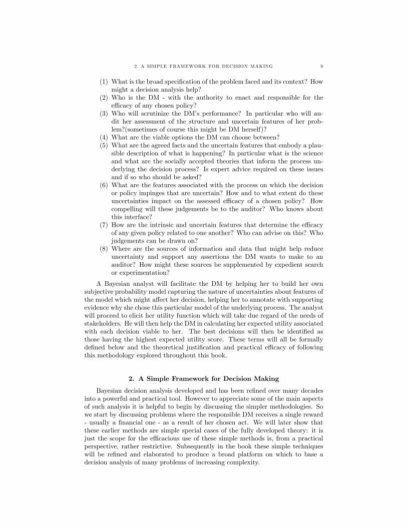
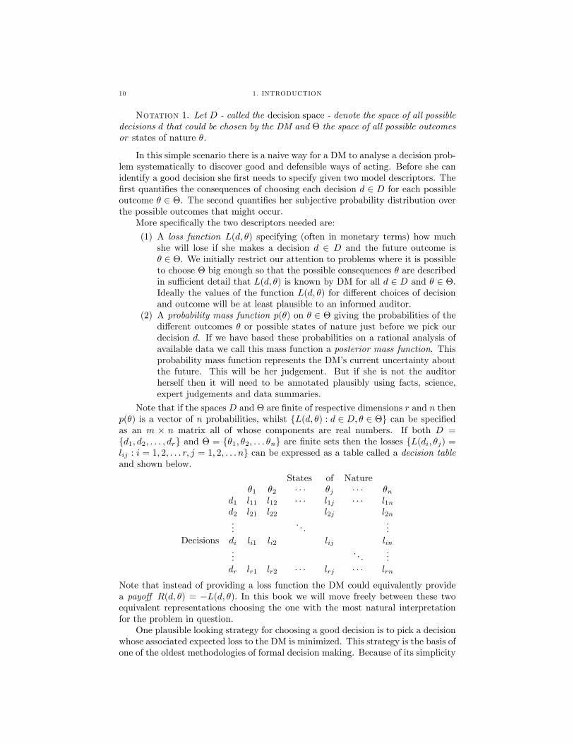
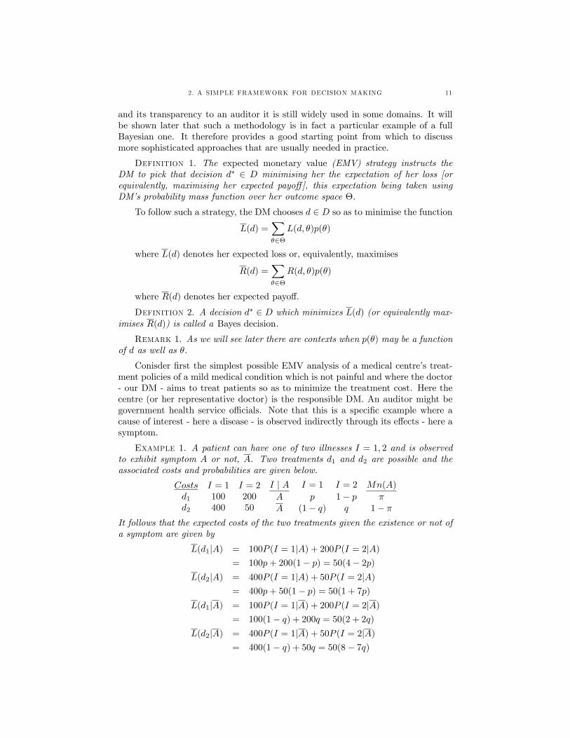


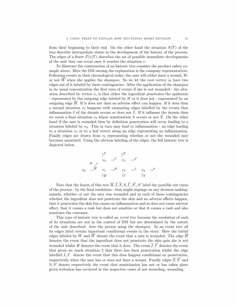

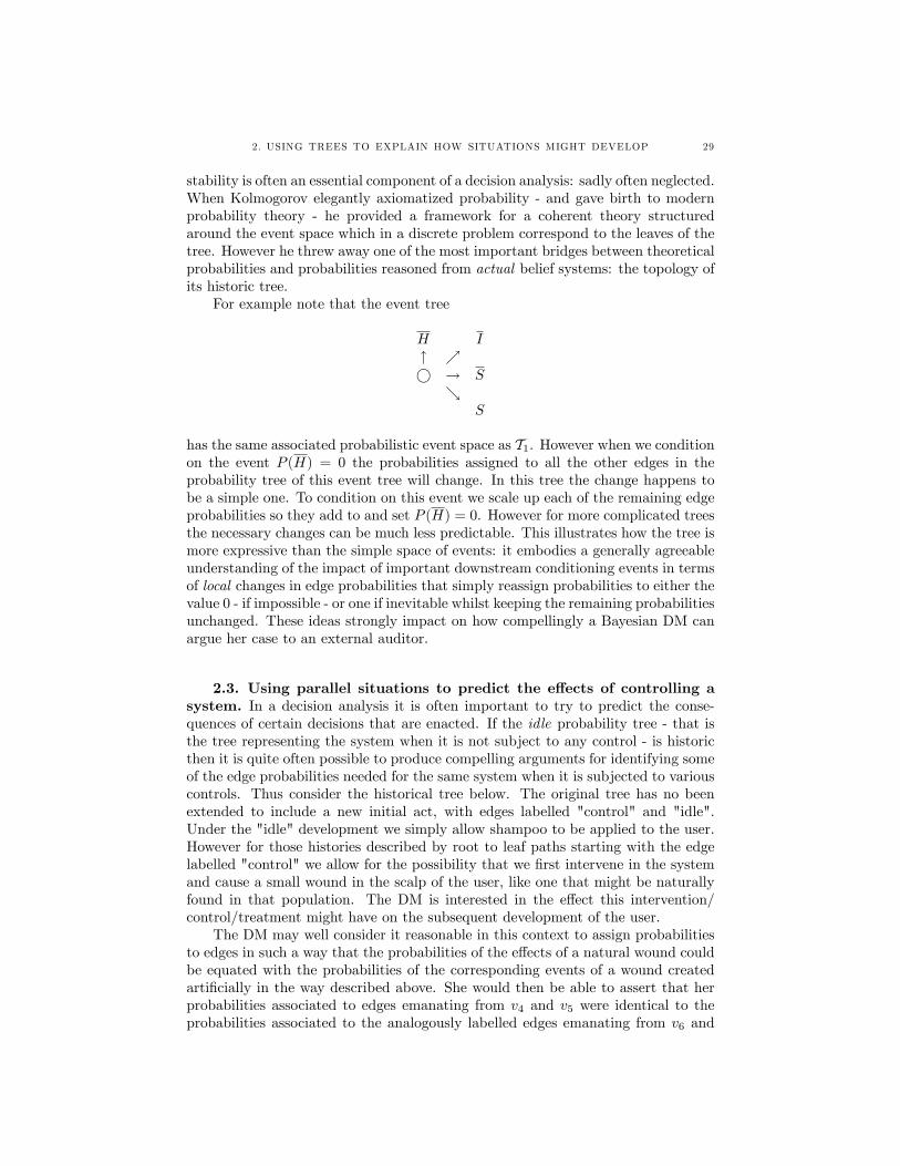


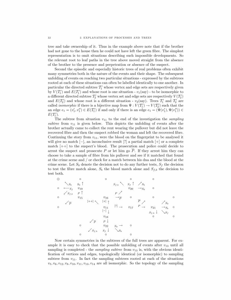


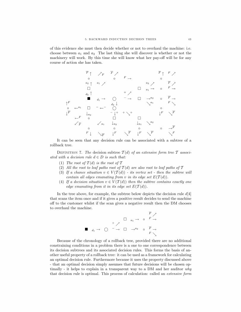
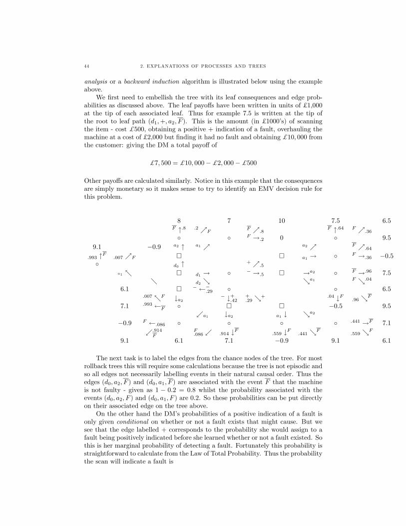
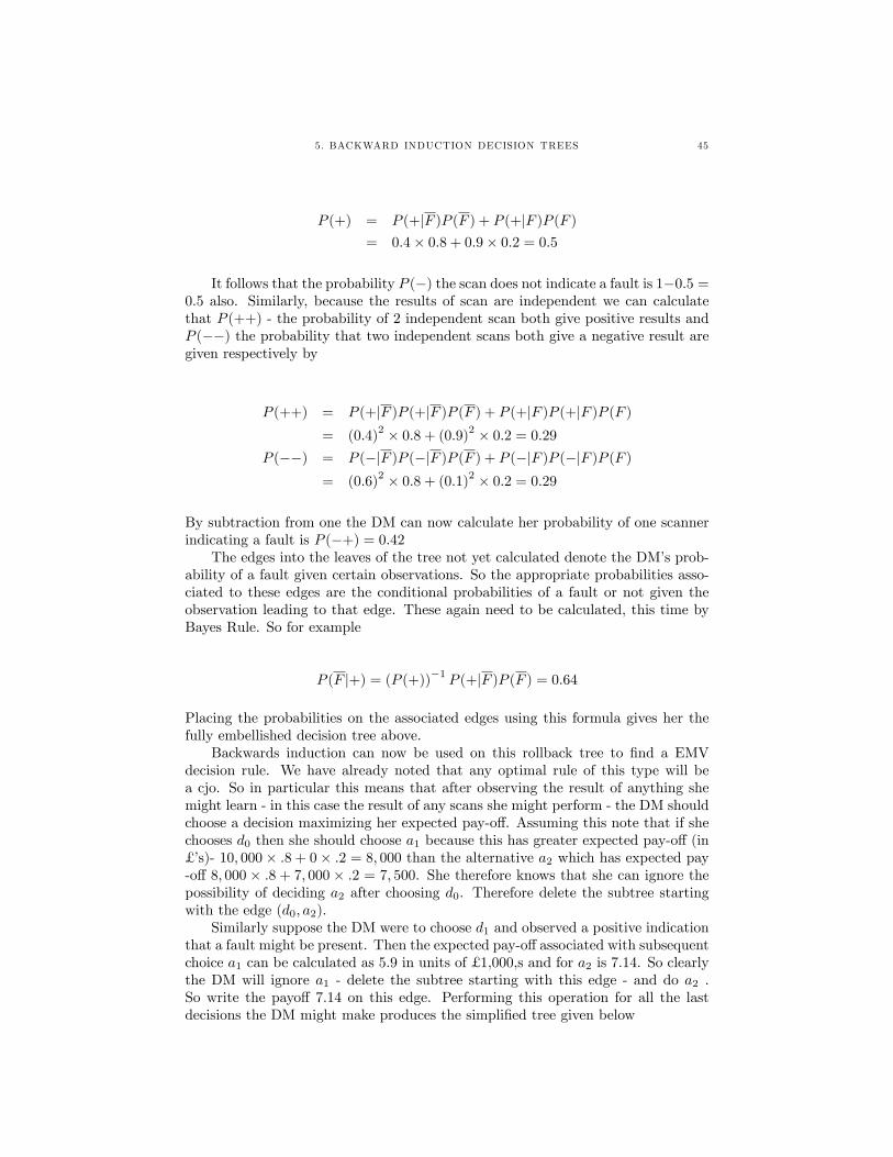
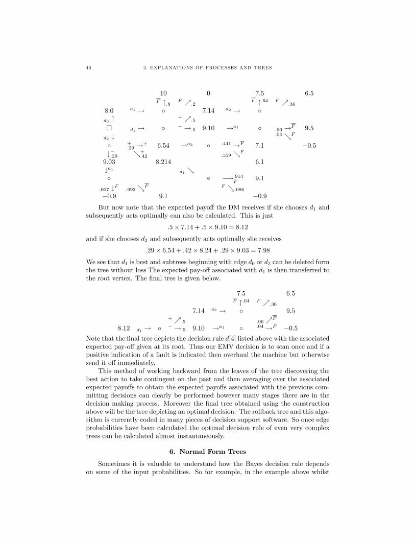


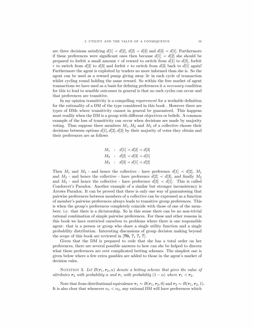


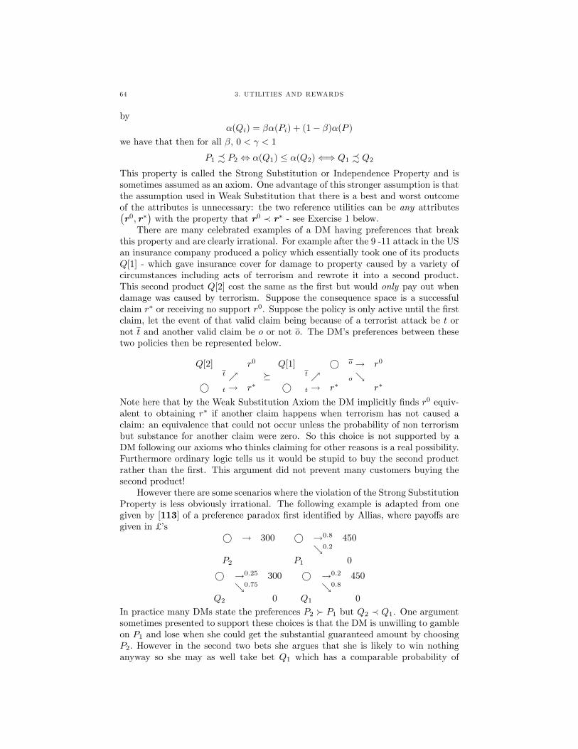
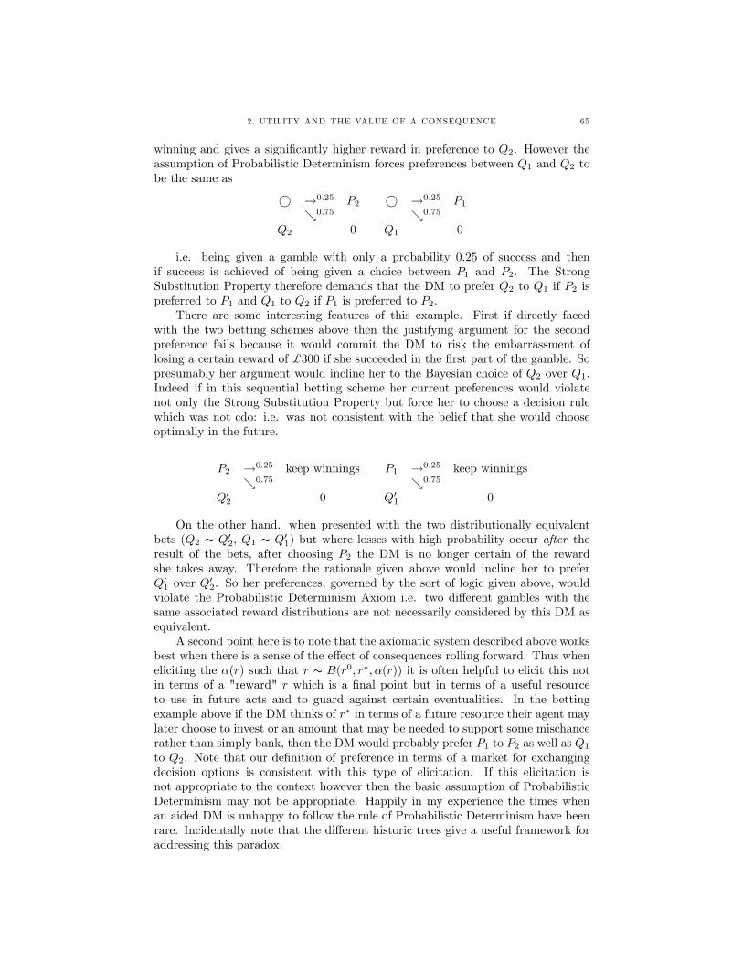
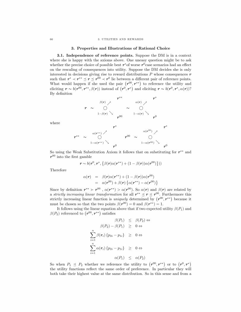
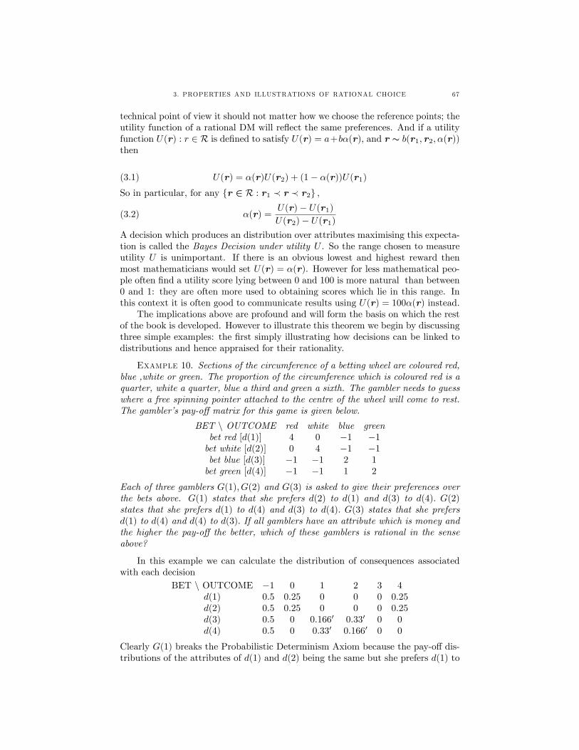
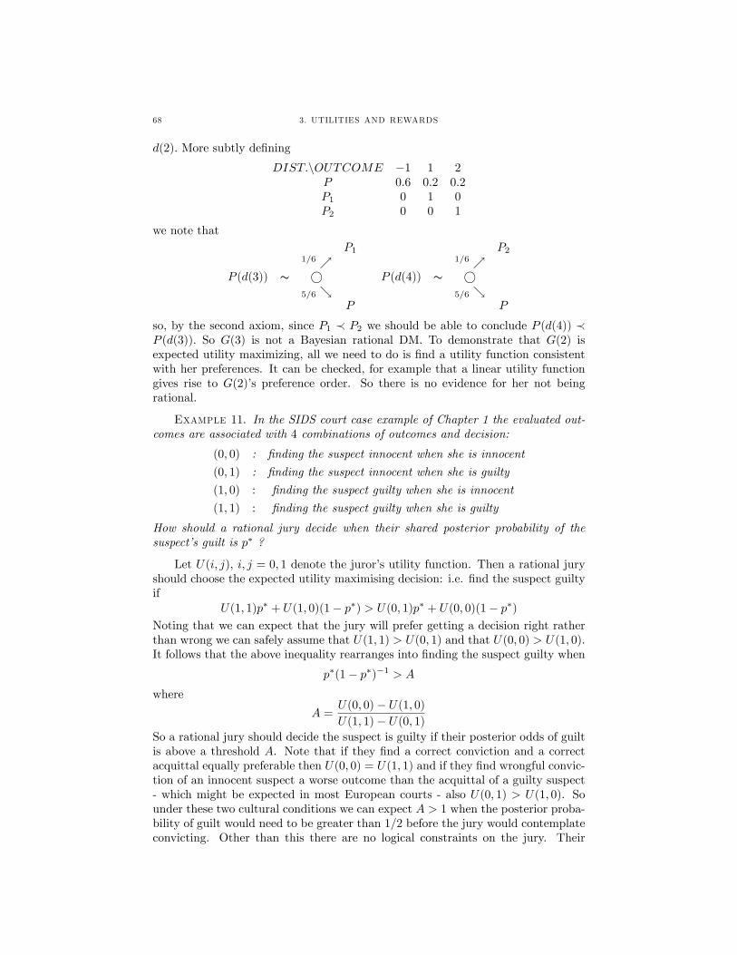


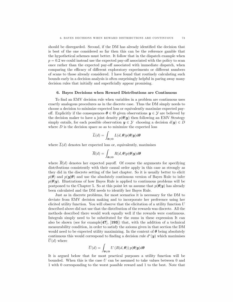


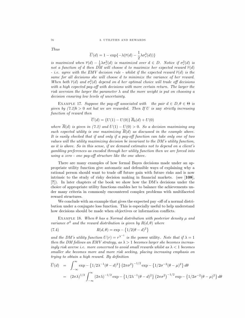
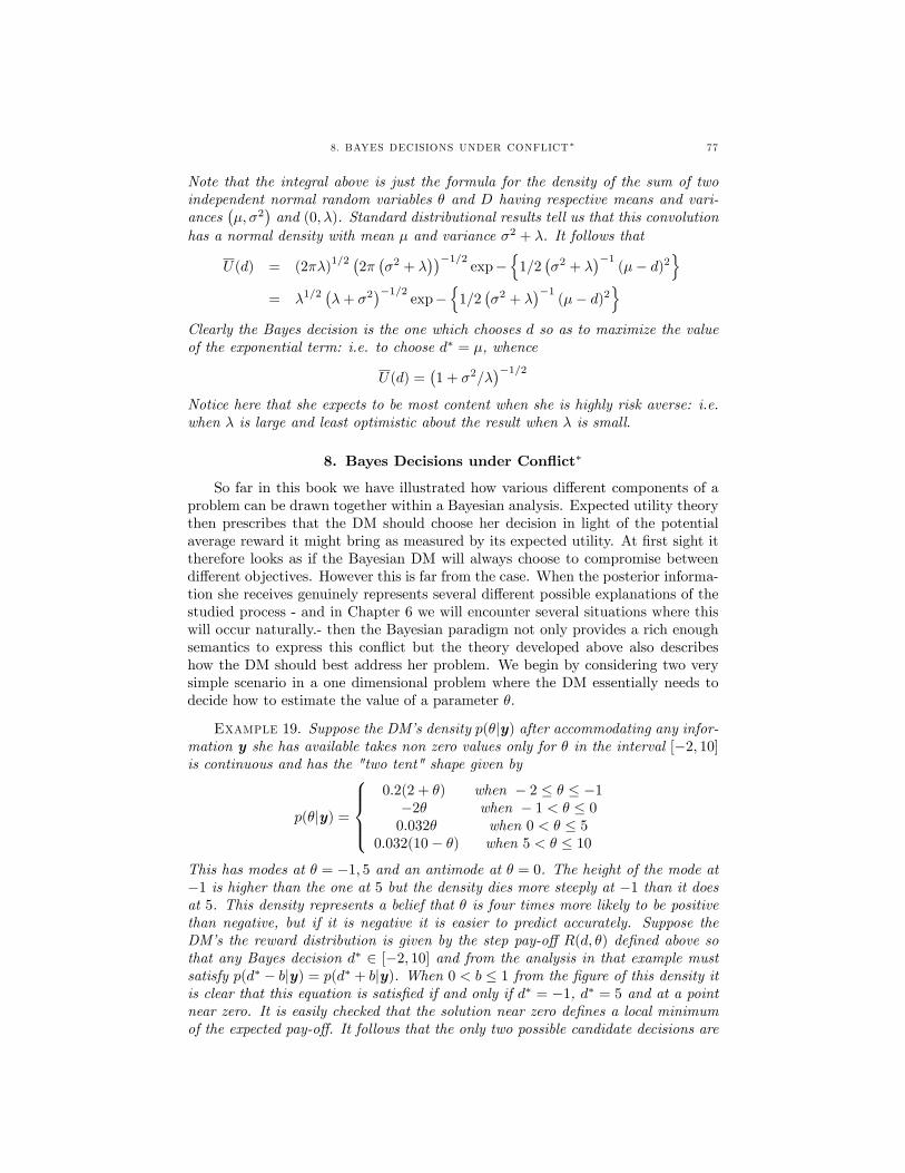
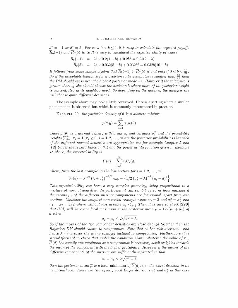

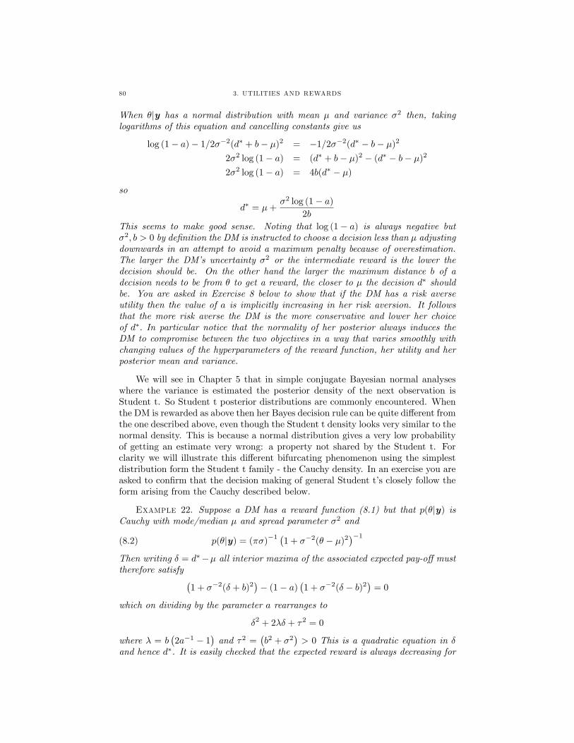


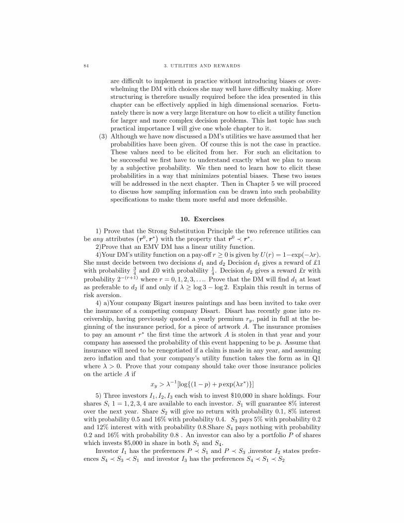


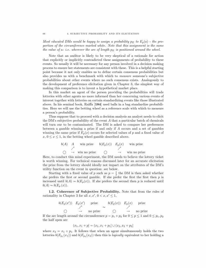

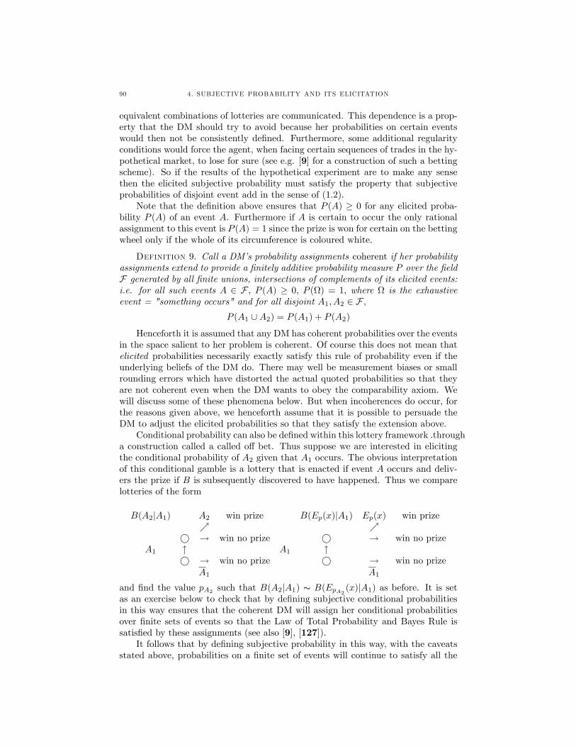
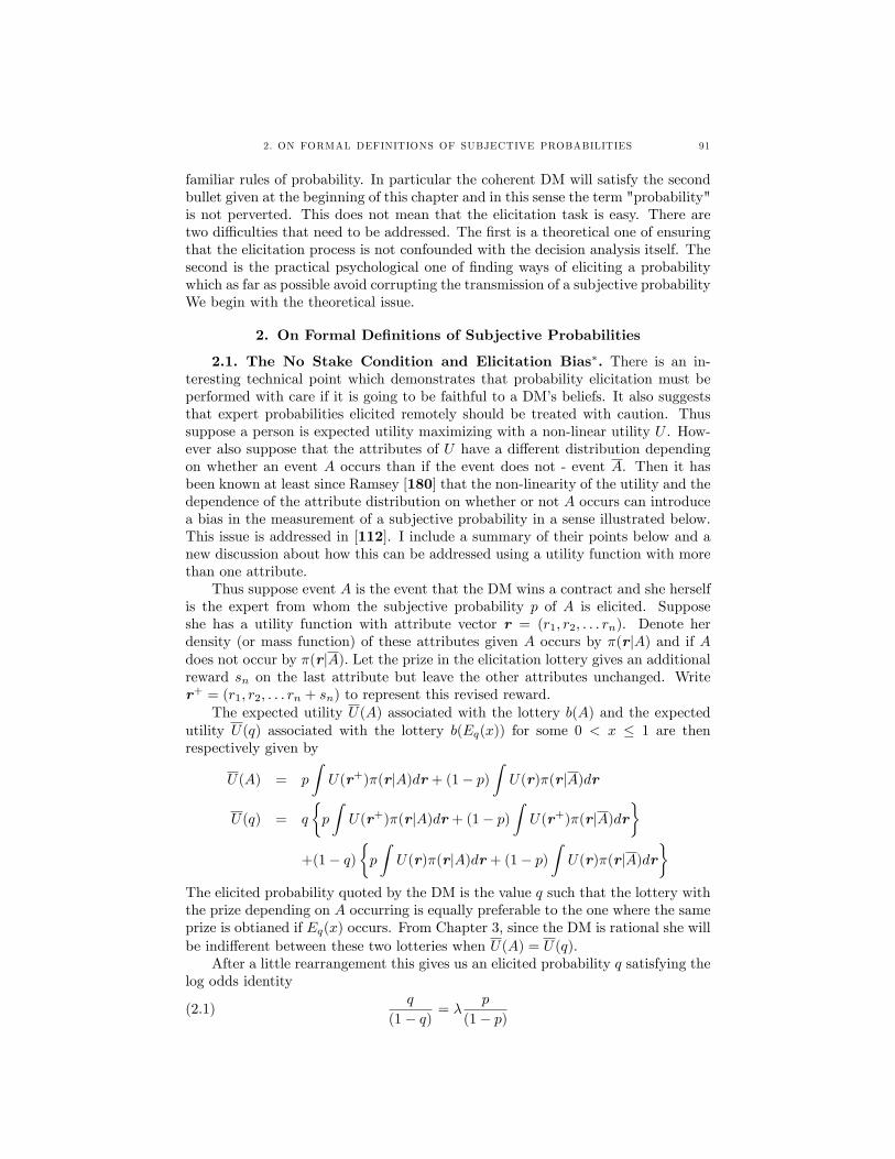
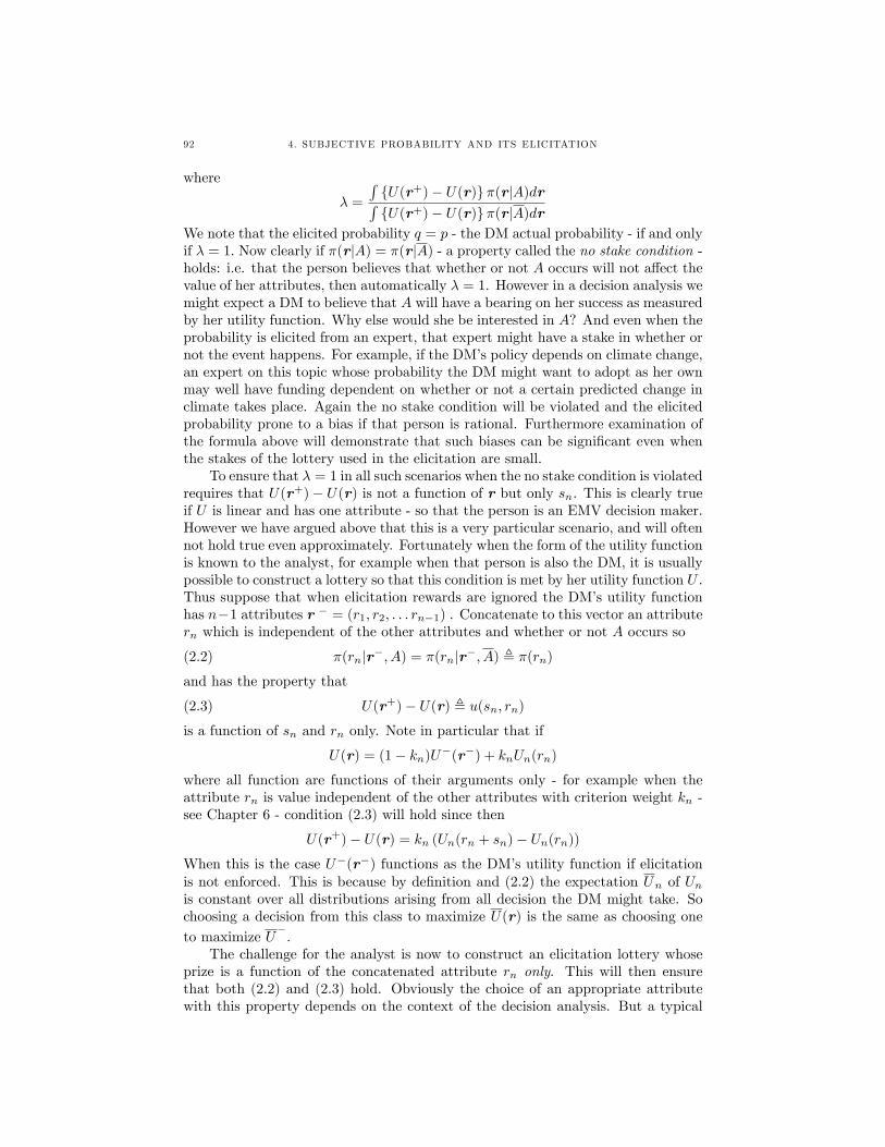


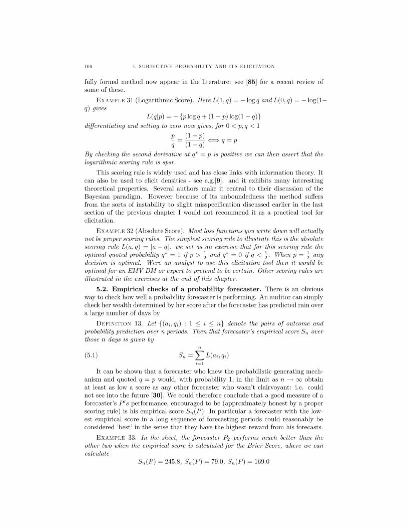
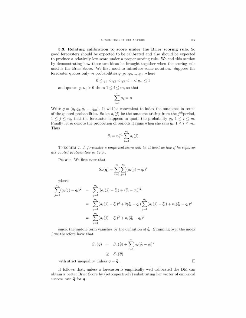


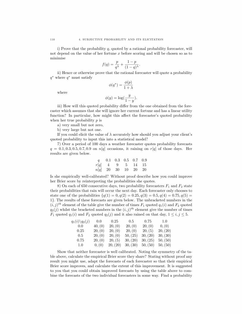


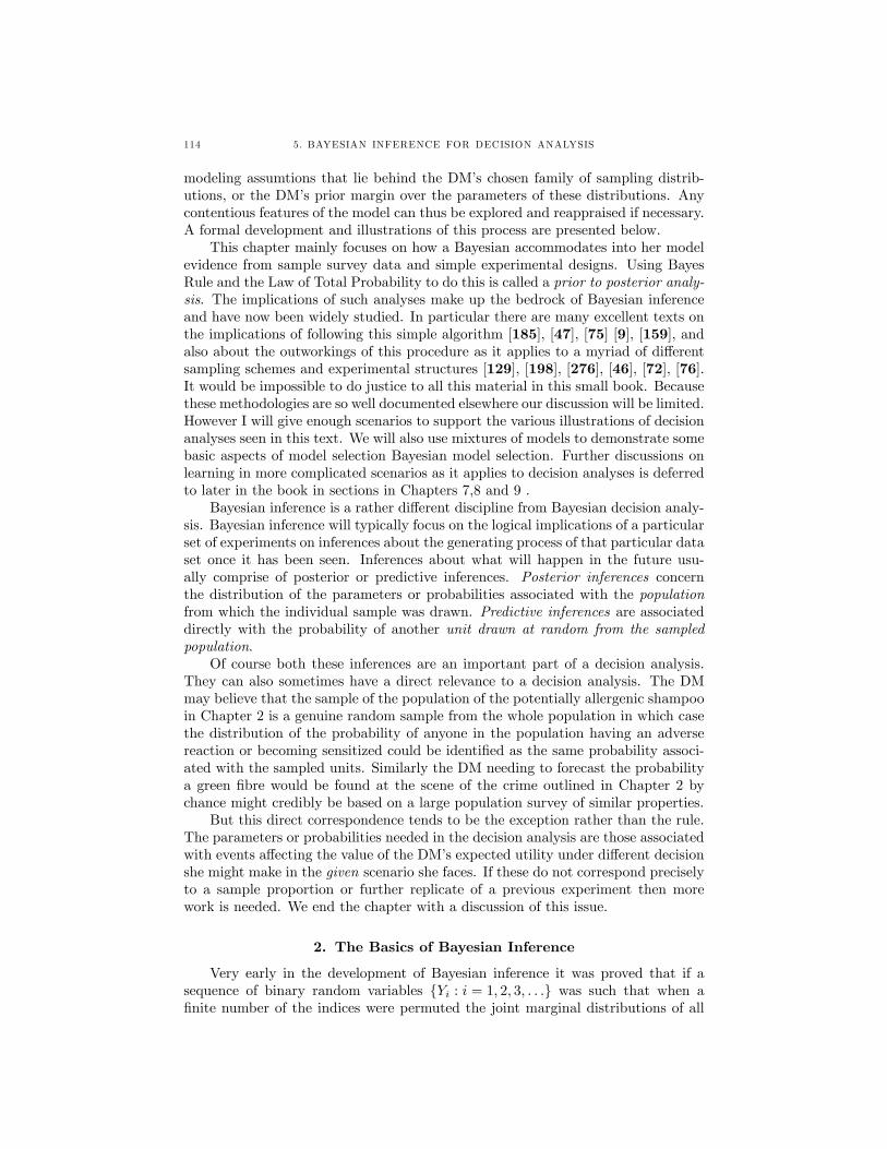


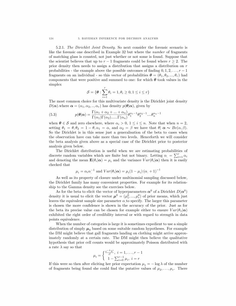
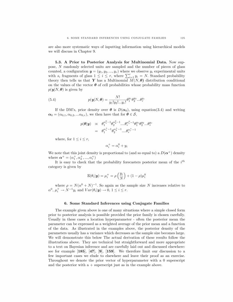
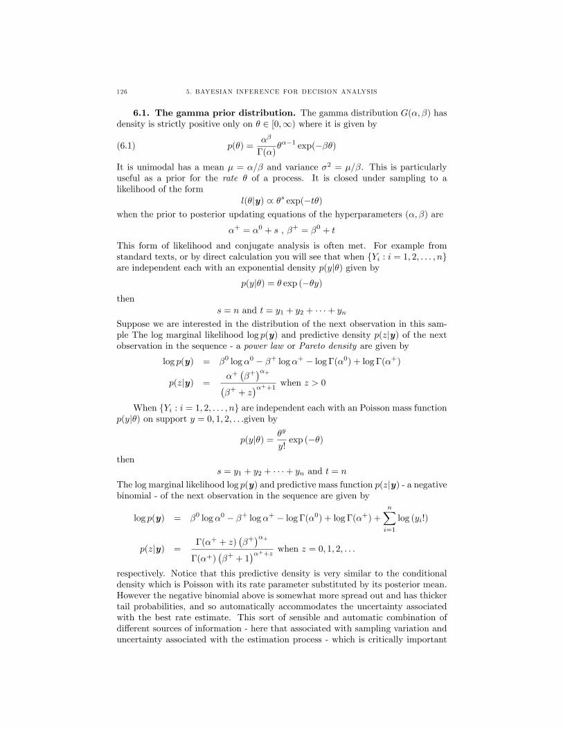


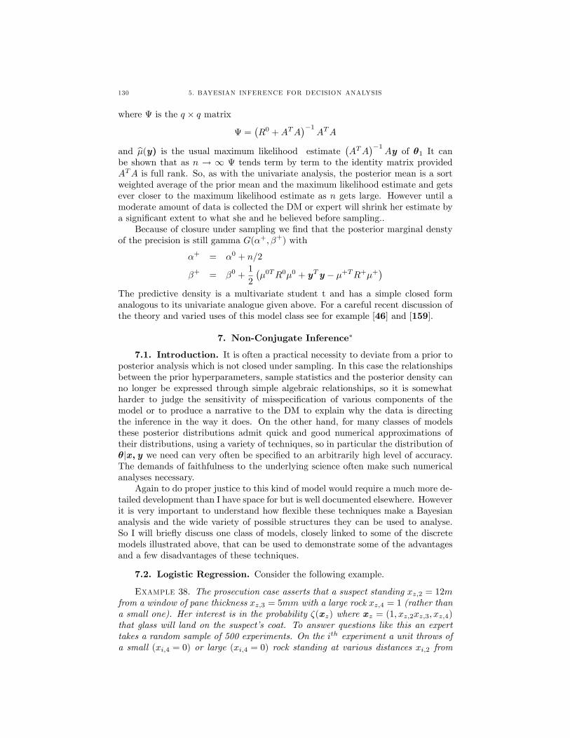


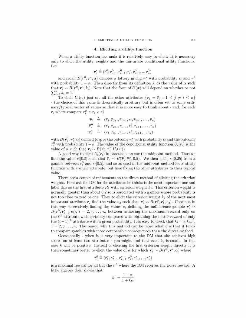
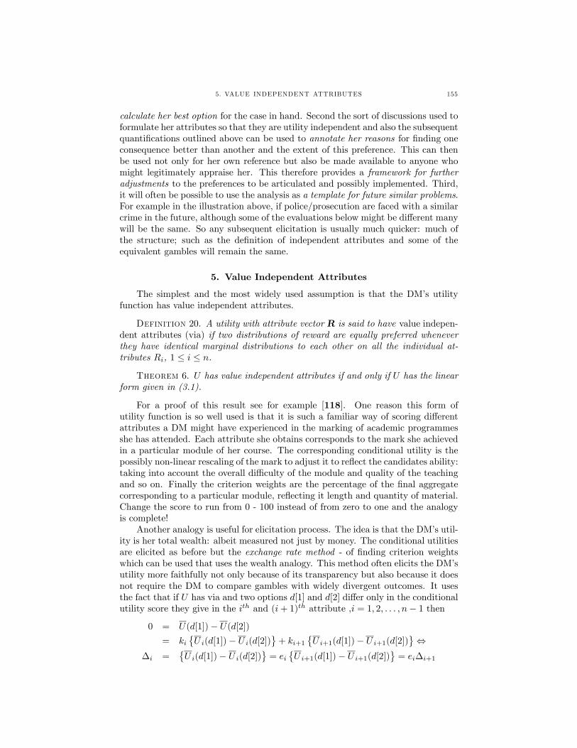
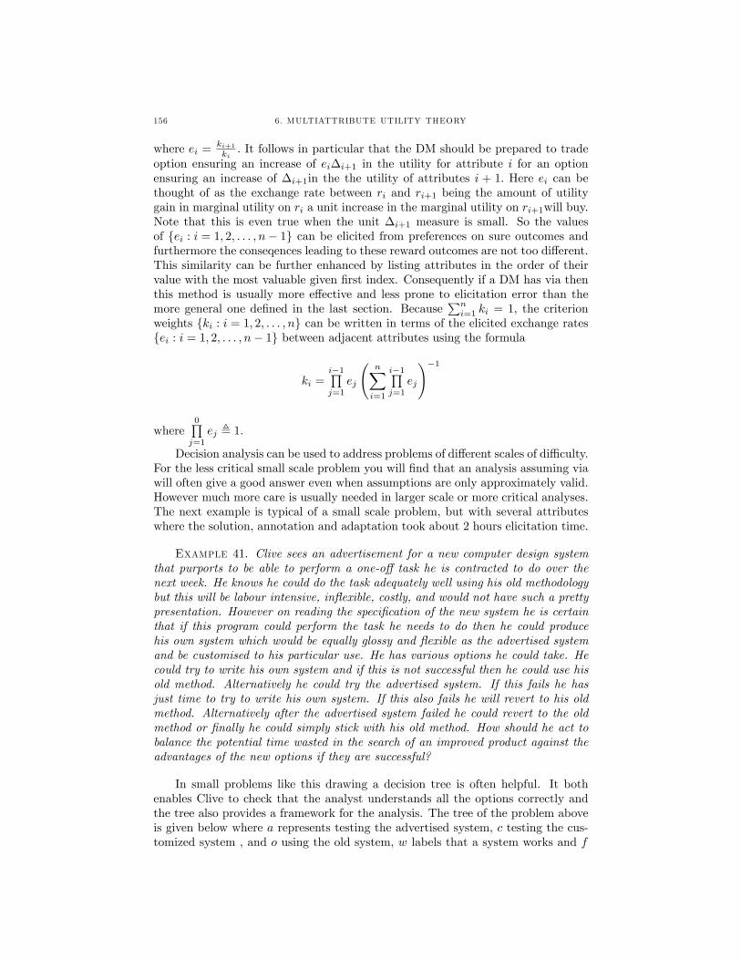
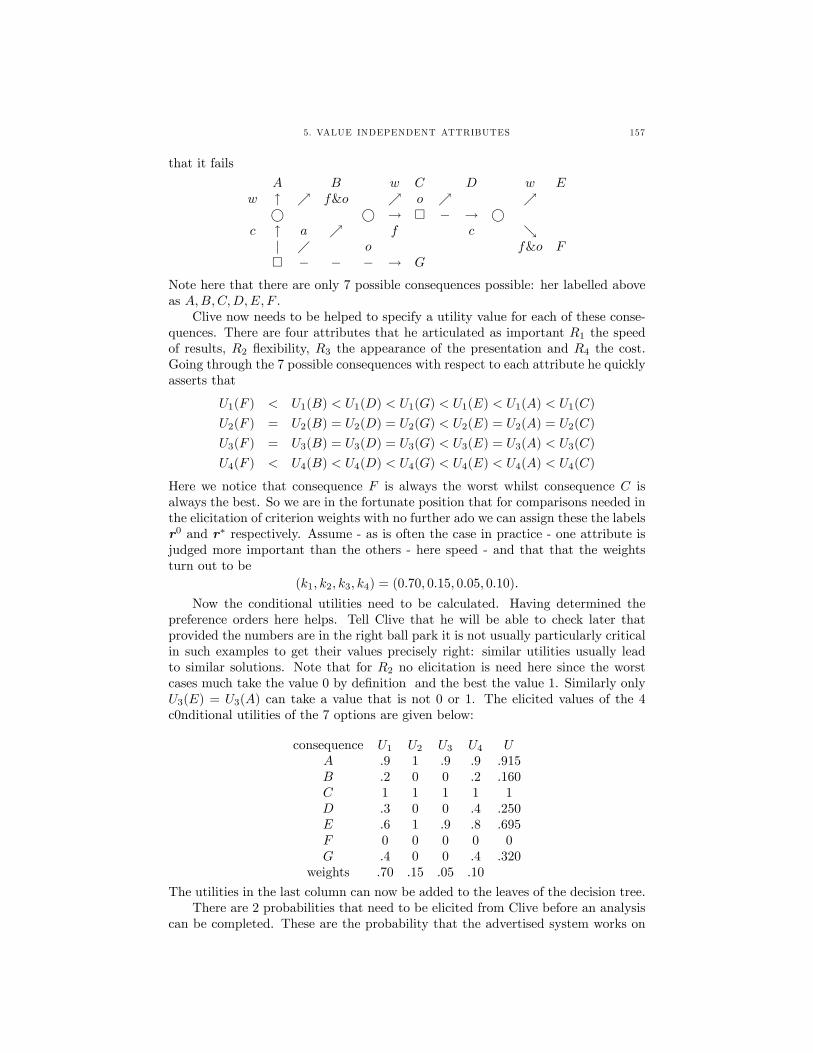
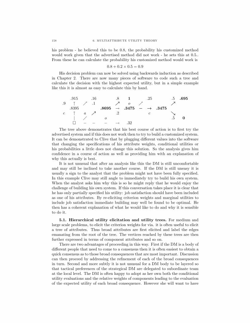


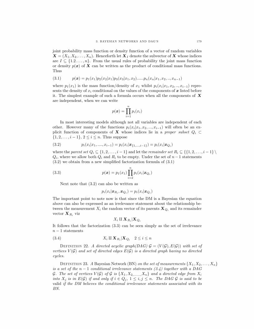
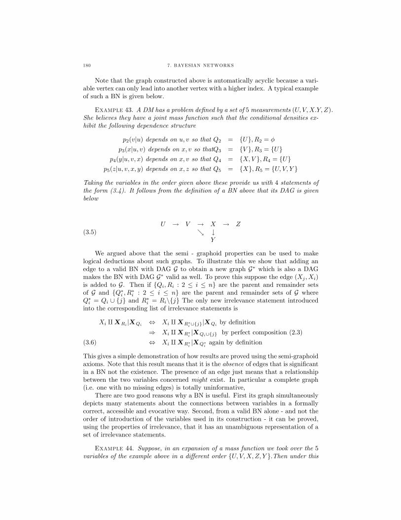


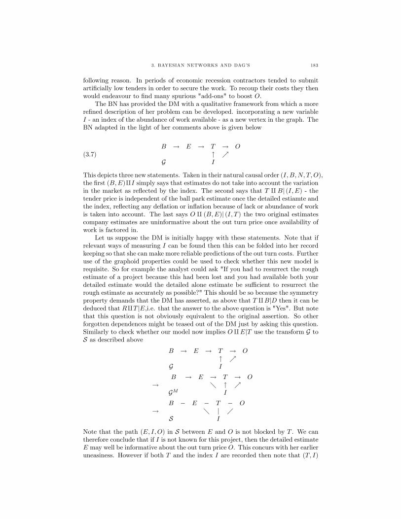
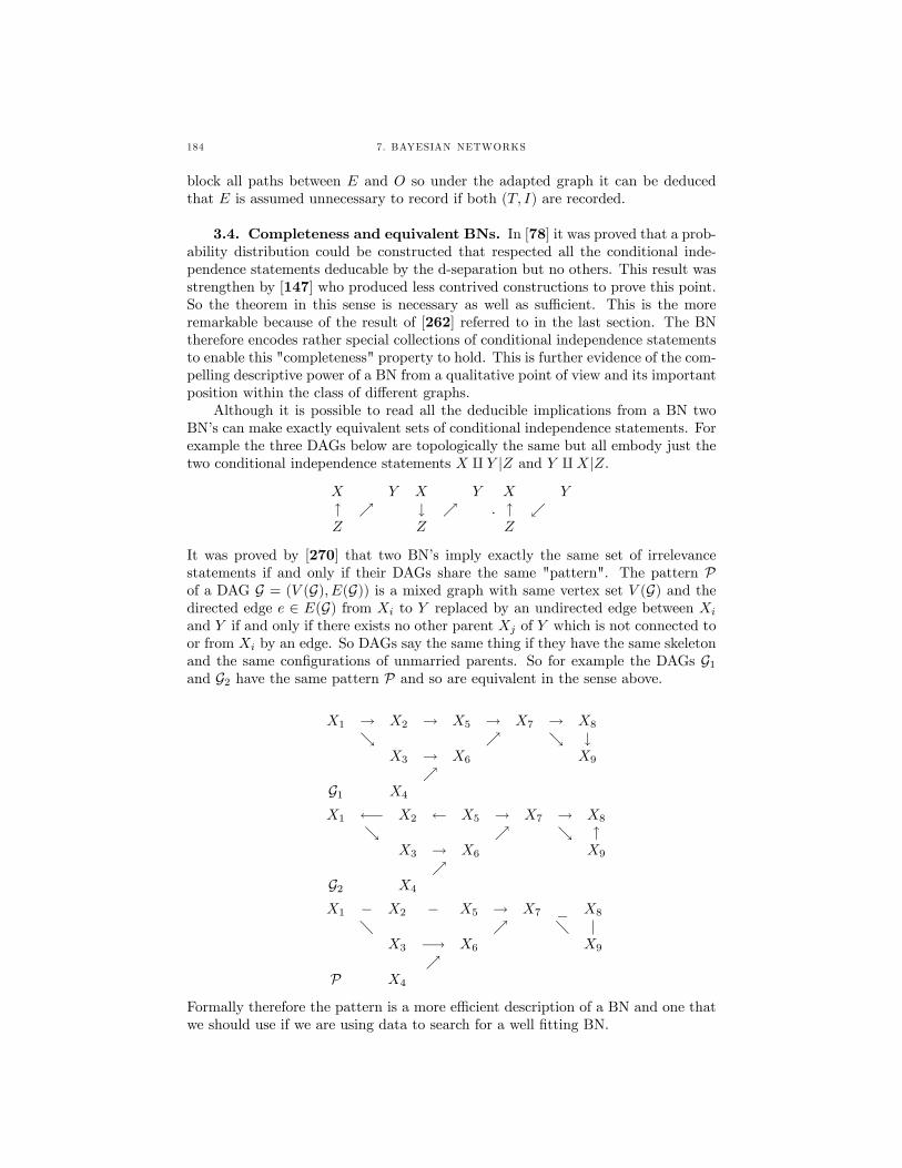


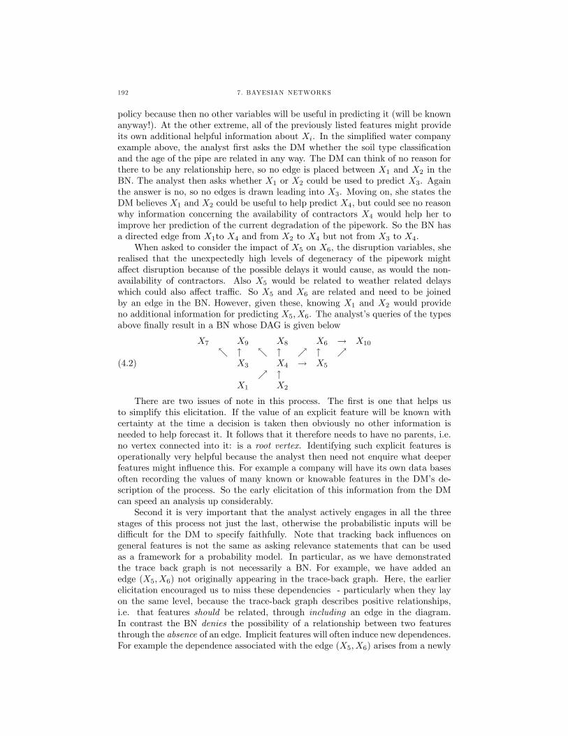


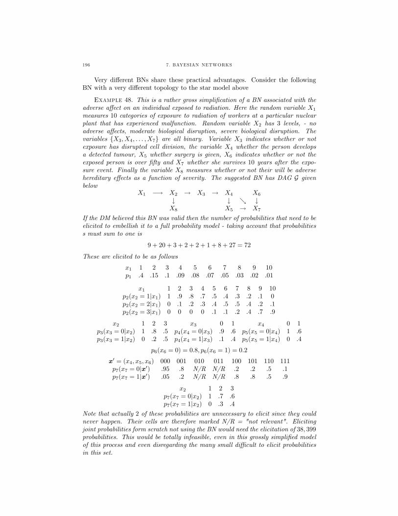


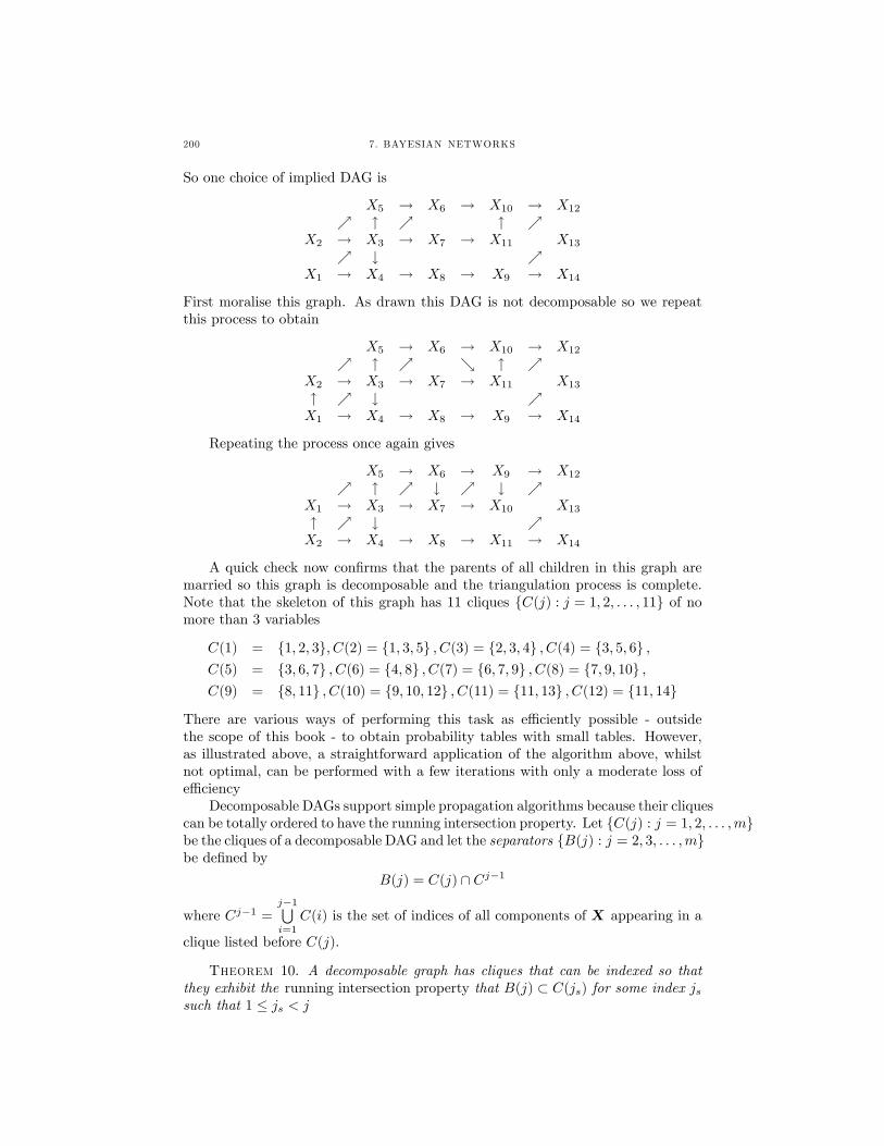

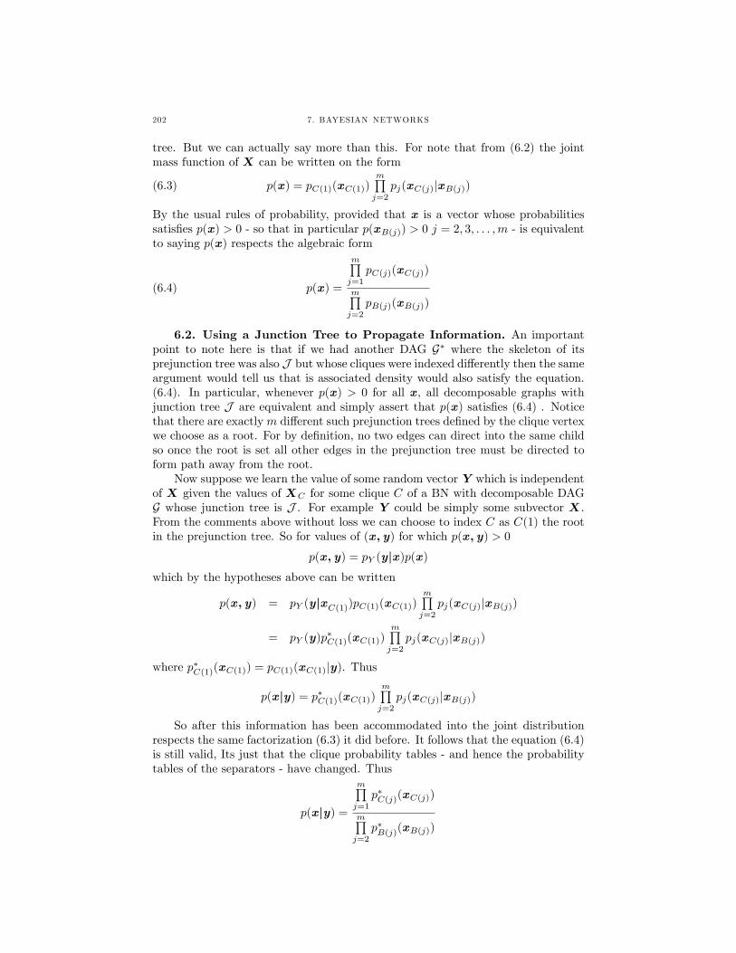


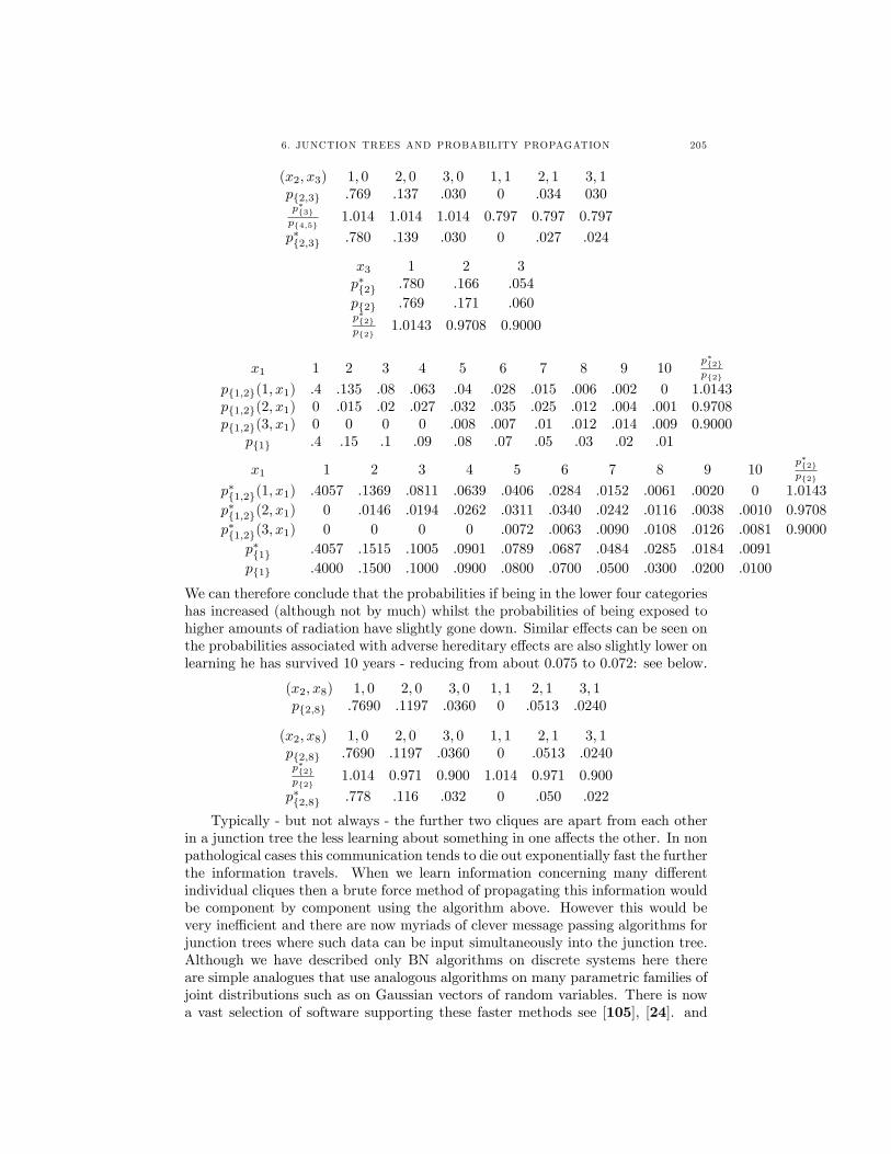

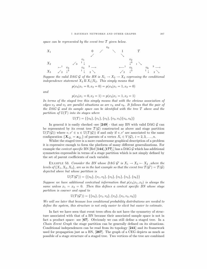
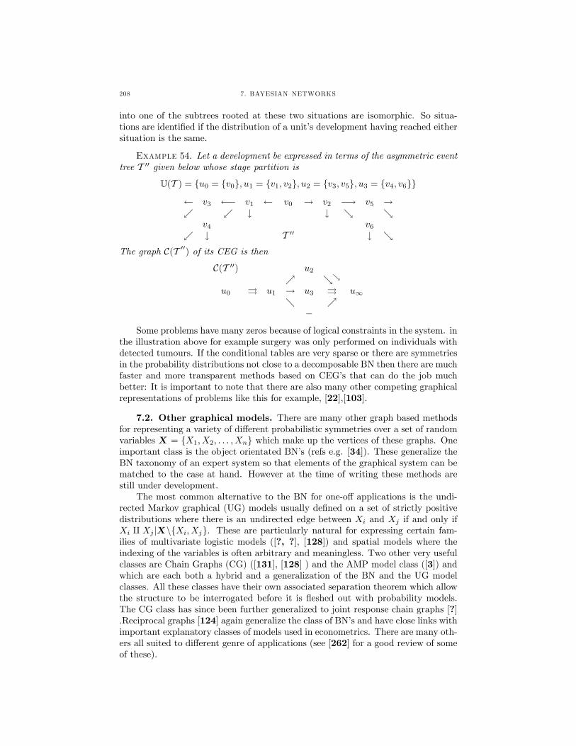


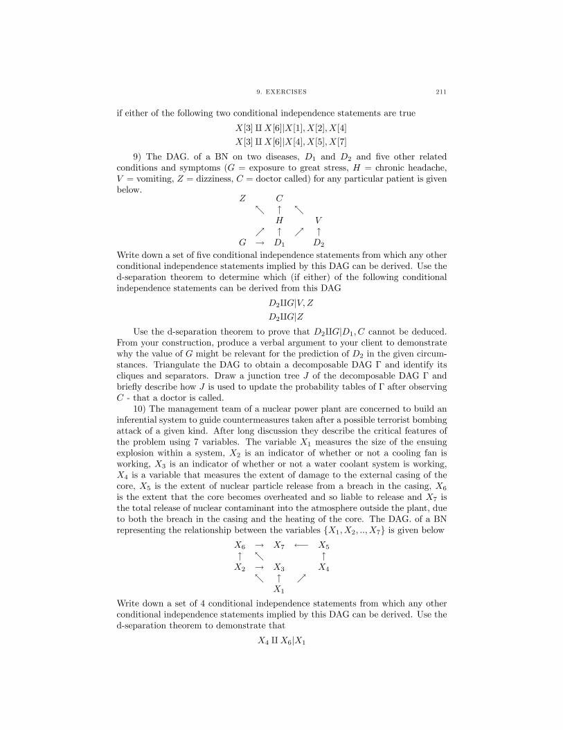


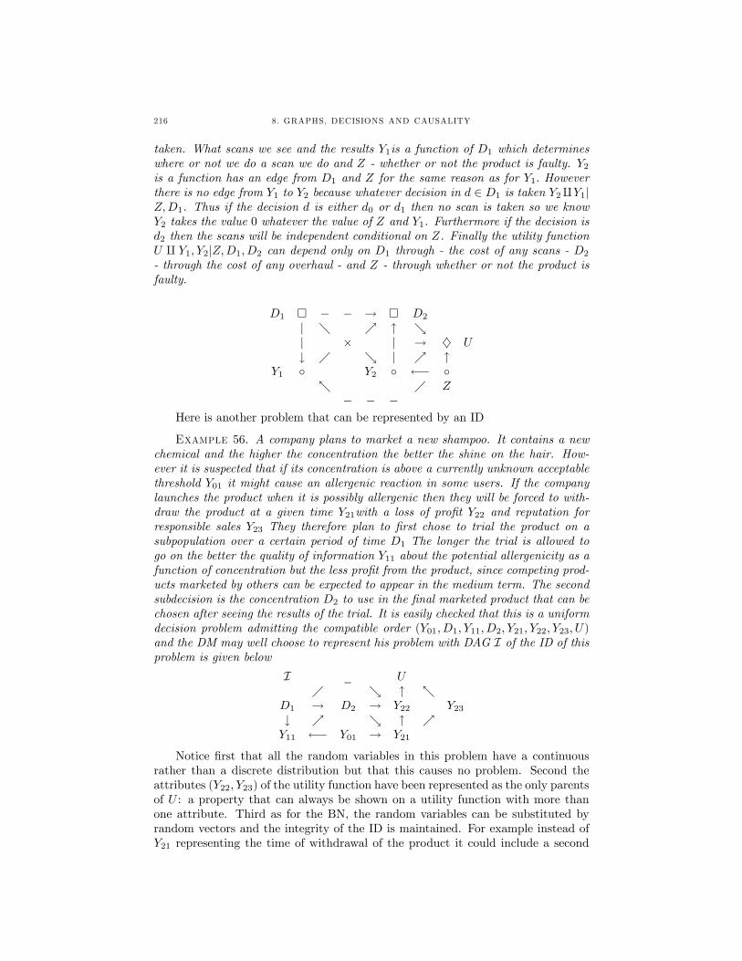
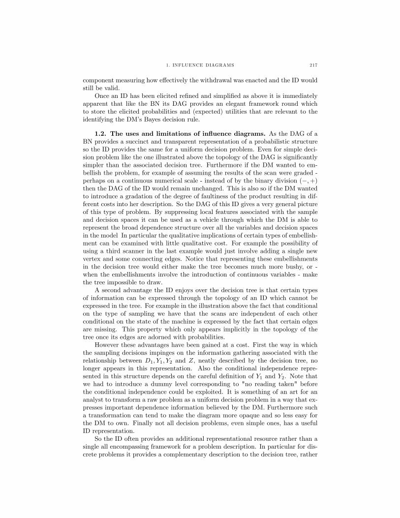

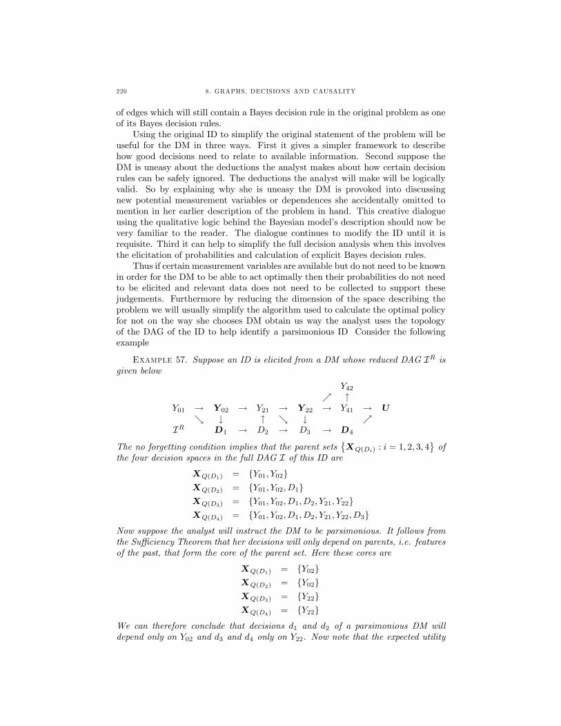
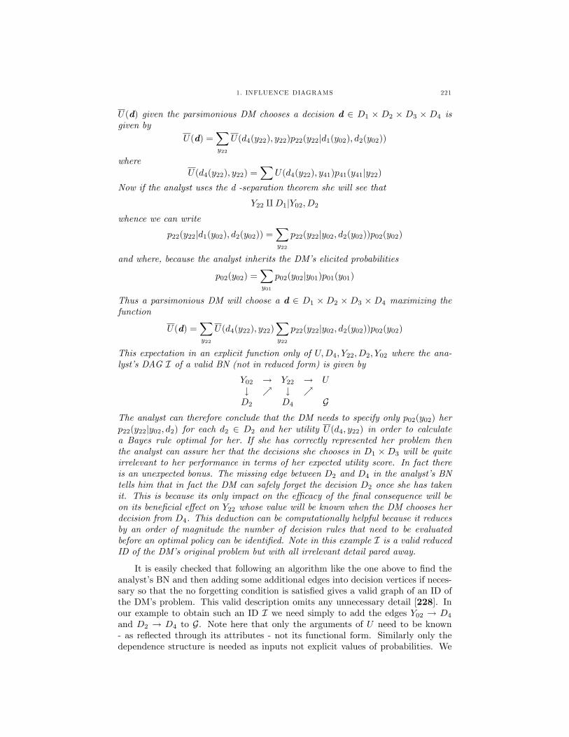


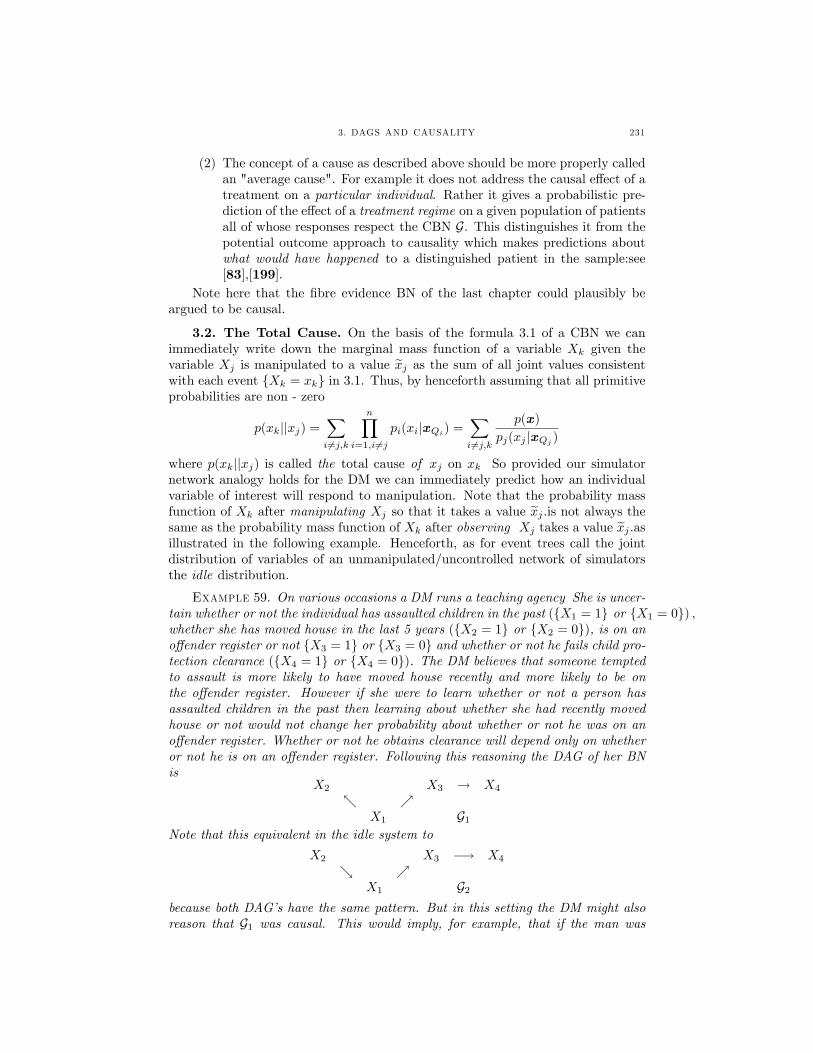

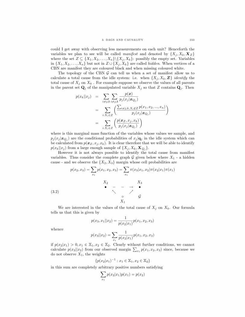

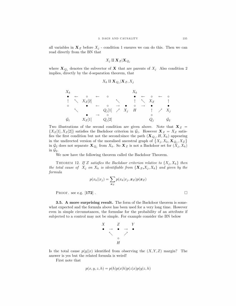


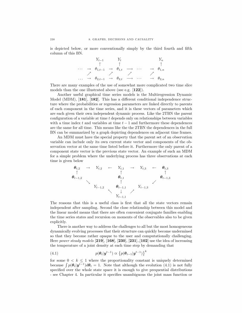


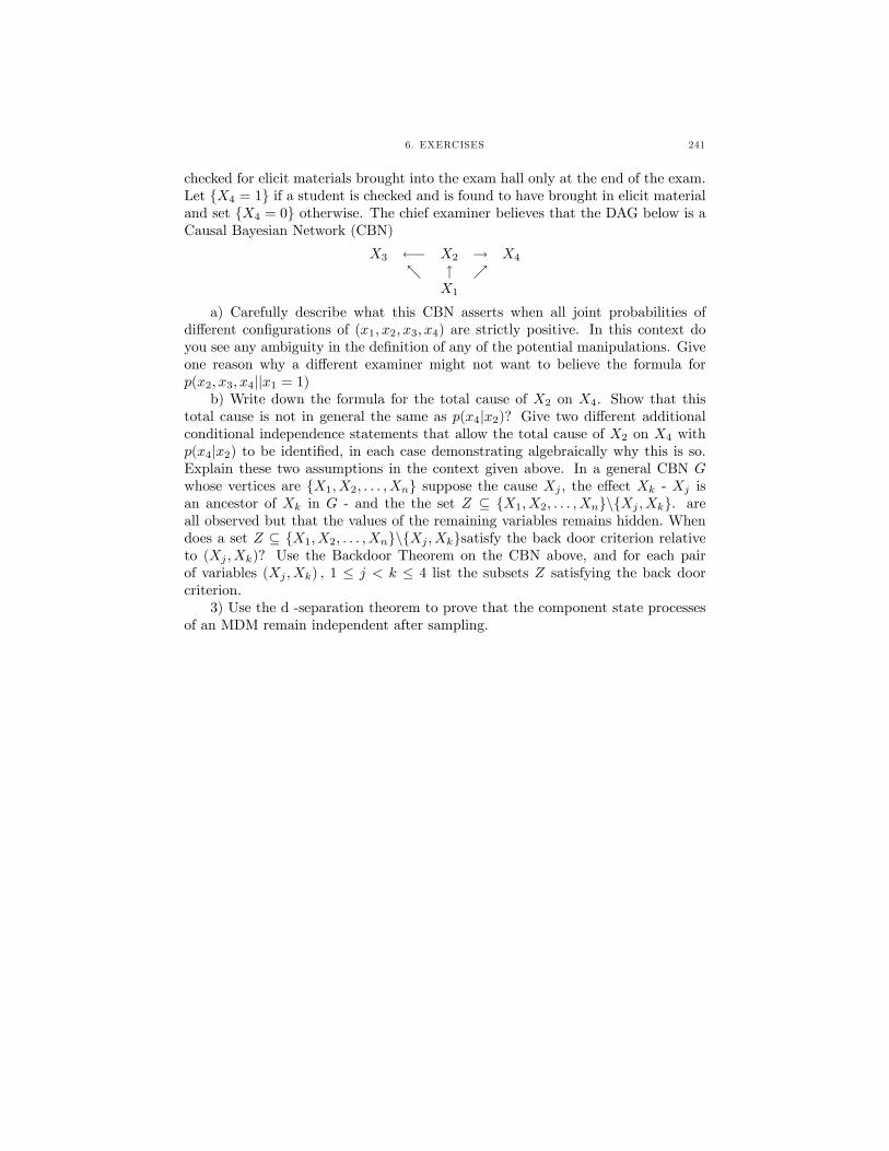


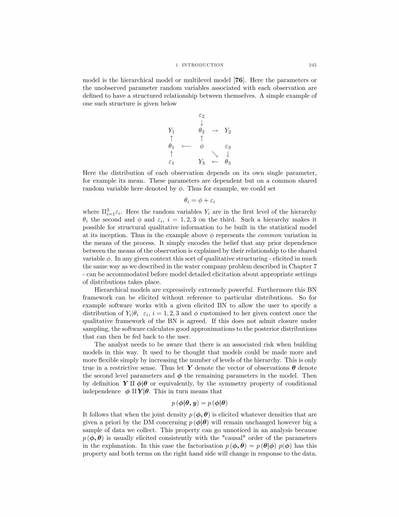
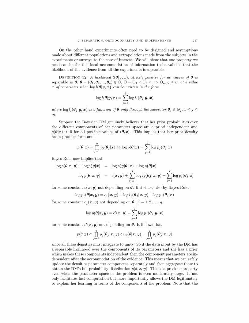
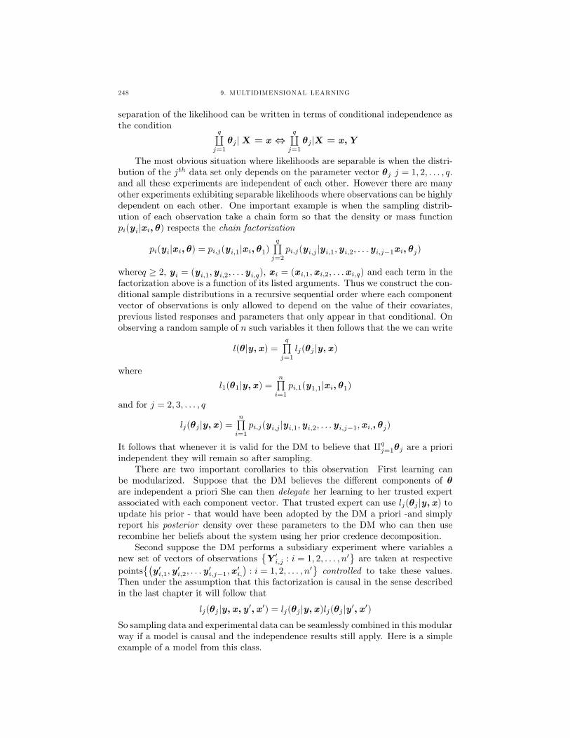


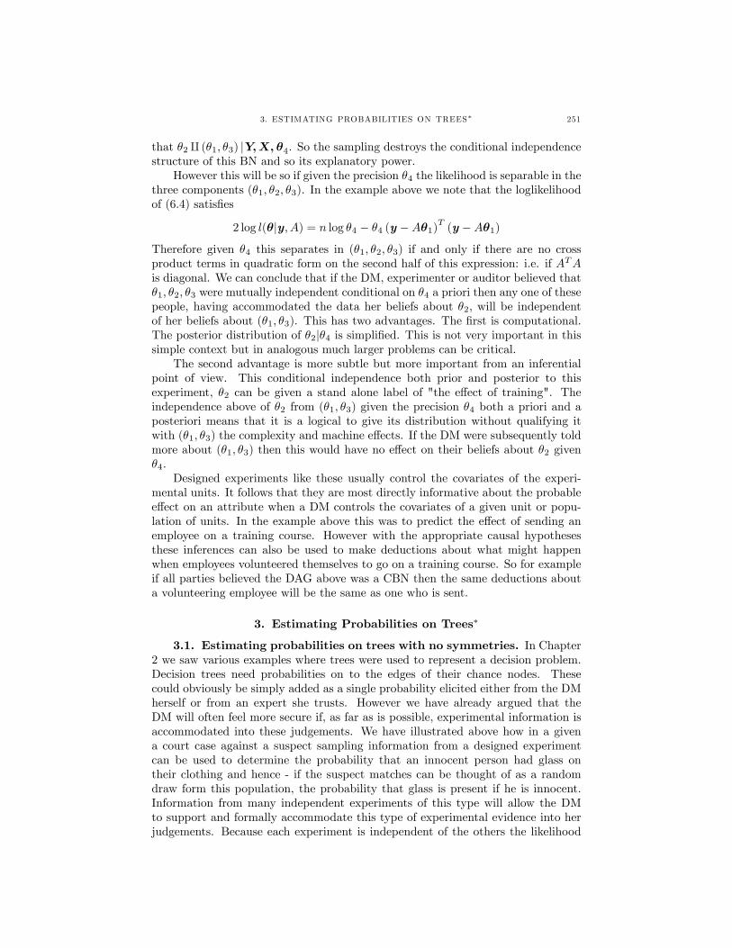

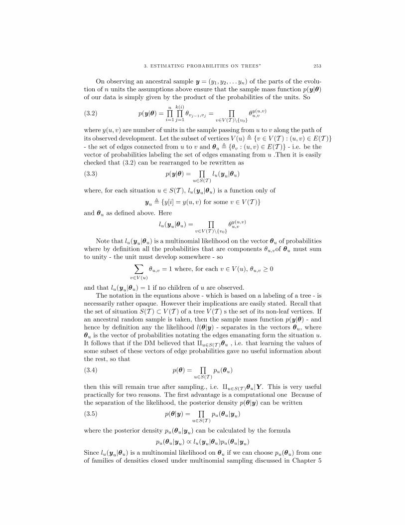
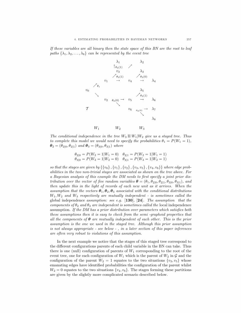


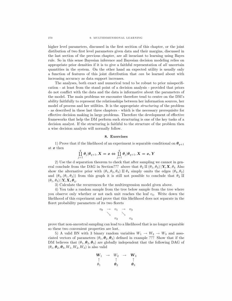


![[HTML5 BUG] 2,5D RTS Game in HTML5 by Dawid Lijewski](https://static.documents.pub/doc/80x56/55530872b4c9054e3f8b4ba1/html5-bug-25d-rts-game-in-html5-by-dawid-lijewski.jpg)


