Dipartimento di Scienze Economiche Università degli Studi di Brescia Via San Faustino 74/B – 25122 Brescia – Italy Tel: +39 0302988839/840/848, Fax: +39 0302988837 e-mail: [email protected]– www.eco.unibs.it These Discussion Papers often represent preliminary or incomplete work, circulated to encourage discussion and comments. Citation and use of such a paper should take account of its provisional character. A revised version may be available directly from the author(s). Any opinions expressed here are those of the author(s) and not those of the Dipartimento di Scienze Economiche, Università degli Studi di Brescia. Research disseminated by the Department may include views on policy, but the Department itself takes no institutional policy position. BAYESIAN ESTIMATION OF STOCHASTIC-TRANSITION MARKOV-SWITCHING MODELS FOR BUSINESS CYCLE ANALYSIS By Monica Billio Roberto Casarin Discussion Paper n. 1002
Transcript
Dipartimento di Scienze Economiche
Università degli Studi di Brescia Via San Faustino 74/B – 25122 Brescia – Italy
These Discussion Papers often represent preliminary or incomplete work, circulated to encourage discussion and comments. Citation and use of such a paper should take account of its provisional character. A revised version may be available directly from the author(s). Any opinions expressed here are those of the author(s) and not those of the Dipartimento di Scienze Economiche, Università degli Studi di Brescia. Research disseminated by the Department may include views on policy, but the Department itself takes no institutional policy position.
BAYESIAN ESTIMATION OF STOCHASTIC-TRANSITION
MARKOV-SWITCHING MODELS FOR BUSINESS CYCLE ANALYSIS
By
Monica Billio Roberto Casarin
Discussion Paper n. 1002
Bayesian Estimation of Stochastic-transitionMarkov-switching Models for Business Cycle
Analysis
Monica Billio §¶‖ and Roberto Casarin†‖
†Dept. of Economics, University of Brescia§Dept. of Economics, University of Venice¶School for Advanced Studies in Venice
‖GRETA, Venice
AbstractWe propose a new class of Markov-switching (MS) models for businesscycle analysis. As usually done in the literature, we assume that theMS latent factor is driving the dynamics of the business cycle butthe transition probabilities can vary randomly over time. Transitionprobabilities are generated by random processes which may account forthe stochastic duration of the regimes and for possible stochastic relationsbetween the MS probabilities and some explanatory variables, such asautoregressive components and exogenous variables. The presence oflatent factors and nonlinearities calls for the use of simulation-basedinference methods. We propose a full Bayesian inference approach whichcan be naturally combined with Monte Carlo methods. We discuss thechoice of the priors and a Markov-chain Monte Carlo (MCMC) algorithmfor estimating the parameters and the latent variables. We provide anapplication of the model and of the MCMC procedure to data of Euroarea. We also carry out a real-time comparison between different modelsby employing sequential Monte Carlo methods and some concordancestatistics, which are widely used in business cycle analysis.
Keywords: Markov-switching Models; Stochastic Duration Models;Bayesian Inference; Markov-Chain Monte Carlo; Sequential Monte Carlo.
AMS classification: 62G07, 62M20, 62P20, 91B84.¶E-mail: [email protected]. Presented at ERCIM Workshop on Computing and Statistics,
2008; and the 3rd ICEEE, 2009.
1
1 Introduction
Turning points detection and forecasting of the economic activity level arechallenging problems in business cycle analysis. In this paper we consider amodel-based framework and a Bayesian inference approach to deal with theseissues.
Early contributions in the non-linear literature applied Markov Switching(MS) models (see for example Goldfeld and Quandt (1973) and Hamilton (1989))and threshold autoregressive models (see Tong (1983) and Potter (1995)) tocapture turning points and model the asymmetry in the business cycle dynamics.
These contributions have been extended in many directions. Kim (1994)applies MS to dynamic linear models. In this case the Hamilton’s filter is uselessand he proposes a Bayesian approach for inference. Kim and Nelson (1999b)provide a complete introduction to inference methods based on Markov-chainMonte Carlo (MCMC) for MS state space models.
In the basic MS models for business cycle the switching process indicatesthe phase of the economic cycle and may assume at least two regimes, whichare usually interpreted as: positive growth trend and negative growth trend.Kim and Murray (2001) and Kim and Piger (2000) consider MS models withthree-regimes (recession, high-growth and normal-growth).
Other extensions are in Sichel (1991), Watson (1994), Diebold and Rudebusch(1996), Durland and McCurdy (1994) and Filardo (1994), which assume that theMS transition probabilities depend on the duration of the current phase of thecycle and thus are time-varying. Moreover, Billio and Casarin (2009) considerstochastic transition probabilities. Finally some multivariate extensions to theHamilton (1989) model can be found in Diebold and Rudebusch (1996) andKrolzig (1997, 2004).
In the present work we combine a state space approach to the businesscycle with the possibility to consider a non homogeneous MS model. Thefirst contribution is to assume that the transition probabilities of the Markov-switching process vary randomly over time. More specifically we assume thatthe probabilities are stochastic processes with beta distributed innovations. Themain advantages of using a beta random variables is that it is naturally definedon a bounded interval and is a flexible probabilistic model. See Ferrari andCribari-Neto (2004) for an introduction to beta regression models.
Models with stochastic transition have been already proposed in econometricsby Gagliardini and Gourieroux (2005) in a continuous time setting. In that workthe probability of transition of the credit quality from one rating class to anotherone is modelled as a Jacobi diffusion process, which is naturally defined on abounded interval. The ergodic distribution of the Jacobi process is a beta. Thisprobabilistic fact suggests us that a beta noise process could be a very good
2
candidate process for modelling, in a discrete-time setting, random fluctuationson bounded intervals.
The use of random transition probabilities implies that the duration of thedifferent regimes is stochastic and has thus a dynamics. The dynamics of theMS transition probabilities in the existing works is usually modelled by means ofa deterministic (e.g. linear-logistic) relationship between the probabilities and aset of explanatory variables. We introduce a residual term in order to accountfor unexplained variations in duration. Moreover, the variations in the MSprobabilities and in the duration can be explained thanks to an autoregressivestructure.
In this work we introduce a very flexible parameterization which allows for aeasy identification of the location and scale parameters involved in the model. Inthis sense the proposed model represents an extension of the stochastic transitionmodel proposed in Billio and Casarin (2009). The proposed parameterizationallow us to model directly the mean of the process (i.e. the transitionprobabilities) and make easier the inference procedure on the parameter.
Another relevant contribution of the present work is to propose a full Bayesianinference approach for random transition MS models. We refer the reader toBauwens, Lubrano and Richard (1999) for an introduction to Bayesian inferencefor dynamic models. Kim and Nelson (1999b) provide a review on Bayesianinference method for MS models. Moreover, we follow an inference approachbased on Monte Carlo simulation methods, see Billio, Casarin and Sartore (2007)for an updated review on the simulation-based inference methods for businesscycle models and Billio, Monfort and Robert (1999) for MCMC-based inferencefor MS ARMA processes. We follow a data-augmentation approach and proposea MCMC algorithm for jointly estimating the latent MS autoregressive processand the stochastic transition probabilities. Finally, we provide an application tothe business cycle of the Euro area and employ Sequential Monte Carlo (SMC)methods, also known as Particle Filters (Doucet, Freitas and Gordon (2001)), toobtain a sequential comparison between some competing models.
The work is structured as follows. Section 2 introduces a probabilistic statespace representation of dynamic models and presents a new MS model withstochastic transition probabilities. Section 3 proposes a Bayesian inferenceapproach for the stochastic transition models. Section 4 provides an applicationto the Business cycle of the Euro area. Section 5 concludes.
2 Stochastic-Transition Models
We consider a MS latent factor model to extract the phases of the business cycle.In this model, the observable yt is a measure of the unobservable level xt of the
3
economic activity and the economic phases are represented through a Markovchain process, st. The transition probabilities of the MS models usually appliedin the literature (see for example Kim and Nelson (1999b)) are constant overtime or depend on a set of exogenous variables, which may include the laggedvariables or a duration process.
Let yt be the observable variable and xt and st two latent variables. Wepropose a new Stochastic-Transition MS (ST-MS) model which has the followingmeasure and transition densities
yt|xt ∼ N (xt, σ2y) (1)
xt|xt−1, st ∼ N (µst + ρst xt, σ2x st
) (2)
st|st−1 ∼ P (st = j|st−1 = i) = pij,t, with i, j ∈ {0, . . . , K − 1}. (3)
with K ∈ N the maximum number of regimes. In this paper we will considerK = 2, that correspond to the recession, st = 0, and expansion, st = 1, phasesof the business cycle.
Under a stochastic modelling point of view the assumption of a deterministicrelation between the conditioning variables and the transition probabilities canbe unsatisfactory. In fact, the empirical evidence is in favor of phases withdifferent duration and this may be only partially explained by a set of exogenousvariables. It seems more reasonable to assume that time variations in theduration may also depend on the intrinsic random nature of the adjustmentsin the economic activity. Billio and Casarin (2009) recently show that stochastictransition MS outperforms the constant and the time-varying transition MSmodels in terms of forecasting abilities. In this work we propose a more flexibleparameterization.
A beta random variable takes values in the standard unit interval and itsdensity can assume quite different shapes
fX(x) =Γ(α + β)
Γ(α)Γ(β)xα−1(1− x)β−1I[0,1](x) (4)
with Γ(z) the gamma function and α > 0, β > 0. In particular, the mean andvariance of a beta random variable are
E(X) =α
α + β, V(X) =
αβ
(α + β)2(α + β + 1)
This parameterization of the beta distribution is inconvenient because α andβ are both shape parameters and they are difficult to interpret in terms ofconditional expectations. If we let η = α/(α+β) and φ = (α+β), with η ∈]0, 1[and φ > 0 we obtain a reparameterization of the model which allow us to modelseparately the mean and the scale of the variable.
4
We employ the above reparameterization and propose to capture theunexplained part of the transition probability pij,t with a dynamic beta model(see for example Ferrari and Cribari-Neto (2004)). The conditional density ofpii,t is thus
pii,t ∼ Γ(φ)
Γ(ηitφ)Γ(φ(1− ηit))pφηit−1
ii,t (1− pii,t)φ(1−ηit)−1I]0,1[(pii,t) (5)
with φ > 0 and ηit ∈]0, 1[, ∀i ∈ {0, 1}. The location parameter ηit represents themean of the variable and φ can be interpreted as a precision parameter.
We consider a set of explanatory variables vit ∈ Rnvi (boldface means that thequantity is a vector) and let Ft = σ({pii,s, s ≤ t, }) and Gt = σ({(v′1s,v
′2s)
′, s ≤t−1}). Both the conditional mean and the conditional variance of the transitionprobabilities E(pii,t|Ft−1 ∨ Gt) = ηit and V(pii,t|Ft−1 ∨ Gt) = ηit(1− ηit)/(1 + φ)depend on the set of variables and allow us to easily provide forecasts. Moreover,this model can account for heteroscedasticity. In particular, for a given value ofηit, the variance of the random variable increases with φ.
Let ηit = h(ψ′ivit), with with ψi ∈ Rnvi and h(z) : R 7→]0, 1[. There
are several possible choices for h. For instance, we can use the probit or thelog-log functions. In this paper we consider the logistic transform: h(x) =1/(1 + exp{−x}). The set of variables vit can be different for each transitionprobability and can include the lagged values of pii,t and of st. The resultingclass of models allows many useful specifications.
For example when the transition density pii,t depends on its past values
then we will have a pure beta autoregressive models of order p. Another specialcase is the duration dependent model
ηit = h(ψ0i + ψ1idii,t) (7)
with dt = (dt−1 + 1)Ist−1(st−2) + (1 − Ist−1(st−2)) (see for example Durland andMcCurdy (1994) and Filardo (1994)).
In this work we will focus on the beta autoregressive specification. We usesome of the parameter estimates for the Euro area (see Section 3) to simulated asample of transition probabilities (see Fig. 1) from the ST-MS model. In orderto highlight the effect of the exogenous variable vit = (1, ut)
′ on the recession andexpansion phases of the business cycle we assume for ut the following artificialdynamics: ut = 0.2+0.4It≥150+0.4It≥300. Note that an increase in the exogenousproduces and increase in the probability of staying in a recession and a decreaseof the probability of staying in a recession phase. Moreover the simulation
5
0 100 200 300 400 500t
0.96
0.98
1.00
Probability of staying in recession ( p00,t )
0 100 200 300 400 500t
0.0
0.3
0.6
0.9
The coincident indicator ( ut )
0 100 200 300 400 500t
0.96
0.98
1.00
Probability of staying in expansion ( p11,t )
Figure 1: Up and middle: sample paths (continuous gray line) of the stochasticprobabilities of staying in recession p00,t and in expansion p11,t, simulated frommodel ST-MS with ψ0 = (1.67, 0.71)′, ψ1 = (2.51,−1.03)′, φ = 90 and vit =(1, ut)
′, evolution of the conditional mean E(pii,t|Ft−1 ∨ Gt) (continuous blackline) and of the 5% and 95% quantiles (dashed black lines) of the conditionaldensity. Bottom: the exogenous process ut = 0.1 + 0.4It≥150 + 0.4It≥300.
experiment shows that the transition probabilities exhibit random fluctuationsgenerated by the beta process.
Under a modelling point of view, the random variations in the transitionprobability make the ST-MS a flexible model, which may accounts for time-varying and stochastic duration of the MS regimes. It is not easy to findthe analytical relationship between the parameters of the beta processes andthe conditional and unconditional distributions of duration processes. Thuswe carry out a Monte Carlo simulation study in order to estimate the effectof the autoregressive coefficient ψ1i, with i = 0, 1, and of the precisionparameter φ of the beta process on the unconditional distribution of the duration.The distribution of the duration has been estimated with 100 Monte Carlo
6
0.0 0.3 0.6 0.9ψ11
0
20
40
60
80
Tim
e un
its
Figure 2: Effects of the autoregressive coefficient ψ1i and of the scale φ of the betaprocess on the stochastic duration of the second regime (i = 1). The mean ofthe duration process has been estimated with 100 Monte Carlo experiments. Ineach experiments we simulated a path of 5,000 realizations from a ST-MS modelwith ψ0 = (1.9, 0.01)′, ψ01 = 1.9, varying ψ11 ∈ [0, 1], φ = 90 and explanatoryvariables vit = (1, pii,t−1)
′. Mean (continuous line) and 5% and 95% quantiles(dashed lines) of the duration distribution.
experiments. In each experiment we simulated a path of 5, 000 realizations froma ST-MS model with parameters ψ0 = (1.9, 0.01)′, ψ01 = 1.9, ψ11 ∈ [0, 1],φ = 90 and explanatory variables vit = (1, pii,t−1)
′. We observed that increasingthe value of the parameter φ, with φ ∈ [0, 300], increases the dispersion level ofthe duration density and has a negligible effect on the duration mean. Increasingthe persistence of the transition probability pii,t, i.e. the value of ψ1i, producesa positive shift of the duration density. The graph on the left of Fig. 2 showsthe Monte Carlo estimates of the relationship between ψ11 and the mean andthe quantiles of the unconditional duration distribution for the second regime.In our application we will estimate the value of the persistence parameters,thus the duration mean will be implicitly determined. An alternative to theestimation of the persistence parameter is the calibration on the basis of theinverse relationship between persistence and duration mean and of exogenous
7
information on the duration of the regimes.
3 Bayesian Inference
We introduce the following notation which will be useful for defining both theMCMC and SMC estimation procedures. Let Z ⊂ Rnz , Y ⊂ Rny and θ ⊂ Rnθ
be three measurable spaces, called state, observation and parameter spacesrespectively. Denote with {zt; t ∈ N}, zt ∈ Z, the hidden state (or latentvariable) vectors of a dynamic model, with {yt; t ∈ N0}, yt ∈ Y , the observablevariable vectors and with θ ∈ Θ the parameter vector of the model.
Let zr:t∆= (zr, . . . , zt) be the collection of state vectors from time r up to time
t, with r ≤ t and z−t∆= (z0, . . . , zt−1, zt+1, . . . , zT ) the collection of all the state
vectors up to time T , without the t-th element. We employ the same notationfor the observable variables and the parameter vector.
For the proposed ST-MS model ny = 1, with yt = yt and nz = 4, withzt = (xt, st, p00,t, p11,t)
′. For the estimation purposes we introduce the followingreparameterization µst = µ0 +dµst and ρst = ρ0 +dρst, with the subset, A1 ⊂ Θ,of parameter values which are satisfying at some identifiability and stationarityconstraints, which are δµ > 0 and |ρst| < 1 respectively. The dimensionof the parameter space is nθ = 8 + nv1 + nv2, and the parameter vector isθ = (σ2
and f(x0|s0,θ), f(s0|p00,0, p11,0,θ), f(p00,0), f(p11,0) represent the densitiesassociated to the initial distributions of the latent variables. We assume
8
the uniform distribution for the initial transition probabilities, the ergodicdistribution associated to pii,0 for the initial regime and the stationarydistribution for x0 in each regimes. In the following we will assume that vit
may contain pii,t−1 and do not contain lagged values of st. Then we denotewith f(pii,t|pii,t−1,θ) the resulting transition density. The proposed inferenceapproach can be extended to the case the transition depends on the past valuesof the chain, as in the duration dependent models.
3.1 Priors
Let us consider the following partition of the parameter vector θ =(θ′1,θ
′2,θ
′3,θ
′4)′, with θ1 = σ2
y, θ2 = (µ0, dµ, ρ0, dρ)′, θ3 = (σ2
x0, σ2x1)
′, θ4 =(ψ′
0,ψ′1)′ and θ5 = φ.
Due to the linear and Gaussian dynamics of the observable variable we assumea conjugate prior for θ1
σ2y ∼ IG
(α0
2,β0
2
)(8)
which is an inverse gamma, with density f(θ1).Given the conditionally linear and Gaussian dynamics of the latent factor, it
is natural to consider a truncated multivariate normal prior for θ2
θ2 ∼ N4 (m0, Σ0) IA1(θ2) (9)
with density f(θ2) and parameter constraints A1 as defined in the previoussection. We assume the following independent priors for the elements of θ3
σ2x0 ∼ IG
(α1
2,β1
2
), σ2
x1 ∼ IG(
α2
2,β2
2
)(10)
with densities f(σ2xk), k = 0, 1.
For the elements of θ4 we consider two independent priors
ψk ∼ Nnkv
(m1+k, Σ1+k
)(11)
with density f(ψk), k = 0, 1. Note that φ is a precision parameter, which shouldpositive definite, thus we assume an inverse gamma distribution
φ ∼ IG (α3, β3) (12)
as a prior for θ5 and denote with f(θ5) its density.The MCMC estimation procedure, which will be presented in the next
section, requires proper prior distributions for the parameters. In the empirical
9
application the hyper-parameters will be set to be nearly noninformative. Thestandard deviation of the prior will be chosen to have a range of variability ofthe prior which is greater than the range of variability in the actual parameters.This assumption allows us to have a flat prior in the regions of the parameterspace where the likelihood have high values.
More specifically, for the scale parameter priors, the hyper-parameter valuesα0 = 1, β0 = 1, αk = 1, βk = 1, with k = 1, 2, are quite standard in businesscycle analysis. We assume m0 = 04 and Σ0 = 100 I3 for the prior on the latentfactor parameters. Finally we set m1+k = 0nkv
, Σ1+k = 100 I3 for the priorson the coefficients of the stochastic transition and α3 = 1 β3 = 1 for its scaleparameter.
3.2 MCMC Algorithm
We follow the data augmentation approach (see Tanner and Wong (1987)) andapply MCMC in order to simulate from the joint posterior distribution of theparameters and latent variables. More specifically, we consider a Gibbs samplingalgorithm. Some components of the Gibbs sampler can be simulated exactlywhile others will be simulated by a Metropolis-Hastings step. The resultingMCMC is an hybrid Gibbs sampler.
The iteration j, with j = 1, . . . , J , of the hybrid Gibbs sampler includestwo steps. First we simulate the parameter vector θ(j) from its full conditionaldistribution given the values of the latent variables z
(j−1)0:T simulated at the
previous step. In order to simulate from the full conditional of the parametervector, we consider the following partition θ = (θ′1,θ
′2,θ
′3,θ
′4,θ
′5)′, with the
blocks of parameters defined in the previous section. Then we simulate fromthe full conditional distribution of θi given the vector of remaining parametersdenoted with θ−i, for i = 1, . . . , 5, i.e.
θ(j)1 ∼ f(θ1|θ(j−1)
2 ,θ(j−1)3 , . . . , θ
(j−1)5 ,y1:T , z
(j−1)0:T ) (13)
θ(j)2 ∼ f(θ2|θ(j)
1 , θ(j−1)3 , . . . , θ
(j−1)5 ,y1:T , z
(j−1)0:T ) (14)
. . . (15)
θ(j)5 ∼ f(θ5|θ(j)
1 , θ(j)2 , . . . , θ
(j)4 ,y1:T , z
(j−1)0:T ) (16)
In the second step, we simulate the latent variables z(j)0:T given the updated
10
parameter value θ(j) as follows
x(j)0:T ∼ f(x0:T |y1:T , s
(j−1)0:T ,p
(j−1)00,0:T ,p
(j−1)11,0:T ,θ(j)) (17)
s(j)0:T ∼ f(s0:T |y1:T ,x
(j)0:T ,p
(j−1)00,0:T ,p
(j−1)11,0:T , θ(j)) (18)
p(j)00,0:T ∼ f(p00,0:T |y1:T ,x
(j)0:T , s
(j)0:T ,p
(j−1)11,0:T , θ(j)) (19)
p(j)11,0:T ∼ f(p11,0:T |y1:T ,x
(j)0:T , s
(j)0:T ,p
(j)00,0:T , θ(j)) (20)
We now present the full conditional distributions of the Gibbs sampler anddiscuss the sampling methods which will be used to generate values from thesedistributions.
Define Y = (y1, . . . , yT )′ and V = (x1, . . . , xT )′. The full conditional posteriordistribution of σ2
y is
f(σ2y|θ−1,y1:T , z0:T ) ∝
T∏t=1
f(yt|xt,θ)f(θ2)
∝ (σ2y)−T/2 exp
{− 1
2σ2y
[(Y − V )′(Y − V )]
}(σ2
y)−α0/2−2 exp
{− β0
2σ2y
}
∝ (σ2y)−(α0+T )/2−2 exp
{− 1
2σ2y
[β0 + (Y − V )′(Y − V )]
}(21)
which is proportional, up to a normalizing constant, to the density of thedistribution IG (
α0/2, β0/2)
with
α0 = α0 + T, β0 = β0 +T∑
t=1
(yt − xt)2 (22)
Thus we can be simulated exactly from the posterior of σ2y
Consider V introduced above and define the (T × 4) matrix W =(w1, . . . ,wT )′, with wt = (1, st, xt−1, stxt−1)
′ and the T -dimensional diagonalmatrix Σ = diag{(σ2
x s1, . . . , σ2
x sT)′} then the full conditional of θ2 can be written
as
f(θ2|θ−2,y1:T , z0:T ) ∝T∏
t=1
f(xt|xt−1, st,θ)f(x0|s0,θ)f(θ2)
∝ exp
{−1
2(V −Wθ2)
′Σ−1(V −Wθ2)− 1
2(θ2 −m2)
′Σ−10 (θ2 −m2)
}g(θ2)
∝ exp
{−1
2
[θ′2W
′Σ−1Wθ2 − 2θ′2W′Σ−1V + θ′2Σ
−10 θ2 − 2θ′2Σ
−10 m0
]}g(θ2)
∝ exp
{−1
2
[(θ2 − m0)
′Σ−10 (θ2 − m0)
]}g(θ2) (23)
11
with m0 = Σ0(W′Σ−1V + Σ−1
0 m0) and Σ0 = (Σ−10 + W ′Σ−1W )−1. Due to its
diagonal structure the matrix Σ can be easily inverted. Note that the prior isnot completely conjugate because the posterior is proportional to the density ofa normal distribution with proportionality factor which depends on θ2. Thus weadjust for this factor with a Metropolis-Hastings step. At the j-th step of theGibbs, given θ
(j−1)2 , we simulate θ
(∗)2 form the proposal distribution N4(m0, Σ0),
with and acceptance probability % = min{1, g(θ(∗)2 )/g(θ
(j−1)2 )}.
The full conditional of θ3 is
f(θ3|θ−3,y1:T , z0:T ) ∝T∏
t=1
f(xt|xt−1, st,θ)f(x0|s0,θ)f(θ3)
∝1∏
k=0
((σ2
x k)−nk/2 exp
{−σ−2
x k
1
2
T∑t=1
(I{k}(st)(xt − µk − ρkxt−1)2)
})
1∏
k=0
((σ2
x k)−α1+k/2 exp
{−β1+k
2σ−2
x k
})g(θ3)
∝1∏
k=0
(σ2x k)
−α1+k/2 exp
{− β1+k
2σ−2
x k
}g(θ3) (24)
with nk =∑T
t=1 I{k}(st), α1+k = α1+k +nk and β1+k = β1+k +∑T
t=1(I{k}(st)(xt−µk − ρkxt−1)
2). The posterior is proportional to the product of two inversegamma, with a proportionality factor depending on θ3. For simulating σ−2
x k weuse a Metropolis-Hastings step with proposal IG(α1+k/2, β1+k/2) and acceptanceprobability determined as we have done for θ2.
with Ait = log((pii,t/(1 − pii,t))φ). Values of ψi are generated with the aid of a
M.-H. step. One possibility would be to employ a symmetric random walk, butthis procedure does not use the local information of the posterior. Instead weobtain a proposal distribution by taking the logarithm of the full conditional,
12
g(ψi), and then calculating a second-order Taylor expansion centered around ψi
g(ψi) ≈ g(ψi) + (ψi − ψi)′∇(1)g(ψi) +
1
2(ψi − ψi)
′∇(2)g(ψi)(ψi − ψi)
with the gradient vector and Hessian matrix
∇(1)g(ψi) =T∑
t=1
[Ait − φΨ(0)(φηit) + φΨ(0)(φ(1− ηit))
]h(1)(v′1tψi)v1t
−Σ−11+i(ψi −m1+i)
∇(2)g(ψi) =T∑
t=1
{[Ait − φΨ(0)(φηit) + φΨ(0)(φ(1− ηit))
]h(2)(v′1tψi)−
[φ2Ψ(1)(φηit) + φ2Ψ(1)(φ(1− ηit))
] (h(1)(v′1tψi)
)2}
v1tv′1t − Σ−1
1+i
where h(k) is the k-th order derivative of h and Ψ(0) and Ψ(1) are the digammaand the trigamma functions respectively.
If ψi is the mode of the full conditional then ∇(1)g(ψi) = 0. However, we donot know the mode, thus we evaluate ψi by a Newton-Rapson step. Suppose at
the iteration j of the algorithm we have an estimate ψ(j−1)
i of the mode, then itis updated as follows
ψ(j)
i = ψ(j−1)
i + Σ(j−1)i ∇(1)g(ψ
(j−1)
i )
where Σ(j−1)i = −
(∇(2)g(ψ
(j−1)
i ))−1
. On the j-th iteration, the M.-H. (Chib and
Greenberg (1995) and Tanner(1993)) generates a candidate ψ(∗)i from a normal
distribution with mean ψ(j)
i and variance Σ(j−1)i . Then the candidate is accepted
with log-probability
min
{0, g(ψ
(∗)i )− g(ψ
(j−1)i )− 1
2(ψ
(j−1)i − ψ
(j)
i )′(Σ
(j−1)i
)−1
(ψ(j−1)i − ψ
(j)
i )+
1
2(ψ
(∗)i − ψ
(j)
i )′(Σ
(j−1)i
)−1
(ψ(∗)i − ψ
(j)
i )
}
After an initial, transitory period, the sequences ψi and Σ(j−1)i stabilize and
do not need to be updated. Thus the computational time for the M.-H. stepdecreases.
∑1i=0 [log Γ(φ)− log Γ(ηitφ)− log Γ(φ(1− ηit))]. We apply a M.-H. step
with a Gaussian proposal for the transformed parameter ϕ = log φ in order toguarantee the positive definiteness. We built the proposal by proceeding in thesame fashion we did for the full conditional of ψi. Let gφ(φ) be the log-posteriorand consider the second-order approximation of g(ϕ) = gφ(exp(ϕ)) + ϕ about ϕ
g(ϕ) ≈ g(ϕ) + (ϕ− ϕ)g(1)(ϕ) +1
2g(2)(ϕ)(ϕ− ϕ)2 (27)
The first and second derivatives with respect to φ are
g(1)φ (φ) =
T∑t=1
Bt + 2TΨ(0)(φ)−T∑
t=1
1∑i=0
[Ψ(0)(φηit)ηit
+Ψ(0)(φ(1− ηit))(1− ηit)]+ β3/φ
2 − (α3 + 1)/φ
g(2)φ (φ) = 2TΨ(1)(φ)−
T∑t=1
1∑i=0
[Ψ(1)(φηit)η
2it
+Ψ(1)(φ(1− ηit))(1− ηit)2]− 2β3/φ
3 + (α3 + 1)/φ2
thus g(1)(ϕ) = g(1)φ (exp(ϕ)) exp(ϕ) + 1 and g(2)(ϕ) = g
(2)φ (exp(ϕ)) exp(2ϕ) +
g(1)φ (exp(ϕ)) exp(ϕ).
We update the value of the approximated mode ϕ(j) by the recursion
ϕ(j) = ϕ(j−1) + σ(j−1)g(1)(ϕ(j−1))
with σ(j−1) = −(g(2)(ϕ(j−1)))−1. The proposal of the M.-H. steps is a Gaussiandistribution with mean ϕ(j) and variance σ(j−1). The acceptance probability isdetermined as done for the sampler of ψi.
We consider a single-move Gibbs sampler for the latent factor xt. We foundthat in our application the sampler performs quite well in terms of mixing. More
14
efficient multi-move Gibbs samplers can be applied (see for example Carter andKohn (1994)). The full conditional of the latent factor xt for t = 1, . . . , T − 1, is
which is proportional to the density of the normal distribution N1(mxt, Σxt) with
Σxt =
(1
σ2y
+1
σ2x st
+ρ2
st+1
σ2x st+1
)−1
mxt = Σxt
(yt
σ2y
+µst + ρstxt−1
σ2x st
+ρst+1(xt+1 − µst+1)
σ2x st+1
)
The full conditional of xT is proportional to a Gaussian density with meanmxT and variance ΣxT given by
ΣxT =
(σ2
yσ2x sT
σ2x sT
+ σ2y
), mxT =
(yT σ2
x sT+ (µsT
+ ρsTxT−1)σ
2y
σ2x sT
+ σ2y
)
For the initial value x0 we simulate conditionally on x1, s0 and s1 fromN (m0, σ0) with σ0 = (a−1
s0+ σ−2
x s1ρ2
s1) and m0 = σ0(b
−1s0
as0 + σ−2x s1
(x1 − µs1)ρs1)where ak = µk/(1− ρk) and bk = σ2
x k/(1− ρ2k) are the parameters of the initial
distribution of x0 conditionally on s0 = k.Due to its diagonal structure, ΣX can be easily inverted. Note that for the
application to the business cycle proposed in Section 4 the simulation method forxt is computationally feasible. Note however that other sampling techniques suchas a block-wise Gibbs sampling or a forward-filtering and backward-samplingalgorithm, can be used. See for example Billio, Casarin and Sartore (2007) fora review with applications to business cycle models. These kind of algorithmsallows for an efficient sequential sampling from the posterior when the numberof observations is high and the hidden states cannot be updated simultaneously.
The full conditional density of s1, . . . , sT is
f(s1:T |y1:T ,x0:T ,p00,0:T ,p11,0:T ,θ) ∝T∏
t=1
ωt(st, st−1) (29)
with ωt(st, st−1) = f(xt|xt−1, st,θ)f(st|st−1, p00,t, p11,t,θ).
15
In order to generate st with t = 1, . . . , T we do not a apply a single-movesampler (see Albert and Chib (1993), but a multi-move sampler as suggested bymany authors (see Liu, Wong and Kong (1994) and Carter and Kohn (1994).More specifically we follow Billio, Monfort and Robert (1999) and built a global
M.-H. algorithm. At the j-th steps of the Gibbs we simulate s(∗)t for t = 1, . . . , T
and νT (sT , sT−1) = f(xT |xT−1, sT , θ)f(sT |sT−1, p00,T , p11,T ,θ). Then we accept
with probability min{1, %(s(∗)1:T , s
(j−1)1:T )} where
%(s(∗)1:T , s
(j−1)1:T ) =
=T−1∏t=1
ωt(s(∗)t , s
(∗)t−1)
ωt(s(j−1)t , s
(j−1)t−1 )
νt(s(j−1)t , s
(j−1)t−1 , s
(j−1)t+1 )
νt(s(∗)t , s
(∗)t−1, s
(j−1)t+1 )
∑1k=0 νt(k, s
(∗)t−1, s
(j−1)t+1 )
∑1k=0 νt(k, s
(j−1)t−1 , s
(j−1)t+1 )
=T−1∏t=1
∑1k=0 νt(k, s
(∗)t−1, s
(j−1)t+1 )
∑1k=0 νt(k, s
(j−1)t−1 , s
(j−1)t+1 )
f(s(j−1)t+1 |s(j−1)
t , p00,t, p11,t,θ)
f(s(j−1)t+1 |s(∗)
t , p00,t, p11,t,θ)
This M.-H. chain on the path s1:T has smaller variance than the variance ofthe component-wise MCMC chain. In the implementation of the algorithm wechoose to switch to a single-move Gibbs step when the acceptance rate of theglobal M.-H. is low. For the initial value s0 we apply a specific M.-H. step.
In order to simulate from the posterior we employ a M.-H. algorithm. Atthe j-th iteration, let p
(j−1)00,t be the previous value of the M.-H. chain, then we
simulate p(∗)00,t from the proposal Be(αt, βt), with αt = φηit + (1 − st)(1 − st−1)
and βt = φ(1− ηit) + st(1− st−1) and set p(j)00,t = p
(∗)00,t with probability
min{
1, g(p(∗)00,t)/g(p
(j−1)00,t )
}
16
where g(p00,t) = (p00,t/(1−p00,t))φηit . We proceed in a similar way for simulating
from the posterior of the transition probability p11,t. We design a specific M.-H.steps for the initial values pii,0, i = 0, 1.
3.3 SMC Estimates
The MS models considered in this works have the following probabilistic state-space representation (Harrison and West (1997) and Doucet et al. (2001))
yt ∼ p(yt|zt,y1:t−1,θ) (32)
zt ∼ p(zt|zt−1,y1:t−1,θ) (33)
(z0,θ) ∼ p(z0|θ)p(θ), (34)
with t = 1, . . . , T . In this representation p(yt|zt,y1:t−1,θ) and p(zt|zt−1,y1:t−1,θ)are the measurement and transition densities respectively. The densities p(z0|θ)and p(θ) are the priors on initial state and parameters. The time index in thetransition and measurement densities indicates that they could possibly dependon a set of exogenous variables.
In this work we deal with a sequential inference problem. We aim to estimatethe parameters and the latent variables of the model (32)-(34) sequentially overtime. Following Berzuini et al. (1997) we include the parameters θ into the statevector and then apply a nonlinear filtering procedure defined on the augmentedstate space.
Let δx(y) be the Dirac’s mass centered in x and let us introduce the followingdynamics for the parameter vector: θt ∼ δθt−1(θt), with initial condition θ0 = θa.s. and include the parameter θt into the hidden states. We define theaugmented state vector ξt = (z′t, θ
′t)′ and the augmented state space Ξ = Z×Θ.
Assume that the density p(ξt|y1:t) is known at time t. Note that if t = 0 thedensity p(ξ0|y0) = p(z0|θ0)p(θ0) is the initial distribution of the model in Eq.(32)-(34). The following recursions
define the states prediction and filtering densities respectively.When the model is nonlinear and non-Gaussian these recursions can be solved
by employing Sequential Monte Carlo methods (see for example Arulampalam,Maskell, Gordon and Clapp (2001) and Doucet et al. (2000)). In this workwe apply a special class of SMC algorithms called regularised particle filters,
17
which have been introduced by Musso, Oudjane and LeGland (2001) and Liuand West (2001). Casarin and Marin (2009) compare different particle filters,within the class of the kernel-regularised filters, and find that the regularisedAPF outperforms regularised SIR and SIS when the unknown parameters of themodel are estimated sequentially. Thus in what follows we will consider theregularised APF approach.
Assume that at the initial time step a weighted random sample (particleset) SN
0|0 = {ξi0, w
i0}N
i=1 is approximating the prior density and that at time t
a weighted sample SNt|t = {ξi
t, wit}N
i=1, is approximating the filtering density asfollow
pN(ξt|y1:t) =N∑
i=1
δξit(ξt)w
it
The element ξit of the sample is called particle and the particles set, SN
t|t,can be viewed as a random discretisation of the state space Ξ at time t, withassociated probability weights wi
t. At the time step t + 1, as a new observationyt+1 arrives, we can approximate Eq. (35)-(36) as follows
pN(ξt+1|y1:t) =N∑
i=1
p(zt+1|zit,y1:t, θt+1)δθi
t(θt+1)w
it (37)
pN(ξt+1|y1:t+1) ∝N∑
i=1
p(yt+1|zt+1,y1:t,θt+1)p(zt+1|zit,y1:t, θ
it)δθi
t(θt+1)w
it (38)
which are called state and observable empirical prediction densities and empiricalfiltering density respectively.
In the regularised APF algorithms the filtering density in Eq. (38) isapproximated through a weighted kernel density estimator
pN(ξt+1|y1:t+1) ≈ 1
N
N∑i=1
ω(ξt+1)Nnθ(θt+1|mi
t, b2 Vt), (39)
where the weights are ω(ξt+1) = witp(yt+1|zt+1,y1:t,θ
it)p(zt+1|zi
t,y1:t,θt+1) andthe parameters of the Gaussian distribution are mi
t = aθit + (1 − a)θt and
Vt =∑N
i=1(θit− θt)(θ
it− θt)
′wit, with θt =
∑Ni=1 θi
twit, a ∈ [0, 1] and b2 = (1−a2).
A new random set SNt+1|t+1 from the regularised filtering density at time
t + 1, can be obtained by the following two steps. First jointly simulate therandom index ij (selection step) and the particle value ξj
t+1 (mutation step),with j = 1, . . . , N , from
q(ξjt+1, i
j|y1:t+1) ∝ p(zjt+1|zij
t ,y1:t,θjt+1)Nnθ
(θjt+1|mij
t , b2 Vt)q(ij|y1:t+1)
18
with q(ij|y1:t+1) = p(yt+1|µij
t+1,y1:t,mij
t )wij
t . Secondly apply an importancesampling argument to the kernel density estimator and evaluate the followingweights
wjt+1 ∝
p(yt+1|zjt+1,y1:t,θ
jt+1)
p(yt+1|µijt+1,y1:t,mij
t )(40)
3.4 Hypothesis Testing
Assume that we are interested in a test for the null hypothesis H0 : θ ∈ Θ0
against the alternative H1 : θ ∈ Θ1. In a Bayesian framework this correspondsto the evaluation of the Bayes factor (see (Robert 2001)), that is the ratio of theposterior probabilities of the null and the alternative hypotheses over the ratioof the prior of the null and the alternative hypotheses. Let
p(y1:T |θ) =
∫
XT
p(y1:T , z1:T |θ)dz1:T
then the Bayes factor is,
Bπ,T01 =
∫Θ0
p(y1:T |θ)π0(θ)dθ∫Θ1
p(y1:T |θ)π1(θ)dθ=
m0(y1:T )
m1(y1:T )(41)
with m0(y1:T ) and m1(y1:T ) the marginals under the null and the alternativehypotheses respectively. The test of hypothesis requires to run two MCMCchains, ones under the null hypothesis and the other under the alternativehypothesis. The two set of simulated values allow the approximation of allthe integrals involved in the Bayes factor.
Finally we will apply the Jeffreys’ scale to judge the evidence in favor of oragainst the null brought by the data: log10(B
π,T10 ) between 0 and 0.5, then the
evidence against the null is poor, if between 0.5 and 1, it is substantial, between1 and 2, it is strong and above 2 is decisive.
4 An Application to the Euro-zone Business
Cycle
4.1 Data
We consider monthly observations from January 1970 to May 2009 of theIndustrial Production Index (IPI) of the Euro area. In order to get the IPIat the Euro zone level a back-recalculation has been performed (see Anas et al.(2007a, 2007b) and Caporin and Sartore (2006) for details). The ST-MS model
19
07:1991 11:1995 04:2000 08:2004 05:2009-3.0
-1.5
0.0
1.5
3.0Industrial Production Index (log-change in percent)
IPI (07:1991-05:2009)GCCI-type (07:1991-05:2009)
07:1991 11:1995 04:2000 08:2004 05:20090.0
2.2
4.4
6.6
8.8
11.0IPI (07:1991-05:2009)
Industrial Production Index log-change volatility
Figure 3: Up: log-change in percent of the European Industrial Production Index(IPI) and the GCCI-type index at the monthly frequency for the period: July1991 to May 2009. Bottom: square of the IPI log-change.
has been applied to the log-change of the IPI index (upper chart of Fig. 3). Thepresence of time-varying volatility (bottom chart of Fig. 3) suggests that themodel should account for different regimes in the volatility level.
The exogenous variables vit, i = 1, 2, which are driving the transitionprobabilities of the ST-MS model, are the constant term, an autoregressivecomponent and a growth cycle coincident indicator (GCCI). For the constructionof the coincident see Anas et al. (2008).
4.2 MCMC Estimation Results
Figures 4 and 5 graph the output of 5,000 MCMC iterations. For each parameterthe graphs show the raw output of the MCMC chain (grey lines) and the ergodicaverages (black lines). Consider for example the parameters ψi, i = 0, 1 and φof the stochastic transition, which are the most difficult to estimate due to theanalytical form of the posterior density. From a graphical inspection of the M.-H.outputs for these parameters, it seems that the proposals, based on the second-order approximation of the log-posterior, are quite efficient allowing the M.-H.chains to explore the space and then to stabilize quickly after an initial burn-inperiod. The progressive average of the acceptance rate over the iterations ofthese two M.-H. steps is given in the last row of Fig. 5. At the last iteration the
20
average acceptance rates are between 0.4 and 0.5.The initial, transitory period, which is more evident in the ergodic averages
for the different Gibbs components, is due to the initialization of the algorithm.After some iterations the MCMC chain is then converging to the stationarydistribution. We try different starting points for the MCMC chain and verifythat they result in similar final estimates and convergence behaviour. An initialsample of 1,000 values will be excluded from the MCMC sample when calculatingthe posterior means, the standard deviations and the quantiles (see Tab.1). Wechoose the size of the initial sample on the basis of a graphical inspection ofthe progressive averages over the MCMC iterations, but the a more rigorousmethod could be used. Even if convergence diagnostics for MCMC remains anopen question (see Robert and Casella (1999)), the problems of the choice of thesize of the initial sample and of the convergence detection of the Gibbs samplermay be assessed by using for example the convergence diagnostic (CD) statisticsproposed in Geweke (1992). Let n = 5, 000 be the MCMC sample size andn1 = 1000, and n2 = 3000 the sizes of two non-overlapping sub-samples. For theparameter θ, let
θ1 =1
n1
n1∑j=1
θ(j), θ2 =1
n2
n∑j=n+1−n2
θ(j)
be the MCMC sample mean and σ2i their variances estimated with the non-
parametric estimator
σ2i
ni
= Γ(0) +2ni
ni − 1
hi∑j=1
K(j/hi)Γ(j),
Γ(j) =1
ni
ni∑
k=j+1
(θ(k) − θi)(θ(k−j) − θi)
where we choose K(x) to be the Parzen kernel (see Kim and Nelson (1999a))and h1 = 100 and h2 = 500 are the bandwidths. Then the following statistics
CD =θ1 − θ2√
σ21/n1 + σ2
2/n2
(42)
converges in distribution to a standard normal (see Geweke (1992)), under thenull hypothesis that the MCMC chain has converged.
As indicated in Table 1 the means of the rate of log-change in the IPI indexduring the contraction and expansion phases are µ0 = −0.2425 and µ1 = 0.2674.The HPD region of the parameter dρ does not include zero, thus we conclude
21
that the difference between the contraction and expansion rates of growth issignificantly different from zero. The speed of reversion and the variance areρ0 = 0.1909 and σ2
x0 = 0.1179 during the contraction phase and ρ = 0.1721and σ2
x1 = 0.0885 during the expansion phase. Note however that the HPDregion of dρ contains zero thus the difference between the speed of recession andcontraction is not significant. The HPD regions of σ2
x0 and σ2x1 overlap, thus we
should test the hypothesis that the two parameters are not significantly different.In particular we test the null hypothesis H0 : σ2
x0 = σ2x1 against the alternative
H1 : σ2x0 6= σ2
x1. The log-Bayes factor on the whole sample is log BF π,T10 = 0.4201,
thus the evidence against the null is poor.The estimates of the parameters of the stochastic-transition put on evidence
that the constant component of the probability of the two regimes are h(ψ00) =0.8415 and h(ψ01) = 0.9255 respectively, where h is the logistic function definedin Section 2. The estimates of the persistence parameters, ψ10 = 0.2609 andψ11 = 0.5073, indicate that the MS transition probability has a significantautoregressive dynamics (the HPD regions of the two parameters do not includethe zero). As expected the effect of the GCCI-type indicator is positive for theprobability of staying in recession (ψ20 = 0.7144) and negative for the probabilityof staying in expansion (ψ21 = −1.0384).
4.3 Sequential Model Comparison
In this section we apply SMC to evaluate the ability of the model ST-MS tocapture different features of the cycle. To this aim we compare the ST-MSwith two competing models, i.e. the constant transition (CT-MS) model withtransition probabilities
st|st−1 ∼ P (st = j|st−1 = i) = pij, with i, j ∈ {0, 1}. (43)
and the dynamic transition (DT-MS) model with transition probabilities
st|st−1 ∼ Pt (st = j|st−1 = i) = pij,t (44)
and then use the reference cycle in Anas et al. (2007b) as a benchmark.In order to apply the PF to the ST-MS we consider the following monotonic
which allows us to introduce some necessary constraints on the parameters space.Then we include θt into the state vector and apply the regularised APF given inSection 3 to filter the hidden states and sequentially estimate the parameters. Inour applications we set a = (3δ−1)(2δ)−1 and b2 = (1−a2). From our simulationexperiments we choose δ = 0.99 and N = 5, 000, in order to simultaneously
22
0 1000 2000 3000 4000 50000.20
0.38
0.55
0.73
0.90
σ2y
0 1000 2000 3000 4000 5000-0.60
-0.25
0.10
0.45
0.80
− − µ0 dµ
0 1000 2000 3000 4000 5000-0.50
-0.20
0.10
0.40
0.70
− − ρ0 dρ
0 1000 2000 3000 4000 50000.00
0.05
0.10
0.15
0.20
0.25
− − σ2x0 σ
2x1
0 1000 2000 3000 4000 5000
1.50
2.38
3.25
4.13
5.00
− − ψ00 ψ
01
0 1000 2000 3000 4000 5000
0.00
0.20
0.40
0.60
0.80
1.00
− − ψ10 ψ
11
0 1000 2000 3000 4000 5000
-2.50
-1.38
-0.25
0.88
2.00
− − ψ20 ψ
21
0 1000 2000 3000 4000 5000
30
45
60
75
90
φ
Figure 4: Raw MCMC output (grey lines) and ergodic averages (black lines)over the 5,000 MCMC iterations for the parameters σ2
y, µ0, dµ, ρ0, dρ, σ2x0, σ2
x1,ψ0, ψ1 and φ of the stochastic transition model.
23
1 55 108 162 2150.50
0.67
0.83
1.00
p 00,t
0.50
0.67
0.83
1.00
p 11,t
-1.40
-0.70
0.000.70
1.40x t
0
1
s t
1000 2000 3000 4000MCMC iterations
0
50
100
150
200
st(j)
0 1250 2500 3750 5000MCMC iterations
0.2
0.3
0.4
0.5
0.6
Acceptance rate
Μ.−Η. ψ0
Μ.−Η. ψ1
Figure 5: Ergodic averages (black lines) and quantiles (grey lines) over the 5,000MCMC iterations for the latent processes xt (first graph), st (second graph), p00t
and p11,t (third and fourth graphs). MCMC raw output for the regime switchingprocess st (fifth graph) and progressive estimate of the M.-H. acceptance ratefor the parameters ψ0 and ψ1. 24
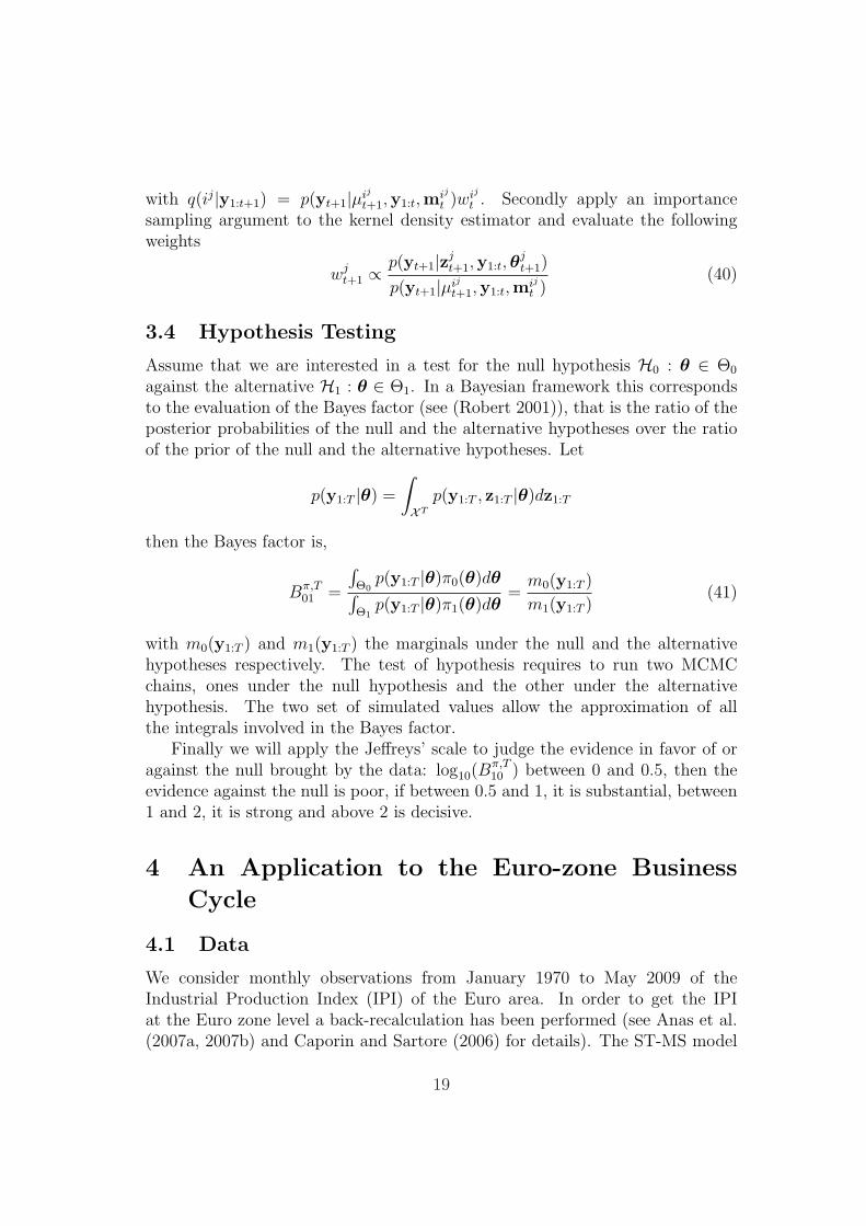
Table 1: First column: estimated parameters for the ST-MS model for the log-change of the Euro Industrial Production Index. Other columns: parameterestimates, 0.025 and 0.975 quantiles, standard deviations (s.d.) and convergencediagnostic statistics (CD). The statistics have been obtained by iterating 5,000times the Gibbs sampler and then discarding the first 1,000 iterations to have aMCMC sample from the stationary distribution.
minimize the parameter estimation bias, due to the regularization step, andavoid the degeneracy problem. We initialized the particle filter with a properlyweighted sample (see Casarin and Marin (2009)) obtained by running the Gibbssampler given in Section 3 on an initial set of observations.
In order to asses the degree of similarity between the three models we considera set of indicators, which are widely used in the literature on business cycleanalysis. First we employ the concordance statistic (C) for regular periodicbehavior in the business cycles proposed by Harding and Pagan (2002). Letsit = I]0.5,1](pt) be the filtered regime at time t, with pit =
∑Nj=1 wj
t I{0}(sjt), for
the three models: CT-MS (i = 1), DT-MS (i = 2) and ST-MS (i = 3). Then theconcordance statistics measures the proportion of time during which two seriessit and sjt, are in the same state. The degree of concordance is then
CijT =
1
T
{T∑
t=1
(sitsjt) + (1− sit)(1− sjt)
}(45)
where T is the sample size. This measure ranges between 0 and 1, with 0representing perfectly counter-cyclical switches, and 1 perfectly synchronous
25
AF CT-MS DT-MS ST-MSAF 1 0.4261 0.6150 0.6223
CT-MS 1 0.3693 0.3681DT-MS 1 0.8750ST-MS 1
β = 0.5Statistics AF vs CT-MS AF vs DT-MS AF vs ST-MSQPST (β) 0.0057 0.0057 0.0057TPST (β) 0.0078 0.0071 0.0063CGoFT (β) 0.0057 0.0057 0.0057RCT (β) 0.0056 0.0057 0.0057
Table 2: Up: degree of concordance {CijT } between the filtered business cycle
phases from our models: CT-MS, DT-MS and ST-MS and the cycle estimatedin Anas et al. (2007b) (AF) for the sample period July 1991-February 2006.Bottom: concordance level measured with QPS, TPS, CGoF and RC statisticsfor the three models and for β = 0.5 with the reference cycle given in Anas etal. (2007b).
shifts. For two regimes described by random walks, the measure will be 0.5in the limit.
We evaluate other criteria based on the following indicator
It = ((1− pit)− pit) (46)
The indicator It is in the [−1, 1] interval. It is close to 1 when the economyis in a recession phase and close to 1 in a expansion phase. Given a thresholdβ ∈ [0, 1], it is possible to define the following decision rule. We will say thatthe economy is a recession phase if It ∈ [−1,−β[ and in an expansion phaseif It ∈ [β, 1]. The threshold β can be estimated empirically and take generallyvalues in the [0.3, 0.5] interval.
The first criteria is the the Quadratic Probabilistic Score (QPS) proposed inBrier (1950).
QPST (β) =1
T
T∑t=1
(I{It<β} − rt
)2(47)
with IA the indicator function, which is 1 if It < β and 0 otherwise and rt thereference cycle given in Anas et al. (2007b). This criterion suffers from thedrawbacks that two non-correlated variables may exhibit a high value of QPS iftheir persistence is strong (Harding and Pagan, 2006). Thus Darne and Ferrara
Figure 6: Left Column: Sequential estimate of the recession probability inthe Euro area (upper charts) and sequentially filtered regimes (bottom charts,st) for model the three MS models. Right Column: Sequential evaluationof QPSi
t(β) = 1t
∑tk=1(I{Iik<β} − rk)
2 and TPSit(β) = 1
t
∑tk=1[1 + (2rk −
1)(arctan(Iikβ)/ arctan(β))] for β = 0.5, t = 1, . . . , T , Iik the recession indicatorresulting from Mi and rk the reference cycle in Anas et al. (2007b) (AF).
(2009) propose the Cyclical Goodness of Fit (CGoF) criterion, defined as
CGoFT (β) =1
T
T∑t=1
[1 + (2rt − 1)(I{It>β} − I{It<−β})
]. (48)
Another indicator is the readability criterion (RC)
RCT (β) =1
T
T∑t=1
I{−β≤It≤β}. (49)
In the regime between expansion and recession phases the signal is difficult tointerpret. Therefore, a readable indicator counts how many times the signalstays in the intermediate zone. Note that QPS and RC are based on step-wisetransform of the signal It which associate a loss equal to 2 to the large errors(out of the interval [−β, β]) and 1 for errors in the interval [−β, β]. It is also
27
possible to introduce a continuously transformed probabilistic score (TPS)
TPST (β) =1
T
T∑t=1
[1 + (2rt − 1)
arctan(βIt)
arctan(β)
], (50)
with β ∈ [0, +∞[. In this indicator a continuous nonlinear function associates aloss level between 2 and 0 to all the errors in the [−1, 1] interval.
The concordance and QPS, TPS, CGoF and RC statistics allow us toconclude that each one of the three models captures different features of therecession phases, when compared to the AF’s cycle. In particular the left columnof Fig. 6 exhibits the sequentially filtered regimes. The outputs of the threemodels differ in terms of numbers of turning points detected in the businesscycle and in terms of phases duration. The concordance and QPS statistics,over the period July 1991 - February 2006, indicates that the regime changesdetected with the ST-MS are similar to the shifts in Anas et al. (2007b) (AF)and have a lower concordance, below 0.4, with the regimes changes detectedwith model CT-MS. The ST-MS and DT-MS have a high degree of concordance(above 0.6) with the reference cycle. The QPS and CGoF statistics (rightcolumn Fig. 6 and Tab. 2) bring us to conclude that the three models seemto be equivalent (CGoF=0.0057, QPS=0.0057), but the TPS, which considers acontinuous weighting function for all the errors in the [−1, 1] interval, indicatesthat the output of the ST-MS model (TPS=0.0063) is more similar to thereference cycle than the regime changes detected with the CT-MS (TPS=0.0078)and DT-MS (TPS=0.0071) models. Fig. 7 evidences the differences between thethree models in detecting the beginning of the last recession period in the sample.
5 Conclusion
We propose a new class of Markov-switching latent factor models with stochastictransition probabilities. This class of models can account for time variationand randomness in the duration of the different regimes. The proposedparameterization has been employed in the context of inference on beta mixtureand on beta regression modelling and allows a straightforward interpretation ofthe model parameters. We suggest an inference procedure based on the Bayesianparadigm and propose a MCMC estimation procedure. Finally, we apply thestochastic transition model and the MCMC estimation framework to the dataof the Euro-zone business cycle and compare the results with exiting datations.
Figure 7: Sequential estimate of the recession periods (i.e. st = 0), with the CT-MS, DT-MS and ST-MS models, for the Euro area during the period January2007 - May 2009.
References
Albert, J. H., and S. Chib (1993): “Bayes inference via Gibbs samplngof autoregressive time series subject to Markov mean and variance shifts,”Journal of Business and Economic Statistics, 11, 1–15.
Anas, J., M. Billio, L. Ferrara, and M. Lo Duca (2007a): “BusinessCycle Analysis with Multivariate Markov Switching Models,” in Growth andCycle in the Eurozone, ed. by G. L. Mazzi, and G. Savio, pp. 249–260. PalgraveMacMillan.
(2007b): “A turning point chronology for the Euro-zone classical andgrowth cycle, in growth and cycle in the Euro-zone,” in Growth and Cyclein the Eurozone, ed. by G. L. Mazzi, and G. Savio, pp. 261–274. PalgraveMacMillan.
Anas, J., M. Billio, L. Ferrara, and G. L. Mazzi (2008): “A Systemfor Dating and Detecting Turning Points in the Euro Area.,” The ManchesterSchool, 76, 549–577.
29
Arulampalam, S., S. Maskell, N. Gordon, and T. Clapp (2001): “ATutorial on Particle Filters for On-line Nonlinear/Non-Gaussian BayesianTracking,” Technical Report, QinetiQ Ltd., DSTO, Cambridge.
Bauwens, L., M. Lubrano, and J. F. Richard (1999): Bayesian Inferencein Dynamic Econometric Models. Oxford University Press, New York.
Berzuini, C., N. G. Best, W. R. Gilks, and C. Larizza (1997): “Dynamicconditional independence models and Markov chain Monte Carlo methods,”Journal of the American Statistical Association, 92, 1403–1441.
Billio, M., and R. Casarin (2009): “Identifying Business Cycle TurningPoints with Sequential Monte Carlo Methods: an Online and Real-TimeApplication to the Euro Area,” Journal of Forecasting, 0, 0–0.
Billio, M., R. Casarin, and D. Sartore (2007): “Bayesian Inference onDynamic Models with Latent Factors,” in Growth and Cycle in the Eurozone,ed. by G. L. Mazzi, and G. Savio, pp. 25–44. Palgrave MacMillan.
Billio, M., A. Monfort, and C. Robert (1999): “Bayesian estimation ofswitching ARMA models,” Journal of Econometrics, 93, 229–255.
Brier, G. W. (1950): “Verification of Forecasts Expressed in Terms ofProbability,” Monthly Weather Review, 75, 1–3.
Caporin, M., and D. Sartore (2006): “Methodological aspects of time seriesback-calculation,” Working Paper, DSE, University of Venice.
Carter, C. K., and R. Kohn (1994): “On Gibbs Sampling for State SpaceModels,” Biometrika, 81, n. 3, 541–553.
Casarin, R., and J.-M. Marin (2009): “Online data processing: Comparisonof Bayesian regularized particle filters,” Electronic Journal of Statistics, 3,239–258.
Chib, S., and E. Greenberg (1995): “Understanding the Metropolis-Hastingsalgorithm,” The American Statistician, 49, 327–335.
Darne, O., and L. Ferrara (2009): “Identification of slowdowns andaccelerations for the euro area economy,” Technical Report, Banque de France.
Diebold, F. X., and G. D. Rudebusch (1996): “Measuring Business Cycles:A Modern Perspective,” The Review of Economics and Statistics, 78, 67–77.
30
Doucet, A., J. G. Freitas, and J. Gordon (2001): Sequential Monte CarloMethods in Practice. Springer Verlag, New York.
Doucet, A., S. Godsill, and C. Andrieu (2000): “On sequential MonteCarlo sampling methods for Bayesian filtering,” Statistics and Computing, 10,197–208.
Durland, J. M., and T. H. McCurdy (1994): “Duration-depedenttransition in Markov model of U.S. GNP growth.,” Journal of Business andEconomics Statistics, 12, 279–288.
Ferrari, S., and F. Cribari-Neto (2004): “Beta regression for modellingrates and proportions,” Journal of Applied Statistics, 31, 799–815.
Filardo, A. F. (1994): “Business Cycle phases and their transitionaldynamics,” Journal of Business and Economics Statistics, 12, 299–308.
Gagliardini, P., and C. Gourieroux (2005): “Stochastic Migration Modelswith Application to Corporate Risk,” Journal of Financial Econometrics, 3,188–226.
Geweke, J. (1992): “Evaluating the accuracy of sampling-based approaches tothe calculation of posterior moments,” in Bayesian Statistics 4, ed. by J. M.Bernardo, J. O. Berger, A. P. Dawid, and A. F. M. Smith, pp. 169–193. OxfordUniversity Press, Oxford.
Goldfeld, S. M., and R. E. Quandt (1973): “A Markov Model forSwitching Regression,” Journal of Econometrics, 1, 3–16.
Hamilton, J. D. (1989): “A new approach to the economic analysis ofnonstationary time series and the business cycle,” Econometrica, 57, 357–384.
Harding, D., and A. Pagan (2002): “Dissecting the Cycle: A MethodologicalInvestigation,” Journal of Monetary Economics, 49, 365–381.
Harrison, J., and M. West (1997): Bayesian Forecasting and DynamicModels, 2nd Ed. Springer Verlag, New York.
Kim, C. J. (1994): “Dynamic linear models with Markov switching,” Journalof Econometrics, 60, 1–22.
Kim, C. J., and C. J. Murray (2001): “Permanent and TransitoryComponents of Recessions,” Empirical Economics, forthcoming.
31
Kim, C. J., and C. R. Nelson (1999a): “Has the U.S. economy becomemore stable? a Bayesian approach based on a Markov-switching model of thebusiness cycle,” Review of Economics and Economic Statistics, 81, 608–616.
(1999b): State-Space Models with Regime Switching. MIT press,Cambridge.
Kim, C. J., and J. Piger (2000): “Common stochastic trends, commoncycles, and asymmetry in economic fluctuations,” Working paper, n. 681,International Finance Division, Federal Reserve Board, Semptember 2000.
Krolzig, H.-M. (1997): Markov Switching Vector Autoregressions. Modelling,Statistical Inference and Application to Business Cycle Analysis. Springer,Berlin.
(2004): “Constructing turning point chronologies with Markov-switching vector autoregressive models: the euro-zone business cycle,” inModern Tools for Business Cycle Analysis, ed. by G. L. Mazzi, and G. Savio,pp. 147–190. Eurostat, Luxembourg.
Liu, J., and M. West (2001): “Combined Parameter and State Estimation inSimulation Based Filtering,” in Sequential Monte Carlo Methods in Practice,ed. by F. J. Doucet A., and G. J., pp. 197–223. Springer-Verlag, New York.
Liu, J. S., W. H. Wong, and A. Kong (1994): “Covariance structure ofthe Gibbs sampler with applications to the comparison of estimators andaugmentation schemes,” Biometrika, 81, 27–40.
Musso, C., N. Oudjane, and F. LeGland (2001): “Improving RegularisedParticle Filters,” in Sequential Monte Carlo in Practice, ed. by F. J. Doucet A.,and G. J., pp. 247–271. Springer Verlag, New York.
Potter, S. M. (1995): “A Nonlinear Approach to U.S. GNP,” Journal ofApplied Econometrics, 10, 109–125.
Robert, C. P. (2001): The Bayesian Choice, 2nd ed. Springer Verlag, NewYork.
Robert, C. P., and G. Casella (1999): Monte Carlo Statistical Methods.Springer Verlag, New York.
Sichel, D. E. (1991): “Business cycle duration dependence: A parametricapproach,” Review of Economics and Statistics, 73, 254–256.
32
Tanner, M., and W. Wong (1987): “The calculation of posteriordistributions by data augmentation,” Journal of the American StatisticalAssociation, 82, 528–550.
Tanner, M. A. (1993): Tools for statistical inference (Lecture Notes inStatistics 67). Springer-Verlag, New York.
Tong, H. (1983): Threshold Models in Non-Linear Time-Series Models.Springer-Verlag, New York.
Watson, J. (1994): “Business cycle durations and postwar stabilization of theu.s. economy,” American Economic Review, 84, 24–46.
33
Discussion Papers recentemente pubblicati Anno 2007 0701 – Sergio VERGALLI “Entry and Exit Strategies in Migration Dynamics” (gennaio) 0702 – Rosella LEVAGGI, Francesco MENONCIN “A note on optimal tax evasion in the presence of merit goods” (marzo) 0703 – Roberto CASARIN, Jean-Michel MARIN “Online data processing: comparison of Bayesian regularized particle filters” (aprile) 0704 – Gianni AMISANO, Oreste TRISTANI “Euro area inflation persistence in an estimated nonlinear DSGE model” (maggio) 0705 – John GEWEKE, Gianni AMISANO “Hierarchical Markov Normal Mixture Models with Applications to Financial Asset Returns” (luglio) 0706 – Gianni AMISANO, Roberto SAVONA “Imperfect Predictability and Mutual Fund Dynamics: How Managers Use Predictors in Changing Systematic Risk” (settembre) 0707 – Laura LEVAGGI, Rosella LEVAGGI “Regulation strategies for public service provision” (ottobre) Anno 2008 0801 – Amedeo FOSSATI, Rosella LEVAGGI “Delay is not the answer: waiting time in health care & income redistribution” (gennaio) 0802 - Mauro GHINAMO, Paolo PANTEGHINI, Federico REVELLI " FDI determination and corporate tax competition in a volatile world" (aprile) 0803 – Vesa KANNIAINEN, Paolo PANTEGHINI “Tax neutrality: Illusion or reality? The case of Entrepreneurship” (maggio) 0804 – Paolo PANTEGHINI “Corporate Debt, Hybrid Securities and the Effective Tax Rate” (luglio) 0805 – Michele MORETTO, Sergio VERGALLI “Managing Migration Through Quotas: an Option-Theory perspective” (luglio) 0806 – Francesco MENONCIN, Paolo PANTEGHINI “The Johansson-Samuelson Theorem in General Equilibrium: A Rebuttal” (luglio) 0807 – Raffaele MINIACI – Sergio PASTORELLO “Mean-variance econometric analysis of household portfolios” (luglio) 0808 – Alessandro BUCCIOL – Raffaele MINIACI “Household portfolios and implicit risk aversion” (luglio) 0809 – Laura PODDI, Sergio VERGALLI “Does corporate social responsability affect firms performance?” (luglio) 0810 – Stefano CAPRI, Rosella LEVAGGI “Drug pricing and risk sarin agreements” (luglio) 0811 – Ola ANDERSSON, Matteo M. GALIZZI, Tim HOPPE, Sebastian KRANZ, Karen VAN DER WIEL, Erik WENGSTROM “Persuasion in Experimental Ultimatum Games” (luglio) 0812 – Rosella LEVAGGI “Decentralisation vs fiscal federalism in the presence of impure public goods” (agosto) 0813 – Federico BIAGI, Maria Laura PARISI, Lucia VERGANO “Organizational Innovations and Labor Productivity in a Panel of Italian Manufacturing Firms” (agosto) 0814 – Gianni AMISANO, Roberto CASARIN “Particle Filters for Markov-Switching Stochastic-Correlation Models” (agosto) 0815 – Monica BILLIO, Roberto CASARIN “Identifying Business Cycle Turning Points with Sequential Monte Carlo Methods” (agosto)
0816 – Roberto CASARIN, Domenico SARTORE “Matrix-State Particle Filter for Wishart Stochastic Volatility Processes” (agosto) 0817 – Roberto CASARIN, Loriana PELIZZON, Andrea PIVA “Italian Equity Funds: Efficiency and Performance Persistence” (settembre) 0818 – Chiara DALLE NOGARE, Matteo GALIZZI “The political economy of cultural spending: evidence from italian cities” (ottobre) Anno 2009 0901 – Alessandra DEL BOCA, Michele FRATIANNI, Franco SPINELLI, Carmine TRECROCI “Wage Bargaining Coordination and the Phillips curve in Italy” (gennaio) 0902 – Laura LEVAGGI, Rosella LEVAGGI “Welfare properties of restrictions to health care services based on cost effectiveness” (marzo) 0903 – Rosella LEVAGGI “From Local to global public goods: how should externalities be represented?” (marzo) 0904 – Paolo PANTEGHINI “On the Equivalence between Labor and Consumption Taxation” (aprile) 0905 – Sandye GLORIA-PALERMO “Les conséquences idéologiques de la crise des subprimes” (aprile) 0906 – Matteo M. GALIZZI "Bargaining and Networks in a Gas Bilateral Oligopoly” (aprile) 0907 – Chiara D’ALPAOS, Michele FRATIANNI, Paola VALBONESI, Sergio VERGALLI “It is never too late”: optimal penalty for investment delay in public procurement contracts (maggio) 0908 – Alessandra DEL BOCA, Michele FRATIANNI, Franco SPINELLI, Carmine TRECROCI “The Phillips Curve and the Italian Lira, 1861-1998” (giugno) 0909 – Rosella LEVAGGI, Francesco MENONCIN “Decentralised provision of merit and impure public goods” (luglio) 0910 – Francesco MENONCIN, Paolo PANTEGHINI “Retrospective Capital Gains Taxation in the Real World” (settembre) 0911 – Alessandro FEDELE, Raffaele MINIACI “Do Social Enterprises Finance Their Investments Differently from For-profit Firms? The Case of Social Residential Services in Italy” (ottobre) 0912 – Alessandro FEDELE, Paolo PANTEGHINI, Sergio VERGALLI “Optimal Investment and Financial Strategies under Tax Rate Uncertainty” (ottobre) 0913 – Alessandro FEDELE, Francesco LIUCCI, Andrea MANTOVANI “Credit Availability in the Crisis: The Case of European Investment Bank Group” (ottobre) 0914 – Paolo BUONANNO, Matteo GALIZZI “Advocatus, et non latro? Testing the Supplier-Induced-Demand Hypothesis for Italian Courts of Justice” (dicembre) 0915 – Alberto BISIN, Jonh GEANAKOPLOS, Piero GOTTARDI, Enrico MINELLI, H. POLEMARCHAKIS “Markets and contracts” (dicembre) 0916 – Jacques H. DRÈZE, Oussama LACHIRI, Enrico MINELLI “Stock Prices, Anticipations and Investment in General Equilibrium” (dicembre) 0917 – Martin MEIER, Enrico MINELLI, Herakles POLEMARCHAKIS “Competitive markets with private information on both sides” (dicembre) Anno 2010 1001 – Eugenio BRENTARI, Rosella LEVAGGI “Hedonic Price for the Italian Red Wine: a Panel Analysis” (gennaio)