Bayesian Filters for Location Estimation and Tracking – An...

Bayesian Filters for Location Estimationand Tracking – An Introduction

Traian E. Abrudan

[email protected] .

Instituto de Telecomunicacoes, Departamento de Engenharia

Electrotecnica e Computadores, Universidade do Porto, Portugal

Bayes filters for location estimation and tracking - GETA Winter School: Short Course on Wireless Localization, Ruka, Feb. 13–15, 2012 p 1

Outline• Motivation• Deterministic vs. probabilistic models• Probabilistic models for location estimation and tracking• Bayesian filters

− Kalman filter and its extensions− Grid-based filter− Particle filter− Pros. and cons.

• Real-world results• Conclusions


Motivation• Many applications require

− estimating parameters that possess certain dynamic behavior

− fusing measurements originating from multiple (different) sensors


Motivation• Indoor propagation environment is extremely harsh

• Signals experience deep fades in space, time and frequency

• As a results of all these effects, the propagation channel behavesrandomly

• Measurements are subject to random errors due to

− random noise at the sensors

− device manufacturing imperfections

− imperfect calibration• Dealing with uncertainties calls for probabilistic models• Powerful statistical estimators may be derived• They do not just provide an estimated value, they also provide

reliability information


Deterministic vs. statistical models• Deterministic models for location estimation are quite “rough”

− perform “hard decisions” (quantize the estimated parameters)− discard valuable statistical information embedded in the data

• Probabilistic models exploit the available statistical information− Parameters are modeled as random variables with the

corresponding probability density functions (p.d.f.’s)− Prior knowledge on the errors (e.g. from the measurements) may

be included in the model in order to improve the parameterestimation

− Optimality can be achieved w.r.t the assumed prior (in somepractical cases just asymptotically)


Probabilistic modelsfor localization and navigation applications

• Let xk denote the LS × 1 true state vector at time instance k, withxk ∈ Dx ⊂ RLS (or CLS )

• xk may include the position (but also velocity, acceleration,heading, etc.)

• Let zk be the observation vector at time k (e.g. measured GPSposition, received signal power, or combinations of those)

• Our goal is to estimate the sequence of states xk, k = 0, 1 . . . ,

based on all available measurements up to time k (abbreviated z1:k)• For this reason, the process is called filtering, and the

corresponding estimators are called Bayesian filters• The posterior p.d.f. we are interested in is p(xk|z1:k)

• Assume that the (hidden) true states xk are connected in a1st-order Markov chain – Hidden Markov Model (HMM)


Probabilistic modelsfor location estimation and tracking

time instance

observations(measurements)

hidden states(cannot be observed and

have to be estimated)

k − 1 k k + 1

xk−1 xk xk+1

zk−1 zkzk+1

p(xk|xk−

1)

p(zk|xk)

Figure 1: First-order Hidden Markov Model [Muh03]

Markov model assumptions:• The current true state is conditionally independent of all previous

states given the last state: p(xk|x1:k−1) = p(xk|xk−1)

• Observations z1:k are conditionally independent provided thatx0, . . . ,xk, are known: p(zk|x1:k) = p(zk|xk)


Probabilistic models – State-space model

prediction equation: xk = f(xk−1,uk) + wk

measurement equation: zk = h(xk) + vk

→ p(xk|xk−1)

→ p(zk|xk)

(1)

(2)

f ,h are known functionsuk is a known input (required only if a control input exists)wk is the state (process) noisevk is the measurement noisewk,vk are i.i.d., mutually independent, with known p.d.f.’s

• prediction equation: dynamic model of the system that describesthe mutual dependence of the true states we would like to estimate(for localization, this corresponds to a motion model)

• measurement equation: a model for the sensor(s) that describeshow observations are related to the true states (e.g. RSSI, ToA,AoA, kinematic parameters, etc., or combinations)


Probabilistic models – State-space model

prediction equation: xk = f(xk−1,uk) + wk

measurement equation: zk = h(xk) + vk

→ p(xk|xk−1)

→ p(zk|xk)

(3)

(4)

• Question What to trust more: the prediction or the measurement?• The Bayesian estimator solves this problem reliably using a

predict-update mechanism

• We would like to derive a formula such that the new posterior p.d.f.at time k, p(xk|z1:k) is obtained by updating the old posterior attime k − 1, p(xk−1|z1:k−1)

• This way, the filter can operate sequentially, in real-time (online)• Moreover, we store only the parameters at the previous time

instance and avoid memory growth



• Assume that the old posterior p(xk−1|z1:k−1) is available at time k

• Prediction step: p(xk−1|z1:k−1) → p(xk|z1:k−1)

• Using Chapman-Kolmogorov equation:

p(xk|z1:k−1) =

∫

Dx

p(xk|xk−1)p(xk−1|z1:k−1)dxk−1 (5)

• This is the prior of the state xk without knowing the incomingmeasurement zk, knowing only the previous measurements z1:k−1

• The prediction step usually deforms / translates / spreads the p.d.f.due to noise



• Update step:{p(xk|z1:k−1), zk

}→ p(xk|z1:k)

p(xk|z1:k) =p(zk|xk)p(xk|z1:k−1)

p(zk|z1:k−1), i.e., posterior =

likelihood · priorevidence

(6)

• The denominator c = p(zk|z1:k−1) =∫

Dx

p(zk|xk)p(xk|z1:k−1)dxk isjust a normalization constant (independent of xk)

• The update combines the likelihood of the received measurementwith the predicted state

• The update step usually concentrates the p.d.f.• A closed-form expression that relates the old posterior to the new

posterior is obtained by replacing eq. (5) into eq. (6)



• Sequential update of the posterior p(xk−1|z1:k−1), zk → p(xk|z1:k):

p(xk|z1:k)︸︷︷︸

posterior at time k

=1

cp(zk|xk)︸︷︷︸

from meas. eq.

∫

Dx

p(xk|xk−1)︸︷︷︸

from pred. eq.

p(xk−1|z1:k−1)︸︷︷︸

posterior at time k−1

dxk−1 (7)

• This theoretically allows an optimal Bayesian solution – MinimumMean Square Error (MMSE), Maximum a posteriori (MAP)estimators, etc.

• Unfortunately, this is just a conceptual solution, integrals areintractable

• In some cases (under restrictive assumptions), (close to) optimaltractable solutions are obtained:− Kalman filter [Sin70, ParLee01, AbrPauBar11]− grid-based filter [Muh03]


Kalman filter (KF)• State-space model:

prediction equation: xk = Fkxk−1 + Bkuk + Gkwk

measurement equation: zk = Hkxk + vk

(8)

(9)

where Fk,Bk,Gk,Hk are known matrices• When noises are zero-mean jointly Gaussian, Kalman filter is

optimal estimator in the mean-square error (MSE) sense• Otherwise, KF is the best linear estimator• It finds the posterior mean E{xk|z1:k} = xk|k and its covariance

E{(xk − xk|k)(xk − xk|k)T } and updates them sequentially

xk|k = xk|k−1 − Kk[zk − Fkxk|k−1] (10)

where Kk is the Kalman gain, and the subscript (·)k|k−1 denotes thea priori estimated state (before considering the measurement zk)


Kalman filter and its extensions (EKF, UKF)• Extended Kalman filter (EKF) – an extension of KF to non-linear

state-space equations− either the process is non-linear, or the measurements are not a

linear function of the states− EKF linearizes the model about the new estimate (similar to

Taylor series approximation)− works well in many situations, but may diverge for highly

non-linear models (covariance is propagated throughlinearization)

• Unscented Kalman filter (UKF) – mean and covariance areprojected via the so-called unscented transform− picks up a minimal set of sample points around the mean –

called sigma points – propagates those through the non-linearity− UKF can deal with highly-nonlinear models− often, UKF works better than EKF


Kalman filter and its extensions (EKF, UKF)• KF, EKF, UKF do not work very well for p.d.f.’s that have

− heavy-tails / high kurtosis• They may totally fail for

− heavily skewed p.d.f.’s− bimodal/multimodal p.d.f.’s

• We need more general filters to tackle these problems• It is everything about approximating well integrals and the p.d.f.’s in

the optimal Bayes estimation of the posterior

p(xk|z1:k)︸︷︷︸

posterior at time k

=1

cp(zk|xk)︸︷︷︸

from meas. eq.

∫

Dx

p(xk|xk−1)︸︷︷︸

from pred. eq.

p(xk−1|z1:k−1)︸︷︷︸

posterior at time k−1

dxk−1

• The price we pay is the high complexity – curse of dimensionality[DauHua03]


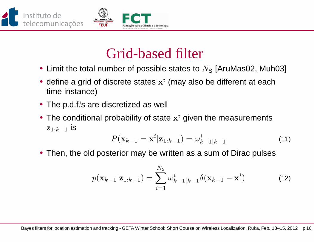
Grid-based filter• Limit the total number of possible states to NS [AruMas02, Muh03]• define a grid of discrete states xi (may also be different at each

time instance)• The p.d.f.’s are discretized as well• The conditional probability of state xi given the measurements

z1:k−1 isP (xk−1 = xi|z1:k−1) = ωi

k−1|k−1 (11)

• Then, the old posterior may be written as a sum of Dirac pulses

p(xk−1|z1:k−1) =

NS∑

i=1

ωik−1|k−1δ(xk−1 − xi) (12)


Grid-based filter

• Both the new prior and the new posterior have the same structure:a sum of weighted and delayed Dirac impulses

p(xk|z1:k−1) =

NS∑

i=1

ωik|k−1δ(xk−1 − xi) (13)

p(xk|z1:k) =

NS∑

i=1

ωik|kδ(xk−1 − xi) (14)


Grid-based filter• The prediction step: the Chapman-Kolmogorov equation for the

prior (5) becomes:

p(xk|z1:k−1) =

NS∑

i=1

NS∑

j=1

ωj

k−1|k−1p(xi|xj)δ(xk−1 − xi) (15)

=

NS∑

i=1

ωik|k−1δ(xk−1 − xi) (16)

where

ωik|k−1 =

NS∑

j=1

ωj

k−1|k−1p(xi|xj) (17)

new prior weights = old posterior weights, reweighted using

state transition probabilities


Grid-based filter• The update step: equation (6) becomes:

p(xk|z1:k) =

NS∑

i=1

ωik|kδ(xk−1 − xi) (18)

where

ωik|k =

ωik|k−1p(zk|xi)

∑NSj=1 ω

j

k|k−1p(zk|xj)(19)

posterior weights = prior weights, reweighted using likelihoods

• Grid-based filters are computationally expensive• Grid resolution needs to be sufficiently high


Particle filter• Particle filters are sophisticated estimation techniques based on

simulation• Also known as Sequential Monte Carlo (SMC) methods

[GusGun02, AruMas02, Muh03, Kar05, Ber99]• Integrals involved in the Bayesian filter cannot be solved analytically• The idea: represent the p.d.f.’s by using a set of random “particles”

(random = Monte Carlo method)• Particles are just differently weighted samples of the distribution• By increasing the number of samples, the representation almost

sure converges to the true p.d.f.


Particle filter

−3 −2 −1 0 1 2 3 4 5−0.1

0

0.1

0.2

0.3

0.4

0.5

0.6equal weight particles

−3 −2 −1 0 1 2 3 4 5−0.1

0

0.1

0.2

0.3

0.4

0.5

0.6non−equal weight particles

original p.d.f.representatation of the p.d.f.

original p.d.f.representatation of the p.d.f.

Figure 2: Representation of the Gaussian p.d.f. N (1, 1) using particles(1-D case). The particle weight is represented by its size.


Particle filter

−4−2

02

4

−4−2

02

40

0.05

0.1

0.15

0.2

2−D Gaussian p.d.f. equal weight particles

−4 −2 0 2 4−4

−3

−2

−1

0

1

2

3

4non−equal weight particles

−4 −2 0 2 4−4

−3

−2

−1

0

1

2

3

4

Figure 3: Representation of the Gaussian p.d.f. using particles (1-Dcase). The particle weight is represented by its size. The p.d.f. isN ([0.5; 1], [1.6 0.8; 0.8 0.8])


Particle filterSequential Importance Sampling (SIS)

• SIS is the basic framework for most particle filter algorithms• Let {xi

0:k} be a set of points (particles), i = 1, . . . , NP

• This describes the whole trajectory in the state space for eachparticle i

• Let ωik be the associated weights, normalized such that

∑NP

i=1 ωik = 1

• Then, the discrete weighted approximation of the posterior p.d.f. is

p(xk|z1:k) ≈NP∑

i=1

ωikδ(x0:k − xi

0:k) (20)



• Usually, we cannot draw samples xik from p(·) directly

• Assume we sample directly for a (different) importance density q(·)

• Our approximation is still correct (up to normalization) if

ωik ∝

p(xi0:k|z1:k)

q(xi0:k|z1:k)

(21)

• The benefit is that we can choose q(·) freely• If the importance function is chosen to factorize such that

q(x0:k|z1:k) = q(xk|x0:k−1, z1:k)q(x0:k−1|z1:k−1) (22)

then one can augment the old particles xi0:k−1 by

xk ∼ q(xk|x0:k−1, z1:k) to get the new particles xi0:k



• The weight update is of form

ωik = ωi

k−1

p(zk|xik)p(xi

k|xik−1)

q(xik|x0:k−1, z1:k)

(23)

• Furthermore, if q(xik|x0:k−1, z1:k) = q(xi

k|xk−1, z1:k) (onlydependent on the last state), then we do not need to preserve thefull trajectory of the particles x0:k−1, neither the observations z1:k


Particle filterDegeneracy Problem

• The problem with SIS approach is that after few iterations, mostparticles have negligible weight

• The weight is concentrated on only few particles – the one thatclosely match the measurements

• Solutions:− brute force: huge number of particles – too complex− good choice of importance density− resampling


Particle filterOptimal importance density

• It can be shown that the optimal importance density is given by

qopt(xk|xk−1, zk) = p(xk|xk−1, zk) (24)

• Then

ωik = ωi

k−1

∫

Dx

p(zk|x′k)p(x′

k|xik−1)dx

′k (25)

• Drawing sample from the optimal distribution is not always possible• One alternative is to choose the importance density to be the prior

q(xk|xk−1, zk) = p(xk|xk−1) (26)

• This is simple, but does not take into account the measurements


Particle filterResampling

• Basic idea of resampling:

Whenever the degeneracy exceeds some threshold, replace the

old samples (+ weights) with a new set of samples (+ weights),

such that the sample density reflects better the posterior p.d.f.

• This eliminates particles with low weights and chooses newparticles in the more probable regions

• Complexity is possible in O(NP)


Particle filterResampling

resampling

prediction

step

measurement

& update

old posterior p.d.f.

new posterior p.d.f.

Figure 4: Illustration of the resampling process.


Particle filterPseudo-code [Muh03, AruMas02]

[{xik, ωi

k}NP

i=1] = PF({xik−1, ω

ik−1}

NP

i=1, zik)

FOR i = 1 to NP

draw xik ∼ q(xk|xi

k−1, zk)

update weights according to

ωik = ωi

k−1

p(zk|xik)p(xi

k|xik−1)

q(xik|x0:k−1, z1:k)

END FORnormalize weights to

∑NP

i=1 ωik = 1

IF degeneracy is too high

resample {xik, ωi

k}NP

i=1

END IF• Knowledge of the initial posterior is required – not possible, a

proposal density is usedBayes filters for location estimation and tracking - GETA Winter School: Short Course on Wireless Localization, Ruka, Feb. 13–15, 2012 p 30

Particle filterSample Impoverishment Problem

• No degeneracy problem, but new problem arises• Particle with too high weight are selected more and more often• The other ones will slowly die out• This leads to a loss of diversity or sample impoverishment• For small process noise, all particles can collapse into a single

point within a few iterations• Another problem: resampling limits the possibility to parallelize the

algorithm


Particle filter• There are various other kinds of particle filters in the literature

− sampling importance resampling− auxiliary sampling importance resampling− marginalized (or “Rao-Blackwelized”) particle filter− Gaussian sum particle filter− kernel density estimation based− ...

• There are also Markov Chain Monte Carlo (MCMC) batch Bayesianmethods

• They model the full posterior xk ∼ p(x0, . . . ,xk|yk, . . . ,y0) – notonline, very complex


Bayesian filtersPros. and cons.

✔ close to optimal performance

✔ can deal with non-linearities, non-Gaussian noise – evenmultimodal distributions are not a problem

✔ PF can be implemented in O(NP), mostly parallelizable

✔ in contrast to HMM filters (state space discretized to NS) states, PFfocus on probable regions of the state space

✔ Bayesian filters can reliably fuse data originating from differentsensors (e.g. RF signals, kinematic sensors, cameras, etc.)

✔ As long as the sources of measurement error (randomness) areindependent, fusing multiple sensors will always improve results

✘ might be too complex for some real-time applications

✘ degeneracy and sample impoverishment problems may arise

✘ choosing the importance density might be hard


Bayesian Filters

Thesis: “If you want to solve a problem, particle filters are the best

filters you can use, much better than e.g. Kalman filters.”

• Right or wrong?• Very wrong!• PF contain randomness – only converge to the true posterior when

number of particles NP → ∞ (asymptotically optimal)• If assumption for Kalman filters or grid-based filters hold, no particle

filter can outperform them• In case these assumptions hold approximately, other filters may

perform reasonably well with much lower complexity than PF• For location estimation and tracking, these assumptions do not

hold, in general (multimodal p.d.f’s arise easily)


Practical aspects for localizationMotion model

• It is important to have an accurate description of the reality• People’s motion is subject to physical constraints

− position (accessible areas, transition between them)− speed (stopped, walking, running)− acceleration (changes in speed are limited)

• It is sensible to take into account these constraints when doingposition tracking

• Motion models predict the next position based on the previous one• Information about the building layout may be used as well• Such information may improve drastically the location estimation

and tracking• There are many motion models in the literature: uniform linear

motion, diffusion approach, angular p.d.f., multi-user motionmodels, etc. [AbrPauBar11, Roy11, KaiKhi11, QuiSta10]


Real-world resultsWork in Progress...

• We test a grid-based filter using real-world results, the same as in[AbrPauBar11]

• The sensor nodes are equipped with two RF front-ends operatingat 433MHz and 2.4GHz, respectively

• RSSI on both frequency was used• no knowledge about the building geometry• unknown starting point (initial posterior based on the first

measurement)• the same linear motion model as in [AbrPauBar11]• the true position was measured using a laser range meter



A1 A2

A3A4 starting point1

8

18

ending point25

West−East axis [meters]

Sou

th−

Nor

th a

xis

[met

ers]

Indoor location estimation and tracking

0 2 4 6 8 10

0

1

2

3

4

5

6

7

8

9

10

Figure 5: Location estimation and tracking

• office environment in Aveiro• grid-based filter• spatial grid resolution: 0.5 meters• single user case (for better

visualization)• also because of limited amount of

measurement data• true user path – gray solid line with

circle markers• anchor nodes: A1, . . . ,A4



A1 A2


8

18

ending point25


Sou

th−

Nor

th a

xis

[met

ers]

p(x1 | r

1:1)

0 2 4 6 8 10

0

1

2

3

4

5

6

7

8

9

10


• Receive the very firstmeasurement z1

• initial (proposal) posteriordistribution p(x1|z1:1) – continuousrepresentation

• computed just using the first mea-surement z1



A1 A2


8

18

ending point25


Sou

th−

Nor

th a

xis

[met

ers]

p(x2 | r

1:1)

0 2 4 6 8 10

0

1

2

3

4

5

6

7

8

9

10


• Prediction step – get the prior:

p(x2|z1:1) =

∫

Dx

p(x2|x1)p(x1|z1:1)dx

− p(x2|x1): based on theprediction equation

− p(x1|z1:1): the old posterior• The spreading of the posterior after

the prediction step may be noticed



A1 A2


8

18

ending point25


Sou

th−

Nor

th a

xis

[met

ers]

p(x2 | r

1:1) x p(r

2 | x

2)

0 2 4 6 8 10

0

1

2

3

4

5

6

7

8

9

10


• receive new measurement z2

• Compute its likelihood p(z2|x2)based on the measurementequation (log-distance RSSIchannel model)

• Multiply the likelihood with the priorp(x2|z1:1) and normalize to get thenew posterior



A1 A2


8

18

ending point25


Sou

th−

Nor

th a

xis

[met

ers]

p(x2 | r

1:2)

0 2 4 6 8 10

0

1

2

3

4

5

6

7

8

9

10


• New posterior

p(x2|z1:2) =p(z2|x2)p(x2|z1:1)

p(z2|z1:1)

• The denominator is just anormalization factor – it does notneed to be calculated

• Shrinking of the new posterior mabe noticed

• Calculate new position estimate x

as the dominant mode (maximumposteriori estimate)



A1 A2


8

18

ending point25


Sou

th−

Nor

th a

xis

[met

ers]

xest

(2) vs. xtrue

(2)

0 2 4 6 8 10

0

1

2

3

4

5

6

7

8

9

10


• The estimated (red line) vs. thetrue position (gray line)

• Progress is shown by the orangeline

• Repeat this procedure at everstep...



A1 A2


8

18

ending point25


Sou

th−

Nor

th a

xis

[met

ers]

p(x3 | r

1:2)

0 2 4 6 8 10

0

1

2

3

4

5

6

7

8

9

10


• Prediction: p(x3|z1:2)



A1 A2


8

18

ending point25


Sou

th−

Nor

th a

xis

[met

ers]

p(x3 | r

1:2) x p(r

3 | x

3)

0 2 4 6 8 10

0

1

2

3

4

5

6

7

8

9

10


• New measurement and its likeli-hood p(z3|z3) to be multiplied withthe prior



A1 A2


8

18

ending point25


Sou

th−

Nor

th a

xis

[met

ers]

p(x3 | r

1:3)

0 2 4 6 8 10

0

1

2

3

4

5

6

7

8

9

10


• New posterior p(x3|z1:3)



A1 A2


8

18

ending point25


Sou

th−

Nor

th a

xis

[met

ers]

xest

(3) vs. xtrue

(3)

0 2 4 6 8 10

0

1

2

3

4

5

6

7

8

9

10


• New position estimate x3

• and so on...



A1 A2


8

18

ending point25


Sou

th−

Nor

th a

xis

[met

ers]

xest

(25) vs. xtrue

(25)

0 2 4 6 8 10

0

1

2

3

4

5

6

7

8

9

10


• Tracked location (red solid line withcircle markers)



A1 A2


8

18

ending point25


Sou

th−

Nor

th a

xis

[met

ers]

xest

(25) vs. xtrue

(25)

0 2 4 6 8 10

0

1

2

3

4

5

6

7

8

9

10


• The discretized position estimates


Conclusions• Bayesian filters represent powerful tools for location estimation and

tracking

• They are able to reliably fuse information originating from multiple(possibly different kind) of sensors

• Various approaches exist (KF, EKF, UKF, grid-based filter, particlefilters...)

• They have different degrees complexity/accuracy

• There is no “best option”, the choice depends on the application athand


References[AbrPauBar11] T. E. Abrudan, L. M. Paula, J. Barros, J. P. S. Cunha, and N. B. Carvalho, “Indoor Location

Estimation and Tracking in Wireless Sensor Networks using a Dual Frequency Approach”, 2011IEEE International Conference on Indoor Positioning and Indoor Navigation (IPIN), Guimarães,Portugal, 21–23 Sep. 2011.

[Sin70] R. A. Singer, “Estimating optimal tracking filter performance for manned maneuvering targets”,IEEE Transactions on Aerospace and Electronic Systems, vol. AES-6, pp. 473–483, Jul. 1970.

[ParLee01] S.-T. Park and J. G. Lee, “Improved Kalman filter design for three-dimensional radar tracking”,IEEE Transactions on Aerospace and Electronic Systems, vol. 37, pp. 727–739, Apr. 2001.

[Muh03] Matthias Mühlich, “Particle filters. An overview”, (tutorial presentation), Filter workshop,Bucharest, Romania, 2003.

[AruMas02] M.S. Arulampalam, S. Maskell, N. Gordon, T.Clapp, “A tutorial on particle filters for onlinenonlinear/non-Gaussian Bayesian tracking”, IEEE Transactions on Signal Processing, vol.50,no.2, pp. 174–188, Feb 2002.

[GusGun02] F. Gustafsson, F. Gunnarsson, N. Bergman, U. Forssell, J. Jansson, R. Karlsson, P.-J. Nordlund,“Particle filters for positioning navigation and tracking”, IEEE Transactions on Signal Processing,vol.50, no.2, pp. 425–437, Feb 2002.

[DouFre02] A. Doucet, N. de Freitas, N. Gordon (Eds.), Sequential Monte Carlo Methods in Practice,Springer Verlag, 2001.


References[FoxHig03] V. Fox, J. Hightower, Lin Liao, D. Schulz, G. Borriello, “Bayesian filtering for location estimation”,

IEEE Pervasive Computing, vol.2, no.3, pp. 24–33, Jul.-Sept. 2003.

[DauHua03] F. Daum, J. Huang, “Curse of dimensionality and particle filters,” Proceedings of the IEEEAerospace Conference, 2003, vol.4, no., pp. 4-1979–4-1993, Mar. 8–15, 2003.

[DouJoh09] A. Doucet and A.M. Johansen, “A tutorial on particle filtering and smoothing: fifteen years later”,The Oxford Handbook of Nonlinear Filtering, Oxford University Press, 2009.

[Hau05] A.J. Haug, “A Tutorial on Bayesian Estimation and Tracking Techniques Applicable to Nonlinearand Non-Gaussian Processes”, Mitre Corporation Technical Report, MTR 05W0000004 (publicrelease), Jan. 2005

[CarDav07] F. Caron, M. Davy, E. Duflos, P. Vanheeghe, “Particle filtering for multiuser data fusion withswitching observation models: Applications to land vehicle navigation”, IEEE Transactions onSignal Processing, vol.50, no.2, pp. 425–437, Feb 2002.

[HueCad02] C. Hue, J.-P. Le Cadre, P. Pérez, “Sequential Monte Carlo Methods for Multiple Target Trackingand Data Fusion”, IEEE Transactions on Signal Processing, vol.50, no.2, pp. 309–325, Feb2002.

[HenKar10] G. Hendeby, R. Karlsson, F. Gustafsson, “The Rao-Blackwellized Particle Filter: A Filter BankImplementation” EURASIP Journal on Advances in Signal Processing. vol. 2010, Article ID724087, 10 pages, 2010.


References[SchGusNor05] T. B. Schön, F. Gustafsson and P.-J. Nordlund, “Marginalized particle filters for mixed

linear/nonlinear state-space models”, IEEE Transactions on Signal Processing, vol. 53, no. 7,pp. 2279–2289, Jul. 2005.

[Ber97] N. Bergman, “Bayesian Inference in Terrain Navigation”, Department of Electrical Engineering,Linköping University, Linköping Studies in Science and Technology. Licentiate Thesis No. 649,Nov.1997.

[Ber99] N. Bergman, “Recursive Bayesian Estimation”, Department of Electrical Engineering, LinköpingUniversity, Linköping Studies in Science and Technology. Doctoral dissertation No. 579, 1999.

[Kar05] R. Karlsson, “Particle Filtering”, Department of Electrical Engineering, Linköping University,Linköping Studies in Science and Technology. Doctoral dissertation No. 924, 1999.

[Roy11] R. R. Roy, Handbook of Mobility Models and Mobile Ad Hoc Networks, Springer, 2011.

[QuiSta10] M. Quigley, D. Stavens, A. Coates, and S. Thrun. “Sub-Meter Indoor Localization in UnmodifiedEnvironments with Inexpensive Sensors.” In Proceedings of the IEEE/RSJ InternationalConference on Intelligent Robots and Systems 2010 (IROS10), Taipei, Taiwan, 2010.

[KaiKhi11] S. Kaiser, M. Khider, and P. Robertson, “A maps-based angular PDF for navigation systems inindoor and outdoor environments”, 2011 IEEE International Conference on Indoor Positioningand Indoor Navigation (IPIN), Guimarães, Portugal, 21–23 Sep. 2011.


Date post:	19-Apr-2018
Category:	Documents
Upload:	trannhan
View:	216 times
Download:	3 times

Bayesian Filters for Location Estimation and Tracking – An...

Documents