Chapter 1 Bayesian Inference (09/17/17) A witness with no historical knowledge There is a town where cabs come in two colors, yellow and red. 1 Ninety percent of the cabs are yellow. One night, a taxi hits a pedestrian and leaves the scene without stopping. The skills and the ethics of the driver do not depend on the color of the cab. An out-of-town witness claims that the color of the taxi was red. The out-of town witness does not know the proportion of yellow and red cabs in the town and makes a report on the sole basis of what he thinks he has seen. Since the accident occurred during the night, the witness is not completely reliable but it has been assessed that such a witness makes a correct statement is four out of five (whether the true color of the cab is yellow or red). How should one use the information of the witness? Because of the uncertainty, we should formulate our conclusion in terms of probabilities. Is it more likely then that a red cab was involved in the accident? Although the witness reports red and is correct 80 percent of the time, the answer is no. Recall that there are many more yellow cabs. The red sighting can be explained either by a yellow cab hitting the pedestrian (an event with high prior probability) which is incorrectly identified (an event with low probability), or a red cab (with low probability) which is correctly identified (with high probability). Both the prior probability of the event and the precision of the signal have to be used in the evaluation of the signal. Bayes’ rule 1 The example is adapted from Salop (1987) 1
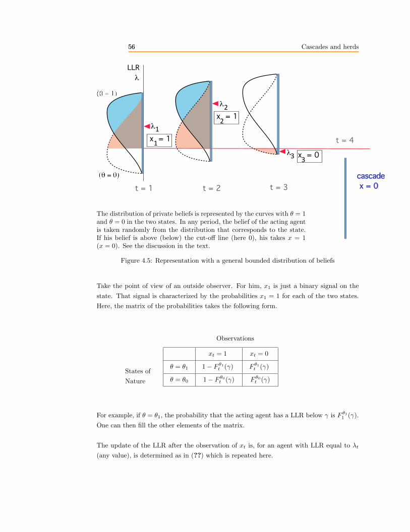
Transcript
Chapter 1
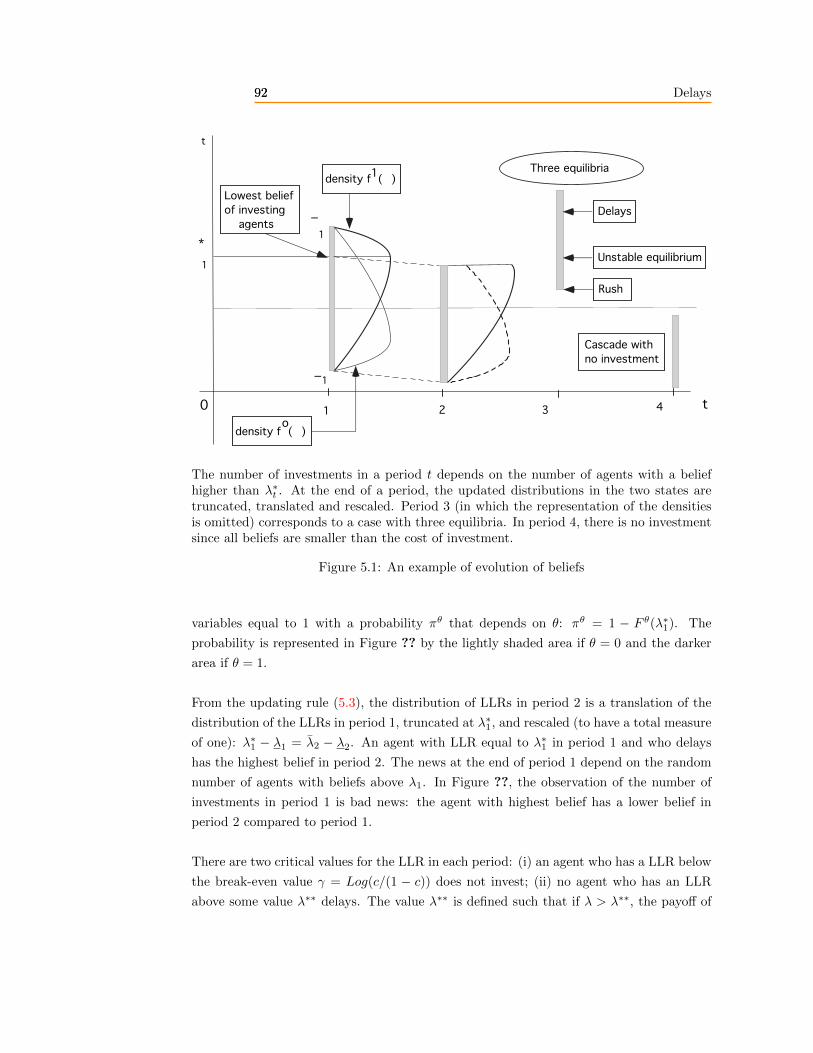
Bayesian Inference
(09/17/17)
A witness with no historical knowledge
There is a town where cabs come in two colors, yellow and red.1 Ninety percent of the cabs
are yellow. One night, a taxi hits a pedestrian and leaves the scene without stopping. The
skills and the ethics of the driver do not depend on the color of the cab. An out-of-town
witness claims that the color of the taxi was red. The out-of town witness does not know
the proportion of yellow and red cabs in the town and makes a report on the sole basis of
what he thinks he has seen. Since the accident occurred during the night, the witness is not
completely reliable but it has been assessed that such a witness makes a correct statement
is four out of five (whether the true color of the cab is yellow or red). How should one
use the information of the witness? Because of the uncertainty, we should formulate our
conclusion in terms of probabilities. Is it more likely then that a red cab was involved in
the accident? Although the witness reports red and is correct 80 percent of the time, the
answer is no.
Recall that there are many more yellow cabs. The red sighting can be explained either
by a yellow cab hitting the pedestrian (an event with high prior probability) which is
incorrectly identified (an event with low probability), or a red cab (with low probability)
which is correctly identified (with high probability). Both the prior probability of the event
and the precision of the signal have to be used in the evaluation of the signal. Bayes’ rule
1The example is adapted from Salop (1987)
1
2 Bayesian tools2
provides the method to compute probability updates. Let R be the event “a red cab is
involved”, and Y the event “a yellow cab is involved”. Likewise, let r (y) be the report “I
have seen a red (yellow) cab”. The probability of the event R conditional on the report r
is denoted by P (R|r). By Bayes’ rule,2
P (R|r) =P (r|R)P (R)
P (r)=
P (r|R)P (R)
P (r|R)P (R) + P (r|Y)(1− P (R)). (1.1)
The probability that a red cab is involved before hearing the testimony is P (R) = 0.10.
P (r|R) is the probability of a correct identification and is equal to 0.8. P (r|Y) is the
probability of an incorrect identification and is equal to 0.2. Hence,
P (R|r) =0.8× 0.1
0.8× 0.1 + 0.2× 0.9=
4
13<
1
2.
Note that this probability is much less than the precision of the witness, 80 percent, because
a “red” observation is more likely to come from a wrong identification of a yellow cab than
from a correct identification of a red cab.
The example reminds us of the difficulties that some people may have in practical cir-
cumstances. Despite these difficulties,3 all rational agents in this book are assumed to be
Bayesians. The book will concentrate only on the difficulties of learning from others by
rational agents.
A witness with historical knowledge
Suppose now that the witness is a resident of the town who knows that only 10 percent of
the cabs are red. In making his report, he tells the color which is the most likely according
to his rational deduction. If he applies the Bayesian rule and knows his probability of
making a mistake, he knows that a yellow cab is more likely to be involved. He will report
“yellow” even if he thinks that he has seen a red cab. If he thinks he has seen a yellow
one, he will also say “yellow”. His private information (the color he thinks he has seen) is
ignored in his report.
The omission of the witness’ information in his report does not matter if he is the only
witness and if the recipient of the report attempts to assess the most likely event: the
witness and the recipient of the report come to the same conclusion. But suppose there is
a second witness with the same sighting skill (correct 80 percent of the time) and who also
thinks he has seen a red cab. That witness who attempts to report the most likely event
2Using the definition of conditional probabilities, P (R|r)P (r) = P (R and r) = P (r|R)P (R).3The ability of people to use Bayes’ rule has been tested in experiments, with mixed results (Holt and
Anderson, 1993).
3 Bayesian tools3
says also “yellow”. The recipient of the two reports learns nothing from the reports. For
him the accident was caused by a yellow cab with a probability of 90 percent.
Recall that when the first witness came from out-of-town, he was not informed about the
local history and he gave an informative report, “red”. That report may be inaccurate,
but it provides information. Furthermore, it triggers more information from the second
witness. After the report of the first witness, the probability of R increased from 0.1 to
4/13. When that probability of 4/13 is conveyed to the second witness, he thinks that a
red car is more likely.4 He therefore reports “red”. The probability of the inspector who
hears the reports of the two witnesses is now raised to the level of the last (second) witness.
Looking for your phone as a Bayesian
You live in a two room apartment with two rooms, one that you keep orderly, one that
is messy. After stepped out with a friend, you realize that you have left your cell phone
behind. The phone is equally likely to be in one of the two rooms. You tell your friend:
please looking for my phone that I have left in the apartment while I fetch the car that is
parked in the next block. Your friend comes back without having found the phone. Which
room is the more probable for the phone. Answer before reading the next paragraph.
You may think that your friend has looked into the two rooms. In the orderly room, it is
harder to miss the phone. Therefore, no seeing the phone in that room makes it unlikely
(compared to the other room) that the phone is there. You increase the probability of the
messy room. You are a Bayesian.
In the formalization of this story, we can that there are two rooms 1 (orderly) and 2
(messy). There are two states of the nature: the phone is in room 1 or room 2. A search
in room i, i = 1 or 2 produces a signal that is 1 (finding the phone) or 0 (not finding the
phone. Each signal has a probability qi to be equal to 1 if the phone is in room i. The
probability of not finding the phone in room i when the phone is actually in room i is
1 − qi is positive. If the phone is in room 3 − i, (the room other than i), the signal si is
zero. When you do not find the phone in Room 1, you think, rationally, you increase your
probability that the phone is in Room 2. If you search in Room 2 for about the same time,
then you think that the probability of a mistaken signal s2 = 0 is higher than s1 = 0 if the
phone is in Room 1. Comparing the two rooms, you increase the probability of the phone
in Room 2. The precise Bayesian calculus will be done later in this chapter.
4Exercise: prove it.
4 Bayesian tools4
1.1 The standard Bayesian model
1.1.1 General remarks
The main issue is to learn about something. In the Bayesian framework, the “something”
is a possible fact, which can be called a state of nature. That fact may take place in the
future or it may already have taken place with an uncertain knowledge about it. Actually,
in a Bayesian framework, there is no difference between a future event and a past event
that are both uncertain. The future event may be “rain” or “shine”, to occur tomorrow.
For a Bayesian, nature chooses the weather today (with some probability, to be described
below), and that weather is realized tomorrow.
The list of possible states is fixed in Bayesian learning. There is no room for learning about
states that are not on the list of possible states before the learning process. That is an
important limitation of Bayesian learning. There is no ”unknown unknown”, to use the
famous characterization of secretary of state Rumsfeld, only “known unknown”. In other
words, one knows what is unknown.
The Bayesian process begins by putting weights on the unknowns, probabilities on the
possible states of nature. These probabilities may be objective, such as the probability of
“tail” or “face” in throwing a coin, but that is not important. What matters is that these
probabilities are the ones that the learner uses at the learning process. These probabilities
will be called belief. A “belief” will be a distribution of probabilities over the possible
states. By an abuse of language, a belief will sometimes be the probability of a particular
state, especially in the case of two possible states: the “belief” in one state will obviously
define the probability of the other state. The belief before the reception of information is
called the prior belief.
Learning is the processing of information that comes about the state. This information
comes in the form of a signal. Examples are the witness report of the previous section, a
weather forecast, an advice by a financial advisor, the action of some “other” individual,
etc... In order to be informative, that signal must depend on the state. But that signal is
imperfect and does not reveal exactly the state (otherwise there would be nothing inter-
esting to think about). A natural definition of a signal is therefore a random variable that
can take different values with some probabilities and the distribution of these probabilities
depend on the actual state. The processing of the information of the signal is the use of
the signal to update the prior belief into the posterior belief. That step is the core of the
Bayesian learning process and its mechanics are driven by Bayes’ rule. In that process,
the learner knows the mechanics of the signal, i.e., the probability of receiving a particular
signal value conditional on the true state. Bayes’ rule combines that knowledge with the
5 Bayesian tools5
prior distribution of the state to compute the posterior distribution.
Examples
1. The binary model
• States of nature θ ∈ Θ = 0, 1
• Signal s ∈ 0, 1 with P (s = θ|θ) = qθ.
2. Financial advising (i.e., Value Line):
• States of nature: a stock will go up 10% or go down 10% (two states).,
• Signal s = θ+ ε, where s has a normal distribution with mean zero and variance
σ2.
4. Gaussian model:
• The state θ has a normal distribution with mean θ and variance sigma2θ.
• Signal s = θ+ ε, where s has a normal distribution with mean zero and variance
σ2ε .
Note how in all cases, the (probability) distribution of the signal depends on the state.
These are just examples and we will see later how each of them is a useful tool to address
specific issues. We begin with the simplest model, the binary model.
1.1.2 The binary model
In all models of rational learning that are considered here, there is a state of nature (or
just “state”) that is an element of a set. We will use the notation θ for this state. In the
previous story, the states R and Y can be defined by θ ∈ 0, 1 or θ ∈ θ0, θ1.
The sighting by the witness is equivalent to the reception of a signal s that can be 0 or
1. A signal that takes one of two value is called a binary signal. The uncertainty about
6 Bayesian tools6
States ofNature
Observation (signal)
s = 1 s = 0
θ = θ1 q1 1− q1θ = θ0 1− q0 q0
Table 1.1.1: Binary signal
the sighting is represented by the assumption that s is the realization of a random variable
that depends on the true state. One possible dependence is given by Table 1.
Using the definition of conditional probability,
P (θ = 1|s = 1) =P (θ = 1 ∩ s = 1)
P (s = 1)=P (s = 1|θ = 1)P (θ = 1)
P (s = 1),
which yields Bayes’ rule
P (θ = 1|s = 1) =q1P (θ = 1)
q1P (θ = 1) + (1− q1)(1− P (θ = 1). (1.2)
The signal 1 is “good news” about the state 1 (it increases the belief in state 1), if and
only if q1 > 1− q0, or
q1 + q0 > 1.
A signal can be informative about a state because it is likely to occur in that state, with
q1. But one should be aware that it may be even more informative when it is very unlikely
to occur in the other state, when 1− q0 is low. If one is looking for piece of metal, a good
detector responds to an actual piece. But a better detector may be one that does not
respond at all when there is no metal in front of it.
When q1 = q0 = q, the signal is a symmetric binary signal (SBS) and in this case, we will
call q the precision of the signal. (The precision will have a different definition when the
signal is not a SBS). Note that q could be less than 1/2, in which case we could switch the
roles of s = 1 and s = 0. The inequality q > 1/2 is just a convention, which will be kept
here for any SBS.
Useful expressions of Bayes’ rule
The formula in (1.2) is unwieldy. When the space state is discrete, it is often more useful
to express Bayes’ rule in terms of likelihood ratio, i.e., the ratio between the probabilities
7 Bayesian tools7
of two states, hereafter LR. (There can be more than two states in the set of states). Here
we have only two states, but LR is also useful for any finite number of states, as will be
seen in the search application below.
P (θ = 1|s = 1)
P (θ = 0|s = 1)︸ ︷︷ ︸=(P (s = 1|θ = 1)
P (s = 1|θ = 0)
)
︸ ︷︷ ︸×(P (θ = 1)
P (θ = 0)
)
︸ ︷︷ ︸. (1.3)
posterior LR signal factor prior LR
The signal factor depends only on the properties of the signal. With the specification of
Table 1,P (θ = 1|s = 1)
P (θ = 0|s = 1)=
q11− q0
× P (θ = 1)
P (θ = 0). (1.4)
The expression of Bayes’ rule in (1.3) is much simpler than the original formula because it
takes a multiplicative form that has a symmetrical look.
State one is more likely when the LR is greater than 1. In the previous example of the
car incident, say that “1” is “red”. The prior for red cab is 1/10. The signal factor
P (s = 1|θ = 1)/P (s = 1|θ = 0) (correct / mistake) is .8/0.2=4. It is not sufficient to
reverse the belief that yellow is more likely.
For some applications of rational learning, it will be convenient to transform the product
in the the previous equation into a sum, which is performed by the logarithmic function.
Denote by λ the prior Log likelihood ratio between the two states, and by λ′ is posterior,
after receiving the signal s. Bayes’ rule now takes the form
λ′ = λ+ Log(q1/(1− q0)). (1.5)
Both the multiplicative form in (1.3) and the additive form in (1.5) are especially when
there is a sequence of signal. For example, with two signals s1 and s2,
P (θ = 1|s1, s2)
P (θ = 0|s1, s2)=(P (s2|θ = 1)
P (s2|θ = 0)
)×(P (s1|θ = 1)
P (s1|θ = 0)
)×(P (θ = 1)
P (θ = 0)
).
One can repeat the updating for any number of signal observations. It is also obvious that
the final update does not depend on the order of the signal observations.
Bounded signals and belief updates
The signal takes here only two values and is therefore bounded. The same is true if the
number of signal values is more than two but finite. The implication is that values of the
8 Bayesian tools8
posterior probabilities cannot be arbitrarily close to one or zero. They are bounded away
from zero and one. This will have profound implications later one. At this stage, one can
just state that the binary signal (or any signal with finite values) is bounded.
1.1.3 Multiple binary signals: search on the sea floor
Some objects that have been lost at sea are extremely valuable and have stimulated many
efforts for their recovery: submarines, nuclear bombs dropped of the coast of Spain, airline
wrecks. In searching for the object under the surface of the sea, different informations
have been used: last sight of the object, surface debris, surveys of the area by detecting
instruments. The combination of these informations through Bayesian analysis led to the
findings of the USS Scorpion submarine (2009), the USS Central America with its treasure
(1857-1988), the wreck of AF 447 (2009-2011).
Assume that the search area is divided in N cells. The prior probability distribution is
such that wi is equal to the probability that the object is in cell i. Using previous notation,
wi = P (θ = θi). If the detector is passed over cell i, the probability of finding the object
is pi, which may depend on the cell because of variations in the conditions for detection
(depth, type of soil, etc..). The question is how after a fruitless search over an area, the
probability distribution is updated from w to w′. Let θi be the state that the wreck is in
cell i, and Z the event that no detection was made.
P (θ = θi|Z) =1
P (Z)P (Z|θ = θi)P (θ = θi).
P (Z|θ = θi) =
1− pi, if there if the detector is passed over cell i,
1, if the detector is not passed over cell i.
Defining pi = 0 if there is no search in cell I (a search may not be over all the cells), the
posterior distribution is given by
w′i = A(1− pi)wi, with A =1
∑Ni=1(1− pi)wi
. (1.6)
An example: the search for AF447
In the early hours of June 1, 2009, with 228 passengers and crew, Air France Flight 447
disappeared in the celebrated “pot au noir”.5 No message had been sent by the crew but
both “black boxes”–they are red– were retrieved after a two years. They have provided a
5This part of the Intertropical Convergence Zone (ITCZ) between Brazil and Africa is well known toaviators. It has been a special challenge for all sailboats, merchant ships in the 19th century and racerstoday.
9 Bayesian tools9
gripping transcript of a failure of social learning in the cockpit during the last ten minutes
of the flight. We focus here on the learning process during the search for the wreck, 3000
meters below the surface of the ocean. It provides a fascinating example of information
gathering and learning.
First, a prior probability distribution (PD) has to be established. At each stage the proba-
bility distribution should orient the next search effort the result of which should be used to
update the PD, and so on. That at least is the theory. 6 It will turn out that the search for
AF447 did not follow the theory. Following Keller (2015), the search which lasted almost
two years before a complete success, proceeded in stages.
1. The aircraft had issued an automated signal on its position at regular time intervals.
From this, it was established that the object should be in a circle of 40 nautical
miles7 (nmi) centered at the last known position (LKP). That disk was endowed
with a probability distribution, hereafter PD, that was chosen to be uniform.
2. Previous studies on crashes for similar conditions showed a normal distribution
around the LKP with standard deviation of 8 nmi.
3. Five days after the crash, began a period during which debris were found, the first of
them about 40 nmi from the LKP. A numerical model was used for “back drifting”
to correct for currents and wind. That process, which is technical and beyond the
scope of this analysis, led to another PD.
4. The three previous probability distributions were averaged with weights of 0.35, 0.35
and 0.3, respectively. These weights are guesses and so far, the updating is not
Bayesian. It’s not clear how a Bayesian updating could have been done at this stage.
The PD is now the prior distribution represented in the panel A of Figure 1.1. The
Bayesian use of that PD will come only after Step 5.
5. Three different searches were conducted, with no result, between June and the end
of 2010.
(a) First, the black boxes of the aircraft are supposed to emit an audible sound for
forty days. That search for a beacon is represented in the panel B of Figure 1.1.
It produced nothing. There has been no Bayesian analysis at this stage, but all
the steps in the search are carefully recorded and this data will be used later.
(b) One had to turn to other methods. In August 2009, a sonar was towed in
a rectangular area SE of the LKP because of a relatively flat bottom. Still
nothing.
6See L. Stone **.7One nautical mile =1.15 miles (one minute arc on a grand circle of the Earth).
10 Bayesian tools10
(A) (B) (C)Prior probabilities Search for pings Posterior probabilities
after Stage 5
Wreckage
(D)Posterior assuming beacons failed
Source: Keller (2015).
Figure 1.1: Probability distributions in Bayesian search
(c) Two US ships from the Woods Hole Oceanographic Institute and from the US
Navy searched an area that was a little wider than the NW quadrant of the 40
nmi disk. By the end of 2010, there were still no results.
6. Enters now Bayesian analysis. Each of the previous three steps, was used to update
the prior PD (which, your recall, was an average of the first three PDs). The disc
was divided in 7500 cells. Each search step is equivalent to 7500 binary signals si
equal to 0 or 1 that turn out to be 0. The probabilities go according to the color
spectrum, from high (red) to low (blue).
(a) In step (a), the probability of survival for each bacon was set at 0.8. (More about
this later). Conditional of survival, the probability of detection was estimated at
11 Bayesian tools11
0.9. The probability of detection in that step was therefore 0.92. The updating
is described in Exercise 1.2.
(b) In step (b), the probability of detection was estimated at 0.9 and the no find
led to another Bayesian update of the PD.
(c) In step (c), the searches that were conducted in 2010 had another estimated
probability of detection equal to 0.9 that was used in the third Bayesian update.
The result of these three updates is represented in the panel C of Figure 1.1.
The areas that have been searched have a low probability (in blue).
7. At this point, the results may have been puzzling. It was then decided, to assume
that both the beacons in the black boxes had failed. The search in Panel B of the
Figure was ignored and the distribution goes from Panel C to Panel D. See how the
density of probability in the center part of the disc is now restored to a high level.
The search was resumed in the most likely area and the wreck was found in little
time (April 3, 2011).
In conclusion, the search relied on a mixture of educated guesses and Bayesian analysis. In
particular, the failure of the search for pings should have led to a Bayesian increase of the
probability of the failure of both beacons. The jump of the probability of failure from 0.1
to 1 in the final stage of the search seems to have been somewhat subjective, but it turned
out to be correct.
1.1.4 The Gaussian model
The distributions of the prior θ and of the signal s (conditional on θ) are normal (“Gaus-
sian”, from Carl Friedrich Gauss). In this model, the learning process has nice properties.
Using standard notation,
• θ ∼ N (θ, σ2).
• s = θ + ε, with ε ∼ N (0, σ2ε ).
The first remarkable property of a normal distribution is that it is characterized by two
parameters only, the mean and the variance. The inverse of the variance of a normal
distribution is called the precision, for obvious reasons. Here the notation is such that
ρθ = 1/σ2 and ρε = 1/σ2ε .
These learning
rules will be used
repeatedly.
The joint distribution of two normal distribution is also normal (with a density propor-
tional to the exponential of the a quadratic form). Hence, the posterior distribution (the
Construct a signal that does not satisfy the MLRP.
EXERCISE 1.2. (Simple probability computation, searching for a wreck)
An airplane carrying “two blackboxes” crashes into the sea. It is estimated that each box
survives (emits a detectable signal) with probability s. After the crash, a detector is passed
over the area of the crash. (We assume that we are sure that the wreck is in the area).
Previous tests have shown that if a box survives, its signal is captured by the detector with
probability q.
1. Determine algebraically he probability pD that the detector gets a signal. What is
the numerical value of pD for s = 0.8 and q = 0.9?
2. Assume that there are two distinct spots, A and B, where the wreck could be.
Each has a prior probability of 1/2. A detector is flown over the areas. Because of
conditions on the sea floor, it is estimated that if the wreck is in A, the detector finds
it with probability 0.9 while if the wreck is in B, the probability of detection is only
0.5. The search actually produces no detection. What are the ex post probabilities
for finding the wreck in A and B?
EXERCISE 1.3. (non symmetric binary signal)
There are two states of nature, θ0 and θ1 and a binary signal such that P (s = θi|θi) = qi.
Note that q1 and q0 are not equal.
1. Let q1 = 3/4 and q0 = 1/4. Does the signal provide information? In general what is
the condition for the signal to be informative?
2. Find the condition on q1 and q0 such that s = 1 is good news about the state θ1.
EXERCISE 1.4. (Bayes’ rule with a continuum of states)
Assume that an agent undertakes a project which succeeds with probability θ, (fails with
probability 1− θ), where θ is drawn from a uniform distribution on (0, 1).
1. Determine the ex post distribution of θ for the agent after the failure of the project.
2. Assume that the project is repeated and fails n consecutive times. The outcomes are
independent with the same probability θ. Determine an algebraic expression for the
density of θ of this agent. Discuss intuitively the property of this density.
18 Bayesian tools18
Chapter 2
Sequences of information andbeliefs
2.1 Sequence of information with perfect memory
Suppose that A is a subset of the set Θ of all possible states. An example is one of two
states, but there could be more than two states. There could also be a continuum of states
and A could be, for example, an interval of real numbers. Let m1 be the probability of
A. There are N rounds, or periods, of information and N can be infinite. In each round,
a signal st is received. That signal may be, but does not have to be, a binary signal. It’s
probability distribution depends on the state. It therefore provides information on the
state. The history, ht, at the beginning of period t is defined as the sequence of signal
before t:
History in period t: ht = s1, . . . , st−1. (2.1)
We assume here perfect memory of the past signals.
After the reception of each signal st, the probability of A is revised from mt to mt+1. In
formal notation,
mt+1 = P (A|st, ht).
In many cases, the information of history ht will be summarized in mt which is the proba-
bility of A given the history ht. However, in some cases past history cannot be summarized
in the current belief, in particular when the signals st are not independent (Exercise 2.1).
19
20 Sequences of information and beliefs20
Stochastic path representations in probabilities
There are two states θ is equal to 1 or 0. There is a sequence of symmetric binary signals
st, (t ≥ 1) as defined in Table 1 with a symmetric signal, q0 = q1. For a given state, the
signals are independent. In each period t, the signal st is a random variable. Hence, the
sequence of values mt is a random sequence, a stochastic process. It can be represented
by a trajectory, which is random, as on Figure 2.1. In the figure, we assume that the
realization of the signals is the sequence 1, 0, 1, 1, 0, 1, 1, .... After each signal equal to 1,
the belief increases and it decreases after each 0 signal. The signals 1 and 0 cancel each
other and m1 = m3, mm2 = m4 = m6, m5 = m7. Note that the belief increase is smaller
at m4 than m3. That is because at m4, the belief from history is higher and the impact of
a good signal is smaller. (All the beliefs on the figure are greater than 1/2).
The probabilities of the branches are presented in blue under the assumption that the true
state is 1. We could have other trajectories with different probabilities for their branches.
t
1
mt
01 2 3 4 5 6 7 8
(q)
m1
m2
m3
m4
m5
m6
m7
m8
(q)
(q) (q)(q)
(1-q)
(1-q)
1
Figure 2.1: The evolution of belief as a stochastic process
Stochastic path representations in LLR
Bayes’ rule in LR is simpler than the standard formula. For some applications, we can do
21 Sequences of information and beliefs21
even better with the Log Likelihood ratio (LLR). Define the prior LLR by
λ =P (θ = 1)
P (θ = 0),
and, likewise, the posterior LLR, λ′. Equation (1.2) becomes
λ′ = λ+ a, with the signal term a =P (s = 1|θ = 1)
P (s = 1|θ = 0). (2.2)
This expression has two useful properties: first the updating is additive; second the updat-
ing term is independent of the prior LLR. After some new information, agents with different
prior LLRs have the same updating of their LLR. In the process of receiving information,
different LLRs move in parallel!
In some cases, it will be useful to measure a belief by the Log likelihood (LLR). Recall that
Θ is the space of all possible states. It has a probability equal to 1. Let λ1 be the LLR of
the subset of states A with respect to Θ:
λ1 = Log(P (θ ∈ A)
P (θ ∈ Θ)
)= Log(P (θ ∈ A)).
We have seen (equation 2.2) that the Bayesian updating after some signal st is such that
λt+1 = λt + at, (2.3)
where at depends on the properties of the signal st and on the signal value that was
received in round t. Using the parallel updating of the LLRs, we have an elegant geometric
representation of the beliefs for a population of agents with different prior beliefs. Suppose
for example, that there are two agents, one with a higher private belief than the other, the
“optimist” and the “pessimist”, and that they receive the same sequence of informative
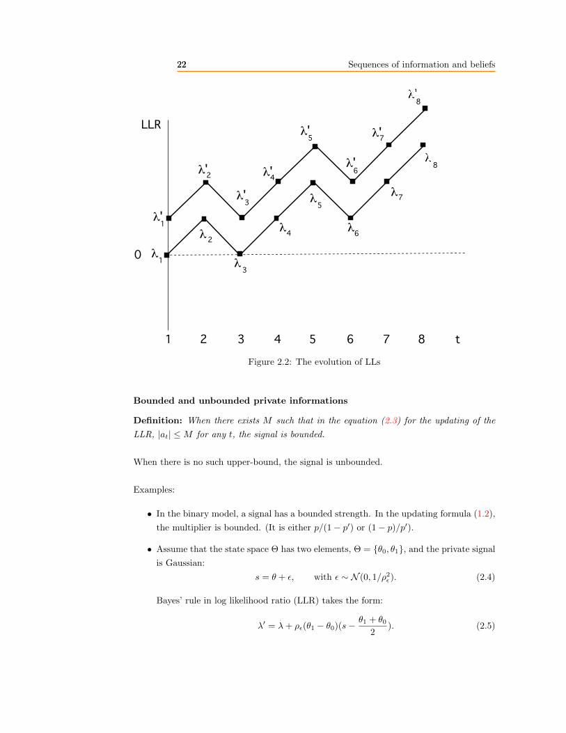
signals. The evolution of their LLRs is illustrated in Figure 2.2.
Note that upwards and downwards moves have the same magnitude. The LLR is obviously
not bounded. In the figure a LLR of 0 means equal probabilities for the two states. If the
LLR is negative, the state 0 is more likely.
We can generalize this to a model with a continuum of agents, of total mass that can
be taken equal to 1, each characterized by a prior belief. The distribution of prior beliefs
(measured in LLR) is characterized by a density function with support **, which is assumed
here to be a bounded interval of real numbers. When new information is received, the
evolution of the beliefs of the population is represented by (random) translations of the
support. For each of these supports, the density of the beliefs is the same as in the prior
distribution.
22 Sequences of information and beliefs22
t
0
1 2 3 4 5 6 7 8
λ1
λ 2
λ3
λ4
λ5
λ6
λ7
8
λ'1
λ'2λ'
3
λ'4
λ'5
λ'6
λ'7
8
LLR
Figure 2.2: The evolution of LLs
Bounded and unbounded private informations
Definition: When there exists M such that in the equation (2.3) for the updating of the
LLR, |at| ≤M for any t, the signal is bounded.
When there is no such upper-bound, the signal is unbounded.
Examples:
• In the binary model, a signal has a bounded strength. In the updating formula (1.2),
the multiplier is bounded. (It is either p/(1− p′) or (1− p)/p′).
• Assume that the state space Θ has two elements, Θ = θ0, θ1, and the private signal
is Gaussian:
s = θ + ε, with ε ∼ N (0, 1/ρ2ε). (2.4)
Bayes’ rule in log likelihood ratio (LLR) takes the form:
λ′ = λ+ ρε(θ1 − θ0)(s− θ1 + θ02
). (2.5)
23 Sequences of information and beliefs23
Since s is unbounded, the private signal has an unbounded impact on the subjective
probability of a state. There are values of s such that the likelihood ratio after
receiving s is arbitrarily large.
2.2 Martingales
Bayesian learning satisfies a strong property on the revision of the distribution of the states
of nature. Suppose that before receiving a signal s, our expected value of a real numberBayesian learning
satisfies the martingale
property: changes
of beliefs are
not predictable.
θ is E[θ]. This expectation will be revised after the reception of s. Question: given the
information that we have before receiving s, what is the expected value of the revision?
Answer: zero. If the answer were not zero, we would incorporate it in the expectation of
θ ex ante. This property is the martingale property. It is a central property of rational
(Bayesian) learning. The martingale property separates rational from non rational learning.
The martingale property with learning from a binary signal
Assume that there are two signal values, s =∈ 0, 1. Let P (θ) be the probability that θ
is equal to some value (or is in some set). P and P ′ denote prior (before the signal s) and
posterior probabilities.
E[P ′(θ)] = P (s = 1)P ′(θ|s = 1) + P (s = 0)P ′(θ|s = 0),
= P (s = 1)P (θ ∩ s = 1)
P (s = 1)+ P (s = 0)
P (θ ∩ s = 0)
P (s = 0),
= P (θ ∩ s = 1) + P (θ ∩ s = 0),
= P (θ ∩ (s = 1 ∪ s = 0)) = P (θ).
An equivalent result is
E[P ′(θ)− P (θ)] = 0.
Note that P (θ) is not a random variable: it is the probability of θ before the signal is
received. Before that reception, the expected value of the change of P (θ) (caused by the
observation of the signal), is equal to 0! P (θ) is a martingale. If there are two states
θ ∈ 0, 1, then E[θ] = P (θ = 1) and E[θ] satisfies the martingale property.
The martingale property holds in general for any form of signal and if θ takes arbitrary
values because it rests on the the property of conditional probabilities. Assume for example
that θ has a density g(θ), and that s has a density φ(s|θ) conditional on θ. Let ψ(θ|s)be the density of θ conditional on s. By Bayes’ rule, ψ(θ|s) = φ(s|θ)g(θ)/φ(s), with
φ(s) =∫φ(s|θ)g(θ)dθ. Using
∫φ(s|θ)ds = 1 for any θ,
24 Sequences of information and beliefs24
E[E[θ|s]
]=
∫ (∫θψ(θ|s)dθ
)φ(s)ds =
∫ ∫φ(s|θ)θg(θ)dsdθ =
∫θg(θ)dθ = E[θ].
The similarity of this property with that of an efficient financial market is not fortuitous:
in a financial market, updating is rational and it is rationally anticipated. Economists have
often used martingales without knowing it.
A little formalism is helpful at this point. Assume that information comes as a sequence
of signals st, one signal per period. Assume further that these signals have a distribution
which depends on θ. They may or may not be independent, conditional on θ, and their
distribution is known. Define the history in period t as ht = (s1, . . . , st). The martingale
property is defined for a sequence of real random variables as follows.1
DEFINITION 2.1. The sequence of random variables Yt is a martingale with respect to
the history ht = (s1, . . . , st−1) if and only if
Yt = E[Yt+1|ht].
Expanding on the example with a binary signal, denote µt = E[θ|ht]. Because the history
ht is random, µt is a sequence of random variables. The proof of the next result is the
same as for the simple example
PROPOSITION 2.1. Let µt = E[θ|ht] with ht = (s1, . . . , st−1). It satisfies the martin-
gale property: µt = E[µt+1|ht].
Let A be a set of values for θ, A ⊂ Θ, and consider the indicator function IA for the set Awhich is the random variable given by
IA(θ) =
1 if θ ∈ A,0 if θ /∈ A.
Using P (θ ∈ A) = E[IA] and applying the previous proposition to the random variable IAgives the next result.
PROPOSITION 2.2. The probability assessment of an event by a Bayesian agent is a
martingale: for an arbitrary set A ⊂ Θ, let µt = P (θ ∈ A|ht) where ht is the history of
informations before period t; then µt = E[µt+1|ht].
The likelihood ratio between two states θ1 and θ0 cannot be a martingale given the infor-
mation of an agent. However, if the state is assumed to take a particular value, then the
1A useful reference is Grimmet and Stirzaker (1992).
25 Sequences of information and beliefs25
likelihood ratio may be a martingale. Proving it is a good exercise.
PROPOSITION 2.3. Conditional on θ = θ0, the likelihood ratio
P (θ = θ1|ht)P (θ = θ0|ht)
is a martingale.
2.3 Convergence of beliefs
Probabilities will be equivalent to “beliefs”. When more information comes in, does a belief
(the probability estimate of a particular state) converge to some value. (We postpone the
question whether it converges to the truth). We first need a definition of convergence. In
this book, any convergence of a random variable (for example, a belief) is a convergence
in probabiity2:
DEFINITION 2.2. Let X1, X2, . . . , Xn, . . . be random variables on some probability space
(Ω,F , P ). Xn tends to a limit X in probability if
• for any given ε > 0, P (|Xn −X| ≥ ε)→ 0 as n→∞.
Note that the limit X is a random variable. For example, Xt may be a belief at history
ht. The sequence of beliefs converges but we don’t know to which value it will converge.
A great property of any rational learning process is that beliefs converge. This convergenceBayesian beliefs
converge because
of the Martingale
Convergence Theorem.
occurs because the sequence of beliefs is a martingale that is bounded (between 0 and 1
by definition of a probability) and the martingale convergence theorem (MCT) states that
any bounded martingale converges.
The convergence of a bounded martingale, in a sense which will be made explicit, is a
great result which is intuitive. The essence of a martingale is that its changes cannot be
predicted, like the walk of a drunkard in a straight alley. The sides of the alley are the
bounds of the martingale. If the changes of direction of the drunkard cannot be predicted,
the only possibility is that these changes gradually taper off. For example, the drunkard
cannot bounce against the side of the alley: once he hits the side, the direction of his next
move is predictable.
2There are other criteria of convergence, for example the convergence almost sure (on a set of measureone in Ω, or convergences of the expected value of |Xn|r, r ≥ 1), but these are not useful at this stage forthe analysis of the convergence of beliefs in a learning process. At this stage, there is no study of sociallearning with an example of convergence in probability and no convergence almost surely.
26 Sequences of information and beliefs26
THEOREM 2.1. (Martingale Convergence Theorem)3
If Xt is a martingale with |X| < M <∞ for some M and all t, then there exists a random
variable X such that Xt converges to X.
Most of the social learning in this book will be about probability assessments that the state
of nature belongs to some set A ⊂ Θ. We have seen that probability assessments satisfy
the martingale property. They are obviously bounded by 1. Therefore they converge to
some value.
PROPOSITION 2.5. Let A be a subset of Θ and µt be the probability assessment µt =
P (θ ∈ A|ht), where ht is a sequence of random variables in previous periods. Then there
exists a random variable µ∗ such that µt → µ∗.
Proof (hint): (“buy low, sell high”)
There are various proofs of the MCT. Recall that the martingale property is the same
as the efficient market equation. If a market is efficient, there is not strategy that has a
positive expected gain. One proof of the MCT rests on the fact that the strategy “buy low,
sell high” cannot generate a positive expected profit. Economists should have discovered
the MCT.
We want to show that a belief, the probability of a state, or of an event, converges. Call
that belief in round t, pt. The stock is traded for T periods and new information is coming
between periods. The truth is known in round T + 1. The stock pays 1 if the event takes
place and 0 otherwise. The sequence of prices pt is a martingale.
Take two numbers b and a with 0 < b < a < 1. The difference a − b may be small, but
this is not important right now. The trading strategy is to buy one unit of the stock if the
price is smaller than b, hold the stock until the price is higher than b, and sell the stock as
soon as the price is higher than a. A new stock is bought when the price goes below b. In
the strategy “buy low and sell high”. “Low” and “high” are defined by the two values b
and a.
If in period T , you hold the stock, you sell it at whatever the price in that period, pT . The
strategy is illustrated by Figure 2.3.
Define by NT the number of times you buy a stock until round T , that is the number of
upwards crossings of the band (b, a) in the trajectory of the price, pt. The maximum loss
3Recall that we use only the convergence in probability. The theorem shows, under weaker conditions,the stronger property that the martingale converges almost everywhere.
27 Sequences of information and beliefs27
Τ0
Μ
p
Buy
Sell
Hold
Buy
Sell
Buy
Sell
1 2 Round
Hold
The agent holds one unit of the asset on the red segments.
Figure 2.3: A strategy of “buy low, sell high”
is b (if he has a stock that he sells in the last period). The gain is NT (a− b). Since b < 1,
the net profit is not smaller than
V = NT (a− b)− 1.
Because of the martingale property, the expected gain from the trading strategy cannot be
positive. Hence, for any T ,
E[NT ] ≤ 1
(a− b) .
The expectation of the number of upward crossing is bounded. From this, one can show
that the probability of an upward crossing after period t tends to zero if t tends to infinity.
One can then divide the interval [0, 1] in n intervals, each of with 1/n and iterate the
previous argument for the finite number n. That means that for any ε, the stochastic
process stays within one of these bands except with probability ε. Since the number n can
be take as large as one wants, that proves the convergence in probability.4
A heuristic remark on another proof of the Martingale Convergence Theorem
The main intuition of the proof is important for our understanding of Bayesian learning. It
is a formalization6 of the metaphor of the drunkard. In words, the definition of a martingale
4From these intuitive hints, the reader can construct a formal proof. For verification, see Williams(1991).
6The proof is given in Grimmet and Stirzaker (1992). The different notions of convergence of a random
28 Sequences of information and beliefs28
states that agents do not anticipate systematic errors. This implies that the updating
difference µt+1 − µt is uncorrelated with µt. The same property holds for more distant
periods: conditional on the information in period t, the random variables µt+k+1 − µt+kare uncorrelated for k ≥ 0.
Since µt+n − µt =
n∑
k=1
µt+k − µt+k−1,
conditional on ht, V ar(µt+n) =
n∑
k=1
V ar(µt+k − µt+k−1).
Since E[µ2t+n] is bounded, V ar(µt+n) is bounded: there exists A such that
for any n,
n∑
k=1
V ar(µt+k − µt+k−1) ≤ A.
Since the sum is bounded, truncated sums after date T must converge to zero as T →∞:
for any ε > 0, there exists T such that for all n > T ,
V ar(µT+n − µT ) =
n∑
k=1
V ar(µT+k − µT+k−1) < ε.
The amplitudes of all the variations of µt beyond any period T become vanishingly small
as t→ 0. Therefore µt converges7 to some value µ∞. The limit value is in general random
and depends on the history.
Rational (Bayesian) beliefs cannot cycle forever
Another way to look at the convergence of rational beliefs is to ask why they cannot have
random cycles. If such cycles take place, there are random peaks and troughs, since the
beliefs are between 0 and 1. But then how can the belief evolve when, say, it is close to 1.
There is not much “room” to move up. Hence there cannot be much room to move down.
If the belief could move down by a large amount, then, since it cannot move up by much,
it should be have been adjusted right now. Of course, all this is in a probabilistic sense.
The belief may move down by a large amount, but the larger the jump down, the smaller
its probability. From this, we see that if the belief is close to 1, or to 0, it does not move
up or down very much between periods.
variable are recalled in the Appendix.
7The convergence of µt is similar to the Cauchy property in a compact set for a sequence xt: ifSupk(|xt+k − xt|)→ 0 when t→∞, then there is x∗ such that xt → x∗. The main task of the proof is to
analyze carefully the convergence of µt.
29 Sequences of information and beliefs29
One could also comment that if a belief, which has been generated by history is close to
1 , that means that history has provided convincing information that the event is highly
probable. Any new information is rationally combined with history but the “weight” of
this “convincing” history is such that new information can generate only a small change
of belief.
This deep property distinguishes rational Bayesian learning from other forms of learning.Rational beliefs
converge while
non rational beliefs
may not.
Many adaptative (mechanical) rules of learning with fixed weights from past signals are not
Bayesian and do not lead to convergence. In Kirman (1993), agents follow a mechanical
rule which can be compared to ants searching for sources of food, and their beliefs fluctuate
randomly and endlessly.
The evolution of confidence
When there are two states, the probability distribution is characterized by the probability
µ of the good state. This value determines an index of confidence: if the two states are 0
and 1, the variance of the distribution is µ(1− µ). Suppose that µ is near 1 and that new
information arrives which reduces the value of µ. This information increases the variance
of the estimate, i.e., it reduces the confidence of the estimate.
30 Sequences of information and beliefs30
EXERCISE 2.1. (Non independent signals)
Construct an example with non independent signals where the history at time t cannot
be summarized by the belief at time t.
31 Sequences of information and beliefs31
BIBLIOGRAPHY
Williams, David (1991-2004). Probability with Martingales, Cambridge University Press.
Grimmett, Geoffrey an David Stirzaker (1982-2001). Probability and random Processes,
Oxford University Press.
Park, Andreas and Hamid Sabourian (2011). “Herding and contrarian behavior in financial
markets,” Econometrica, 79, 973-1026.
32 Sequences of information and beliefs32
Chapter 3
Social learning
Why learn from others’ actions? Because these actions reflect something about their in-
formation. Why don’t we exchange information directly using words? People may not be
able to express their information well. They may not speak the same language. They may
even try to deceive us. What are we trying to find? A good restaurant, a good movie,
a tip on the stock market, whether to delay an investment or not,... Other people know
something about it, and their knowledge affects their behavior which, we can trust, must
be self-serving. By looking at their behavior, we will infer something about what they
know. This chain of arguments will be introduced here and developed in other chapters.
We will see how the transmission of information may or may not be efficient and may lead
to herd behavior, to sudden changes of widely believed opinions, etc...
For actions to speak and to speak well, they must have a sufficient vocabulary and be
intelligible. In the first model of this chapter, individuals are able to fine tune their
action in a sufficiently rich set and their decision process is perfectly known. In such
a setting, actions reflect perfectly the information of each acting individual. This case is a
benchmark in which social learning is equivalent to the direct observation of others’ private
information. Social learning is efficient in the sense that private actions convey perfectly
private informations.
Actions can reveal perfectly private informations only if the individuals’ decision processes
are known. But surely private decisions depend on private informations and on personal
parameters which are not observable. When private decisions depend on unobservable
idiosyncracies, or equivalently when their observation by others is garbled by some noise,
the process of social learning can be much slower than in the efficient case (Vives, 1993).
33
34 Social learning34
3.1 A canonical model of social learning
3.1.1 Structure
The purpose of a canonical model is to present a structure which is sufficiently simple and
flexible to be a tool of analysis for a number of issues. Many models of rational social
learning are built with the following three blocks:
1. The information endowments: The state of nature is what the information is about.
It is denoted by θ and is randomly chosen by nature before the learning process in a
set Θ that can be finite or in a continuum. The probability distribution of nature is
the prior distribution and is known to all agents.
2. The private information of an agent i, i = 1, . . . , N , where N can be infinite, is what
provides a value to others when they observe his action. That private information is
modeled here by a random signal si. That signal has a probability distribution that
is known by others in most cases (to make some inference possible), but by definition
of private, the realization of the signal si cannot be observed by others. The signal
provide some information on the state θ because its distribution depends on the true
value of the state of nature θ. Any agent updates the prior on θ with the signal si
to form a private distribution of probability of θ.
3. The action xi of agent i is taken in round i, (i ≥ 1) and belongs to a set Ξ. (Without
loss of generality, Ξ is the same set for all agents. The action will be the “message”.
We can assume here that this action is such that
x∗i = Ei[θ], (3.1)
where Ei is the expectation of agent i when the action is taken.
One can explain the decision rule in (3.1) by the optimization of the agent.
For example, it is the decision rule if the agent maximizes the expected value
of the payoff function −(x − θ)2 or the function θx − x2/2, which both have
a simple intuitive interpretation. However, this “structural foundation” of the
behavioral rule is not required here for the analysis of the social learning. Note
that for these two functions, the optimal payoff is equal to minus the variance
of θ (up to a constant). That may be convenient in evaluating the benefit of
information.
What is essential at this stage, is that agents other than i know that (3.1) is the
decision rule. We will deal later with the important case of an imperfect or imperfectly
known decision rule. One can also have other payoff functions but they may lead to
a more complex inference problem without additional insight.
35 Social learning35
Since agents “speak” through their actions, the definition of the action set Ξ is critical.
A language with many words may convey more possibilities for communication than a
language with few words. Individuals will learn more from each other about a parameter
θ when the actions are in an interval of real numbers than when the actions are restricted
to be either zero or one.
3.1.2 The process
In this chapter and the next, agents are ordered in an exogenous sequence. Agent t, t ≥ 1,
chooses his action in period t. We define the history of the economy in period t as the
sequence
ht = x1, . . . , xt−1, with h0 = ∅.Agent t knows the history of past actions ht before making a decision.
To summarize, at the beginning of period t (before agent t makes a decision), the knowledge
which is common to all agents is defined by
• the distribution of θ at the beginning of time,
• the distributions of private signals and the payoff functions of all agents,
• the history ht of previous actions.
We will assume that agents cannot observe the payoff of the actions of others. Whether
this assumption is justified or not depends on the context. It is relevant for investment
over the business cycle: given the lags between investment expenditures and their returns,
one can assume that investment decisions carry the sole information. Later in the book,
we will analyze other mechanisms of social learning. For the sake of clarity, it is best to
focus on each one of them separately.
Agent t combines the public belief on θ with his private information (the signal st) to form
his belief which has a c.d.f. F (θ|ht, st). He then chooses the action xt to maximize his
payoff E[u(θ, xt)], conditional on his belief.
All remaining agents know the payoff function of agent t (but not the realization of the
payoff), and the decision model of agent t. They use the observation of xt as a signal on
the information of agent t, i.e., his private signal st. The action of an agent is a message
on his information. The social learning depends critically on how this message conveys
information on the private belief. The other agents update the public belief on θ once
the observation xt is added to the history ht: ht+1 = (ht, xt). The distribution F (θ|ht) is
updated to F (θ|ht+1).
36 Social learning36
3.2 The Gaussian model
Social learning is efficient when an individual’s action reveals completely his private infor-
mation. This occurs when the action set which defines the vocabulary of social learning is
sufficiently large. We begin with the Gaussian model (Section ??) that provides a simple
and precise case for discussion.
The prior distribution on θ is normal, N (m1, 1/ρ1), with mean m1 and precision ρ1. Since
we focus on the social learning of a given state of nature, the value of θ does not change
once it is set.
There is a countable number of individuals, indexed by i ≥ 1, and each individual i has
one private signal si such that
si = θ + εi, with εi ∼ N (0, 1/ρε).
Individual t chooses his action xt ∈ R once and for all in period t: the order of the
individual actions is set exogenously.
The public information at the beginning of period t is made of the initial distribution
N (θ, 1/ρθ) and of the history of previous actions ht = (x1, . . . , xt−1).
Suppose that the public belief on θ in period t is given by the normal distributionN (µt, 1/ρt).
This assumption is obviously true for t = 1. By induction, we now show that it is true in
every period.
(i) The belief of agent t
The belief is obtained from the Bayesian updating of the public belief N (µt, 1/ρt) with
the private information st = θ + εt. Using the standard Bayesian formulae with Gaussian
distributions, the belief of agent t is N (µt, 1/ρt) with
µt = (1− αt)µt + αtst, with αt =
ρερε + ρt
,
ρt = ρt + ρε.
(3.3)
(ii) The private decision
From the specification of µt in (3.3),
xt = (1− αt)µt + αtst. (3.4)
37 Social learning37
(iii) Social learning
The decision rule of agent t and the variables αt, µt are known to all agents. From equationSocial learning
is efficient when
actions reveal
perfectly private
informations.
(3.4), the observation of the action xt reveals perfectly the private signal st. This is a key
property. The public information at the end of period t is identical to the information of
agent t: µt+1 = µt, and ρt+1 = ρt. Hence,
µt+1 = (1− αt)µt + αtst, with αt =
ρερε + ρt
,
ρt+1 = ρt + ρε.
(3.5)
In period t+ 1, the belief is still normally distributed N (µt+1, 1/ρt+1) and the process can
be iterated as long as there is an agent remaining in the game. The history of actions
ht = (x1, . . . , xt−1) is informationally equivalent to the sequence of signals (s1, . . . , st−1).
Convergence
The precision of the public belief increases linearly with time:
ρt = ρθ + (t− 1)ρε, (3.6)
and the variance of the estimate on θ is σ2t = 1/(ρθ + tρε), which converges to zero like
1/t. This is the rate of the efficient convergence.
The weight of history and imitation
Agent t chooses an action which is a weighted average of the public information µt from
history and his private signal st (equation (3.4)). The expression of the weight of history,
1 − αt, increases and tends to 1 when t increases to infinity. The weight of the privateImitation increases
with the weight
of history, but
does not slow down
social learning
if actions reveal
private informations.
signal tends to zero. Hence, agents tend to “imitate” each other more as time goes on. This
is a very simple, natural and general property: a longer history carries more information.
Although the differences between individuals’ actions become vanishingly small as time
goes on, the social learning is not affected because these actions are perfectly observable:
no matter how small these variations, observers have a magnifying glass which enables
them to see the differences perfectly. In the next section, this assumption will be removed.
An observer will not“see” well the small variations. This imperfection will slow down
significantly the social learning.
3.3 Observation noise
In the previous section, an agent’s action conveyed perfectly his private information. An
individual’s action can reflect the slightest nuances of his information because: (i) it is
38 Social learning38
chosen in a sufficiently rich menu; (ii) it is perfectly observable; (iii) the decision model of
each agent is perfectly known to others.
The extraction of information from an individual’s action relies critically on the assumption
that the decision model is perfectly known, an assumption which is obviously very strong.
In general, individuals’ actions depend on a common parameter but also on private char-
acteristics. It is the essence of these private characteristics that they cannot be observed
perfectly (exactly as the private information is not observed by others). To simplify, assume
that the observation of the action of agent i is given by
xi = Ei[θ] + ηi, with ηi ∼ N (0, 1/ρη). (3.7)
The noise ηi is independent of other random variables and it can arise either because
there is an observation noise or because the payoff function of the agent is subject to an
idiosyncratic variable.1
Since the private parameter ηi is not observable, the action of agent i conveys a noisy
signal on his information Ei[θ]. Imperfect information on an agent’s private characteristics
is operationally equivalent to a noise on the observation of the actions of an agent whose
characteristics are perfectly known.
The model of the previous section is now extended to incorporate an observation noise,
along the idea of Vives (1993)2. We begin with a direct extension of the model where there
is one action per agent in each period. The model with many agents is relevant in the case
of a market and will be presented in Section 3.2.
An intuitive description of the critical mechanism
Period t brings to the public information the observation
xt = (1− αt)µt + αtst + ηt, with αt =ρε
ρt + ρε. (3.8)
The observation of xt does not reveal perfectly the private signal st because of a noise
ηt ∼ N (0, σ2η). This simple equation is sufficient to outline the critical argument. As
time goes on, the learning process increases the precision of the public belief on θ, ρt,
which tends to infinity. Rational agents imitate more and reduce the weight αt which they
put on their private signal as they get more information through history. Hence, they
reduce the multiplier of st on their action. As t → ∞, the impact of the private signal
st on xt becomes vanishingly small. The variance of the noise ηt remains constant over
1For example if the payoff is −(xi − θ − ηi)2.2Vives assumes directly an observation noise and a continuum of agents. His work is discussed below.
39 Social learning39
time, however. Asymptotically, the impact of the private information on the level of action
becomes vanishingly small relative to that of the unobservable idiosyncracy. This effect
reduces the information content of each observation and slows down the process of social
learning.
Imitation increases
with the weight
of history and
reduces the signal
to noise ratio of
private actions.The impact of the noise cannot prevent the convergence of the precision ρt to infinity.
By contradiction, suppose that ρt is bounded. Then αt does not converge to zero and
the precision ρt increases linearly, asymptotically (contradicting the boundedness of the
precision). The analysis now confirms the intuition and measures accurately the impact of
the noise on the rate of convergence of learning.
The evolution of beliefs
Since the private signal is st = θ + εt with εt ∼ N (0, σ2ε ), equation (3.8) can be rewritten
xt = (1− αt)µt + αtθ + αtεt + ηt.︸ ︷︷ ︸noise term
(3.9)
The observation of the action xt provides a signal on θ, αtθ, with a noise αtεt + ηt. We
will encounter in this book many similar expressions of noisy signals on θ. We use a
simple procedure to simplify the learning rule (3.9): the signal is normalized by aA standard normalization
will be used for
most Gaussian signals.linear transformation such that the right-hand side is the sum of θ (the parameter to be
estimated), and a noise:
xt − (1− αt)µtαt
= zt = θ + εt +ηtαt. (3.10)
The variable xt is informationally equivalent to the variable zt. We will use similar equiva-
lences for most Gaussian signals. The learning rules for the public belief follow immediately
from the standard formulae with Gaussian signals (3.3). Using (3.8), the distribution of θ
at the end of period t is N (µt+1, 1/ρ2t+1) with
µt+1 = (1− βt)µt + βt
(xt − (1− αt)µtαt
), with
βt =σ2t
σ2t + σ2
ε + σ2η/α
2t
,
ρt+1 = ρt + 1
σ2ε + σ2
η/α2t
= ρt +1
σ2ε + σ2
η(1 + ρtσ2ε )2
.
(3.11)
Convergence
When there is no observation noise, the precision of the public belief ρt increases by a
constant value ρε in each period, and it is a linear function of the number of observations
(equation (3.6)). When there is an observation noise, equation (3.11) shows that as ρt →∞,
40 Social learning40
the increments of the precision, ρt+1 − ρt, becomes smaller and smaller and tend to zero.
The precision converges to infinity at a rate slower than a linear rate. The convergence of
the variance σ2t to 0 takes place at a rate slower than 1/t.
The slowing down of the convergence when actions are observed through a noise has been
formally analyzed by Vives (1993). In a remarkable result, he showed that the precision of
the public information, ρt increases only like the cubic root of the number of observations,
At1/3. The value of the constant A depends on the observation noise, but the rate 1/3 is
independent of that variance. Recall that with no noise, the precision increases linearly
with t.
When the number of observations is large, 1000 additional observations with noise generate
the same increase of precision as 10 observations when there is no observation noise.
The result of Vives shows that the standard model of social learning where agents observe
perfectly others’ actions and know their decision process is not robust. When observations
are subject to a noise, the process of social learning is slowed down, possibly drastically,
because of the weight of history. That weight reduces the signal to noise ratio of individual
actions. The mechanism by which the weight of history reduces social learning will be
shown to be robust and will be one of the important themes in the book.
3.3.1 Large number of agents
The previous model is modified to allow for a continuum of agents. Each agent is indexed
by i ∈ [0, 1] (with a uniform distribution) and receives one private signal once at the
beginning of the first period3, si = θ + εi, with εi ∼ N (0, σ2ε ). Each agent takes an action
xt(i) in each period4 t to maximize the expected quadratic payoff in (??). At the end of
period t, agents observe the aggregate action Yt which is the sum of the individuals’ actions
and of an aggregate noise ηt:
Yt = Xt + ηt, with Xt =
∫xt(i)di, and ηt ∼ N (0, 1/ρη).
At the beginning of any period t, the public belief on θ is N (µt, 1/ρt), and an agent with
3If agents were to receive more than one signal, the precision of their private information would increase
over time.
4One could also assume that there is a new set of agents in each period and that these agents act onlyonce.
41 Social learning41
By the law of large numbers5,∫εidi = 0. Therefore, αt
∫sidi = αtθ. The level of
endogenous aggregate activity is
Xt = (1− αt)µt + αtθ,
and the observed aggregate action is
Yt = (1− αt)µt + αtθ + ηt. (3.12)
Using the normalization introduced in Section ??, this signal is informationally equivalent
toYt − (1− αt)µt
αt= θ +
ηtαt
= θ +(
1 +ρtρε
)ηt. (3.13)
This equation is similar to (3.10) in the model with one agent per period. (The variances
of the noise terms in the two equations are asymptotically equivalent). Proposition ??
applies. The asymptotic evolutions of the public beliefs are the same in the two models.
Note that the observation noise has to be an aggregate noise. If the noises affected actions
at the individual level, for example through individuals’ characteristics, they would be
“averaged out” by aggregation, and the law of large numbers would reveal perfectly the
state of nature. An aggregate noise is a very plausible assumption in the gathering of
aggregate data.
3.3.2 Application: a market equilibrium
This setting is the original model of Vives (1993). A good is supplied by a continuum of
identical firms indexed by i which has a uniform density on [0, 1]. Firm i supplies xi and
the total supply is X =∫xidi. The demand for the good is linear:
p = a+ η − bX. (3.14)
Each firm (agent) i is a price taker and has a profit function
ui = (p− θ)xi −c
2x2i ,
where the last term is a cost of production and θ is an unknown parameter. Vives views
this parameter as a pollution cost which is assessed and charged after the end of the game.
As in the canonical model, nature’s distribution on θ is N (µ, 1/ρθ) and each agent i has a
private signal si = θ + εi with εi ∼ N (0, 1/ρε). The expected value of θ for firm i is
Ei[θ] = (1− α)µ+ α(θ + εi), with α =ρε
ρθ + ρε. (3.15)
5A continuum of agents of mass one with independent signals is the limit case of n agents each of mass1/n where n→∞. The variance of each individual action is proportional to 1/n2 and the variance of theaggregate decision is proportional to 1/n which is asymptotically equal to zero.
42 Social learning42
The optimal decision of each firm is such that the marginal profit is equal to the marginal
cost:
p− Ei[θ] = cxi.
Integrating this equation over all firms and using the market equilibrium condition (3.14)
gives
p−∫Ei[θ]di = cX =
c
b(a+ η − p),
which, using (3.15), is equivalent to
(b+ c)p− ac− (1− α)µ = αθ + cη.
Dividing both sides of this equation to normalize the signal, the observation of the market
price is equivalent to the observation of the signal
Z = θ + cη
α, where α =
ρερθ + ρε
.
The model is isomorphic to the canonical model of the previous section.
3.4 Extensions
Endogenous private information
See exercise 3.1.
Policy against mimetism
A selfish agent who maximizes his own welfare ignores that his action generates informa-
tional benefits to others. If the action is observed without noise, it conveys all the private
information without any loss. But if there is an observation noise, the information con-
veyed by the action is reduced when the response of the action is smaller. When time goes
on, the amplitude of the noise is constant and the agent rationally reduces the multiplier
of his signal on his action. Hence, the action of the agent conveys less information about
his signal when t increases. A social planner may require that agents overstate the impact
of their private signal on their action in order to be “heard” over the observation noise.
Vives (1997) assumes that the social welfare function is the sum of the discounted payoffs
of the agents
W =∑
t≥0βt(−Et[(xt − θ)2]
),
where xt is the action of agent t. All agents observe the action plus a noise, yt = xt + εt.
The function W is interpreted as a loss function as long as θ is not revealed by a random
exogenous process. In any period t, conditional on no previous revelation, θ is revealed
43 Social learning43
perfectly with probability 1 − π ≥ 0. Assuming a discount factor δ < 1, the value of β is
β = πδ. If the value of θ is revealed, there is no more loss.
As we have seen in (3.3) and (3.4), a selfish agent with signal st has a decision rule of the
form
xt − µt = (1 + γ)ρε
ρt + ρε(st − µt), (3.16)
with γ = 0. Vives assumes that a social planner can enforce an arbitrary value for γ.
When γ > 0, the action to noise ratio is higher and the observers of the action receive
more information.
Assume that a selfish agent is constrained to the decision rule (3.16) and optimizes over γ:
he chooses γ = 0. By the envelope theorem, a small first order deviation of the agent from
his optimal value γ = 0 has a second order effect on his welfare. We now show that it has
a first order effect on the welfare of any other individual who make a decision. The action
of the agent is informationally equivalent to the message
y = (1 + γ)αs+ ε, with α =ρε
ρt + ρε.
The precision of that message is ρy = (1 + γ)2α2ρε.
Another individual’s welfare is minus the variance after the observation of y. The obser-
vation of y adds an amount ρy to the precision of his belief. If γ increases from an initial
value of 0, the variation of ρy is of the order of 2γα2ρε, i.e., of the first order with respect to
γ. Since the variance is the inverse of the precision, the impact on the variance of others is
also of the first order and dwarfs the second order impact on the agent. There is a positive
value of γ which induces a higher social welfare level.
44 Social learning44
EXERCISES
EXERCISE 3.1. (Endogenous private information)
In the standard Gaussian model of social learning, each agent has to pay of fixed cost c
to get a signal with precision ρ which is
s = θ + ε, with ε ∼ N (0, 1/ρ).
The cost c is assumed to be small. Agent t makes a decision in period t (both on the signal
and on the action), and his action is assumed to be perfectly observable by others. The
payoff function of each agent is quadratic: U(x) = E[−(x− θ)2].
1. Show using words and no algebra, that there is a date T after which no agent buys
a private signal. What happens to information and actions after that date T?
2. Provide now a formal proof of the the previous statement. For this compute the
welfare gain that an agent gets by buying a signal.
3. Assume now that the cost of a signal with precision ρ is an increasing function,6 c(ρ).
Prove the following result:
• Suppose that c′(ρ) is continuous and c(0) = 0. If the marginal cost of precision
c′(ρ) is bounded away from 0, (for any ρ ≥ 0, c′(ρ) ≥ γ > 0), no agent purchases
a signal after some finite period T and social learning stops in that period.
4. Assume now that c(q) = qβ with β > 0. Analyze the rate of convergence of social
learning.
REFERENCES
Burguet, R. and X. Vives, (2000). “Social Learning and Costly Information Acquisition,”
Economic Theory, 15, 185-205, (first version 1995).
Jun, B. and X. Vives (1996). “Learning and Convergence to a Full-Information Equilibrium
are Not Equivalent,” Review of Economic Studies, 63, 653-674.
6Suppose for example that the signal is generated by a sample of n independent observations and thateach observation has a constant cost c0. Since the precision of the sample is a linear function of n, thecost of the signal is a step function. For the sake of exposition, we assume that ρ can be any real number.
45 Social learning45
Lee, In Ho (1992). “On the Convergence of Informational Cascades,” Journal of Economic
Theory, 61, 395-411.
Vives, X. (1993). “How Fast Do Rational Agents Learn?,” Review of Economic Studies,
60, 329-347.
Vives, X. (1996). “Social Learning and Rational Expectations,” European Economic Re-
view, 40, 589-601.
Vives, X. (1997). “Learning From Others: a Welfare Analysis,” Games and Economic
Behavior, 20, 177-200.
46 Social learning46
Chapter 4
Cascades and herds
A tale of two restaurants
Two restaurants face each other on the main street of a charming alsatian village. There is
no menu outside. It is 6pm. Both restaurants are empty. A tourist comes down the street,
looks at each of the restaurants and goes into one of them. After a while, another tourist
shows up, evaluates how many patrons are already inside by looking through the stained
glass windows—these are alsatian winstube—and chooses one of them. The scene repeats
itself with new tourists checking on the popularity of each restaurant before entering one
of them. After a while, all newcomers choose the same restaurant: they choose the more
popular one irrespective of their own information. This tale illustrates how rational people
may herd and choose one action because it is chosen by others. Among the many similar
stories, two are particularly enlightening.
High sales promote high sales
In 1995, management gurus Michael Reacy and Fred Wiersema secretly purchased 50,000
copies of their business strategy book The Discipline of Market Leaders from stores which
were monitored for the bestseller list of the New York Times1. The authors must have
been motivated by the following argument: people observe the sales, but not the payoffs of
the purchases (assuming they have few opportunities to meet other readers). Of course, if
the manipulation had been known it would have had no effect, but people rationally expect
that for any given book, the probability of manipulation is small, and that the high sales
must be driven by some informed buyers.
1See Bikhchandani, Hirshleifer and Welch (1998), and Business Week, August 7, 1995. Additionalexamples are given in Bikhchandani, Hirshleifer and Welch, (1992).
47
48 Cascades and herds48
The previous story illustrates one possible motivation for using the herding effect but it
is only indicative. For an actual measurement, we turn to Hanson and Putler (1996)
who conducted a nice experiment which combines the control of a laboratory with a “real
situation”. They manipulated a service provided by America Online (AOL) in the summer
of 1995. Customers of the service could download games from a bulletin board. The games
were free, but the download entailed some cost linked to the time spent in trying out the
game. Some games were downloaded more than others.
The service of AOL is summarized by the window available to subscribers which is re-
produced in Figure ??: column 1 shows the first date the product was available; column
2 the name of the product, which is informative; column 4 the most recent date the file
was downloaded. Column 3 is the most important and shows the number of customers
who have downloaded the file so far. It presents an index of the “popularity” of the prod-
uct. The main goal of the study is to investigate whether a high popularity increases the
demand ceteris paribus.
Figure 4.1: Applications for downloads
The impact of a treatment is measured by the increase in the number of downloads per day,
after the treatment, as a fraction of the average daily download (for the same product)
49 Cascades and herds49
before the treatment. The results are reported in Figure ??. All treatments have an
impact and the impact of the heavy treatment (100 percent) is particularly remarkable.
The experiment has an obvious implication for the general manipulation of demand through
advertisements.
Figure 4.2: Results
To ensure ceteris paribus, Hanson and Putler selected pairs of similar files which were
offered by AOL. Similarity was measured by characteristics and “popularity” at a specific
date. Once a pair was selected, one of the files was kept as the “control”, the other
was the “treatment”. The authors boosted the popularity index of the treatment file by
downloading it repeatedly. The popularity indexed was thus increased in a short session
by percentage increments of 25, 50 and 100. Customers of the service were not aware that
they were manipulated.
The essential issue and the framework of analysis
The previous examples share a common feature which is essential: individuals observe
the actions of others (and not their satisfaction), and the space of actions is discrete. The
actions are the words for the communication of information between agents. In the previous
50 Cascades and herds50
chapter, agents chose an action in a rich set (e.g., the set of real numbers), where even the
smallest differences between beliefs could be expressed. Here the finite number of actions
exerts a strong restriction on the vocabulary of social communication.
Bikchandani, Hirshleifer and Welch (1992), hereafter BHW, introduced the definition of
informational cascades in models of Bayesian learning.2 In a cascade, the public belief,
which is gathered from the history of observations, dominates the private information of
any individual: the action of any agent does not depend on his private information and all
agents are herding. Since actions do not convey information, nothing is learned and the
cascade goes on forever, possibly with an incorrect action. In the previous chapter we saw
how observation noise slows down the process of social communicatioin. Here, it eventually
comes to a complete stop.
A cascade generates a herd, but the concepts of cascade and herd are distinct. In aThere is an essential
difference between
a cascade and a
herd.
cascade, all agents ignore their information and take the same action. That behavior is
known by all. Hence any agent can predict the behavior of others, before they take action
and nothing is learned from the observation of others. In some way, the informational
cascade is an ex ante concept.
In a herd, all agents turn out to take the same action. The action of an agent cannot
be predicted before it is taken. Hence, something is learned from the observation of that
action. For example, after an “investment”, the belief in a “good state” is reinforced
because there was the possibility that the agent would have not invested. In a herd with
investment, the belief in the good state gradually increases. One should stress that here,
agents can never know that a herd takes place. In this sense, a herd is an post concept.
Of course, a informational cascade generates a herd, and in this case, agents do know that
they are in a herd. But the previous description hints at herds with no cascade. A cascade
implies a herd, but the reverse is not true. In fact, we will see that in a setting where
agents take discrete actions and no cascade occurs, a herd must eventually take place.
The simplest model of cascades is presented in Section 4.1. No formal arithmetics are
required for that section which presents the important properties. The general model is
analyzed in Section 4.2. The conditions for informational cascades are shown to be discrete
actions and bounded private beliefs. If private beliefs are unbounded, then there is always
the possibility that some agent with sufficiently strong and contrarian belief to diverge
2The expression “cascade” may be inappropriate for the description of a frozen behavior. Comparewith the description of a cascade in the prologue of Faust II. One should also point that the expression“cascade” was already used by Gabriel Tarde (1890), in the same sense as BHW. (See the bibliographicalnote).
51 Cascades and herds51
from “the crowd”. In this case, no cascade ever takes place. However, in this case, the
public belief converges to the truth. The public belief of the state tends to 1 or 0 and
the bar for the strength of a contrarian belief is higher and higher. As the probability
of a contrarian agent becomes smaller and smaller–a property that generates the ex post
herd–one learns less and less from the observation of others. Although no informational
cascade takes place, the social learning becomes vanishing small, asymptotically, which,
from a welfare point of view, is not very different from an informational cascade where
learning completely stops after finite time.
Section 4.4 presents a detailed analysis of herds and the convergence of beliefs3. Herds
always take place eventually, as a consequence of the Martingale Convergence Theorem.
There is in general some learning in a herd, but that learning is very slow. The conclusions
of the simple model of BHW are shown to be extraordinarily robust. They reinforce the
central message of the models of learning from others which is the self-defeating property
of social learning when individuals use rationally the public information.
4.1 The basic model of cascades
Students sometimes wonder how to build a model. Bikhchandani, Hirshleifer and WelshA textbook case
on how to build a
model(1992), hereafter BHW, provide an excellent lesson of methodology4: (i) a good story
simplifies the complex reality and keeps the main elements; (ii) this story is translated
into a set of assumptions about the structure of a model (information of agents, payoff
functions); (iii) the equilibrium behavior of rational agents is analyzed; (iv) the robustness
of the model is examined through extensions of the initial assumptions.
We begin here with the tale of two restaurants, or a similar story where agents have to
decide whether to make a fixed size investment. We construct a model with two states
(defining which restaurant is better), two signal values (which generate different beliefs),
and two possible actions (eating at one of two restaurants)5.
3For this section, I have greatly benefited from the insights of Lones Smith.
4Banerjee (1992) presented at the same time another paper on herding, but its structure is more
idiosyncratic and one cannot analyze the robustness of its properties.
5The example of the restaurants at the beginning of this chapter is found in Banerjee (1992). The model
in this section is constructed on this story. It is somewhat mistifying that Banerjee after introducing herdingthrough this example, develops an unrelated model which is somewhat idiosyncratic. A simplified version
is presented in Exercise 4.2.
52 Cascades and herds52
The 2 by 2 by 2 model
As in any model of Bayesian social learning, the structure has three blocks, the state of
nature, the private informations, the private decisions for action and the observation of
these actions.
1. The state of nature θ has two possible values, θ ∈ Θ = 0, 1, and is set randomly
once and for all at the beginning of the first period6 with a probability µ1 for the
state θ = 1. The value of θ could be the payoff of making a fixed size investment of 1.
It could also be defined as “restaurant A is better than B” (with θ = 0 representing
the opposite proposition).
2. N or a countable number of agents are indexed by the integer t. Each agent’s private
information takes the form of a SBS (symmetric binary signal) with precision q > 1/2:
P (st = θ | θ) = q. The signal represents the private information of an investor. It
could also represent the information of a travel book or a friend’s recommendation
about the quality of restaurant.
3. Agents take an action in an exogenous order as in the previous models of social
learning. The notation can be chosen such that agent t can make a decision in period
t and in period t only. An agent chooses his action x in the discrete set X = 0, 1.The action x = 1 may represent entering a restaurant, hiring an employee, or in
general making an investment of a fixed size. The yield of the action x depends on
the state of nature and is defined by
u(x, θ) =
0, if x = 0,
θ − c, if x = 1, with 0 < c < 1.
Since x = 0 or 1, another representation of the payoff is u(x, θ) = (θ − c)x. The
cost of the investment c is fixed.7 The yield of the investment is positive in the good
state and negative in the bad state. Under uncertainty, the payoff of the agent is the
expected value of u(x, θ) conditional on the information of the agent.
4. As in the previous models of social learning, the information of agent t is his private
signal and the history ht = (x1, . . . , xt−1) of the actions of the agents who precede
him in the exogenous sequence. The public belief at the beginning of period t is the
probability of the good state conditional on the history ht which is public information.
6The value of θ does not change because we want to analyze the changes in beliefs which are caused
only by endogenous behavior. Changes of θ can be analyzed in a separate study (see the bibliographicalnotes).
7In the tale of two restaurants, c could be taken as 1/2.
53 Cascades and herds53
It is denoted by µt:
µt = P (θ = 1|ht).
Without loss of generality, µ1 is the same as nature’s probability of choosing θ = 1.
Let us use the representation of the social learning in Log likelihood as in Figure 2.2. The
Log likelihood ratio between states 1 and 0 in the public information at the beginning of
period t is λt. We call optimists the agents with signal s = 1 and pessimists the other
ones. Agent t combines the public belief with his private signal to form his belief. Let λ+t
and λ−t the belief of an optimist or a pessimist in period t. We have seen (2.3) that
λ+t = λt + a, λ−t = λt − a, with a = Log(q/(1− q)),
and that the LLR “distance” between agents is constant in the process of social learning.
A geometric representation
Agent t takes action 1 if his belief (in state 1) is greater than c, which is equivalent to a
LLR greater than Log(c/(1 − c)). Let us denote γ = Log(c/(1 − c)). Note that in the
example of the two restaurants, c = 1/2 and γ = 0. The social learning is now represented
in Figure 4.1 where the LLR is measured along the vertical axis.
In each period, a segment represents the distribution of beliefs: the top of the segment
represents the belief of an optimist, the bottom the belief of a pessimist and the mid-point
the public belief. The segments evolve randomly over time according to the observations.
In the first period, the belief of an optimist, λ+1 , is above γ while the belief of a pessimist,
λ−1 , is below γ. The action is equal to the signal of the agent and thus reveals that signal.
In the figure, s1 = 0, and the first agent does not invest. His information is incorporated
in the public information: the public belief in the second period, λ2, is identical to the
belief of the first agent: λ2 = λ−1 . The sequence of the signal ndowments is indicated in
the figure. When there is social learning, the signal of agent t is integrated in the public
information of period t+ 1.
Consider now period 5 in the figure: agent 5 is an optimist, invests and eveals his signal
since he could have been a pessimist who does not invest. His information is incorporated
in the public belief of the next period and λ6 = λ+5 . The belief of a pessimist in period 6 is
now higher than the cost c (here, it is equal to the public belief λ5). In period 6, the belief
of an agent is higher than the cost of investment, whatever his signal. He invests, nothing
is learned and the public belief is the same in period 7: a cascade begins in period 6. The
54 Cascades and herds54
!
"
# $
# %
#
&
# '
#
(
# )
# &
* '
*
"
* $
* %
*
(
* )
*
"
(
'
+
+
"
,
--
-
" ( $ ) % & '
In each period, the middle of the vertical segment is the public belief, while the top and thebottom of the segment are the beliefs of an optimist (with a private signal s = 1) and of apessimist (with signal s = 0). The private signals are s1 = 0, s2 = 1, s3 = 0, s4 = 1, s5 = 1.(Ignore the horizontal line at 1).
Figure 4.3: Cascade representation
γ( )
λ
λ
λ
cascade takes place because all the beliefs are above the cut-off level c. This condition is
met here because the public belief λ6 is strictly higher than λ∗∗. Since λ6 is identical to
the belief of an optimist in period 5, the cascade occurs because the beliefs of all investing
agents are strictly higher than λ∗∗ in period 5. A cascade takes place because of the high
belief of the last agent who triggers the cascade.
Proposition 4.1 formalizes the previous discussion. It is expressed in beliefs µt = P (θ =
1|ht).
PROPOSITION 4.1. In any period t, given the public belief µt:
if µ∗ < µt ≤ µ∗∗, agent t invests if and only if his signal is good (st = 1);
if µt > µ∗∗, agent t invests independently of his signal;
if µt ≤ µ∗, agent t does not invest independently of his signal.
55 Cascades and herds55
4.2 Beyond the simple model
We keep the structure with two states θ ∈ 0, 1, two actions x ∈ 0, 1, with a payoff
(E[θ] − c)x, 0 < c < 1. The states 1 and 0 will be called “good” and “bad”. We extend
the previous model to admit any distribution of private beliefs that is generated by private
signals. Such a distribution is characterized by the c.d.f. F θ(µ) which depends on the state
θ. F θ(µ) denotes the c.d.f. of a distribution of the beliefs measured as the probability of θ1,
and F θ(λ) denotes the c.d.f. of a distribution of the LLR between θ1 and θ0. A graphical
representation of the distributions of beliefs in LLR is given in Figure (See also exercise
??).
λ0The distribution of private beliefs is represented by thecurves with θ = 1 and θ = 0 in the two states.
Figure 4.4: Distribution of beliefs (in LLR)
Note that the mass of probabilities is shifted upwards (downwards) when θ = 1 (θ = 0):
in the good state, more agents are optimistic. This can be observed if private signals are
symmetric binary with precision q and q is drawn from a distribution. The shape of the
distribution of beliefs in LLR is invariant to the news. We have seen in ** that any new
information has the same additive impact (positive or negative) on the LLR of any agent.
The news just translate the distribution.
In Figure 4.2, the distribution of beliefs, as in Figure 4.2, is be placed in the diagram of
Figure ?? that illustrates the process of social learning. In any period, the acting agent’s
belief is drawn from the distribution that is determined by the state. An example is
represented by the red arrows with LLR λ1, λ2 and λ3 in the first three rounds.
If the belief is above the cutoff level (0 in the figure), then the agent takes x = 1. Otherwise,
he takes x = 0. The probability that this belief in LLR is positive is greater in the good
state. It is proportional to the area in blue in the good state and in red in the other state.
Therefore, when other agents observe x = 1, they increase their belief in the good state.
By how much?
56 Cascades and herds56
λLLR
x = 1
x = 1
1
2
t = 1 t = 2 t = 3
t = 4
λ
λ
λ
1
2
3 x = 03
The distribution of private beliefs is represented by the curves with θ = 1and θ = 0 in the two states. In any period, the belief of the acting agentis taken randomly from the distribution that corresponds to the state.If his belief is above (below) the cut-off line (here 0), his takes x = 1(x = 0). See the discussion in the text.
Figure 4.5: Representation with a general bounded distribution of beliefs
Take the point of view of an outside observer. For him, x1 is just a binary signal on the
state. That signal is characterized by the probabilities x1 = 1 for each of the two states.
Here, the matrix of the probabilities takes the following form.
States of
Nature
Observations
xt = 1 xt = 0
θ = θ1 1− F θ1t (γ) F θ1t (γ)
θ = θ0 1− F θ0t (γ) F θ0t (γ)
For example, if θ = θ1, the probability that the acting agent has a LLR below γ is F θ11 (γ).
One can then fill the other elements of the matrix.
The update of the LLR after the observation of xt is, for an agent with LLR equal to λt
(any value), is determined as in (??) which is repeated here.
57 Cascades and herds57
λt+1 = λt + νt, with νt = Log(P (xt|θ1)
P (xt|θ0)
). (4.1)
As we have seen before, the updating term νt is independent of the belief λt. Therefore,
the distribution of beliefs is translated by a random term νt from period t to period t+ 1.
Agent t invests if and only if his probability of the good state is greater than his cost, i.e.
if his LLR, λ, is greater than γ = Log(c/(1 − c)). The probability that agent t invests
depends on the state and is equal to πt(θ) = 1− F θt (γ), with γ = Log( c
1− c).
Given the above matrix of the signal xt,
λt+1 = λt + νt, with νt =
Log(1− F θ1t (γ)
1− F θ0t (γ)
), if xt = 1,
Log(F θ1t (γ)
F θ0t (γ)
), if xt = 0.
(4.2)
In this equation, νt ≥ 0 if xt = 1 and νt ≤ 0 if xt = 0. The observation of xt conveys
some information on the state as long as F θ1t (γ) 6= F θ0t (γ).
In period 2 of the figure, the beliefs are higher. Note that in either state, the probability of
x2 = 1 is higher. Both are closer to 1. Hence, the ratio between the blue and the red areas
(greater than 1) is closer to 1 and there is “less news” after the observation of x2 = 1. The
LLR increases by ν2 < ν1.
In the figure, the increase of the LLR after the observation x2 = 1 is such that the support
of the distribution is above the cutoff line: the most pessimistic person now believes that
the state θ = 1 is more likely. All agents take the action 1, in an informational cascade.
Suppose now that x3 = 0. We can see in Figure 4.2 that the ratio of the two areas below
the cutoff line, for θ = 1 and θ = 0, respectively is now much smaller than one, perhaps
of he order of 1/10. That means that the term ν2 is now negative with a large absolute
value. The observation x2 is followed by a large decrease of all beliefs. It is really news.
One verifies properties that we have seen before. At the beginning of period 2, the prob-
ability of x2 = 1 is high, near one. If one observes x2 = 1, then this is good news, it
increases the beliefs, but by a small amount. The probability of x2 = 0 is small, but this
event if followed by a large decrease of the beliefs. Remember that the expected change of
beliefs is zero. There is a large probability of a small upward change which is balanced a
small probability of a large downward change.
58 Cascades and herds58
4.3 Cascades and herds
The core of a social learning process is how agents convey their information through actions.
For this, their actions has to be affected by their information. But the public information
information may be so strong that it overwhelms private information and in this case,
private information is revealed through actions. For example, in a simple model with two
possible outcome of an investment decision, say, 1 or 0, the public belief (probability of
state 1) may be so high that even if an agent has a low signal (s = 0), he still makes the
investment. He invests both with a bad, and obviously, a good signal. His investment
reveals nothing about his private information. The following definitions, which apply to
any model of social learning will help to clarify the analysis.
DEFINITION 4.1. An agent is herding if his action is independent of his private infor-
mation.
DEFINITION 4.2. An information cascade takes place in period t when the agents’
actions generate no information on the state.
If all agents are herding in period t, there is no information in that period. The public
belief is the same in the next period. If the environment is the same (the structure of the
private signals is the same), then the action of an agent in the next period will also be
independent of his private information. All agents will be herding again. The public belief
stays the same and so on.
PROPOSITION 4.2. If all agents are herding in period t, in a stationary environment,
there is an informational cascade from period t on.
When a cascade takes place, one knows at the beginning of a period the action of a rational
agent before that action is taken. It also might happen that there is some uncertainty
about the action taken in, say, period t, and that this action turns out to be the same as
the one that was taken in the previous period.
DEFINITION 4.3. A herd takes place at date T if all actions after date T are identical:
for all t > T , xt = xT .
A cascade obviously generate a herd. Can there be a herd without a cascade? The answer is
yes! Even more so, when there are only two possible actions, or a finite number of actions,
a herd must eventually take place with probability one even if there is never a cascade!
The converse of Proposition 4.2 is not true. Herds and cascades are not equivalent. InAn important distinction:
an informational
cascade is sufficient
for a herd, but
a herd may occur
without a cascade.
a herd, all agents turn out to choose the same action—in all periods— although some of
59 Cascades and herds59
them could have chosen a different action. The following result, which is due to Smith and
Sørensen (2001) shows that in the standard model of social learning with discrete actions,
herds always take place eventually even in a setting where cascades cannot occur!
THEOREM 4.1. On any path xtt≥1 with social learning, a herd begins in finite time.
With probability 1, on any path of actions x1, . . . all actions are identical after some
finite time.
The result holds for any type of distribution of beliefs. If the distribution is bounded,
then we know that the path of actions ends in a cascade and therefore in a herd. If the
distribution is not bounded, then agents keep learning in every period and the public
belief converges to the truth. In this case, the public belief changes in every period, but
nevertheless, after some finite time, all actions are identical. Of course agents do not know
that there is a herd and that is why they keep learning.
The proof of the theorem is based on the MCT. The intuition for the proof is straight-
forward. If the theorem were not true, “contrarian actions” would be observed an infinite
number of time. Each such contrarian action would trigger a significant change of the
public belief. That would contradict the convergence of the public belief according to the
MCT.
4.4 The convergence of beliefs
When private beliefs are bounded, beliefs never converge to perfect knowledge. If the public
belief would converge to 1 for example, in finite time it would overwhelm any private belief
and a cascade would start thus making the convergence of the public belief to 1 impossible.
This argument does not hold if the private beliefs are unbounded because in any period
the probability of a “contrarian agent” is strictly positive.
PROPOSITION 4.3. Assume that the initial distribution of private beliefs is unbounded.
Then the belief of any agent converges to the truth: his probability assessment of the good
state converges to 1 in the good state and to 0 in the bad state.
Does convergence to the truth matter?
A bounded distribution of beliefs is necessary for a herd on an incorrect action, as em-
phasized by Smith and Sørensen (1999). Some have concluded that the properties of the
simple model of BHW are not very robust: cascades are not generic and do not occur for
sensible distributions of beliefs; the beliefs converge to the truth if there are agents with
60 Cascades and herds60
sufficiently strong beliefs. In analyzing properties of social learning, the literature hasTo focus on whether
social learning
converges to the
truth or not can
be misleading.
often focused on whether learning converges to the truth or not. This focus is legitimate for
theorists, but it is seriously misleading. What is the difference between a slow convergence
to the truth and a fast convergence to an error? From a welfare point of view and for many
people, it is not clear.
The focus on the ultimate convergence has sometimes hidden the central message of studies
on social learning: the combination of history’s weight and of self-interest slows down the
learning from others. The beauty of the BHW model is that it is non generic in some sense
(cascades do not occur under some perturbation), but its properties are generic.
If beliefs converge to the truth, the speed of convergence is the central issue. This is why
the paper of Vives (1993) has been so useful in the previous chapter. We learned from that
model that an observation noise reduces the speed of the learning from others. Since the
discreteness of the action space is a particularly coarse filter, the slowing down of social
learning should also take place here. When private beliefs are bounded, the social learning
does not converge to the truth. When private beliefs are unbounded, we should observe a
slow rate of convergence.
We saw that cascades do not occur for sensible distributions of beliefs because the signal
of the action (investment or no investment) is vanishingly weak when the public belief
tends to the cascade set corresponding to the action. This argument applies when the
distribution of beliefs is unbounded, since the mass of atoms at the extreme ends of the
distribution must be vanishingly small. Hence, there is an immediate presumption that
social learning must be slow asymptotically. The slow learning is first illustrated in an
example and then analyzed in detail.
A numerical example
The private signals are defined by s = θ + ε where ε is normally distributed with variance
σ2. An exercise shows that if µ tends to 0, the mass of agents with beliefs above 1 − µtends to zero faster than any power of µ. A numerical example of the evolution of beliefs is
presented in Figure 4.4. One observes immediately that the pattern is similar to a cascade
in the BHW model with the occurrence of “black sheeps”.
For this example only, it is assumed that the true state is 1. The initial belief of the agent
is µ1 = 0.2689, (equivalent to a LLR of -1), and σ = 1.5. The actions of individuals in each
period are presented by the lower schedule (equal to 0.1 if xt = 1 and to 0 otherwise). For
the first 135 periods, xt = 0 and µt decreases monotonically from around 0.27 to around
61 Cascades and herds61
0 50 100 150 200 250 300 350 4000
0.1
0.2
0.3
0.4
0.5
0.6
0.7
0.8
0.9
The lower curve represents the action of an agent. If posi-tive, the action is equal to 1, otherwise it is equal to 0.
Figure 4.6: Social learning with two actions and unbounded private beliefs (Gaussiansignals)
0.1. In period 136, the agent has a signal which is sufficiently strong to have a belief
µ136 > c = 0.5 and he invests. Following this action, the public belief is higher than 0.5
(since 0.5 is a lower bound on the belief of agent 135), and µ137 > 0.5. In the example,
µ137 = 0.54. The next two agents also invest and µ139 = 0.7. However, agent 139 does not
invest and hence the public belief must fall below 0.5: µ140 = 0.42. Each time the sign of
µt+1 − µt changes, there is a large jump in µt.
Figure 4.4 provides a nice illustration of the herding properties found by BHW in a model
with “black sheeps” which deviate from the herds. The figure exhibits two properties which
are standard in models of social learning with discrete decisions:
(i) when µt eventually converges monotonically to the true value of 1 (after period 300
here), the convergence is very slow;
(ii) when a herd stops, the public belief changes by a quantum jump.
The slow learning from others
Assume now a precision of the private signals such that σε = 4, and an initial public belief
µ1 = 0.2689 (with a LLR equal to -1). The true state is good. The model was simulated
for 500 periods and the public belief was computed for period 500. The simulation was
repeated 100 times. In 97 of the 100 simulations, no investment took place and the public
belief decreased by a small amount to a value µ500 = 0.2659. In only three cases did some
62 Cascades and herds62
investment take place with µ500 equal to 0.2912, 0.7052 and 0.6984, respectively. Hardly a
fast convergence!
By contrast, consider the case where agents observe directly the private signals of others
and do not have to make inferences from the observations of private actions. From the
specification of the private signals and Bayes’ rule,
λt+1 = λ1 + t(θ1 − θ0σ2ε
)(θ1 − θ0
2+ ηt), with ηt =
1
t
t∑
k=1
εk.
Given the initial belief µ1 = 0.2689, θ0 = 0, θ1 = 1, t = 499 and σε = 4,
λ500 = −1 + (31.2)(0.5 + η500),
where the variance of η500 is 16/499 ≈ (0.18)2. Hence, λ500 is greater than 5.33 with
probability 0.95. Converting the LLR in probabilities, µ500 belongs to the interval (0.995, 1)
with probability 0.95. What a difference with the case where agents observed private
actions! The example—which is not particularly convoluted—shows that the convergence
to the truth with unbounded private precisions may not mean much practically. Even when
the distribution of private signals is unbounded, the process of social learning can be very
slow when agents observe discrete actions. The cascades are a better stylized description
of the properties of social learning through discrete actions than the convergence result of
Proposition 4.3. The properties of the example are confirmed by the general analysis of
the convergence that is provided in the Appendix.
63 Cascades and herds63
REFERENCES
Battacharya, G. and G. Simons (1996). “Informational Cascades in Informal Markets,”
Journal of Economics - (MVEA), 22, 47-55.
Banerjee, A. (1992). “A Simple Model of Herd Behavior,” Quarterly Journal of Economics,
107, 797-817.
Becker, G. (1991). “A Note on Restaurant Pricing and Other Social Influences on Prices,
” Journal of Political Economy, 99, 1109-1116.
Bikhchandani, S., D. Hirshleifer and I. Welch (1992). “A Theory of Fads, Fashion, Custom
and Cultural Change as Informational Cascades,” Journal of Political Economy, 100, 992-
1026.
Chari, V.V. and P. Kehoe (2000). “Financial Crises as Herds”, mimeo, University of
Minnesota.
Conlisk, J. (1980). “Costly Optimizers versus Cheap Imitators,” Journal of Economic
Behavior and Organization, 1, 275-93.
Huck, S. and J. Oechssler (1998). “Informational Cascades with Continuous Action Spaces,”
Economics Letters, 60, 163-166.
Lee, In Ho (1992). “On the Convergence of Informational Cascades,” Journal of Economic
Theory, 61, 395-411.
Smith, L. and P. Sørensen (1999). “Pathological Outcomes of Observational Learning,”
Econometrica, 68, 371-398.
Welch, I. (1992). “Sequential Sales, Learning, and Cascades,” Journal of Finance, 47,
695-732.
64 Cascades and herds64
EXERCISE 4.1. (Probability of a wrong cascade)
Consider the 2× 2× 2 model that we have seen in class (2 states 1 and 0, 2 actions and
symmetric binary signal), where µ1 is the prior probability of the state 1, c ∈ (0, 1) the
cost of investment, and q the precision of the binary signal. There is a large number of
agents who make a decision in a fixed sequence and who observe the actions of past agents.
Assume that µ1 < c and that the difference c − µ1 is small. Let xt ∈ 0, the action of
agent t. We assume that the true state (unknown by agents) is θ = 0.
1. Represent on a diagram with time (horizontal axis) and the probability of state 1 in
the public information (vertical axis), different examples of trajectories of the public
belief that end in a cascade with investment, which is a “wrong” cascade (since the
state is 0). We want to compute the probability of all these wrong cascades.
2. What is the probability that a cascade begins immediately after x1 = 1. What do
agents do in that cascade?
3. Call I the outcome that a cascade begins in some period in which all agents take
action 1. Show that the probability of I before the decision of the first agent, call
it π0 is the same as before the decision of the third agent after a history of actions
x1 = 1, x2 = 0.
4. Let π1 the probability of I after the history x1 = 1. Determine π1 as a function of
π0.
5. What is the probability that a cascade with investment begins after x1 = 0?
6. Using the previous questions, find another relation between π0 and π1.
7. Determine the probability π0 of a wrong cascade.
EXERCISE 4.2. (The model of Banerjee, 1992)
Assume that the state of nature is a real number θ in the interval (0, 1), with a uniform
distribution. There is a countable set of agents, with private signals equal to θ with
probability β > 0, and to a number uniformly distributed on the interval (0, 1) with
probability 1 − β > 0. (In this case the signal is not informative). The agent observes
only the value of his private signal. Each agent t chooses in period t an action xt ∈ (0, 1).
The payoff is 1 if xt = θ, and 0 if xt 6= θ. Agent t observes the history of past actions
and maximizes his expected payoff. If there is more than one action which maximizes his
expected payoff, he chooses one of these actions with equal probability.
1. Analyze how herds occur in this model.
2. Can a herd arise on a wrong decision?
65 Cascades and herds65
EXERCISE 4.3. (Action set is bounded below, Chari and Kehoe, 2000)
Consider a variation on the model of this chapter with two states, θ = 1 or 0 and symmetric
private signals s such that P (s = θ|θ) = q. Assume that any agent t chooses the action xt
that can be any real positive number: xt ≥ 0. The purpose of the exercise is to analyze
social learning when investment cannot be negative. Agents maximize the expected value
of the payoff function
u(x, θ) = 2(θ − c)x− x2, with x ≥ 0.
1. Analyze the decision rule in this model.
2. Can an informational cascade take place with positive investment? Can there be an
informational cascade with no investment?
3. Show that there is a strictly positive probability of under-investment in the following
sense: when the state is ba (θ = 0), agents eventually do not invest, which is the
right action: when the state is good (θ = 1), there can also be a cascade with no
investment.
EXERCISE 4.4. Confounded learning, Smith and Sørensen, 2001
There is a countable population of agents. A fraction α of this population is of type A
and the others are of type B. In period t, agent t chooses between action 1 and action 0.
There are two states of nature, 1 and 0. The actions’ payoffs are specified in the following
table.Type A
x = 1 x = 0
θ = 1 1 0
θ = 0 0 uA
Type B
x = 1 x = 0
θ = 1 0 uB
θ = 0 1 0
Each agent has a SBS with precision p (on the state θ) which is independent of his type.
Let µ be the belief of an agent about state 1: µ = P (θ = 1).
1. Show that an agent of type A takes action 1 if and only if he has a belief µ such that
µ > (1− µ)uA. When does a type B take action 1?
2. Let λ be the public LLR between state 1 and state 0. Use a figure similar to the
figure in the text for the representation of the evolution of the public belief.
3. Using the figure, illustrate the following cases:
(i) an informational cascade where all agents take action 1.
(ii) an informational cascade where all agents take action 0.
(iii) an informational cascade where agents A take action 1, agents B take action 0.
66 Cascades and herds66
EXERCISE 4.5.
The exercise analyzes a first example with social learning where the payoff of action
depends not only on the state of nature but also on the actions of others (through a payoff
externality). Consider an investment project that requires two units of investment. The
cost of each unit of investment is c ∈ (0, 1). The payoff of the investment is 2θ where
θ ∈ 0, 1 is the state of nature The prior probability of the good state is µ with µ < c.
Take µ = 1/2 and c = 0.55
1. An agent receives two independent symmetric binary signal with precision q. Take
q = 3/4. (The exact value is not important for the problem, but a given numerical
value facilitates the writing of the answer.) Compute the probability that the invest-
ment is made in each of the two states of nature and the expected payoff of the agent
before he receives any signal.
2. It is now assumed that each unit of investment is made by a different agent, agent 1
first, and then agent 2. Each agent receives one independent symmetric binary signal
on θ with the same precision q as before. Agent 2 cannot observe the signal of agent
1 but observes the action of agent 1 (which is 1 or 0). Remember that the project
pays off only in the good state and if both agents invest. Determine the probability
of the realization of the project in this setting. Compare with the solution in the
first setting and discuss. Extend your discussion beyond the exercise which should
be only a step stone for more general remarks.
EXERCISE 4.6. (“Hot Money”, Chari and Kehoe, 2001)
The exercise expands on the previous one. Consider a small open economy in which a
government borrows from foreign lenders to fund a project. There are M risk-neutral
agents who are ordered in an exogenous sequence. Agent there are N agents who make
the investment. There are two states for the developing country, θ = 0 or 1. The prior
probability of the good state is µ0. Each loan pays a return 1 if the project is funded, after
M periods, and the state of the economy is good (θ = 1). Each agent has a symmetric
binary signal with precision q about θ. The cost of making an investment, for each agent,
is c, (0 < c < 1). Each agent i observes the actions of agents j with j < i.
Define µ∗ = c. Nature’s probability of state 1 is µ0. By assumption,
1− qq
µ0
1− µ0<
c
1− c <µ0
1− µ0.
1. Assume N = 3 and M = 5. Analyze the equilibrium. (Show that if there is no
herding, agents with a good signal invest and that agents with a bad signal do not
invest. Note that the sequence (0, 1, 0, 1, 0) does not lead to funding).
67 Cascades and herds67
2. Show the same property for N = 2M − 1 for any M .
EXERCISE 4.7. Discontinuity of the Markov process of social learning
Take the standard model of Section 4.2 where the investment cost is 1/2 (with payoff
(E[θ]−1/2)x), and each agent has a SBS with precision drawn from the uniform distribution
on (1/2, 1). Each agent knows his precision, but that precision is not observable by others.
1. Determine explicitly the Markov process defined by (??) when θ = 0.
2. Show that 0 is the unique fixed point in µ if θ = 0.
3. Show that B(·, 1) is not continuous in the first argument at the fixed point µ = 0,
and that therefore the partial derivative of B with respect to the second argument
does not exist at the fixed point.
4. From the previous question, show that the condition of Theorem 4 in Smith and
Sørensen (2001) does not apply to the standard model of social learning with discrete
actions.
5. Assume that in each period, with probability α > 0, the agent is a noise agent who
invests with probability 1/2. With probability 1−α, the agent is of the rational type
described before. The type of the agent is not publicly observable. Is your answer to
Question 3 modified?
68 Cascades and herds68
Solution to Exercise 4.4
1. All the agents of type A take action 1. They are herding. Social learning takes place
only because agents B choose x = 1 if and only if they have a signal 0. Let x be
the action taken by agent 1 who is of type A with probability α and of type B with
probability 1− α. We have
φ(0) =P (x = 0|θ = 1)
P (x = 0|θ = 0)=
q
1− q , φ(1) =P (x = 1|θ = 1)
P (x = 1|θ = 0)=α+ (1− α)(1− q)α+ (1− α)q
.
Social learning
λt+1 = λt + Log(φ(xt)
).
2. In case 2, the precision q is sufficiently large and the support contains the interval
(γA, γB)11. No agent is herding.
φ(1) =αq + (1− α)(1− q)α(1− q) + (1− α)q
=1
φ(0).
The observation of x is informative. One verifies that φ(1) > 1 if and only if α > 1/2.
The intuition for the inequality is straightforward.
3. In case 3, all agents are herding, but they do not take the same action: the agents of
type A choose action 1 and the agents of type B choose action 0. In any period, the
probability of observing x = 1 is α.
4. In case 4, all agents are herding on the same action 1. There is no herding on the
action 0, because γB > γA. Herding on the action 0 may occur if γA > γB and the
precision q is sufficiently small.
11A necessary condition is 2Log(q/(1− q)) > Log(uB)− Log(uA).
69 Cascades and herds69
4.5 Appendix
4.5.1 The asymptotic rate of convergence is zero
When beliefs are bounded, they may converge to an incorrect value with a wrong herd. The
issue of convergence speed makes sense only if beliefs are unbounded. This section provides
a general analysis of the convergence in the binary model. Without loss of generality, we
assume that the cost of investment is c = 1/2.
Suppose that the true state is θ = 0. The public belief µt converges to 0. However, as
µt → 0, there are fewer and fewer agents with a sufficiently high belief who can go against
the public belief if called upon to act. Most agents do not invest. The probability that an
investing agent appears becomes vanishingly small if µ tends to 0 because the density of
beliefs near 1 is vanishingly small if the state is 0. It is because no agent acts contrary to
the herd, although there could be some, that the public belief tends to zero. But as the
probability of contrarian agents tends to zero, the social learning slows down.
Let f1 and f0 be the density functions in states 1 and 0. From the proportional property
(Section ??), they satisfy
f1(µ) = µφ(µ), f0(µ) = (1− µ)φ(µ), (4.6)
where φ(µ) is a function. We will assume, without loss of generality, that this function is
continuous.
If θ = 0 and the public belief converges to 0, intuition suggests that the convergence is
fastest when a herd takes place with no investment. The next result which is proven in the
Appendix characterizes the convergence in this case.
PROPOSITION 4.5. Assume the distributions of private beliefs in the two states satisfy
(4.6) with φ(0) > 0, and that θ = 0. Then, in a herd with xt = 0, if t → ∞, the public
belief µt satisfies asymptotically the relation
µt+1 − µtµt
≈ −φ(0)µt,
and µt converges to 0 like 1/t: there exists α > 0 such that if µt < α, then tµt → a for
some a > 0.
If φ(1) > 0, the same property applies to herds with investment, mutatis mutandis.
The previous result shows that in a herd, the asymptotic rate of convergence is equal to 0.
70 Cascades and herds70
The domain in which φ(µ) > 0 represents the support of the distribution of private beliefs.
Recall that the convergence of social learning is driven by the agents with extreme beliefs.
It is therefore important to consider the case where the densities of these agents are not
too small. This property is embodied in the inequalities φ(0) > 0 and φ(1) > 0. They
represent a property of a fat tail of the distribution of private beliefs. If φ(0) = φ(1), we
will say that the distributions of private beliefs have thin tails. The previous proposition
assumes the case of fat tails which is the most favorable for a fast convergence.
We know from Theorem 4.1 that a herd eventually begins with probability 1. Proposition
4.5 characterized the rate of convergence in a herd and it can be used to prove the following
result12.
THEOREM 4.2. Assume the distributions of private beliefs satisfy (4.6) with φ(0) > 0
and φ(1) > 0. Then µt converges to the true value θ ∈ 0, 1 like 1/t.
The benchmark: learning with observable private beliefs
When agents observe beliefs through actions, there is a loss of information which can be
compared with the case where private beliefs are directly observable. In Section ??, the
rate of convergence is shown to be exponential when agents have binary private signals. We
assume here the private belief of agent t is publicly observable. The property of exponential
convergence in Section ?? is generalized by the following result.
PROPOSITION 4.6. If the belief of any agent t is observable, there exists γ > 0 such
that µt = e−γtzt where zt tends to 0 almost surely.
The contrast between Theorem 4.2 and Proposition 4.6 shows that the social learning
through the observation of discrete actions is much slower, “exponentially slower13”, than
if private informations were publicly observable.
Proofs
12See Chamley (2002).
13Smith and Sørensen (2001) provide a technical result (Theorem 4) which states that the Markov
process defined in (??) exhibits exponential convergence of beliefs to the truth under some differentiability
condition. Since the result is in a central position in a paper on social learning, and they provide nodiscussion about the issue, the reader who is not very careful may believe that the convergence of beliefs is
exponential in models of social learning. Such a conclusion is the very opposite of the central conclusion of
all models of learning from others’ actions. The ambiguity of their paper on this core issue is remarkable.Intuition shows that beliefs cannot converge exponentially to the truth in models of social learning. In all
these models, the differentiability condition of their Theorem 4 is not satisfied (Exercise 4.7).
71 Cascades and herds71
Proposition ??
Let µ and µ be the lower and upper bounds of the distribution of beliefs in period 1. We
assume that if µ < µ < µ, then F θ11 (µ) < F θ01 (µ). This property holds for any period. By
the Martingale Convergence Theorem, λt converges to some value λ∞ almost surely. By
contradiction, assume λ∞ ∈ (γ − δ, γ + δ). Since F θ1t (λ∞) < F θ0t (λ∞), there exist ε > 0
and α > 0 such that if |λ− λ∞| < ε, then
Log(1− F θ1t (λ)
1− F θ0t (λ)
)> α, and Log
(F θ1t (λ)
F θ0t (λ)
)< α.
Since λt → λ∞, there is T such that if t > T , |λt − λ∞| < α/3. Take t > T . If xt = 1,
then by Bayes’ rule in (4.2), λt+1 > λt +α, which is impossible since λt − λt+1 < 2α/3. A
similar contradiction arises if xt = 0.
Proposition 4.5
An agent chooses action 0 (he does not invest) if and only if his belief µ is smaller than
1/2, i.e. if his private belief is smaller than 1 − µ, where µ is the public belief. In state
θ, the probability of the event x = 0 is F θ(1 − µ). Since F 1(µ) < F 0(µ), the observation
x = 0 is more likely in state 0. It is “bad news” and induces the lowest possible public
belief at the end of the period. The sequence of public beliefs in a herd with no investment
satisfies
µt+1 =
(1−
∫ 1
1−µtf1(ν)dν
)µt
(1−
∫ 1
1−µtf1(ν)dν
)µt +
(1−
∫ 1
1−µtf0(ν)dν
)(1− µt)
. (4.7)
Taking an approximation for small µt,
µt+1 ≈
(1− f1(1)µt
)µt
(1− f1(1)µt
)µt +
(1− f0(1)µt
)(1− µt)
.
Using the condition of the proposition for the initial beliefs,
µt+1 − µtµt
≈ (f0(1)− f1(1))µt = −φ(0)µt.
For the second part of the result, we use the previous approximation and consider the
sequence zk defined by
zk+1 = zk − az2k. (4.8)
This sequence tends to 0 like 1/k. Let yk be such that zk = (1 + yk)/(ak). By substitution
in (4.8),
1 + yk+1 = (k + 1)(1 + yk
k− (1 + yk)2
k2
).
72 Cascades and herds72
A straightforward manipulation14 shows that yk+1 < yk. Hence zk tends to 0 like 1/k when
k →∞.
Proposition 4.6
The evolution of the public belief is determined by Bayes’ rule in LLR:
λt+1 = λt + ζt, with ζt = Log(µt/(1− µt)) (4.9)
Since θ = 0, the random variable ζt has a bounded variance and a strictly negative mean,
−γ, such that
γ = −∫ 1
0
Log( ν
1− ν)f0(ν)dν > 0. (4.10)
Choose γ such that 0 < γ < γ. Let νt = λt + γt. We have νt+1 = νt + ζ ′t with E[ζ ′t] =
−(γ − γ) < 0. Therefore, νt = ν0 +∑t−1k=1 ζ
′k where
∑nk=1 ζ
′k/n tends to −(γ − γ) < 0
almost surely. Hence,∑t−1k=1 ζ
′k tends to −∞ almost surely. Therefore, νt tends to −∞ and
eνt tends to 0, almost surely. By definition of νt, µt ≤ e−γteνt .
Theorem 4.3
A herd takes place after period t if xt+k = 0 for any k ≥ 1. The complement of this event
is contained in the union of the events Ak where Ak is defined as the herd’s stop in period
t+ k with the history (xt+1 = 0, . . . , xt+k−1 = 0, xt+k = 1). The probability of that event,
conditional on the state θ = 0, is
P (Ak) = (1− πt) . . . (1− πt+k−1)πt+k ≤ πt+k,
with πt+k =
∫ 1
1−µt+k
f0(ν)dν,
and where µt+k
is the path of beliefs generated in a herd with no investment (Proposition
4.5). Using the proportional property (??), f0(ν) ≈ νf1(1) for ν ≈ 0. Therefore, when µt
is near 0,
πt+k ≈f1(1)
2µ2t+k≈ a
(t+ k)2for some constant a.
The probability of the union of the Ak is smaller than the sum of the probabilities P (Ak)
which is of the order of∑k≥0 1/(t + k)2, i.e., of the order of 1/t. Hence, the probability
that a herd is broken once after date t tends to 0 like 1/t.
14
1 + yk+1 = 1 +1
k−
1
k−
1
k2+ yk +
yk
k− 2yk
k + 1
k2− y2k
k + 1
k2< 1 + yk.
73 Cascades and herds73
The key step here is not that the belief µt tends to zero at a constant (strictly positive)
rate, as alleged in Smith and Sørensen (2001), but that the probability that a contrarian
agent shows up at date t tends to 0 like 1/t2. The square term arises because of condition
(4.6): the integral of beliefs above 1−µ is of the order of the area of a triangle proportional
to µ if µ→ 0.
Let C be the set of histories in which the public belief µt tends to zero. The complement of
C is the intersection of the sets Am = ∪k≥mAk for all m. From the previous computation,
P (Am) tends to zero like 1/m and the sequence Am is monotone decreasing. It follows
that a herd begins almost surely. Furthermore, the probability that µt is different from
the sequence of most pessimistic beliefs after date t, µt
= B(µt−1, 0), tends to 0 like 1/t.
74 Cascades and herds74
4.5.2 Why do herds occur?
Herds must eventually occur as shown in Theorem 4.1. The proof of that result rests on
the Martingale Convergence Theorem: the break of a herd induces a large change of the
beliefs which contradicts the convergence. Lones Smith has insisted, quite rightly, that
one should provide a direct proof that herds take place for sure eventually. This is done
by computing the probability that a herd is broken in some period after time t. Such a
probability tends to zero as shown in the next result.
THEOREM 4.3. Assume the distributions of private beliefs satisfy (4.6) with φ(0) > 0
and φ(1) > 0. Then the probability that a herd has not started by date t tends to 0 like 1/t.
4.5.3 Discrete actions and the slow convergence of beliefs
The assumption of a “fat tail” of the distribution of beliefs, φ(0) > 0, φ(1) > 0, is easy to
draw mathematically but it is not supported by any strong empirical evidence.
The thinner the tail of the distribution of private beliefs, the slower the convergence of
social learning. However, if private signals are observable, the convergence is exponential
for any distribution. The case of a thin tail provides a transition between a distribution
with a thick tail and a bounded distribution where the convergence stops completely in
finite time, almost surely (Chamley, 2002).
It is reasonable to consider the case where the density of beliefs is vanishingly small when
the belief approaches perfect knowledge. We make the following assumption. For some
b > 0, c > 0,
f1(1) = 0, and Limµ→0
(f1(µ)/(1− µ)b
)= c > 0. (4.11)
The higher is b, the thinner is the tail of the distribution near the truth. One can show
that the sequence of beliefs with the history of no investment tends to 0 like 1/t1/(1+b)
(Exercise ??).
The main assumption in this chapter is, as emphasized in BHW, that actions are discrete.
To simplify, we have assumed two actions, but the results could be generalized to a finite
set of actions. The discreteness of the set of actions imposes a filter which blurs more the
information conveyed by actions than the noise of the previous chapter where agents could
choose action in a continuum. Therefore, the reduction in social learning is much more
significant in the present chapter than in the previous one.
Recall that when private signals can be observed, the convergence of the public belief is
75 Cascades and herds75
exponential like e−αt for some α > 0. When agents choose an action in a continuum and
a noise blurs the observation, as in the previous chapter, the convergence is reduced to
a process like e−αt1/3
. When actions are discrete, the convergence is reduced, at best, to
a much slower process like 1/t. If the private signals are Gaussian, (as in the previous
chapter), the convergence is significantly slower as shown in the example of Figure ??.
The fundamental insight of BHW is robust.
4.6 Bibliographical notes
Social learning in a changing world
Throughout this chapter and the next, the state of nature is invariant. This assumption
is made to focus on the learning of a given state and it applies when the state does not
change much during the phase of learning. Assume now, following Moscarini, Ottaviani
and Smith (1998),that the value of θ switches between θ0 and θ1 according to a random
Markov process: the set of states of nature Θ = θ0, θ1 is fixed but between periods, θ
switches to the other value with probability π.
Suppose that all agents are herding in period t. Does the public belief stay constant as in
the previous sections of this chapter? Agents learn nothing from the observation of others,
but they know that θ evolves randomly. Ignoring the actions from others, the public belief
(probability of state θ1) regresses to the mean, 1/2. Therefore, after a finite number of
periods, the public belief does not dominate the belief of some agents in which case not
all agents herd. The herding by all agents stops. This property is interesting only if π is
neither too small nor too high: if π is very small, the regression to the mean is slow and
the herding behavior may last a long time; if π is sufficiently large, the expectation of the
exogenous change between periods is so large that the learning from others’ actions which
is driven by their information about past values of θ bears no relation with the current
value of θ. No cascade can occur.
Experiments
The BHW model has been experimented in the laboratory by Anderson and Holt (1996),
(1997). Such experiments raise the issues of the actual understanding of Bayesian inference
by people (Holt and Anderson, 1996), and of the power of the tests. A important difficulty
is to separate the rational Bayesian learning from ad hoc rules of decision making after the
observations of others’ actions (such as counting the number of actions of a given type in
history, or taking into account the last observed action)15. Huck and Oechssler (1998) find
that the tests of Anderson and Holt are not powerful against simple rules. More recent
15This issue is raised again in empirical studies on the diffusion of innovations (Section ??).
76 Cascades and herds76
experimental studies include Celen and Kariv (2002b), (2002c), or Holt (2001).
Chapter 5
Delays
Does the waiting game end with a bang or a whimper?
Each agent chooses when to invest (if at all) and observes the number of
investments by others in each period. That number provides a signal on
the private information of other agents about the state of nature. The
waiting game has in general multiple equilibria. An equilibrium depends
on the intertemporal arbitrage between the opportunity cost of delay and
the value of the information that is gained from more observations. The
informational externality generates strategic substitutabilities and comple-
mentarities. Multiple equilibria appear which exhibit a rush of activity or
delays, and generate a low or high amount of information. The convergence
of beliefs and the occurrence of herds are analyzed under a variety of as-
sumptions about the boundedness of the distribution of private beliefs, the
number of agents, the existence of an observation noise, the length of the
periods, and the discreteness of investment decisions.
In 1993, the US economy was in a shaky recovery from the previous recession. The optimism
after some good news was dampened by a few bad news, raised again by other news, and so
on. In the trough of the business cycle, each agent is waiting for some “good news” about
an upswing. What kind of news? Some count occupancy rates in the first class section
of airplanes. Others weigh the newspapers to evaluate the volume of ads. Housing starts,
expenditures on durables are standard indicators to watch. The news are the actions of
77
78 Delays78
other agents. Everyone could be waiting because everyone is waiting in an “economics of
wait and see” (Sylvia Nasar, 1993).
In order to focus on the problem of how a recession may be protracted by the waiting game
for more information, we have to take a step back from the intricacies of the real world and
the numerous channels of information. In this chapter, agents learn from the observation
of the choices of action taken by others but not from the payoffs of these actions. This
assumption is made to simplify the analysis. It is also justified in the context of the business
cycle where lags between the initiation of an investment process and its payoff can be long
(at least a year or two). The structure of the model is thus the same as in Chapter 3 but
each agent can make his investment in any period: he has one option to make a fixed size
investment. The central issue is when to exercise the option, if at all.
When the value of the investment is strictly positive, delay is costly because the present
value of the payoff is reduced by the discount factor. The opportunity cost of delay for
one period is the product of the net payoff of investment and the discount rate. Delay
enables an agent to observe others’ actions and infer some information on the state of
nature. These observations may generate good or bad news. Define the bad news as an
event such that the agent regrets ex post an irreversible investment which he has made,
and would pay a price to undo it (if it were possible). The expected value of this payment
in the next period after observing the current period’s aggregate investment, is the option
value of delay. The key issue which commands all results in this chapter is the trade-off,
in equilibrium, between the opportunity cost and the option value of delay.
Consider the model of Chapter *** with two states of nature and assume that agents can
choose the timing of their investment. If all beliefs (probability of the good state) are
below the cost of investment, the only equilibrium is with no investment and there is a
herd as in the BHW model. If all beliefs are higher than the cost of investment, there
is an equilibrium in which all agents invest with no delay. This behavior is like a herd
with investment in the BHW model and it is an equilibrium since nothing is learned by
delaying. The herds in the BHW model with exogenous timing are equilibria in the model
with endogenous timing.
However, the model with endogenous timing may have other equilibria with an arbitrage
between the option value and the opportunity cost of delay. For a general distribution
of private beliefs, the margin of arbitrage may occur at different points of the distribu-
tion. Generically, there are at least two equilibrium points, one in the upper tail of the
distribution and another in the lower tail. In the first equilibrium, only the most opti-
mistic agents invest; in the second, only the most pessimistic delay. The two equilibria in
79 Delays79
which most agents delay or rush, respectively, are not symmetric because of the arbitrage
mechanism. In the first, the information conveyed by the aggregate activity must be large
in order to keep the agents at the high margin of beliefs (with a high opportunity cost)
from investing. In the second, both the opportunity cost of relatively pessimistic agents
and the information conveyed by the aggregate activity are low. In the particular case of
a bounded distribution, the rush where few agents delay may be replaced by the corner
solution where no agent delays.
Multiple equilibria are evidence of strategic complementarities (Cooper and John, 1988).
These complementarities arise here only because of informational externalities. There is no
payoff externality. As in other models with strategic complementarities, multiple equilibria
may provide a support for sudden switches of regime with large fluctuations of economic
activity (Chamley, 1999).
The main ideas of the chapter are presented in Section 5 with a simple two-agent model
based on Chamley and Gale (1994). The unique equilibrium is computed explicitly.
The general model with heterogeneous beliefs is presented in Section 5. It is the full
extension of the BHW model to endogenous timing. Heterogeneous beliefs is a plausible
assumption per se and it generates non random strategies. The model has a number of
players independent of the state of nature and generalizes Chamley and Gale (1994) who
assume identical beliefs. In the model with identical beliefs, the endowment of an option
is the private signal and the number of players thus depends on the state of nature. This
case is particularly relevant when the number of players is large.
When private beliefs are not identical, the analysis of the symmetric sub-game perfect
Bayesian equilibria (PBE) turns out to be simple due to an intuitive property which is
related to the arbitrage condition: an agent never invests before another who is more
optimistic. Therefore, the agent with the highest belief among those who delay must be
the “first” to invest in the next period if there is any investment in that period (since he
has the highest belief then). All equilibria where the arbitrage condition applies can be
described as sequences of two-period equilibria.
Some properties of the model are presented in Section ??. Extensions will be discussed in
the next chapter. When the public belief is a range (µ∗, µ∗∗), the level of investment in
each period is a random variable and the probability of no investment is strictly positive.
If there is no investment, the game stops with a herd and no investment takes place in any
subsequent period. Hence the game lasts a number of periods which is at most equal to
the number of players in the game. If the period length tends to zero, the game ends in
80 Delays80
a vanishingly short time. Since an agent can always delay until the end of the game, and
the cost of delay tends to zero with the length of the period, the information generated by
the game also tends to zero with the period length: another effect of arbitrage.
The game is illustrated in Section ?? by an example with two agents with normally dis-
tributed private signals (unbounded), which highlights the mechanism of strategic comple-
mentarity. When the time period is sufficiently short, there cannot be multiple equilibria,
under some specific conditions. The presence of time lags between observation and action
is thus necessary for the existence of multiple equilibria.
The case of a large number of agents (Section ??) is interesting and illustrates the power
of the arbitrage argument. When the number of agents tends to infinity, the distribution
of the levels of investment tends to a Poisson distribution with a parameter which depends
on the public belief, and on the discount rate. This implies that as long as the public belief
µ is in the interval (µ∗, µ∗∗), the level of investment is a random variable which is small
compared to the number of agents. The public belief evolves randomly until it exits the
interval: if µ < µ∗, investment goes from a small random amount to nil forever; if µ > µ∗∗,
all remaining agents invest with no further delay. The game ends with a whimper or a
bang.
The Appendix presents two extensions of the model which show the robustness of the
results: (i) with a very large number of agents (a continuum) and an observation noise,
there are multiple equilibria as in the model with two agents; the equilibrium with high
aggregate activity generates an amount of information which is significantly smaller than
the equilibrium with low activity and delays; (ii) multiple equilibria also appear when
individual investments are non-discrete.
5.1 The simplest model
There are two players and time is divided in periods. There are two states of nature,
The simple model
is another example
of how to start
the analysis of
general issues
as presented in
the introduction.
One should stylize
as much as possible.
The investigation
of robustness and
extensions will
be easier once
the base model is
firmly understood.
θ ∈ 0, 1. In state 0, only one of two players (chosen randomly with equal probability)
has one option to make an investment of a fixed size in any period. In state 1, both players
have one option. To have an option is private information and is not observable by the
other agent. Here, the private signal of the agent is the option. The number of players
in the game depends on the state of nature1. As an illustration, the opportunities for
productive investment may be more numerous when the state of the economy is good.
1One could also think that the cost of investment is very high for one or zero agent thus preventing theinvestment. Recall that in the BHW model, the number of players does not depend on the state of nature.
81 Delays81
For an agent with an option, the payoff of investment in period t is
U = δt−1(E[θ]− c), with 0 < c < 1,
where E is the expectation conditional on the information of the agent and δ is the discount
factor, 0 < δ < 1.
All agents in the game have the same private information (their own option), and observe
the same history. They have the same belief (probability of state θ = 1). Let µt be the
belief of an agent at the beginning of period t. The belief in the first period is given2 and
satisfies the next assumption in order to avoid trivialities.
Assumption5.1. 0 < µ− c < δµ(1− c).
Agents play a game in each period and the strategy of an agent is his probability of
investment. We look for a symmetric perfect Bayesian equilibrium (PBE): each agent
knows the strategy z of the other agent (it is the same as his own); he anticipates rationally
to receive a random amount of information at the end of each period and that the subgame
which begins next period with a belief updated by Bayes’ rule has an equilibrium.
Let z be the probability of investment in the first period by an agent with an option. Such
an agent will be called a player. We prove that there is a unique symmetric equilibrium
with 0 < z < 1.
• z = 1 cannot be an equilibrium. If z = 1, both agents “come out” with probability
one, the number of players and therefore the state is revealed perfectly at the end of
the period. If an agent deviates from the strategy z = 1 and delays (with z = 0), he
can invest in the second period if and only if the true state is good. The expected
payoff of this delay strategy is δµ(1−c): in the first period, the good state is revealed
with probability µ in which case he earns 1−c. The discount factor is applied because
the investment is made in the second period. The payoff of no delay is µ−c, and it is
smaller by Assumption 5.1. The strategy z = 1 cannot define a PBE. Note that the
interpretation of the right-hand side inequality is now clear: the payoff of investment,
µ− c, should be smaller than the payoff of delay with perfect information in the next
period.
• z = 0 cannot be an equilibrium either. The argument is a bit more involved and
proceeds by contradiction. If z = 0, there is no investment in the first period for
2One could assume that agents know that nature chooses state θ = 1 with probability µ0. In this case,by Bayes’ rule, µ = 2µ0/(1 + µ0).
82 Delays82
any state, no information and therefore the same game holds at the beginning of
period 2, with the same belief µ. Indefinite delay cannot be an equilibrium strategy
because it would generate a zero payoff which is strictly smaller than the payoff of
no delay, µ − c > 0 (Assumption 5.1). Let T be the first period in which there is
some investment with positive probability. Since z = 0, T ≥ 2. In period T , the
current value of the payoff of investment is µ − c > 0 because nothing has been
learned before. The present value of this payoff is strictly smaller than the payoff of
immediate investment, µ − c. Hence, T ≥ 2 is impossible and z = 0 cannot be an
equilibrium strategy.
The necessity of investment in every period
We have shown that in an equilibrium, agents randomize with 0 < z < 1. The level of total
investment is a random variable. We will see that the higher the level of investment, the
higher the updated belief after the observation of the investment. In this simple model,
one investment is sufficient to reveal to the other player (if there is one), that the state is
good. No investment in the first period is bad news. Would anyone invest in the second
period after this bad news? The answer is no, and the argument is interesting.
If anyone delays in the first period and expects to invest in the second period after the
worst possible news (zero investment), his payoff in the subgame of period 2 is the same
as that of investing for sure in period 2. (He invests if he observes one investment). That
payoff, δ(µ− c), is inferior to the payoff of immediate investment because of the discount.
The player cannot invest after observing no investment. Hence, if there is no investment
in the first period, there is no investment in any period after. We will see in this chapter
that this property applies in more general models. The argument shows that: (i) if there is
no investment, the ex post belief of any agent must be smaller than the cost of investment
c; (ii) since agents randomize in the first period, the event of no investment has a positive
probability. There is a positive probability of an incorrect herd.
Using the previous argument, we can compute the payoff of delay. If an agent delays,
he invests in period 2 if and only if he sees an investment (by the other agent) in period
1, in which case he is sure that the state is good and his second period payoff is 1 − c.The probability of observing an investment in the first period is µz, (the product of the
probability that there is another agent and that he invests). The payoff of delay (computed
at the time of the decision) is therefore δµz(1− c).
Arbitrage and the existence of a unique PBE
Since 0 < z < 1, agents randomize their investment in the first period and are indifferent
between no delay and delay. This arbitrage condition between the value of investment and
83 Delays83
the value of the option to invest is essential in this chapter and is defined by
µ− c = δµz(1− c). (5.1)
By Assumption 5.1, this equation in z has a unique solution in the interval (0, 1). The
analysis of the solution may be summarized as follows: first, the arbitrage condition is
necessary if a PBE exists; second, the existence of a unique PBE follows from the arbitrage
condition by construction of the equilibrium strategy. This method will be used in the
general model.
Interpretation of the arbitrage condition
A simple manipulation shows that the arbitrage equation can be restated as
1− δδ
(µ− c) =(µz(1− c)− (µ− c)
)
= P (x = 0|µ)(c− P (θ1|x = 0, µ)
) (5.2)
where P (x = 0|µ) is the probability for an agent with belief µ that the other agent does not
invest in period 1, i.e. the probability of bad news. The term µ− c has the dimension of a
stock, as the net present value of an investment. The left-hand side is the opportunity cost
of delay: it is the value of investment multiplied by the interest rate between consecutive
periods. (If δ = 1/(1 + r), then (1 − δ)/δ = r). The right-hand side will be called
the information value of delay. It provides the measurement of the value of information
obtained from a delay. To interpret it, note that the term P (θ1|x = 0, µ) is the value of an
investment after the bad news in the first period. If an agent could reverse his decision to
invest in the first period (and get the cost back), the associated value of this action would
be c− P (θ1|x = 0, µ). The option value of delay is the expected “regret value” of undoing
the investment when the agent wishes he could do so. The next properties follow from the
arbitrage condition.
In an equilibrium,
the cost of delay
is equal to the
information value
of delay---the
expected regret
value. This arbitrage
is the linchpin
of all equilibria
in this chapter.
Information and time discount
The power of the signal which is obtained by delay increases with the probability of in-
vestment z in the strategy. If z = 0, there is no information. If z = 1, there is perfect
information.
The discount factor is related to the length of the period, τ , by δ = e−ρτ , with ρ the
discount rate per unit of time. If δ varies, the arbitrage equation (5.1) shows that the
product δz is constant. A shorter period (higher δ) means that the equilibrium must
generate less information at the end of the first period: the opportunity cost of delay is
smaller and by arbitrage, the information value of delay decreases. Since this information
84 Delays84
varies with z, the value of z decreases. From Assumption 5.1, 0 < z < 1 only if δ is in the
interval [δ∗, 1), with δ∗ = (µ− c)/(µ(1− c)).
If δ → δ∗, then z → 1. If δ ≤ δ∗, then z = 1 and the state is revealed at the end of the
first period. Because this information comes late (with a low δ), agents do not wait for it.
If δ → 1 and the period length is vanishingly short, information comes in quickly but there
is a positive probability that it is wrong. The equilibrium strategy z tends to δ∗. If the
state is good, with probability (1−δ∗)2 > 0 both agents delay and end up thinking that the
probability of the good state is smaller than c and that investment is not profitable. There
is a trade-off between the period length and the quality of information which is revealed
by the observation of others. This trade-off is generated by the arbitrage condition. The
opportunity cost of delay is smaller if the period length is smaller. Hence the value of the
information gained by delay must also be smaller.
A remarkable property is that the waiting game lasts one period, independently of the
discount factor. If the period is vanishingly short, the game ends in a vanishingly short time,
but the amount of information which is released is also vanishingly short. In this simple
model with identical players, the value of the game does not depend on the endogenous
information which is generated in the game since it is equal to the payoff of immediate
investment. However, when agents have different private informations, the length of the
period affects welfare (as shown in the next chapter).
Investment level and optimism
In the arbitrage equation (5.1), the probability of investment and the expected value of
investment are increasing functions of the belief µ: a higher µ entails a higher opportunity
cost and by arbitrage a higher option value of delay. The higher information requires that
players “come out of the wood” with a higher probability z. This mechanism is different
from the arbitrage mechanism in the q-theory of Tobin which operates on the margin
between the financial value µ and an adjustment cost.
Observation noise and investment
Suppose that the investment of an agent is observed with a noise: if an investment is made,
the other agent sees it with probability 1−γ and sees nothing with probability γ, (γ small).
The arbitrage operates beautifully: the information for a delaying agent is unaffected by
the noise because it must be equal to the opportunity cost which is independent of the
noise. Agents compensate for the noise in the equilibrium by increasing the probability of
investment (Exercise ??).
85 Delays85
Large number of agents
Suppose that in the good state there are N agents with an option to invest and that in
the bad state there is only one agent with such an option. These values are chosen to
simplify the game: one investment reveals that the state is good and no investment stops
the game. For any N which can be arbitrarily large, the game lasts only one period, in
equilibrium, and the probability of investment of each agent in the first period tends to zero
if N →∞. Furthermore, the probability of no investment, conditional on the good state,
tends to a positive number. The intuition is simple. If the probability of investment by a
player remains higher than some value α > 0, its action (investment or no investment) is
an signal on the state with a non vanishing precision. If N →∞, delay provides a sample
of observations of arbitrarily large size and perfect information asymptotically. This is
impossible because it would contradict the arbitrage with the opportunity cost of delay
which is independent of N . The equilibrium is analyzed in Exercise ??.
Strategic substitutability
Suppose an agent increases his probability of investment from an equilibrium value z. The
option value (in the right-hand side of (5.1) or (5.2)) increases. Delay becomes strictly
better and the optimal response is to reduce the probability of investment to zero: there
is strategic substitutability between agents. In a more general model (next section) this
property is not satisfied and multiple equilibria may arise.
Non symmetric equilibrium
Assume there are two agents, A and B, who can see each other but cannot see whether
the other has an option to invest. It is common knowledge that agent B always delays in
the first period and does not invest ever if he sees no investment in the first period.
Agent A does not get any information by delaying: his optimal strategy is to invest with no
delay, if he has an option. Given this strategy of agent A, agent B gets perfect information
at the end of period 1 and his strategy is optimal. The equilibrium generates perfect
information after one period. Furthermore, if the state is good, both agents invest. If the
period length is vanishingly short, the value of the game is µ− c for agent A, and µ(1− c)for agent B which is strictly higher than in the symmetric equilibrium. If agents could
“allocate the asymmetry” randomly before knowing whether they have an option, they
would be better off ex ante.
86 Delays86
5.2 A general model with heterogeneous beliefs
The structure of the model extends the canonical model in Section 4.2 by allowing each agent
to make his fixed size investment in any period of his choice. There are N agents each with
one option to make one irreversible investment of a fixed size. Time is divided in periods
and the payoff of exercising an option in period t is δt−1(θ− c) with δ the discount factor,
0 < δ ≤ 1, and c the cost of investment, 0 < c < 1. The payoff from never investing is zero.
Investment can be interpreted as an irreversible switch from one activity to another3.
The rest of the model is the same as in the beginning of Section 4.2. The productivity
parameter θ which is not observable is set randomly by nature once and for all before the
first period and takes one of two values: θ0 < θ1. Without loss of generality, these values
are normalized at θ1 = 1 for the “good” state, and θ0 = 0 for the “bad” state. As in Section
??, each agent is endowed at the beginning of time with a private belief which is drawn
from a distribution with c.d.f. F θ1 (µ) depending on the state of nature θ. For simplicity
and without loss of generality, it will be assumed that the cumulative distribution functions
have derivatives4. The support of the distribution of beliefs is an interval (µ1, µ1) where
the bounds may be infinite and are independent of θ. The densities of private beliefs satisfy
the Proportional Property (??). Hence, the cumulative distribution functions satisfy the
property of first order stochastic dominance: for any µ ∈ (µ1, µ1), F 1
1 (µ) < F 01 (µ).
After the beginning of time, learning is endogenous. In period t, an agent knows his private
belief and the history ht = (x1, . . . , xt−1), where xk is the number of investments in period
k.
The only decision variable of an agent is the period in which he invests. (This period is
postponed to infinity if he never invests). We will consider only symmetric equilibria. A
strategy in period t is defined by the investment set It(ht) of beliefs of all investing agents:
an agent with belief µt in period t invests in that period (assuming he still has an option)
if and only if µt ∈ It(ht). In an equilibrium, the set of agents which are indifferent between
investment and delay will be of measure zero and is ignored. Agents will not use random
strategies.
As in the previous chapters, Bayesian agents use the observation of the number of invest-
ments, xt, to update the distribution of beliefs F θt into the distribution in the next period
F θt+1. Each agent (who has an option) chooses a strategy which maximizes his expected
3The case where the switch involves the termination of an investment process (as in Caplin and Leahy,
1994) is isomorphic.
4The characterization of equilibria with atomistic distributions is more technical since equilibrium strate-gies may be random (e.g., Chamley and Gale, 1994).
87 Delays87
payoff, given his information and the equilibrium strategy of all agents for any future date
and future history. For any period t and history ht, each agent computes the value of
his option if he delays and plays in the subgame which begins in the next period t + 1.
Delaying is optimal if and only if that value is at least equal5 to the payoff of investing in
period t. All equilibria analyzed here are symmetric subgame perfect Bayesian equilibria
(PBE).
As in the model with exogenous timing (Section ??), a belief can be expressed by the
Log likelihood ratio (LLR) between the two states, λ = Log(µ/(1 − µ)) which is updated
between periods t and t+ 1 by Bayes’ rule
λt+1 = λt + ζt, where ζt = Log(P (xt | It, θ1)
P (xt | It, θ0)
),
and P (xt | It, θ) =nt!
xt!(nt − xt)!πxt
θ (1− πθ)nt−xt , πθ = P (λt ∈ It | θ).(5.3)
All agents update their individual LLR by adding the same value ζt. Given a state θ, the
distribution of beliefs measured in LLRs in period t is generated by a translation of the
initial distribution by a random variable ζt.
5.2.1 Characterization and existence of equilibria
The incentive for delay is to get more information from the observation of others. Agents
who are relatively more optimistic have more to loose and less to gain from delaying: the
discount factor applies to a relatively high expected payoff while the probability of bad news
to be learned after a delay is relatively small. This fundamental property of the model
restricts the equilibrium strategies to the class of monotone strategies. By definition, an
agent with a monotone strategy in period t invests if and only if his belief µt is greater than
some value µ∗t . The next result, which is proven in the appendix, shows that equilibrium
strategies must be monotone.
LEMMA 5.1. (monotone strategies) In any arbitrary period t of a PBE, if the payoff
of delay for an agent with belief µt is at least equal to the payoff of no delay, any agent with
belief µ′t < µt strictly prefers to delay. Equilibrium strategies are monotone and defined by
a value µ∗t : agents who delay in period t have a belief µt ≤ µ∗t .
Until the end of the chapter, strategies will be defined by their minimum belief for invest-
ment, µ∗t . Since no agent would invest with a negative payoff, µ∗t ≥ c. The support of the
distribution of µ in period t is denoted by (µt, µt). If all agents delay in period t, one can
define the equilibrium strategy as µ∗t = µt.
5By assumption, an indifferent agent delays. This tie breaking rule applies with probability zero and isinconsequential.
88 Delays88
The existence of a non trivial equilibrium in the subgame which begins in period t depends
on the payoff of the most optimistic agent6, µt− c. First, if µt ≤ c, no agent has a positive
payoff and there is no investment whatever the state θ. Nothing is learned in period t (with
probability one), or in any period after. The game stops. Second, if µt > c, the next result
(which parallels a property for identical beliefs in Chamley and Gale, 1994) shows that in
a PBE, the probability of some investment is strictly positive. The intuition of the proof,
which is given in the appendix, begins with the remark that a permanent delay is not
optimal for agents with beliefs strictly greater than c (since it would yield a payoff of zero).
Let T be the first period after t in which some agents invest with positive probability. If
T > t, the current value of their payoff would be the same as in period t (nothing is learned
between t and T ). Because of the discount factor δ < 1, the present value of delay would
be strictly smaller than immediate investment which is a contradiction.
LEMMA 5.2. (condition for positive investment) In any period t of a PBE:
(i) if c < µt (the cost of investment is below the upper-bound of beliefs), then
any equilibrium strategy µ∗t is such that c ≤ µ∗t < µt; if there is at least
one remaining player, the probability of at least one investment in period t is
strictly positive;
(ii) if µt ≤ c (the cost of investment is above the upper-bound of beliefs), then
with probability one there is no investment for any period τ ≥ t.
The decision to invest is a decision whether to delay or not. In evaluating the payoff of
delay, an agent should take into account the strategies of the other agents in all future
periods. This could be in general a very difficult exercise. Fortunately, the property of
monotone strategies simplifies greatly the structure of equilibria. A key step is the next
result which shows that any equilibrium is a sequence of two-period equilibria each of which
can be determined separately.
LEMMA 5.3. (one-step property ) If the equilibrium strategy µ∗t of a PBE in period
t is an interior solution (µt< µ∗t < µt), then an agent with belief µ∗t is indifferent between
investing in period t and delaying to make a final decision (investing or not) in period t+1.
Proof Since the Bayesian updating rules are continuous in µ, the payoffs of immediate
investment and of delay for any agent are continuous functions of his belief µ. Therefore, an
agent with belief µ∗t in period t is indifferent between investment and delay. By definition
6Recall that such an agent may not actually exist in the realized distribution of beliefs.
89 Delays89
of µ∗t , if he delays he has the highest level of belief among all players remaining in the
game in period t+ 1, i.e., his belief is µt+1. In period t+ 1 there are two possibilities: (i)
if µt+1 > c, then from Lemma 5.2, µ∗t+1 < µt+1 and a player with belief µt+1 invests in
period t + 1; (ii) if µt+1 ≤ c, then from Lemma 5.2 again, nothing is learned after period
t; a player with belief µt+1 may invest (if µt+1 = c), but his payoff is the same as that of
delaying for ever.
In an equilibrium, an agent with belief µ compares the payoff of immediate investment, µ−c,with that of delay for exactly one period, W (µ, µ∗), where µ∗ is the strategy of others. (For
simplicity we omit the time subscript and other arguments such as the number of players
and the c.d.f. F θ). From Lemma 5.3 and the Bayesian formulae (5.3) with πθ = 1−F θ(µ∗),the function W is well defined. An interior equilibrium strategy must be solution of the
arbitrage equation between the payoff of immediate investment and of delay:
µ∗ − c = W (µ∗, µ∗).
The next result shows that this equation has a solution if the cost c is interior to the
support of the distribution of beliefs.
LEMMA 5.4. In any period, if the cost c is in the support of the distribution of beliefs,
i.e., µ < c < µ, then there exists µ∗ > c such that µ∗− c = W (µ∗, µ∗): an agent with belief
µ∗ is indifferent between investment and delay.
Proof Choose µ∗ = µ: there is no investment and therefore no learning during the period.
Hence, W (µ, µ) = (1 − δ)(µ − c) < µ − c. Choose now µ∗ = c. With strictly positive
probability, an agent with belief c observes n − 1 investments in which case his belief is
higher (n is the number of remaining players). Hence, W (c, c) > 0. Since the function W
is continuous, the equation µ∗ − c = W (µ∗, µ∗) has at least one solution in the interval
(c, µ).
The previous lemmata provide characterizations of equilibria (PBE). These characteriza-
tions enable us to construct all PBE by forward induction and to show existence.
THEOREM 5.1. In any period t where the support of private beliefs is the interval
(µt, µt):
(i) if µt ≤ c, then there is a unique PBE with no agent investing in period t or after;
(ii) if µt< c < µt, then there is at least one PBE with strategy µ∗t ∈ (c, µt);
(iii) if c ≤ µt, then there is a PBE with µ∗t = µ
tin which all remaining players invest in
period t.
90 Delays90
In case (ii) and (iii) there may be multiple equilibria. The equilibrium strategies µ∗t ∈(µt, µt) are identical to the solutions of the arbitrage equation
µ∗ − c = W (µ∗, µ∗), (5.4)
where W (µ, µ∗) is the payoff of an agent with belief µ who delays for one period exactly
while other agents use the strategy µ∗.
The only part which needs a comment is (ii). From Lemma 5.4, there exists µ∗t such that
c < µ∗t and µ∗ − c = W (µ∗, µ∗). From Lemma 5.1, any agent with belief µt > µ∗t strictly
prefers not to delay and any agent with belief µt < µ∗t strictly prefers to delay. (Otherwise,
by Lemma 5.1 an agent with belief µ∗t would strictly prefer to delay which contradicts the
definition of µ∗t ). The strategy µ∗t determines the random outcome xt in period t and the
distributions F θt+1 for the next period, and so on.
5.3 Properties5.3.1 Arbitrage
Let us reconsider the trade-off between investment and delay. For the sake of simplicity,
we omit the time subscript whenever there is no ambiguity. If an agent with belief µ delays
for one period, he foregoes the implicit one-period rent on his investment which is the
difference between investing for sure now and investing for sure next period, (1− δ)(µ− c);he gains the possibility of “undoing” the investment after bad news at the end of the
current period (the possibility of not investing). The expected value of this possibility is
the option value of delay. The following result, proven in the appendix, shows that the
belief µ∗ of a marginal agent is defined by the equality between the opportunity cost and
the option value of delay.
PROPOSITION 5.1. (arbitrage) Let µ∗ be an equilibrium strategy in a game with
n ≥ 2 remaining players, µ < µ∗ < µ. Then µ∗ is solution of the arbitrage equation
between the opportunity cost and the option value of delay
(1− δ)(µ∗ − c) = δQ(µ∗, µ∗), with
Q(µ, µ∗) =n−1∑
k=0
P (x = k|µ, µ∗, F θ, n)Max(c− P (θ = θ1|x = k;µ, µ∗, F θ, n), 0
),
(5.5)
where x is the number of investments by other agents in the period.
91 Delays91
The function Q(µ, µ∗) is a “regret function” which applies to an agent with belief µ. It
depends on the strategy µ∗ of the other agents and on the c.d.f.s F θ at the beginning of the
period. Since the gain of “undoing” an investment is c minus the value of the investment
after the bad news, the regret function Q(µ, µ∗) is the expected value of the amount the
agent would be prepared to pay to undo his investment at the beginning of next period.
At the end of that period, each agent updates his LLR according to the Bayesian formula
(5.3) with πθ = 1−F θ(µ∗t ). A simple exercise shows that the updated LLR is an increasing
function of the level of investment in period t and that the lowest value of investment xt = 0
generates the lowest level of belief at the end of the period. Can the game go on after the
worst news of no investment? From Proposition 5.1, we can deduce immediately that the
answer is no. If the agent would invest after the worst news, the value of Q(µ∗, µ∗) would
be equal to zero and would therefore be strictly smaller than µ∗ − c which contradicts the
arbitrage equation (5.5).
PROPOSITION 5.2. (the case of worst news) In any period t of a PBE for which
the equilibrium strategy µ∗t is interior to the support (µt, µt), if xt = 0, then µt+1 ≤ c and
the game stops at the end of period t with no further investment in any subsequent period.
The result shows that a game with N players lasts at most N periods. If the period length
τ is vanishingly short, the game ends in a vanishingly short time. This case is analyzed in
Section ??.
5.3.2 Representation of beliefs
An example of the evolution of beliefs is illustrated in Figure ??. The reader may compare
with the equivalent Figure ?? in the case of exogenous timing. Beliefs are measured by the
LLR and are bounded, by assumption. The support of their distribution at the beginning
of a period is represented by a segment. Suppose that the state is bad: θ = 0. At
the beginning of period 1, the private beliefs of the N players are the realizations of N
independent drawings from a distribution with density f0(·) which is represented by a
continuous curve. (The density in state θ = 1 is represented by a dotted curve).
In period 1, agents with a belief above λ∗1 exercise their option to invest. The number of
investments, x1, is the number of agents with belief above λ∗1, which is random according
to the process described in the previous paragraph.
Each agent who delays knows that x1 is generated by the sum of N−1 independent binary
92 Delays92
!"
!
# $
%&'()!*+(,-(.&.*-/0()!-/1****21(/!)
3 4
3
3_
5(/)-!6*.**7 8&
5(/)-!6*.**7 83
92):25(*'-!;/&*-/0()!<(/!
_
=>);
?/)!2+,(*(@>-,-+A-><
B(,26)
C;A((*(@>-,-+A-2
3
D
The number of investments in a period t depends on the number of agents with a beliefhigher than λ∗t . At the end of a period, the updated distributions in the two states aretruncated, translated and rescaled. Period 3 (in which the representation of the densitiesis omitted) corresponds to a case with three equilibria. In period 4, there is no investmentsince all beliefs are smaller than the cost of investment.
Figure 5.1: An example of evolution of beliefs
variables equal to 1 with a probability πθ that depends on θ: πθ = 1 − F θ(λ∗1). The
probability is represented in Figure ?? by the lightly shaded area if θ = 0 and the darker
area if θ = 1.
From the updating rule (5.3), the distribution of LLRs in period 2 is a translation of the
distribution of the LLRs in period 1, truncated at λ∗1, and rescaled (to have a total measure
of one): λ∗1 − λ1 = λ2 − λ2. An agent with LLR equal to λ∗1 in period 1 and who delays
has the highest belief in period 2. The news at the end of period 1 depend on the random
number of agents with beliefs above λ1. In Figure ??, the observation of the number of
investments in period 1 is bad news: the agent with highest belief has a lower belief in
period 2 compared to period 1.
There are two critical values for the LLR in each period: (i) an agent who has a LLR below
the break-even value γ = Log(c/(1 − c)) does not invest; (ii) no agent who has an LLR
above some value λ∗∗ delays. The value λ∗∗ is defined such that if λ > λ∗∗, the payoff of
93 Delays93
no delay is higher than that of delay with perfect information one period later. Since the
latter yields δµ(1− c) to an agent with belief µ, we have
λ∗∗ = Log( µ∗∗
1− µ∗∗), with µ∗∗ − c = δµ∗∗(1− c). (5.6)
Note that λ∗∗ (or µ∗∗) depends essentially on the discount rate. If the discount rate is
vanishingly small, the opportunity cost of delay is vanishingly small and only the super-
optimists should invest: if δ → 1, then λ∗∗ →∞.
5.3.3 Herds: a comparison with exogenous sequences
Case (iii) in Theorem 5.1 is represented in period 3 of Figure ??. The lower bound of the
distribution of beliefs is higher than the cost of investment, with λ3 > γ = Log(c/(1− c)).There is an equilibrium called a rush, in which no agent delays. In that equilibrium, nothing
is learned by delay since the number of investments is equal to the number of remaining
players, whatever the state of nature. This outcome occurs here with endogenous delay
under the same condition as the “cascade” or herd of BHW, in which all agents invest,
regardless of their private signal7.
For the distribution of beliefs in period 3, there may be another equilibrium with an interior
solution λ∗3 to the arbitrage equation (5.4). Since agents with the lowest LLR λ3 strictly
prefer to invest if all others do, there may be multiple equilibria with arbitrage, some of
them unstable. This issue is reexamined in the next subsection.
For the case of period 4, all beliefs are below the break-even point: λ4 < γ. No investment
takes place in period 4 or after. This equilibrium appears also in the BHW model with
exogenous timing, as a cascade with no investment. From Proposition 5.2, this equilibrium
occurs with positive probability if agents coordinate on the equilibrium λ∗3 in period 3.
The present model integrates the findings of the BHW model in the setting with endogenous
timing. We could anticipate that the herds of the BHW model with exogenous timing
are also equilibria when timing is endogenous because they generate no information and
therefore no incentive for delay.
The cascades of
the BHW model are
also equilibria
when timing is
endogenous. A rush where all agents invest with no delay can take place only if the distribution of beliefs
(LLR) is bounded below. However, if beliefs are unbounded, the structure of equilibria is
7In the BHW model, distributions are atomistic, but the argument is identical.
94 Delays94
very similar to that in Figure ??. In a generic sense, there are multiple equilibria and one
of them may be similar to a rush. This issue is examined in an example with two agents
and Gaussian signals. The Gaussian property is a standard representation of unbounded
beliefs.
EXERCISES
EXERCISE 5.1.
Consider the model of Section 5. Determine the belief (probability of the good state) after
the bad news of no investment. Determine the limit of this value when δ → 1.
EXERCISE 5.2. Observation noise
Consider the model of Section 5 with observation noise. Assume that if an agent invests,
he is seen as investing with probability 1− γ and not investing with probability γ, where
γ is small. Determine the equilibrium strategy. Show that for some interval γ ∈ [0, γ∗)
with γ∗ > 0, the probability of the revelation of the good state and the probability of an
incorrect herd are independent of γ.
EXERCISE 5.3.
Consider the simple model of delay in Section 5 where there are two possible states 1 and
0. In state 1, there are two agents each with an option to make an investment equal to 1
at the cost c < 1. In state 0, there is only one such agent. The gross payoff of investment
is θ. The discount factor is δ < 1 and the initial probability of state 1 is µ such that
0 < µ− c < µδ(1− c).
1. A government proposes a policy which lowers the cost of investment, through a
subsidy τ which is assumed to be small. Unfortunately, due to lags, the policy lowers
the cost of investment by a small amount in the second period, and only in the second
period. This policy is fully anticipated in the first period. Analyze the impact of this
policy on the equilibrium and the welfare of agents.
2. Suppose that in addition (in each state) one more agent with an option to invest
(and discount factor δ), and a belief (probability of the good state) µ < c. How is
your previous answer modified?
EXERCISE 5.4.
Consider the model of Section 5 with N players in the good state and one player in the
bad state. Solve for the symmetric equilibrium. Show that the probability of a herd with
95 Delays95
no investment converges to π∗ > 0 if N → ∞. Analyze the probability of investment by
any agent as N →∞.
EXERCISE 5.5.
Show that there is strategic substitutability at an equilibrium with the strategy µ∗ if
µ∗ >
√c/(1− c)
1 +√c/(1− c)
.
EXERCISE 5.6.
In the model of Section ??, assume n → ∞ and the period length converges to zero,
(δ → 1), at a rate slower than n. Assume that not all agents invest in the equilibrium
(there is no rush).
1. Determine the payoff of an agent with private belief µ as a function of µ, µ and c.
2. Is there a measurement of the externality of information which an agent with private
belief µ receives from the agents in the upper tail of the distribution of beliefs?
96 Delays96
REFERENCES
Bar-Ilan, A. and A. Blinder (1992). “Consumer Durables: Evidence on the Optimality of
Doing Nothing,” Journal of Money Credit and Banking, 24, 253-272.
Caplin, A. and J. Leahy (1994). “Business as Usual, Market Crashes and Wisdom after
the Fact,” American Economic Review, 84, 547-564.
Chamley, C. and D. Gale (1994). “Information Revelation and Stragegic Delay in a Model
of Investment,” Econometrica, 62, 1065-85.
Chamley, C. (2000). “Delays and Equilibria with Large and Small Information in Social
Learning,” mimeo, Boston University.
Chari, V. V. and P. Kehoe (2000). “Financial Crises as Herds,” mimeo, Federal Reserve
Bank of Minneapolis.
Hendricks, K. and D. Kovenock (1989). “Asymmetric Information, Information Exter-
nalities, and Efficiency: the Case of Oil Exploration,” RAND Journal of Economics, 20,
164-182.
Nasar, S. (1993). “The Economics of Wait and See,” The New York Times, May 12.
Smith, L. and P. Sørensen (1994). “Pathological Outcomes of Observational Learning,”
Econometrica, 68, 371-398.
Vives, X. (1993). “How Fast Do Rational Agents Learn?,” Review of Economic Studies,
60, 329-347.
97 Delays97
Appendix: continuum of agents with observation noise
In macroeconomics, aggregate data are reported at discrete intervals, quarterly or monthly.
These data (e.g. GDP growth, housing starts, durable expenditures) pertain to a large
number of agents. They are also affected by noise and imperfection, and may be subject
to revisions. The theoretical model of this section should be viewed in that context.
By assumption, there is a continuum of agents of total mass equal to one. As in the
two-agent model, each rational player gets his private information in the form of a signal
s = θ + ε where the noise ε is independent from any other private noise or other variables
in the economy and is normally distributed N (0, σ2ε ). This process of private information
generates in the first period an unbounded support of the distribution of private beliefs.
At the end of each period, each agent observes the level of aggregate activity
Yt = yt + ηt,
where yt is the integral of the investments by the rational agents, and ηt is a random term
which is exogenous, independent from all the other variables in the economy and normally
distributed N (0, σ2η). The history ht is now defined by ht = (Y1, . . . , Yt−1).
The analytical method of Section 5 applies. In any period t of a PBE, the strategy is
monotone. It is defined by the marginal value of the signal s∗t which depends on ht: an
agent delays if and only if his signal17 is smaller than s∗t . The value of s∗t is determined by
the arbitrage between the payoff of immediate investment and that of delay for one period
only. The equilibrium with an infinite number of periods is thus reduced to a sequence
of two-period equilibria. As long as the learning phase proceeds, agents in the interval of
beliefs (s∗t , st) invest in period t and are taken away from the game at the end of period t.
If an agent with signal s∗t delays in period t, he has the highest belief in period t+ 1. Note
that the distribution of beliefs is bounded above in each period after the first.
Let F be the cumulative distribution function of the normal distribution N (0, σ2ε ). Since
the mass of agents is equal to one, the observation in period t is equal to
Yt = Max(F (s∗t−1 − θ)− F (s∗t − θ), 0
)
︸ ︷︷ ︸+ ηt︸ ︷︷ ︸,
endogenous activity yθ,t = y(θ,s∗) noise
with s∗1 =∞ by convention.
The variable Yt is a signal on θ through the arguments of the cumulative distribution
functions. If s∗t is either large or small, the endogenous level yt is near zero or near the
17It is simpler to work here with signals rather than with beliefs.
98 Delays98
mass of remaining players, for any value of θ. In this case, the signal of the endogenous
activity yt is dwarfed by the noise ηt, and the information content of Yt becomes vanishingly
small.
Consider an agent with LLR equal to λt at the beginning of period t. Conditional on the
observation Yt, his LLR at the end of the period is equal to λt+1 with
λt+1 = − (Yt − y1,t)2 − (Yt − y0,t)22σ2
ε
+ λt,
=y1,t − y0,t
σ2ε
(Yt − y1,t + y0,t2 ) + λt.
An agent with a marginal belief for investment who delays in period t has the highest
belief in period t + 1. He does not invest in the next period t + 1 if and only if his ex
post observation LLR is smaller than Log(c/(1 − c)). We have the following result which
is analogous to Proposition 5.2.
PROPOSITION 5.6. In any period t of a PBE, if the observation Yt is such that
y1,t − y0,tσ2ε
(Yt −y1,t + y0,t
2) < Log
(c(1− s∗t )s∗t (1− c)
),
where s∗t is the equilibrium strategy in period t, then there is no endogenous investment
after period t. All activity is identical to the noise and provides no information.
A numerical example
Figure ?? represents the option value Q(s, s) and the opportunity cost of delay ((1 −δ)/δ)(µ(s) − c) as functions of the signal value s in the first period. Three graphs are
represented for different standard errors of the observational noise. The diagram is very
similar to Figure ?? for the case with two agents18. There are multiple equilibria if the
discount rate and the variance of the observation noise are not small. These properties are
intuitive.
The speed of learning
Recall that in the model of Section 5 with a bounded distribution of beliefs, there may
be multiple equilibria with delay or no delay, respectively. An equilibrium with delay
generates significant information when the marginal belief for investment is high (because
of the opportunity cost), while a rush generates no information. We will now see that the
rush is a stylized representation of an equilibrium in the model with a continuum of agents
and observation noise in which few agents delay.
18The values are functions of µ in Figure ?? and functions of s in Figure ??.
99 Delays99
99 Delays99
-50 -40 -30 -10 0 20 30-0.02
0
0.02
0.04
0.06
0.08
0.1
s*
!"#$%&'(&)%#"*
+,,'-.$/0.*&1'2.&&&&'(&)%#"*
= 0.075
= 0.1
= 0.125
s* s*H L
-34567
-3456
Other parameters: µ = 0.6, 0 = 0, 1 = 2, = 12, = 1 r.
Figure 5.2: Equilibria with a continuum of agentsIf the true state is good ( = 1), this equation becomes
2(, ; s) 1 =
F (s 0,) F (s 1,) +
2
22
2
22
. (5.11)
The expectation, or the ex post average, of this updating over all realizations of the obser-
vation noise is
(1; s) = E[2(, ; s
) 1] =
F (s 0,) F (s 1,)
2
22
. (5.12)
Let (s) = (1; s) be the certainty equivalent of the updating expression (5.11). If the
true state is bad, using the same notation one finds
(0; s) = (1; s
) = (s).
Other pa-rameters: µ = 0.6, θ0 = 0, θ1 = 2, σε = 12, δ = 1− r.
Figure 5.2: Equilibria with a continuum of agents
Consider in the first period an agent with a belief measured by a LLR equal to λ1. Denote
by f(·;σ) the density of the distribution N (0, σ2), and by s∗ the equilibrium strategy in
the first period. Following the observation of aggregate investment in the period, Y =
1− F (s∗ − θ;σε) + η, the agent updates his LLR from λ1 to λ2(θ, η, s∗) defined by
λ2(η, θ; s∗) = λ1 + Log
(f(Y − 1 + F (s∗ − θ1, σε);ση)
f(Y − 1 + F (s∗ − θ0, σε);ση)
).
If the true state is good (θ = θ1), this equation becomes
λ2(η, θ; s∗)− λ1 =
(F (s∗ − θ0, σε)− F (s∗ − θ1, σε) + η
)2
2σ2η
− η2
2σ2η
. (5.11)
The expectation, or the ex post average, of this updating over all realizations of the obser-
vation noise η is
∆(θ1; s∗) = E[λ2(η, θ; s∗)− λ1] =
(F (s∗ − θ0, σε)− F (s∗ − θ1, σε)
)2
2σ2η
. (5.12)
Let ∆(s∗) = ∆(θ1; s∗) be the certainty equivalent of the updating expression (5.11). If the
true state is bad, using the same notation one finds
∆(θ0; s∗) = −∆(θ1; s∗) = −∆(s∗).
100 Delays100
The two expected values of the updates of the LLR conditional on the good and the bad
states are just opposite of each other. The positive value ∆(s∗) provides an indicator of
the learning process in the period and depends on the equilibrium strategy s∗.
In the example of Figure ??, for ση = 0.125 and r = 0.10, there are two stable equilibria
with strategies s∗H < s∗L. Investment is higher in the s∗H -equilibrium than in the s∗L-
equilibrium. The respective mean values of the changes of beliefs are
∆(s∗H) = 0.0015, ∆(s∗L) = 0.129.
The difference in information between the two equilibia is significant. In the equilibrium
with low investment in the first period (s∗L), the variation of the LLR is 80 times19 higher
than in the H-equilibrium.
In the equilibrium with high investment (s∗H), a large fraction of agents invest with no
delay. In that period and the periods after, agents do not learn much. The equilibrium is
remarkably similar to the rush equilibrium of the model with bounded beliefs of Section 5
(in which they learned nothing). The rush is a stylized property of the s∗H -equilibrium.
Learning in multiple periods
After the first period, the support of private beliefs has a finite upper-bound. This is
important: it means that agents never learn with certainty whether the state is good.
Furthermore, in each period after the first, with a strictly positive probability investment
stops completely in a cascade with no investment: assuming a marginal value s∗τ in the
support of beliefs20 for each τ ≤ t, then s∗t+1 ≥ st+1 with some strictly positive probability.
The game and the evolution of beliefs proceed as in the model of Section 5 with a finite
number of agents. In each period, the possible equilibria are of the types described in
Theorem 5.1.
5.3.9 Investments of variable size
We have seen how the model with discrete actions and exogenous timing can be extended
to a model In the models considered so far, individual actions are an imperfect filter
of individual information because they are discrete. Lee (199 actions were taken in a
continuum, they would reveal perfectly a one dimensional private information (Lee (1993)).
19Other simulations have shown similar results.
20The marginal value is not close to the upper-bound of the support as in Section ??, because the massof endogenous investment would be dwarfed by the observation noise and would not convey significantinformation.
101 Delays101
Such a critique is similar to the argument of an unbounded distribution in Smith and
Sørensen (Chapter 3) and is subject to the same counter-argument: the perfect information
on individuals’ actions and on their decision models are required, which is not realistic.
The problem of social learning with individual actions in a continuum has to be analyzed
in the context of imperfect observability. The previous setting is now extended to include a
variable investment size and an observation noise. Each agent has one option to invest and
the investment which is made only once (if ever) is chosen in the set of real numbers. For
example, agents decide both the period in which to purchase a new car and the amount
spent on the car, (number of accessories, etc...). Each agent has therefore two choice
variables, the time of the investment and its scale. As before, investment is irreversible.
Following the previous results, one can assume without loss of generality that there are
two periods. Since the scale of investment is taken in a continuum, we redefine the payoff
function.
Any agent who has not yet exercised his option to invest receives a payoff equal to (1− δ)bper period where δ is the discount factor. An agent who never invests receives a payoff
equal to b. The difference 1− δ corresponds to the rate of return between two periods.
For tractability, the payoff of investment is a quadratic function21. If the agent invests in
period t, he foregoes in that period the payoff of never investing and gets a payoff with
a current value equal to E[2az − (θ − z)2], where the expectation operator E depends on
the information of the agent, and a is a constant parameter. The scale of investment z is
chosen in the set of real numbers, and θ is the productivity parameter which is determined
as in the previous sections.
The payoff of investing in period 1 is
U1 = 2az − E[(θ − z)2
]− b,
and the payoff of investing in the second period is
U2 = (1− δ)b+ δE[2az − (θ − z)2 − b
].
By assumption, nature’s distribution of θ is N (θ, ω0). θ is not directly observable, but each
agent receives once, before the first period, a signal
s = θ + ε, with ε ∼ N (0, σε).
In this section the symbol s denotes the private signal of an agent (not his belief). The
21The model presented here is inspired by Bar-Ilan and Blinder (1992).
102 Delays102
private noise ε is normally distributed and independent from any other random variable in
the model.
As in Section ??, each agent is infinitesimal and the total mass of agents is equal to one.
At the end of period 1, the observed level of aggregate investment is equal to
Y = y + η, with η ∼ N (0, ση),
where y is the integral of the individual investments z. The variable η is an exogenous
random term which is independent from the other variables in the economy.
It can be shown that for some parameter values, there are multiple PBEs with monotone
strategies such that agents delay if and only if they have a private signal smaller than some
value s∗. The signal at the end of the first period is the aggregate investment
Y = z1(θ; s∗) + z2(θ; s∗) + η.
Each of the two terms z1(θ; s∗) and z2(θ; s∗) is an increasing function of θ, for given s∗, and
thus contributes to the information on θ. The two terms represent two separate effects.
The first is proportional to the mass of agents who invest in period 1. It is identical to
the endogenous investment in a model where each investment has a fixed scale. This is
the timing effect. The second term depends on the mean scale of investment by investing
agents and is called the level effect.
Because of the observation noise η, the information which is conveyed through each of the
two effects depends on the impact of θ on z1 and z2. If the impact is small, it is drowned
in the noise. It can be shown that the magnitude of the level effect in z2(θ; s∗) becomes
vanishingly small if the precision of the individual signal, 1/σ2ε , tends to zero. There is
a simple interpretation: if an individual has a signal of small precision, the scale of his
investment does not depend much on his signal. The timing effect however remains of the
same order of magnitude as the (given) mass of agents, and does not become vanishingly
small when 1/σ2ε tends to zero. The information property of Y is similar to that in a model
with fixed investment scale.
A numerical example
Since there is no algebraic solution to the model, we consider a numerical example. From
the previous discussion, we know that the important parameter is the precision of the
private signals. The ratio σε/ω0 is taken to be equal to 5. It implies that if an agent could
observe directly the signals of others, in order to double the precision of his estimate (as
103 Delays103
measured by the inverse of the variance), he would have to observe roughly 25 other private
signals.
The option value Q(s, s∗) = ω21 − Es,s∗[ω2
2(Y, s, s∗)] and the opportunity cost of delay
c(s) for the marginal agent s = s∗ are represented in a figure that is similar to Figure 5.3.3.
In particular, there are two stable equilibria, with a large and a small mass of delaying
agents, respectively.
An analysis
Individual decisions
An agent with a signal s updates the public information distribution on θ with his own
signal s. His subjective distribution is therefore N (m1(s), ω1), with
m1(s) = θ + γ(s− θ), γ =ω20
ω20 + σ2
ε
and1
ω21
=1
ω20
+1
σ2ε
. (5.13)
If he invests in the first period, he chooses a level z(s) which depends on his information:
z(s) = a+m1(s) = a+ (1− γ)θ + γs, (5.14)
and the payoff of investing in the first period is
U1(s) = −ω21 + 2am1(s) + a2 − b.
An agent with signal s who delays while others use the strategy s∗ invests in period 2 and
has a payoff
U2(s, s∗) = (1− δ)b+ δEs,s∗[−ω2
2(Y, s, s∗) + 2am2(Y, s, s∗) + a2 − b],
where the expectation is computed over ω22(Y, s, s∗) and m2(Y, s, s∗) which are the mean
and the standard error of θ, respectively, after the observation of Y .
Since m2(Y, s, s∗) is an updating of m1(s), then Es,s∗[m2(Y, s, µ∗)] = m(s), and the
difference between the payoffs of delay and investment in the first period is
U2(s, s∗)− U1(s) =
δ(ω21 − Es,s∗[ω2
2(Y, s, s∗)])−(
1− δ)(−ω2
1 + a2 + 2am1(s)− 2b).
This difference can be rewritten as the difference between the option value Q(s, s∗) and
the opportunity cost c(s) of delay:
U2(s, s∗)− U1(s) = δ(Q(s, s∗)− c(s)
), with
104 Delays104
Q(s, s∗) = ω21 − Es,s∗[ω2
2(Y, s, s∗)],
c(s) =1− δδ
(−ω2
1 + a2 + 2am1(s)− 2b).
(5.15)
In models with normal distributions and linear decision rules, the learning rules are linear
and the ex post variance, ω2, is independent of the observation and can be computed ex
ante. This very nice property does not hold in the present model because the endogenous
investment y is not a linear function of the random variables.
Equilibrium and information
A symmetric equilibrium in monotone strategies is defined by a value s∗ which satisfies the
arbitrage equation between the option value and the opportunity cost:
Q(s∗, s∗) = c(s∗).
Using the updating rule (5.13) and the expression of the individual level of investment z(s)
in (5.14), the level of endogenous aggregate activity is equal to
y(θ; s∗) =
∫
s∗−θ
(a+ (1− γ)θ + γ(θ + ε)
)f(ε;σε)dε
=(a+ (1− γ)θ + γθ
)(1− F (s∗ − θ;σε)
)+ γ
∫
s∗−θεf(ε;σε)dε.
We can normalize θ = 0, (or incorporate (1− γ)θ in the definition of a).
Since
∫
s∗−θεf(ε;σε)dε = σ2
ε f(s∗ − θ;σε), and 1− F (z;σ) = F (−z;σ),
y(θ; s∗) =(a+
ω20θ
ω20 + σ2
ε
)F (θ − s
∗σε ; 1) +
ω20σ
2ε
ω20 + σ2
ε
f(θ − s∗
σε ; 1)
= z1(θ; s∗) + z2(θ, s∗).
(5.16)
The aggregate activity which is observed is
Y = z1(θ; s∗) + z2(θ; s∗) + η.
Suppose that σε →∞. Since
σ2ε f(
θ − s∗σε
; 1) =σε√2πexp(− (θ − s∗)2
2σ2ε
),
one can see in equation (5.16) that the magnitude of the level effect in z2(θ; s∗) becomes
vanishingly small.
105 Delays105
5.3.10 Proofs
Lemma 5.1
We first prove the following: in any arbitrary period t of a PBE, if an agent with belief
µt delays, then any agent with belief µ′t < µt strictly prefers to delay. Let the arbitrary
period be the first one. Consider an agent with belief µ who has a strategy with delay:
this is a rule to invest in period t, (with t ≥ 2), if and only if the history ht in period t
belongs to some set Ht. For this agent the difference between the payoff of the strategy of
delay and the payoff of immediate investment is
W (µ) =∑t≥2,ht∈Ht
δt−1P (ht|µ)(P (θ = θ1|µ, ht)− c
)− (µ− c)
=∑t≥2,ht∈Ht
δt−1P (ht|s)(P (ht|θ = θ1)P (ht|µ)
µ− c)− (µ− c)
=∑t≥2,ht∈Ht
δt−1(µ(1− c)P (ht|θ = θ1)− c(1− µ)P (ht|θ = θ0)
)
−(µ− c)= as− b− (µ− c),
where a and b are independent of µ:
a =∑t≥2,ht∈Ht
δt−1(
(1− c)P (ht|θ = θ1) + cP (ht|θ = θ0)),
b = c∑t≥2,ht∈Ht
δt−1P (ht|θ = θ0).
For µ = 0, because t ≥ 2, δ < 1 and∑t≥2,ht∈Ht
P (ht|θ = θ0) ≤ 1,
W (0) = c(
1−∑
t≥2,ht∈Ht
δt−1P (ht|θ = θ0))> 0.
Since an agent with belief µ delays, W (µ) ≥ 0. Since W is linear in s, W (µ′) > µ − c for
any µ′ < µ.
Consider now an agent with belief µ′ who mimicks an agent with belief µ: he invests at
the same time as the agent with belief µ (i.e., in period t if and only if ht ∈ Ht). For such
an agent, the difference between the payoff of this strategy and that of investing with no
delay is W (µ′), which by the previous argument is strictly positive if µ′ < µ. The agent
with belief µ′ strictly prefers to delay.
The set of beliefs for delay is not empty since it includes all values below c. The value of
µ∗t in the lemma is the upper-bound of the set of beliefs of delaying agents. The previous
result in this proof shows that any agent with µt < µ∗t delays.
106 Delays106
Proposition 5.1
Denote by W (µ, µ∗) the payoff of an agent with belief µ who delays for one period while
other agents follow the strategy µ∗. By (5.4), µ∗ is solution of
µ∗ − c = W (µ∗, µ∗).
Denote by P (xt = k|µ, µ∗, f j , n) the probability that xt = k for an agent with belief µ
when all other agents use the strategy µ∗, the density functions are f j and the number of
remaining players is n. Using Bayes’ rule and the sum of probabilities equal to one,
µ∗ − c =∑
k
P (xt = k|µ∗, µ∗, f j , n)(P (θ = θ1|x = k;µ∗, µ∗, f j , n)− c
)
=∑
k
P (xt = k|µ∗, µ∗, f j , n)Max(P (θ = θ1|x = k;µ∗, µ∗, f j , n)− c, 0
)
−∑
k
P (xt = k|µ∗, µ∗, f j , n)Max(c− P (θ = θ1|x = k;µ∗, µ∗, f j , n), 0
).
An agent who delays invests in the next period only if his payoff is positive. Therefore, the
payoff of delay is
W (µ∗, µ∗) =
δ∑
k
P (x = k|µ∗, µ∗, f j , n)Max(P (θ = θ1|x = k;µ∗, µ∗, f j , n)− c, 0
).
We conclude the proof by comparing the two previous equations and using the decompo-
sition µ∗ − c = (1− δ)(µ∗ − c) + δ(µ∗ − c).
Chapter 6
Regime switches
In the winter of 1989, despite of the simmering of future events in the Soviet Union,
Kissinger delivered another Cold-War rhetoric in a speech to US governors (Halberstam,
1991). In the Spring and the Summer, the simmering led to ebullition with growing demon-
strations in East Germany. people.”1 Twelve days later, Honecker resigned. On November
9 the Berlin Wall fell. “Western observers were initially stunned at the speed of the eco-
nomic and political collapse of the East German regime. With hindsight however, the
regime’s economic collapse seems to have been inevitable.”2. Events that had been hard
to imagine in the sphere of public information acquired an aspect of obvious inevitability.
Later, “springs” of various colors, orange or green, would bring surprises in the Ukraine and
in Arab countries. The subsequent fading of the flowers do not foreclose the possibility of
similar surprises in the future. This chapter focuses on the mechanism by which such events
can take rational agents by surprise and on the contrast between the low expectations ex
ante and a feeling of obvious determination ex post.
Sudden and unexpected changes in political regimes, economic activity, financial crises,
share a fundamental underlying property. The payoff of individuals’ actions, (e.g., street
demonstration, investment) increases with other agents taking the same action. The col-
Suppose that all agents follow the monotone strategy to invest when their cost is less some
some cutoff c. The value c defines the strategy. By definition of the c.d.f., the gross payoff
of any investing agent is F (c) − c. For an agent with a cost less than F (c), investment
has a positive payoff. We can thus define a reaction function. A strategy is defined as
investing when the cost is less than c. (It is monotone). When others have the strategy
c, the optimal response is F (c). A Nash equilibrium strategy c∗ is a fixed point of the
cumulative distribution function: F (c∗) = c∗. In Figure 6.1, a fixed point is represented
by an intersection of the graph of F with the 45o line. Here, there are three such points.
The middle point can be discarded by a loose argument on stability. The points L and H
represent low and high levels of aggregate activity.
Financial crises and speculative attack
Consider a bank for which the probability of bankruptcy increases with the quantity of
deposits withdrawals, X. Using a previous argument, assume that this function is linear.
Let c the cost for depositors to withdraw their deposits, and for example invest them in
projects of lower return. One can normalize the costs and the gross payoff from avoiding
the capital loss in case of the bank failure such that the payoff for withdrawing (x = 1),
and not withdrawing (x = 0) are given by
w(x,X, c) =
X − c, if x = 1,a(1−X), if x = 0,
(6.2)
where a measures the payoff if the bank does not go bankrupt, an event with probability
1−X. The payoff difference between the two actions is (1 + a)X − c− a. It has the same
form as (6.1). A speculative attack against a central bank that manages a regime of fixed
exchange rate is the formally same as an attack against a commercial bank that manages
a fixed exchange rate between its deposits and the legal currency.
The Leipzig demonstrations
The fall of the Berlin wall was preceded by a wave of increasing demonstrations in Leipzig,
beginning in September 1989.4 Suppose that the individual benefit from participating in a
demonstration (action x = 1) increases with the size of the demonstration, X, and depends
on the individual cost c that increases with approval for the regime. Such a payoff can be
represented by the same function as (6.1). The framework that is now presented provides
4Other waves of demonstrations took place after the fall of the wall, See Lohmann (1994).
110 Regime switches110
!
"
# $
%
# $$ $"!
&'(&')(&')(
*+
&,(
&,)(*
Figure 6.1: Cumulative distribution functions are represented in the upper part and asso-ciated density functions in the lower part.
an analytical representation of the sudden change of beliefs from the unpredictable to the
“inevitable” of the Western observers at that time.
Social changes and revolutions
Why do sudden changes of opinions or revolutions which were not anticipated with high
probability seem anything but surprising in hindsight? This question was asked by Kuran
(1995). The gap between the ex ante and the ex post views is especially striking when no
important exogenous event occurs (e.g., the fall of the communist regimes)5.
These social changes depend essentially on the distribution of individuals’ payoffs, on which
each agent has only partial information. According to Kuran, “historians have systemati-
cally overestimated what revolutionary actors could have known”. If a revolution were to
be fully anticipated, it would probably run a different course. The July 14th entry in the
5For a common view before the fall, read the speeches of H. Kissinger in Halberstam (1991).
111 Regime switches111
diary of Louis XVI was “today, nothing”6. Before a social change, individuals who favor
the change do not have perfect information on the preferences of others ex ante, but they
are surprised to find themselves in agreement with so many ex post, and this common view
in hindsight creates a sense of determinism.
Following Kuran (1988), (1995), suppose that individuals decide in each period between
two actions or “expressed opinions” as revealed by some behavior: action 1 is to speak
against a given political regime, while action 0 is to speak in favor. Each individual is
characterized by a preference variable c which is distributed on the interval [0, 1] with a
cumulative distribution function F (c). The preference for the regime increases with c.
There is a continuum of individuals with a total mass equal to one. For an individual
with parameter c, the payoff of his action x (which is either 0 or 1), is a function which
is (i) decreasing in the “distance” between his action and his preference, (ii) increasing in
the mass of individuals who choose the same action. For example, in talking to someone,
the probability to find a person speaking against the regime increases with the mass X
of people speaking against the regime. Assume that speaking against the regime yields a
payoff X− c. Likewise, speaking for the regime has a payoff 1−X− (1− c). The difference
between speaking against and speaking for is thus
u(c) = X − c− (1−X) + (1− c) = 2(X − c). (6.3)
It has the same form as the previous utility for demonstrating.
The model of “Private Truths and Public Lies” of Kuran is thus a special case of the
canonical model with strategic complementarities. For a suitable distribution of individual
preferences, the model has multiple equilibria under perfect information. Kuran follows the
ad hoc rule of selection and assumes that a regime stays in power as long as the structure
of preferences allows it. When this structure evolves such that the regime is no longer
a feasible equilibrium, society jumps to the other equilibrium regime. But it is obvious
that for the analysis of sudden changes of beliefs, such an ad hoc rule in a static model,
with perfect information, is not appropriate. The previous discussion points to a dynamic
approach and an explicit formulation of expectations in a setting of imperfect information
and learning. These features have a central place in the dynamic models of this chapter.
In such a model, we will see that until the very end of the old regime, the public information
is that a large fraction of the population supports the old regime, whereas the actual
distribution could support a revolution. When the regime changes, beliefs change in two
6However, the entry may mean “no hunting”. The quote at the beginning of the chapter is from a
conversation between Louis XVI and the duke of La Rochefoucault-Liancourt. In the numerous stages ofthe French revolution, the actors did not seem to have anticipated well the subsequent stages, especially
when they manipulated the crowds.
112 Regime switches112
ways: first, the perceived distribution of preferences shifts abruptly towards the new regime;
second, the precision of this perception is much more accurate. The high confidence in
the information immediately after the revolution may provide all individuals with the
impression that the revolution was deterministic.
6.2 Analysis in a canonical model
Following the previous discussion, the canonical model is defined by the continuum of
heterogenous agents, each characterized by his cost of “investment” c, and the payoff
function in (6.1). As with many analyses of strategic complementarities, we begin with the
case of perfect information, both on the structure of the economy, and on the strategies of
all agents. We then move on to imperfect information.
6.2.1 Perfect information
Suppose that in some period, the actual distribution of costs is represented by the c.d.f. F1
as in Figure 6.5. Under perfect information about F1, there are two equilibria in monotone
strategies (to act when the cost is less than some cutoff), L1 and H1. In a setting of
perfect information within one period, there is no criterion for choosing a high or a lower
cutoff point for an equilibrium strategy. And recall that either equilibrium requires that all
agents have no uncertainty on the strategies of others and coordinate on the same strategy.
Hysteresis as a device for equilibrium selection
Suppose that agents coordinate on the equilibrium L1 and that the game is reproduced in
another period with a structure of costs (the density function of the costs) that is slightly
different. In the figure, the new c.d.f. is represented by the curve (F2). When agents know
in period 2 that the equilibrium L1 has been achieved in the first period, it is reasonable
to assume that with the two possible equilibria L2 and H2, they choose L2 which is closest
to L1. This selection device may be loosely defined as inertia or hysteresis. Between the
two periods, a small change in the structure of the economy generates a small change in
the aggregate activity.
Suppose now that the structure of economy moves a little more from (F2) to (F3): the low
equilibrium vanishes and H3, at a high level, is the unique equilibrium. A small change in
the structure of the economy generates a large jump of the aggregate activity. After the
jump, further small changes of the structure do not generate another jump. For example,
if the c.d.f. returns to (F1), the level of activity stays high at H1 and does not jump down
113 Regime switches113
!
"
#$%&
' (
)
!*#$%&
*
)
)
#$%&+
"+
( (() * +
F1, F2 and F3 are the realizations of the c.d.f. F for three periods. The c.d.f. evolvesslowly between consecutive periods and agents coordinate on the equilibrium strategy thatis closest equilibrium strategy in the previous period. Between the second and the thirdperiod, the strategy jumps to a higher equilibrium level.
Figure 6.2: Evolutions of a cdf (or the reaction function)
to L1. In this setting with perfect information and the selection through inertia, when the
structure evolves by small steps, the aggregate activity in any period is strongly dependent
on the its level in the previous period. There is hysteresis. The aggregate activity evolves
by small steps during extended regimes that are separated by large jumps.
The assumptions about perfect information on the structure and the strategies, together
with the ad hoc criterion of inertia are somewhat problematic in a setting with a large
number of diverse agents. We will now see that the pattern of hysteresis and regime
switches will be robust when agents have imperfect information and learn from past level
of aggregate activity.
6.2.2 Coordination with imperfect information
The distribution of the costs is not directly observable. It is perceived by agents through
probability distributions that are agent specific. These distributions are updated after the
observations of aggregate activity. The distribution of costs evolves randomly by small
steps from period to period. Nature does not make jumps.7 In each period, agents play
a one period game under imperfect information with a payoff equal to the expected value
7Natura non facit saltus (Leibnitz).
114 Regime switches114
of the payoff in (6.1). For practicality, the pool of agents is new in each period.8 As
in a one-period setting with no learning from the actions of others (in a global game),
imperfect information on the structure of fundamentals will enable us to solve the problem
of strategic coordination.
Learning from activity with strategic complementarities and the tail property
Consider again the point L in Figure 6.1. That point is compatible with the functions (F )
and (F1). For the first, there is another equilibrium (under perfect information) with a
higher activity, at the point H. For the second, (F1), there is no such equilibrium. The
level of activity at the point L is determined by the mass of agents with a cost lower than
cL, in the left tail of the density function f . When the cost cL is low, the left tail of
the distribution should, in a realistic model, provide little information on the rest of the
distribution. We call this the tail property.
The tail property is important when agents learn about the structure of an economy with
strategic complementarities. In such a setting, the strategic complementarity operates like
a critical mass. Either few agents take action because that critical mass is not reached and
the payoffs of action are low, except for these few agents, or that critical mass of active
agent is reached and that is why a large mass is acting, except for the few that have a cost
much higher than the average. In the present setting where agents are differentiated by
their own cost of action, the strategic complementarity imposes that in an equilibrium the
cutoff point of the cost for investment is in the tail of the distribution, to the left or to the
right. In that case, agents learn little from the observation of others. We can thus expect
that under strategic complementarity when the structure of the economy evolves randomly
by small steps, the level of activity hovers around successive plateaus where little is learn,
which are separated by abrupt changes that generate a large amount of information.
Modeling the essential property of leaning under strategic complementarity
In the construction of a canonical model we have to keep it simple and yet to embody
the complexity of the possible states of nature that individuals face under imperfect in-
formation. For tractability, one has to choose a family of possible distributions that are
indexed by some parameters. However, the reduction of the states of the world to a few
parameters may also trivialize the inference problem. If for example, the distribution of
the costs is normal with mean m and variance σ2, two observations of the mass in a tail of
the distribution, no matter how far from the mean, are sufficient to identify perfectly the
8If agents live more than one period, the evolution of their cost provides additional information on theevolution of the distribution of costs, and the inference problem becomes very complex.
115 Regime switches115
two parameters, thus providing perfect information on the distribution. That is obviously
not a plausible representation.
One example of a family of distribution that keeps the tail property is presented in the
Appendix, following Chamley (1999). It has the shape of a square hat with the central part
moving randomly left or right. The observation of the mass in tail on the side of the “hat”
provides on information on the position of the central part as long as that central part does
not “bite” on the tail. The properties of the model can be investigated analytically. In
particular, provided that the variance of the distribution is within some bounds, there is a
unique equilibrium that is strongly rationalizable. The model is effectively a global game
model. At this stage, this may be the only global game model with an infinite number of
periods where the fundamental evolves random in small steps.9
The tail property can also be modeled by the combination of a simple family of cost
distributions, normal distributions with fixed variance, and the observation of aggregate
activity subject to a noise with a fixed variance. In this setting, when the cutoff for taking
action is very low, the mean of the fundamental distribution has a small impact on the
mass of agents taking action, and that impact is drowned by the noise. In this case, the
observation of aggregate activity provides little information on the mean of the distribution.
When the cutoff point is near the center of the distribution, small variations of the mean
have an impact that dwarfs the noise and the observation of aggregate activity is highly
informative.
Observing the activity of others through noise
We assume that the population is the sum of two groups. In the first, the distribution of
costs is normal N (θt, σ2θ), where σθ is a publicly known constant, and θt follows a random
walk that will be discussed below. The second is the sum of a fixed mass a that always
invest, and a population with a uniform distribution of costs with density β on the interval
(b, B). At the end of any period t, agents observe the variable Yt defined by
Yt = a+ β(b+ c∗t ) + F (c∗t ; θt) + ηt, with ηt ∼ N (0, σ2η). (6.4)
The noise ηt may arise from imperfect data collection or from the activity of “noise agents”
who act independently of the level of the aggregate activity.
Since individuals follow the strategy to invest when their cost is lower than c∗t , that value
9Other models with multiple periods either assume that the fundamental is subject to unbounded shocksbetween periods, thus generating a sequence of one period global game models (Carlsson and Van Damme****), or have a global game with a unique equilibrium only in the first period, after which equilibria aremultiple (Angeletos and Hellwig (****).
116 Regime switches116
is publicly known and the observation of aggregate activity is informationally equivalent
to the observation of
Zt = F (c∗t ; θt) + ηt. (6.5)
As discussed above, when |c∗−θ| is large, F (c∗; θ) does not depend much on θ and it is near
0 or 1. In that case, the noise η dwarfs the impact of θ on F (c∗; θ), and the observation of
Y conveys little information on θ. Learning is significant only if |c∗− θ| is relatively small,
i.e., when the associated density function f(c∗; θ) is sufficiently high. But the strength
of the strategic complementarity is positively related to f(c∗; θ) (which is identical to the
slope of the reaction function under perfect information). We thus verify that learning and
strategic complementarity are positively related. Agents only learn a significant amount of
information when the density of agents near a critical point is sufficiently large to push the
economy to the other regime.10
“Natura non facit saltus”11
Following the discussion around Figure 6.5, there imperfect information because the struc-
ture of (the costs in) the economy evolves randomly over time. In all known cases, aggregate
productivity (the inverse of the cost) does not jump but evolves only in small steps. This
restriction has an important implication for multi-period models with strategic comple-
mentarity and imperfect information.12 For computation, the mean of the distribution, θt
is assumed to take a value on the grid
Θ = ω1, . . . , ωK, with ω1 = γ, ωK = Γ. (6.6)
The distance between consecutive values is equal to ε, which can be small. Between consec-
utive periods, the value of θ evolves according to a symmetric random walk: it randomly
either stays constant or move to a set of a small number of adjacent grid points. If θ is on
a reflecting barrier (γ or Γ), it moves away from that barrier with some probability.
6.3 The behavior of the canonical model
In each period, t, learning and decision making proceed in the following steps.
1. Let πk,t−1 be the public distribution of probabilities on the grid Ω at the beginning
of period t − 1 when agents determined the strategy c∗t−1. This belief is updated in
10This property has a strong form in the model with a rectangular distribution that is sketched in theAppendix.
11Leibnitz12For example, it rules out multi-period global games with an aggregate parameter that is subject to
unbounded random shocks (Carlsson and Van Damme ***), and for which a new global game takes placein each period.
117 Regime switches117
two steps, first using the knowledge of the strategy in the previous period, c∗t−1,
second, using the law of the random evolution of θ between period t− 1 and period
t. Using the observation of the aggregate activity Yt−1 in the previous period, which,
as we have seen, is equivalent to Zt−1 = F (c∗t−1;ωk) + ηt−1, and Bayes’ rule, the first
updating leads to the distribution πk,t with
Log(πk,t) = Log(πk,t−1)−(Zt − F (c∗t , ωk)
)2
2σ2η
+ α, (6.7)
where α is a constant such that the sum of the probabilities πk,t is equal to one.13
2. The second updating, from πk,t to the public belief πk,t at the beginning of
period t, is straightforward. For example is θt follows a random walk with equal
probabilities of 1/3 for staying constant, or moving up or down by one step on the
grid, for all points away from the boundaries,
πk,t = (πk−1,t + πk,t + πk+1,t)/3. (6.8)
3. Each agent with a cost c knows that c is drawn from the true distribution with mean
θt. He updates the public distribution πk,t into πk,t(c) as in (??):
Log(πk,t(c)) = Log(πk,t)−(c− ωk)2
2σ2ε
+ α′, (6.9)
where α′ is a constant such that the sum of the probabilities is equal to one. Note
that each agent “pulls” the distribution of θt towards his own cost c.
4. Each agent computes for his own cost c, the cumulative distribution function (CVF).
By definition of the CVF, the agent assumes that all the agents with a cost not
greater than his own c make the investment, of equivalently that the strategy of
others is c. Given this assumption, the agent computes the expected value of the
mass of investment according to his probability estimates of θt. The CVF is therefore
defined by
Vt(c) = E[Fθt(c)|πk,t(c)]. (6.10)
5. The function Vt(c) is increasing in c. In the analytical model with a rectangular
density, under some parametric conditions, this function is proven to have a slope
smaller than one and its graph has a unique intersection with the 45o line. Hence
there is a unique equilibrium strategy c∗t such that Vt(c∗t ) = c∗t ). (This equilibrium
is much stronger than a Nash equilibrium because it is strongly rationalizable).
13 In this model, agents could use the fact that θt takes discrete values in order to obtain more informationfrom the observation of Yt. However, this feature is spurious. The random changes of θt could be definedsuch that the distribution of θt has a piecewise linear density function in every period. The previousupdating formula should therefore be understood as the relevant formula for the “nodes” of the densityfunction of θt, (at integer values of θt). The entire distribution of θt could be recovered through a linearinterpolation.
118 Regime switches118
However, the model with observational noise cannot exhibit a unique equilibrium for
all values of the random noise. Suppose for example that the economy is in a low
state and that the distribution of costs is such that there are two equilibria under
perfect information. A very high value of the noise in some period may induce a
large mass of agents to act in the next period. This could reveal a large amount of
information, and generate two equilibria for the next period.
The main purpose of the model in this section is not to show that there is a unique
equilibrium for all realizations of (θt, ηt). It is to show that the properties of the
analytical model apply for most of these realizations: under the types of uncertainty
and heterogeneity which are relevant in macroeconomics or in other contexts of social
behavior, the model generates a SREE for most periods. In the numerical model
below, there is a SREE in each of the 600 periods which are considered.
0 100 200 300 400 500 6000
10
15
20
25
35
!
"
#
Under perfect information, if θ > θH (θ < θH), the equilibrium is unique with a low (high)level of activity. In the middle band there are two equilibria with high and low activity.
Figure 6.3: The realization of the random path of θ
The numerical example
The properties of the model are illustrated for a particular realization of the random walk of
θt that is represented in Figure 6.3. In the region θ ≤ 7, there is only one equilibrium under
perfect information with low activity. In the region θ ≥ 29, there is only one equilibrium
under perfect information, with high activity. The sum of the stationary probabilities of
these two events is less than 1/2. In the simulation, the values of ηt are set to zero but
119 Regime switches119
of course, unbeknownst to the agents. Note that in the first period of the simulation in
Figure 6.3, θ is in the high region with a unique regime of low activity.14
The first regime switch, from high to low, takes place in period 61. The public beliefs and
the CVF just before and after the switch are represented in figure 6.4. On the left panel,
the vertical line indicates the true value of θt and the curve is the graph of the probability
distribution of θt in the public information. The right panel presents the graph of the
CVF.
Just before the switch, in period 60, the public belief is completely off the mark: the actual
value of the fundamental θt is very low while the public belief puts strong probabilities on
high values of the fundamental. Because the public believes that the individual costs are
high, the CVF is low in the range (0, 20) and there is a unique equilibrium, which in this
case is a SRE, with a low aggregate activity.
Just after the switch, in period 61, the public belief has completely changed while the funda-
mental has barely moved. The CVF has shifted up. In the equilibrium, which is also a SRE
14 The parameters of the model are chosen such that the random walk is symmetric with p = 1/3,and has five independent steps within each period (which is defined by the observation of the aggregateactivity). There is a mass of agents equal to 2 who have negative private costs. The first sub-populationhas a uniform density equal to β = 0.5. The other parameters are σθ = 1.5, ση = 1 and K = 35. Themass of the cluster is equal to 14.
120 Regime switches120
in this case, the level of activity jumps up to a new regime.
0 10 20 300
0.01
0.02
0.03
0.04
0.05
0.06
0.07
0.08
0.09
0.1
0 10 20 300
5
10
15
20
25
30
35
40
t=60
0 10 20 300
0.01
0.02
0.03
0.04
0.05
0.06
0.07
0.08
0.09
0.1
0 10 20 300
5
10
15
20
25
30
35
40
t=61
On the left panel, the vertical line indicates the true value of θ60 and the curve representsthe probability distribution of θ60 according to the public information at the beginning ofperiod 60. The right panel presents the graph of the CVF.
Figure 6.4: Public belief on θ and CVF before and after a switch
121 Regime switches121
APPENDIX
!
"
#
$
%&'
%('
%)'
*# $
+ +
,
-
.
/
!
0%!'
* 1
+
23
!456789
9:;<=>?@:4A
98048!
7B;C
?3:9
9B89
98048!7B;C?3:99B89
1
From the observation of the activity at the point L, the only information is that the leftborder of the high density (point A) is to the right of L.