Journal of Financial Economics 26 (1990) 221-254. North-Holland Bayesian inference in asset pricing tests* Campbell R. HalVey Duke University, Durham, NC 27706, USA Guofu Zhou Washington University, St. Louis, MO 63130, USA Received February 1989, final version received July 1990 . We test the mean-variance efficiency of a given portfolio using a Bayesian framework. Our test is more direct than Shanken's (1987b), because we impose a prior on all the parameters of the multivariate regression model. The approach is also easily adapted to other problems. We use Monte Carlo numerical integration to accurately evaluate 9O-dimensional integrals. Posterior- odds ratios are calculated for 12 industry portfolios from 1926-1987. The sensitivity of the inferences to the prior is investigated by using three different distributions. The probability that the given portfolio is mean-variance efficient is small for a range of plausible priors. 1. Introduction There are two competing approaches to statistical inference: classicaland Bayesian. The fundamental difference between them is the notion of proba- bility. In the classical framework, the probability of an event is defined by the limit of its relative frequency.Estimators and test proceduresare evaluated in repeated samples. In the Bayesian framework, probability is defined by a degree of belief. The Bayesian approachmakesit possibleto incorporate a belief about the hypothesis being tested and its alternative in the form of a prior-odds ratio. When we look at the data, we get a posterior-oddsratio, which summarizes all the evidence(prior and sample) in favor of the hypothesis or its alterna- .We have benefited from the comments of Douglas Foster, John Geweke, Michael Hemler, Michael Lavine; Robert McCulloch, Peter Muller, Robert Nau, Tom Smith, Robert Winkler, William Schwert (the editor), and seminar participants at Duke University and Washington University. We thank Peter Rossi for all the suggestions he made in detailed correspondence and conversations. We are especially indebted to Jay Shanken (the referee), who provided numerous insights that greatly improved this paper. 0304-405X/90 /$03.50@ 1990- ElsevierScience Publishers B. V. (North-Holland)
Transcript
Journal of Financial Economics 26 (1990) 221-254. North-Holland
Bayesian inference in asset pricing tests*
Campbell R. HalVeyDuke University, Durham, NC 27706, USA
Guofu ZhouWashington University, St. Louis, MO 63130, USA
Received February 1989, final version received July 1990
.We test the mean-variance efficiency of a given portfolio using a Bayesian framework. Our testis more direct than Shanken's (1987b), because we impose a prior on all the parameters of themultivariate regression model. The approach is also easily adapted to other problems. We useMonte Carlo numerical integration to accurately evaluate 9O-dimensional integrals. Posterior-odds ratios are calculated for 12 industry portfolios from 1926-1987. The sensitivity of theinferences to the prior is investigated by using three different distributions. The probability thatthe given portfolio is mean-variance efficient is small for a range of plausible priors.
1. IntroductionThere are two competing approaches to statistical inference: classical and
Bayesian. The fundamental difference between them is the notion of proba-bility. In the classical framework, the probability of an event is defined by thelimit of its relative frequency. Estimators and test procedures are evaluatedin repeated samples. In the Bayesian framework, probability is defined by adegree of belief.
The Bayesian approach makes it possible to incorporate a belief about thehypothesis being tested and its alternative in the form of a prior-odds ratio.When we look at the data, we get a posterior-odds ratio, which summarizesall the evidence (prior and sample) in favor of the hypothesis or its alterna-
.We have benefited from the comments of Douglas Foster, John Geweke, Michael Hemler,Michael Lavine; Robert McCulloch, Peter Muller, Robert Nau, Tom Smith, Robert Winkler,William Schwert (the editor), and seminar participants at Duke University and WashingtonUniversity. We thank Peter Rossi for all the suggestions he made in detailed correspondenceand conversations. We are especially indebted to Jay Shanken (the referee), who providednumerous insights that greatly improved this paper.
0304-405X/90 /$03.50 @ 1990- Elsevier Science Publishers B. V. (North-Holland)
222
tive. The posterior-odds ratio can be interpreted as the ratio of the probabil-ity that the hypothesis is valid to the probability that its alternative is valid.
Many applications in finance involve prior beliefs about the behavior of thedata. However, almost all empirical analysis has been carried out in theclassical framework. The slow adoption of Bayesian econometrics is a resultof two practical difficulties in implementing the approach. One is how tochoose a prior. The critical difficulty arises, however, in evaluating theposterior distribution. This may involve high-dimensional integration, whichis analytically intractable. For example, some of our empirical work involves90-dimensional integration. Fortunately, with the recent development ofMonte Carlo numerical integration, high-order integration problems areroutinely solved with a high degree of accuracy.
This paper examines multivariate tests of the mean-variance efficiency of agiven portfolio. Usually, these tests are done in a classical framework.'Bayesian inference about mean-variance efficiency has received relativelylittle attention. An exception is an important paper by Shanken (1987b) whouses a result in Gibbons, Ross, and Shanken (1989) to develop a computa-tionally convenient way to calculate the posterior-odds ratio.
Shanken (1987b) uses the posterior-odds ratio to test the restriction im-posed by the Sharpe (1964) - Lintner (1965) capital asset pricing model(CAPM) that the intercepts in the multivariate regression of excess returnson the market excess return are equal to zero. Shanken's test is indirect,however. He replaces the intercepts with a function of the intercepts andtests whether this function is zero. With this method, he can impose a prioronly on the function, not on the intercepts. More importantly, Shanken's testcannot easily be applied to other problems because it critically relies on thesampling distribution of the classical F statistic proposed in Gibbons, Ross,and Shanken (1989). For example, we cannot apply Shanken's results to testthe restrictions implied in the Black (1972) CAPM. Indeed, Shanken realizesthat:
A more ambitious and much more complicated approach to this problemwould start with a joint prior distribution for all parameters in themultivariate linear regression of returns.
Our paper addresses this challenge and proposes a full Bayesian specifica-tion of the asset pricing model tests.2 We use the algorithm suggested byGeweke (1988, 1989) to evaluate the posterior distributions. Posterior-oddsratios are calculated using both a diffuse prior and an informative prior totest the restrictions implied by the Sharpe-Lintner CAPM. Further, we
ISee for example, Gibbons (1982), Stambaugh (1982), Shanken (1985, 1986), MacKinlay(1987), and Gibbons, Ross, and Shanken (1989).
2 McCulloch and Rossi (1988, 1989a, b) independently address this challenge. Their focus,
however, is on the arbitrage pricing theory. They present an interesting methodology thatevaluates hypotheses by means of direct utility loss.
C.R. Harvey and G. Zhou, Bayesian inference in asset pricing tests
.
.
.
.
C.R. Harvey and G. Zhou, Bayesian inference in asset pricing tests
check the sensitivity of the inference to the choice of prior distributions.Finally, we calculate Bayesian confidence intervals for the parameters ofinterest. Tests are carried out on monthly returns from 1926 to 1987 on 12industry portfolios. The evidence suggests that the value-weighted New YorkStock Exchange (NYSE) market portfolio is not mean-variance efficient.
The paper is organized as follows. In the second section, we present theBayesian framework for testing the asset pricing restrictions. The empiricalresults are included in the third section. Some concluding remarks areoffered in section 4. A brief introduction to Monte Carlo integration appearsin appendix A.
2. Methodology
2.1. Asset pricing restrictions
A test of the Sharpe-Lintner CAPM can be viewed as a test of themean-variance efficiency of the market portfolio. Consider the multivariateregression model:
where r it is the return on asset i in excess of the return on a Treasury bill, r pt
is the excess return on the market portfolio, and Eit is the disturbance, whichis assumed to be correlated contemporaneously but not across time:
E . . = { U;j, s = t,(2)e"e JS .
0, otheIWlse.
Eq. (1) can be written more compactly as
R =XB +E, (3)
where R is a T (obselVations) row by N (asset) column matrix of excessreturns, X is a T by 2 matrix, with the first column being a vector of ones andthe second column the market excess return, B is a 2 by N coefficient matrixwith the a coefficients in the first row and the f3 coefficients in the secondrow, and E is the T row by N column disturbance matrix.
For both the classical and Bayesian analysis, the disturbances, £;1' areassumed to be uncorrelated with the portfolio return, r pl' They are alsoassumed to have a normal distribution with a zero mean and covariancematrix IT @ X, where IT is the identity matrix of order T and X is the N byN matrix of the u.. elements in (2). The distinctive feature of the BayesianII
r it = (1ip + {3ipr pt + E:it'
224
framework is that the parameters, a, f3, and I, are viewed as randomvariables. In the classical set-up, the parameters are constants. Classicalstatistics attempts to answer the question: 'If the true values of the parame-ters are B and I, what is the probability we would have observed the data?'Bayesian statistics attempts to answer a different question: 'Given that wehave observed the data, what is the probability distribution of the parametersB and I?' Of course, the latter question cannot be answered withoutconsidering prior beliefs.
A mean-variance efficient portfolio, r PI' must satisfy the following first-order condition:
E[ril] =l3ipE[rpl]' (4)
for i = 1,..., N. This implies the intercept parameters in (3) should be zerofor all assets:
a;p=O, i=1,...,N. (5)
This multivariate restriction of (3) will be tested.
2.2. Bayesian inference
Analysis of a model in the classical framework ignores prior informationabout the distribution of the parameter values. Numerically, the classical andBayesian approaches may yield similar results if the Bayesian procedure usesa diffuse or 'ignorance' prior on the parameters. The Bayesian approach,however, gives the econometrician the option of incorporating prior knowl-edge into the estimation. We will analyze the estimation problem using bothdiffuse and informative priors.
The standard diffuse prior for the multivariate model (3) is the followingprior density on the parameters a, {3, I:
pCB, I) <X III-(N+I)/2, (6)
where IIi is the determinant of the covariance matrix I.Using Bayes' rule and following Zellner (1971), the posterior density for
the parameters B and I is
P(B,X) =P(BII)P(I),
where
PCB/X) <X III-1exp {- t tr[(B -B)'X'X(B - B)I-I]}
C.R. Harvey and G. Zhou, Bayesian inference in asset pricing tests
.
.
.
and
where 'tr' denote the trace of a matrix, JL = T - 1 + N, B is the least-squaresestimate of a and /J, and S = (R - xB)'(R - xB). In the classical framework,the unbiased estimate of .!: is S /(T - 2). For notational convenience, wehave suppressed the dependence of the posterior density on the data. Allpriors are denoted by lower-case' p' and posteriors are upper case.
The intercept vector, a, is the parameter of interest. Its marginal posteriordistribution is multivariate t and given in Zellner (1971) by
(8)
where v = T - 1 - N, H = VS-I la, and a is the (1,1) element of (X'X)-IAppendix B contains the proof. The first and second moments are
and
By using "a multivariate t distribution or by directly integrating the poste-rior distribution, we can construct a Bayesian confidence region (interval inthe one-dimensional case) or highest posterior density region:
where h is a number chosen such that the integration of the a's marginalposterior density over the region in (10) is 'Y E (0,1), the given 'significancelevel'. The Bayesian confidence region (10) can be interpreted as the regioninto which the parameters, a, have a probability 'Y of falling~ It may be usedto test the hypothesis that the intercepts, a, are zero. As in the classicalapproach, we reject the hypothesis if zero is outside the confidence region.As shown later, in section 3, this procedure will yield roughly the sameresults as the classical approach. The interpretation, however, is different.The Bayesian approach asks: 'What is the probability that the intercepts fallinto this N-dimensional region?'
These confidence regions are not available in the classical framework.Although there are known methods for evaluating the confidence interval fora linear combination of the intercepts, we are interested in the confidence
C.R. Harvey and G. Zhou, Bayesian inference in asset pricing tests 225
P(I) aIII-/J./2exp{-~trI-IS}, (7)
P(a) a [v + (a - &)'H(a - a)] -</'+N)/2,
E[ IX] = a
v avar[a] = -B-1 = -So
v-2 v-2 (9)
-hvvarr~";;f + a;p < a;p < a;p + hvvarr~";;f , i = 1,..., N,
(10)
226
intelVals for e;ach individual ai' so that for a given significance level 'Y, all theintelVals will cover the true parameters simultaneously 'Y% of the times if wedraw repeated samples. Consider the simple case in which X is known. Inthis situation, IX would have a normal distribution: IX"" N(a, aX). Sincehigh-dimensional normal tables are not available, we must use the MonteCarlo approach to evaluate the confidence region. When X is not known,however, the problem is much more complicated. Although both theBonferroni method [Shanken (1990)] and Scheff6's (1977) S-method can beused to construct confidence regions, these regions are conselVative in thesense that the overall probability that they will cover the true parameters is atleast (1 - 'Y) for a given level of significance 'Y. That is, these confidenceintelVals will be bigger than the confidence intelVals that contain the trueparameters with exact 1 - 'Y probability:
Bayesian posterior analysis reveals how our prior beliefs should change inlight of the data. When we study a parameter 0, its posterior density gives usa basis for expressing (posterior) beliefs about possible values of O. TheBayesian confidence intelVal is just a tool to quantify such information.Suppose the posterior density of 0 vanishes except in the intelVal [0,5], andthe posterior probability for 0 ~ 3 is 99%. This implies the probability for0 < 2 is less than 1 %. As a result, a null hypothesis that 0 = 0 or 0 = 1 maybe considered highly doubtful and hence be rejected. The Bayesian confi-dence intelVals work on the same principle. This type of testing procedure,however, implicitly assumes the use of a simple loss function that measuresthe importance of a point by the posterior probability in a certain regioncontaining the point. The classical inference by confidence intelVals essen-tially uses the same loss function. Of course, this only weighs the statisticalimportance of the hypothesis. The economic significance is not taken intoaccount.
Even if one has a different loss function (knowing the economic context ofthe problem), the Bayesian posterior analysis may still be useful. With adifferent loss function, however, the Bayesian confidence intelVals themselveswill not yield a rejection of the null, but they do offer information so that adecision may be based on the loss function. Consider an example. Suppose 0is a reliability measurement for a machine part. Suppose it is an unacceptablerisk to have 1/1,000,000 chance of 0 = 0.5. As a result, even if we find theposterior probability of 0 < 1 is less than 0.001, we are unable to reject thenull 0 = 0.5 or 0 = o.
Since the Bayesian posterior analysis is not formulated in terms of the nullhypothesis, even when we reject the null under the Bayesian confidenceintelVal we cannot obtain the probability that the null is true because thehypotheses themselves are not defined in the probability space. If one wantsto assign probabilities for the null and alternative hypotheses, the analysisfocuses on the posterior-odds ratios, which deliver the posterior probabilitythat the null hypothesis is true. This ratio is calculated in the next section.
C.R. Harvey and G. Zhou, Bayesian inference in asset pricing tests
.
.
.
Bayesian posterior inference for any given function of the parameters canbe performed by evaluating certain integrals that represent the desiredstatistical measure, for example, the mean. These integrals are often analyti-cally intractable but can be evaluated with reliable accuracy by using theMonte Carlo integration approach of Geweke (1988, 1989).
In the context of the mean-variance efficiency problem, we study thefollowing function of the parameters:
This function is of interest for four reasons. First, as demonstrated inShanken (1987a), it is linked to the correlation between the (efficient)tangency portfolio and the given portfolio. An equivalent geometric interpre-tation is given in Gibbons, Ross, and Shanken (1989). Second, it is thefunction (differing by a constant) tested by Shanken (1987b) to evaluatewhether the intercepts are zero. Third, it is the unknown parameter of theimportant W statistic proposed in Gibbons, Ross, and Shanken. Finally, it isgood example for comparing the results of the high-dimensional numericalintegration with the known analytical solution.
The statistical properties of ).. can be obtained by evaluating integralsunder the posterior distribution of all of the parameters. In the present case,however, this can be simplified because).. is not a function of fJ. As a result,it is sufficient to consider the posterior distribution of Q' and :1; to obtaininference about )... Appendix B proves that the posterior distribution of Q'
given I is
This is a multivariate normal distribution with covariance matrix aI. Using(12), we can evaluate the moments of the function of interest, A. Actually, themean can be evaluated analytically as
A = EA = Na + a'i-Ia, (13)
where i=(T-2)-IS. This is demonstrated in appendix B. However, thevariance of A is analytically intractable.
To further characterize A, an examination of the posterior distribution isinformative. Consider how the Monte Carlo evaluation of the mean of Aworks. A single replication of Ai is obtained by drawing ui and Ii from theirposterior distribution. The mean and standard error of A are simply approxi-mated by the average and standard deviation of the {AJ over a given numberof replications. The posterior density can be plotted by sorting these Aivalues.
C.R. Harvey and G. Zhou, Bayesian inference in asset pricing tests
=a'1:;-la.A
P( alI) <X III-I/2 exp{ - .;;( a -1i)'I~I(a -Ii)}.
228 C.R. Harvey and G. Zhou, Bayesian inference in asset pricing tests
The diffuse prior given in (6) was first introduced into Bayesian multivari-ate analysis by Geisser and Cornfield (1963) and the idea can be traced backto Jeffreys (1961). It is a prior of 'minimum prior information' [Press (1982)]and its use produces results similar to those obtained with the classicalapproach. This may be why it is the most widely used prior for multivariatemodels. If one has prior information on lX, however, an informative priorshould be used. One possible form of the informative prior is
p(B,I) aIII-(N+I)/2pO(a),
where po(a) is a multivariate normal distribution for the parameters lx. If Pois set equal to one, we obtain the prior in (6).a IS
P(a) apo(a)[v + (a-a)'H(a-a)] -(v+N)/2.
This is a product of a multivariate t density with a normal density. As Zellner(1971) notes, however, it is much more complicated than it seems. Ananalytic Bayesian analysis of the a coefficients is very difficult, if not impossi-ble. However, the means, variances, and Bayesian confidence regions can becomputed numerically by performing Monte Carlo integration in a N-dimen-sional parameter space based on the posterior density in (15).
Of course, we need not assume that the prior is a multivariate normaldistribution for the parameters. Many other choices of the prior po(a) can beeasily analyzed by the Monte Carlo integration approach. Indeed, the ap-proach suggested here allows the researcher to form and choose a rich set ofpriors for the analysis, without the constraint that the problem is analyticallysolvable.
2.3. An economic interpretation of the A parameter
The A is related to the correlation, p, between the tangency portfolio andthe given portfolio. Shanken (1987a) shows that
A = 8;(p-2 - 1),
where 0; is the squared Sharpe measure (ratio of expected excess return tostandard deviation of return) for portfolio p. The p is the ratio of the Sharpemeasure for the given portfolio to the Sharpe measure for the tangencyportfolio. If A = 0, this implies that p = 1, which in turn implies that thegiven portfolio is efficient. Note that 0; is exogenous to the multivariateregression model. However, conditioning on a given value of 0;, we can
Then the posterior density for
(15)
(16)
assess the efficiency by examining a plot of the posterior density of p. Given8p, p is a function of A. As a result,
density( p) = density( A)
where
dA ( A ) 3/2 - = 282 - + 1
dp P 82P
An equivalentShanken (1989):
A = 82 - 82I p'
where 0, is the Sharpe measure for the tangency portfolio. Whereas p is arelative measure of the deviation from efficiency, A is an absolute measure.This can be seen in fig. 1. The correlation measure is the ratio of the Sharpemeasures: slope(OB)jslope(OA). The A is the difference in the squaredSharpe measures. Thus, a A of zero implies efficiency. Geometrically, A canbe interpreted as the difference in the squared lengths of OA and DB, sinceA = (1 + 0,2) - (1 + 0;).
2.4. Posterior-odds ratios
In the Bayesian framework, a test of the hypothesis that the intercepts, a,are exactly zero is called a sharp null hypothesis. Testing this particularhypothesis reveals that the econometrician has some prior belief that the nullhypothesis may be true. This belief can be incorporated into the prior-oddsratio. Given the data and the theory, a posterior-odds ratio is calculated thatallows the econometrician to modify his beliefs in light of the data.
The null hypothesis for testing the efficiency of a given portfolio is
Ho: a = 0,
and the alternative is
HI: a*O.
The hypothesis, Ho, relates parameters to a single value. Testing of this typeof sharp hypothesis was pioneered by Jeffreys (1961). We employ the stan-
C.R. Harvey and G. Zhou, Bayesian inference in asset pricing tests
dA
dp
representation of (16) is proposedby Gibbons, Ross, and
(17)
230
. Standard deviation
Fig. 1. The geometry of the measures of departures from the null hypothesis that the givenportfolio is mean-variance efficient.
The correlation, p, between the given portfolio, p, and the tangency portfolio, t, is the ratio ofSharpe measures, 8p/8,. A Sharpe measure of a portfolio is the ratio of its expected excessreturn to its standard deviation. Geometrically, the correlation is slope(OB)/slope(OA). Acorrelation of unity implies that the given portfolio is efficient. The other measure of thedeparture from the null hypothesis, A, is the difference between 8[ and 8;. Geometrically, the Ais the difference in the squared lengths of OA and DB. If there is no difference in the squared
returns, A is zero and the given portfolio must be efficient.
dard diffuse prior under the null hypothesis, Ho:
p(/J, 1::IHo) a 11::1-(N+I)/2.
For the alternative hypothesis, HI' we use the prior:
p( a, /J, 1::IH I) a 11::1-(N+ 1)/2f( al1::) ,
where f(al1::) is a N-dimensional Cauchy density:
f( alI) = clkII-I/2 .
(1 +a'(kI)-la)(N+I)/2'
with c = T«N + 1)/2)/1T(N+ 1)/2 and T(') is the Gamma function. The zerovector and the matrix k I are the location vector and scale matrix for theCauchy density. These can be roughly interpreted as the mean and covari-
C.R. Harvey and G. Zhou, Bayesian inference in asset pricing tests
(20)
C.R. Harvey and G. Zhou, Bayesian inference in asset pricing tests 231
ance matrices for the Cauchy density in (20). The Cauchy density behavesmuch like an N-dimensional normal density with zero mean and covariancematrix k I near the origin point, but the Cauchy density has fatter tails. As aresult, a random vector following a Cauchy distribution does not possessfinite moments of order greater than or equal to one. Zellner and Siow(1980) extend Jeffrey's method to a univariate regression model. We general-ize their approach to the multivariate regression model.
The posterior-odds ratio, Kc for Ho and HI with prior odds 1: 1, is
J J L(fJ, IIHo)p(fJ, IIHo) dfJ dIK =
c
If fL(a,fJ,IIHr)p(a,fJ,IIH.)dadfJdI
where L(/3, IIHo) is the likelihood function, L(a, /3, I), valued at a = O.The posterior-odds ratio is equal to the prior odds times the ratio ofaveraged likelihoods weighted by the prior densities. This contrasts with theclassical likelihood-ratio testing procedure, which uses ratios of maximizedlikelihoods.
By analytically integrating fJ out, (21) is simplified:
- 1 ( ISI } (T-I)/2 K-- c -
Q ISRI
where SR' like S, is the cross-product matrix of the OLS residuals, but of therestricted model where the intercepts equal zero. The other scalar, Q, isdefined as
Q = f f exp
with f(aII) given by (20) and P(I) in (7). The determinants, ISI and ISRI,are measures of spread, and are sometimes called generalized variance [seeAnderson (1984)]. The ratio ISI/ISRI measures the relative goodness-of-fit ofthe unrestricted model and the restricted one. A smaller ratio implies thatthe restricted model is less likely to be valid. This smaller ratio lowers Kc.The scalar Q can be interpreted as a weighting of the likelihoods. It isextremely complicated to evaluate. For example, with N = 12 assets, theorder of the integration is the number of nonredundant elements in I plusthe number of parameters a, which is [N(N + 1)/2 + N] = 90. Its evaluationis feasible only numerically.
1- -(a-a)'X-I(a-a)
2af(aII)P(I) da dI,
(23)
232 C.R. Harvey and G. Zhou, Bayesian inference in asset pricing tests
An odds ratio, Kn, is also evaluated for the multivariate normal prior. Thisprior is similar to the Cauchy prior except that f(aII) is replaced with amultivariate normal density, g(aII), for a with covariance matrix kI:
g(aII) =( .. NlkII-1/2exp(-!(a'(kI)-la)).
21T)
This second density checks the sensitivity of the inferences to the choice ofprior. The normal distribution has thinner tails than the Cauchy distribution.As a result, the prior mass will be less spread out. Intuitively, large deviationsfrom zero in the intercepts should provide more evidence against the nullhypothesis with the normal.
Finally, in their tests of the arbitrage pricing theory, McCulloch and Rossi(1988) use the Savage density approach to obtain posterior-odds ratios. Theprior under the alternative is chosen as a density of the parameters a, fJ, andI, where the marginal distribution of I is an inverted Wishart while [fJ, a]follows a multivariate normal distribution conditional on I. Letting a = 0, adensity in terms of fJ and I is obtained. This is the choice of the priordensity under the null hypothesis. So, to specify the Savage density com-pletely, it suffices to give only the prior under the alternative:
p(B,I) a: [II/-1exp{-itr[(B-Bo)'1l'o(B-Bo)I-I]}]
where So is the prior-variance structure for I, and Bo and 11'0 determine theprior means and variances of B parameters conditioning on I.
Given our choice of prior (denoted with a 0 subscript), one can obtain theposterior density (which is identified with a 1. subscript). It can be verifiedthat both prior and posterior marginal densities of a are multivariate-t, sotheir densities have the form of (8). That is, the densities are proportional to
Qi-(V;+N)/2= 1 + (a-a;)'Hi(a-a;)/v;, i=O,I,
where VO,VI are the degrees of freedom for marginal prior and posteriordistribution of a, and ao, al are prior and posterior means of a.
The Savage odds-ratio calculation was first studied by Dickey (1971) in theunivariate case and extended by Rossi (1980) to the murtivariate case. Theodds ratio K s can be written as
and qi is evaluated at a = O.Of course, the variables with the zero subscripts must be determined
before the posterior analysis is undertaken. Conceptually, an investigator canassign any values to Bo, 11'0' and So to reflect his particular prior belief. Oneapproach is to choose a ten-year subset of the data to form Bo, 11'0' and Soby Bayesian posterior analysis. The posterior-odds ratios can then be calcu-lated with the remaining data. These estimates may not reflect our priorbeliefs about the relative efficiency of the given portfolio, however. We cancalculate the mean of A, Ao, by using the prior sample in the same way as(13). This mean can be used in (16) to solve for the relative efficiency, p,implied in the ten-year subperiod with a value of 8p = 0.5. This seems to be areasonable choice suggested by Shanken (1987b). The value implies that aportfolio with an average excess return of 10% will have a standard deviationof 20% per annum. To make the procedure operational, we adjust the initialestimates of Bo and the estimates of the covariance by a scale parameter kto attain three levels of prior efficiency: 50%, 60%, and 70%. Intuitively,when p is less than 50% we want to reduce the size of the intercepts and theuncertainty proportionally to raise the prior efficiency to the desired level.
In the Cauchy and normal densities, only a single scale parameter needs tobe determined. By using different ten-year samples of the data, one obtainsroughly the same scale estimates. Unlike this case, the Savage densityrequires the prior specification of many variables. As a result, different tenyear data sets can deliver quite different estimates even after scaling. Tostudy the sensitivity of our inferences to the variability of the ten-yearsubperiods, we conduct the Savage analysis by using consecutive ten-yearsubperiods to obtain the corresponding odds ratios.
The three prior densities requires one's prior belief about the fundamentalparameters of the multivariate regression model. These beliefs imply a prioron the relative efficiency of the given portfolio. Unfortunately, it is not clearhow to obtain the prior degree of efficiency from the Cauchy or normal prior.For the Savage density, however, it is straightforward to evaluate the relativeefficiency implied by the prior under the alternative hypothesis.
Although the Bayesian approach offers a consistent framework for incor-porating prior information into the analysis, it opens the door for disagree-ments over the choice of prior. Traditionally, a prior distribution might havebeen chosen because it was analytically tractable. In contrast, we have chosen
233C.R. Harvey and G. Zhou, Bayesian inference in asset pricing tests
234
Table 1
Means, standard deviations, and autocorrelations for the portfolio excess returns3 of NYSEcommon stocks sorted by industry and the excess return on the NYSE value-weighted index
based on monthly data from February 1926 to December 1987 (743 observations).
3AIl rates of return are in excess of the one-month Treasury-bill rate.
without this constraint. The examination of more than one prior distributionreveals the sensitivity of the inferences to the choice of prior ,3
3. Empirical results
3.1. The data and summary statistics
Twelve industry portfolios are used in the empirical work. The industrygroupings follow Sharpe (1982), Breeden, Gibbons, and Litzenberger (1989),Gibbons, Ross, and Shanken (1989), and Ferson and Harvey (1991). Theportfolios are value-weighted. The market return is the value-weighted NYSEreturn available from the Center for Research in Security Prices (CRSP) atthe UniversitY of Chicago. All returns are in excess of the 3D-day Treasury-billrate available from Ibbotson Associates. These monthly data span the1926-1987 period.
Means, standard deviations, and autocorrelations of the data are presentedin table 1. The means range from 6.8% per year for the utilities industry to10.5% per year for the consumer-durables industry. The lowest standard
3A technical appendix that provides a detailed derivation of each formula in the paper and theFORTRAN programs are available from the authors on request.
C.R. Harvey and G. Zhou, Bayesian inference in asset pricing tests
C.R. Harvey and G. Zhou, Bayesian inference in asset pricing tests 235
deviation is found in utilities and the highest in transportation. There is someevidence of first-order autocorrelation in the returns. There is no evidence ofany seasonals in these portfolio returns, however.
3.2. Ordinary-Least-squares regressions
Table 2 presents ordinary-least-squares (OLS) regressions of the portfolioexcess returns on the market excess return. The market model betas rangefrom 1.3 in consumer durables (industry 3) to a low of 0.7 in utilities (industry9). The value-weighted market factor is able to explain over 80% (on average)of the variation in the portfolio returns.
The Sharpe-Lintner model restricts the intercept to be zero. Inspection oftable 2 reveals that the intercept in the food and tobacco industry (industry 5)is more than two standard errors from zero. Three other industries haveintercepts more than 1.2 standard errors from zero. At the bottom of thetable, the exact F statistic is calculated for the multivariate test that all theintercepts are zero. This is one of the statistics studied by Gibbons, Ross, andShanken (1989). The classical probability value of the statistic is 0.025. Thiswould be interpreted as providing evidence against the model's restrictions atthe 95% level but not at the 99% level. This evidence is consistent with theprobability value of 0.013 reported by Gibbons, Ross, and Shanken for the1926-1982 period.
3.3. Evaluation of the accuracy of the Monte Carlo integration
The main practical difficulty that has slowed the adoption of Bayesianeconometrics is the integration of the posterior distribution. Traditional gridmethods of numerical integration can handle only low-dimensional problems.In contrast, with the recent advances in Monte Carlo integration, high-orderproblems can be solved with considerable accuracy. In fact, the accuracy ofthe Monte Carlo method does not depend on the order of integration - it
depends only on the number of replications.To evaluate the aGcuracy of the Monte Carlo integrations, we compare the
known analytical mean of ai given in (9) and the analytical mean of A givenin (13) with the numerical estimates. For the intercepts, the order ofintegration is only 12. For the A, the order of integration is 90. Both of theseproblems would be infeasible using the grid method. For example, for a10-point grid, numerical evaluation of the A would require 1090 calculationsof the integrand.
Table 3 compares the analytical results with the numerical results. Thesecond column reports the analytical calculation of the intercepts. These arethe same as the OLS estimates in table 2. The next three columns providethe Monte Carlo evaluation of the 12-dimensional integral for 1,000, 10,000,
236 C.R. Harvey and G. Zhou, Bayesian inference in asset pricing tests
Table 2Ordinaiy-least-squares estimates of the model:
rj,=aj+{3jrp,+u;" i= 1,...,12,
where r; is the excess return" on an industry sorted portfolio, r p is the excess return on theNYSE value-weighted index, and u; is an industry-specific disturbance. The regression is
estimated over February 1926 to December 1987 (743 observations).
Finance & real estate 0.0201 1.0153 0.905(0.0695) (0.0121)
P statisticb for a; = 0, i = 1,. ..,12 1.958P-value 0.025
-All rates of return are in excess of the one-month Treasury-bill rate. Standard errors are in
parentheses.bp statistic is the exact statistic proposed in Gibbons, Ross, and Shanken (1989) for themultivariate test of whether the 12 intercepts are jointly equal to zero.
cCoefficient of determination adjusted for degrees of freedom.
li2 cI{3i
Table 3
An evaluation of the accuracy of the Monte Carlo integration. We compare the numerical meansand standard errors obtained from Monte Carlo integration with the analytical values. Theanalytical means and standard errors for the intercepts, ai' are ordinary-least-squares estima-tors.a The numerical means and standard errors are evaluated from 1,000, 10,000, and 100,000Monte Carlo draws from the marginal posterior density of the intercepts - which is a multivari-ate I-distribution. The A parameter measures the deviation from the null hypothesis that theintercepts are all zero.b Although the analytical mean of A can be calculated,C its standard erroris intractable. The numerical mean and standard deviation are obtained by 1,000, 10,000, and100,000 Monte Carlo draws from the posterior density of the vector of intercepts, which is amultivariate (-distribution, and from the posterior density of the covariance parameter matrix,which is an inverted Wishart distribution. The estimation is based on monthly data from
February 1926 to December 1987 (743 observations).
Finance & real estate
Consumer durables
Basic industries
Food & tobacco
Construction
Capital goods
Transportation
Utilities
Textiles & trade
SelVices
Recreation
a ' a a aI I I
analytical numerical numerical numerical1,000 10,000 100,000 Order
replications replications replications of(% per month) (% per month) (% per month) (% per month) integration
---3The model estimated is ril = ai + {3jr pI + Uil' i = 1,...,12, where ri is the excess return on an
industry-sorted portfolio, r p is the excess return on the NYSE value-weighted index, and Ui is anindustry-specific disturbance. All rates of return are in excess of the one-month Treasury-billrate. The standard errors, in parentheses, are slightly larger than the OLS standard errorsbecause the covariance matrix is divided by T - 2 - N in the Bayesian framework.
bA is defined as A a,,!;-la, where a is a vector of the intercepts and,!; is the covariancematrix.
cThe analytical mean of A is given by A = Na + a'i-1a, where a and i are the OLSestimates of the intercepts and covariance matrix, N is the number of assets, a is the (1,1)element of (X' X) -I, and X is a 2 by T matrix that includes a column of ones and the excessreturn on the CRSP value-weighted index.
dStandard errors of the numerical means in brackets.
and 100,000 replications. The analytical standard errors from (9) and numeri-cal standard errors of the intercepts are in parentheses. The analyticalstandard errors in table 3 are slightly larger than the OLS standard errors intable 2. In OLS, the covariance matrix is divided by T - 2 and standarderrors are then calculated. In the Bayesian framework, the covariance matrixis divided by T - 2 - N. This accounts for the small difference.
The Monte Carlo calculations are remarkably close to the analytical resultswith as few as 1,000 replications. With 100,000 replications, the Monte Carlointegration delivers five digits of precision. The formal way of assessing thenumerical accuracy is the standard error of the numerical Monte Carlointegration. These measures, which correspond to un/ In in appendix A, arepresented in square brackets. These standard errors decrease as the replica-tions increase, indicating increased accuracy.
The results for the A parameter are presented in the bottom panel of table3. Unlike the evaluation of the intercepts, the evaluation of the A involves a9O-dimensional integration. The accuracy of the Monte Carlo integration isnot affected, however, by the increased dimensionality. As the number ofreplications increases, the numerical A approaches the analytic value.4 Thestandard errors cannot be compared because the analytic standard error isintractable.
4We also ran, but do not report, 1,000,000 replications. With this number of replications, thedifference between the numerical value and the analytical value of A is 0.000013.
C.R. Harvey and G. Zhou, Bayesian inference in asset pricing tests
Orderof
integration
In summary, the Monte Carlo method delivers accurate solutions tohigh-dimensional integration problems that were previously considered infea-sible using the grid method. Even with a smaller number of replications, thenumerical estimates are close to the analytical ones. The evaluation ofthe Bayesian confidence intervals and the posterior-odds ratios presented inthe next two sections uses 100,000 replications.
3.4. Baye.\'ian confidence intervals and posterior analysis
Consider the Bayesian confidence region for the intercepts. For a given h,the region is in a 12-dimensional space as described by (10). Since it isimpossible to present the region graphically, we plot the 12 intervals togetherin fig. 2. The figure has three panels that correspond to three values of h: 1.2,2.0, and 2.8. The probabtIity value presented by each panel is the probabilitythat each intercept falls into the interval simultaneously.
Intuitively, the smaller the h, the smaller the interval and the smaller theprobability of the intercepts falling into the interval simultaneously. Withh = 1.2, there is only a 6.1 % chance that the intercepts lie in the intervalssimultaneously. With h = 2.8, there is a 94.2% chance that the intercepts liein the intervals. In the third panel, where h = 2.8, the value of zero is coveredby all of the portfolios. The portfolios that have most of the area away fromzero are: petroleum, food and tobacco, construction, transportation, andutilities. It is these portfolios that are likely to drive a rejection of the nullhypothesis that the intercepts are equal to zero.
The A parameter, from (17), summarizes the absolute level of the depar-tures from the null hypothesis. The posterior density is presented in fig. 3. Itis important to realize that the posterior density of the intercepts is amultivariate t that contains zero as an interior point, whereas the posteriordensity of A contains zero as a boundary point. This reflects the fact that A isnonnegative. In terms of the Sharpe measures, 8p ~ 8t.
If the given portfolio is efficient, 8p = 8t and A = O. In the Bayesianframework, however, all of the parameters including A are treated as randomvariables. So if the null hypothesis is indeed true, we can only expect most ofthe mass to be close to zero. An important question arises: How close shouldA be to zero? Fig. 3 suggests that the mass is spread out and has no obviousconcentration near zero. The posterior density of A itself, however, does notseem to offer a test for the null hypothesis,5 because if the null is indeedtrue, we still' get a posterior density of A that has all of its mass 'away fromzero. Nevertheless, since A is the difference between the squared Sharpemeasures of the tangency portfolio and the given portfolio, we are stillinterested in this difference along with its distributional properties, for it may
5We are grateful to the referee for bringing this important issue to our attention.
C.R. Harvey and G. Zhou, Bayesian inference in asset pricing tests 239
240
shed additional light on our understanding of the behavior of the given
portfolio.Fig. 4 presents the posterior density of the correlation measure p from (17)
for three assumptions for the value of ()p. The first value, ()pl = 0.111926, isobtained from table 1. If annualized, it implies an annual excess return of3.9% for a standard deviation of 10%. The third choice is an extremelyconservative one, (Jp3 = 0.288675, and is considered by Shanken (1987a) to be'greater than any conceivable true value'. This choice corresponds to anannualized 10% standard deviation on a 10% excess return. The finalselection, ()pz, is the average of (Jpl and (Jp3.
(Xi
0.006
0.005
0.004
0.003
0.002
0.001
0.000
-0.001
-0.002
-0.003
-0.004
-0.005
-0.0062 3 4 5 6 7 B g 10 11 12
Industry
Fig. 2. Bayesian confidence regions for the intercepts, a;, in the multivariate regression of excessreturns on the CRSP value-weighted excess return.
The intervals are constructed using a multivariate t-distribution:
-h{v;~[~+a;p <a;p <a;p+h{v~~, i= 1,...,N, (10)
where N = 12 is the number of industry portfolios, a;p is the OLS estimator of intercept forindustry i, and h = 1.2,2.0,2.8 is a number chosen such that the integration of the a's marginalposterior density over the region in (10) is "y E (0, 1), the given 'significance level'. The confi-dence region (10) can be interpreted as the region that the parameters, a, have a probability "yof falling in. The estimates are based on monthly data from February 1926 to December 1987(743 observations). The industry groups are: 1 = petroleum, 2 = finance/real estate, 3 =consumer durables, 4 = basic industries, 5 = food/tobacco, 6 = construction, 7 = capital goods,
C.R. Harvey and G. Zhou, Bayesian inference in asset pricing tests
Probability of intercepts simultaneously f&l1in« in the interval=.061H=1.2
at
!Xi
0.006
0.005
O.OO~
0.003
0.002
0.001
0.000
-0.001
-0.002
-0.003
-O.OO~
-0.005
-0.006
1
C.R. Harvey and G. Zhou, Bayesian inference in asset pricing tests 241
Probability of intercepts simultaneously falling in the interval=.600H=2.0
Industry
H=2.8 Probability of intercepts simultaneously falling in the interv&.l=.942
6 7
Industry
(continued)
3 ~ 5 8 Q 10 11 12
Fig. 2
242
The measure). is the difference between the squared Sharpe measures for the tangencyportfolio and the given portfolio. A Sharpe measure of a portfolio is the ratio of its expectedexcess return to its standard deviation. Let a and 1; be the intercepts and covariance matrix inthe multivariate regression of 12-industry-portfolio excess returns on the CRSP value-weightedexcess return. Based on 100,000 Monte Carlo draws from the posterior density of the vector ofintercepts, which is a multivariate t-distribution, and from the posterior density of the covarianceparameter. matrix, which is an inverted Wishart distribution, the density of ). is obtained bysorting the generated samples of). =a'1;-la. The evaluations are based on monthly data from
February 1926 to December 1987 (743 observations).
The correlation measure is the ratio of the Sharpe measures for the givenportfolio and the tangency portfolio. Conditioning on ).. in (16), as 6pincreases, p increases. Intuitively, assigning a higher return to the givenportfolio per unit of risk should make the portfolio more efficient. This isseen in fig. 4, where the densities are pushed toward efficiency as the 6pis increased. Even with the conservative assumption for 6p, however, there isonly a small probability that the given portfolio is more than 90% efficient.The probabilities are evaluated 'in detail in table 4.
The p is a measure of the relative efficiency of the given portfolio. A valueof unity implies efficiency. If. it is probability 1 that p > 0.9, the givenportfolio is at least 90% efficient. Table 4 presents the probabilities that thegiven portfolio attains certain minimum levels of efficiency. With the conser-vative assumption for 6p' there is 49% probability that the given portfolio ismore than 80% efficient. There is a less than one percent chance, however,that the portfolio is more than 90% efficient. This evidence indicates that it isunlikely that the CRSP value-weighted portfolio is efficient.
C.R. Harvey and G. Zhou, Bayesian inference in asset pricing tests
Fig. 3. The posterior density of A.
The measure p is the ratio of the Sharpe measures of the CRSP value-weighted portfolio to thetangency portfolio, 8p/6,. A Sharpe measure of a portfolio is the ratio of its expected excessreturn to its standard deviation. Let a and 1:: be the intercepts and covariance matrix in themultivariate regression of 12-industry-portfolio excess returns on the CRSP value-weightedexcess return. To evaluate the posterior density, we choose values for 8p. The first correspondsto the mean excess return (0.641 % per month) and the standard deviation (5.73% per month) onthe NYSE value-weighted index for the sample February 1926 to December 1987. On anannualized basis, this Sharpe measure implies a 3.9% annualized excess return for a 10%standard deviation. The third value is the most conservative, implying an annualized 10%standard deviation for a 10% excess return on the given portfolio. The second value is theaverage of the first and third values. Based on 100,000 Monte Carlo draws from the posteriordensity of the vector of intercepts, which is a multivariate t-distribution, and from the posteriordensity of the covariance parameter matrix, which is an inverted Wishart distribution, thedensities are evaluated by sorting the generated samples of p = (a'1::-la/8; + 0-1/2.The evaluation is carried out on monthly data from February 1926 to December 1987 (743
observations).
3.5. Posterior-odds ratios
Posterior-odds ratios for three prior distributions are presented in table 5.The posterior-odds ratio can be interpreted as the probability that the null istrue divided by the probability that the alternative is true. The null hypothe-sis states that the intercepts are zero. A low value of the posterior-odds ratiois evidence against the model's restriction that the market portfolio ismean-variance efficient.
Using the fact that the probability that the alternative is true is one minusthe probability that the null is true, it is possible to extract the posterior
243C.R. Harvey and G. Zhou, Bayesian inference in asset pricing tests
~(,)
Fig. 4. The posterior density of p.
244
Table 4
The probability that the given portfolio attains certain minimum levels of efficiency. Theefficiency is measured by p, which is the ratio of the Sharpe measures3 of the given portfolio tothe tangency portfolio, 8p/8,. Three values are chosenb for 8p to evaluate the posteriorprobability for p to be in a prespecified relative efficiency interval. Based on 100,000 MonteCarlo draws from the posterior density of the vector of interceptsC (a), which is a multivariateI-distribution and from the posterior density of the covariance parameter matrix (1::), which is aninverted Wishart distribution, the probabilities are evaluated by sorting the generated samples ofp = (a'1::-1a/8; + 1)-1/2. The analysis is based on monthly data from February 1926 to
December 1987 (743 observations).
Sharpemeasure
OpProbability
(0.5 <p < I)
0.11190.20030.2887
aA Sharpe measure of a portfolio is the ratio of its expected excess return to its standarddeviation.b .
The first value corresponds to the mean excess return (0.641 % per month) and the standarddeviation (5.73% per month) on the NYSE value-weighted index for the sample February 1926to December 1987. On an annualized basis, this Sharpe measure implies a 3.9% annualizedexcess return for a 10% standard deviation. The third value is the most conservative, implying anannualized 10% standard deviation for a 10% excess return on the given portfolio. The secondvalue is the average of the first and third values.
cThe model is rjt = aj + fJjr pt + Uj/' i = 1,...,12, where rj is the excess return on the ithindustry-sorted portfolio, r p is the excess return on the NYSE value-weighted index, and Uj is anindustry-specific disturbance. All rates of return are in excess of the one-month Treasury-billrate.
probability that the hypothesis is true:
Po= T+Ko
In the context of the asset pricing tests, this is the posterior probability thatthe market index is mean-variance efficient. This probability is reported inbrackets in table 5.
To evaluate the odds ratios, we need to specify the value of the scalingparameter k for both the conditioning Cauchy prior in (20) and the condi-tioning normal prior in (24). Since the shape of the C<:tuchy is similar to thenormal around the origin point (with the exception of the fatter tails), thesame scaling parameter is used for both prior densities.
Consider the intuition behind the choice of scale for the normal prior in(24). Given I, the scale k represents the prior uncertainty about a. Supposewe had a data set Xo before we conducted the posterior-odds-ratio analysis.In the classical framework, the least-squares estimator of a has a covariance
C.R. Harvey and G. Zhou, Bayesian inference in asset pricing tests
Probability
(O.9<p<1)Probability
(0.7 <p < 1)Probability
(0.8 <p < 1)Probability
(0.6 <p < 1)
0.00000.01940.4806
0.00000.00010.0080
0.00070.34220.9862
0.23650.99991.0000
0.01780.92061.0000
K(27)
C.R. Harvey and G. Zhou, Bayesian inference in asset pricing tests 245
Table 5
Posterior odds ratios for the efficiency of the CRSP value-weighted index and posteriorprobabilities that the index is efficient based on two prior distributions: Cauchya and normalb.For a rangeC of prior beliefs, we evaluate the odds ratios and the posterior probabilities byMonte Carlo integration based on 100,000 draws. The evaluations are for monthly data from
February 1926 to December 1987 (743 observations).coc
Scale k Cauchy Normal
0.0006
0.0008
0.0010
0.0012
0.0014
aThe model is 'it = !Xi + /:Ii' pt + Uit' i = 1,...,12, where 'i is the excess return on the ithindustry-sorted portfolio, r p is the excess return on the NYSE value-weighted index, and Ui is anindustry-specific disturbance. All rates of return are in excess of the one-month Treasury-billrate. The Cauchy prior under the null hypothesis is the standard diffuse prior, III-(N+ 1)/2,where III is the determinant of the covariance matrix and N is the number of assets. The priorunder the alternative is the product of this diffuse prior and a Cauchy density with mean zeroand scale matrix kI, where k is a scaling parameter.
bThe prior under the null hypothesis is the diffuse prior. The prior under the alternative is theproduct of the diffuse prior and a normal density with mean zero and covariance matrix k I.
cThe range is represented by k, which is the scaling parameter in the covariance matrix of thenormal density and in the scale matrix of the Cauchy density. A higher k spreads out the priordensity concentration about zero, representing additional prior uncertainty.
dThe posterior probability that the null hypothesis is true is in brackets.
matrix aoI, where ao is a scaling factor that is the (1, 1) element of(Xo' Xo) -1. The Bayesian posterior analysis in (12) also suggests that themarginal distribution of a conditioned on I is multivariate normal withcovariance matrix aoI. So it seems reasonable to choose the covariancematrix for the normal prior to be kI where k is roughly the same size as ao.Unfortunately, a data set such as Xo is not available to us. As a result, werandomly chose a ten-year subset of the data to get a sense of the magnitudeof ao' This examination of some of the data, in our sample6 shows ao to beabout 0.001, so we choose k = 0.001. To examine the sensitivity of theinferences to this scaling, k we allow to vary from 0.0006 to 0.0014, asreported in table 5.
6Over the January 1946 to December 1955 period, ao = 0.00092. Zellner and Siow (1980) usethe entire sample to construct the scale factor. In our case, over the full sample, ao = 0.0013.
0.3549[26.19%]d
0.3579[26.36% ]
0.3610[26.52%]
0.3661[26.80% ]
0.3744[27.24%]
0.0981[8.93%]
0.1178[10.54%]
0.1461[12.45%]
0.1745[14.86%]
0.1839[15.53%]
246 C.R. Harvey and G. Zhou, Bayesian inference in asset pricing tests
The second and third columns report the posterior-odds ratios for theCauchy and normal-prior distributions based on 100,000 replications. Thefirst column is the value of the scale parameter, k, in (20). The scaleparameter changes the variance in the normal and the dispersion in theCauchy. A larger scale spreads out the prior distribution and may reduce theevidence against the null. This is observed in the empirical results in table 5.The posterior-odds ratios increase monotonically as the scale factor in-creases.
Both the Cauchy and normal priors provide some evidence against themodel's restrictions. The odds ratios are relatively insensitive to the choice ofscaling factor. The results for the Cauchy prior indicate that the posteriorprobability that the market portfolio is mean-variance efficient ranges from26.2% to 27.2%. The normal prior suggests that the odds against the nullhypothesis are greater. The normal prior is expected to deliver a lower oddsratio because its mass is more concentrated at the mean than the Cauchy.The posterior probability that the market portfolio is efficient ranges from8.9% to 15.5% with this prior.
The final posterior-odds ratio is based on the Savage density. This oddsratio is calculated analytically. We use a ten-year subsample of the data toget the prior intercept and the covariance structure. In addition, we scalethem to attain three prior levels of efficiency: 50%, 60%, and 70%. Further,we investigate the sensitivity of the results to the choice of the prior sampleby looking at six ten-year subperiods.
Table 6 reports the posterior probabilities that the null hypothesis is true.With a 50% assumed level of prior efficiency, five of the six subsamples showless than 1 % chance that the null is true. The exception occurs when the1926-1935 period is used to construct the prior intercepts and covariancestructure. This is, perhaps, not surprising, because this subsample spans theGreat Depression. When the prior level of efficiency is increased to 60% or70%, there is overwhelming evidence against the mean-variance efficiency ofthe given portfolio. With all prior subsamples, the posterior probabilities thatthe null is true are less than 1 %. Compared with the Cauchy and normal, theSavage prior offers more evidence against the model's restrictions. The oddsratios from all three priors are consistent in favor of the alternative.
The Bayesian approach gives the investigator the option of including priorbeliefs in the empirical analysis. Of course, there may be disagreement overthe particular prior chosen. We have constructed a number of prior densit,iesto mimic a range of plausible prior beliefs. With the Savage approach, we usea number of ten-year subperiods to form the prior intercepts and covari-ances. In addition, we scale these parameters to impose certain prior levels ofefficiency. Furthermore, we examine two .additional prior densities: theCauchy and the normal. Of course, these are only a small set of the possibleprior densities. The techniques introduced in this paper could allow theinvestigator to choose virtually any prior density.
C.R. Harvey and G. Zhou, Bayesian inference in asset pricing tests 247
Table 6
Posterior probabilities for the efficiency of the CRSP value-weighted index based on the Savagedensity approach. With this approach, we choose ten-year subperiods (called prior samples) toconstruct six data-based priors.a Each prior density is scaled to reflect three prior beliefs aboutefficiency 0 levels: 50%, 60%, and 70%. The posterior probabilities are calculated over the
remaining sample. The evaluations are based on monthly data from February 1926 to December1987 (743 observations).
"The model is Til = Ui + PiT pi + Uil' i = 1,...,12, where Ti is the excess return on the ithindustry-sorted portfolio, r p is the excess return on the NYSE value-weighted index, and ui is anindustry-specific disturbance. All rates of return are in excess of the one-month Treasury-billrate. In the Savage approach, the prior under the alternative is the product of an invertedWishart density on the covariance matrix, .E, and a conditioning normal density on theintercepts, a, and the slopes, 11. The prior means and covariances are obtained from ten-yearsubperiods (prior samples) and are scaled to attain three levels of prior efficiency. The priorunder the null hypothesis is obtained by letting a = O.
bThe prior efficiency is measured by the ratio of 'the Sharpe measures of the NYSEvalue-weighted index to the tangency portfolio. A Sharpe measure is the ratio of expected excessreturn on a portfolio to its standard deviation.
4. Conclusions
This paper uses the technique of Monte Carlo integration to construct ageneral Bayesian framework for evaluating the mean-variance efficiency of agiven portfolio. The ability of the integration technique to evaluate high-dimensional problems accurately allows us to choose prior densities for theBayesian analysis freely.
Although we concentrate on the Sharpe-Lintner asset pricing restrictions,the approach developed here can easily be applied to test the restrictions ofother asset pricing.models such as the Black (1972), Merton (1973), and Long(1974) CAPMs, the finite version [Dybvig (1983) and Grinblatt and Titman(1983)] of Ross's (1976) arbitage pricing theory, and Rubinstein (1976) andBreeden's (1979) consumption CAPM. Indeed, the technique can even beused to evaluate complicated nonlinear constraints. Geweke (1986) showshow to use the Bayesian framework to evaluate inequality constraints; theyare impossible to evaluate with the classical approach.
We obtain three main empirical results. First, we show in an asset pricingapplication that the Monte Carlo integration technique is able to deliveraccurate evaluation of high-order (90-dimensional) problems. Second, weshow how to calculate Bayesian confidence intervals for the intercepts. In
-
Assumed level of prior efficiency
60% 70%50%
248
addition, we evaluate the posterior density of the A parameter, whichmeasures the absolute level of deviation from efficiency. We also characterizethe posterior distribution of the correlation between the efficient portfolioand the given portfolio. The probability that the given portfolio attainscertain minimal levels of efficiency is also presented. Third, we constructposterior-odds ratios for the test that the intercepts are zero. The sensitivityof the odds ratios to the scaling of the variance is explored. Wc also evaluateodds ratios based on different prior distributions.
The Bayesian procedure in this paper complements Shanken's (1987b)approach. One strength of Shanken is that he directly links the prior beliefabout the relative efficiency to the odds in favor of efficiency. As a result, hismethod can be used to test approximate efficiency. In addition, his procedureis computationally convenient. In contrast, our approach starts with the jointprior on all the parameters in the multivariate regression model. As such, ourmethod is more computationally demanding. Our approach has advantages,however. First, we are able to use prior beliefs on all the parameters. Second,we can conduct posterior analysis of the parameters as well as functions ofthe parameters. Third, the odds in favor of efficiency can be calculated forseveral forms of the prior beliefs. In the Savage density case, it is evenpossible to assess the relative efficiency implicit in the prior beliefs.
How strong is the evidence against the model's restrictions? The classicalF statistic proposed by Gibbons, Ross, and Shanken (1989) suggests ap-value of 2.5%, which is strong evidence against the null hypothesis. TheBayesian posterior probability that the market portfolio is mean-varianceefficient ranges from 27% to less than 1 %, depending on the form of theprior. Both points of view suggest departures from the null hypothesis in the1926-1987 period. Likely explanations for these departures are nonstationar-ity of the parameters over this sample, incorrect specification of the marketportfolio, nonnormality of the joint distribution of returns, or a more funda-mental misspecification of the asset pricing model. The framework presentedin this paper does not attribute causes to the failure of the model. TheBayesian approach does provide a different perspective, however, byattempt-ing to answer the question: 'Given the data (and my prior beliefs), what is theprobability that the model's restrictions are valid?'
Appendix A: An introduction to Monte Carlo integration
Monte Carlo integration is a general approach to evaluating of high-dimensional integrals. The traditional grid method of numerical integration isimpossible to implement when the dimension is large. For example, the useof a 10-point grid in the evaluation of the A parameter would require 1090calculations of the integrand. Not only is this infeasible even with today's
C.R. Harvey and G. Zhou, Bayesian inference in asset pricing tests
C.R Harvey and G. Zhou, Bayesian inference in asset pricing tests 249
computer technology, it is not clear with this coarse grid that the final resultwill be accurate.
The Monte Carlo approach was drawn to the attention of econometriciansby Kloek and van Dijk (1978) and further developed by Geweke (1988,1989).7 In finance, Monte Carlo methods have been applied in option pricingproblems by Boyle (1977) and Hull and White (1987). This appendix de-scribes how the Monte Carlo integration is used in the Bayesian approach.Two examples and their FORTRAN programs also included.
Most Bayesian inference problems can be expressed as the evaluation ofthe expectation of the function of interest, g(O) under the posterior P(O),
where 8 is the parameters of the model. Let {8J be a sequence of i.i.d.random samples drawn from the density 1(0). This is often referred to as theimportance sampling approach. 1(8) is the importance density. {OJ is theimportance sample. Under very weak assumptions [see Geweke (1989,sect. 2)],
almost surely converges to g in (A. 1), where n is the random sample size orreplication number. Furthermore, under stronger conditions, the rate ofconvergence can be characterized by
{ii(gn -g) -+ N(0,U2), (A.3)
and u2 may be estimated consistently.With samples generated from P(8), (A.3) says that the random error
(gn - g) caused by the numerical integration is asymptotically (in the numberof replications) normal with mean zero and standard deviation u / Iii, whereU2 is the variance of g(8). In practice, an approximation of CT, CTn, is used toobtain the numerical ~tandard error of the Monte Carlo integration, Un/ Iii.The numerical standard error is often a good indication of the accuracy. Forexample, a replication number of 10,000 often has an error of less than 2% ofthe standard deviation of g(8).
70ther applications can be found in Gallant and Monahan (1985), Zellner, Bauwens, and vanDijk (1988), Richard and Steel (1988), and Barnett, Geweke, and Vue (1988).
g = E[g(O)] = f g( 0) P( 0) dO
fp(O) dO(A.I)
n
. E [g(8;)P(8;)/I(8;)]- i=1gn == n,
E [P(8;)/I(8;)]i-I
(A.2)
250
To demonstrate how the approach is used, consider two examples. First,suppose we wanted to evaluate the integral:
1 f ~ .2
1= - x2e-x /2dx.& -~
It is obvious that the analytical solution is 1. The Monte Carlo integration is
where {Xi} are drawn from a standard normal. The FORTRAN code is:
10
20
where GGNML is the standard normal random number generator inWith 10,000 replications, the numerical value is 0.999.
Second, suppose we wanted to evaluate the following integral:
1= 11 sin[ln(1 +x)] dx.0 x
The analytical solution to this example is not obvious. However, the MonteCarlo integration is straightforward. Consider the FORTRAN code:
DOUBLE PRECISION DSEEDDSEED = 37581.0DOODO 10 I = 1, 10000CALL GGUBS (DSEED, I, X)S = S + SIN(LOG(I + X»/X
10 CONTINUES = S/10000WRITE (*,20) S
20 FORMAT (FI2.8)STOPEND
C.R. Harvey and G. Zhou, Bayesian inference in asset pricing tests
C.R. Harvey and G. Zhou, Bayesian inference in asset pricing tests 251
where GGUBS is the standard uniform random number generator in IMSL.With 10,000 replications, the numerical value is 0.7977.
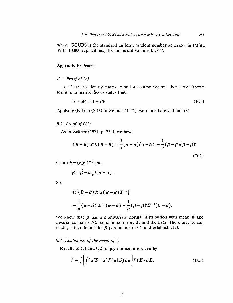
Appendix B: Proofs
B.1. Proof of (8)
Let I be the identity matrix, a and b column vectors, then a well-knownformula in matrix theory states that:
Il+ab'!= 1 +a'b. (B.1)
Applying (B.1) to (8.43) of Zellner (1971), we immediately obtain (8).
B.2. Proofof (12)
As in Zellner (1971, p. 232), we have
where b = (r;rp)-l and
So,
We know that fJ has a multivariate normal distribution with mean ji andcovariance matrix hI, conditional on lX, I, and the data. Therefore, we canreadily integrate out the fJ parameters in (7) and establish (12).
B.3. Evaluation of the mean of )..
Results of (7) and (12) imply the mean is given by
A All - -(B -B)'X'X(B -B) = ;(0'-&)(0'-&)' + b(/3 -fJ)(/3 -/3)',
(B.2)
ji =p - br;l(a - a).
tr[ (B - B)'X'X(B - B)I-I]
1 1 - -= ;(a-a)'X-I(a-a) + b(/3 -/3)'X-I(/3 -/3).
[f (a'X-la)P(aIX) da]X=f (B.3)P(I) dI,
252
where P(aII) is the multivariate normal density with mean Ii and covari-ance matrix aI, P(I) is the inverted Wishart density, i.e., the one obtainedfrom the right-hand side of (7) by adding a constant. To evaluate (B.3), wemake the following transformation of the parameters:
a=(a2')1/28+«.. (B.4)
Then 8 will follow the standard multivariate normal distribution, and
a'2'-la=aO'8 + 2al/2«.'2'-1/28 +«"2'-1«..
Therefore, after performing the integration in the a or 8 space in (B.3), wehave the result
"'~-I" + ATa a IVa.
Now let A=I-1, then A has a Wishart density W(S-I,T-2,N) [seeZellner (1971, app. B)].
Apply the moments results of a Wishart distribution to
A,~-lAa.. a=
We immediately obtain (13), that is:
X =Na +«'1;-1«.
ReferencesAnderson, Theodore W., 1984, An introduction to multivariate statistical analysis, 2nd ed.
(Wiley, New York, NY).Barnett, William A., John Geweke, and Piyu Yue, 1988, Semiparametric Bayesian estimation of
the asymptotically ideal model: The AIM demand system, Unpublished working paper (DukeUniversity, Durham, NC).
Black, Fischer, 1972, Capital market equilibrium with restricted borrowing, Journal of Business45, 444-454.
Box, George E.P. and George C. Tiao, 1965, Multiparameter problems from a Bayesian point ofview, Annals of Mathematical Statistics 36, 1468-1482.
Boyle, Phelim P., 1977, Options: A Monte Carlo approach, Journal of Financial Economics 4,323-338.
Breeden, Douglas T., 1979, An intertemporal asset pricing model with stochastic consumptionand investment opportunities, Journal of Financial Economics 7, 265-296.
Breeden, Douglas T., Michael R. Gibbons, and Robert H. Litzenberger, 1989, Empirical tests ofthe consumption based CAPM, Journal of Finance 44, 231-262.
Dickey, James M., 1971, The weighted likelihood ratio: Linear hypotheses on normal locationparameters, Annals of Mathematical Statistics 42, 204-223.
C.R. Harvey and G. Zhou, Bayesian inference in asset pricing test,~
(B.5)
C.R. Harvey and G. Zhou, Bayesian inference in asset pricing tests 253
Dybvig, Philip H., 1983, An explicit bound on individual assets' deviations from APT pricing in afinite economy, Journal of Financial Economics 12, 483-496.
Ferson, Wayne E. and Campbell R. Harvey, 1991, The variation of economic risk premiums,Unpublished working paper (Duke University, Durham, NC), forthcoming in the Journal ofPolitical Economy.
Gallant, A. Ronald and John F. Monahan, 1985, Explicit infinite dimensional Bayesian analysisof production technologies, Journal of Econometrics 30, 171-202.
Geisser, Seymour and J. OJrnfield, 1963, Posterior distributions for multivariate normal parame-ters, Journal of the Royal Statistical Society B 25, 368-376.
Geweke, John, 1986, Exact inference in the inequality constrained normal linear regressionmodel, Journal of Applied Econometrics 1, 127-141.
Geweke, John, 1988, Antithetic acceleration of Monte Carlo integration in Bayesian inference,Journal of Econometrics 38, 73-90.
Geweke, John, 1989, Bayesian inference in econometric models using Monte Carlo integration,Econometrica 57,1311-1339.
Gibbons, Michael R., 1982, Multivariate tests of financial models: A new approach, Journal ofFinancial Economics 10,3-27.
Gibbons, Michael R., Stephen A. Ross, and Jay Shanken, 1989, A test of the efficiency of a givenportfolio, Econometrica 57,1121-1152.
Grinblatt, Mark and Sheridan Titman, 1983, Factor pricing in a finite economy, Journal ofFinancial Economics 12,497-508.
Hull, John and Alan White, 1987, The pricing of options on assets with stochastic volatilities,Journal of Finance 42, 281-300.
Jeffreys, Harold, 1961, The theory of probability (Oxford University Press, Oxford).KJoek, Teun and Herman K. van Dijk, 1978, Bayesian estimates of equation system parameters:
An application of integration by Monte Carlo, Econometrica 46, 1-20.Krishnaiah, Paruchuri R., 1980, OJmputations of some multivariate distributions, in: P.R.
Krishnaiah, ed., Handbook of statistics (North-Holland, Amsterdam).Lintner John, 1965, The valuation of risk assets and the selection of risky investments in stock
portfolios and capital budgets, Review of Economics and Statistics 47, 13-37.Long, John B. Jr., 1974, Stock prices, inflation, and the term structure of interest rates, Journal
of Financial Economics 1, 131-170.MacKinlay, A. Craig, 1987, On multivariate tests of the capital asset pricing model, Journal of
Financial Economics 18,341-372.McCulloch, Robert and Peter E. Rossi, 1988, Testing the arbitrage pricing theory: Predictive
distributions, posterior distributions and odds ratios, Unpublished working paper (Universityof Chicago, Chicago, IL).
McCulloch, Robert and Peter E. Rossi, 1989a, A Bayesian approach to testing arbitrage pricingtheory, Unpublished working paper (University of Chicago, Chicago, IL), forthcoming in theJournal of Econometrics.
McCulloch, Robert and Peter E. Rossi, 1989b, Posterior, predictive, and utility-based ap-proaches to testing the arbitrage pricing theory, Unpublished working paper (University ofChicago, Chicago, IL).
Merton, Robert C., 1973, An intertemporal capital asset pricing model, Econometrica 41,867-887.
Press, S. James, 1982, Applied multivariate analysis: Using Bayesian and frequentist methods ofinference, 2nd ed. (Krieger, Malibar, FL).
Richard, Jean-Francois and Mark F.J. Steel, 1988, Bayesian analysis of systems of seeminglyunrelated regression equations under a recursive extended natural conjugate prior density,Journal of Econometrics 38, 7-37.
Ross, Stephen A., 1976, The arbitrage theory of capital asset pricing, Journal of EconomicTheory 13, 341-360.
Rossi, Peter E., 1980, Testing hypotheses in multivariate regression: Bayes vs. non-Bayesprocedures, Unpublished working paper (University of Chicago, Chicago, IL).
Rubinstein, Mark, 1976, The valuation of uncertain income streams and the pricing of options,Bell Journal of Economics 7, 407-425.
Scheffe, Henry, 1977, A note on the reformulation of the S-method of multiple comparison,Journal of the American Statistical Association 72, 143-144.
254
Shanken, Jay, 1985, Multivariate tests of the zero-beta CAPM, Journal of Financial Economics14, 327-348.
Shanken, Jay, 1986, Testing portfolio efficiency when the zero-beta rate is unknown: A note,Journal of Finance 41, 269-276.
Shanken, Jay, 1987a, Multivariate proxies and asset pricing relations: Living with the Rollcritique, Journal of Financial Economics 18,91-110.
Shanken, Jay, 1987b, A Bayesian approach to testing portfolio efficiency, Journal of FinancialEconomics 19, 195-216.
Shanken, Jay, 1990, Intertemporal asset pricing: An empirical investigation, forthcoming in theJournal of Econometrics.
Sharpe, William, 1964, Capital asset prices: A theory of market equilibrium under conditions ofrisk, Journal of Finance 19,425-442.
Sharpe, William, 1982, Factors in New York Stock Exchange security returns, 1931-1979,Journal of Portfolio Management 8, 5-19.
Stambaugh, Robert F., 1982, On the exclusion of assets from tests of the two parameter mode!:A sensitivity analysis, Journal of Financial Economics 10,237-268.
Zellner, Arnold, 1971, An introduction to Bayesian inference in econometrics (Wiley, New York,NY).
Zellner, Arnold, A. Luc Bauwens and Herman K. van Dijk, 1988, Bayesian specification analysisand estimation of simultaneous equation models using Monte Carlo methods, Journal ofEconometrics 38, 39-72.
Zellner, Arnold and Aloysius Siow, 1980, Posterior odds ratios for selected regression hypothe-ses, in: J.M. Bernardo, D.V. Lindley, and A.F.M. Smith, eds., Bayesian analysis: Proceedingsof the first international meeting (University Press, Spain).
C.R. Harvey and G. Zhou, Bayesian inference in asset pricing tests