27
Bayesian Learning Rong Jin
| Date post: | 31-Dec-2015 |
| Category: |
Documents |
| Upload: | felicia-beach |
| View: | 35 times |
| Download: | 0 times |

Bayesian Learning
Rong Jin

Outline MAP learning vs. ML learning Minimum description length principle Bayes optimal classifier Bagging

Maximum Likelihood Learning (ML) Find the model that best model by maximizing the log-
likelihood of the training data Logistic regression
Parameters are found by maximizing the likelihood of training data
1 2
1( | ; )
1 exp ( )
{ , ,..., , }m
p y xy x w c
w w w c
* *
1, ,
1, max ( ) max log
1 exp
ntrain iw c w c
w c l Dy x w c

Maximum A Posterior Learning (MAP) In ML learning, models are solely determined by the training examples Very often, we have prior knowledge/preference about parameters/models ML learning is unable to incorporate the prior knowledge/preference on
parameters/models Maximum a posterior learning (MAP)
Knowledge/preference about parameters/models are incorporated through a prior
* arg max Pr( | )D
Prior for parameters
Pr( )

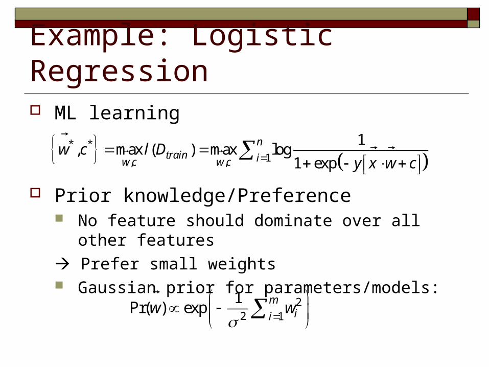
Example: Logistic Regression ML learning
Prior knowledge/Preference No feature should dominate over all other features
Prefer small weights Gaussian prior for parameters/models:
* *
1, ,
1, max ( ) max log
1 exp
ntrain iw c w c
w c l Dy x w c
22 1
1Pr( ) exp
mii
w w
Example: Logistic Regression ML learning
Prior knowledge/Preference No feature should dominate over all other features
Prefer small weights Gaussian prior for parameters/models:
* *
1, ,
1, max ( ) max log
1 exp
ntrain iw c w c
w c l Dy x w c
22 1
1Pr( ) exp
mii
w w

Example (cont’d) MAP learning for logistic regression
Compared to regularized logistic regression
* *
,
221 1
,
, arg max Pr( | , ) Pr( , )
arg max log Pr( | , ) log Pr( , )
1 1arg max log
1 exp
w c
n mii i
w c
w c D w c w c
D w c w c
wy x w c
21 1
1( ) log
1 exp ( )N m
reg train ii il D s w
y c x w

Minimum Description Length Principle Occam’s razor: prefer the simplest hypothesis
Simplest hypothesis hypothesis with shortest description length
Minimum description length Prefer shortest hypothesis
LC (x) is the description length for message x under coding scheme c
1 2arg min ( ) ( | )MDL C C
h Hh L h L D h
# of bits to encode hypothesis h
# of bits to encode data D given h
Complexity of Model
# of Mistakes

Minimum Description Length Principle
1 2arg min ( ) ( | )MDL C C
h Hh L h L D h
D
Sender ReceiverSend only D ?
Send only h ?
Send h + D/h ?

Example: Decision Tree H = decision trees, D = training data labels LC1
(h) is # bits to describe tree h
LC2(D|h) is # bits to describe D given tree h
Note LC2(D|h)=0 if examples are classified
perfectly by h. Only need to describe exceptions
hMDL trades off tree size for training errors

MAP vs. MDL MAP learning:
Fact from information theory The optimal (shortest expected coding length) code for an
event with probability p is –log2p Interpret MAP using MDL principle
2 2
2 2
arg max Pr( | ) Pr( ) arg max log Pr( | ) log Pr( )
arg min log Pr( ) log Pr( | )
MAPh H h H
h H
h D h h D h h
h D h
1 2arg min ( ) ( | )MDL C C
h Hh L h L D h
Description length of h under optimal coding
Description length of exceptions under optimal coding
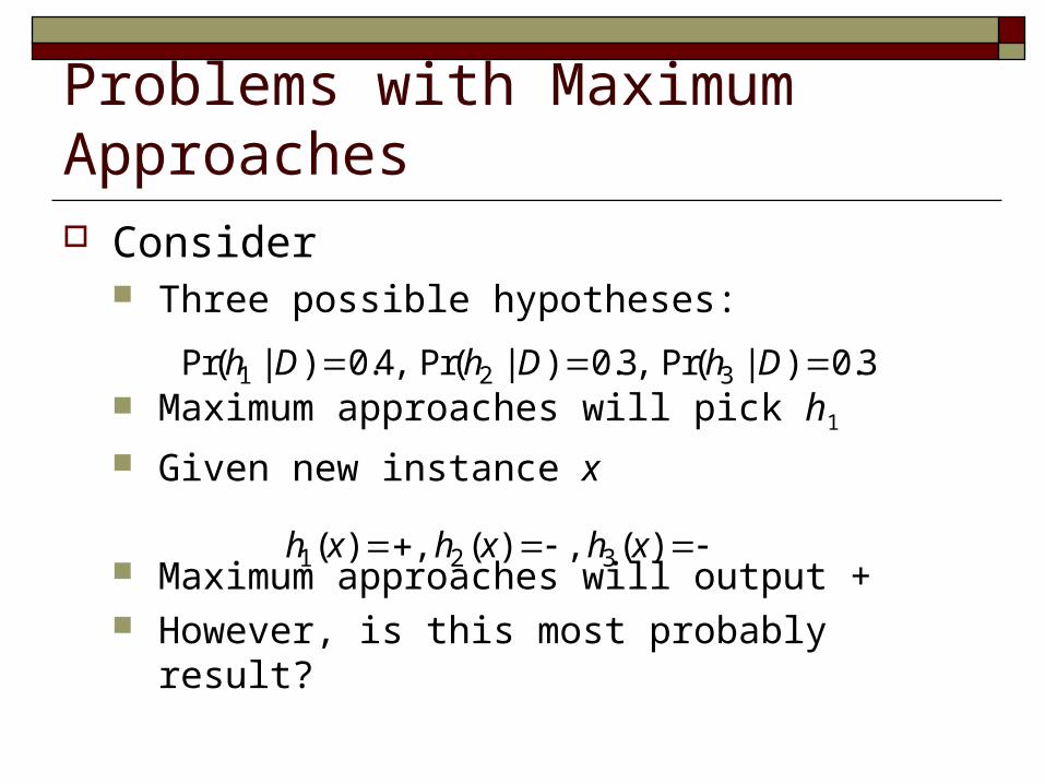
Problems with Maximum Approaches Consider
Three possible hypotheses:
Maximum approaches will pick h1
Given new instance x
Maximum approaches will output + However, is this most probably result?
1 2 3Pr( | ) 0.4, Pr( | ) 0.3, Pr( | ) 0.3h D h D h D
1 2 3( ) , ( ) , ( )h x h x h x

Bayes Optimal Classifier (Bayesian Average) Bayes optimal classification:
Example:
The most probably class is -
*( ) arg max Pr( | )Pr( | , )c h H
c x h D c h x
1 1 1
2 2 2
3 3 3
Pr( | ) 0.4, Pr( | , ) 1, Pr( | , ) 0
Pr( | ) 0.3, Pr( | , ) 0, Pr( | , ) 1
Pr( | ) 0.3, Pr( | , ) 0, Pr( | , ) 1
Pr( | )Pr( | , ) 0.4, Pr( | )Pr( | , ) 0.6h h
h D h x h x
h D h x h x
h D h x h x
h D h x h D h x

When do We Need Bayesian Average? Bayes optimal classification
*( ) arg max Pr( | )Pr( | , )c h H
c x h D c h x
When do we need Bayesian average?Multiple mode caseOptimal mode is flat
When NOT Bayesian Average?Can’t estimate Pr(h|D) accurately
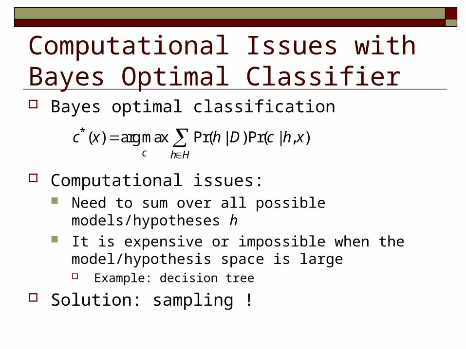
Computational Issues with Bayes Optimal Classifier Bayes optimal classification
Computational issues: Need to sum over all possible models/hypotheses h It is expensive or impossible when the model/hypothesis
space is large Example: decision tree
Solution: sampling !
*( ) arg max Pr( | )Pr( | , )c h H
c x h D c h x
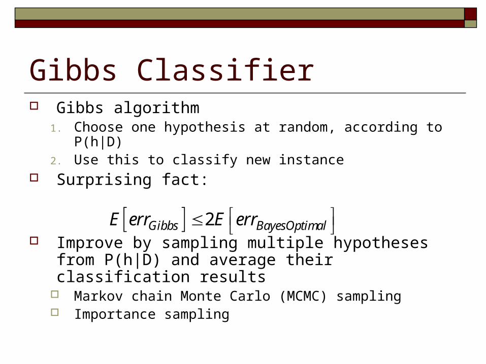
Gibbs Classifier Gibbs algorithm
1. Choose one hypothesis at random, according to P(h|D)2. Use this to classify new instance
Surprising fact:
Improve by sampling multiple hypotheses from P(h|D) and average their classification results
Markov chain Monte Carlo (MCMC) sampling Importance sampling
2Gibbs BayesOptimalE err E err

Bagging Classifiers In general, sampling from P(h|D) is difficult
because1. P(h|D) is rather difficult to compute
Example: how to compute P(h|D) for decision tree?
2. P(h|D) is impossible to compute for non-probabilistic classifier such as SVM
3. P(h|D) is extremely small when hypothesis space is large Bagging Classifiers:
Realize sampling P(h|D) through a sampling of training examples
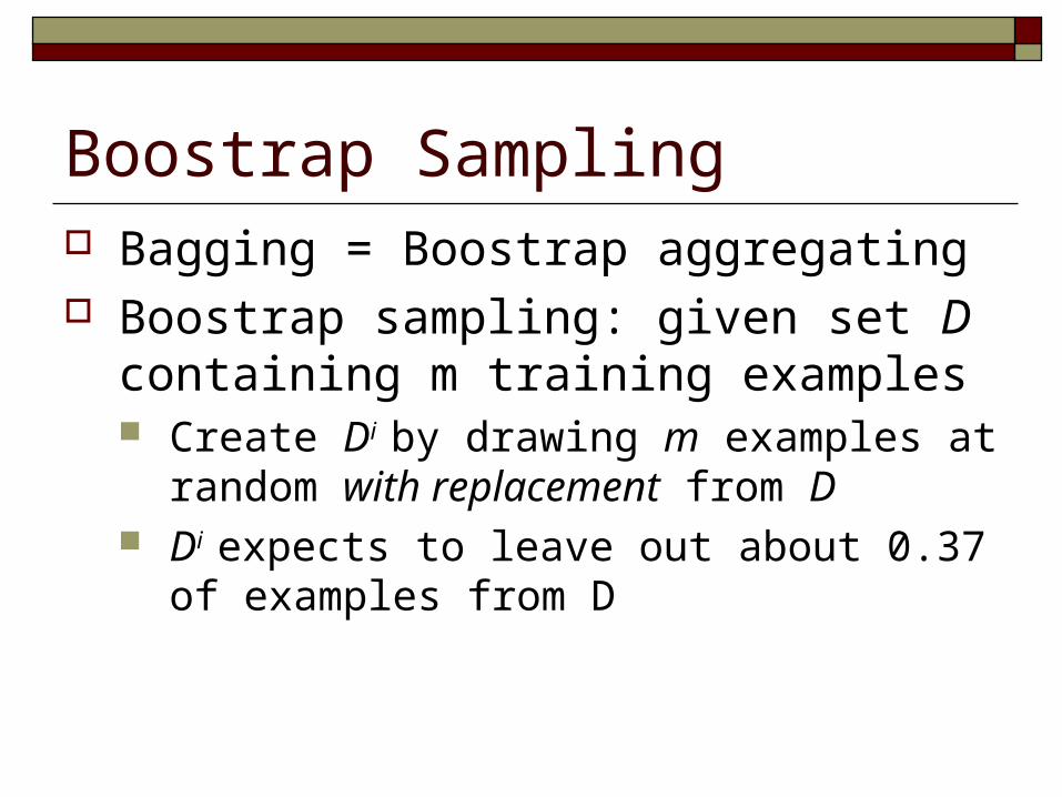
Boostrap Sampling Bagging = Boostrap aggregating Boostrap sampling: given set D containing m
training examples Create Di by drawing m examples at random with
replacement from D Di expects to leave out about 0.37 of examples
from D
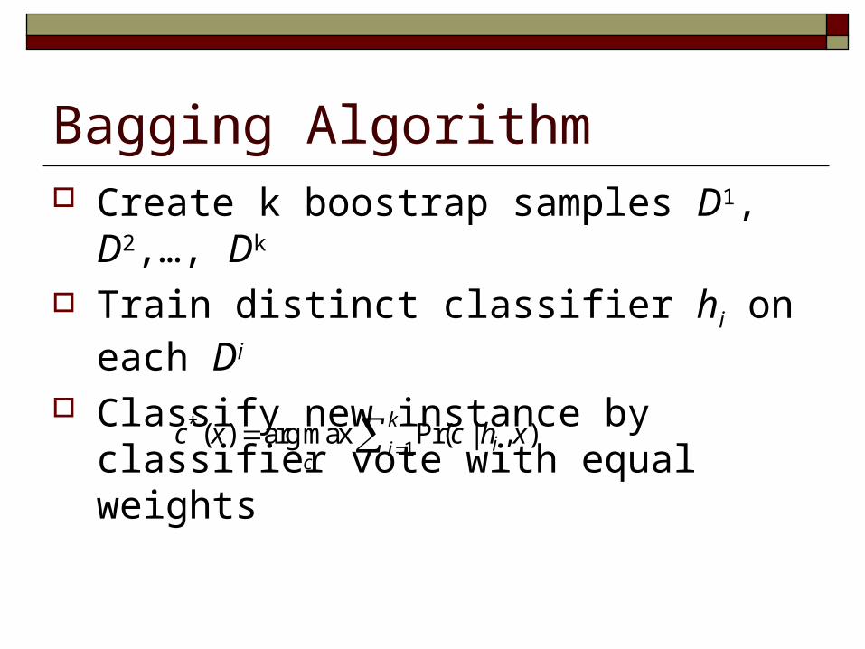
Bagging Algorithm Create k boostrap samples D1, D2,…, Dk
Train distinct classifier hi on each Di
Classify new instance by classifier vote with equal weights
*1
( ) arg max Pr( | , )k
iic
c x c h x

Bagging Bayesian Average
P(h|D)
Bayesian Average
…h1 h2 hk
Sampling
Pr( | , )iic h x
D
Bagging
…
D1 D2 Dk
Boostrap Sampling
Pr( | , )iic h x
h1 h2 hk
Boostrap sampling is almost equivalent to sampling from posterior P(h|D)

Empirical Study of Bagging Bagging decision trees
Boostrap 50 different samples from the original training data
Learn a decision tree over each boostrap sample
Predicate the class labels for test instances by the majority vote of 50 decision trees
Bagging decision tree performances better than a single decision tree
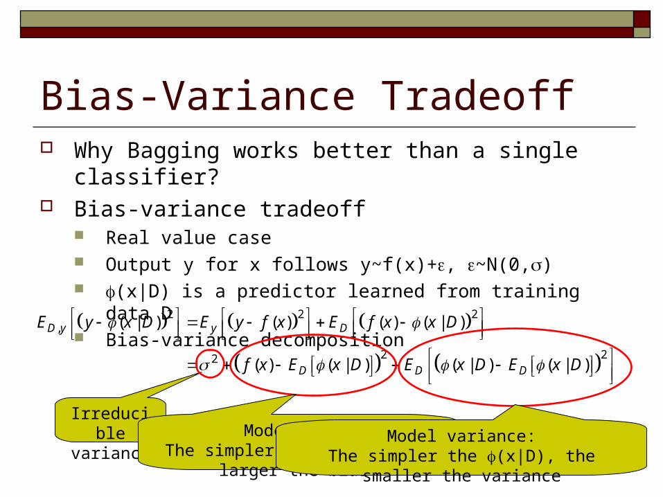
Why Bagging works better than a single classifier? Bias-variance tradeoff
Real value case Output y for x follows y~f(x)+, ~N(0,) (x|D) is a predictor learned from training data D Bias-variance decomposition
Bias-Variance Tradeoff
2 2 2,
2 22
( | ) ( ) ( ) ( | )
( ) ( | ) ( | ) ( | )
D y y D
D D D
E y x D E y f x E f x x D
f x E x D E x D E x D
Irreducible variance Model bias:
The simpler the (x|D), the larger the bias Model variance:
The simpler the (x|D), the smaller the variance

Bias-Variance Tradeoff
True Model
Fit with Complicated Models
Small model bias
Large model variance
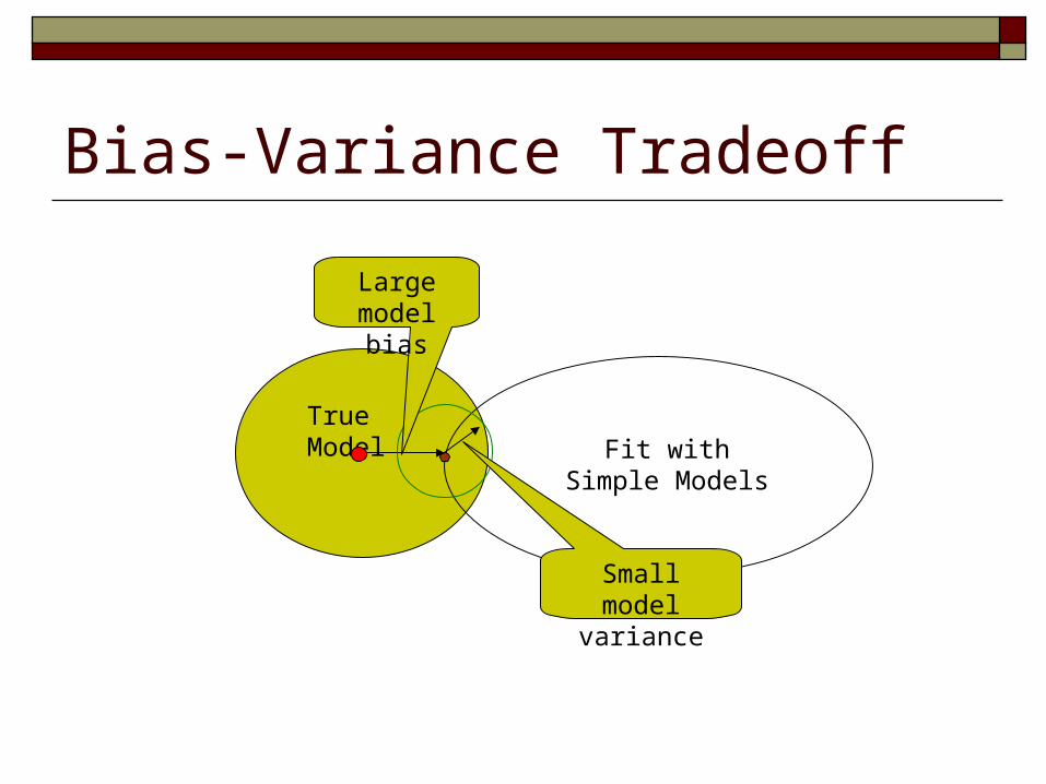
Bias-Variance Tradeoff
True ModelFit with Simple
Models
Large model bias
Small model variance
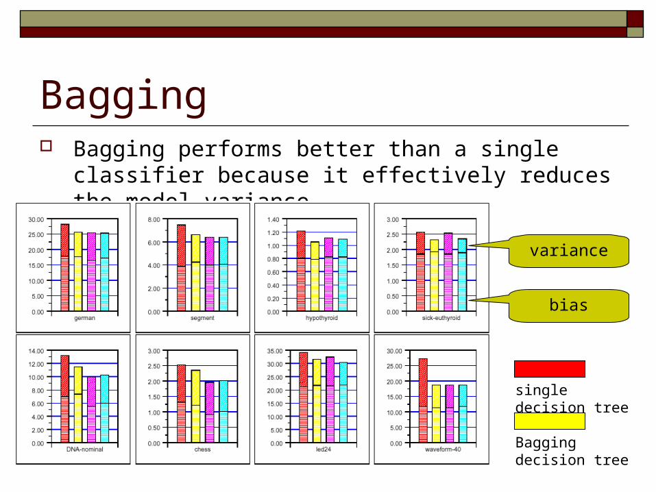
Bagging Bagging performs better than a single classifier because it
effectively reduces the model variance
single decision tree
Bagging decision tree
bias
variance


