Bayesian Networks for Raster Data (BayNeRD): Plausible

Remote Sens. 2013, 5, 5999-6025; doi:10.3390/rs5115999

Remote Sensing ISSN 2072-4292

www.mdpi.com/journal/remotesensing

Article

Bayesian Networks for Raster Data (BayNeRD): Plausible Reasoning from Observations

Marcio Pupin Mello 1,2,3,*, Joel Risso 4, Clement Atzberger 2, Paul Aplin 5, Edzer Pebesma 3,

Carlos Antonio Oliveira Vieira 6 and Bernardo Friedrich Theodor Rudorff 4

1 Remote Sensing Division (DSR), National Institute for Space Research (INPE),

São José dos Campos, SP 12227-010, Brazil 2 Institute of Surveying, Remote Sensing and Land Information (IVFL), University of Natural

Resources and Life Sciences (BOKU), Vienna 1190, Austria; E-Mail: [email protected] 3 Institute for Geoinformatics (ifgi), University of Muenster, D-48151 Muenster, Germany;

E-Mail: [email protected] 4 Agrosatélite Applied Geotechnology, Florianópolis, SC 88032-005, Brazil;

E-Mails: [email protected] (J.R.); [email protected] (B.F.T.R.) 5 School of Geography, University of Nottingham, Nottingham NG7 2RD, UK;

E-Mail: [email protected] 6 Geosciences Department, Federal University of Santa Catarina (UFSC), Florianópolis,

SC 88040-900, Brazil; E-Mail: [email protected]

* Author to whom correspondence should be addressed; E-Mail: [email protected];

Tel.: +55-12-3208-6465; Fax: +55-12-3208-6488.

Received: 4 September 2013; in revised form: 8 November 2013 / Accepted: 11 November 2013 /

Published: 15 November 2013

Abstract: This paper describes the basis functioning and implementation of a computer-aided

Bayesian Network (BN) method that is able to incorporate experts’ knowledge for the

benefit of remote sensing applications and other raster data analyses: Bayesian Network for

Raster Data (BayNeRD). Using a case study of soybean mapping in Mato Grosso State,

Brazil, BayNeRD was tested to evaluate its capability to support the understanding of a

complex phenomenon through plausible reasoning based on data observation. Observations

made upon Crop Enhanced Index (CEI) values for the current and previous crop years, soil

type, terrain slope, and distance to the nearest road and water body were used to calculate

the probability of soybean presence for the entire Mato Grosso State, showing strong

adherence to the official data. CEI values were the most influencial variables in the

calculated probability of soybean presence, stating the potential of remote sensing as a

OPEN ACCESS

Remote Sens. 2013, 5 6000

source of data. Moreover, the overall accuracy of over 91% confirmed the high accuracy of

the thematic map derived from the calculated probability values. BayNeRD allows the

expert to model the relationship among several observed variables, outputs variable

importance information, handles incomplete and disparate forms of data, and offers a basis

for plausible reasoning from observations. The BayNeRD algorithm has been implemented

in R software and can be found on the internet.

Keywords: Belief network; weights of evidence; remote sensing; ancillary data;

soybean mapping

1. Introduction

Understanding complex phenomena in the field of Earth observation sciences represents a

considerable challenge for scientific analysis [1,2]. Regarding investigation of large scale phenomena,

great progress has been achieved through recent advances in spaceborne remote sensing data

acquisition [3], together with the availability of high performance computing for remotely sensed data

analysis [4]. To Lu & Weng [5], the most important factors driving the success of an inference based

on remotely sensed data are: (i) the availability of high-quality observations (e.g., accurate imagery

corrected for atmospheric effects and ancillary data such as topography, soil, road, and census data);

(ii) the design of a suitable analytical procedure; and (iii) the analyst’s skills and knowledge. However,

some phenomena are often too complex to be investigated by conventional methods [6], demanding

new computer aided methods to help characterize phenomena through plausible reasoning inferences

based on consistent data observations (i.e., evidence).

Interactions of probabilities have been identified as the most promising way for a computer to effect

plausible reasoning [7]. The Bayes’ theorem updates the knowledge (prior probability) of a specific

event in the light of new/additional evidence (conditional probabilities), allowing one to have a

plausible reasoning based on a degree of belief (posteriori probability) [8]. Thus, observations made

upon variables that are related to a particular phenomenon can be used to develop plausible reasoning

about the phenomenon, its causes, and consequences [7]. When the number of variables increases or

even when the complexity of the interactions among the variables involved in a phenomenon rises, the

Bayesian Network (BN) is a representation suited to model and handle such tasks [9,10].

Neapolitan [11] defines BNs as graphical structures for representing the probabilistic relationship

among a set of variables via a Directed Acyclic Graph (DAG), and for calculating probabilistic

inference with those variables. BNs can also be defined as representational structures that are meant to

organize one’s knowledge about a particular phenomenon into a coherent whole [12]. The advantages

of BNs are that they: (i) can deal with a large number of variables and can also handle incomplete data

sets (i.e., missing data); (ii) can deal with both numeric and categorical data simultaneously; (iii) are

able to incorporate experts’ knowledge via a participatory modeling procedure of causal relationships;

and (iv) are easy to understand and visualize through DAGs [13,14]. Notwithstanding these advantages,

Aguilera et al. [15] pointed out that BNs have rarely been used in the field of Earth observation

sciences and remote sensing, and their potential is, as yet, largely unexploited.


Although researchers have made substantial advances in developing the theory and application of

BNs [11], the actual use of these networks often remains a difficult and time-consuming task [15].

In the Earth observation sciences, where investigations commonly involve numerous layers of data

(e.g., maps and images), analysis can be difficult due to the need to know both the relationships among

the variables (i.e., conditional (in)dependences) and their probability functions. In addition, tasks can

be time-consuming because they are typically performed manually. Until now, only a limited number

of computer aided methods have been implemented. Therefore, there is potential for the use of

probability theory as a basis for computer aided plausible reasoning, and BNs as a tool for representing

and computing probabilistic beliefs in the field of Earth observation sciences [14]. Moreover, there is

demand for the development and implementation of computer aided methods that offer a basis for

Earth observation science researchers to understand and model phenomena through plausible reasoning

inferences based on data observations [15].

The aim of this paper is to describe, implement and test a computer aided BN method that is able to

incorporate experts’ knowledge for the benefit of remote sensing applications and other raster data

analyses. The freely available algorithm is named Bayesian Networks for Raster Data (BayNeRD).

Following development of the approach, BayNeRD was tested on a case study for soybean identification

and mapping in Mato Grosso State, Brazil. The test enabled evaluation of the capability of

BayNeRD to support the understanding of a complex phenomenon through plausible reasoning based

on data observation.

2. Bayesian Networks

A BN for a set of n variables consists of: (i) a network structure, graphically represented by a DAG

with nodes and arcs, that encodes a set of conditional (in)dependence assertions about the variables;

and (ii) a set of probability functions associated with each variable [11]. We use upper-case letters

(e.g., V1, Vn) to denote both a variable and its corresponding node, and the same but lower-case letters

(e.g., v1, vn) to denote the state or value (defining a particular instantiation) of the variable. Then, the

joint probability distribution for any particular instantiation of all n variables in a BN is given by: ( = ,… , = ) = ( = |Φ = ) (1)

where vi represents the instantiation of variable Vi and ϕi represents the instantiation of its parents Φi,

with i varying from 1 to n. Parent variables are those whose instantiations directly influence other,

descendent variables. The arcs (represented by arrows in the DAG) encode the conditional dependencies

(i.e., which variables are parent/descendant of other variables) [9,11]. The joint probability of any

instantiation of all the variables in a BN can be computed as the product of only n probabilities. Thus,

we can determine any probability of the form: ( | , … , ) (2)

where Vi are sets of variables with known values (vi, i.e., instantiated variables). This ability to compute

posterior probabilities given some evidence is called inference. In the case of using Equation (2) for

inferences about certain phenomena using BayNeRD, we named the variable that represents the


phenomenon as the target variable and the variables that can be used to describe an outline of the

phenomenon as context variables (i.e., those variables that are somehow related to the phenomenon).

To illustrate the concept, suppose we are interested in inferring soybean occurrence based on

observations of other variables. It is well known that soybean plantations have certain peculiarities [16],

such as: (i) it is preferably not sown in areas with steep terrain slope because mechanization may be

hindered; and (ii) it is preferably sown in soils that are more suitable for agricultural cultivation (that

we will refer as soil aptitude). Then, soybean occurrence (S) is the target variable and can be represented

by a thematic map with the classes soybean and non-soybean, that imply soybean presence (S = 1) and

soybean absence (S = 0), respectively. On the other hand, terrain slope (T) and soil aptitude (A) could

be, in our example, two context variables. As we are interested to infer about S, in this example,

Equation (2) becomes: ( | , ) (3)

Indeed, T and A directly influence S and, thus, are said to be parents of S. Moreover, as soil

formation processes are strongly influenced by terrain slope [17], T also influences A and, therefore,

T is also a parent of A. These (in)dependence relationships among the variables are represented by a

DAG as shown in Figure 1.

Figure 1. Directed Acyclic Graph (DAG) representing a hypothetical BN graphical model

where the target variable soybean occurrence (S) is influenced by two context variables:

terrain slope (T) and soil aptitude (A). Since soil formation processes are strongly influenced

by terrain slope, T is also parent of A. Variables are represented by nodes and dependences

are represented by arcs between pairwise nodes.

The representation of conditional (in)dependencies is the essential function of BNs. For each node

in a BN structure, there is a conditional-probability function that relates this node to its immediate

parents. If a node has no parents (e.g., T) then a prior-probability function is specified [10]. Eventually,

once all probability functions are specified, it is possible to compute the probability of soybean

presence (S = 1) in a certain area based on the observed values for both T and A in the same area.

In practical terms, the definition of these probability functions is often the most complicated

part of BN modeling. However, the empirical Bayesian approach suggests that the functions can be

defined based on observations, i.e., from the data [18]. Mello et al. [19] proposed use of pixel counting

in discretized variables to compute probability functions in a BN when employing raster data

(described further).

Aware of the great demand for implemented computer algorithms to help handle and understand

phenomena in the field of Earth observation science, we implemented BayNeRD in R software [20].


The algorithm provides researchers a means of modeling any phenomenon of interest, whereby

plausible reasoning inferences are made based on observations stored in raster data format.

3. Framework of the Implemented BayNeRD Algorithm in R Software

R software was used to implement BayNeRD because it is a high-level language and environment

for data analysis and graphics. It is growing in popularity and uptake, and is freely available for the

research community [21]. Furthermore, among all packages already implemented in R software, there

are several developed for both handling spatial data [22] and computing Bayesian analysis [23],

especially catnet [24], which was designed for categorical BN.

The BayNeRD algorithm handles data in the GeoTIFF format, which has been widely used to

represent raster data with geographical coordinates. For use in BayNeRD all raster data (i.e., one

GeoTIFF representing each variable) must represent the same geographic area. Each GeoTIFF

corresponds to a variable (node) used in the BN model. These variables and their (in)dependence relations

are used to compute the probability functions.

3.1. Target Variable

The variable which directly represent the phenomenon is called the target variable. A GeoTIFF with

data representing the target variable as reference data for training must be provided. It is later used in

the definition of the probability functions. The GeoTIFF representing the target variable usually has

four labels representing the following thematic classes: (i) target presence observed; (ii) target absence

observed; (iii) missing data, i.e., no observations were made; and (iv) pixels outside the study area.

The latter is simply used to mask out any pixels that are outside the study area from any of the raster

data layers to be used in BayNeRD. Although reference data for training may contain more than these

four labels, it must have at least two: (i) and (ii). Thus, the target variable, represented in the general

model as Y, can be instantiated (Y = y) with y assuming either 1 for the target presence or 0 for the

target absence.

3.2. Context Variables

The context variables are those that exhibit any kind of relationship with the target variable (such as

terrain slope and soil aptitude, as previously discussed). Moreover context variables may exhibit

relationships among themselves, such as the terrain slope influencing the soil aptitude due to the

influence of slope in soil formation processes [17]. The context variables may contain any sort of

observations such as numerical values (e.g., terrain slope given in percentage) or categorical data

(e.g., thematic classes representing soil aptitude for agriculture cultivation). Moreover, the context

variables may also contain missing data.

One of the main difficulties of using BNs for real problems is the definition of the probability

functions of the model [18]. Therefore BayNeRD was developed to interact with the user to define,

through discretization processes, the probability functions of the model based on both observed data

and users’ knowledge about the phenomenon of interest. Discretization is the process of representing


(approximating) the observed values of a variable using discrete quantities (e.g., intervals, such as in

the process of drawing a histogram).

After the target variable has been entered as reference data for training and the context variables

have been read, the user will be able to design the BN graphical model.

3.3. Designing the Bayesian Network Graphical Model

To design the BN graphical model the user is asked about the (in)dependence relations among all

variables read (i.e., both target and context variables). As the dependencies are represented by arcs in a

DAG, BayNeRD asks whether an arc exists between pairwise variables. For example, if the terrain

slope (T) influences soil aptitude (A), and both T and A influence soybean occurrence (S), there will be

an arc from T to A, an arc from T to S, and another arc from A to S (see Figure 1). Once the graphical

representation of the BN model is defined stating the variables and their (in)dependence relations,

BayNeRD is able to compute the probability functions, which is done based on pixel counting in

discretized variables [19].

3.4. Discretization and Probability Functions

The discretization divides the range of the observed values for a variable into intervals and codes

the values in the variable according to which interval they belong. In BayNeRD the discretization is

based on choosing the number of intervals defined for each context variable and can be computed

following three implemented criteria: (i) equidistant intervals, where each interval has the same width;

(ii) quantiles, where each interval tends to have the same number of elements (i.e., pixels); and

(iii) manually defined intervals, where the user defines the upper and lower limits of each interval.

The discretization will have an impact on the computed probability functions. These probabilities

are computed through pixel counting according to both the (in)dependence relations defined in the BN

graphical model and the intervals defined in the discretization processes. Indeed, both the definition of

the BN graphical model and the discretization processes enable users to add their knowledge about the

phenomenon into the model. The more a data set is accurate, and a user is skilled in defining both BN

graphical model and interval limits during discretization processes, the more the data-based probability

functions computed are representative of the real probability functions [19].

Let us suppose that the terrain slope (T), which does not have parents in the designed BN model

represented in Figure 1, was discretized using four equidistant intervals between 0% and 100%. By

dividing the number of pixels with values lower than 25% by the total number of pixels observed for

the study area one can compute the probability for the first interval of the discretized T. The

probabilities for the remaining intervals of the discretized T are computed by pixel counting as

described above and the probabilities for all intervals must sum to 1. In the case of variables that have

parents, such as the soil aptitude (A), which is a descendent of T (Figure 1), BayNeRD uses the

intervals defined for T and the ones defined for A to compute the conditional probability function for A

in the BN model, also based on pixel counting [19].

The user should be sufficiently expert to define suitable discrete intervals for each context variable

so that all scenarios (i.e., combination of parents’ and variable’s intervals) have representative data to

compute probability functions, where a minimum user-defined quantity of pixels is considered as a


representative number. The process of computing the probability functions of the model is called

training, when BayNeRD defines the probability functions based on the observed values from the data

(i.e., by counting pixels). Using values of probability for plausible reasoning, BNs are able to infer

based on evidence (observed data). Indeed, once BayNeRD is trained, it is able to answer the question:

“what is the probability of target presence (e.g., soybean), given the observed values for the context

variables (e.g., terrain slope and soil aptitude)?” When the probability that answers this question is

calculated for every pixel in the entire study area, a Probability Image (PI) is formed.

3.5. Computing the Probability Image

The PI consists of a raster data (i.e., a matrix matching the same coordinates of the entered

reference data for training) where each pixel contains the probability of presence of the target given

the values observed (instantiations) for the input variables, i.e., ( = 1| = ,… , = ) (4)

If any context variable presents missing data for any specific pixel in the study area, it is considered

as “unobserved” in the model but Equation (4) is computed anyway taking into account all the

possibilities for that variable. It is also possible to find P(Y = 1) for pixels where no observation was

made for any context variable. In this case, the computed probability will be the marginal probability

for Y when Y = 1.

BayNeRD also allows the user to quantify the influence of each context variable on the probabilities

computed for the target variable. This is done through the Kullback-Leibler (KL) divergence, which is

a non-symmetric measure of the difference between two probability distributions [25]. Thus, it is

possible to measure how much V1, V2, … and Vn individually influence the probability computed for Y

by computing KL divergences between conditional and marginal probabilities in the BN model.

The main result of BayNeRD is the PI and it can be used in several applications. For example, the

PI can be used to generate a thematic map with classes target and non-target (e.g., soybean and

non-soybean) just by slicing the PI using a limiting probability value named the Target Probability

Value (TPV). Thus, by setting TPV at 50%, for instance, all pixels with values equal to or greater than

0.5 in the PI will be labeled as target and the remaining pixels (with values smaller than 0.5) will be

labeled as non-target. However, what if the best TPV was 70% instead of 50%? What about even 80%?

3.6. Selecting the Target Probability Value

Apart from a user-defined value, six criteria are implemented in BayNeRD to select the TPV which

best meets a chosen criterion, making use of available reference information (i.e., a reference data for

testing). These implemented criteria are: (i) nearest 100% sensitivity and 100% specificity point [26]

(these two indices account for the true positive rate and the true negative rate, respectively [27]);

(ii) minimum difference between sensitivity and specificity; (iii) highest overall accuracy index;

(iv) highest kappa index [28,29]; (v) most similar area (number of pixels) matching the reference data

for testing; and (vi) minimum difference between omission and commission errors [30].


4. Case Study of Soybean Mapping in Brazil: Materials and Research Methods

The case study involves soybean identification and mapping in Mato Grosso, which is a major

Brazilian soybean producer (about 30% of the total domestic production) and an important global hub

for tropical agricultural production [31]. Mato Grosso State is located in the Southwest of Legal

Brazilian Amazon, encompassing an area around 900,000 km2 [32]. Figure 2 shows the location of

Mato Grosso State, highlighting thirty 30 × 30 km plots (and the Landsat path/row covering them) of

reference data produced by Epiphanio et al. [33] for the crop year 2005/2006 (i.e., from August 2005

to July 2006) using visual interpretation of Landsat-5/TM images and field data. Additional data such

as indigenous lands, conservation units, mapped forests and floodplains were used to mask out areas of

no interest for mapping soybean (as will be described further).

Figure 2. Study area corresponding to Mato Grosso State, Brazil. The analysis was only

performed in areas that were not masked out.

Although Brazil is the second largest producer of soybean worldwide [34], the country does not

have a systematic nationwide mapping system for this oilseed. Tabulated agricultural statistics at

municipality level are only released with a delay of about two years after harvest. The absence of

timely and spatial data restricts investigations related to crop monitoring and forecast. It also hinders

the monitoring of the possible spread of this crop into new, sometimes environmentally-sensitive,

areas. As such, there is demand for the use of satellite sensor images as an accurate, efficient, timely,

and cost-effective way to monitor agricultural crops [35]. Several studies have demonstrated the value

of Landsat-like images to monitor agricultural crops in Brazil using visual interpretation [36,37] or

even automatically [38,39]. However, these methods have certain constraints, notably the limited

number of cloud-free images that are routinely acquired during the crop cycle [40,41]. Alternatively,

multitemporal approaches using Moderate Resolution Imaging Spectroradiometer (MODIS) time


series images have been successfully used to monitor soybean plantations in tropical regions such as

Mato Grosso, as the one to two day temporal-resolution of MODIS increases the chance of obtaining

cloud-free images [42–44].

In addition to remotely sensed spectral and temporal information, several other context variables are

closely related with soybean occurrence in a given field (e.g., soil type and infrastructure facilities) [16].

In the present study, this information is combined within a BN structure to optimize soybean identification

and mapping. Figure 3 shows a flowchart summarizing the research material and methods employed in

the soybean mapping case study application of BayNeRD.

Figure 3. Summary of the procedures used in the case study of applying BayNeRD to

identify soybean plantations in Mato Grosso State, Brazil. Table 1 provides a description of

the variables used.

In summary, six context variables and a reference thematic map were used as inputs in BayNeRD,

where a BN model was defined based on experts’ knowledge. Probability functions were computed

based on pixel counting of discretized variables, allowing BayNeRD to compute the PI, which was

eventually used to produce a thematic map of soybean occurrence over the study area. This thematic

map was then assessed using reference data. The following subsections describe the research materials

and methods in detail.

4.1. Variables

All variables used in this case study, each represented by a raster GeoTIFF, were resampled to

match the grid of the MODIS vegetation indices product (MOD13Q1), with a nominal spatial

resolution of 250 × 250 m [45].

Next, two classes of variables were entered:


(1) Target variable—soybean occurrence (S) corresponding to the studied phenomenon,

represented by a thematic map with four classes for the crop year 2005/2006: (i) target

presence observed (i.e., soybean); (ii) target absence observed (i.e., non-soybean); (iii) missing

data (i.e., no observations); and (iv) pixels outside the study area. This thematic map, produced

by Epiphanio et al. [33], was used as a reference in this study. In the BayNeRD modelling,

S = s, where s = 1 for soybean presence and s = 0 for soybean absence. Two thirds of the pixels

in each of the thematic class soybean and non-soybean were randomly selected from the

reference map to compose the reference data for training. The remaining third of the reference

map pixels was set aside to be used for accuracy assessment (reference data for testing).

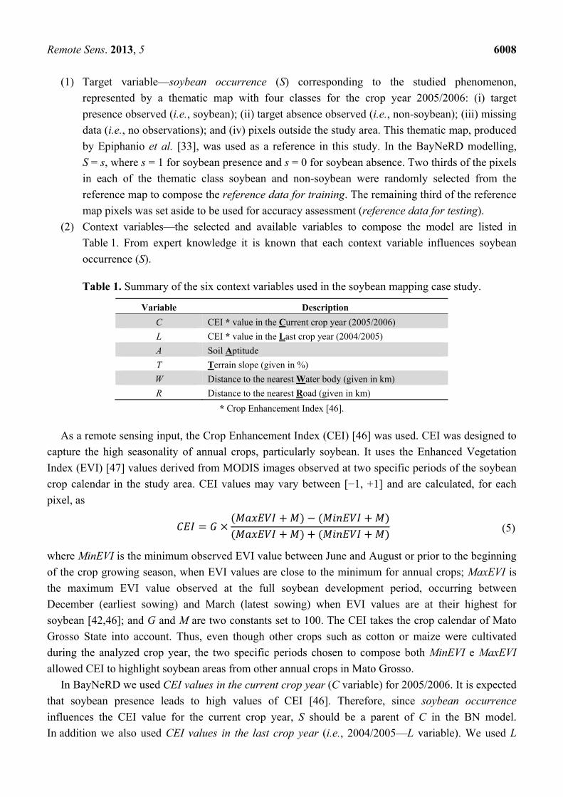
(2) Context variables—the selected and available variables to compose the model are listed in

Table 1. From expert knowledge it is known that each context variable influences soybean

occurrence (S).

Table 1. Summary of the six context variables used in the soybean mapping case study.

Variable Description

C CEI * value in the Current crop year (2005/2006)

L CEI * value in the Last crop year (2004/2005)

A Soil Aptitude

T Terrain slope (given in %)

W Distance to the nearest Water body (given in km)

R Distance to the nearest Road (given in km)

* Crop Enhancement Index [46].

As a remote sensing input, the Crop Enhancement Index (CEI) [46] was used. CEI was designed to

capture the high seasonality of annual crops, particularly soybean. It uses the Enhanced Vegetation

Index (EVI) [47] values derived from MODIS images observed at two specific periods of the soybean

crop calendar in the study area. CEI values may vary between [−1, +1] and are calculated, for each

pixel, as = × ( + ) − ( + )( + ) + ( + ) (5)

where MinEVI is the minimum observed EVI value between June and August or prior to the beginning

of the crop growing season, when EVI values are close to the minimum for annual crops; MaxEVI is

the maximum EVI value observed at the full soybean development period, occurring between

December (earliest sowing) and March (latest sowing) when EVI values are at their highest for

soybean [42,46]; and G and M are two constants set to 100. The CEI takes the crop calendar of Mato

Grosso State into account. Thus, even though other crops such as cotton or maize were cultivated

during the analyzed crop year, the two specific periods chosen to compose both MinEVI e MaxEVI

allowed CEI to highlight soybean areas from other annual crops in Mato Grosso.

In BayNeRD we used CEI values in the current crop year (C variable) for 2005/2006. It is expected

that soybean presence leads to high values of CEI [46]. Therefore, since soybean occurrence

influences the CEI value for the current crop year, S should be a parent of C in the BN model.

In addition we also used CEI values in the last crop year (i.e., 2004/2005—L variable). We used L


because soybean plantations in Mato Grosso present spatially persistent characteristics over time,

i.e., if soybean is sown on a given plot in a given year it is likely that soybean will be sown on the

same plot in the following crop year [48]. Thus, L should be a parent of S in the BN model.

Soybean occurrence is also influenced by soil type [48], represented here by the variable soil aptitude

(A). To set the soil aptitude for soybean production, we used a thematic soil map (1:250,000 scale)

provided by the Secretariat of Planning and Coordination of Mato Grosso State (SEPLAN-MT) [49].

This map was produced within the scope of an ecological-economic zoning project, according to the

Brazilian System of Soil Classification [50,51]. Originally, the soil map contained 26 classes (types of

soil), which were pooled into two aptitude classes, low and high, defined by skilled soil experts

according to soil properties such as soil composition, water holding capacity, and fertility. The low

aptitude class encompasses the following soils: rock outcrops, gleysols, lithic soils, quartz sands,

planosols, plinthosols, podzolic soils, solonetzic soils, alluvial soils, cambisols, concretionary soils,

organic soils, and brunizem soils. On the other hand, the high aptitude class encompasses ultisols and

oxisols [51]. Hence, since A influences S, A is a parent of S in the BN model.

The fourth context variable used was the terrain slope (T). To compute T we used altitude data

derived from the Shuttle Radar Topography Mission (SRTM) [52]. T is critical in defining which

fields are suitable for soybean production since it defines suitable areas for large scale mechanized

agriculture such as soybean cultivation [53,54]. Furthermore, land’s erosive potential increases as

slope increases, particularly if soil tilling practices are employed. Therefore T is a parent of S in the

BN model. It is also known that T has a noticeable influence on soil formation [17]; thus, T is also a

parent of A in the BN model.

Another variable that influences soybean occurrence is the distance to the nearest water body (W),

computed using the hydrographic network provided by the Brazilian Electricity Sector (ANEEL) [55].

This information includes the major river courses in Brazil, at a 1:1,000,000 scale. W was incorporated

in this model for several reasons: (i) the rainfall pattern in Mato Grosso makes irrigation unnecessary,

leading farmers to sow soybean preferably not close to river edges; (ii) Brazilian law safeguards

preservation of natural vegetation in a buffer area around water bodies—up to 500 m, depending on

the width of the water body, based on Brazilian Forest code in force at this evaluation time [56]; and

(iii) short distances to water bodies are generally associated with higher terrain slopes, hampering the

use of these areas for soybean production. Thus, we expect that the probability of soybean presence

increases as the distance to water body increases. Therefore, W is both a parent of S in the BN model,

as soybean occurrence is directly influenced by W, and a descendent of T, since terrain slope directly

influences the path of flowing water channels.

The distance to the nearest road (R) was computed using the road map, provided by the Brazilian

Institute of Geography and Statistics (IBGE) [57]. This information includes the paved and unpaved

road network for the entire country at a 1:5,000,000 scale. A close relationship between soybean

occurrence and distance to roads is expected due to the logistical issues involved in accessing

agricultural areas and transporting crops. That is, soybean production is expected to occur relatively

close to major roads [58]. Therefore, R is a parent of S in the BN model.

Finally, areas that have no realistic role for commercial soybean production or are safeguarded by

environmental protection laws in Mato Grosso were masked out. These include: (i) natural forest,

identified from the Amazon Deforestation Monitoring Project (PRODES), carried out by INPE [59]


using the methodology described by Shimabukuro et al. [60]; (ii) floodplains, identified from

SEPLAN-MT [49]; (iii) indigenous lands, identified from Brazil’s National Indian Foundation

(FUNAI) [61]; and (iv) protected areas (also called Conservation Units), which are those without

authorization for agricultural exploration, identified from the Brazilian Ministry of the Environment

(MMA) [62]. These layers were overlaid to create a composite mask and all masked areas were

omitted from analysis (see Figure 2). As some masked areas are suitable for soybean production in

terms of physical properties, this step is important to minimize compromising the definition of the

probability functions when counting pixels.

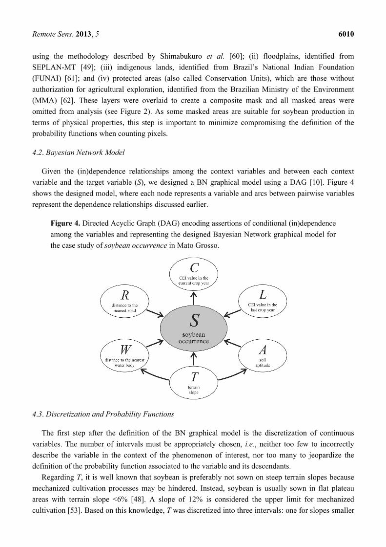
4.2. Bayesian Network Model

Given the (in)dependence relationships among the context variables and between each context

variable and the target variable (S), we designed a BN graphical model using a DAG [10]. Figure 4

shows the designed model, where each node represents a variable and arcs between pairwise variables

represent the dependence relationships discussed earlier.

Figure 4. Directed Acyclic Graph (DAG) encoding assertions of conditional (in)dependence

among the variables and representing the designed Bayesian Network graphical model for

the case study of soybean occurrence in Mato Grosso.

4.3. Discretization and Probability Functions

The first step after the definition of the BN graphical model is the discretization of continuous

variables. The number of intervals must be appropriately chosen, i.e., neither too few to incorrectly

describe the variable in the context of the phenomenon of interest, nor too many to jeopardize the

definition of the probability function associated to the variable and its descendants.

Regarding T, it is well known that soybean is preferably not sown on steep terrain slopes because

mechanized cultivation processes may be hindered. Instead, soybean is usually sown in flat plateau

areas with terrain slope <6% [48]. A slope of 12% is considered the upper limit for mechanized

cultivation [53]. Based on this knowledge, T was discretized into three intervals: one for slopes smaller


than 6%, another for slopes equal to or larger than 6% but smaller than 12%, and the last for slopes

equal to or larger than 12%. As T has no parents, a prior probability function is defined. By pixel

counting, BayNeRD computed the prior probability function for T, considering the defined intervals,

i.e., P(−∞ ≤ T = t < 0.06), P(0.06 ≤ T = t < 0.12), and P(0.12 ≤ T = t < +∞). T is a parent of S, so the

probabilities of soybean occurrence given each defined interval for T were also computed, i.e.,

P(S = s | −∞ ≤ T = t < 0.06), P(S = s | 0.06 ≤ T = t < 0.12), and P(S = s | 0.12 ≤ T = t < +∞). Figure 5

shows a histogram of the discretized T variable and computed probabilities.

Figure 5. Discretization of context variable terrain slope (T) into three intervals. The

percentage at the top of each bar represents the probability of finding a pixel within the

defined interval limits, e.g., P(−∞ ≤ T = t < 0.06) = 82.9%; and the percentage at the

bottom of each bar represents the conditional probability of soybean presence given the

defined interval limits for T, e.g., P(S = 1 | −∞ ≤ T = t < 0.06) = 53.6%.

Figure 5 shows that almost 83% of the analyzed area consists of flat areas, i.e., terrain slope smaller

than 6%. Additionally, it shows that finding soybean plantations in these flat areas (probability of

53.6%) is more likely than in areas where slope is ≥12% (probability of 1.6%).

CEI (C and L) observations are also critical variables for this case study as they are closely related

to soybean occurrence [46]. Figure 6a shows a histogram of L values in the analyzed area with

bimodal appearance. CEI values less than 0.2 are usually associated with targets with low (e.g., forest)

or medium seasonality (e.g., Cerrado or pasture) [63,64]. On the other hand, CEI values greater than

0.2 are strongly associated with high seasonality targets such as annual crops like soybean [65,66].

Based on this knowledge, we empirically defined four intervals for L, as presented in Figure 6b.

Indeed, Figure 6b demonstrates the strong relationship between S and L. Although only 11.6%

(4.6 + 7.0) of Mato Grosso State presented CEI values equal to or greater than 0.2 in the 2004/2005

crop year, the probability of finding soybean plantations in these areas in the 2005/2006 crop year is

considerably greater than in the remaining part of the State.


Figure 6. (a) Histogram of context variable CEI value in the last crop year

(L); (b) Discretization of L into four intervals. The percentage at the top of each bar

represents the probability of finding a pixel within the defined interval limits, e.g.,

P(0.26 ≤ L = l < +∞) = 7.0%; and the percentage at the bottom of each bar represents the

conditional probability of soybean presence given the defined interval limits for L, e.g.,

P(S = 1 | 0.26 ≤ L = l < +∞) = 95.4%.

(a) (b)

Figure 7 shows a histogram of C values with the same bimodal appearance as discussed for L, and a

boxplot, where a strong relationship between soybean presence and C greater than 0.2 is also evident.

Indeed, the relationship between C and S is similar to that between L and S because most soybean

plantations of crop year 2005/2006 were sown over the same areas of crop year 2004/2005 due to the

spatially persistent characteristic of soybean crop over time in Mato Grosso [48]. Thus, for C we used

the same interval limits defined for L.

Figure 7. Histogram of CEI values observed in the current crop year (C) and boxplot

showing the strong relationship between soybean presence (S = 1) and C greater than 0.2.


As with T, L, and C, we manually defined the upper and lower limits for the remaining context

variables, as stated in Table 2. The main advantage of manual definition of interval limits is that it

optimizes experts’ knowledge during the discretization process.

Table 2. Summary of the intervals limits defined for each of the six context variables,

described in Table 1.

Interval # C L A T W R

1 [−∞; 0.05) [−∞; 0.05) low [−∞; 0.06) [−∞; 0.5) [−∞; 3.0)

2 [0.05; 0.20) [0.05; 0.20) high [0.06; 0.12) [0.5; 1.0) [3.0; 8.0)

3 [0.20; 0.26) [0.20; 0.26) [0.12; +∞) [1.0; 2.0) [8.0; +∞)

4 [0.26; +∞) [0.26; +∞) [2.0; +∞)

# of intervals 4 4 2 3 4 3

Intervals are closed on the left and opened on the right, as denoted by [ and ), respectively.

BayNeRD uses the (in)dependence relationships among the variables (Figure 4) and the intervals

defined in the discretization processes (Table 2) to define, based on pixel counting [19], all probability

functions. If a node has no parents (such as L, T, and R) then a prior-probability function is defined;

otherwise, a conditional-probability function that relates the node to its immediate parents is specified

(S, C, A, and W) [10], as shown in Figure 8.

Figure 8. Bayesian network structure and the defined probability function (shown in the

related table) for each variable used in this study case. The six context variables are

described in Table 1 and the interval numbers are detailed in Table 2.

4.4. PI

Based on the designed BN model and the probability functions defined, BayNeRD computes, for

each pixel in the study area, the probability of soybean presence given observations made on the

context variables, i.e.,


( = 1| = , = , = , = , = , = ) (6)

where lower-case letters denote a state or value (defining a particular instantiation) of the respective

discretized variable. The resulting PI was assessed visually and based on official data (i.e., from

IBGE). The PI was also used to generate thematic maps that were statistically assessed, based on the

reference data for testing, to determine the effectiveness of BayNeRD for characterizing

soybean cultivation.

5. Results and Discussion

5.1. Probability Image (PI)

The resulting PI (Figure 9) is an image in which every pixel value represents the calculated

probability as defined in Equation (6).

Figure 9. Probability Image (PI) of soybean presence for the entire Mato Grosso State,

Brazil. Main soybean producer centers and the capital, Cuiabá, are highlighted. The color

indicates the calculated probability of soybean presence in 2005/2006 given the

observations made for the context variables, as expressed by Equation (6).

The PI shows the spatial distribution of (the probability of) soybean crops throughout Mato Grosso

territory in crop year 2005/2006. Green colored pixels represent areas with higher probability of


soybean presence based on observation of the context variables. Some of the main soybean production

centers according to IBGE [67] are highlighted on the PI and allow us to verify the spatial coherence

between PI and official soybean statistics. Previous studies that assessed soybean spatial distribution in

Mato Grosso were also consistent with the regions of higher PI values identified here [42,46].

The higher probabilities shown in Figure 9 highlight traditional centers of soybean production in the

Cerrado biome of Mato Grosso, i.e., Primavera do Leste, Rondonópolis, Sapezal and the central region

(Sorriso Southward). More recent soybean frontiers are in transition regions between Cerrado and the

Amazon biome. In Sorriso municipality Northward (along the BR 163 highway) and Querência region,

which are considered to be the newer agricultural frontiers in Mato Grosso [68], pasturelands have

been converted to soybean plantations [48].

Figure 10 shows, for a small subset of the study area, the set of variables within different conditions

leading to variations in the calculated soybean presence in crop year 2005/2006 (PI). The region

labeled 1 is on a plateau and exhibits ideal conditions for soybean cultivation based on the designed

BN model. CEI values (C and L) are high, predominantly in the upper discretized interval (≥0.26); A is

high; T is flat (<6%); W is ≥2 km; and a road crosses this plateau so R is <3 km. As every context

variable exhibits favorable conditions for soybean presence, the combination of these conditions

results in high probability of soybean presence. The region labeled 2 is on the edge of the plateau and

represents an area where soybean plantations are usually close to pasture lands. In this case three context

variables are favorable for soybean presence based on the criteria discussed above (A, T, and R), but CEI

values (C and L) are unfavorable (≤0.20). Moreover, there are two water bodies in this region further

reducing the probability of soybean plantations. As a result, the probability of soybean presence in

region 2 tended to range between 25% and 50%. The region labeled 3 corresponds to an area of Cerrado,

and exhibits more or less the opposite condition to that of region 1. In this case, all context variables

present unfavorable conditions for soybean presence, leading to probability values close to zero in the PI.

Figure 10. Probability Image (PI) of soybean presence and six context variables (described

in Table 1) zoomed in on the central part of the Sapezal municipality. The legend for the

context variables followed the intervals stated in Table 2. Regions labeled 1, 2, and 3 show

respectively, ideal, intermediate and poor conditions for soybean cultivation.


Various other combinations of context variables can be found in the study area. The BN network is

adept at dealing with such occurrences. According to KL divergence [25], C and L were the most important

variables used to infer about soybean occurrence (KLC = 0.28 and KLL = 0.16, i.e., the KL divergence

for C and L, respectively). It means that, as pointed out by Risso et al. [64], a proper vegetation index

taken at key dates over the crop calendar can be used to identify specific crops such as soybean [69].

In fact, due to its ability and practicability to detect soybean areas, CEI is also used to monitor soybean

plantations in the Brazilian Amazon Biome in the context of the Soy Moratorium [65,66]. For the

remaining context variables A, T, W, and R, the KL divergences were 0.009, 0.002, 0.003, and 0.0001,

respectively. This result means that soil type influenced more the calculated probability of soybean

presence then terrain slope, water distance, and especially the distance to a road.

The relatively small influence of R on the calculated probability of soybean presence could be

explained by the fact that soybean fields are usually very large, particularly in Mato Grosso. Hence,

even very high transportation costs do not hinder soybean cultivation [16]. Additionally, most soybean

areas in Mato Grosso are consolidated (i.e., traditional areas planted with soybean), especially those

surrounding Sapezal, Sorrizo, Rondonópolis, and Primavera do Leste, where transportation logistics

have been developed to fit the available road facilities. However, we expect R to be more influential

close to agricultural frontiers such as in the region of Querência [68]. Indeed, the close relationship

between cash crops’ occurrence and proximity to roads has been widely explored, often using models

to predict future scenarios of agriculture expansion [70] and deforestation [71]. Although modeling

such knowledge is possible in principle using BayNeRD, it was beyond the scope of the present study.

The influence of T on the calculated probability of soybean presence was minimized by the fact that

most parts (83%) of the study were relatively flat (T < 6%—Figure 5). Nevertheless, results showed

that soybean is not likely to be sown in steep areas, corroborating that steep areas are unsuitable for

large scale mechanized agriculture [53,54]. Historically, landholders sow soybean on flat areas, such

as Chapada dos Parecis and those surrounding the BR-163 highway in Mato Grosso central

(e.g., Sorriso region), where the large soybean hubs are located [58].

In general, where only one context variable is unfavorable and/or is not strongly related to soybean

occurrence (such as W, which presented KLW = 0.003), any decrease in the calculated probability of

soybean presence is likely to be very small. However if the context variable has a strong relationship

with soybean occurrence (for example C, which presented KLC = 0.28), any unfavorable condition of

this variable is likely to decrease soybean probability values substantially. Additionally, the mixing

within a pixel size of 250 × 250 m (defined as our nominal spatial resolution), especially over the

boundaries of defined discretized intervals, could be noted in Figure 10, which presented both orange

and light-green colored pixels surrounding green pixels in the PI.

5.2. Creating Thematic Maps from the PI

The PI, as shown in Figure 9, is the main output of BayNeRD and may be used in a range of different

applications. For example, if one is looking for soybean areas for environmental supervision of soybean

plantations in recent deforested areas, as defined in the Soy Moratorium context in Brazil [65,66], then

areas where the probability of presence of soybean is high could be prioritized and the PI could be

used to guide the logistics of field inspection by regulatory agencies [19]. The PI can also be used as


input for classifiers (e.g., as prior probability for the maximum likelihood classifier) or to mask out

low probability areas before running a classification.

Additionally, the PI can also be used to produce a thematic map (e.g., for acreage estimates) by

applying a threshold probability value where all pixels with values above the threshold are allocated to

the target thematic class (e.g., soybean). This value, herein called TPV, can be defined as any real

value between 0% and 100%. Apart from a manually defined TPV, six criteria were implemented in

BayNeRD to select a TPV according to some criterion, as defined in Section 3.6. Selecting the TPV,

using reference information (e.g., reference data for testing). The TPV that produces the most suitable

thematic map, following the chosen criterion, is then called the best TPV.

The goal is to find the TPV that generates the most suitable thematic map showing two classes:

target (soybean) and non-target (non-soybean). Several metrics are discussed in the literature to access

map accuracy [72,73]. The most widely used one is the kappa index [28,74]. However, in the case of

binary classifications, Foody [75] pointed out the advantages of two complimentary indices: sensitivity

and specificity [27]. These indices indicate the ability to find true positives (e.g., soybean areas which

are correctly labeled soybean) and true negatives (e.g., non-soybean areas, which are correctly labeled

non-soybean), respectively.

By varying the TPV from 0% to 100% different thematic maps were produced. Obviously, TPV = 0%

produced a thematic map where all pixels within the study area were labeled as soybean. When all

pixels were labeled soybean, all true soybean areas were then labeled as soybean and consequently

sensitivity was equal to 100%. On the other hand, all true non-soybean areas were also labeled as

soybean, and, consequently, specificity was 0%. With TPV increasing from 0 to 100%, sensitivity

decreases while specificity increases. A useful graph to represent accuracy assessment in terms of these

two indices is known as a Receiver Operating Characteristic (ROC) curve [76]. In an ROC curve the

sensitivity is plotted on the Y-axis while the X-axis represents 1-specificity. Thus, the upper left corner

represents the ideal point of 100% sensitivity and 100% specificity. According to Zweig & Campbell [26],

the closer the point is to the upper left corner in a ROC curve, the higher the overall accuracy of the

thematic map. Therefore, the used nearest 100% sensitivity and 100% specificity point criterion aimed

at selecting the TPV that produces a thematic map where its corresponding point in a ROC curve is

closest to the upper left corner, based on the reference data for testing. Figure 11 shows a ROC curve

produced by varying TPV from 0% to 100%.

In the ROC curve presented in Figure 11 all points plotted above the diagonal (random guess)

represent a strong classification result (i.e., better than random) [76]. This indicates that the PI is an

accurate representation of the phenomenon (in this case, soybean occurrence). According to the

nearest 100% sensitivity and 100% specificity point criterion, the best TPV should be 47%, resulting in

a thematic map with sensitivity of 90.0% and specificity of 92.2%.Moreover, the overall accuracy of

91.1% and a kappa value of 0.82 corroborated the fact that this best TPV produced an accurate

thematic map of soybean areas, based on the reference data for testing. Figure 12 shows the accuracy

indices for the PI-derived thematic maps generated by varying TPV from 0% to 100%.


Figure 11. Receiver Operating Characteristic (ROC) curve, depicting sensitivity and

specificity indices associated with thematic maps generated from the Probability Image

(PI) by varying the Target Probability Value (TPV) from 0% to 100%. The circle points

out the best TPV according to the chosen criterion.

Figure 12. Accuracy indices associated with thematic maps generated from the Probability

Image (PI) by varying the Target Probability Value (TPV) from 0% to 100%. The vertical

line identifies the best TPV, according to the chosen criterion, highlighting the accuracy

achieved according to each index (described in the legend).


A TPV can be defined to be more or less restricted in terms of associating a degree of belief,

represented by a probability value, in which a pixel can be associated to the target thematic class,

prioritizing either sensitivity or specificity. If the aim is that the total soybean area of the final thematic

map closely matches the official statistics, the TPV can also be selected accordingly. For example, the

thematic map generated with a TPV (manually defined) equal to 84% is more restrictive in terms of

labeling a pixel as soybean but best matched the official soybean acreage for the 2005/2006 crop year

in Mato Grosso. Indeed this thematic map presented 6.1 Mha of soybean—only 0.8% higher than the

official data published by IBGE [67].

Similar to mapping soybean using remote sensing and environmental variables, Krug et al. [77]

used various environmental observations such as sea surface temperature and wind velocity in BNs to

investigate coral bleaching along the Bahia State coast, Brazil. They also pointed out that BNs could

be used as a prediction tool, incorporating evidence from a large data set of environmental observations,

as we demonstrated here. In fact, BayNeRD could be used to infer knowledge about a variety of

phenomena based on observations of variables that are somehow related to the phenomena. For example,

it may be used to identify forested areas susceptible to burning based on observations of forcing variables

such as selective logging, deforestation, rainfall, distance to roads, and land use type of surrounding

areas [78,79]. Detecting landslide susceptibility based on observations made upon variables such as

slope, soil, lithological classes, terrain curvature, land cover, and rainfall represents another possible

application of BayNeRD [80]. BayNERD could also enable inference about the occurrence of

certain fish species based on data such as sea surface temperature, chlorophyll concentration and sea

surface winds [81].

6. Conclusion

This paper described the basis functioning and implementation of a computer aided BN method for

raster data analysis: Bayesian Networks for Raster Data (BayNeRD). BayNeRD provides a new

computer-aided method to characterize phenomena through plausible reasoning inferences based on

observations of several variables. The number of variables is not limited and the sole conditions are an

accurate match of raster cells and the availability of a suitable reference data set.

The case study of mapping soybean areas in Mato Grosso State, Brazil, showed BayNeRD’s capability

to model environmental phenomena. Based on observations made upon Crop Enhanced Index (CEI)

values for the current and last crop years, soil type, terrain slope, and distance to the nearest road and

water body, the resulting Probability Image (PI) from BayNeRD depicted a spatial distribution of

soybean areas consistent with expert knowledge and official statistical data. Furthermore, the PI was

used to produce soybean thematic maps by varying the Target Probability Value (TPV) according to

different criteria, achieving an overall accuracy greater than 91% or a soybean acreage estimation with

more than 99% in accordance with the official data.

Advantages of BayNeRD include that it incorporates expert’s knowledge into the process; it models

the (in)dependence relationships among several observed variables; it outputs variable importance

information, through the Kullback-Leibler divergence; it can accommodate different forms of data

(numerical and categorical); it can handle incomplete data; it allows computation of probability


functions from the data; and it is a user-friendly implementation in a free software ready to handle

raster data sets.

The BayNeRD algorithm has been implemented in R software [20] and can be found on the

internet. As future work, we plan to add some improvements in the BayNeRD algorithm, such as:

automating both the discretization process as well as the definition of (in)dependence relationships

among variables [82]; possibility to define more than two classes for the target variable; and explicit

spatial influence, such as neighborhood structures [83].

Acknowledgments

The authors thank Nikolay Balov, from the University of Rochester Medical Center, for assistance

with the catnet R package; Ruy Dalla Valle Epiphanio for sharing part of the dataset used in this work;

the Brazilian Research Councils CNPq (Conselho Nacional do Desenvolvimento Científico e

Tecnológico—142845/2011-6 and 158877/2013-6), CAPES (Coordenação de Aperfeiçoamento de

Pessoal de Nível Superior—33010013005P0) and Fapesp (Fundação de Amparo à Pesquisa do Estado

de São Paulo—2008/56252-0), and the German Exchange Service DAAD (Deutscher Akademischer

Austausch Dienst—12/A/72898) for financial support; and the anonymous referees for their

constructive comments and suggestions.

Conflicts of Interest

The authors declare no conflict of interest.

References

1. Melesse, A.M.; Weng, Q.; Thenkabail, P.S.; Senay, G.B. Remote sensing sensors and applications

in environmental resources mapping and modelling. Sensors 2007, 7, 3209–3241.

2. Donner, R.; Barbosa, S.; Kurths, J.; Marwan, N. Understanding the earth as a complex

system—Recent advances in data analysis and modelling in Earth sciences. Eur. Phys. J. Spec.

Top. 2009, 174, 1–9.

3. Li, Z., Chen, J., Baltsavias, E., Eds. Advances in Photogrammetry, Remote Sensing and Spatial

Information Sciences: 2008 ISPRS Congress Book, 1st ed.; CRC Press: Trowbridge, UK, 2008;

Volume 23, p. 546.

4. Lee, C.A.; Gasster, S.D.; Plaza, A.; Chang, C.-I.; Huang, B. Recent developments in high

performance computing for remote sensing: A review. IEEE J. Sel. Top. Appl. Earth Obs. Remote

Sens. 2011, 4, 508–527.

5. Lu, D.; Weng, Q. A survey of image classification methods and techniques for improving

classification performance. Int. J. Remote Sens. 2007, 28, 823–870.

6. Richards, J.A. Analysis of remotely sensed data: The formative decades and the future.

IEEE Trans. Geosci. Remote Sens. 2005, 43, 422–432.

7. Jaynes, E.T. Probability Theory: The Logic of Science; Cambridge University Press: Cambridge,

UK, 2003; p. 727.


8. McGrayne, S.B. The Theory that would not Die: How Bayes’ Rule Cracked the Enigma Code,

Hunted down Russian Submarines, and Emerged Triumphant from Two Centuries of Controversy;

Yale University Press: New Haven, CT, USA, 2011; p. 336.

9. Pearl, J. Probabilistic Reasoning in Intelligent Systems: Networks of Plausible Inference, 1st ed.;

Morgan Kaufmann: San Francisco, CA, USA, 1988; p. 552.

10. Jensen, F.V.; Nielsen, T.D. Bayesian Networks and Decision Graphs, 2nd ed.; Springer:

New York, NY, USA, 2007; p. 447.

11. Neapolitan, R.E. Learning Bayesian Networks; Prentice Hall: Upper Saddle River, NJ, USA,

2003; p. 674.

12. Darwiche, A. Modeling and Reasoning with Bayesian Networks; Cambridge University Press:


13. Heckerman, D. Bayesian networks for data mining. Data Min. Knowl. Discov. 1997, 1, 79–119.

14. Uusitalo, L. Advantages and challenges of Bayesian networks in environmental modelling.

Ecol. Model. 2007, 203, 312–318.

15. Aguilera, P.A.; Fernández, A.; Fernández, R.; Rumí, R.; Salmerón, A. Bayesian networks in

environmental modelling. Environ. Model. Softw. 2011, 26, 1376–1388.

16. Garrett, R.D.; Lambin, E.F.; Naylor, R.L. Land institutions and supply chain configurations as

determinants of soybean planted area and yields in Brazil. Land Use Policy 2013, 31, 385–396.

17. Park, S.; McSweeney, K.; Lowery, B. Identification of the spatial distribution of soils using a

process-based terrain characterization. Geoderma 2001, 103, 249–272.

18. Cooper, G.F.; Herskovits, E. A Bayesian method for the induction of probabilistic networks from

data. Mach. Learn. 1992, 9, 309–347.

19. Mello, M.P.; Rudorff, B.F.T.; Adami, M.; Rizzi, R.; Aguiar, D.A.; Gusso, A.; Fonseca, L.M.G.

A Simplified Bayesian Network to Map Soybean Plantations. In Proceedings of 2010 IEEE

International Geoscience and Remote Sensing Symposium, Honolulu, HI, USA, 25–30 July 2010;

pp. 351–354.

20. R Core Team. R: A Language and Environment for Statistical Computing; R Foundation for

Statistical Computing: Vienna, Austria, 2013.

21. Crawley, M.J. The R Book; John Wiley & Sons: Chichester, UK, 2007; p. 950.

22. Bivand, R.S.; Pebesma, E.J.; Gómez-Rubio, V. Applied Spatial Data Analysis with R; Springer:


23. Albert, J. Bayesian Computation with R, 2nd ed.; Springer: New York, NY, USA, 2009; p. 298.

24. Balov, N.; Salzman, P. catnet: Categorical Bayesian Network Inference. R Package Version 1.14.2.

Available online: http://CRAN.R-project.org/package=catnet (accessed on 18 August 2013).

25. Kullback, S.; Leibler, R.A. On information and sufficiency. Ann. Math. Stat. 1951, 22, 79–86.

26. Zweig, M.H.; Campbell, G. Receiver-operating characteristic (ROC) plots: A fundamental evaluation

tool in clinical medicine. Clin. Chem. 1993, 39, 561–577.

27. Altman, D.G.; Bland, J.M. Statistics notes: Diagnostic tests 1: Sensitivity and specificity. BMJ

1994, 308, 1552–1552.

28. Cohen, J. A coefficient of agreement for nominal scales. Educ. Psychol. Measur. 1960, 20, 37–46.

29. Hudson, W.D. Correct formulation of the Kappa coefficient of agreement. Photogramm. Eng.

Remote Sens. 1987, 53, 421–422.


30. Congalton, R.G.; Green, K. Assessing the Accuracy of Remotely Sensed Data: Principles and

Pratices, 2nd ed.; CRC Press: Boca Raton, FL, USA, 2009; p. 183.

31. CONAB. Séries Históricas Relativas às Safras 1976/77 a 2011/2012 de Área Plantada,

Produtividade e Produção. Available online: http://www.conab.gov.br/conteudos.php?a=1252&t=

(accessed on 21 March 2013).

32. BRASIL. Resolução da Presidência do IBGE de n° 5 (R.PR-5/02) de 10 de outubro de 2002;

Diário Oficial da União: Brasília, DF, Brazil, 2002; pp. 48–69.

33. Epiphanio, R.D.V.; Formaggio, A.R.; Rudorff, B.F.T.; Maeda, E.E.; Luiz, A.J.B. Estimating

soybean crop areas using spectral-temporal surfaces derived from MODIS images in Mato

Grosso, Brazil. Pesquisa Agropecuária Brasileira 2010, 45, 72–80.

34. FAO. FAOSTAT: FAO Statistical Database. Available online: http://faostat.fao.org (accessed on

9 April 2012).

35. Atzberger, C. Advances in remote sensing of agriculture: Context description, existing operational

monitoring systems and major information needs. Remote Sens. 2013, 5, 949–981.

36. Rudorff, B.F.T.; Aguiar, D.A.; Silva, W.F.; Sugawara, L.M.; Adami, M.; Moreira, M.A. Studies

on the rapid expansion of sugarcane for ethanol production in São Paulo State (Brazil) using

Landsat data. Remote Sens. 2010, 2, 1057–1076.

37. Rizzi, R.; Rudorff, B.F.T. Estimativa da área de soja no Rio Grande do Sul por meio de imagens

Landsat. Revista Brasileira de Cartografia 2005, 57, 226–234.

38. Vieira, M.A.; Formaggio, A.R.; Rennó, C.D.; Atzberger, C.; Aguiar, D.A.; Mello, M.P. Object

based image analysis and data mining applied to a remotely sensed Landsat time-series to map

sugarcane over large areas. Remote Sens. Environ. 2012, 123, 553–562.

39. Mello, M.P.; Vieira, C.A.O.; Rudorff, B.F.T.; Aplin, P.; Santos, R.D.C.; Aguiar, D.A. STARS:

A new method for multitemporal remote sensing. IEEE Trans. Geosci. Remote Sens. 2013, 51,

1897–1913.

40. Asner, G.P. Cloud cover in Landsat observations of the Brazilian Amazon. Int. J. Remote Sens.

2001, 22, 3855–3862.

41. Sano, E.E.; Ferreira, L.G.; Asner, G.P.; Steinke, E.T. Spatial and temporal probabilities of

obtaining cloud-free Landsat images over the Brazilian tropical savanna. Int. J. Remote Sens.

2007, 28, 2739–2752.

42. Arvor, D.; Jonathan, M.; Meirelles, M.S.P.; Dubreuil, V.; Durieux, L. Classification of MODIS

EVI time series for crop mapping in the state of Mato Grosso, Brazil. Int. J. Remote Sens. 2011,

32, 7847–7871.

43. Macedo, M.N.; DeFries, R.S.; Morton, D.C.; Stickler, C.M.; Galford, G.L.; Shimabukuro, Y.E.

Decoupling of deforestation and soy production in the southern Amazon during the late 2000s.

Proc. Natl. Acad. Sci. USA 2012, 109, 1341–1346.

44. Morton, D.C.; DeFries, R.S.; Shimabukuro, Y.E.; Anderson, L.O.; Arai, E.; del Bon Espirito-Santo, F.;

Freitas, R.M.; Morisette, J. Cropland expansion changes deforestation dynamics in the southern

Brazilian Amazon. Proc. Natl. Acad. Sci. USA 2006, 103, 14637–14641.

45. Justice, C.; Townshend, J.R.G.; Vermote, E.; Masuoka, E.; Wolfe, R.; Saleous, N.; Roy, D.;

Morisette, J. An overview of MODIS land data processing and product status. Remote Sens.

Environ. 2002, 83, 3–15.


46. Rizzi, R.; Risso, J.; Epiphanio, R.D.V.; Rudorff, B.F.T.; Formaggio, A.R.; Shimabukuro, Y.E.;

Fernandes, S.L. Estimativa da área de Soja no Mato Grosso por meio de Imagens MODIS.

In Proceedings of the 14th Brazilian Remote Sensing Symposium, Natal, RN, Brazil, 25–30 April

2009; INPE: São José dos Campos, SP, Brazil, 2009; pp. 387–394.

47. Huete, A.R.; Didan, K.; Miura, T.; Rodriguez, E.; Gao, X.; Ferreira, L.G. Overview of the

radiometric and biophysical performance of the MODIS vegetation indices. Remote Sens.

Environ. 2002, 83, 195–213.

48. Risso, J. Diagnóstico Espacialmente Explícito da Expansão da Soja no Mato Grosso de 2000 a

2012; National Institute for Space Research: São José dos Campos, SP, Brazil, 2013; p. 110.

49. SEPLAN-MT. Sistema Interoperável de Informações Geoespaciais do Estado do Mato Grosso

(SIIGEO). Available online: http://www.siigeo.mt.gov.br/ (accessed on 14 April 2012).

50. Palmiere, F.; Santos, H.G.; Gomes, I.A.; Lumbreras, J.F.; Aglio, M.M.D. The Brazilian Soil

Classification System. In Soil Classification: A Global Desk Reference; Rice, T., Eswaran, H.,

Stewart, B., Ahrens, R., Eds.; CRC Press: Boca Raton, FL, USA, 2002; pp. 127–146.

51. Sistema Brasileiro de Classificação de Solos, 2nd ed.; Santos, H.G., Oliveira, J.B., Lumbrelas, J.F.,

Anjos, L.H.C., Coelho, M.R., Jacomine, P.K.T., Cunha, T.J.F., Oliveira, V.Á., Eds.;

Embrapa Solos: Rio de Janeiro, RJ, Brazil, 2006; p. 306.

52. Rabus, B.; Eineder, M.; Roth, A.; Bamler, R. The shuttle radar topography mission—A new class

of digital elevation models acquired by spaceborne radar. ISPRS J. Photogramm. Remote Sens.

2003, 57, 241–262.

53. Shaxson, F. New Concepts and Approaches to Land Management in the Tropics with Emphasis

on Steeplands; FAO: Rome, Italy, 1999; p. 125.

54. Seeruttun, S.; Crossley, C.P. Use of digital terrain modelling for farm planning for mechanical

harvest of sugar cane in Mauritius. Comput. Electron. Agric. 1997, 18, 29–42.

55. ANEEL. Sistema de Informações Georeferenciadas do Setor Elétrico (SIGEO). Available online:

http://sigel.aneel.gov.br (accessed on 20 April 2012).

56. Silva, J.A.A.; Nobre, A.D.; Joly, C.A.; Nobre, C.A.; Manzatto, C.V.; Rech Filho, E.L.; Skorupa, L.A.;

May, P.H.; Cunha, M.M.L.C.; Rodrigues, R.R.; et al. Brazil Forest Code and Science: Contributions

to the Dialogue, 2nd ed.; The Brazilian Society for the Advancement of Science—SBPC:

São Paulo, SP, Brazil, 2012; p. 147.

57. IBGE. Maps. Available online: http://mapas.ibge.gov.br/en/ (accessed on 29 April 2012).

58. Fearnside, P.M. Soybean cultivation as a threat to the environment in Brazil. Environ. Conserv.

2002, 28, 23–38.

59. INPE. PRODES: Projeto de Monitoramento do Desflorestamento na Amazônia Legal. Available

online: http://www.obt.inpe.br/prodes/index.php (accessed on 20 January 2012).

60. Shimabukuro, Y.E.; Batista, G.T.; Mello, E.M.K.; Moreira, J.C.; Duarte, V. Using shade fraction

image segmentation to evaluate deforestation in Landsat Thematic Mapper images of the Amazon

Region. Int. J. Remote Sens. 1998, 19, 535–541.

61. FUNAI. Maps. Available online: http://mapas.funai.gov.br (accessed on 20 January 2013).

62. MMA. Download de Dados Geográficos. Available online: http://mapas.mma.gov.br/i3geo/

datadownload.htm (accessed on 20 January 2013).


63. Galford, G.L.; Mustard, J.F.; Melillo, J.; Gendrin, A.; Cerri, C.C.; Cerri, C.E. Wavelet analysis of

MODIS time series to detect expansion and intensification of row-crop agriculture in Brazil.

Remote Sens. Environ. 2008, 112, 576–587.

64. Risso, J.; Rizzi, R.; Rudorff, B.F.T.; Adami, M.; Shimabukuro, Y.E.; Formaggio, A.R.;

Epiphanio, R.D.V. Índices de vegetação Modis aplicados na discriminação de áreas de soja.

Pesquisa Agropecuária Brasileira 2012, 47, 1317–1326.

65. Rudorff, B.F.T.; Adami, M.; Risso, J.; de Aguiar, D.A.; Pires, B.; Amaral, D.; Fabiani, L.;

Cecarelli, I. Remote sensing images to detect soy plantations in the amazon biome—The soy

moratorium initiative. Sustainability 2012, 4, 1074–1088.

66. Rudorff, B.F.T.; Adami, M.; Aguiar, D.A.; Moreira, M.A.; Mello, M.P.; Fabiani, L.; Amaral, D.F.;

Pires, B.M. The soy moratorium in the Amazon biome monitored by remote sensing images.

Remote Sens. 2011, 3, 185–202.

67. IBGE. Sistema IBGE de Recuperação Automática (SIDRA)—Produção Agrícola Municipal

(PAM) 2012. Avaiable online: http://www.sidra.ibge.gov.br (accessed on 2 July 2012).

68. Jepson, W. Producing a modern agricultural frontier: Firms and cooperatives in Eastern Mato

Grosso, Brazil. Econ. Geogr. 2009, 82, 289–316.

69. Rizzi, R.; Rudorff, B.F.T.; Shimabukuro, Y.E.; Doraiswamy, P.C. Assessment of MODIS LAI

retrievals over soybean crop in Southern Brazil. Int. J. Remote Sens. 2006, 27, 4091–4100.

70. Jasinski, E.; Morton, D.; DeFries, R.; Shimabukuro, Y.; Anderson, L.; Hansen, M. Physical

landscape correlates of the expansion of mechanized agriculture in Mato Grosso, Brazil.

Earth Interact. 2005, 9, 1–18.

71. Soares-Filho, B.S.; Nepstad, D.C.; Curran, L.M.; Cerqueira, G.C.; Garcia, R.A.; Ramos, C.A.;

Voll, E.; McDonald, A.; Lefebvre, P.; Schlesinger, P. Modelling conservation in the Amazon

basin. Nature 2006, 440, 520–523.

72. Foody, G.M. Status of land cover classification accuracy assessment. Remote Sens. Environ.

2002, 80, 185–201.

73. Liu, C.; Frazier, P.; Kumar, L. Comparative assessment of the measures of thematic classification

accuracy. Remote Sens. Environ. 2007, 107, 606–616.

74. Smits, P.C.; Dellepiane, S.G.; Schowengerdt, R.A. Quality assessment of image classification

algorithms for land-cover mapping: A review and a proposal for a cost-based approach. Int. J.

Remote Sens. 1999, 20, 1461–1486.

75. Foody, G.M. Assessing the accuracy of land cover change with imperfect ground reference data.

Remote Sens. Environ. 2010, 114, 2271–2285.

76. Hanley, J.A.; McNeil, B.J. The meaning and use of the area under a receiver operating

characteristic (ROC) curve. Radiology 1982, 143, 29–36.

77. Krug, L.A.; Gherardi, D.F.M.; Stech, J.L.; Leão, Z.M.A.N.; Kikuchi, R.K.P.; Hruschka, E.R.;

Suggett, D.J. The construction of causal networks to estimate coral bleaching intensity.

Environ. Model. Softw. 2013, 42, 157–167.

78. Silvestrini, R.A.; Soares-Filho, B.S.; Nepstad, D.; Coe, M.; Rodrigues, H.; Assunção, R.

Simulating fire regimes in the Amazon in response to climate change and deforestation.

Ecol. Appl. Public. Ecol. Soc. Am. 2011, 21, 1573–1590.


79. Aragão, L.E.O.C.; Malhi, Y.; Barbier, N.; Lima, A.; Shimabukuro, Y.; Anderson, L.; Saatchi, S.

Interactions between rainfall, deforestation and fires during recent years in the Brazilian

Amazonia. Philos. Trans. R. Soc. Lond. Ser. B Biol. Sci. 2008, 363, 1779–1785.

80. Fell, R.; Corominas, J.; Bonnard, C.; Cascini, L.; Leroi, E.; Savage, W.Z. Guidelines for landslide

susceptibility, hazard and risk zoning for land-use planning. Eng. Geol. 2008, 102, 99–111.

81. Oliveira, F.S.C.; Gherardi, D.F.M.; Stech, J.L. The relationship between multi-sensor satellite

data and Bayesian estimates for skipjack tuna catches in the South Brazil Bight. Int. J. Remote

Sens. 2010, 31, 4049–4067.

82. Li, L.; Wang, J.; Leung, H.; Jiang, C. Assessment of catastrophic risk using Bayesian network

constructed from domain knowledge and spatial data. Risk Anal. 2010, 30, 1157–1175.

83. Rodrigues, E.C.; Assunção, R. Bayesian spatial models with a mixture neighborhood structure.

J. Multivar. Anal. 2012, 109, 88–102.

© 2013 by the authors; licensee MDPI, Basel, Switzerland. This article is an open access article

distributed under the terms and conditions of the Creative Commons Attribution license

(http://creativecommons.org/licenses/by/3.0/).

Date post:	04-Feb-2022
Category:	Documents
Upload:	others
View:	2 times
Download:	0 times

Bayesian Networks for Raster Data (BayNeRD): Plausible

Documents