86
2016-03-17 Byoung-Hee Kim, Seong-Ho Son Biointelligence Lab, CSE, Seoul National University Bayesian Networks Practice Part 2
2016-03-17
Byoung-Hee Kim, Seong-Ho Son
Biointelligence Lab, CSE,
Seoul National University
Bayesian Networks Practice
Part 2
Agenda
Probabilistic Inference in Bayesian networks
Probability basics
D-separation
Probabilistic inference in polytrees
Exercise
Inference by hand (self)
Inference by GeNIe (self)
Learning from data using Weka
Appendix
AI & Uncertainty
© 2014-2016, SNU CSE Biointelligence Lab., http://bi.snu.ac.kr 2
© 2014-2016, SNU CSE Biointelligence Lab., http://bi.snu.ac.kr 3
(DAG)

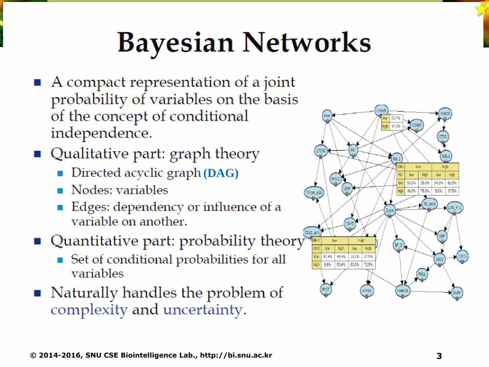
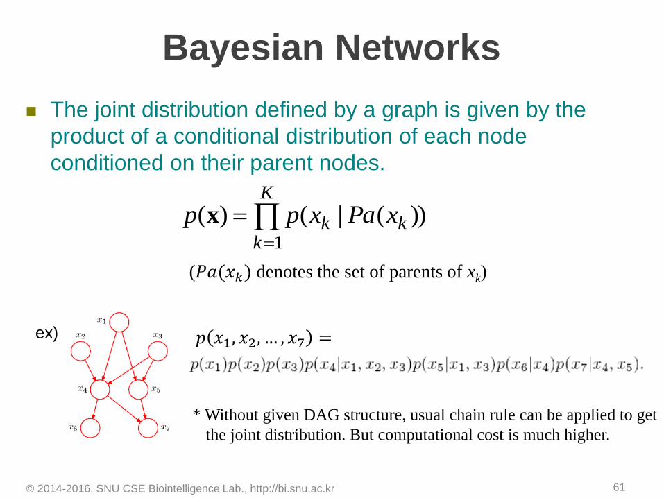
Bayesian Networks
The joint distribution defined by a graph is given by the product of a conditional distribution of each node conditioned on their parent nodes.
© 2014-2016, SNU CSE Biointelligence Lab., http://bi.snu.ac.kr 4
𝑝 𝑥1, 𝑥2, … , 𝑥7 =
(𝑃𝑎(𝑥𝑘) denotes the set of parents of xk)
K
kkk xPaxpp
1
))(|()(x
ex)
* Without given DAG structure, usual chain rule can be applied to get
the joint distribution. But computational cost is much higher.

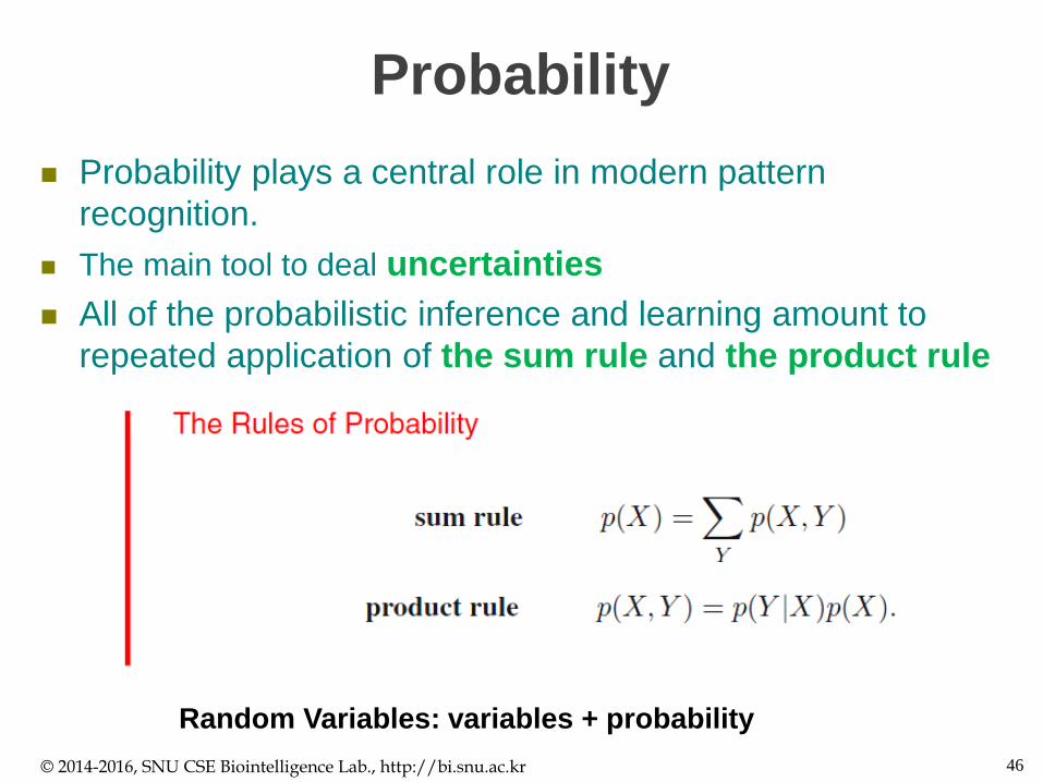
Probability
Probability plays a central role in modern pattern recognition.
The main tool to deal uncertainties
All of the probabilistic inference and learning amount to repeated application of the sum rule and the product rule
© 2014-2016, SNU CSE Biointelligence Lab., http://bi.snu.ac.kr 5
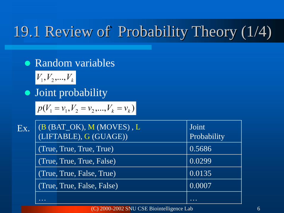
Random Variables: variables + probability
(C) 2000-2002 SNU CSE Biointelligence Lab 6
19.1 Review of Probability Theory (1/4)
Random variables
Joint probability
(B (BAT_OK), M (MOVES) , L
(LIFTABLE), G (GUAGE))
Joint
Probability
(True, True, True, True) 0.5686
(True, True, True, False) 0.0299
(True, True, False, True) 0.0135
(True, True, False, False) 0.0007
… …
Ex.
(C) 2000-2002 SNU CSE Biointelligence Lab 7
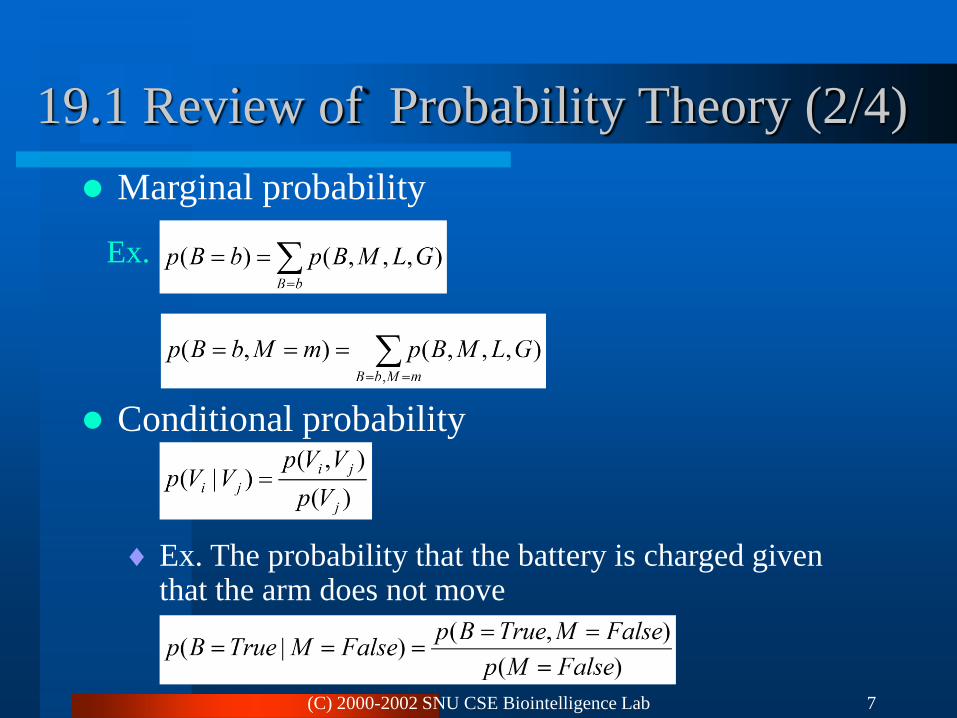
19.1 Review of Probability Theory (2/4)
Marginal probability
Conditional probability
Ex. The probability that the battery is charged given that the arm does not move
Ex.
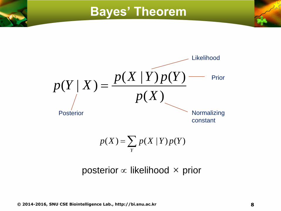
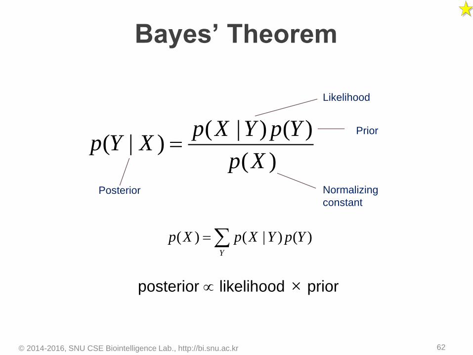
Bayes’ Theorem
© 2014-2016, SNU CSE Biointelligence Lab., http://bi.snu.ac.kr 8
( | ) ( )( | )
( )
p X Y p Yp Y X
p X
( ) ( | ) ( )Y
p X p X Y p Y
Posterior
Likelihood
Prior
Normalizing
constant
posterior likelihood × prior
Bayes’ Theorem
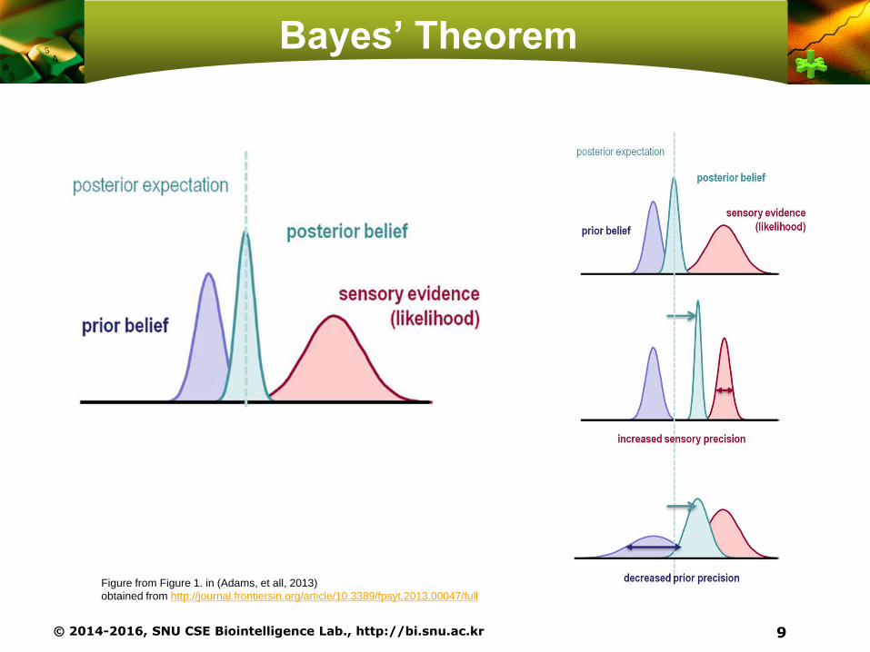
© 2014-2016, SNU CSE Biointelligence Lab., http://bi.snu.ac.kr 9
Figure from Figure 1. in (Adams, et all, 2013)
obtained from http://journal.frontiersin.org/article/10.3389/fpsyt.2013.00047/full

Bayesian Probabilities-Frequentist vs. Bayesian
Likelihood: Frequentist
w: a fixed parameter determined by ‘estimator’ Maximum likelihood: Error function = Error bars: Obtained by the distribution of possible data sets
Bootstrap
Cross-validation
Bayesian a probability distribution w: the uncertainty in the
parameters Prior knowledge
Noninformative (uniform) prior, Laplace correction in estimating priors
Monte Carlo methods, variational Bayes, EP
© 2014-2016, SNU CSE Biointelligence Lab., http://bi.snu.ac.kr 10
( | ) ( )( | )
( )
p pp
p
w ww
DD
D
( | )p wD
log ( | )p wDD
Thomas Bayes
(See an article ‘WHERE Do PROBABILITIES COME FROM?’ on page 491 in the textbook (Russell and Norvig, 2010) for more discussion)

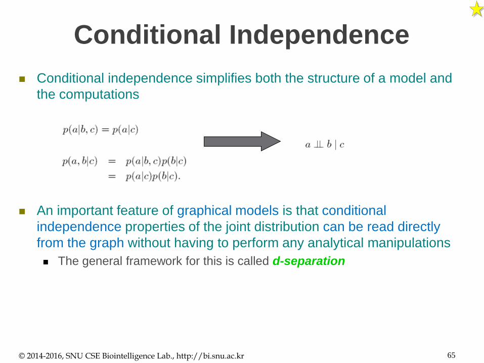
Conditional Independence
Conditional independence simplifies both the structure of a model and the computations
An important feature of graphical models is that conditional independence properties of the joint distribution can be read directly from the graphwithout having to perform any analytical manipulations
The general framework for this is called d-separation
© 2014-2016, SNU CSE Biointelligence Lab., http://bi.snu.ac.kr 11
(C) 2000-2002 SNU CSE Biointelligence Lab 12
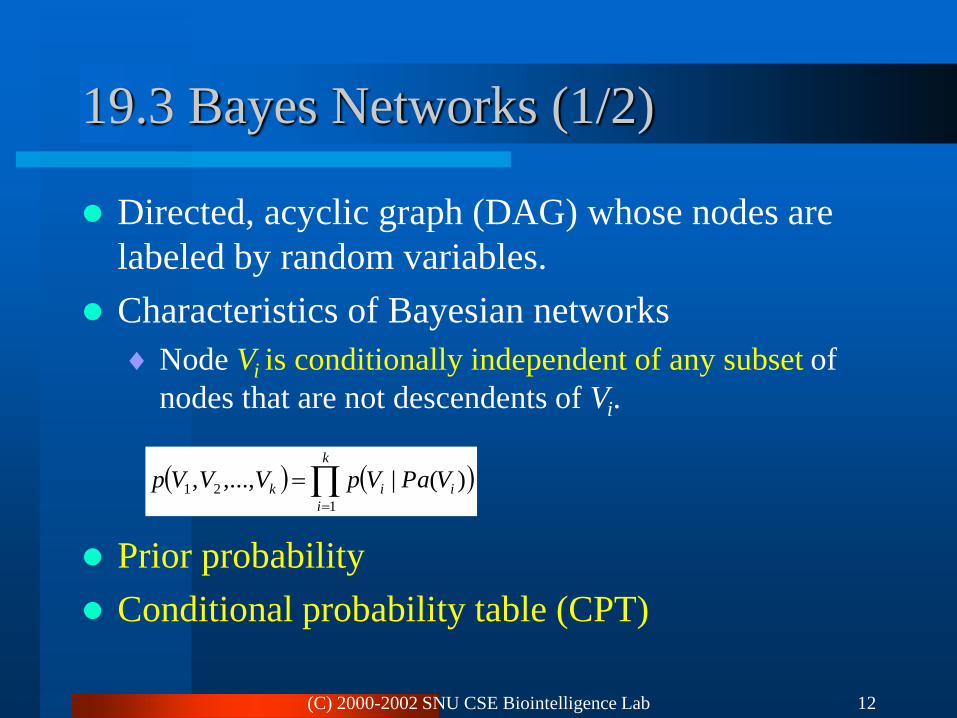
19.3 Bayes Networks (1/2)
Directed, acyclic graph (DAG) whose nodes are
labeled by random variables.
Characteristics of Bayesian networks
Node Vi is conditionally independent of any subset of
nodes that are not descendents of Vi.
Prior probability
Conditional probability table (CPT)
k
i
iik VPaVpVVVp1
21 )(|,...,,
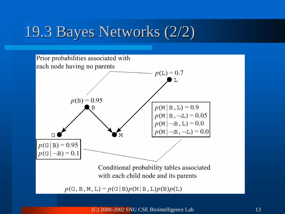
(C) 2000-2002 SNU CSE Biointelligence Lab 13
19.3 Bayes Networks (2/2)

(C) 2000-2002 SNU CSE Biointelligence Lab 14
19.4 Patterns of Inference in Bayes
Networks (1/3)
Causal or top-down inference
Ex. The probability that the arm moves given that the block is
liftable
BpLBMpBpLBMp
LBpLBMpLBpLBMp
LBMpLBMpLMp
,|,|
|,||,|
|,|,|
(C) 2000-2002 SNU CSE Biointelligence Lab 15
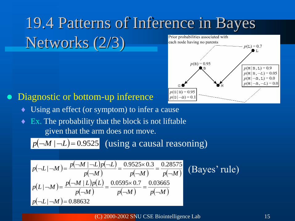
19.4 Patterns of Inference in Bayes
Networks (2/3)
Diagnostic or bottom-up inference
Using an effect (or symptom) to infer a cause
Ex. The probability that the block is not liftable
given that the arm does not move.
9525.0| LMp (using a causal reasoning)
88632.0|
03665.07.00595.0||
28575.03.09525.0||
MLp
MpMpMp
LpLMpMLp
MpMpMp
LpLMpMLp (Bayes’ rule)
(C) 2000-2002 SNU CSE Biointelligence Lab 16
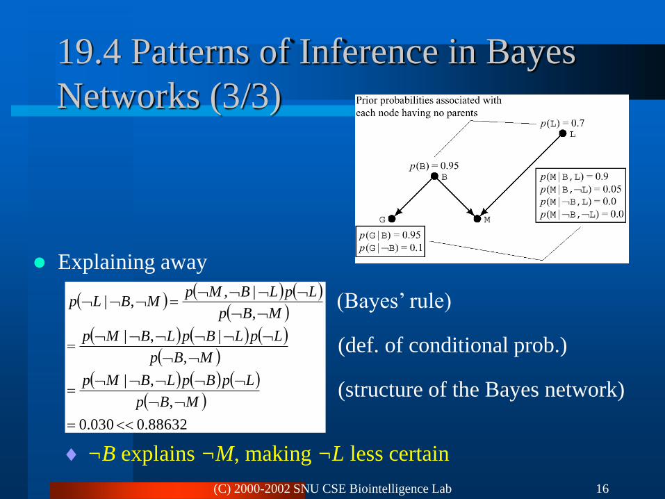
19.4 Patterns of Inference in Bayes
Networks (3/3)
Explaining away
¬ B explains ¬ M, making ¬ L less certain
88632.0030.0
,
,|
,
|,|
,
|,,|
MBp
LpBpLBMp
MBp
LpLBpLBMp
MBp
LpLBMpMBLp (Bayes’ rule)
(def. of conditional prob.)
(structure of the Bayes network)

Ex1 : c is tail-to-tail node
because both arcs on the
path lead out of c.
Ex2 : c is head-to-tail node
because one arc on the path
leads in to c, while the other
leads out.
d-separation
Tail-to-tail node or head-to-tail node
Think of ‘head’ as parent node and ‘tail’ as descendant node.
The path is blocked if the node is observed.
The path is unblocked if the node is unobserved.
© 2014-2016, SNU CSE Biointelligence Lab., http://bi.snu.ac.kr 17
Remember : ‘path’ we are talking about here is
UNDIRECTED!!!
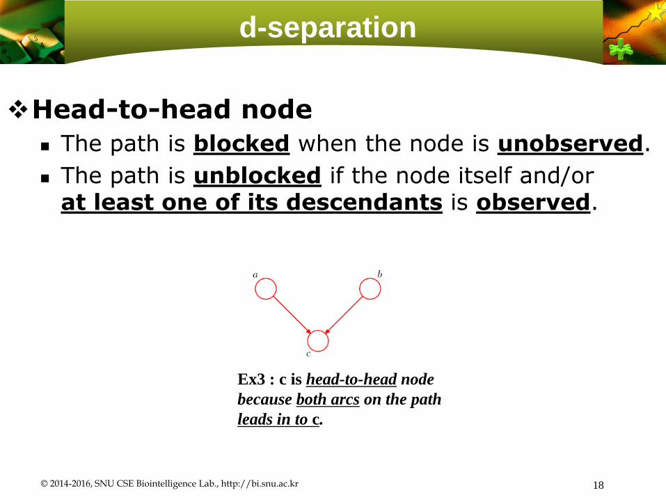
d-separation
Head-to-head node
The path is blocked when the node is unobserved.
The path is unblocked if the node itself and/or at least one of its descendants is observed.
© 2014-2016, SNU CSE Biointelligence Lab., http://bi.snu.ac.kr 18
Ex3 : c is head-to-head node
because both arcs on the path
leads in to c.

d-separation
d-separation?
All paths between two nodes(variables) are blocked.
The joint distribution will satisfy
conditional independence with respect toconcerned variables.
© 2014-2016, SNU CSE Biointelligence Lab., http://bi.snu.ac.kr 19

d-separation
© 2014-2016, SNU CSE Biointelligence Lab., http://bi.snu.ac.kr 20
(Evidence nodes are observed ones.)
Ex4 :
V_b1 is tail-to-tail node and is observed,
so it blocks the path.
V_b2 is head-to-tail node and is observed,
so it blocks the path.
V_b3 is head-to-head node and is
unobserved, so it blocks the path.
All the paths from V_i to V_j are blocked,
so they are conditionally independent.

D-Separation: 1st case
None of the variables are observed
The variable c is observed
The conditioned node ‘blocks’ the path from a to b, causes a and b to become (conditionally) independent.
© 2014-2016, SNU CSE Biointelligence Lab., http://bi.snu.ac.kr 21
Node c is tail-to-tail

D-Separation: 2nd case
None of the variables are observed
The variable c is observed
The conditioned node ‘blocks’ the path from a to b, causes a and b to become (conditionally) independent.
© 2014-2016, SNU CSE Biointelligence Lab., http://bi.snu.ac.kr 22
Node c is head-to-tail
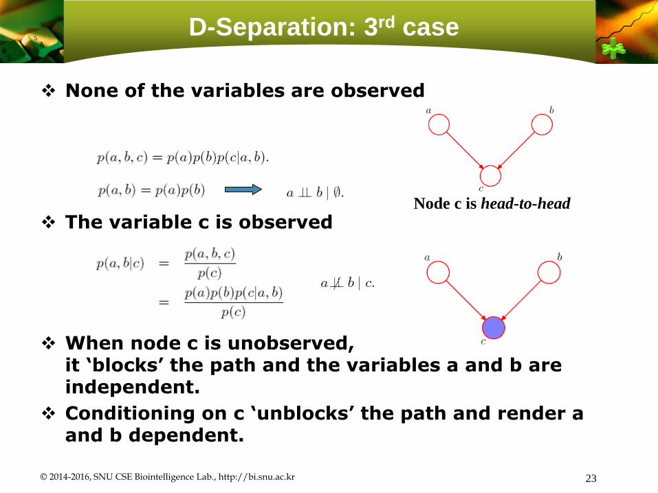
D-Separation: 3rd case
None of the variables are observed
The variable c is observed
When node c is unobserved, it ‘blocks’ the path and the variables a and b are independent.
Conditioning on c ‘unblocks’ the path and render a and b dependent.
© 2014-2016, SNU CSE Biointelligence Lab., http://bi.snu.ac.kr 23
Node c is head-to-head

Fuel gauge example
B – Battery, F-fuel, G-electric fuel gauge
Checking the fuel gauge
Checking the battery also has the meaning?
© 2014-2016, SNU CSE Biointelligence Lab., http://bi.snu.ac.kr 24
( Makes it more likely )
Makes it less likely than observation of fuel gauge only.
(rather unreliable fuel gauge)
(explaining away)

d-separation
(a) a is dependent to b given c
Head-to-head node e is unblocked, because a descendant c is in the conditioning set.
Tail-to-tail node f is unblocked
(b) a is independent to b given f
Head-to-head node e is blocked
Tail-to-tail node f is blocked
© 2014-2016, SNU CSE Biointelligence Lab., http://bi.snu.ac.kr 25
(C) 2000-2002 SNU CSE Biointelligence Lab 26
19.7 Probabilistic Inference in
Polytrees (1/2)
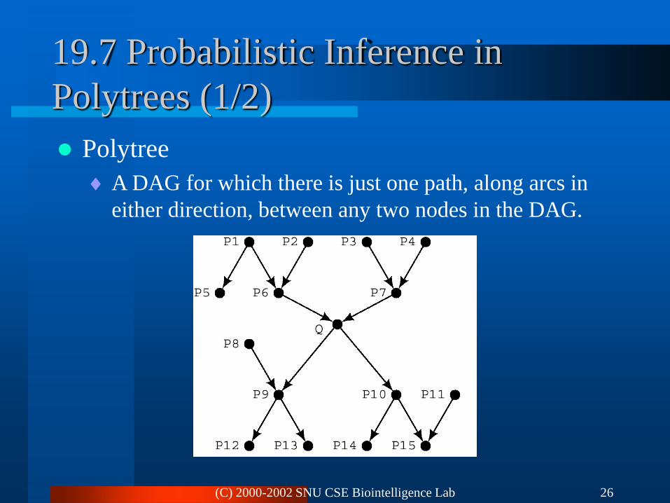
Polytree
A DAG for which there is just one path, along arcs in
either direction, between any two nodes in the DAG.
(C) 2000-2002 SNU CSE Biointelligence Lab 27
A node is above Q
The node is connected to Q only through Q’s parents
A node is below Q
The node is connected to Q only through Q’s immediate
successors.
Three types of evidence.
All evidence nodes are above Q.
All evidence nodes are below Q.
There are evidence nodes both above and below Q.
19.7 Probabilistic Inference in
Polytrees (2/2)
(C) 2000-2002 SNU CSE Biointelligence Lab 28
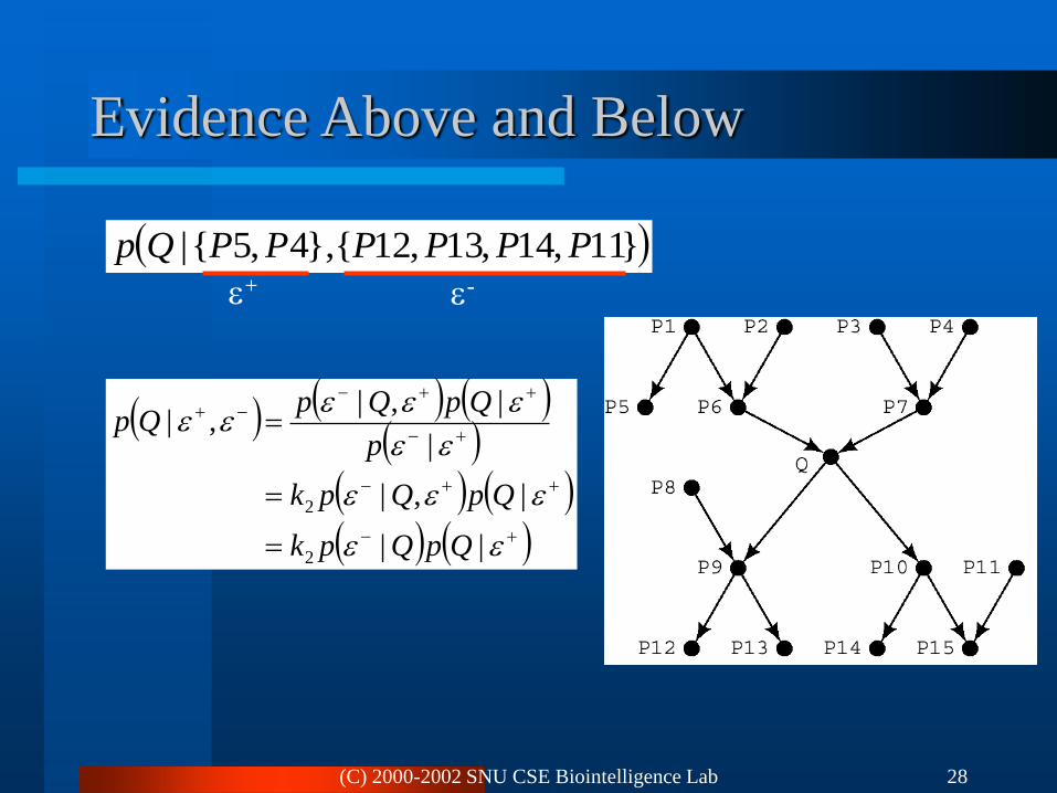
Evidence Above and Below
||
|,|
|
|,|,|
2
2
QpQpk
QpQpk
p
QpQpQp
}11,14,13,12{},4,5{| PPPPPPQp
+ -
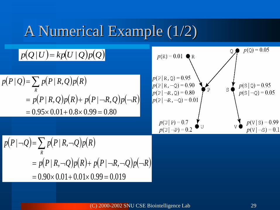
(C) 2000-2002 SNU CSE Biointelligence Lab 29
A Numerical Example (1/2)
QpQUkpUQp ||
80.099.08.001.095.0
,|,|
,||
RpQRPpRpQRPp
RpQRPpQPpR
019.099.001.001.090.0
,|,|
,||
RpQRPpRpQRPp
RpQRPpQPpR
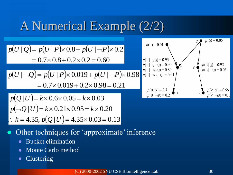
(C) 2000-2002 SNU CSE Biointelligence Lab 30
A Numerical Example (2/2)
Other techniques for ‘approximate’ inference
Bucket elimination
Monte Carlo method
Clustering
60.02.02.08.07.0
2.0|8.0||
PUpPUpQUp
21.098.02.0019.07.0
98.0|019.0||
PUpPUpQUp
13.003.035.4|,35.4
20.095.021.0|
03.005.06.0|
UQpk
kkUQp
kkUQp

Exercise
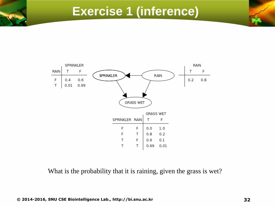
Exercise 1 (inference)
© 2014-2016, SNU CSE Biointelligence Lab., http://bi.snu.ac.kr 32
What is the probability that it is raining, given the grass is wet?

Exercise 2 (inference)
Q1) p(U|R,Q,S) =?
Q2) p(P|Q) = ?
Q3) p(Q|P) = ?
First, you may try to calculate by hand
Next, you can check the answer with GeNIe
© 2014-2016, SNU CSE Biointelligence Lab., http://bi.snu.ac.kr 33
Dataset for Exercise with GeNIe
Alarm Network
data_Alarm_modified.xdsl
Pima Indians Diabetes
discretization with Weka: pima_diabetes.arff
(result: pima_diabetes_supervised_discretized.csv)
Learning Bayesian network from data:
pima_diabetes_supervised_discretized.csv
© 2014-2016, SNU CSE Biointelligence Lab., http://bi.snu.ac.kr 34

Dataset #1: Alarm Network
Description
The network for a medical diagnostic system developed for on-line monitoring of patients in intensive care units
You will learn how to do inference with a given Bayesian network
Configuration of the data set
37 variables, discrete (2~4 levels)
Variables represent various states of heart, blood vessel and lung
Three kinds of variables
Diagnostic: basis of alarm
Measurement: observations
Intermediate: states of a patient
© 2014-2016, SNU CSE Biointelligence Lab., http://bi.snu.ac.kr 35
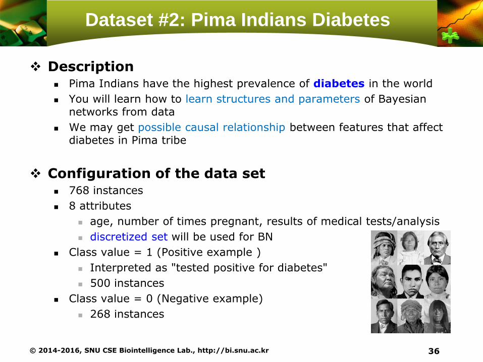
Dataset #2: Pima Indians Diabetes
Description Pima Indians have the highest prevalence of diabetes in the world
You will learn how to learn structures and parameters of Bayesian networks from data
We may get possible causal relationship between features that affect diabetes in Pima tribe
Configuration of the data set 768 instances
8 attributes
age, number of times pregnant, results of medical tests/analysis
discretized set will be used for BN
Class value = 1 (Positive example )
Interpreted as "tested positive for diabetes"
500 instances
Class value = 0 (Negative example)
268 instances
© 2014-2016, SNU CSE Biointelligence Lab., http://bi.snu.ac.kr 36
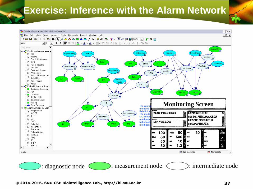
Exercise: Inference with the Alarm Network
© 2014-2016, SNU CSE Biointelligence Lab., http://bi.snu.ac.kr 37
: diagnostic node : measurement node : intermediate node
Monitoring Screen

Exercise: Inference with the Alarm Network
Inference tasks
Set evidences (according to observations or sensors)
‘Network – Update Beliefs’, or ‘F5’
© 2014-2016, SNU CSE Biointelligence Lab., http://bi.snu.ac.kr 38

Exercise: Inference with the Alarm Network
Inference tasks
Network - Probability of Evidence
© 2014-2016, SNU CSE Biointelligence Lab., http://bi.snu.ac.kr 39
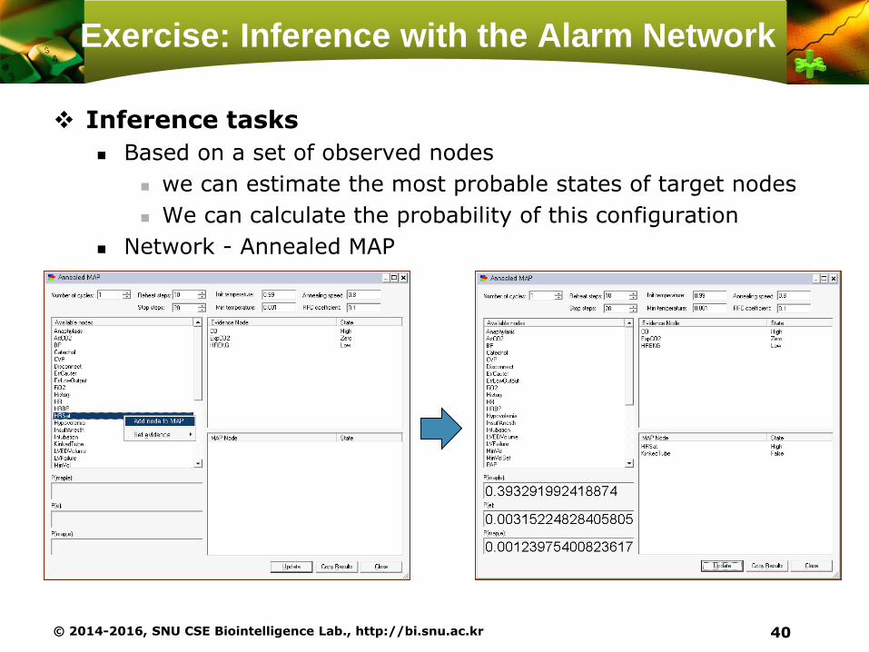
Exercise: Inference with the Alarm Network
Inference tasks
Based on a set of observed nodes
we can estimate the most probable states of target nodes
We can calculate the probability of this configuration
Network - Annealed MAP
© 2014-2016, SNU CSE Biointelligence Lab., http://bi.snu.ac.kr 40

Exercise: Learning from Diabetes data
Pima Indians Diabetes data
Step 1: discretization of real-valued features with Weka
© 2014-2016, SNU CSE Biointelligence Lab., http://bi.snu.ac.kr 41
1. Open ‘pima_diabetes.arff’
2. Apply ‘Filter-Supervised-Attribute-Discretize’
with default setting
3. Save into
‘pima_diabetes_supervised_discretized.csv’

Exercise: Learning from Diabetes data
Pima Indians Diabetes data
Step 2: Learning structure of the Bayesian network
© 2014-2016, SNU CSE Biointelligence Lab., http://bi.snu.ac.kr 42
1. File-Open Data File: pima_diabetes_supervised_discretized.csv
2. Data-Learn New Network
3. Set parameters as in Fig. 1
4. Edit the resulting graph: changing position, color
Fig. 1 Parameter setting Fig. 2 Learned structure
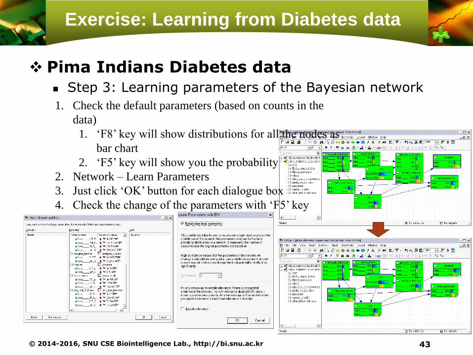
Exercise: Learning from Diabetes data
Pima Indians Diabetes data
Step 3: Learning parameters of the Bayesian network
© 2014-2016, SNU CSE Biointelligence Lab., http://bi.snu.ac.kr 43
1. Check the default parameters (based on counts in the
data)
1. ‘F8’ key will show distributions for all the nodes as
bar chart
2. ‘F5’ key will show you the probability
2. Network – Learn Parameters
3. Just click ‘OK’ button for each dialogue box
4. Check the change of the parameters with ‘F5’ key

- AI & UNCERTAINTY
- BAYESIAN NETWORKS IN DETAIL
Appendix
© 2014-2016, SNU CSE Biointelligence Lab., http://bi.snu.ac.kr 44

AI & Uncertainty
Probability
Probability plays a central role in modern pattern
recognition.
The main tool to deal uncertainties
All of the probabilistic inference and learning amount to
repeated application of the sum rule and the product rule
© 2014-2016, SNU CSE Biointelligence Lab., http://bi.snu.ac.kr 46
Random Variables: variables + probability

Artificial Intelligence (AI)
The objective of AI is to build intelligent computers
We want intelligent, adaptive, robust behavior
Often hand programming not possible.
Solution? Get the computer to program itself, by
showing it examples of the behavior we want!
This is the learning approach to AI.
© 2014-2016, SNU CSE Biointelligence Lab., http://bi.snu.ac.kr 47
cat car

Artificial Intelligence (AI)
(Traditional) AI
Knowledge & reasoning; work with facts/assertions;
develop rules of logical inference
Planning: work with applicability/effects of actions;
develop searches for actions which achieve goals/avert
disasters.
Expert systems: develop by hand a set of rules for
examining inputs, updating internal states and
generating outputs
© 2014-2016, SNU CSE Biointelligence Lab., http://bi.snu.ac.kr 48

Artificial Intelligence (AI)
Probabilistic AI emphasis on noisy measurements, approximation in hard
cases, learning, algorithmic issues.
The power of learning Automatic system building
old expert systems needed hand coding of knowledge and of output semantics
learning automatically constructs rules and supports all types of queries
Probabilistic databases
traditional DB technology cannot answer queries about items that were never loaded into the dataset
UAI models are like probabilistic databases
© 2014-2016, SNU CSE Biointelligence Lab., http://bi.snu.ac.kr 49

Uncertainty and Artificial Intelligence
(UAI)
Probabilistic methods can be used to:
make decisions given partial information about the world
account for noisy sensors or actuators
explain phenomena not part of our models
describe inherently stochastic behavior in the world
© 2014-2016, SNU CSE Biointelligence Lab., http://bi.snu.ac.kr 50
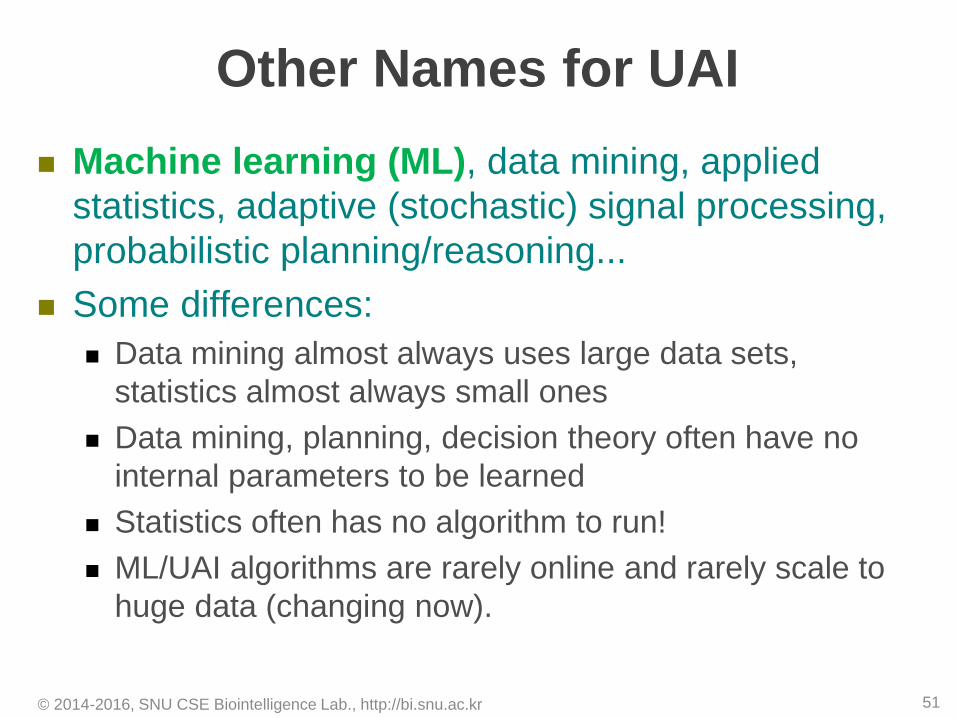
Other Names for UAI
Machine learning (ML), data mining, applied
statistics, adaptive (stochastic) signal processing,
probabilistic planning/reasoning...
Some differences:
Data mining almost always uses large data sets,
statistics almost always small ones
Data mining, planning, decision theory often have no
internal parameters to be learned
Statistics often has no algorithm to run!
ML/UAI algorithms are rarely online and rarely scale to
huge data (changing now).
© 2014-2016, SNU CSE Biointelligence Lab., http://bi.snu.ac.kr 51

Learning in AI
Learning is most useful
when the structure of the task is not well understood
but can be characterized by a dataset with strong
statistical regularity
Also useful in adaptive or dynamic situations when
the task (or its parameters) are constantly
changing
Currently, these are challenging topics of machine
learning and data mining research
© 2014-2016, SNU CSE Biointelligence Lab., http://bi.snu.ac.kr 52
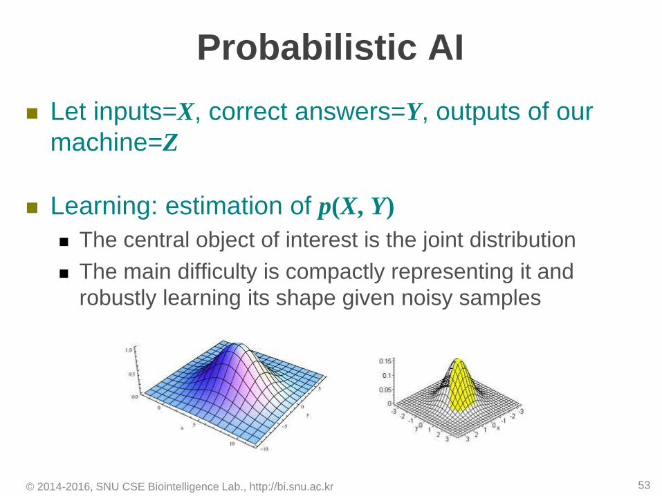
Probabilistic AI
Let inputs=X, correct answers=Y, outputs of our
machine=Z
Learning: estimation of p(X, Y)
The central object of interest is the joint distribution
The main difficulty is compactly representing it and
robustly learning its shape given noisy samples
© 2014-2016, SNU CSE Biointelligence Lab., http://bi.snu.ac.kr 53
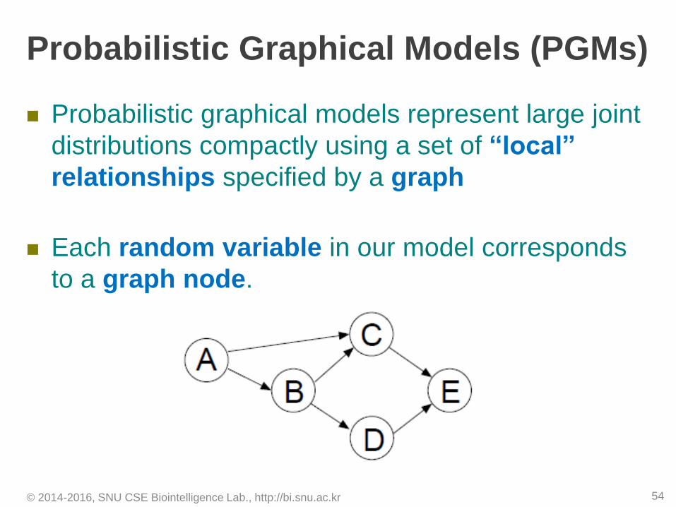
Probabilistic Graphical Models (PGMs)
Probabilistic graphical models represent large joint
distributions compactly using a set of “local”
relationships specified by a graph
Each random variable in our model corresponds
to a graph node.
© 2014-2016, SNU CSE Biointelligence Lab., http://bi.snu.ac.kr 54

Probabilistic Graphical Models (PGMs)
There are useful properties in using probabilistic graphical models A simple way to visualize the structure of a probabilistic
model
Insights into the properties of the model
Complex computations (for inference and learning) can be expressed in terms of graphical manipulations underlying mathematical expressions
© 2014-2016, SNU CSE Biointelligence Lab., http://bi.snu.ac.kr 55
56
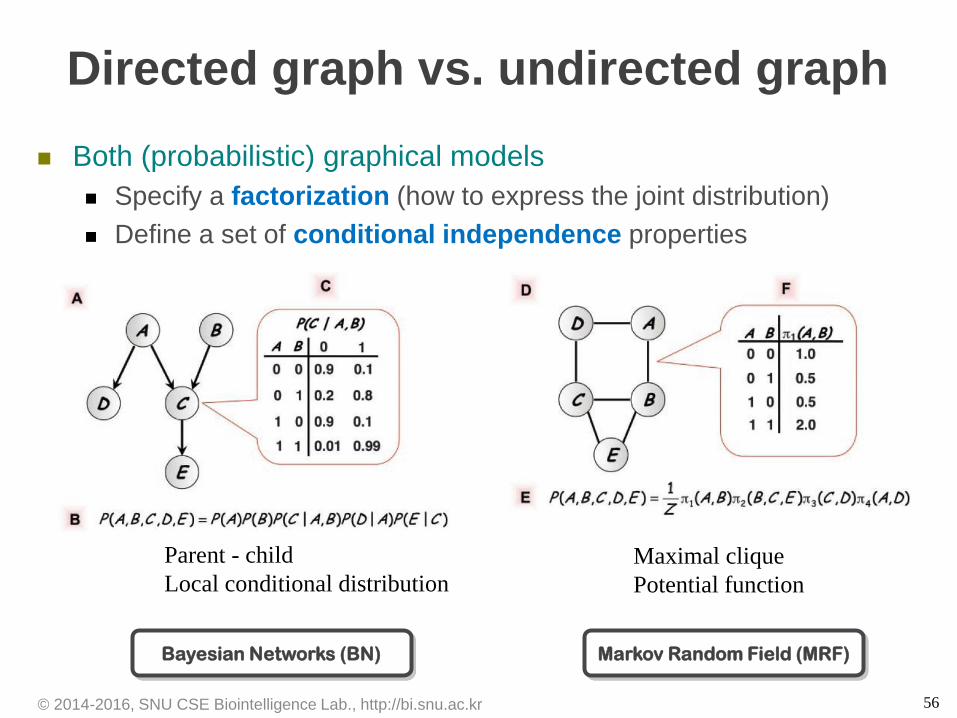
Directed graph vs. undirected graph
Both (probabilistic) graphical models
Specify a factorization (how to express the joint distribution)
Define a set of conditional independence properties
Parent - child
Local conditional distribution
Maximal clique
Potential function
© 2014-2016, SNU CSE Biointelligence Lab., http://bi.snu.ac.kr
Bayesian Networks (BN) Markov Random Field (MRF)
Bayesian Networks in Detail

© 2014-2016, SNU CSE Biointelligence Lab., http://bi.snu.ac.kr 58
(DAG)
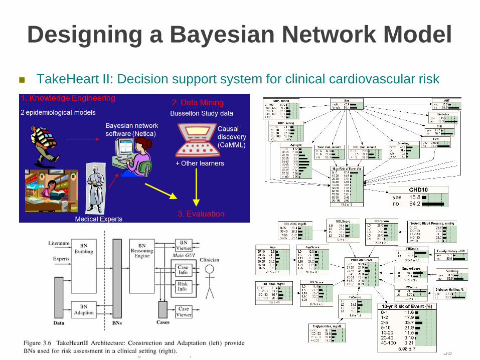
Designing a Bayesian Network Model
TakeHeart II: Decision support system for clinical cardiovascular risk
assessment
© 2014-2016, SNU CSE Biointelligence Lab., http://bi.snu.ac.kr 59
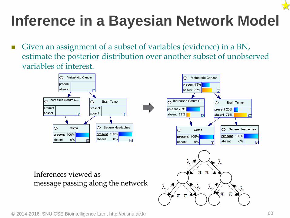
Inference in a Bayesian Network Model
Given an assignment of a subset of variables (evidence) in a BN, estimate the posterior distribution over another subset of unobserved variables of interest.
© 2014-2016, SNU CSE Biointelligence Lab., http://bi.snu.ac.kr 60
Inferences viewed as message passing along the network
Bayesian Networks
The joint distribution defined by a graph is given by the
product of a conditional distribution of each node
conditioned on their parent nodes.
© 2014-2016, SNU CSE Biointelligence Lab., http://bi.snu.ac.kr 61
𝑝 𝑥1, 𝑥2, … , 𝑥7 =
(𝑃𝑎(𝑥𝑘) denotes the set of parents of xk)
K
kkk xPaxpp
1
))(|()(x
ex)
* Without given DAG structure, usual chain rule can be applied to get
the joint distribution. But computational cost is much higher.
Bayes’ Theorem
© 2014-2016, SNU CSE Biointelligence Lab., http://bi.snu.ac.kr 62
( | ) ( )( | )
( )
p X Y p Yp Y X
p X
( ) ( | ) ( )Y
p X p X Y p Y
Posterior
Likelihood
Prior
Normalizing
constant
posterior likelihood × prior

Bayes’ Theorem
© 2014-2016, SNU CSE Biointelligence Lab., http://bi.snu.ac.kr 63
Figure from Figure 1. in (Adams, et all, 2013)
obtained from http://journal.frontiersin.org/article/10.3389/fpsyt.2013.00047/full

Bayesian Probabilities-Frequentist vs. Bayesian
Likelihood:
Frequentist w: a fixed parameter determined by ‘estimator’
Maximum likelihood: Error function =
Error bars: Obtained by the distribution of possible data sets Bootstrap
Cross-validation
Bayesian a probability distribution w: the uncertainty in the parameters
Prior knowledge Noninformative (uniform) prior, Laplace correction in estimating priors
Monte Carlo methods, variational Bayes, EP
© 2014-2016, SNU CSE Biointelligence Lab., http://bi.snu.ac.kr 64
( | ) ( )( | )
( )
p pp
p
w ww
DD
D
( | )p wD
log ( | )p wDD
Thomas Bayes
(See an article ‘WHERE Do PROBABILITIES COME FROM?’ on page 491 in the textbook (Russell and Norvig, 2010) for more discussion)
Conditional Independence
Conditional independence simplifies both the structure of a model and
the computations
An important feature of graphical models is that conditional
independence properties of the joint distribution can be read directly
from the graph without having to perform any analytical manipulations
The general framework for this is called d-separation
© 2014-2016, SNU CSE Biointelligence Lab., http://bi.snu.ac.kr 65

Three example graphs – 1st case
None of the variables are observed
The variable c is observed
The conditioned node ‘blocks’ the path from a to b,
causes a and b to become (conditionally) independent.
© 2014-2016, SNU CSE Biointelligence Lab., http://bi.snu.ac.kr 66
Node c is tail-to-tail
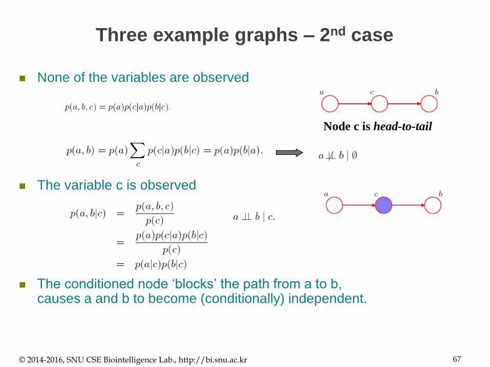
Three example graphs – 2nd case
None of the variables are observed
The variable c is observed
The conditioned node ‘blocks’ the path from a to b, causes a and b to become (conditionally) independent.
© 2014-2016, SNU CSE Biointelligence Lab., http://bi.snu.ac.kr 67
Node c is head-to-tail

Three example graphs – 3rd case
None of the variables are observed
The variable c is observed
When node c is unobserved,
it ‘blocks’ the path and the variables a and b are independent.
Conditioning on c ‘unblocks’ the path and render a and b dependent.
© 2014-2016, SNU CSE Biointelligence Lab., http://bi.snu.ac.kr 68
Node c is head-to-head

Three example graphs - Fuel gauge example
B – Battery, F-fuel, G-electric fuel gauge
Checking the fuel gauge
Checking the battery also has the meaning?
© 2014-2016, SNU CSE Biointelligence Lab., http://bi.snu.ac.kr 69
( Makes it more likely )
Makes it less likely than observation of fuel gauge only.
(rather unreliable fuel gauge)
(explaining away)
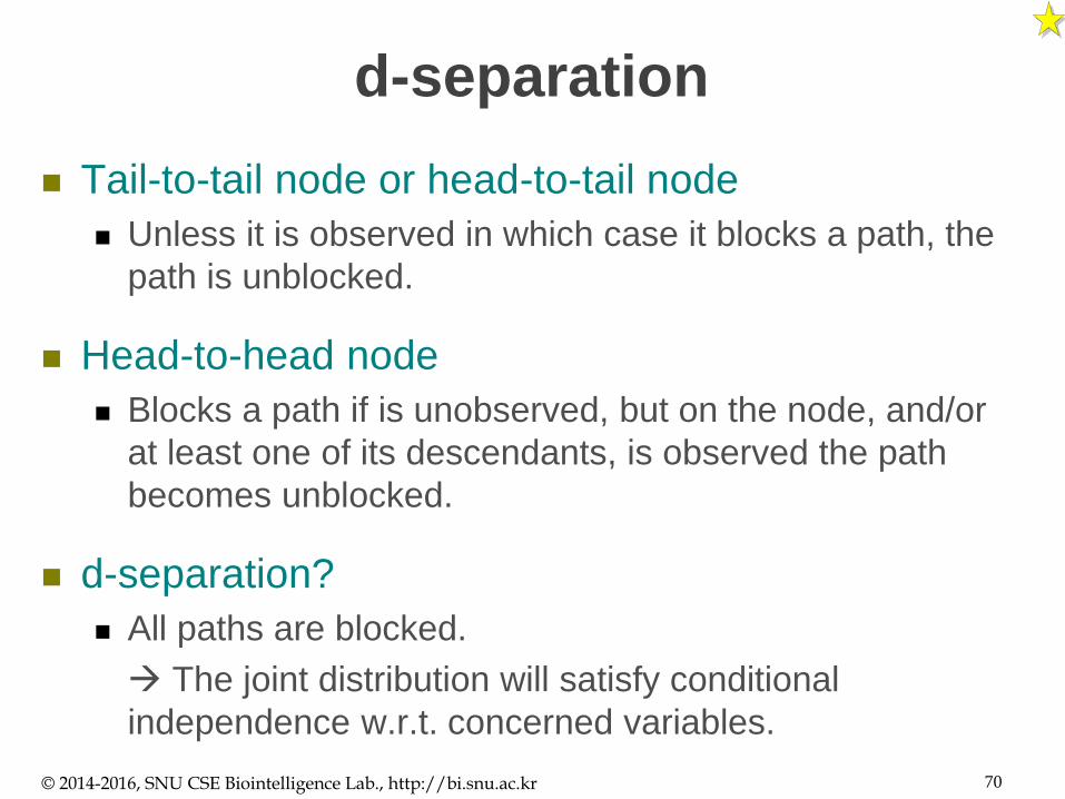
d-separation
Tail-to-tail node or head-to-tail node
Unless it is observed in which case it blocks a path, the
path is unblocked.
Head-to-head node
Blocks a path if is unobserved, but on the node, and/or
at least one of its descendants, is observed the path
becomes unblocked.
d-separation?
All paths are blocked.
The joint distribution will satisfy conditional
independence w.r.t. concerned variables.
© 2014-2016, SNU CSE Biointelligence Lab., http://bi.snu.ac.kr 70
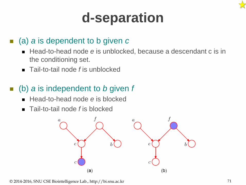
d-separation
(a) a is dependent to b given c
Head-to-head node e is unblocked, because a descendant c is in
the conditioning set.
Tail-to-tail node f is unblocked
(b) a is independent to b given f
Head-to-head node e is blocked
Tail-to-tail node f is blocked
© 2014-2016, SNU CSE Biointelligence Lab., http://bi.snu.ac.kr 71

d-separation
Another example of conditional independence and d-separation: i.i.d.
(independent identically distributed) data
Problem: finding posterior dist. for the mean of a univariate Gaussian dist.
Every path is blocked and so the observations D={x1,…,xN} are independent
given
© 2014-2016, SNU CSE Biointelligence Lab., http://bi.snu.ac.kr 72
(The observations are in general no longer independent!)
(independent)

d-separation
Naïve Bayes model
Key assumption: conditioned on the class z, the distribution of the
input variables x1,…, xD are independent.
Input {x1,…,xN} with their class labels,
then we can fit the naïve Bayes model to the training data using
maximum likelihood assuming that the data are drawn
independently from the model.
© 2014-2016, SNU CSE Biointelligence Lab., http://bi.snu.ac.kr 73
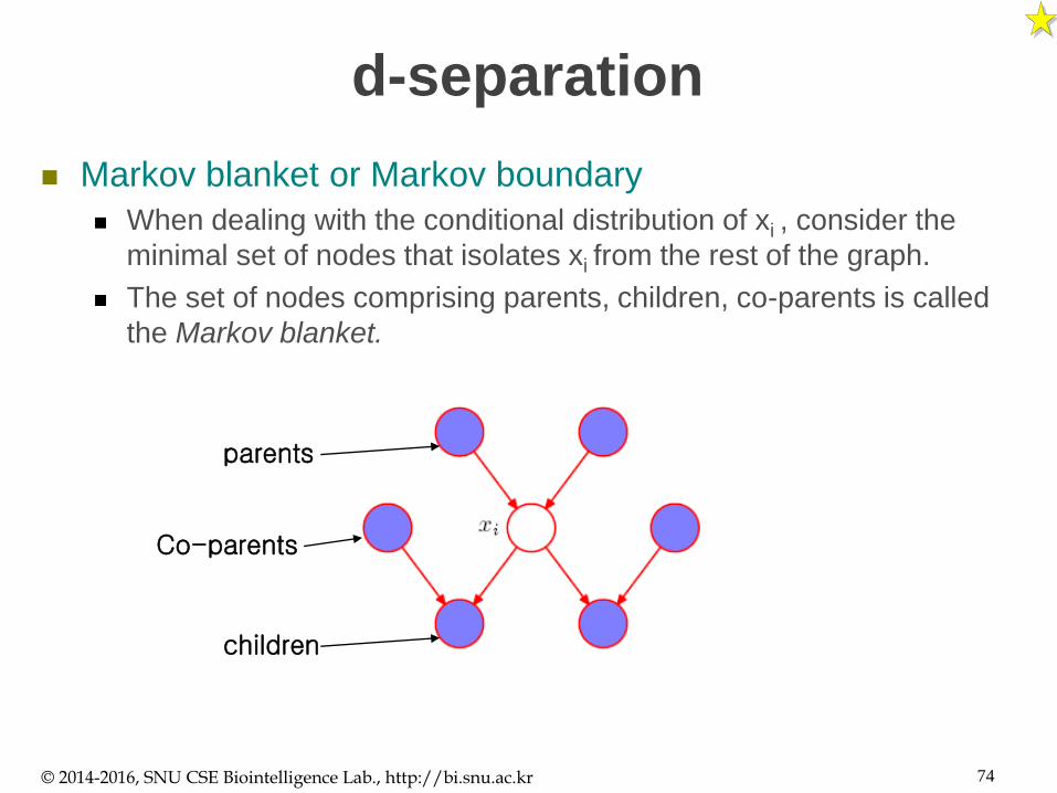
d-separation
Markov blanket or Markov boundary
When dealing with the conditional distribution of xi , consider the
minimal set of nodes that isolates xi from the rest of the graph.
The set of nodes comprising parents, children, co-parents is called
the Markov blanket.
© 2014-2016, SNU CSE Biointelligence Lab., http://bi.snu.ac.kr 74
Co-parents
parents
children

Probability Distributions
Discrete variables Beta, Bernoulli, binomial
Dirichlet, multinomial
…
Continuous variables Normal (Gaussian)
Student-t
…
Exponential family & conjugacy Many probability densities on x can be represented as the same form
There are conjugate family of density functions having the same form of density functions
Beta & binomial
Dirichlet & multinomial
Normal & Normal
© 2014-2016, SNU CSE Biointelligence Lab., http://bi.snu.ac.kr 75
( | ) ( ) ( ) exp ( )Tp h g x x u x
beta Dirichlet
binomial Gaussian
F
x
beta
binomial
Dirichlet
multinomial
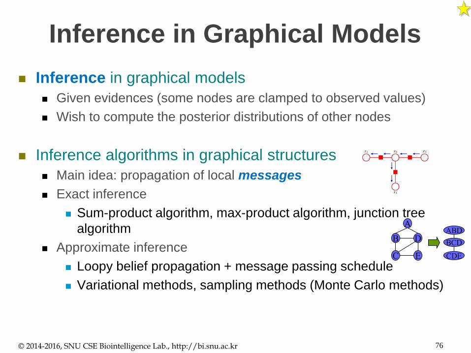
Inference in Graphical Models
Inference in graphical models
Given evidences (some nodes are clamped to observed values)
Wish to compute the posterior distributions of other nodes
Inference algorithms in graphical structures
Main idea: propagation of local messages
Exact inference
Sum-product algorithm, max-product algorithm, junction tree
algorithm
Approximate inference
Loopy belief propagation + message passing schedule
Variational methods, sampling methods (Monte Carlo methods)
© 2014-2016, SNU CSE Biointelligence Lab., http://bi.snu.ac.kr 76
A
B D
C E
ABD
BCD
CDE
Learning Parameters of
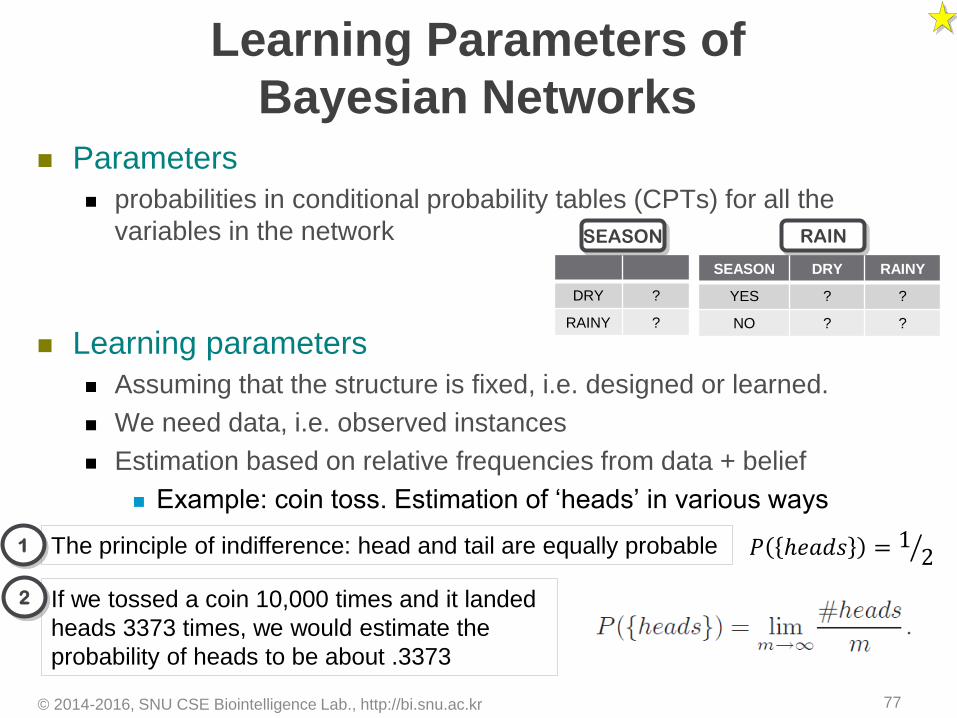
Bayesian Networks Parameters
probabilities in conditional probability tables (CPTs) for all the
variables in the network
Learning parameters
Assuming that the structure is fixed, i.e. designed or learned.
We need data, i.e. observed instances
Estimation based on relative frequencies from data + belief
Example: coin toss. Estimation of ‘heads’ in various ways
© 2014-2016, SNU CSE Biointelligence Lab., http://bi.snu.ac.kr 77
SEASON DRY RAINY
YES ? ?
NO ? ?
RAIN
DRY ?
RAINY ?
SEASON
The principle of indifference: head and tail are equally probable
If we tossed a coin 10,000 times and it landed
heads 3373 times, we would estimate the
probability of heads to be about .3373
𝑃 ℎ𝑒𝑎𝑑𝑠 = 1 21
2
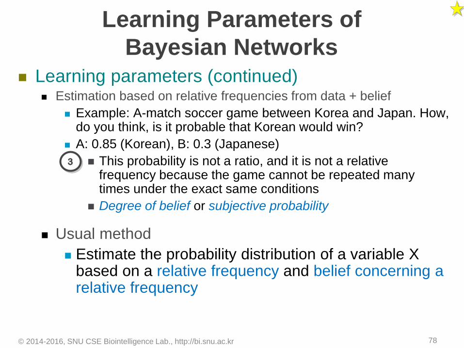
Learning Parameters of
Bayesian Networks Learning parameters (continued)
Estimation based on relative frequencies from data + belief
Example: A-match soccer game between Korea and Japan. How, do you think, is it probable that Korean would win?
A: 0.85 (Korean), B: 0.3 (Japanese)
This probability is not a ratio, and it is not a relative frequency because the game cannot be repeated many times under the exact same conditions
Degree of belief or subjective probability
Usual method
Estimate the probability distribution of a variable X based on a relative frequency and belief concerning a relative frequency
© 2014-2016, SNU CSE Biointelligence Lab., http://bi.snu.ac.kr 78
3

Learning Parameters of
Bayesian Networks Simple ‘counting’ solution (Bayesian point of view)
Parameter estimation of a single node
Assume local parameter independence
For a binary variable (for example, a coin toss)
prior: Beta distribution - Beta(a,b)
after we have observed m heads and N-m tails posterior -
Beta(a+m,b+N-m) and 𝑃 𝑋 = ℎ𝑒𝑎𝑑 = (𝑎+𝑚)𝑁
© 2014-2016, SNU CSE Biointelligence Lab., http://bi.snu.ac.kr 79
(conjugacy of Beta and Binomial distributions)
betabinomial

Learning Parameters of
Bayesian Networks Simple ‘counting’ solution (Bayesian point of view)
For a multinomial variable (for example, a dice toss)
prior: Dirichlet distribution – Dirichlet(a1,a2, …, ad)
𝑃 𝑋 = 𝑘 = 𝑎𝑘𝑁 𝑁 = 𝑎𝑘
Observing state i: Dirichlet(a1,…,ai+1,…, ad)
For an entire network
We simply iterate over its nodes
In the case of incomplete data
In real data, many of the variable values may be incorrect or missing
Usual approximating solution is given by Gibbs sampling or EM
(expectation maximization) technique
© 2014-2016, SNU CSE Biointelligence Lab., http://bi.snu.ac.kr 80
(conjugacy of Dirichlet and Multinomial distributions)

Learning Parameters of
Bayesian Networks Smoothing
Another viewpoint
Laplace smoothing or additive smoothing given observed counts for
d states of a variable 𝑋 = (𝑥1, 𝑥2,…𝑥𝑑)
From a Bayesian point of view, this corresponds to the expected
value of the posterior distribution, using a symmetric Dirichlet
distribution with parameter α as a prior.
Additive smoothing is commonly a component of naive Bayes
classifiers.
© 2014-2016, SNU CSE Biointelligence Lab., http://bi.snu.ac.kr 81
𝑃 𝑋 = 𝑘 =𝑥𝑘 + 𝛼
𝑁 + 𝛼𝑑𝑖 = 1,… , 𝑑 , (𝛼 = 𝛼1 = 𝛼2 = ⋯𝛼𝑑)

Learning the Graph Structure
Learning the graph structure itself from data requires A space of possible structures
A measure that can be used to score each structure
From a Bayesian viewpoint
Tough points Marginalization over latent variables => challenging computational
problem
Exploring the space of structures can also be problematic The # of different graph structures grows exponentially with the # of
nodes
Usually we resort to heuristics Local score based, global score based, conditional independence test based, …
© 2014-2016, SNU CSE Biointelligence Lab., http://bi.snu.ac.kr 82
: score for each model
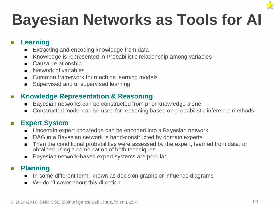
Bayesian Networks as Tools for AI
Learning Extracting and encoding knowledge from data
Knowledge is represented in Probabilistic relationship among variables
Causal relationship
Network of variables
Common framework for machine learning models
Supervised and unsupervised learning
Knowledge Representation & Reasoning Bayesian networks can be constructed from prior knowledge alone
Constructed model can be used for reasoning based on probabilistic inference methods
Expert System Uncertain expert knowledge can be encoded into a Bayesian network
DAG in a Bayesian network is hand-constructed by domain experts
Then the conditional probabilities were assessed by the expert, learned from data, or obtained using a combination of both techniques.
Bayesian network-based expert systems are popular
Planning In some different form, known as decision graphs or influence diagrams
We don’t cover about this direction
© 2014-2016, SNU CSE Biointelligence Lab., http://bi.snu.ac.kr 83
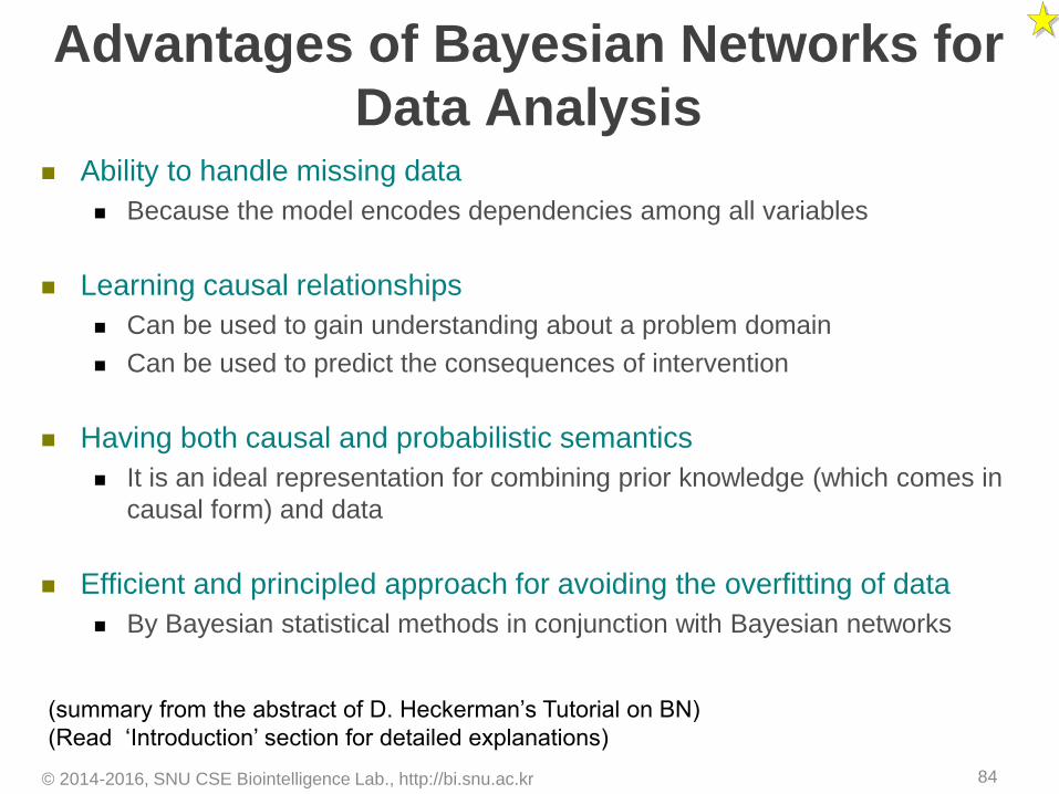
Advantages of Bayesian Networks for
Data Analysis Ability to handle missing data
Because the model encodes dependencies among all variables
Learning causal relationships
Can be used to gain understanding about a problem domain
Can be used to predict the consequences of intervention
Having both causal and probabilistic semantics
It is an ideal representation for combining prior knowledge (which comes in
causal form) and data
Efficient and principled approach for avoiding the overfitting of data
By Bayesian statistical methods in conjunction with Bayesian networks
© 2014-2016, SNU CSE Biointelligence Lab., http://bi.snu.ac.kr 84
(summary from the abstract of D. Heckerman’s Tutorial on BN)
(Read ‘Introduction’ section for detailed explanations)
References
K. Mohan & J. Pearl, UAI ’12 Tutorial on Graphical Models for Causal
Inference
S. Roweis, MLSS ’05 Lecture on Probabilistic Graphical Models
Chapter 1, Chapter 2, Chapter 8 (Graphical Models), in Pattern
Recognition and Machine Learning by C.M. Bishop, 2006.
David Heckerman, A Tutorial on Learning with Bayesian Networks.
R.E. Neapolitan, Learning Bayesian Networks, Pearson Prentice Hall,
2004.
© 2014-2016, SNU CSE Biointelligence Lab., http://bi.snu.ac.kr 85

More Textbooks and Courses
https://www.coursera.org/course/pgm :
Probabilistic Graphical Models by D. Koller
© 2014-2016, SNU CSE Biointelligence Lab., http://bi.snu.ac.kr 86


