154
Helge Langseth Bayesian Networks with Applications in Reliability Analysis Dr. Ing. Thesis Department of Mathematical Sciences Norwegian University of Science and Technology 2002

Helge Langseth
Bayesian Networkswith Applications in Reliability Analysis
Dr. Ing. Thesis
Department of Mathematical Sciences
Norwegian University of Science and Technology
2002


Preface
This thesis is submitted in partial fulfillment of the requirements for the degree “DoktorIngeniør” (Dr.Ing.) at the Norwegian University of Science and Technology (NTNU). Thework is financed by a scholarship from the Norwegian Research Council of Norway.
I would like to thank my supervisors Bo Lindqvist and Agnar Aamodt for their guidanceand support. I would also like to thank the members of the Decision Support SystemsGroup at Aalborg University for teaching me most of what I know about Bayesian net-works and influence diagrams. My stay in Denmark from August 1999 to July 2001 wasa wonderful period, and a special thanks to Thomas D. Nielsen, Finn Verner Jensen andOlav Bangsø for making those years so memorable. Furthermore, I would like to thankmy co-authors Agnar Aamodt, Olav Bangsø, Finn Verner Jensen, Uffe Kjærulff, BrianKristiansen, Bo Lindqvist, Thomas D. Nielsen, Claus Skaanning, Jirı Vomlel, Marta Vom-lelova, and Ole Martin Winnem for inspiring cooperation. Finally, I would like to thankMona for keeping up with me over the last couple of years. Her part in this work is largerthan anybody (including myself, unfortunately) will ever know.
Trondheim, October 2002
Helge Langseth

iv
List of papers
The thesis consists of the following 5 papers:
Paper I: Helge Langseth and Bo Henry Lindqvist: A maintenance model for compo-nents exposed to several failure modes and imperfect repair. TechnicalReport Statistics 10/2002, Department of Mathematical Sciences, Norwe-gian University of Science and Technology. Submitted as an invited paperto Mathematical and Statistical Methods in Reliability Kjell Doksum andBo Henry Lindqvist (Eds.), 2002.
Paper II: Helge Langseth and Finn Verner Jensen: Decision theoretic troubleshootingof coherent systems. Reliability Engineering and System Safety. Forth-coming, 2002.
Paper III: Helge Langseth and Thomas D. Nielsen: Classification using hierarchicalnaıve Bayes models. Technical Report TR-02-004, Department of Com-puter Science, Aalborg University, Denmark, 2002.
Paper IV: Helge Langseth and Olav Bangsø: Parameter learning in object orientedBayesian networks. Annals of Mathematics and Artificial Intelligence, 32(1/4):221–243, 2001.
Paper V: Helge Langseth and Thomas D. Nielsen: Fusion of domain knowledge withdata for structural learning in object oriented domains. Journal of MachineLearning Research. Forthcoming, 2002.
The papers are selected to cover most of the work I have been involved in over the lastyears, but s.t. they all share the same core: Bayesian network technology with possibleapplications in reliability analysis.
All papers can be read independently of each other, although Paper IV and Paper V areclosely related. Paper I is concerned with building a model for maintenance optimization;it is written for an audience of reliability data analysts. Papers II – V are related toproblem solving (Paper II and Paper III) and estimation (Paper IV and Paper V) usingthe Bayesian network formalism. These papers are written for an audience familiar withboth computer science as well as statistics, but with a terminology mostly collected fromthe computer scientists’ vocabulary.
v

vi

Background
Reliability analysis is deeply rooted in models for time to failure (survival analysis). Theanalysis of such time-to-event data arises in many fields, including medicine, actuarialsciences, economics, biology, public health and engineering. The Bayesian paradigm hasplayed an important role in survival analysis because the time-to-event data can be sparseand heavily censored. The statistical models must therefore in part be based on expertjudgement where a priori knowledge is combined with quantitative information repre-sented by data (Martz and Waller 1982; Ibrahim et al. 2001), see also (Gelman et al.1995). Bayesian approaches to survival analysis has lately received quite some attentiondue to recent advances in computational and modelling techniques (commonly referred toas computer-intensive statistical methods), and Bayesian techniques like flexible hierarchi-cal models have for example become common in reliability analysis.
Reliability models of repairable systems often become complex, and they may be difficultto build using traditional frameworks. Additionally, reliability analyses that historicallywere mostly conducted for documentation purposes are now used as direct input to complexdecision problems. The complexity of these decision problems can lead to a situation wherethe decision maker looses his overview, which in turn can lead to sub-optimal decisions.This has paved the way for formalisms that offer a transparent yet mathematically soundmodelling framework; the statistical models must build on simple semantics (to interactwith domain experts and the decision maker) and at the same time offer the mathematicalfinesse required to model the actual decision problem at hand.
The framework employed in this thesis is (discrete) Bayesian networks (BNs); BNs aredescribed in (Pearl 1988; Jensen 1996; Lauritzen 1996; Cowell et al. 1999; Jensen 2001).A discrete BN encodes the probability mass function governing a set X1, . . . , Xn ofdiscrete random variables by specifying a set of conditional independence assumptionstogether with a set of conditional probability tables (CPTs). More specifically, a BNconsists of a qualitative part; a directed acyclic graph where the nodes mirror the randomvariables Xi, and a quantitative part; the set of CPTs. We call the nodes with outgoingedges directed into a specific node the parents of that node, and say that a node Xj is adescendant of Xi if and only if there is a directed path from Xi to Xj in the graph. Now, theedges of the graph represent the assertion that a variable is conditionally independent of itsnon-descendants in the graph given its parents (other conditional independence statementscan be read off the graph using d-separation rules (Pearl 1988)). Next, a CPT is specifiedfor each variable, describing the conditional probability mass for that variable given thestate of its parents. Note that a BN can represent any probability mass function, andthrough its factorized representation it does so in a cost-efficient manner (wrt. the numberof parameters required to describe the probability mass function).
The most important task in a BN is inference, i.e., to calculate conditional probabilities oversome target variables conditioned on the observed values of other variables (for examplethe probability of a system being broken given the state of some of its components). Both
vii

exact as well as approximate inference in a BN is in general NP-hard (Cooper 1990; Dagumand Luby 1993), but fortunately both exact propagation-algorithms (Shafer and Shenoy1990; Jensen et al. 1990; Jensen 1996) as well as MCMC simulation (Geman and Geman1984; Gilks et al. 1994; Gilks et al. 1996) have shown useful in practice.
The Bayesian formalism offers an intuitive way to estimate models based on the combina-tion of statistical data and expert judgement. For a given graphical structure, estimationof the conditional probability tables was considered by Spiegelhalter and Lauritzen (1990),who showed how the full posterior distribution over the parameter-space can be obtainedin closed form by local computations. The EM-algorithm by Dempster et al. (1977) is par-ticularly intuitive in BN models, as the sufficient statistics required for parameter learningare available in the cliques after propagation (Lauritzen 1995). The EM-algorithm can alsobe used to find MAP-parameters (Green 1990). Structural learning, i.e., to estimate thegraphical structure of a BN (the edges of the graph), is considered in (Cooper and Her-skovits 1992; Heckerman et al. 1995; Friedman 1998). A BN structure constrains the setof possible CPTs by defining their scopes, and this is utilized in (Cooper and Herskovits1992), where it is shown how a posterior distribution over the space of directed acyclicgraphs can be obtained through local computations. Heckerman et al. (1995) examine theusage of priors over the model-space, and empirically investigate the use of (stochastic)search over this space. Friedman (1998) extends these results to cope with missing data.
The fast inference algorithms and simple semantics of the BN models have lead to acontinuous trend of building increasingly larger BN models. Such large models can betime consuming to build and maintain, and this problem is attacked by defining special“types” of BNs tailor-made for complex domains: Both (Koller and Pfeffer 1997) as well as(Bangsø and Wuillemin 2000) describe modelling languages where repetitive substructuresplay an important role during model building; these frameworks are called object orientedBNs. A language for probabilistic frame-based systems is proposed in (Koller and Pfeffer1998), and rational models (i.e., models associated with a relational domain structure asdefined for instance by a relational database) is described in (Getoor et al. 2001).
Historically, BNs have been used in two quite different settings in the safety and reliabilitysciences. The first body of work uses BNs solely as a tool for building complex statisticalmodels. Analysis of lifetime data, models to extend the flexibility of classical reliabilitytechniques (such as fault trees and reliability block diagrams), fault finding systems, andmodels for human errors and organizational factors all fall into this category. On the otherhand, some researchers regard BNs as causal Markov models, and use them in for exampleaccident investigation. The recent book by Pearl (2000), see also (Spirtes et al. 1993), givesa clear exposition of BNs as causal models, and although statisticians have traditionallybeen reluctant to the use of causal models (Speed (1990) wrote: “Considerations of causal-ity should be treated as they have always been treated in statistics: preferably not at allbut, if necessary, then with great care.”) a statistical treatment of causal mechanisms andcausal inference in association with Bayesian networks and influence diagrams is startingto dawn, see e.g., (Lauritzen 2001; Dawid 2002).
viii

Summary
A common goal of the papers in this thesis is to propose, formalize and exemplify the useof Bayesian networks as a modelling tool in reliability analysis. The papers span work inwhich Bayesian networks are merely used as a modelling tool (Paper I), work where modelsare specially designed to utilize the inference algorithms of Bayesian networks (Paper II andPaper III), and work where the focus has been on extending the applicability of Bayesiannetworks to very large domains (Paper IV and Paper V).
Paper I is in this respect an application paper, where model building, estimation andinference in a complex time-evolving model is simplified by focusing on the conditionalindependence statements embedded in the model; it is written with the reliability dataanalyst in mind. We investigate the mathematical modelling of maintenance and repairof components that can fail due to a variety of failure mechanisms. Our motivation is tobuild a model, which can be used to unveil aspects of the “quality” of the maintenanceperformed. This “quality” is measured by two groups of model parameters: The firstmeasures “eagerness”, the maintenance crew’s ability to perform maintenance at the righttime to try to stop an evolving failure; the second measures “thoroughness”, the crew’sability to actually stop the failure development. The model we propose is motivated by theimperfect repair model of Brown and Proschan (1983), but extended to model preventivemaintenance as one of several competing risks (David and Moeschberger 1978). The com-peting risk model we use is based on random signs censoring (Cooke 1996). The explicitmaintenance model helps us to avoid problems of identifiability in connection with im-perfect repair models previously reported by Whitaker and Samaniego (1989). The maincontribution of this paper is a simple yet flexible reliability model for components thatare subject to several failure mechanisms, and which are not always given perfect repair.Reliability models that involve repairable systems with non-perfect repair, and a varietyof failure mechanisms often become very complex, and they may be difficult to build usingtraditional reliability models. The analysis are typically performed to optimize the main-tenance regime, and the complexity problems can, in the worst case, lead to sub-optimaldecisions regarding maintenance strategies. Our model is represented by a Bayesian net-work, and we use the conditional independence relations encoded in the network structurein the calculation scheme employed to generate parameter estimates.
In Paper II we target the problem of fault diagnosis, i.e., to efficiently generate an inspec-tion strategy to detect and repair a complex system. Troubleshooting has long traditionsin reliability analysis, see e.g. (Vesely 1970; Zhang and Mei 1987; Xiaozhong and Cooke1992; Norstrøm et al. 1999). However, traditional troubleshooting systems are built us-ing a very restrictive representation language: One typically assumes that all attempts toinspect or repair components are successful, a repair action is related to one componentonly, and the user cannot supply any information to the troubleshooting system except forthe outcome of repair actions and inspections. A recent trend in fault diagnosis is to useBayesian networks to represent the troubleshooting domain (Breese and Heckerman 1996;
ix
Jensen et al. 2001). This allows a more flexible representation, where we, e.g., can modelnon-perfect repair actions and questions. Questions are troubleshooting steps that do notaim at repairing the device, but merely are performed to capture information about thefailed equipment, and thereby ease the identification and repair of the fault. Breese andHeckerman (1996) and Jensen et al. (2001) focus on fault finding in serial systems. InPaper II we relax this assumption and extend the results to any coherent system (Barlowand Proschan 1975). General troubleshooting is NP-hard (Sochorova and Vomlel 2000);we therefore focus on giving an approximate algorithm which generates a “good” trou-bleshooting strategy, and discuss how to incorporate questions into this strategy. Finally,we utilize certain properties of the domain to propose a fast calculation scheme.
Classification is the task of predicting the class of an instance from as set of attributesdescribing it, i.e., to apply a mapping from the attribute space to a predefined set of classes.In the context of this thesis one may for instance decide whether a component requiresthorough maintenance or not based on its usage pattern and environmental conditions.Classifier learning, which is the theme of Paper III, is to automatically generate such amapping based on a database of labelled instances. Classifier learning has a rich literaturein statistics under the name of supervised pattern recognition, see e.g. (McLachlan 1992;Ripley 1996). Classifier learning can be seen as a model selection process, where the taskis to find the model from a class of models with highest classification accuracy. Withthis perspective it is obvious that the model class we select the classifier from is crucial forclassification accuracy. We use the class of Hierarchical Naıve Bayes (HNB) models (Zhang2002) to generate a classifier from data. HNBs constitute a relatively new model class whichextends the modelling flexibility of Naıve Bayes (NB) models (Duda and Hart 1973). TheNB models is a class of particularly simple classifier models, which has shown to offer verygood classification accuracy as measured by the 0/1-loss. However, NB models assumethat all attributes are conditionally independent given the class, and this assumption isclearly violated in many real world problems. In such situations overlapping informationis counted twice by the classifier. To resolve this problem, finding methods for handlingthe conditional dependence between the attributes has become a lively research area; thesemethods are typically grouped into three categories: Feature selection, feature grouping,and correlation modelling. HNB classifiers fall in the last category, as HNB models aremade by introducing latent variables to relax the independence statements encoded inan NB model. The main contribution of this paper is a fast algorithm to generate HNBclassifiers. We give a set of experimental results which show that the HNB classifiers cansignificantly improve the classification accuracy of the NB models, and also outperformother often-used classification systems.
In Paper IV and Paper V we work with a framework for modelling large domains. Us-ing small and “easy-to-read” pieces as building blocks to create a complex model is anoften applied technique when constructing large Bayesian networks. For instance, Prad-han et al. (1994) introduce the concept of sub-networks which can be viewed and editedseparately, and frameworks for modelling object oriented domains have been proposed in,e.g., (Koller and Pfeffer 1997; Bangsø and Wuillemin 2000). In domains that can appro-
x
priately be described using an object oriented language (Mahoney and Laskey 1996) wetypically find repetitive substructures or substructures that can naturally be ordered in asuperclass/subclass hierarchy. For such domains, the expert is usually able to provide in-formation about these properties. The basic building blocks available from domain expertsexamining such domains are information about random variables that are grouped intosubstructures with high internal coupling and low external coupling. These substructuresnaturally correspond to instantiations in an object-oriented BN (OOBN). For instance,an instantiation may correspond to a physical object or it may describe a set of entitiesthat occur at the same instant of time (a dynamic Bayesian network (Kjærulff 1992) is aspecial case of an OOBN). Moreover, analogously to the grouping of similar substructuresinto categories, instantiations of the same type are grouped into classes. As an example,several variables describing a specific pump may be said to make up an instantiation. Allinstantiations describing the same type of pump are said to be instantiations of the sameclass. OOBNs offer an easy way of defining BNs in such object-oriented domains s.t. theobject-oriented properties of the domain are taken advantage of during model building, andalso explicitly encoded in the model. Although these object oriented frameworks relievesome of the problems when modelling large domains, it may still prove difficult to elicitthe parameters and the structure of the model. In Paper IV and Paper V we work withlearning of parameters and specifying the structure in the OOBN definition of Bangsø andWuillemin (2000).
Paper IV describes a method for parameter learning in OOBNs. The contributions in thispaper are three-fold: Firstly, we propose a method for learning parameters in OOBNsbased on the EM-algorithm (Dempster et al. 1977), and prove that maintaining the objectorientation imposed by the prior model will increase the learning speed in object orienteddomains. Secondly, we propose a method to efficiently estimate the probability parametersin domains that are not strictly object oriented. More specifically, we show how Bayesianmodel averaging (Hoeting et al. 1999) offers well-founded tradeoff between model complex-ity and model fit in this setting. Finally, we attack the situation where the domain expertis unable to classify an instantiation to a given class or a set of instantiations to classes(Pfeffer (2000) calls this type uncertainty; a case of model uncertainty typical to objectoriented domains). We show how our algorithm can be extended to work with OOBNsthat are only partly specified.
In Paper V we estimate the OOBN structure. When constructing a Bayesian network,it can be advantageous to employ structural learning algorithms (Cooper and Herskovits1992; Heckerman et al. 1995) to combine knowledge captured in databases with priorinformation provided by domain experts. Unfortunately, conventional learning algorithmsdo not easily incorporate prior information, if this information is too vague to be encodedas properties that are local to families of variables (this is for instance the case for priorinformation about repetitive structures). The main contribution of Paper V is a method fordoing structural learning in object oriented domains. We argue that the method supportsa natural approach for expressing and incorporating prior information provided by domainexperts and show how this type of prior information can be exploited during structural
xi

learning. Our method is built on the Structural EM-algorithm (Friedman 1998), and weprove our algorithm to be asymptotically consistent. Empirical results demonstrate thatthe proposed learning algorithm is more efficient than conventional learning algorithms inobject oriented domains. We also consider structural learning under type uncertainty, andfind through a discrete optimization technique a candidate OOBN structure that describesthe data well.
xii
References
Aamodt, A. and H. Langseth (1998). Integrating Bayesian networks into knowledgeintensive CBR. In American Association for Artificial Intelligence, Case-based rea-soning integrations; Papers from the AAAI workshop – Technical Report WS-98-15,Madison, WI., pp. 1–6. AAAI Press.
Bangsø, O., H. Langseth, and T. D. Nielsen (2001). Structural learning in object orienteddomains. In Proceedings of the Fourteenth International Florida Artificial IntelligenceResearch Society Conference, Key West, FL., pp. 340–344. AAAI Press.
Bangsø, O. and P.-H. Wuillemin (2000). Top-down construction and repetitive structuresrepresentation in Bayesian networks. In Proceedings of the Thirteenth InternationalFlorida Artificial Intelligence Research Society Conference, Orlando, FL., pp. 282–286. AAAI Press.
Barlow, R. E. and F. Proschan (1975). Statistical Theory of Reliability and Life Testing:Probability Models. Silver Spring, MD.: To Begin With.
Breese, J. S. and D. Heckerman (1996). Decision-theoretic troubleshooting: A frameworkfor repair and experiment. In Proceedings of the Twelfth Conference on Uncertaintyin Artificial Intelligence, San Francisco, CA., pp. 124–132. Morgan Kaufmann Pub-lishers.
Brown, M. and F. Proschan (1983). Imperfect repair. Journal of Applied Probability 20,851–859.
Cooke, R. M. (1996). The design of reliability data bases, Part I and Part II. ReliabilityEngineering and System Safety 52, 137–146 and 209–223.
Cooper, G. F. (1990). Computational complexity of probabilistic inference usingBayesian belief networks. Artificial Intelligence 42 (2–3), 393–405.
Cooper, G. F. and E. Herskovits (1992). A Bayesian method for the induction of prob-abilistic networks from data. Machine Learning 9, 309–347.
Cowell, R. G., A. P. Dawid, S. L. Lauritzen, and D. J. Spiegelhalter (1999). ProbabilisticNetworks and Expert Systems. Statistics for Engineering and Information Sciences.New York: Springer Verlag.
Dagum, P. and M. Luby (1993). Approximating probabilistic inference in Bayesian beliefnetworks is NP-hard. Artificial Intelligence 60 (1), 141–153.
xiii

David, H. A. and M. L. Moeschberger (1978). Theory of Competing Risks. London:Griffin.
Dawid, A. P. (2002). Influence diagrams for causal modelling and inference. InternationalStatistical Review 70 (2), 161–189.
Dempster, A. P., N. M. Laird, and D. B. Rubin (1977). Maximum likelihood fromincomplete data via the EM algorithm. Journal of the Royal Statistical Society, SeriesB 39, 1–38.
Duda, R. O. and P. E. Hart (1973). Pattern Classification and Scene Analysis. NewYork: John Wiley & Sons.
Friedman, N. (1998). The Bayesian structural EM algorithm. In Proceedings of the Four-teenth Conference on Uncertainty in Artificial Intelligence, San Fransisco, CA., pp.129–138. Morgan Kaufmann Publishers.
Gelman, A., J. B. Carlin, H. S. Stern, and D. B. Rubin (1995). Bayesian data analysis.London, UK: Chapman and Hall.
Geman, S. and D. Geman (1984). Stochastic relaxation, Gibbs distribution and theBayesian restoration of images. IEEE Transactions on Pattern Analysis and MachineIntelligence 6, 721–741.
Getoor, L., N. Friedman, D. Koller, and A. Pfeffer (2001). Learning probabilistic rela-tional models. In Relational Data Mining, pp. 307–338. Berlin, Germany: SpringerVerlag.
Gilks, W. R., S. Richardson, and D. J. Spiegelhalter (1996). Markov Chain Monte Carloin Practice. London, UK.: Chapman & Hall.
Gilks, W. R., A. Thomas, and D. J. Spiegelhalter (1994). A language and program forcomplex Bayesian modelling. The Statistician 43 (1), 169–178.
Green, P. J. (1990). On use of the EM algorithm for penalized likelihood estimation.Journal of the Royal Statistical Society, Series B 52 (3), 443–452.
Heckerman, D., D. Geiger, and D. M. Chickering (1995). Learning Bayesian networks:The combination of knowledge and statistical data. Machine Learning 20 (3), 197–243.
Hoeting, J., D. Madigan, A. Raftery, and C. T. Volinsky (1999). Bayesian model aver-aging: A tutorial (with discussion). Statistical Science 14 (4), 382–417.
Ibrahim, J. G., M.-H. Chen, and D. Sinha (2001). Bayesian survival analysis. New York:Springer.
Jensen, F. V. (1996). An introduction to Bayesian Networks. London, UK.: Taylor andFrancis.
Jensen, F. V. (2001). Bayesian Networks and Decision Graphs. New York: SpringerVerlag.
xiv

Jensen, F. V., U. Kjærulff, B. Kristiansen, H. Langseth, C. Skaanning, J. Vomlel,and M. Vomlelova (2001). The SACSO methodology for troubleshooting complexsystems. Artificial Intelligence for Engineering, Design, Analysis and Manufactur-ing 15 (5), 321–333.
Jensen, F. V., S. L. Lauritzen, and K. G. Olesen (1990). Bayesian updating in causalprobabilistic networks by local computations. Computational Statistics Quarterly 4,269–282.
Kjærulff, U. (1992). A computational scheme for reasoning in dynamic probabilisticnetworks. In Proceedings of the Eighth Conference on Uncertainty in Artificial Intel-ligence, San Fransisco, CA., pp. 121–129. Morgan Kaufmann Publishers.
Koller, D. and A. Pfeffer (1997). Object-oriented Bayesian networks. In Proceedings ofthe Thirteenth Conference on Uncertainty in Artificial Intelligence, San Fransisco,CA., pp. 302–313. Morgan Kaufmann Publishers.
Koller, D. and A. Pfeffer (1998). Probabilistic frame-based systems. In Proceedings ofthe 15th National Conference on Artificial Intelligence (AAAI), Madison, WI., pp.580–587. AAAI Press.
Langseth, H. (1998). Analysis of survival times using Bayesian networks. In S. Lydersen,G. K. Hansen, and H. A. Sandtorv (Eds.), Proceedings of the ninth European Con-ference on Safety and Reliability - ESREL’98, Trondheim, Norway, pp. 647 – 654. A.A. Balkema.
Langseth, H. (1999). Modelling maintenance for components under competing risk. InG. I. Schueller and P. Kafka (Eds.), Proceedings of the tenth European Conference onSafety and Reliability – ESREL’99, Munich, Germany, pp. 179–184. A. A. Balkema.
Langseth, H., A. Aamodt, and O. M. Winnem (1999). Learning retrieval knowledgefrom data. In S. S. Anand, A. Aamodt, and D. W. Aha (Eds.), Sixteenth Interna-tional Joint Conference on Artificial Intelligence, Workshop ML-5: Automating theConstruction of Case-Based Reasoners, Stockholm, Sweden, pp. 77–82.
Langseth, H. and O. Bangsø (2001). Parameter learning in object oriented Bayesiannetworks. Annals of Mathematics and Artificial Intelligence 32 (1/4), 221–243.
Langseth, H. and F. V. Jensen (2001). Heuristics for two extensions of basic troubleshoot-ing. In H. H. Lund, B. Mayoh, and J. Perram (Eds.), Seventh Scandinavian conferenceon Artificial Intelligence, SCAI’01, Frontiers in Artificial Intelligence and Applica-tions, Odense, Denmark, pp. 80–89. IOS Press.
Langseth, H. and F. V. Jensen (2002). Decision theoretic troubleshooting of coherentsystems. Reliability Engineering and System Safety. Forthcoming.
Langseth, H. and B. H. Lindqvist (2002a). A maintenance model for components exposedto several failure modes and imperfect repair. Technical Report Statistics 10/2002,Department of Mathematical Sciences, Norwegian University of Science and Tech-nology.
xv
Langseth, H. and B. H. Lindqvist (2002b). Modelling imperfect maintenance and repairof components under competing risk. In H. Langseth and B. H. Lindqvist (Eds.),Third International Conference on Mathematical Methods in Reliability – Method-ology and Practice. Communications of the MMR’02, Trondheim, Norway, pp. 359.Tapir Trykk.
Langseth, H. and T. D. Nielsen (2002a). Classification using Hierarchical Naıve Bayesmodels. Technical Report TR-02-004, Department of Computer Science, AalborgUniversity, Denmark.
Langseth, H. and T. D. Nielsen (2002b). Fusion of domain knowledge with data forstructural learning in object oriented domains. Journal of Machine Learning Re-search. Forthcoming.
Lauritzen, S. L. (1995). The EM-algorithm for graphical association models with missingdata. Computational Statistics and Data Analysis 19, 191–201.
Lauritzen, S. L. (1996). Graphical Models. Oxford, UK: Clarendon Press.
Lauritzen, S. L. (2001). Causal inference from graphical models. In O. E. Barndorff-Nielsen, D. R. Cox, and C. Kluppelberg (Eds.), Complex Stochastic Systems, pp.63–107. London, UK: Chapman and Hall/CRC.
Mahoney, S. M. and K. B. Laskey (1996). Network engineering for complef belief net-works. In Proceedings of the Twelfth Conference on Uncertainty in Artificial Intelli-gence, San Fransisco, CA., pp. 389–396. Morgan Kaufmann Publishers.
Martz, H. F. and R. A. Waller (1982). Bayesian reliability analysis. New York: Wiley.
McLachlan, G. J. (1992). Discriminant Analysis and Statistical Pattern Recognition.New York: Wiley.
Norstrøm, J., R. M. Cooke, and T. J. Bedford (1999). Value of information basedinspection-strategy of a fault-tree. In Proceedings of the tenth European Conferenceon Safety and Reliability, Munich, Germany, pp. 621–626. A. A. Balkema.
Pearl, J. (1988). Probabilistic Reasoning in Intelligent Systems: Networks of PlausibleInference. San Mateo, CA.: Morgan Kaufmann Publishers.
Pearl, J. (2000). Causality – Models, Reasoning, and Inference. Cambridge, UK: Cam-bridge University Press.
Pfeffer, A. J. (2000). Probabilistic Reasoning for Complex Systems. Ph.D. thesis, StanfordUniversity.
Pradhan, M., G. Provan, B. Middleton, and M. Henrion (1994). Knowledge engineeringfor large belief networks. In Proceedings of the Tenth Conference on Uncertainty inArtificial Intelligence, San Fransisco, CA., pp. 484–490. Morgan Kaufmann Publish-ers.
Ripley, B. D. (1996). Pattern Recognition and Neural Networks. Cambridge, UK: Cam-bridge University Press.
xvi

Shafer, G. R. and P. P. Shenoy (1990). Probability propagation. Annals of Mathematicsand Artificial Intelligence 2, 327–352.
Sochorova, M. and J. Vomlel (2000). Troubleshooting: NP-hardness and solution meth-ods. In The Proceedings of the Fifth Workshop on Uncertainty Processing, WU-PES’2000, Jindrichuv Hradec, Czech Republic, pp. 198–212.
Speed, T. P. (1990). Complexity, calibration and causality in influence diagrams. InR. M. Oliver and J. Q. Smith (Eds.), Influence Diagrams, Belief Nets and DecisionAnalysis, pp. 49–63. New York: Wiley.
Spiegelhalter, D. J. and S. L. Lauritzen (1990). Sequential updating of conditional prob-abilities on directed graphical structures. Networks 20, 579–605.
Spirtes, P., C. Glymour, and R. Scheines (1993). Causation, Prediction, and Search.New York: Springer Verlag.
Vesely, W. E. (1970). A time-dependent methodology for fault tree evaluation. NuclearEngineering and design 13, 339–360.
Whitaker, L. R. and F. J. Samaniego (1989). Estimating the reliability of systems subjectto imperfect repair. Journal of American Statistical Association 84, 301–309.
Xiaozhong, W. and R. M. Cooke (1992). Optimal inspection sequence in fault diagnosis.Reliability Engineering and System Safety 37, 207–210.
Zhang, N. (2002). Hierarchical latent class models for cluster analysis. In Proceedings ofthe Eighteenth National Conference on Artificial Intelligence, Menlo Park, CA., pp.230–237. AAAI Press.
Zhang, Q. and Q. Mei (1987). A sequence of diagnosis and repair for a 2-state repairablesystem. IEEE Transactions on Reliability R-36 (1), 32–33.
xvii

xviii

I
A Maintenance Model for Components Exposed to Several Failure
Modes and Imperfect Repair

A MAINTENANCE MODEL FOR COMPONENTS
EXPOSED TO SEVERAL FAILURE MECHANISMS
AND IMPERFECT REPAIR
HELGE LANGSETH
Department of Mathematical SciencesNorwegian University of Science and Technology
N-7491 Trondheim, Norway
and
BO HENRY LINDQVIST
Department of Mathematical SciencesNorwegian University of Science and Technology
N-7491 Trondheim, Norway
We investigate the mathematical modelling of maintenance and repair of componentsthat can fail due to a variety of failure mechanisms. Our motivation is to build a model,which can be used to unveil aspects of the quality of the maintenance performed. Themodel we propose is motivated by imperfect repair models, but extended to model pre-ventive maintenance as one of several “competing risks”. This helps us to avoid problemsof identifiability previously reported in connection with imperfect repair models. Param-eter estimation in the model is based on maximum likelihood calculations. The modelis tested using real data from the OREDA database, and the results are compared toresults from standard repair models.
1. Introduction
In this paper we employ a model for components which fail due to one of a seriesof “competing” failure mechanisms, each acting independently on the system. Thecomponents under consideration are repaired upon failure, but are also preventivelymaintained. The preventive maintenance (PM) is performed periodically with somefixed period τ , but PM can also be performed out of schedule due to casual observa-tion of an evolving failure. The maintenance need not be perfect; we use a modifiedversion of the imperfect repair model by Brown and Proschan1 to allow a flexi-ble yet simple maintenance model. Our motivation for this model is to estimatequantities which describe the “goodness” of the maintenance crew; their ability toprevent failures by performing thorough maintenance at the correct time. The datarequired to estimate the parameters in the model we propose are the intermediate
1

2 H. Langseth and B. H. Lindqvist
failure times, the “winning” failure mechanism associated with each failure (i.e. thefailure mechanism leading to the failure), as well as the maintenance activity. Thisdata is found in most modern reliability data banks.
The rest of this paper is outlined as follows: We start in Section 2 with theproblem definition by introducing the type of data and parameters we consider.Next, the required theoretical background is sketched in Section 3, followed by acomplete description of the proposed model in Section 4. Empirical results arereported in Section 5, and we make some concluding remarks in Section 6.
2. Problem definition, typical data and model parameters
Consider a mechanical component which may fail at random times, and which afterfailure is immediately repaired and put back into service. In practice there canbe several root causes for the failure, e.g. vibration, corrosion, etc. We call thesecauses failure mechanisms and denote them by M1, . . . , Mk. It is assumed that eachfailure can be classified as the consequence of exactly one failure mechanism.
CriticalFailure
Performance
Degraded
Good as new
Unacceptable
t
Figure 1: Component with degrading performance.
The component is assumed to undergo preventive maintenance (PM), usuallyat fixed time periods τ > 0. In addition, the maintenance crew may performunscheduled preventive maintenance of a component if required. The rationalefor unscheduled PM is illustrated in Figure 1: We assume that the component iscontinuously deteriorating when used, so that the performance gradually degradesuntil it falls outside a preset acceptable margin. As soon as the performance isunacceptable, we say that the component experiences a critical failure. Beforethe component fails it may exhibit inferior but admissible performance. This is a“signal” to the maintenance crew that a critical failure is approaching, and thatthe inferior component may be repaired. When the maintenance crew intervenesand repairs a component before it fails critically, we call it a degraded failure, andthe repair action is called (an unscheduled) preventive maintenance. On the otherhand, the repair activity performed after a critical failure is called a correctivemaintenance.
The history of the component may in practice be logged as shown in Table 1.The events experienced by the component can be categorized as either (i) Critical

A model for components exposed to several failure mechanisms and imperfect repair 3
Time Event Failure mech. Severity0 Put into service — —
314 Failure Vibration Critical8.760 (Periodic) PM External —
17.520 (Periodic) PM External —18.314 Failure Corrosion Degraded20.123 Taken out of service External —
Table 1: Example of data describing the history of a fictitious component.
failures, (ii) Degraded failures, or (iii) External events (component taken out ofservice, periodic PM, or other kind of censoring).
The data for a single component can now formally be given as an ordered se-quence of points
(Yi, Ki, Ji); i = 1, 2, . . . , n , (1)
where each point represents an event (see Figure 2). Here
Yi = inter-event time, i.e. time since previous event
(time since start of service if i = 1)
Ki =
m if failure mechanism Mm (m = 1, . . . , k)0 if external event
Ji =
0 if critical failure1 if degraded failure2 if external event .
(2)
The data in Table 1 can thus be coded as (with M1 = Vibration, M2 = Corro-sion),
(314, 1, 0), (8446, 0, 2), (8760, 0, 2), (794, 2, 1), (1809, 0, 2) .
A complete set of data will typically involve events from several similar compo-nents. The data can then be represented as
(Yij , Kij , Jij); i = 1, 2, . . . , nj ; j = 1, . . . , r , (3)
where j is the index which labels the component.In practice there may also be observed covariates with such data. The models
considered in this paper will, however, not include this possibility even though theycould easily be modified to do so.
Our aim is to present a model for data of type (1) (or (3)). The basic ingredientsin such a model are the hazard rates ωm(t) at time t for each failure mechanismMm, for a component which is new at time t = 0. We assume that ωm(t) is acontinuous and integrable function on [0,∞). In practice it will be important toestimate ωm(·) since this information may, e.g., be used to plan future maintenancestrategies.

4 H. Langseth and B. H. Lindqvist
The most frequently used models for repairable systems assume either perfect re-pair (renewal process models) or minimal repair (nonhomogeneous Poisson-processmodels). Often none of these may be appropriate, and we shall here adopt theidea of the imperfect repair model presented by Brown and Proschan1. This willintroduce two parameters per failure mechanism:
pm = probability of perfect repair for a preventive maintenance of Mm
πm = probability of perfect repair for a corrective maintenance of Mm.
These quantities are of interest since they can be used as indications of the qualityof maintenance. The parameters may in practice be compared between plants andcompanies, and thereby unveil maintenance improvement potential.
Finally, our model will take into account the relation between preventive andcorrective maintenance. It is assumed that the component gives some kind of “sig-nal”, which will alert the maintenance crew to perform a preventive maintenancebefore a critical failure occurs. Thus it is not reasonable to model the (potential)times for preventive and corrective maintenance as stochastically independent. Weshall therefore adopt the random signs censoring of Cooke2. This will eventuallyintroduce a single new parameter qm for each failure mechanism, with interpreta-tion as the probability that a critical failure is avoided by a preceding unscheduledpreventive maintenance.
In the cases where there is a single failure mechanism, we shall drop the indexm on the parameters above.
3. Basic ingredients of the model
In this section we describe and discuss the two main building blocks of our finalmodel. In Section 3.1 we consider the concept of imperfect repair, as defined byBrown and Proschan1. Then in Section 3.2 we introduce our basic model for therelation between preventive and corrective maintenance. Throughout the sectionwe assume that there is a single failure mechanism (k = 1).
3.1. Imperfect repair
Our point of departure is the imperfect repair model of Brown and Proschan1,which we shall denote BP in the following. Consider a single sequence of failures,occurring at successive times T1, T2, . . . As in the previous section we let the Yi betimes between events, see Figure 2. Furthermore, N(t) is the number of events in(0, t], and N(t−) is the number of events in (0, t).
For the explanation of imperfect repair models it is convenient to use the con-ditional intensity
λ(t | F t−) = lim∆t↓0
P (event in [t, t + ∆t) | F t−)∆t
,
where F t− is the history of the counting process3 up to time t. This notation enablesus to review some standard repair models. Let ω(t) be the hazard rate of a com-
A model for components exposed to several failure mechanisms and imperfect repair 5
ponent of “age” t. Then perfect repair is modelled by λ (t | F t−) = ω(t− TN(t−)
)which means that the age of the component at time t equals t − TN(t−), the timeelapsed since the last event. Minimal repair is modelled by λ (t | F t−) = ω (t), whichmeans that the age at any time t equals the calendar time t. Imperfect repair canbe modelled by λ (t | F t−) = ω
(ΞN(t−) + t− TN(t−)
)where 0 ≤ Ξi ≤ Ti is some
measure of the effective age of the component immediately after the ith event, moreprecisely, immediately after the corresponding repair. In the BP model, Ξi is definedindirectly by letting a failed component be given perfect repair with probability p,and minimal repair with probability 1− p.
Ξ1
Y1
Ξ3
Ξ2
0 T3Y3T2Y2
T1
t
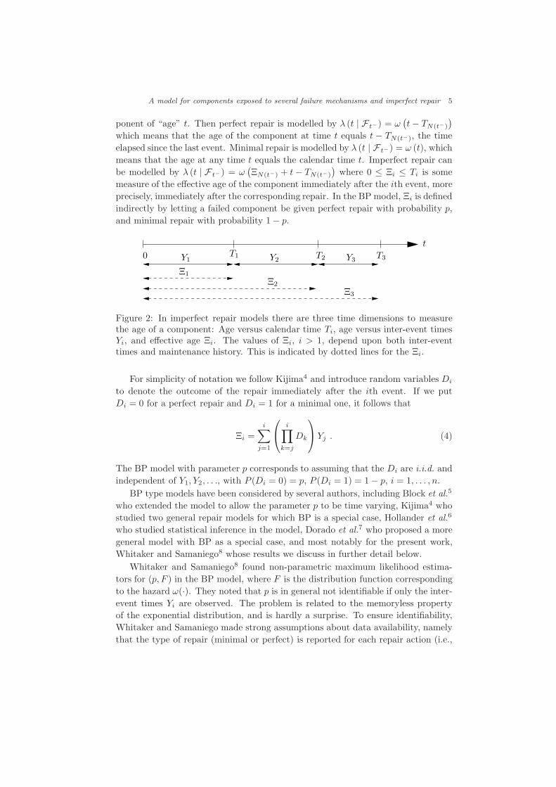
Figure 2: In imperfect repair models there are three time dimensions to measurethe age of a component: Age versus calendar time Ti, age versus inter-event timesYi, and effective age Ξi. The values of Ξi, i > 1, depend upon both inter-eventtimes and maintenance history. This is indicated by dotted lines for the Ξi.
For simplicity of notation we follow Kijima4 and introduce random variables Di
to denote the outcome of the repair immediately after the ith event. If we putDi = 0 for a perfect repair and Di = 1 for a minimal one, it follows that
Ξi =i∑
j=1
i∏
k=j
Dk
Yj . (4)
The BP model with parameter p corresponds to assuming that the Di are i.i.d. andindependent of Y1, Y2, . . ., with P (Di = 0) = p, P (Di = 1) = 1− p, i = 1, . . . , n.
BP type models have been considered by several authors, including Block et al.5
who extended the model to allow the parameter p to be time varying, Kijima4 whostudied two general repair models for which BP is a special case, Hollander et al.6
who studied statistical inference in the model, Dorado et al.7 who proposed a moregeneral model with BP as a special case, and most notably for the present work,Whitaker and Samaniego8 whose results we discuss in further detail below.
Whitaker and Samaniego8 found non-parametric maximum likelihood estima-tors for (p, F ) in the BP model, where F is the distribution function correspondingto the hazard ω(·). They noted that p is in general not identifiable if only the inter-event times Yi are observed. The problem is related to the memoryless propertyof the exponential distribution, and is hardly a surprise. To ensure identifiability,Whitaker and Samaniego made strong assumptions about data availability, namelythat the type of repair (minimal or perfect) is reported for each repair action (i.e.,
6 H. Langseth and B. H. Lindqvist
50 44 102 72 22 39 3 15197 188 79 88 46 5 5 3622 139 210 97 30 23 13 14
Table 2: Proschan’s air conditioner data; inter-event times of plane 7914.
the variables Dj are actually observed). In real applications, however, exact in-formation on the type of repair is rarely available. As we shall see in Section 4.2,identifiability of p is still possible in the model by appropriately modelling themaintenance actions.
In order to illustrate estimation in the BP model based on the Yi alone, weconsider the failure times of Plane 7914 from the air conditioner data of Proschan9
given in Table 2. These data were also used by Whitaker and Samaniego8. The jointdensity of the observations Y1, . . . , Yn can be calculated as a product of conditionaldensities,
f(y1, . . . , yn) = f(y1)f(y2|y1) · · · f(yn|y1, . . . , yn−1) .
For computation of the ith factor we condition on the unobserved D1, . . . , Di−1,getting
f(yi | y1, . . . , yi−1) =∑
d1,...,di−1
f(yi | y1, . . . , yi−1, d1, . . . , di−1)
× f(d1, . . . , di−1 | y1, . . . , yi−1)
=i∑
j=1
f(yi | y1, . . . , yi−1, dj−1 = 0, dj = · · · = di−1 = 1)
× P (Dj−1 = 0, Dj = · · · = Di−1 = 1)
=i∑
j=1
ω
i∑
k=j
yk
e
−[Ω(∑
i
k=jyk
)−Ω
(∑i−1
k=jyk
)](1− p)i−j pδ(j>1) ,
where Ω(x) =∫ x
0ω(t)dt is the cumulative hazard function and δ(j > 1) is 1 if j > 1
and 0 otherwise. The idea is to partition the set of vectors (d1, . . . , di−1) accordingto the number of 1s immediately preceding the ith event.
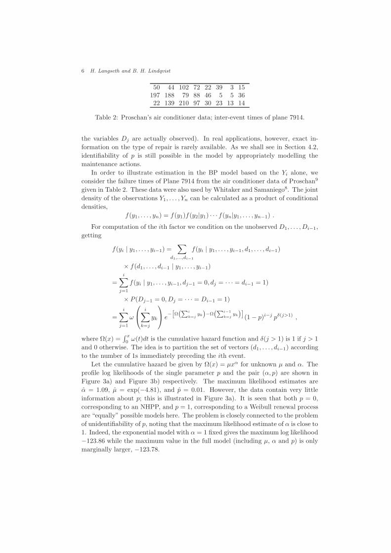
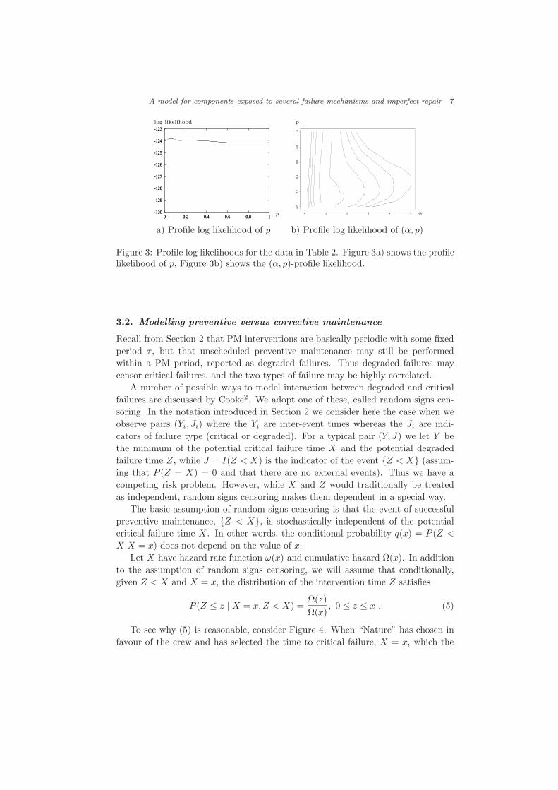
Let the cumulative hazard be given by Ω(x) = µxα for unknown µ and α. Theprofile log likelihoods of the single parameter p and the pair (α, p) are shown inFigure 3a) and Figure 3b) respectively. The maximum likelihood estimates areα = 1.09, µ = exp(−4.81), and p = 0.01. However, the data contain very littleinformation about p; this is illustrated in Figure 3a). It is seen that both p = 0,corresponding to an NHPP, and p = 1, corresponding to a Weibull renewal processare “equally” possible models here. The problem is closely connected to the problemof unidentifiability of p, noting that the maximum likelihood estimate of α is close to1. Indeed, the exponential model with α = 1 fixed gives the maximum log likelihood−123.86 while the maximum value in the full model (including µ, α and p) is onlymarginally larger, −123.78.
A model for components exposed to several failure mechanisms and imperfect repair 7
-130
-129
-128
-127
-126
-125
-124
-123
0 0.2 0.4 0.6 0.8 1-130
-129
-128
-127
-126
-125
-124
-123
0 0.2 0.4 0.6 0.8 1p
log likelihood
0 1 2 3 4 5
0.0
0.2
0.4
0.6
0.8
1.0
α
p
a) Profile log likelihood of p b) Profile log likelihood of (α, p)
Figure 3: Profile log likelihoods for the data in Table 2. Figure 3a) shows the profilelikelihood of p, Figure 3b) shows the (α, p)-profile likelihood.
3.2. Modelling preventive versus corrective maintenance
Recall from Section 2 that PM interventions are basically periodic with some fixedperiod τ , but that unscheduled preventive maintenance may still be performedwithin a PM period, reported as degraded failures. Thus degraded failures maycensor critical failures, and the two types of failure may be highly correlated.
A number of possible ways to model interaction between degraded and criticalfailures are discussed by Cooke2. We adopt one of these, called random signs cen-soring. In the notation introduced in Section 2 we consider here the case when weobserve pairs (Yi, Ji) where the Yi are inter-event times whereas the Ji are indi-cators of failure type (critical or degraded). For a typical pair (Y, J) we let Y bethe minimum of the potential critical failure time X and the potential degradedfailure time Z, while J = I(Z < X) is the indicator of the event Z < X (assum-ing that P (Z = X) = 0 and that there are no external events). Thus we have acompeting risk problem. However, while X and Z would traditionally be treatedas independent, random signs censoring makes them dependent in a special way.
The basic assumption of random signs censoring is that the event of successfulpreventive maintenance, Z < X, is stochastically independent of the potentialcritical failure time X . In other words, the conditional probability q(x) = P (Z <
X |X = x) does not depend on the value of x.Let X have hazard rate function ω(x) and cumulative hazard Ω(x). In addition
to the assumption of random signs censoring, we will assume that conditionally,given Z < X and X = x, the distribution of the intervention time Z satisfies
P (Z ≤ z | X = x, Z < X) =Ω(z)Ω(x)
, 0 ≤ z ≤ x . (5)
To see why (5) is reasonable, consider Figure 4. When “Nature” has chosen infavour of the crew and has selected the time to critical failure, X = x, which the

8 H. Langseth and B. H. Lindqvist
crew will have to beat, she first draws a value u uniformly from [0, Ω(x)]. Thenthe time for preventive maintenance is chosen as Z = Ω−1(u), where Ω−1(·) is theinverse function of Ω(·). Following this procedure makes the conditional densityof Z proportional to the intensity of the underlying failure process. This seemslike a coarse but somewhat reasonable description of the behaviour of a competentmaintenance crew.
t
Z X
Ω(t)
Ω(X)
u
Ω−1(u)
Figure 4: Time to PM conditioned on Z < X, X = x.
Our joint model for (X, Z) is thus defined from the following:
(i) X has hazard rate ω(·).
(ii) Z < X and X are stochastically independent.
(iii) Z given Z < X and X = x has distribution function (5).
These requirements determine the distribution of the observed pair (Y, J) asfollows. First, by (ii) we get
P (y ≤ Y ≤ y + dy, J = 0) = P (y ≤ X ≤ y + dy, X < Z)
= (1− q)ω(y) exp(−Ω(y)) dy
where we introduce the parameter q = P (Z < X). Next,
P (y ≤ Y ≤ y + dy, J = 1)
= P (y ≤ Z ≤ y + dy, Z < X)
=∫ ∞
y
P (y ≤ Z ≤ y + dy|X = x, Z < X)
× P (Z < X |X = x)ω(x) exp(−Ω(x)) dx
= q ω(y) dy
∫ ∞
y
ω(x) exp(−Ω(x)) / Ω(x) dx
= q ω(y) Ie(Ω(y)) dy ,
where Ie(t) =∫ ∞
texp(−u)/u du is known as the exponential integral10.

A model for components exposed to several failure mechanisms and imperfect repair 9
It is now straightforward to establish the density and distribution function of Y ,
fY (y) = (1− q) ω(y) exp (−Ω(y)) + q ω(y) Ie(Ω(y)) (6)
andFY (y) = P (Y ≤ y) = 1− exp(−Ω(y)) + q Ω(y) Ie(Ω(y)) . (7)
Note that the proposed maintenance model introduces only one new parameter,namely q. We can interpret this parameter in terms of the alertness of the mainte-nance crew; a large value of q corresponds to a crew that is able to prevent a largepart of the critical failures.
The distribution (6) for Y is a mixture distribution, with one component repre-senting the failure distribution one would have without preventive maintenance, andthe other mixture component being the conditional density of time for PM giventhat PM “beats” critical failure. It is worth noticing that the distribution withdensity ω(y) Ie(Ω(y)) is stochastically smaller than the distribution with densityω(y) exp(−Ω(y)); this is a general consequence of random signs censoring.
4. General model
Recall that the events in our most general setting are either critical failures, de-graded failures or external events; consider Figure 2. We shall assume that correc-tive maintenance is always performed following a critical failure, while preventivemaintenance is performed both after degraded failures and external events. More-over, in the case of several failure mechanisms, any failure is treated as an externalevent for all failure mechanisms except the one failing.
4.1. Single failure mechanism
In this case the data for one component are (Yi, Ji); i = 1, . . . , n with Ji now definedas in (2) with three possible values. Suppose for a moment that all repairs, bothcorrective and preventive, are perfect. Then we shall assume that the (Yi, Ji) arei.i.d. observations of (Y, J) where Y = min(X, Z, U), (X, Z) is distributed as inSection 3.2, and U is the (potential) time of an external event. The U is assumedto be stochastically independent of (X, Z) and to have a distribution which doesnot depend on the parameters of our model. It follows that we can disregard theterms corresponding to U in the likelihood calculation. The likelihood contributionfrom an observation (Y, J) will therefore be as follows (see Section 3.2):
f(y, 0) = (1− q)ω(y) exp (−Ω(y))
f(y, 1) = q ω(y) Ie(Ω(y)) (8)
f(y, 2) = exp (−Ω(y))− q Ω(y) Ie(Ω(y)) .
The last expression follows from (7) and corresponds to the case where all we knowis that max(X, Z) > y.
To the model given above we now add imperfect repair. Recall that in the BPmodel there is a probability p of perfect repair (Di = 0) after each event. We shall
10 H. Langseth and B. H. Lindqvist
here distinguish between preventive maintenance and corrective maintenance by let-ting Di equal 0 with probability p if the ith event is a preventive maintenance or anexternal event, and with probability π if the ith event is a critical failure. Moreover,we shall assume that for all i we have D1, . . . , Di conditionally independent giveny1, . . . , yi, j1, . . . , ji.
From this we are able to write down the likelihood of the data as a product of thefollowing conditional distributions. The derivation is a straightforward extension ofthe one in Section 3.1.
f((yi, ji) | (y1, j1), . . . , (yi−1, ji−1)
)=
∑d1,...,di−1
f((yi, ji) | (y1, j1), . . . , (yi−1, ji−1), d1, . . . , di−1)
× f(d1, . . . , di−1|(y1, j1), . . . , (yi−1, ji−1))
=i∑
j=1
f
(yi, ji)
∣∣∣∣∣∣ξi−1 =i−1∑k=j
yk
× P (Dj−1 = 0, Dj = · · · = Di−1 = 1|j1, . . . , ji−1) .
Here P (Dj−1 = 0, Dj = · · · = Di−1 = 1 | j1, . . . , ji−1) is a simple function of p andπ. Thus, what remains to be defined are the conditional densities f ((yi, ji)|ξi−1), i.e.the conditional densities of (Yi, Ji) given that the age of the component immediatelyafter the (i − 1)th event is ξi−1. We shall define these to equal the conditionaldensities given no event in (0, ξi−1), of the distribution given in (8). Thus we have
f ((yi, 0) | ξi−1) =(1− q)ω(ξi−1 + yi) exp(−(Ω(ξi−1 + yi)))
exp(−Ω(ξi−1))− q Ω(ξi−1) Ie(Ω(ξi−1))
f ((yi, 1) | ξi−1) =q ω(ξi−1 + yi) Ie(Ω(ξi−1 + yi))
exp(−Ω(ξi−1))− q Ω(ξi−1) Ie(Ω(ξi−1))
f ((yi, 2) | ξi−1) =exp(−Ω(ξi−1 + yi))− q Ω(ξi−1 + yi) Ie(Ω(ξi−1 + yi))
exp(−Ω(ξi−1))− q Ω(ξi−1) Ie(Ω(ξi−1)).
If we have data from several independent components, the complete likelihoodis given as the product of the individual likelihoods.
The model for a single failure mechanism is displayed as a directed acyclicgraph11,12 in Figure 5. Due to the imperfect repair we do not have guaranteedrenewals at each event, hence we have to use a time evolving model to capture thedynamics in the system. For clarity, only time-slice r (i.e., the time between eventr − 1 and r) is shown.
4.2. Identifiability of parameters
The present discussion of identifiability is inspired by the corresponding discussionby Whitaker and Samaniego8, who considered the simple BP model.
Refer again to the model of the previous subsection. We assume here that,conditional on (Y1, J1), (Y2, J2), . . . , (Yi−1, Ji−1), the (potential) time to the next

A model for components exposed to several failure mechanisms and imperfect repair 11
Ξr−1
Zr
Xr Yr Ξr
Jr
Figure 5: The model for a single failure mechanism, when only time-slice r is shown.The double-lined nodes represent the observable variables. Ξr is the effective ageimmediately after the rth repair, Ξr depends on Ξr−1 together with what happensduring the rth time-slice. Xr is the potential time to critical failure (given thehistory), and Zr is the corresponding potential time to a degraded failure. Yr is therth inter-event time, and Jr = I(Zr < Xr).
external event is a random variable U with continuous distribution G and supporton all of (0, τ ] where τ as before is the regular maintenance interval. Moreover, thedistribution G does not depend on the parameters of the model, and it is kept fixedin the following.
We also assume that ω(x) > 0 for all x > 0 and that 0 < q < 1. The parametersof the model are ω, q, p, π. These, together with G, determine a distribution of(Y1, J1), . . . , (Yn, Jn) which we call F(ω,q,p,π). Here n is kept fixed.
The question of identifiability can be put as follows: Suppose
F(ω,q,p,π) = F(ω∗,q∗,p∗,π∗) , (9)
which means that the two parameterizations lead to the same distribution of theobservations (Y1, J1), . . . , (Yn, Jn). Can we from this conclude that ω = ω∗, q = q∗,p = p∗, π = π∗?
First note that (9) implies that the distribution of (Y1, J1) is the same underthe two parameterizations; Y1 = min(X, Z, U). It is clear that each of the followingtwo types of probabilities are the same under the two parameterizations,
P (x ≤ X ≤ x + dx, Z > x, U > x)
P (z ≤ Z ≤ z + dz, X > z, U > z).
By independence of (X, Z) and U , and since P (U > x) > 0 if and only if x < τ , weconclude that each of the following two types of probabilities are equal under thetwo parameterizations,
P (x ≤ X ≤ x + dx, Z > x); x < τ
P (z ≤ Z ≤ z + dz, X > z); z < τ.
These probabilities can be written respectively
(1− q)ω(x) e−Ω(x) dx; x < τ
q ω(z) Ie(Ω(z)) dz; z < τ .

12 H. Langseth and B. H. Lindqvist
Thus, by integrating from 0 to x we conclude that (9) implies for x ≤ τ
(1− q)(1− e−Ω(x)
)= (1− q∗)
(1− e−Ω∗(x)
)(10)
q(1− e−Ω(x) + Ω(x)Ie(Ω(x))
)= q∗
(1− e−Ω∗(x) + Ω∗(x)Ie(Ω∗(x))
). (11)
We shall now see that this implies that q = q∗ and Ω(x) = Ω∗(x) for all x ≤ τ .Suppose, for contradiction, that there is an x0 ≤ τ such that Ω(x0) < Ω∗(x0). Thensince both 1−exp(−t) and 1−exp(−t)+ t Ie(t) are strictly increasing in t, it followsfrom respectively (10) and (11) that 1 − q > 1 − q∗ and q > q∗. But this is acontradiction. In the same manner we get a contradiction if Ω(x0) > Ω∗(x0). ThusΩ(x) = Ω∗(x) for all x ≤ τ (so ω(x) = ω∗(x) for all x ≤ τ) and hence also q = q∗.
We shall see below that in fact we have Ω(x) = Ω∗(x) on the interval (0, nτ),but first we shall consider the identifiability of p and π. For this end we consider thejoint distribution of (Y1, J1), (Y2, J2). In the same way as already demonstrated wecan disregard U in the discussion, by independence, but we need to restrict y1, y2
so that y1 + y2 ≤ τ . First, look at
P(y1 ≤ Y1 ≤ y1 + dy1, J1 = 0, y2 ≤ Y2 ≤ y2 + dy2, J2 = 0
)(12)
= (1− q)ω(y1) e−Ω(y1)[π(1 − q)ω(y2)e−Ω(y2)
+(1− π) (1− q)ω(y1 + y2) exp(−Ω(y1 + y2))
exp(−Ω(y1))− q Ω(y1) Ie(Ω(y1))
]dy1 dy2 .
This is a linear function of π with coefficient of π proportional to
ω(y2) exp(−Ω(y2))− ω(y1 + y2) exp(−Ω(y1 + y2))exp(−Ω(y1))− q Ω(y1) Ie(Ω(y1))
. (13)
Using the assumption that 0 < q < 1 we thus conclude that π = π∗ unless (13)equals 0 for all y1 and y2 with y1+y2 ≤ τ . Making the similar computation, puttingJ2 = 1 instead of J2 = 0 in (12), we can similarly conclude that π = π∗ unless
ω(y2)Ie(Ω(y2))− ω(y1 + y2) Ie(Ω(y1 + y2))exp(−Ω(y1))− q Ω(y1) Ie(Ω(y1))
(14)
equals 0 for all y1 and y2 with y1 + y2 ≤ τ . Now, if both (13) and (14) were 0 forall y1 and y2 with y1 + y2 ≤ τ , then we would necessarily have
exp(−Ω(y2))Ie(Ω(y2))
=exp(−Ω(y1 + y2))
Ie(Ω(y1 + y2))(15)
for all y1 and y2 with y1 + y2 ≤ τ . Since we have assumed that ω(·) is strictlypositive, (15) would imply that exp(−t)/Ie(t) is constant for t in some interval(a, b). This is of course impossible by the definition of Ie(·), and it follows that notboth of (13) and (14) can be identically zero. Hence π is identifiable.
Identifiability of p is concluded in the same way by putting J1 = 1 instead ofJ1 = 0 in (12).

A model for components exposed to several failure mechanisms and imperfect repair 13
So far we have concluded equality of the parameters q, p, π under the two pa-rameterizations, while we have concluded that Ω(x) = Ω∗(x) for all x ≤ τ . Butthen, putting y1 = τ in (12), while letting y2 run from 0 to τ , it follows thatΩ(x) = Ω∗(x) also for all τ < x ≤ 2τ . By continuing we can eventually concludethat Ω(x) = Ω∗(x) for all 0 < x ≤ nτ .
If τ =∞, then of course the whole function ω(·) is identifiable. However, even ifτ <∞ we may have identifiability of all of ω(·). For example, suppose Ω(x) = µxα
with µ, α positive parameters. Then the parameters are identifiable since (10) inthis case implies that
µxα = µ∗xα∗
for all x ≤ τ . This clearly implies the pairwise equality of the parameters.
4.3. Several failure mechanisms
We now look at how to extend the model of Section 4.2 to k > 1 failure mechanismsand data given as in (1) or (3).
Our basic assumption is that the different failure mechanisms M1, . . . , Mk actindependently on the component. More precisely we let the complete likelihoodfor the data be given as the product of the likelihoods for each failure mechanism.Note that the set of events is the same for all failure mechanisms, and that failuredue to one failure mechanism is treated as an external event for the other failuremechanisms.
The above assumption implies a kind of independence of the maintenance foreach failure mechanism. Essentially we assume that the pairs (X, Z) are indepen-dent across failure mechanisms. This is appropriate if there are different mainte-nance crews connected to each failure mechanisms, or could otherwise mean thatthe “signals” of degradation emitted from the component are independent acrossfailure mechanisms.
Another way of interpreting our assumption is that, conditional on
(y1, k1, j1), . . . , (yi−1, ki−1, ji−1)
the next vector (Yi, Ki, Ji) corresponds to a competing risk situation involving m
independent risks, one for each failure mechanism, and each with properties as forthe model given in Section 4.1.
The parameters (ω, q, p, π) may (and will) in general depend on the failure mech-anism. As regards identifiability of parameters, this will follow from the results forsingle failure mechanisms of Section 4.2 by the assumed independence of failuremechanisms.
If we have data from several independent components of the same kind, givenas in (3), then the complete likelihood is given as the product of the likelihoods foreach component.
Figure 6 depicts the complete model for time-slice r represented by a directedacyclic graph, confer also Figure 5.

14 H. Langseth and B. H. Lindqvist
..
.
Ξkr
Ξ1r
..
.
Ξkr−1
Ξ1r−1
Y kr
Jkr
Xkr
Zkr
Yr
Jr
Z1r
X1r
J1r
Y 1r
Figure 6: The complete model, but only showing time-slice r. The random variablesare given a subscript index indicating the time-slice, and a superscript index showingthe failure mechanism. For example, Ξm
r is the effective age of the m’th failuremechanism immediately after the r’th event. Only nodes drawn with double-lineare observed.
Deformation Leakage Breakage Other# Critical failures 4 1 1 2# Degraded failures 8 2 0 4
Table 3: Number of failures per failure mechanism.
5. Parameter estimation
5.1. Calculation scheme
The complete model as described in Section 4 involves some important conditionalindependence properties that both special purpose maximum-likelihood estimatoralgorithms as well as Markov Chain Monte Carlo simulations can benefit from. Inthis section we have used maximum likelihood methods.
5.2. A case study
To exemplify the merits of the proposed model, we use Phase IV of the Gas Turbinedataset from the Offshore Reliability Database13. Only the Gas Generator subsys-tem is included in the study. We analyse data from a single offshore installationto ensure maximum homogeneity of the data sample. The dataset consists of 23mechanical components, which are followed over a total of 603.690 operating hours.There are 22 failures, out of which 8 are classified as critical and 14 as degraded. Thefailures are distributed over four different failure mechanisms (so k = 4), namelydeformation, leakage, breakage and other mechanical failure.

A model for components exposed to several failure mechanisms and imperfect repair 15
Deformation Leakage Breakage OtherHazard (µm) 2.5 · 10−6 1.3 · 10−5 8.3 · 10−7 5.6 · 10−6
Preventive maint. (pm) 0.6 0.3 1.0 0.8Corrective maint. (pκ
m) 1.0 1.0 1.0 1.0
Table 4: Estimated hazard rate and probability of successful maintenance.
Deformation Leakage Breakage OtherMTTFFNaked 4.0 · 105 7.7 · 104 1.2 · 106 1.8 · 105MTTFFOFR 6.0 · 105 1.5 · 105 6.0 · 105 3.0 · 105
Table 5: Estimated MTTFF in our model and the “observed failure rate” model.
The PM history for the gas turbines consists of 78 PM events. The PM intervals(“τ”) for the different components vary between 8 and 12 calendar months.
5.3. Results
The data can be put on the form (3) so the complete likelihood can be calculatedas described in Section 4. Having a small number of critical failures, the estimatesof π1, . . . , π4 will not be reliable; the number of critical failures is simply too small.To reduce the number of parameters we introduce κ > 0 defined so that πm = pκ
m
for m = 1, . . . , 4. Here κ indicates the difference between the effect of preventiveand corrective maintenance. A small value of κ means that corrective maintenanceis much more beneficial than the preventive, and a value close to 1 judges the twomaintenance operations about equal. In the same way, we assume that q1 = · · · = q4,and use q to denote these variables.
We also use a simple parametric forms of the ωi(·), namely the constant haz-ards ωi(t) = µi, i = 1, . . . , 4. The results of maximum likelihood estimation arepresented in Table 4. The estimated value of q is q = .4, while κ = 1 · 10−2. Thelatter value indicates that corrective maintenance actions are highly effective.
It is also interesting to calculate the mean time to first failure (MTTFF ) hadthere been no maintenance. This value, which we name MTTFFNaked, shows thenature of the underlying failure process unbiased by the maintenance regime; itcan be estimated directly by 1/µi in the present setting. In Table 5 we compareMTTFFNaked to the “observed failure rate” estimators given by
MTTFFOFR =#Total Operating Time
#Critical Failures
to see the effect of including maintenance in the model.It is worth noticing that the OFR-estimates are inclined to be more optimistic
than the estimators from our model. This is because degraded failures tend tocensor potential critical failures, and this influences the OFR-estimate.

16 H. Langseth and B. H. Lindqvist
6. Concluding remarks
In this paper we have proposed a simple but flexible model for maintained compo-nents which are subject to a variety of failure mechanisms. The proposed modelhas the standard models of perfect and minimal repair as special cases. Moreover,some of the parameters we estimate (namely pm, πm and qm) can be used to ex-amine the sufficiency of these smaller models. “Small” values of qm accompaniedby “extreme” values of all pm and πm (either “close” to one or zero) indicate thatreduced models are detailed enough to capture the main effects in the data. Mak-ing specific model assumptions regarding the preventive maintenance we are ableto prove identifiability of all parameters.
We note that many models simpler than ours may be useful if explicit notionof maintenance quality is considered unimportant14,15,16. In our experience, themodel of Lawless and Thiagarajah17,
λ(t | F t−) = exp(α + β g1(t) + γ g2(t− TN(t−)
), (16)
where α, β and γ are unknown parameters, and g1 and g2 are known functions,offers good predictive ability in the setting corresponding to Section 3.2. Observethat the conditional intensity in (16) depends both on the age t and the time sincelast failure t − TN(t−); hence it can be considered to be an imperfect repair modelwith perfect and minimal repair as special cases. However, the model is difficult tointerpret with respect to the physical meaning of the parameters, and is thereforenot satisfactory in our more general setting. Our motivation has been to build amodel that could be used to estimate the effect of maintenance, where “effect” hasbeen connected to the model parameters qm, pm and πm. Here qm is indicative ofthe crew’s eagerness, their ability to perform maintenance at the correct times to tryto stop evolving failures. The pm and πm indicate the crew’s thoroughness; theirability to actually stop the failure development. The proposed model indirectlyestimates the naked failure rate, and on a specific case using real life data theseestimates are significantly different from those found by “traditional” models.
We make modest demands regarding data availability: Only the inter-failuretimes and the failure mechanisms leading to the failure accompanied by the pre-ventive maintenance program are required. This information is available in mostmodern reliability data banks.
Acknowledgements
We would like to thank Tim J. Bedford for an interesting conversation about themodel for PM versus critical failures and Roger M. Cooke for discussions regard-ing the applicability of random signs censoring with respect to the OREDA data.Previous short versions of this manuscript18,19 were presented at the conferencesESREL‘99 and MMR‘02. The first author was supported by a grant from the Re-search Council of Norway.

A model for components exposed to several failure mechanisms and imperfect repair 17
References
1. M. Brown and F. Proschan. Imperfect repair. Journal of Applied Probability, 20:851–859, 1983.
2. R. M. Cooke. The design of reliability data bases, Part I and Part II. ReliabilityEngineering and System Safety, 52:137–146 and 209–223, 1996.
3. P. Andersen, Ø. Borgan, R. Gill, and N. Keiding. Statistical models based on countingprocesses. Springer, New York, 1992.
4. M. Kijima. Some results for repairable systems with general repair. Journal of AppliedProbability, 26:89–102, 1989.
5. H. Block, W. Borges, and T. Savits. Age dependent minimal repair. Journal of AppliedProbability, 22:370–385, 1985.
6. M. Hollander, B. Presnell, and J. Sethuraman. Nonparametric methods for imperfectrepair models. Annals of Statistics, 20:879–896, 1992.
7. C. Dorado, M. Hollander, and J. Sethuraman. Nonparametric estimation for a generalrepair model. Annals of Statistics, 25:1140–1160, 1997.
8. L. R. Whitaker and F. J. Samaniego. Estimating the reliability of systems subject toimperfect repair. Journal of American Statistical Association, 84:301–309, 1989.
9. F. Proschan. Theoretical explanation of observed decreasing failure rate. Technomet-rics, 5:375–383, 1963.
10. M. Abramowitz and I. A. Stegun. Handbook of Mathematical Functions. DoverPubl., New York, 1965.
11. J. Pearl. Probabilistic Reasoning in Intelligent Systems: Networks of PlausibleInference. Morgan Kaufmann Publishers, San Mateo, CA., 1988.
12. F. V. Jensen. Bayesian Networks and Decision Graphs. Springer Verlag, New York,2001.
13. OREDA. Offshore Reliability Data. Distributed by Det Norske Veritas, P.O. Box300, N-1322 Høvik, 3rd edition, 1997.
14. H. Pham and H. Wang. Multivariate imperfect repair. European Journal of Opera-tions Research, 94:425–428, 1996.
15. P. A. Akersten. Imperfect repair models. In S. Lydersen, G. K. Hansen, and H. A.Sandtorv, editors, Proceedings of the ninth European Conference on Safety andReliability – ESREL’98, pages 369–372, Rotterdam, 1998. A. A. Balkema.
16. B. H. Lindqvist. Repairable systems with general repair. In G. I. Schueller and P. Kafka,editors, Proceedings of the tenth European Conference on Safety and Reliability– ESREL’99, pages 43–48, Munchen, Germany, 1999. A. A. Balkema.
17. J. F. Lawless and K. Thiagarajah. A point process model incorporating renewals andtime trends, with applications to repairable systems. Technometrics, 38:131–138, 1996.
18. H. Langseth. Modelling maintenance for components under competing risk. In G. I.Schueller and P. Kafka, editors, Proceedings of the tenth European Conference onSafety and Reliability – ESREL’99, pages 179–184, Munchen, Germany, 1999. A. A.Balkema.
19. H. Langseth and B. H. Lindqvist. Modelling imperfect maintenance and repair ofcomponents under competing risk. In H. Langseth and B. H. Lindqvist, editors, Com-munuications of the Third International Conference on Mathematical Methodsin Reliability – Methodology and Practice, page 359, Trondheim, Norway, 2002.


II
Decision Theoretic Troubleshooting of Coherent Systems


Decision Theoretic Troubleshooting of
Coherent Systems
Helge Langseth 1 and Finn V. Jensen
Department of Computer Science, Aalborg University, Fredrik Bajers Vej 7E,DK-9220 Aalborg Ø, Denmark
Abstract
We present an approach to efficiently generating an inspection strategy for faultdiagnosis. We extend the traditional troubleshooting framework to model non-perfect repair actions, and we include questions. Questions are troubleshooting stepsthat do not aim at repairing the device, but merely are performed to capture infor-mation about the failed equipment, and thereby ease the identification and repairof the fault. We show how Vesely and Fussell’s measure of component importanceextends to this situation, and focus on its applicability to compare troubleshootingsteps. We give an approximate algorithm for generating a “good” troubleshootingstrategy in cases where the assumptions underlying Vesely and Fussell’s componentimportance are violated, and discuss how to incorporate questions into this trou-bleshooting strategy. Finally, we utilize certain properties of the domain to proposea fast calculation scheme.
Key words: Repair strategies, Bayesian networks, fault diagnosis, Vesely andFussell component importance.
Email addresses: [email protected] (Helge Langseth), [email protected](Finn V. Jensen).1 Current affiliation: Department of Mathematical Sciences, Norwegian Universityof Science and Technology, N-7491 Trondheim, Norway.
To appear in Reliability Engineering and System Safety

1 Introduction
This paper describes a troubleshooting system which has been developed inthe SACSO 2 project, and which is partly implemented in the BATS 3 tool.This is a troubleshooting (TS) system for performing efficient troubleshootingof electro-mechanical equipment, and it is currently employed in the printerdomain. It is important to notice that the BATS tool is created to offer printerusers a web-based interface to a decision-theoretic TS-system; it is not in-tended exclusively for maintenance personnel who are trained to handle theequipment that is to be repaired. The goal is that any user, however inexpe-rienced, should be able to repair the failed equipment on his own instead ofrelying on professional help. By design the TS-system we describe thereforediffers from other TS-systems (see e.g. [1–7]) in several aspects. Most impor-tantly the users of the TS-system may be inexperienced with handling andrepairing the failed equipment. Hence, they may fail to repair broken com-ponents, e.g., by seating a new network card incorrectly. Furthermore, thismay even happen without the user realizing the mistake. It is therefore cru-cial for the TS-system to explicitly include the possibility that users performprescribed repair actions incorrectly in the TS-model.
Secondly, the users are expected to have limited knowledge about (and interestin) the design of the malfunctioning equipment. They cannot be expected tobe interested in finding the cause of a problem; they merely want to repairit. Focusing on the identification of the faulty minimal cutset, as in [4–7],is therefore not expected to be relevant for the foreseen group of users. Thetroubleshooting will thus be terminated as soon as the equipment is repaired;that is, we assume that the user is satisfied with a minimal repair of the failedequipment. Perfect repair is not necessarily accomplished by using our TS-system (and not by the methods in [4–7] either), but may be considered usingother means.
Finally, as the faulty device can be located under a variety of external con-ditions, the TS-system can pose questions to the user in order to survey thefaulty equipment’s surroundings. Although these questions initially increasethe cost of the troubleshooting, they may shed light on the situation, andultimately decrease the overall cost of repairing the equipment.
To formalize, let the faulty equipment consist of K components X = X1, . . . ,XK. Each component is either faulty (Xi = faulty) or operating (Xi = ok),and as the status of each component is unknown to the TS-system when the
2 The SACSO (Systems for Automated Customer Support Operations) projectconstitutes joint work between the Research Unit for Decision Support Systems atAalborg University and Customer Support R&D at Hewlett-Packard.3 BATS (Bayesian Automated Troubleshooting System) is available from Dezideover the internet: http://www.dezide.dk/.
2

troubleshooting starts, X is considered a set of random variables. The equip-ment consists of R Minimal Cut Sets (MCSs), and we use C = C1, . . . , CRfor the collection of these. A MCS is faulty (Ci = faulty) if all its members arefaulty. Otherwise it is operating (Ci = ok). The equipment is assumed to befaulty at the time when troubleshooting starts; troubleshooting is terminatedas soon as the equipment is brought back to operating modus. We will assumethat only one MCS is in its faulty state, and use CF to denote the faultyMCS (named the actual MCS in [4]). This assumption is common for mostTS-systems, and it is usually justified by considering systems that are usedalmost continuously, and thus (like a printer) tested frequently. It is unlikelythat several components should fail approximately simultaneously. Commoncause failures (due to, e.g., stroke of lightning, pouring coffee into the printer,etc.) are easily detected, and are handled separately. Note that if more thanone MCS is faulty the proposed method will still repair the equipment, al-though not necessarily in an optimal fashion. 4 The TS-system may choosefrom a set of N possible actions and will ask the user to perform (some of)them to remedy the problem. The outcome of the actions are modelled by aset of random variables A = A1, . . . , AN in the TS-system. There are alsoM predefined questions that the TS-system may pose to the user; the answersto these questions are modelled by the random variables Q = Q1, . . . , QM.Since there is a one-to-one mapping between actions the TS-system can askthe user to perform and the random variables in the set A, we will refer toA as the set of actions and say “perform A ∈ A” when we really mean thatthe action associated with A is executed. In the same manner we call Q thequestions, and use the term “pose the question Q ∈ Q” when strictly speakinga question is posed, and the random variable Q models the answer to thatquestion. A TS-step is a step in a TS-strategy, either a repair step (termedaction) or an information-gathering step (termed question). To each TS-stepBi the associated cost is denoted by Ci. The system is informed about theoutcome of each TS-step after it has been performed (i.e., the state of theassociated random variable is observed).
The goal of a TS-system is to provide a “good” TS-strategy. Formally, a TS-strategy S is an ordering of TS-steps, such that new TS-steps are prescribeduntil the equipment is repaired or all steps have been performed. The orderingof steps may depend on the outcome of the steps already performed in the
4 Srinivas [8] presents a modified algorithm to handle troubleshooting in serialsystems where more than one component (and hence more than one MCS) maybe faulty; it turns out that optimal troubleshooting in this case requires a balancebetween cost and probability of successful repair that is different from what isoptimal in our situation. When presented with a system where more than one MCSis in its faulty state, our system may thus perform sub-optimally: The user may beasked to perform the repair in a way more expensive than had been required if wehad not made this assumption.
3

strategy (there is for instance no need to examine the network connection ifthe printer test-page is printed correctly). Any TS-strategy can be representedby a strategy tree, see Fig. 1 for an example. The internal nodes in the strategytree (depicted as ovals) represent chance nodes; TS-steps that we do not knowthe outcome of initially. Each possible outcome of a chance node correspondsto a unique sub-tree in the strategy tree, which is found by selecting the edgelabelled with that particular outcome. The TS-strategy depicted in Fig. 1starts by posing QS , and if the answer is QS = yes, the TS-strategy prescribesto perform action A2; if QS = no, then the question QK should be posed.The terminal nodes (depicted as diamonds) signify that the troubleshootingstrategy has ended, either because the problem is solved or because the setof actions has been exhausted. Note that this is a simple example, where weassume only two possible answers (yes and no) to the questions QS and QK .
QS
A2 A4 A3 A1 A5
A4 A2 A5 A1
A5 A1 A4 A3 A2
j
q
ok ok ok ok ok
ok ok ok ok okok ok ok ok
ok ok ok ok ok
A3
yes
a b c d e
f g h i
k l n o
QK
yes
no
no
p
rno no no no no
no no no nono
no no no no no
m
Fig. 1. A TS-strategy represented by a strategy tree; A = A1, . . . , A5 andQ = QS , QK.
How “good” a TS-strategy is, is judged by its expected cost of repair, ECR,which is a function of the Ci. This is in accordance with the decision-theoreticformulation of the troubleshooting task: One should balance the cost of a TS-step with the likelihood of the step to be beneficial, so that the optimal TS-strategy can be found [3]. Breese and Heckerman [9] used Bayesian networksto model the troubleshooting domain, and Jensen et al. [10] report extensionsto that framework. In [9,10] the domains under study were restricted to beserial systems, i.e., systems where all cutsets were singletons. In this paper wewill extend these frameworks to work with any coherent system (representedby its cutsets). Finding the strategy which minimizes the ECR is NP-hard ingeneral [11], so we our goal will be to approximate the optimal strategy.
The printer industry spends millions of dollars every year on customers sup-port; mainly to provide telephone-support and on-site troubleshooting. Thishas sparked an interest for building automated troubleshooting systems which
4

can resolve some of the printer users’ problems without requiring support fromcall agents. A printing system consists of several components: The applicationfrom which the printing command is sent, the printer driver, the network con-nection, the server controlling the printer, the printer itself, etc. It typicallyhas about 40 different failure-modes, e.g., Light print. Each failure-mode canbe caused by several component failures, and we have one TS-system for eachof them. 5 The typical size of these TS-models is about 30 actions and 15questions. We will not describe the printer model in further detail, as the TS-system we propose is general in nature; the interested reader is referred to[10,12].
The rest of the paper is outlined as follows: In Section 2 we describe thebasic system model, and the formal language used to describe it. Section 3 isdevoted to how the TS-system sequences actions, and handling of questionsare described in Section 4. The calculation scheme is described in detail inSection 5, and we conclude in Section 6.
2 The troubleshooting model
In this section we will describe the troubleshooting model, and in partic-ular focus on the modelling assumptions that we make. To do so, we startby introducing Bayesian networks (BNs), which constitute the representationlanguage we employ. We then give a detailed description of how we generatea BN-representation of the troubleshooting domain.
2.1 Bayesian networks
Our system represents the TS-domain by a Bayesian network [13,14]. BNshave a long history of usage in the reliability and safety sciences, ranging fromthe early works [15,16] to the more recent contributions, see, e.g., [8–12,17–20]. BNs offer a flexible language to describe the TS-model, and we utilizethis to make a realistic model of the interactions one can have with the failedequipment; specifically we can define repair steps including non-perfect repair,as well as information-gathering steps.
A Bayesian network over the discrete random variables X is a compact rep-resentation of the probability mass function P (X = x). A BN consists ofa qualitative part; a directed acyclic graph, and a quantitative part; a set ofconditional probability tables. More formally, a Bayesian network representingthe probability mass function of a stochastic vector X is a 2-tuple
(G,ΘG
).
G is a directed acyclic graph G = (V, E), where V is the set of nodes in thegraph and E is the set of directed edges. There is a bijection between X and
5 The first information the user enters into the system is the failure-mode he wantsto troubleshoot. If some failure-modes are not easily distinguishable we have joinedthem into one TS-model.
5
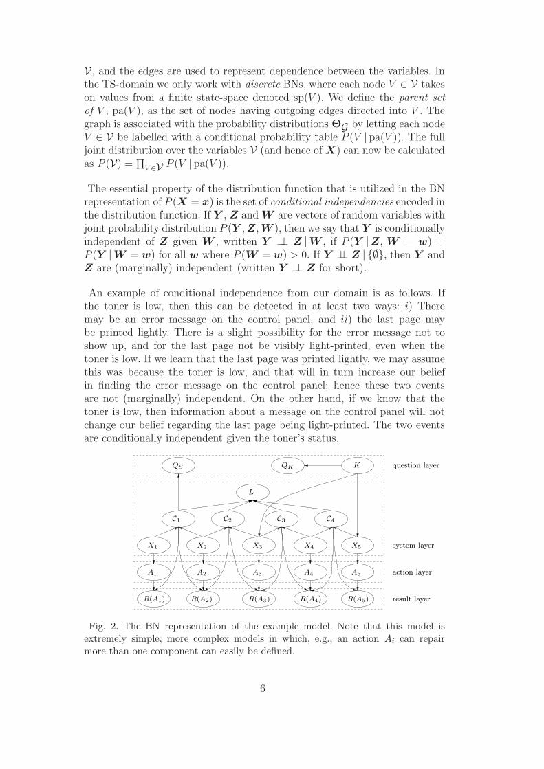
V, and the edges are used to represent dependence between the variables. Inthe TS-domain we only work with discrete BNs, where each node V ∈ V takeson values from a finite state-space denoted sp(V ). We define the parent setof V , pa(V ), as the set of nodes having outgoing edges directed into V . Thegraph is associated with the probability distributions ΘG by letting each nodeV ∈ V be labelled with a conditional probability table P (V | pa(V )). The fulljoint distribution over the variables V (and hence of X) can now be calculatedas P (V) =
∏V ∈V P (V | pa(V )).
The essential property of the distribution function that is utilized in the BNrepresentation of P (X = x) is the set of conditional independencies encoded inthe distribution function: If Y , Z and W are vectors of random variables withjoint probability distribution P (Y , Z, W ), then we say that Y is conditionallyindependent of Z given W , written Y ⊥⊥ Z |W , if P (Y |Z, W = w) =P (Y |W = w) for all w where P (W = w) > 0. If Y ⊥⊥ Z | ∅, then Y andZ are (marginally) independent (written Y ⊥⊥ Z for short).
An example of conditional independence from our domain is as follows. Ifthe toner is low, then this can be detected in at least two ways: i) Theremay be an error message on the control panel, and ii) the last page maybe printed lightly. There is a slight possibility for the error message not toshow up, and for the last page not be visibly light-printed, even when thetoner is low. If we learn that the last page was printed lightly, we may assumethis was because the toner is low, and that will in turn increase our beliefin finding the error message on the control panel; hence these two eventsare not (marginally) independent. On the other hand, if we know that thetoner is low, then information about a message on the control panel will notchange our belief regarding the last page being light-printed. The two eventsare conditionally independent given the toner’s status.
X2
L
K
C1 C3C2 C4
X1 X3 X5
A4A3A1 A5
R(A1) R(A2) R(A3) R(A4) R(A5)
X4
QS
A2
QK question layer
system layer
action layer
result layer
Fig. 2. The BN representation of the example model. Note that this model isextremely simple; more complex models in which, e.g., an action Ai can repairmore than one component can easily be defined.
6

2.2 The basic troubleshooting model
The faulty equipment and the effect of interactions between the repair per-sonnel and this equipment are modelled in a BN. As our starting point we usea BN model of the system generated from the MCS representation (see [20] forhow this translation can be done). This part of the BN is denoted the systemlayer in Fig. 2; the system layer is the part of the BN that mimics the faulttree in Fig. 3. Note that we have introduced a constraint node 6 L to enforcethe assumption that exactly one MCS is in its faulty state. All calculationsare performed conditional on this assumption, and we will for simplicity ofexposition not mention this conditioning explicitly in the following. Next, theMCSs are modelled by logical functions, such that Ci = faulty if and only if allthe components in the MCS are in the faulty state. Hence, pa(Ci) are exactlythose components that are members of the cutset Ci, and P (Ci | pa(Ci)) is usedto encode this deterministic relationship. Note that the cutset nodes of thesystem layer are not really required to encode the equipment model; the prob-abilistic relationship could have been encoded in the constraint node L. Thereare however at least two reasons to include the cutset nodes in the model:Firstly, reliability engineers are used to working with the notion of cutsets,and including the cutsets explicitly makes the model more understandableand easier to build. Secondly, including the cutset nodes in the model typi-cally makes the overall model more compact (i.e., the total number of requiredparameters is reduced). 7 P (X` = faulty) is given as the a priori probabilityfor the component to have failed, i.e., the probability unconditioned on theequipment failure. After a propagation in the Bayesian network (see [21] for adescription of how this is done) the posterior probability for a component fail-ure given that the equipment is faulty (enforced by using the constraint node)can be read off the node representing that component in the BN, and the prob-ability for each MCS to be the actual MCS can be found in the correspondingnodes.
The system model is extended by an explicit model of the effect of the in-teraction between the equipment and the repair personnel. These interactionsare limited to the predefined sets of actions A and questions Q. First, we look
6 A constraint node is a node which is used to enforce other variables into specificconfigurations. In the example model we use L to enforce that exactly one cutset isfaulty. This is done by defining L = yes if exactly one of the cutsets is faulty andL = no otherwise. The evidence L = yes is entered into the system before thecalculations are performed, and the cutset nodes are thereby constrained s.t. theMCS assumption is fulfilled.7 If we choose not to include the cutset nodes in the BN representation we can, atthe cost of a larger model, relax the binary system-model we employ. This can beutilized to create multi-state systems to, e.g., model “degrees of failure”. We havenevertheless chosen to work with the MCS representation, primarily to render thefast calculation scheme of Section 5 possible.
7

X3 X5
q = .05q = .065
X3
q = .065
X1
q = .03
G1
X2
q = .035q = .045
TOP
G2
G3 G4X4
Fig. 3. A fault tree describing our example model.
at how the actions are modelled (see the action layer in Fig. 2).
Actions are connected to the system layer by making them children of thecomponents they can repair, that is, pa(Ai) ⊆ X . We explicitly describe thejoint effect an action A has on all the components it can repair. This is done byextending the state space of A. For the state space we use the notation +rXfor the event that A repairs X and −rX otherwise; note that this notation isunconditioned on the state of X. For an example see Fig. 4, where action A canrepair the components Xk and X`. Then, pa(A) = Xk, X`, and the state-space of A is sp(A) = +rXk + rX`, +rXk − rX`,−rXk + rX`,−rXk − rX`.Without referring to sp(A) we use the notation A↓X = yes for the eventthat A repairs X, and A↓X = no otherwise. Thus, in the current examplethe shorthand A↓Xk = yes denotes the event A = +rXk + rX` ∨ A =+rXk − rX`.
X`Xk
A
HHHj
Fig. 4. Action A can repair both Xk and X`.
We make a number of assumptions about the TS-domain. Some are made tosimplify the model definition, whereas others turn out to be beneficial whenwe perform calculations in the BN:
• We disregard component failure induced by troubleshooting personnel; 8
note that this is related to the assumption that only one MCS is faulty.• By construction of the model it is made sure that an action only can repair
components in its parent set, P (A↓X = yes |X = faulty) = 0 wheneverX 6∈ pa(A).
8 In the models underlying the BATS tool we have increased the cost of an actionto partly reflect the risk of performing it. If the probability of introducing newcomponent failures into the domain is high, then the risk is high, and the cost willbe increased to reflect this potential danger.
8
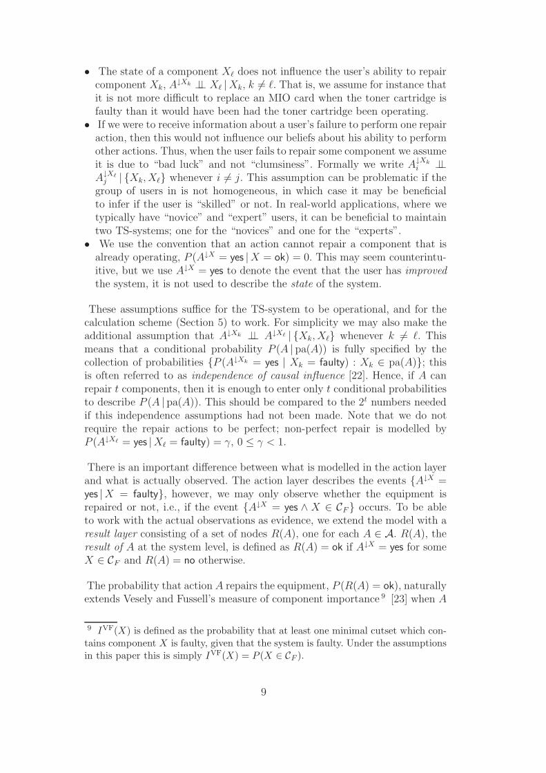
• The state of a component X` does not influence the user’s ability to repaircomponent Xk, A↓Xk ⊥⊥ X` |Xk, k 6= `. That is, we assume for instance thatit is not more difficult to replace an MIO card when the toner cartridge isfaulty than it would have been had the toner cartridge been operating.• If we were to receive information about a user’s failure to perform one repair
action, then this would not influence our beliefs about his ability to performother actions. Thus, when the user fails to repair some component we assumeit is due to “bad luck” and not “clumsiness”. Formally we write A↓Xk
i ⊥⊥A↓X`
j | Xk, X` whenever i 6= j. This assumption can be problematic if thegroup of users in is not homogeneous, in which case it may be beneficialto infer if the user is “skilled” or not. In real-world applications, where wetypically have “novice” and “expert” users, it can be beneficial to maintaintwo TS-systems; one for the “novices” and one for the “experts”.• We use the convention that an action cannot repair a component that is
already operating, P (A↓X = yes |X = ok) = 0. This may seem counterintu-itive, but we use A↓X = yes to denote the event that the user has improvedthe system, it is not used to describe the state of the system.
These assumptions suffice for the TS-system to be operational, and for thecalculation scheme (Section 5) to work. For simplicity we may also make theadditional assumption that A↓Xk ⊥⊥ A↓X` | Xk, X` whenever k 6= `. Thismeans that a conditional probability P (A | pa(A)) is fully specified by thecollection of probabilities P (A↓Xk = yes | Xk = faulty) : Xk ∈ pa(A); thisis often referred to as independence of causal influence [22]. Hence, if A canrepair t components, then it is enough to enter only t conditional probabilitiesto describe P (A | pa(A)). This should be compared to the 2t numbers neededif this independence assumptions had not been made. Note that we do notrequire the repair actions to be perfect; non-perfect repair is modelled byP (A↓X` = yes |X` = faulty) = γ, 0 ≤ γ < 1.
There is an important difference between what is modelled in the action layerand what is actually observed. The action layer describes the events A↓X =yes |X = faulty, however, we may only observe whether the equipment isrepaired or not, i.e., if the event A↓X = yes ∧ X ∈ CF occurs. To be ableto work with the actual observations as evidence, we extend the model with aresult layer consisting of a set of nodes R(A), one for each A ∈ A. R(A), theresult of A at the system level, is defined as R(A) = ok if A↓X = yes for someX ∈ CF and R(A) = no otherwise.
The probability that action A repairs the equipment, P (R(A) = ok), naturallyextends Vesely and Fussell’s measure of component importance 9 [23] when A
9 IVF(X) is defined as the probability that at least one minimal cutset which con-tains component X is faulty, given that the system is faulty. Under the assumptionsin this paper this is simply IVF(X) = P (X ∈ CF ).
9

can repair only one component X. Let IVF(X) be defined as the probabilityfor X to be critical, i.e., X ∈ CF , given that the equipment is faulty. Then
P (R(A) = ok)= P (X ∈ CF ) · P (A↓X = yes |X = faulty)
= IVF(X) · P (A↓X = yes |X = faulty). (1)
When A can repair a set of components, we have (with a slight abuse ofnotation):
P (R(A) = ok)= P
∨
X∈X
A↓X = yes
∧X ∈ CF
=∑C` ∈ C
IVF(C`)∐
X ∈ C` ∩ pa(A)
P (A↓X = yes |X = faulty),
where IVF(C`) is the probability that all components in C` are critical, i.e.,IVF(C`) equals the probability that C` is the actual cutset.
Regarding questions, we distinguish between symptom questions and config-uration questions. Symptom questions are used to examine possible failuremanifestations; an example from the printer-domain is “Does the printer
test-page print correctly?”. These questions are designed to shed light onthe fault at the cutset level, e.g., by trying to replicate the equipment’s faultymodus in other slightly different situations. (If the test-page prints correctlythe problem is probably related to the application generating the print job.)Symptom questions are connected to the MCS nodes in the domain, see thenode QS in Fig. 2. The edges are pointing in the direction of the causal influ-ence, i.e., from the MCS nodes to the questions. The parent set of a symptomquestion QS, pa(QS) ⊆ C, determines the set of MCSs that directly influencesthe likelihood of the different answers to the question.
Configuration questions are used to uncover the environment in which theequipment is embedded, by trying to reveal any configuration settings that areapplied. An example from our domain is “What operating system do you
use?”. Configuration settings does not directly relate to a given MCS, but maychange the likelihood for components to be operating. (If the operating systemis Linux, the printing problem is not related to the Windows printer drivers.)The edges connecting a configuration node to the system layer are thereforedirected from the configuration node to the components, see K in Fig. 2. Theuser may be unable to correctly answer questions regarding the configurationsettings. The answer to a configuration question is therefore modelled as arandom variable, see QK in Fig. 2. That is, we will receive information aboutQK (and not K directly) when the model is used, and QK is therefore neededexplicitly in the model together with K.
10

2.3 Building the TS-models
The theme of this paper is to find a close to optimal TS-strategy in a givenTS-model, but we will close this section by briefly touching upon the knowl-edge acquisition process used to generate the TS-model. 10 Building BNs hastraditionally been considered such a complex task that BN experts would haveto be deeply involved in the process. The BATS system consists of about 40separate Bayesian network models, each representing a specific failure-mode.Some models are quite small, but the largest contains about 80 actions and40 questions. To build these models we solely relied on a team of 6–7 experts.The number of models made it necessary to build a special tool for knowledgeacquisition, see [24]. This tool, which is termed BATS Author, is designed toensure that no knowledge about BNs is required to build the TS-models. Theinformation required to generate the models can be specified in a terminologyclose to the experts’ own, and the conditional probabilities can be expressedin the direction most natural for the expert. The BN structure is made s.t. theconditional independence statements encoded in the graph are easily verified.Skaanning [24] reports that all the models required to describe the failure-modes for another printer was built and validated in one man-month usingthis tool.
3 Action sequences
In this section we look at the situation where the only available troubleshoot-ing steps are actions. In this case the TS-strategy is simply a TS-sequence,i.e., a string of actions performed one after another until the equipment isrepaired. Let ε denote arbitrary evidence collected so far during troubleshoot-ing, i.e., a list of actions that all have failed to repair the equipment. Tobe more specific, we use ej to denote the evidence that the first j actionsin the sequence S = 〈A1, . . . , AN 〉 have all failed to repair the equipment,ej = R(Ai) = no : i = 1, . . . , j. If Ak solves the problem with certainty, thenP (ek) = 0, which reflects the fact that the TS-sequence is terminated afterthe k’th step. Note that e0 = ∅, and P (e0) = 1 as the equipment is assumedto be faulty at the beginning of the troubleshooting.
The expected cost of repair of a troubleshooting sequence S = 〈A1, . . . , An〉,where action Ai is allocated the cost Ci, is the mean cost until an actionsucceeds or all actions have been performed:
ECR(S) =N∑
i=1
Ci · P (ei−1) . (2)
10 This outline is based on Skaanning [24] and Jensen et al. [10]; further details canbe found in those papers.
11

A TS-sequence is said to be optimal if it achieves the minimum ECR ofall TS-sequences. Note that it might be slightly misleading to use the term“Expected cost of repair” as we consider a situation where a repair sequencemay fail to repair the equipment (since some actions may be imperfect, andtherefore fail to fix the critical components). Thus, a repair sequence S mayleave the equipment faulty, and the ECR is in this case the expected cost ofperforming the sequence and not of repairing the equipment (see the terminalnodes p, q and r in Fig. 1). The probability of a sequence failing to repairthe equipment is however determined by the set A only, and does not dependon the sequencing of the actions. Hence, as we are only interested in findingthe cheapest sequence, we will disregard this slight twist. 11 In this paper wefocus our attention towards the cost of performing the TS-strategy, and wewill continue to call this cost the ECR.
3.1 The greedy approach
Vesely and Fussell’s component importance is commonly regarded as the bestsearch heuristic when each component is repaired by a perfect action, and allrepair actions have the same cost. Furthermore, when the costs are unequal theVesely and Fussell’s component importance can be scaled by the action’s cost.The idea of using IFV(·) to sequence the actions generalizes to our situation,see Equation 1, and we therefore define an action’s efficiency in the followingway:
Definition 1. Let A ∈ A be a repair action, let CA be the cost of performingA, and let ε be the evidence compiled so far during troubleshooting. Theefficiency of A given ε is defined as
ef(A | ε) =P (R(A) = ok | ε)
CA.
The efficiency has an important property when verifying that a TS-sequenceS is sub-optimal:
Proposition 2. Let S = 〈A1, . . . , AN〉 be an optimal TS-sequence of actionsfor which the cost of each action is independent of the other actions taken.Then it must hold that ef(Ai | ei−1) ≥ ef(Ai+1 | ei−1).
11 If, on the other hand, we were interested in the monetary value of the expectedcost of the cheapest sequence, our approach would be misleading. To work in suchsituations, Breese and Heckerman [9] propose to introduce a new action namedCall Service as the final act in a TS-sequence. Performing this action will put theequipment back in operating modus, but presumably at a high cost since externalpersonnel is involved in fixing the problem.
12
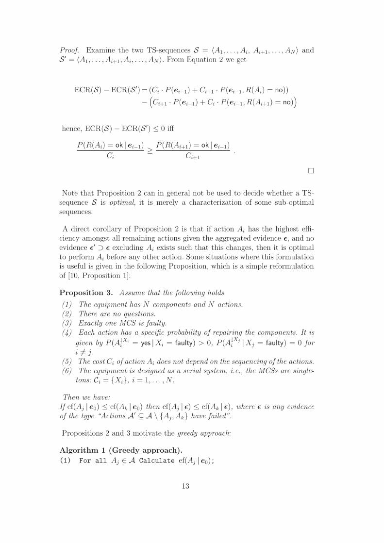
Proof. Examine the two TS-sequences S = 〈A1, . . . , Ai, Ai+1, . . . , AN〉 andS ′ = 〈A1, . . . , Ai+1, Ai, . . . , AN 〉. From Equation 2 we get
ECR(S)− ECR(S ′) = (Ci · P (ei−1) + Ci+1 · P (ei−1, R(Ai) = no))
−(Ci+1 · P (ei−1) + Ci · P (ei−1, R(Ai+1) = no)
)
hence, ECR(S)− ECR(S ′) ≤ 0 iff
P (R(Ai) = ok | ei−1)
Ci≥ P (R(Ai+1) = ok | ei−1)
Ci+1.
Note that Proposition 2 can in general not be used to decide whether a TS-sequence S is optimal, it is merely a characterization of some sub-optimalsequences.
A direct corollary of Proposition 2 is that if action Ai has the highest effi-ciency amongst all remaining actions given the aggregated evidence ε, and noevidence ε′ ⊃ ε excluding Ai exists such that this changes, then it is optimalto perform Ai before any other action. Some situations where this formulationis useful is given in the following Proposition, which is a simple reformulationof [10, Proposition 1]:
Proposition 3. Assume that the following holds
(1) The equipment has N components and N actions.(2) There are no questions.(3) Exactly one MCS is faulty.(4) Each action has a specific probability of repairing the components. It is
given by P (A↓Xii = yes |Xi = faulty) > 0, P (A
↓Xj
i |Xj = faulty) = 0 fori 6= j.
(5) The cost Ci of action Ai does not depend on the sequencing of the actions.(6) The equipment is designed as a serial system, i.e., the MCSs are single-
tons: Ci = Xi, i = 1, . . . , N .
Then we have:If ef(Aj | e0) ≤ ef(Ak | e0) then ef(Aj | ε) ≤ ef(Ak | ε), where ε is any evidenceof the type “Actions A′ ⊆ A \ Aj, Ak have failed”.
Propositions 2 and 3 motivate the greedy approach:
Algorithm 1 (Greedy approach).
(1) For all Aj ∈ A Calculate ef(Aj | e0);
13

(2) Let S be the list of actions ordered according to ef(· | e0);(3) Return S;
It follows that the greedy approach is optimal under the assumptions ofProposition 3. Note that it is not always optimal to sequence the actionsbased on the efficiencies. A counter-example is given below:
Example 4. Consider the domain described in Fig. 2 (with failure data fromFig. 3). We assume perfect repair actions, let Ci = 1 for all actions, and dis-regard the questions QS and QK . The greedy approach selects the sequence〈A3, A2, A4〉 with ECR = 1.58. The optimal sequence found by exhaustivesearch is 〈A2, A4〉, with ECR = 1.47. (Note that this result is not contra-dictory to Proposition 2; the efficiencies are calculated as ef(A2 | e0) = .529,ef(A3 | e0) = .624 and ef(A4 | e0) = .486, hence it is in accordance with Propo-sition 2 to start with A2 as long as it is not followed by A3.)
An obvious attempt to improve the results of Example 4 is to recalculate theefficiencies each time new evidence comes in. In this way we make sure thatall information available when the i’th step is to be chosen is actually takeninto account; recall that we use Bj to denote the j’th step in the strategy S:
Algorithm 2 (Greedy approach with recalculations).
(1) ε← ∅; A′ ← A1, . . . , AN; S = 〈·〉;(2) For i = 1 to N
(a) For all Aj ∈ A′ Calculate ef(Aj | ε);(b) Select Ak ∈ A′ s.t. ef(Ak | ε) is maximized;
(c) Bi ← Ak; A′ ← A′ \ Ak; ε← ε ∪ R(Ak) = no.(3) Return S;
Applied to the model in Example 4 this algorithm generates the sequence S =〈A3, A4, A2〉 with ECR = 1.53. This is better than the greedy approach, butstill not optimal. A result similar to Proposition 3 can be shown for arbitrarysized but disjoint MCSs if we assume that all actions are perfect:
Proposition 5. Let S = 〈A1, . . . , An〉 be a repair sequence for a trou-bleshooting problem fulfilling conditions 1 – 5 in Proposition 3. The MCSsare disjoint, Ci ∩ Cj = ∅, i 6= j, and all repair actions are perfect, i.e.,
P (A↓Xii = ok |Xi = faulty) = 1 for i = 1, . . . , N . Let S be the output of
Algorithm 2. Then S is an optimal repair sequence.
It should be emphasized that the actions are assumed to be perfect in Propo-sition 5. When the actions are non-perfect, optimality is no longer assured, ascan be seen from the example below:
Example 6. Consider a TS-model with two cutsets C1 = X1, X2 andC2 = X3, X4, X5. Let P (Xi = faulty) = 3 · 10−6 for i = 1, 3, 4, 5 and P (X2 =
14

faulty) = 7 · 10−6. Each component Xi is repaired by a dedicated action Ai.Let the cost of the actions be C1 = 9, C2 = 12, and Ci = 10 for i = 3, 4, 5.Finally, P (X↓A1
1 = ok |X1 = faulty) = .9, P (X↓Aii = ok |Xi = faulty) = .98 for
i = 2, 3, and P (X↓Aii = ok |Xi = faulty) = .95 for i = 4, 5. Then Algorithm 2
returns S1 = 〈A5, A1, A3, A4, A2〉 with ECR(S1) = 14.95, whereas the optimalsequence is S2 = 〈A5, A3, A4, A1, A2〉 with ECR(S2) = 14.84.
3.2 Dependent actions
The crucial step when optimality is proven in the setting of Propositions 3is the fact that no evidence obtained during troubleshooting can change theordering of the remaining actions under consideration; the residual probabilitymass, i.e., the probability P (R(Ai) = ok | ei−1), is absorbed uniformly by allthese actions. Hence, the initial ordering of two actions, Ai ≺ Aj , say, cannotchange when some new evidence R(Ak) = no, Ak 6∈ Ai, Aj arrives. In thegeneral case, however, the ordering of a subset of actions A′ ⊂ A may dependon what evidence ε is collected, even if ε does not contain explicit informationabout any of the actions in A′. We call this situation dependent actions [25].
A domain for which the cost of an action does not depend on the sequence ofactions taken is said to have dependent actions whenever there exists actionsAi, Aj and Ak s.t.
ef(Ai | ∅)ef(Aj | ∅) 6=
ef(Ai |R(Ak) = no)
ef(Aj |R(Ak) = no).
A domain has dependent actions if there exists two actions Ai and Aj s.t.pa(Ai) ∩ pa(Aj) 6= ∅ or there exists two actions Ai and Aj, two componentsXk ∈ pa(Ai) and X` ∈ pa(Aj), and an MCS Cm s.t. Xk, X` ⊆ Cm. An exam-ple from the printer domain is the action-pair “Reseat toner cartridge.”and “Change toner cartridge.” as both may solve problems related to badseating of the cartridge.
Examples 4 and 6 showed that Vesely and Fussell’s component importance isnot optimal in general when the domain has dependent actions. This is hardlya surprise, since the problem of finding an optimal troubleshooting strategy isknown to be NP-hard in this case [11]. To try to improve a suboptimal strat-egy we employ an adapted version of a standard algorithm for combinatorialoptimization (similar to the algorithm presented by Norstrøm et al. [7]). Thisalgorithm starts from an initial seed, and iteratively improves this sequenceuntil it converges to a local optimum. Note that B
(i)k (Step 2a) denotes the k’th
TS-step in the action sequence S when starting the i’th step of the iteration.Note also that the algorithm is said to converge (Step 3) when the ECR of thefound sequence is not lower than the ECR of the sequence found previously.
15

Algorithm 3 (Discrete optimization).
(1) Initialization: S ← 〈B1, . . . , BN〉 for some ordering of A;(2) For i = 1 to N
(a) For j = i to NRj ← 〈B(i)
1 , . . . , B(i)i−1, B
(i)j , B
(i)i , . . . , B
(i)j−1, B
(i)j+1, . . . , B
(i)N 〉;
(b) Select j0 ∈ [i . . . N ] s.t. ECR(Rj0) is minimized;
(c) S ← Rj0;
(3) If not converged then goto 2;
(4) Return S;
A sequence S = 〈A1, A2, . . . , Ai, . . . , Aj, . . . , AN〉 is a local optimum if, when-ever we insert Aj before Ai (j > i) in S to obtain S ′ = 〈A1, A2, . . . , Ai−1, Aj ,Ai, . . . , Aj−1, Aj+1, . . . , AN 〉, then ECR(S) ≤ ECR(S ′). It is obvious thatAlgorithm 3 converges to a local optimum since ECR(S) is guaranteed to benon-increasing after each loop of the algorithm (the algorithm can decide tostay put by selecting j0 s.t. Rj0 = S in Step 2b). It is however not guaranteedthat the algorithm converges to the globally optimal sequence. The crucialchoice to be made in Algorithm 3 is the initialization of S in Step 1. To ensurequick convergence to an approximately optimal solution, it can be beneficialto select a seed sequence that is close to the optimum. A natural choice isto initialize S as found by Algorithm 2. It is however easy to see that thissequence is a local optimum itself (confer Proposition 2), and it will thereforenot be improved by Algorithm 3. Instead, we suggest to initialize the actionsequence by ordering wrt. the observation-based efficiency (obef). We outlinethe derivation of the observation-based efficiency [25] below.
Consider a situation where the evidence ε has been collected and it has beendecided that the next action to perform is A. To calculate the observation-based efficiency, the TS-system should consider what information can be gainedabout the failed equipment by just getting to know that A does not solve theproblem, and more importantly, the value of this information. It is natural toquantify this value as the difference in ECR between two degenerate models:i) The TS-system where the collected evidence is ε′ = ε, R(A = no) and ii)The TS-system where A has been made unavailable, but where the collectedevidence is ε′′ = ε. Assume that the sequence of remaining actions when givenevidence ε′ is S(ε′) and that the sequence of the actions when given evidence ε′′
and A is unavailable is S(ε′′). We define the conditional ECR of the sequenceS = 〈A1, . . . , AN〉 given ε′ as ECR(S | ε′) =
∑Nj=1 Cj · P (ej−1 | ε′). Finally, we
define the value of the information contained in the event that R(A) = nogiven the current evidence ε as
VOI(R(A) = no | ε) = ECR(S(ε′) | ε′)− ECR(S(ε′′) | ε′),
i.e., VOI(R(A) = no | ε) is the difference of the expected cost of the strategiesS(ε′) and S(ε′′). Note that both expected costs are calculated conditioned on
16

ε′, the evidence actually collected as the two strategies are considered to beemployed.
To recapitulate, we want to consider the value of information an action thatfails has to offer when we determine how to sequence the actions. This amountis calculated as VOI(R(A) = no | ε), and we receive this gain with probabil-ity P (R(A) = no | ε). If we regard this amount as a refund, it is natural toapproximate the “real” cost of action A as
CA = CA − P (R(A) = no | ε) · VOI(R(A) = no | ε).
CA is the cost we “spend” by performing A; CA−CA is the expected reductionin ECR of the remaining sequence of action, which is obtained by learning thatA fails. It is argued by Langseth and Jensen [25] that if one couples Definition1 with Algorithm 2, one implicitly assumes that VOI(R(A) = no | ε) = 0. Onthe other hand, if CA is used as the cost of A in the efficiency calculation, thiswill change the troubleshooting strategy in a way that attempts to incorporatethe actual value of the information we receive. This leads to the definition ofthe observation-based efficiency:
Definition 7. Let A ∈ A be a repair action, let the cost of A be CA, and let εbe the evidence compiled so far during troubleshooting (i.e., not containing A).Let VOI(R(A) = no | ε) be the value of information A will have if it fails (byaltering the sequencing of the remaining actions). Then the observation-basedefficiency of A given ε is:
obef(A | ε) =P (R(A) = ok | ε)
CA − P (R(A) = no | ε) · VOI(R(A) = no | ε) .
An algorithm that orders the actions according to the observation-based effi-ciency does in general not offer an optimal solution; a sequence ordered in thisway may even violate the optimality check of Proposition 2. This is howeverof minor importance, as we only use the sequence as a seed to Algorithm 3and do not regard it as a final solution on its own. Note however, that theprobability update is proportional under the assumptions in Proposition 3,which means that VOI(R(A) = no | ε) = 0 in this case. The observation-basedefficiency is therefore exact under the assumptions of Proposition 3. “Cyclepower.” is an example of an action from our domain which has high value ofinformation. Power cycling repairs many temporal problems, and ruling theseout can be very beneficial for the future troubleshooting.
A problem with Definition 7 is that VOI(R(A) = no | ε) cannot be calculatedunless one is able to correctly sequence all remaining actions (after perform-ing A) in order to calculate ECR(S(ε′) | ε′) and ECR(S(ε′′) | ε′); a computa-tionally prohibitive task. Langseth and Jensen discuss two approximations of
17

VOI(R(A) = no | ε): One based on the Shannon entropy of the efficiencies ofthe remaining actions, and the computationally simpler approach to use themyopic ordering of actions (i.e., based on Definition 1), see [25] for details.
Table 1 shows results of a small simulation study. Three troubleshootingmodels have been used: The example model of Fig. 3 (with N = 5 actions andR = 4 cutsets), the CPQRA model [26] (N = 25, R = 20) and Norstrøm etal.’s example [7] (N = 6, R = 4). For each model the actions’ costs and thefailure probabilities of the components have been randomized. Additionally,the probability of an action to successfully repair a component in its parentset was randomly selected in the interval [0.9, 1.0]. Then Algorithm 2 andAlgorithm 3 were run, and compared by difference in ECR. 12 The simulationswere run for 500 iterations. The reported numbers give the relative number oftimes Algorithm 2 found a result inferior to that of Algorithm 3 (Rel.num.),the average relative difference in ECR in those runs (Avg.rel.diff.), and themaximum relative difference in ECR (Max.rel.diff.).
Rel.num. Avg.rel.diff. Max.rel.diff.
Example model of Fig. 3 8.2% 4.0% 7.5%
The CPQRA model [26] 9.4% 4.2% 8.2%
Norstrøm et al.’s example [7] 4.0% 4.9% 9.2%
Table 1Algorithm 2 and Algorithm 3 are compared through a small simulation study.
The results in Table 1 show that even for the relatively small models wehave considered, a strategy generated by the Vesely and Fussell’s componentimportance (Algorithm 2) fails fairly frequently, and the additional cost offollowing an inferior sequence may be considerable.
As it is NP-hard to find the optimal repair sequence, Algorithm 3 is notinfallible; it may sometimes be stuck in sub-optimal solutions. This did forinstance happen for the CPQRA model (see Table 1), where Algorithm 3 evenwas inferior to Algorithm 2 in 1.2% of the simulations, with maximum relativecost difference equal to 2.1%.
4 Questions
When we add questions to our TS-model, the strategy is represented by astrategy tree, see Fig. 1. Note that the ECR cannot be calculated by Equation
12 Algorithm 3 was initialized by the sequence obtained when the actions wereordered according to the observation-based efficiency; the value of information wasapproximated by employing a myopic strategy.
18
2 in this case, instead we use a recursive calculation scheme to compute theexpected cost of repair:
Proposition 8. Let S be a TS-strategy which starts with the step B(1) andthen continues with the strategy conditioned on the possible outcomes of B(1).Then the ECR of S can be calculated recursively as:
ECR(S) = C(1) +∑
b(1)∈sp(B(1))
P(B(1) = b(1)
)· ECR
(S |B(1) = b(1)
). (3)
where C(1) is the cost of step B(1) and ECR(S |B(1) = b(1)
)is the ECR of
the sub-tree S following the branch for which B(1) = b(1). The recursion isterminated by ECR (∅ | ·) = ECR (· |R(Aj) = ok) = 0.
The obvious way to decide whether it pays to pose a question Q, is to calcu-late the value of information for that particular question. Let the strategy bedefined as 〈Q,S〉, where S is the optimal strategy conditioned on the answerto the question Q, and let S ′ be the optimal strategy when we are refused topose Q. We define VOI(Q) as:
VOI(Q) = ECR(S ′)−∑q∈sp(Q)
P (Q = q) · ECR(S |Q = q) .
The system should pose the question if VOI(Q) > CQ.
A problem with this approach is that we must correctly position all other ques-tions in the strategy before we can calculate ECR(S ′) and ECR(S |Q = q);this will lead to a too expensive recursion. Breese and Heckerman [9] pro-pose to use a myopic approach to this problem: Assume that it is sufficientto sequence only actions when VOI(Q) is to be calculated, i.e., one shouldconsider the effect of the question Q only on the sequencing of actions, anddisregard the effect of the other questions. The two action sequences S and S ′
are then approximated by ordering the actions according to their efficienciesby Algorithm 2. In [10] it is argued that this approach will over-rate the effectof the question, because one in this case only compares the effect of askingthe question now, with ECRNow = CQ +
∑q∈sp(Q) P (Q = q) · ECR(S |Q = q),
or never, ECRNever = ECR(S ′). The decision rule is to pose the question iff
ECRNow < ECRNever. (4)
Jensen et al. [10] argue that one should also compare ECRNow to the ECRof a strategy starting with what appears to be the best action, followed by Q,and thereafter a TS-sequence S ′′, which depends on the outcome of Q. Thisapproach has ECR given by
19

ECRA,Q(A, Q,S ′′) = CA + P (R(A) = no) · CQ +∑q∈sp(Q)
P (Q = q, R(A) = no) · ECR(S ′′ |Q = q, R(A) = no) .
The question should be posed iff
ECRNow < minECRA,Q(A, Q,S ′′), ECRNever. (5)
N M Optimal Alg. 2 + Eq. 5 Alg. 2 + Eq. 4 Alg. 2
6 2 433.24 442.39 442.43 444.54
9 3 129.21 129.21 205.54 155.10
11 3 106.20 108.07 111.75 116.80
12 3 38.38 40.01 52.86 43.05
13 4 124.32 125.56 125.94 300.85
14 4 115.41 115.86 116.74 236.58
9 9 70.67 77.67 76.53 121.10
16 5 161.38 162.25 162.49 286.75
10 10 250.45 256.96 445.93 479.96
Avg. rel. diff. from opt. 2.51% 21.5% 59.16%
Table 2Empirical comparison of the effect of including questions into 9 of the BATS TS-
models. The results are extended from those reported by Vomlel [27].
To emphasize the importance of including questions in the troubleshootersystem we reproduce and extend a set of experimental results from Vomlel [27].We have examined 9 of the troubleshooter models included in the BATS tool;for each of them we calculated the ECR of the optimal TS-strategy, the ECR ofthe TS-strategy produced when combining Algorithm 2 with Equation 5, theECR of the TS-strategy produced when combining Algorithm 2 with Equation4, and finally the ECR of the TS-sequence generated from Algorithm 2 whenquestions were disregarded. The models we used for testing were moderatelysized with N (number of actions) ranging from 6 to 16 and M (number ofquestions) in the interval from 2 to 10. The results clearly show how importantthe questions are in these real-life TS-models, and they also indicate thatthe approximations made in Algorithm 2 combined with the decision rule ofEquation 5 may be quite reasonable.
20
5 Calculation scheme
In this section we will consider how to perform the required calculation in themodel. As the TS-system will continuously interact with the user, it is impor-tant that the system can perform its calculations in “real time” (that is, thecalculations should be performed using an amount of time that seems negligi-ble to the user). The important point to make is that performing calculationsis in principle of time complexity exponential in the number of componentsin the model. It is therefore crucial to identify the “idle time” of the system(i.e., the time when the user is not interacting with it), and use those pointsin time to perform the calculations. Idle time is available before the systemis put into use, and at times when the user is busy performing an action ortrying to find information to answer a question. Before the system is ready tobe used it has to go through an initialization phase, which basically amountsto calculating the initial probabilities for each component to be in its faultystate given that the equipment is faulty, the probabilities for the actions tobe successful, and the initial beliefs regarding possible answers to the differ-ent questions. These calculations can be performed off-line and are thus notsubject to speed requirements. In the following we will therefore focus on howto incorporate information from the performed TS-steps into the system, thatis, how to update the probability distributions when the compiled evidence εis extended.
5.1 Action sequences
First we will look at TS-systems that only consists of actions, and describe amethod for calculating P (R(A) = ok | ε) for an action A ∈ A where ε is someevidence not involving A. Next, we will describe a method to calculate P (ε)(required by the ECR-calculations, see Equation 2). Note that the evidenceε will contain only a list of failed actions, i.e., ε = R(A) = no : A ∈ A′.If an action is successful, the troubleshooting ends, and there is no need toincorporate that evidence into the system.
The key point during the calculations is that of conditional independence.Let nd(V ) be the non-descendants of V in a directed graph G; Y ∈ nd(X) iffthere is no directed path X → . . . → Y in G. An important result we shalluse frequently is that V ⊥⊥ nd(V ) | pa(V ) for any variable V ∈ V.
The backbone of our calculating scheme is the observation that if we know thatCi is the actual cutset, then it is easy to calculate the success probabilities giventhe evidence ε. It turns out that P (R(A) = ok | Ci = faulty, ε) = P (R(A) =ok | Ci = faulty), see Lemma 9 below. Since the actual cutset is not knownduring troubleshooting, we use
21

P (R(A) = ok | ε)=∑C`∈C
P (R(A) = ok | C` = faulty, ε) · P (C` = faulty | ε)
=∑C`∈C
P (R(A) = ok | C` = faulty) · P (C` = faulty | ε)
to calculate P (R(A) = ok | ε). Next, we formalize the above statement:
Lemma 9. Let A ∈ A be a repair action, and let evidence compiled duringtroubleshooting be denoted by ε, ε = R(Ai) = no : Ai ∈ A′ (A 6∈ A′). As-sume that the user’s ability to repair one component X does not depend on thestate of the other components, A↓X ⊥⊥ X ′ |X for all X ′ ∈ X \X, and that in-formation about the user failing to perform one repair action will not influenceour beliefs about his ability to perform other actions, A↓Xk
i ⊥⊥ A↓X`j | Xk, X`
whenever i 6= j. Then P (R(A) | Cm = faulty, ε) = P (R(A) | Cm = faulty). Thatis, the evidence ε does not influence R(A) when conditioning on the actualMCS.
Proof. First, notice that if P (R(A) = ok | Cm = faulty) = 0, then no evidenceε can change this belief. Hence, P (R(A) | Cm = faulty, ε) = P (R(A) | Cm =faulty) if A cannot repair any component in Cm. Next, assume that the actionA can repair components in only one MCS, C`. If C` = faulty, then all com-ponents Xj ∈ C` are in their faulty state. Hence, we have evidence on the setpa(A), and since ε only contains non-descendant of A by construction of thedomain model, A ⊥⊥ ε | C` = faulty. It follows that R(A)⊥⊥ε | C` = faulty,and therefore P (R(A) | C` = faulty, ε) = P (R(A) | C` = faulty). (See A1 inFig. 5; the probability for A1 to repair the equipment is determined by thestate of C1 only. If C1 is the actual MCS then A1 repairs the equipment withprobability P (A↓X1
1 = yes |X1 = faulty) no matter what actions have earlierbeen performed; if C1 is not faulty, then A1 can never repair the equipment.)
In the general case action A can repair more than one MCS. To see that theLemma holds also in this case, we introduce the random variable ζ(C`), which isdefined s.t. ζ(C`) = yes if Xi = faulty : Xi ∈ C` ∧Xj = ok : Xj 6∈ C`; ζ(C`) =no otherwise. Notice that the effect of conditioning on the event ζ(C`) = yes isthat all X ∈ X are given evidence, and by construction of the domain model,the set pa(A) ⊆ X is instantiated. Hence P (R(A) = ok | ζ(C`) = yes, ε) =P (R(A) = ok | ζ(C`) = yes). Since A↓X ⊥⊥ X ′ |X for X ′ ∈ X \ X, wehave P (R(A) | C` = faulty, ε) = P (R(A) | ζ(C`) = yes, ε). Finally, it followsthat P (R(A) | C` = faulty, ε) = P (R(A) | C` = faulty). (Look at action A3 inFig. 5, and assume that C3 is known to be faulty, which means that X3 =X4 = faulty. The event R(A3) = ok is in this case equivalent to A↓X3
3 =yes∨A↓X4
3 = yes. So far we only have observations on X3 and X4; X1 and X2
are not instantiated. Hence, information may flow from R(A1) to R(A3), and
22

thereby break the required independence (which is problematic if R(A1) =
no has been observed). The assumption A↓Xj
i ⊥⊥ Xk |Xj does however justifythat we may set X1 = X2 = ok without changing the required probabilityP (R(A3) | C3 = faulty, ε). All flow of information from any compiled evidenceε to R(A3) is blocked when these stochastic variables are instantiated, andthe desired conditional independence follows.)
X2
C2 C3
L
C1
X1 X3
A3A1
R(A1) R(A2) R(A3)
X4
A2
Fig. 5. Example TS-model to exemplify the proof of Lemma 9.
We utilize Lemma 9 to calculate the probability that an action A ∈ A repairsthe equipment:
P (R(A) | ε) =∑C` ∈ C
P (R(A) | C` = faulty) · P (C` = faulty | ε) . (6)
That is, calculating P (R(A) | ε) amounts to finding P (R(A) | C` = faulty) andP (C` = faulty | ε) for all C` ∈ C. The values of P (R(A) | C` = faulty) can easilybe calculated from the model description before the troubleshooting starts,whereas P (C` = faulty | ε) must be calculated in each case.
We now show that Lemma 9 can be used also to calculate P (C` = faulty | ei)rather efficiently; recall that ei is used to denote the evidence that the first iactions in the sequence S = 〈A1, . . . , AN〉 have all failed to repair the equip-ment. We first use Bayes’ rule to investigate how to update this probabilitywhen new evidence R(Ai) = no is received and appended to the compiledknowledge ei−1:
P (C` = faulty | ei)= P (C` = faulty | ei−1, R(Ai) = no)
=P (R(Ai) = no | C` = faulty, ei−1) · P (C` = faulty | ei−1)
P (R(Ai) = no | ei−1)
=P (R(Ai) = no | C` = faulty) · P (C` = faulty | ei−1)
P (R(Ai) = no | ei−1). (7)
23

P (R(Ai) = no | ei−1) is just a normalization constant in this calculation, whichcan be found by
P (R(Ai) = no | ei−1) =∑Ck ∈ C
P (R(Ai) = no | Ck = faulty)·P (Ck = faulty | ei−1) .
Hence P (C` = faulty | ei) can be calculated by expanding the evidence itera-tively. The first step of this procedure requires the a priori distribution overthe MCSs, P (C` = faulty | e0). This distribution should be calculated by a fullpropagation in the Bayesian network, see [21]; remember that this propagationcan be performed off-line (i.e., before troubleshooting starts). The evidence ei
is then incorporated by using Equation 7 until we obtain P (C` = faulty | ei).This means that calculating P (R(A) | ei) is of complexity O(R), where R isthe number of MCSs in the domain if we have stored P (C` = faulty | ei−1). Asa consequence, the complexity of Algorithm 1 is O(NR + N log(N)) and thecomplexity of Algorithm 2 is O(N(NR + N)) = O(N2R).
Next, we look at how to calculate P (ei); a number required by the ECRcalculations, see Equation 2. This can be done by using the identity P (ei) =P (R(Ai) = no | ei−1)P (ei−1) and make the calculations iteratively; P (R(Ai) =no | ei−1) is given by Equation 6; P (e0) = 1 by convention. Calculating P (ei)is therefore of complexity O(R) if we store the values P (ei−1). In total, thecalculation of ECR is thus of time complexity O(NR).
The time complexity of generating a full action sequence based on the obser-vation-based efficiency (Definition 7) is dominated by the expensive calcula-tions required to find VOI(· | ε). If this value is approximated by calculatingthe ECR of the sequence generated by Algorithm 2, then the time complexityof generating a complete action sequence by the observation-based efficiency isO(N3R). If one settles for the cruder approximation offered by Algorithm 1 thetime complexity of generating the sequence is reduced to O (N2(log(N) + R)).
The time complexity of Algorithm 3 is given by the complexity of the initial-ization and the cost of O(N2) calculations of ECR. This means that the totalcomplexity of Algorithm 3 when initialized according to the obef-sequenceis O(N3R). This should be compared to the corresponding calculations per-formed in a fault tree, which Norstrøm et al. [7] report to be O(N23N).
5.2 Questions
In this section we consider the cost of belief updating when the TS-model isextended to incorporate questions.
24
5.2.1 Symptom questionsWe start the treatment of questions by considering symptom questions. Recallthat symptom questions are used to examine possible failure symptoms; theyare connected to the system layer at the MCS level, with edges directed fromproblem causes to the questions, see QS in Fig 2. By construction, the parentset of a symptom question QS in our BN representation is therefore restrictedto the MCS nodes, pa(QS) ⊆ C. Furthermore, symptom questions do not havedescendants in the graph. It follows that QS ⊥⊥ V \ C, QS |C. Therefore,to calculate the effect of a symptom question on the remaining strategy, itis only required to calculate the effect on the distribution over the MCSs,P (C` = faulty |QS = q, ε). This can be done by using Bayes’ rule:
P (C` = faulty |QS = q, ε)=P (QS = q | C` = faulty, ε) · P (C` = faulty | ε)
P (QS = q | ε)=
P (QS = q | C` = faulty) · P (C` = faulty | ε)P (QS = q | ε) , (8)
where P (QS = q | ε) =∑Ck ∈ C P (QS = q | Ck = faulty) · P (Ck = faulty | ε).
Hence, the complexity of calculating P (C` = faulty |QS = q, ε) from P (C` =faulty | ε) isO(R). If we assume that the ordering of actions needed to calculatethe ECR values in the decision rule of Equation 5 is based on Algorithm 2,then a question can be evaluated in time complexity O(N2R). Note that thecalculations will require the computation of ECR for several action sequences(described in Section 5.1); one for each possible answer to the question.
Note that QS ⊥⊥ V \ C, QS |C implies that symptom questions will notcorrupt the calculations of R(A | ε) in Equation 6; we can use that calculationscheme to calculate R(A | ε) even when the evidence ε contains answers tosymptom questions.
5.2.2 Configuration questionsConfiguration questions are designed to highlight the likelihood of compo-
nent failures by uncovering the environment in which the failed equipmentis embedded. Configuration nodes are connected to the system layer via thecomponent layer, with edges directed from question to components, see K inFig. 2. The answer to the question is modelled as a random variable dependenton the configuration, see QK in Fig. 2.
As for symptom questions, we are interested in evaluating QK accordingto Equation 5. First, however, we note that R(A) ⊥⊥ ε | C` = faulty alsowhen configuration questions have been posed, QK = q ⊆ ε. Recall thatP (R(A) | ε′, C` = faulty) = P (R(A) | C` = faulty) when ε′ is a list of ac-tions (not containing A) that have failed. This result trivially extends to the
25
case where ε contain answers to questions because configuration questions arenon-descendants of the actions’ result nodes. We can therefore calculate theefficiency of an action using Equation 6 also in the case when configurationquestions have been answered. Similarly, we can calculate the ECR-valuesrequired to evaluate a configuration question QK (according to Equation 5)efficiently by incorporating the effect of a question QK at the cutset nodes byusing Equation 8.
Special attention is however required for the case when one configurationquestion QK1 is evaluated, and the evidence ε already contains the answer toanother configuration question QK2 together with a list of failed actions ε′,ε = QK2 = q, ε′. The answer to the two configuration questions QK1 andQK2 are not independent given the actual cutset; we have P (QK1 = q | ε, C` =faulty) = P (QK1 = q |QK2 = q, C` = faulty). Hence, we must take the answersto all earlier configuration questions into account when we want to calculateP (QK1 = q | ε). A consequence of this conditional dependence is that the fastrules to incorporate new evidence into the system, see Equations 7 and 8,cannot be generalized to evidence containing configuration questions if thedistribution of other configuration questions should be updated correctly. Wetherefore have to perform a propagation in the model as soon as a configurationquestion is answered; note that it is not required to perform any propagationsas long as the TS-system just considers to pose the question. The complexity ofevaluating a configuration question is therefore O(N2R); the time complexityof incorporating the answer into the system is exponential in the number ofcomponents.
6 Concluding remarks
We have described a decision-theoretic troubleshooting system, which buildson a Bayesian network describing the faulty equipment and its surroundings.The expressive power of the BN framework outperforms that of more com-monly used model description paradigms as, e.g., fault trees, see [20]. Weutilized this to make a rich description of the troubleshooting domain, whichmay include, e.g., non-perfect actions and information-gathering troubleshoot-ing steps. Finally, we showed how our BN models allow fast calculation of theprobabilities required to generate a reasonable troubleshooting strategy.
Acknowledgements
We would like to thank our project coworkers, in particular Claus Skaanning,Jirı Vomlel, and Olav Bangsø, for interesting discussions. Jirı Vomlel alsosupplied the software used to generate the results in Table 2. An anonymousreferee gave comments that helped improving the paper.
26

References
[1] W. E. Vesely, Fault tree handbook, Tech. Rep. NUREG-0492, US NuclearRegulatory Committee, Washington DC (1981).
[2] Q. Zhang, Q. Mei, A sequence of diagnosis and repair for a 2-state repairablesystem, IEEE Transactions on Reliability R-36 (1) (1987) 32–33.
[3] J. Kalagnanam, M. Henrion, A comparison of decision analysis and expertrules for sequential analysis, in: Uncertainty in Artificial Intelligence 4, North-Holland, New York, 1990, pp. 271–281.
[4] W. Xiaozhong, Fault tree diagnosis based on Shannon entropy, ReliabilityEngineering and System Safety 34 (1991) 143–167.
[5] W. Xiaozhong, R. M. Cooke, Optimal inspection sequence in fault diagnosis,Reliability Engineering and System Safety 37 (1992) 207–210.
[6] R. Reinertsen, W. Xiaozhong, General inspection strategy for fault diagnosis–minimizing the inspection costs, Reliability Engineering and System Safety48 (3) (1995) 191–197.
[7] J. Norstrøm, R. M. Cooke, T. J. Bedford, Value of information basedinspection-strategy of a fault-tree, in: Proceedings of the tenth EuropeanConference on Safety and Reliability, A. A. Balkema, Munich, Germany, 1999,pp. 621–626.
[8] S. Srinivas, A polynomial algorithm for computing the optimal repair strategyin a system with independent component failures, in: Proceedings of theEleventh Annual Conference on Uncertainty in Artificial Intelligence, SanFrancisco, CA., 1995, pp. 515–522.
[9] J. S. Breese, D. Heckerman, Decision-theoretic troubleshooting: A frameworkfor repair and experiment, in: Proceedings of the Twelfth Conference onUncertainty in Artificial Intelligence, Morgan Kaufmann Publishers, SanFrancisco, CA., 1996, pp. 124–132.
[10] F. V. Jensen, U. Kjærulff, B. Kristiansen, H. Langseth, C. Skaanning, J. Vomlel,M. Vomlelova, The SACSO methodology for troubleshooting complex systems,Artificial Intelligence for Engineering, Design, Analysis and Manufacturing15 (5) (2001) 321–333.
[11] M. Sochorova, J. Vomlel, Troubleshooting: NP-hardness and solution methods,in: The Proceedings of the Fifth Workshop on Uncertainty Processing,WUPES’2000, Jindrichuv Hradec, Czech Republic, 2000, pp. 198–212.
[12] C. Skaanning, F. V. Jensen, U. Kjærulff, P. Pelletier, L. Ropstrup-Jensen,Printing system diagnosis: A Bayesian network application, Workshop onPrinciples of Diagnosis, Cape God, MA. (2000).
[13] J. Pearl, Probabilistic Reasoning in Intelligent Systems: Networks of PlausibleInference, Morgan Kaufmann Publishers, San Mateo, CA., 1988.
27
[14] F. V. Jensen, Bayesian Networks and Decision Graphs, Springer Verlag, NewYork, 2001.
[15] R. E. Barlow, Using influence diagrams, in: C. A. Clarotti, D. V. Lindley (Eds.),Accelerated life testing and experts’ opinions in reliability, 1988, pp. 145–157.
[16] H. J. Call, W. A. Miller, A comparison of approaches and implementationsfor automating decision analysis, Reliability Engineering and System Safety 30(1990) 115–162.
[17] J. G. Torres-Toledano, L. E. Sucar, Bayesian networks for reliability analysis ofcomplex systems, Lecture Notes in Artificial Intelligence 1484 (1998) 195–206.
[18] N. Fenton, B. Littlewood, M. Neil, L. Strigini, A. Sutcliffe, D. Wright, Assessingdependability of safety critical systems using diverse evidence, IEE ProceedingsSoftware Engineering 145 (1) (1998) 35–39.
[19] P. H. Ibarguengoytia, L. E. Sucar, E. Morales, A probabilistic model approachfor fault diagnosis, in: Eleventh International Workshop on Principles ofDiagnosis, Morelia, Mexico, 2000, pp. 79–86.
[20] A. Bobbio, L. Portinale, M. Minichino, E. Ciancamerla, Improving theanalysis of dependable systems by mapping fault trees into Bayesian networks,Reliability Engineering and System Safety 71 (3) (2001) 249–260.
[21] F. V. Jensen, S. L. Lauritzen, K. G. Olesen, Bayesian updating incausal probabilistic networks by local computations, Computational StatisticsQuarterly 4 (1990) 269–282.
[22] D. Heckerman, J. S. Breese, A new look at causal independence, in: Proceedingsof the Tenth Annual Conference on Uncertainty in Artificial Intelligence,Morgan Kaufmann Publishers, San Francisco, CA., 1994, pp. 286–292.
[23] W. E. Vesely, A time-dependent methodology for fault tree evaluation, NuclearEngineering and design 13 (1970) 339–360.
[24] C. Skaanning, A knowledge acquisition tool for Bayesian-network trouble-shooters, in: Uncertainty in Artificial Intelligence: Proceedings of the SixteenthConference, Morgan Kaufmann Publishers, San Francisco, CA., 2000, pp. 549–557.
[25] H. Langseth, F. V. Jensen, Heuristics for two extensions of basictroubleshooting, in: Seventh Scandinavian Conference on Artificial Intelligence,SCAI’01, Frontiers in Artificial Intelligence and Applications, IOS Press,Odense, Denmark, 2001, pp. 80–89.
[26] Center for Chemical Process Safety, Guidelines for Chemical ProcessQuantitative Risk Analysis, American Institute of Chemical Engineers, NewYork, 1989.
[27] J. Vomlel, On quality of BATS troubleshooter and other approximativemethods, Technical report, Department of Computer Science, AalborgUniversity, Denmark (2000).
28

III
Classification using Hierarchical Naıve Bayes models

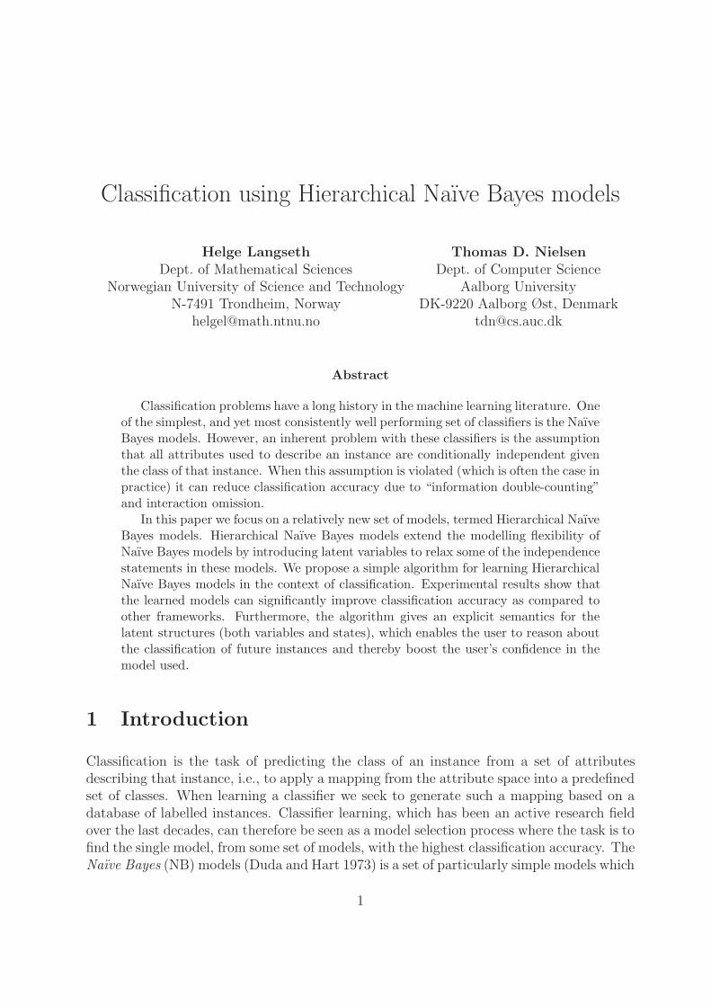
Classification using Hierarchical Naıve Bayes models
Helge Langseth Thomas D. NielsenDept. of Mathematical Sciences Dept. of Computer Science
Norwegian University of Science and Technology Aalborg UniversityN-7491 Trondheim, Norway DK-9220 Aalborg Øst, Denmark
[email protected] [email protected]
Abstract
Classification problems have a long history in the machine learning literature. Oneof the simplest, and yet most consistently well performing set of classifiers is the NaıveBayes models. However, an inherent problem with these classifiers is the assumptionthat all attributes used to describe an instance are conditionally independent giventhe class of that instance. When this assumption is violated (which is often the case inpractice) it can reduce classification accuracy due to “information double-counting”and interaction omission.
In this paper we focus on a relatively new set of models, termed Hierarchical NaıveBayes models. Hierarchical Naıve Bayes models extend the modelling flexibility ofNaıve Bayes models by introducing latent variables to relax some of the independencestatements in these models. We propose a simple algorithm for learning HierarchicalNaıve Bayes models in the context of classification. Experimental results show thatthe learned models can significantly improve classification accuracy as compared toother frameworks. Furthermore, the algorithm gives an explicit semantics for thelatent structures (both variables and states), which enables the user to reason aboutthe classification of future instances and thereby boost the user’s confidence in themodel used.
1 Introduction
Classification is the task of predicting the class of an instance from a set of attributesdescribing that instance, i.e., to apply a mapping from the attribute space into a predefinedset of classes. When learning a classifier we seek to generate such a mapping based on adatabase of labelled instances. Classifier learning, which has been an active research fieldover the last decades, can therefore be seen as a model selection process where the task is tofind the single model, from some set of models, with the highest classification accuracy. TheNaıve Bayes (NB) models (Duda and Hart 1973) is a set of particularly simple models which
1

has shown to offer very good classification accuracy. NB models assume that all attributesare conditionally independent given the class, but this assumption is clearly violated inmany real world problems; in such situations overlapping information is counted twice bythe classifier. To resolve this problem, methods for handling the conditional dependencebetween the attributes have become a lively research area; these methods are typicallygrouped into three categories: Feature selection (Kohavi and John 1997), feature grouping(Kononenko 1991; Pazzani 1995), and correlation modelling (Friedman et al. 1997).
The approach taken in this paper is based on correlation modelling using HierarchicalNaıve Bayes (HNB) models, see (Zhang et al. 2002). HNBs are tree-shaped Bayesiannetworks, with latent variables between the class node (the root of the tree) and theattributes (the leaves), see Figure 1. The latent variables are introduced to relax some ofthe independence statements of the NB classifier. For example, in the HNB model shownin Figure 1, the attributes A1 and A2 are not independent given C because the latentvariable L1 is unobserved. Note that if there are no latent variables in the HNB, it reducesto an NB model.
C
L1
A1 A2
A3 L2
A4 A5
Figure 1: An HNB designed for classification. The class attribute C is in the root, and theattributes A = A1, . . . , A5 are leaf nodes. L1 and L2 are latent variables.
The idea to use HNBs in classification was first explored by Zhang et al. (2002). Zhanget al. (2002) search for the model maximizing the BIC score, which is a form of penalizedlog likelihood, see (Schwarz 1978); hence they look for a scientific model (Cowell et al.1999) where the key is to find an interesting latent structure. In this paper we takethe technological modelling approach: Our goal is mainly to build an accurate classifier.As a spin-off we also provide the latent variables with an explicit semantics, including asemantics for the state-spaces: Informally, a latent variable can be seen as aggregatingthe information from its children which is relevant for classification. Such a semanticinterpretation is extremely valuable for a decision maker employing a classification system,as she can inspect the classification model and extract the “rules” which the system usesfor the classification task.
The remainder of this paper is organized as follows: In Section 2 we give a brief overviewof some approaches to Bayesian classification, followed by an introduction to HNB modelsin Section 3. In Section 4 we present an algorithm for learning HNB classifiers form data,
2

and Section 5 is devoted to empirical results. We discuss some aspects of the algorithm infurther detail in Section 6 and conclude in Section 7.
2 Bayesian classifiers
A Bayesian network (BN) (Pearl 1988; Jensen 2001) is a powerful tool for knowledgerepresentation, as it provides a compact representation of a joint probability distributionover a set of variables. Formally, a BN over a set of discrete random variables X =X1, . . . , Xm is denoted by B = (BS,ΘBS
), where BS is a directed acyclic graph and ΘBS
is the set of conditional probabilities. To describe BS, we let pa (Xi) denote the parentsof Xi in BS, we use sp (Xi) to denote the state-space of Xi, and for a set of variables wehave sp (X ) = ×X∈X sp (X). In the context of classification, we shall use C to denotethe class variable (sp (C) is the set of possible classes), and A = A1, . . . , An is the set ofattributes describing the possible instances to be classified.
When doing classification in a probabilistic framework, a new instance (described by a ∈sp (A)) is classified to class c∗ according to:
c∗ = arg minc∈sp (C)
∑c′∈sp (C)
L(c, c′)P (C = c′ |a),
where L(·, ·) defines the loss function, i.e., L(c, c′) is the cost of classifying an instance toclass c when the correct class is c′. The two most commonly used loss functions are the0/1-loss and the log-loss: The 0/1-loss is defined s.t. L(c, c′) = 0 if c′ = c and 1 otherwise,and the log-loss is given by L(c, c′) = log(P (c′ |a)) independently of c.
Since we rarely have access to P (C = c |A), learning a classifier amounts to estimatingthis probability distribution from a set of labelled training samples which we denote by
DN = D1, . . . , DN; N is the number of training instances and Di =(c(i), a
(i)1 , . . . , a
(i)n
)is the class and attributes of instance i, i = 1, . . . , N . Let P (C = c |A,DN) be the aposteriori conditional probability for C = c given A after observing DN . Then an optimalBayes classifier will classify a new instance with attributes a to class c∗ according to (seee.g. (Mitchell 1997)):
c∗ = arg minc∈sp (C)
∑c′∈sp (C)
L(c, c′)P (C = c′ |a,DN). (1)
An immediate approach to estimate P (C = c |A) is to use a standard BN learning algo-rithm, where the training data is used to give each possible classifier a score which signalsits appropriateness as a classification model. One such scoring function is based on the
3
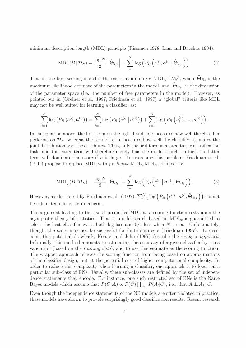
minimum description length (MDL) principle (Rissanen 1978; Lam and Bacchus 1994):
MDL(B | DN) =log N
2
∣∣∣ΘBS
∣∣∣− N∑i=1
log(PB
(c(i), a(i)
∣∣∣ ΘBS
)). (2)
That is, the best scoring model is the one that minimizes MDL(· | DN), where ΘBSis the
maximum likelihood estimate of the parameters in the model, and∣∣∣ΘBS
∣∣∣ is the dimension
of the parameter space (i.e., the number of free parameters in the model). However, aspointed out in (Greiner et al. 1997; Friedman et al. 1997) a “global” criteria like MDLmay not be well suited for learning a classifier, as:
N∑i=1
log(PB
(c(i), a(i)
))=
N∑i=1
log(PB
(c(i)∣∣a(i)
))+
N∑i=1
log(PB
(a
(i)1 , . . . , a(i)
n
)).
In the equation above, the first term on the right-hand side measures how well the classifierperforms on DN , whereas the second term measures how well the classifier estimates thejoint distribution over the attributes. Thus, only the first term is related to the classificationtask, and the latter term will therefore merely bias the model search; in fact, the latterterm will dominate the score if n is large. To overcome this problem, Friedman et al.(1997) propose to replace MDL with predictive MDL, MDLp, defined as:
MDLp(B | DN ) =log N
2
∣∣∣ΘBS
∣∣∣− N∑i=1
log(PB
(c(i)∣∣a(i) , ΘBS
)). (3)
However, as also noted by Friedman et al. (1997),∑N
i=1 log(PB
(c(i)∣∣∣a(i), ΘBS
))cannot
be calculated efficiently in general.
The argument leading to the use of predictive MDL as a scoring function rests upon theasymptotic theory of statistics. That is, model search based on MDLp is guaranteed toselect the best classifier w.r.t. both log-loss and 0/1-loss when N → ∞. Unfortunately,though, the score may not be successful for finite data sets (Friedman 1997). To over-come this potential drawback, Kohavi and John (1997) describe the wrapper approach.Informally, this method amounts to estimating the accuracy of a given classifier by crossvalidation (based on the training data), and to use this estimate as the scoring function.The wrapper approach relieves the scoring function from being based on approximationsof the classifier design, but at the potential cost of higher computational complexity. Inorder to reduce this complexity when learning a classifier, one approach is to focus on aparticular sub-class of BNs. Usually, these sub-classes are defined by the set of indepen-dence statements they encode. For instance, one such restricted set of BNs is the NaıveBayes models which assume that P (C|A) ∝ P (C)
∏ni=1 P (Ai|C), i.e., that Ai⊥⊥Aj |C.
Even though the independence statements of the NB models are often violated in practice,these models have shown to provide surprisingly good classification results. Resent research
4

into explaining the merits of the NB model has emphasized the difference between the 0/1-loss function and the log-loss, see e.g. (Friedman 1997; Domingos and Pazzani 1997).Friedman (1997, p. 76) concludes:
Good probability estimates are not necessary for good classification; similarly,low classification error does not imply that the corresponding class probabilitiesare being estimated (even remotely) accurately.
The starting point of Friedman (1997) is that a classifier learned for a particular do-main is a function of the training set. As the training set is considered a random samplefrom the domain, the classifier generated by a learner can be seen as a random variable;we shall use P (C = c |A) to denote the learned classifier. Friedman (1997) character-
izes a classifier based on its bias (i.e., EDN
[P (C |A)− P (C |A)
]2) and its variance (i.e.,
VarDN
(P (C |A)
)); the expectations are taken over all possible training sets of size N .
Friedman (1997) shows that in order to learn classifiers with low 0/1-loss it may not besufficient to simply focus on finding a model with low classifier bias; robustness in termsof low classifier variance can be just as important.
An example of a class of models where low bias (i.e., fairly high model expressibility) iscombined with robustness is the Tree Augmented Naıve Bayes (TAN) models, see (Fried-man et al. 1997). TAN models relax the NB assumption by allowing a more generalcorrelation structure between the attributes. More specifically, a Bayesian network modelis initially created over the variables in A, and this model is designed s.t. each variableAi has at most one parent (that is, the structure is a directed tree). Afterwards, the classattribute is included in the model by making it the parent of each attribute. Friedmanet al. (1997) use an adapted version of the algorithm by Chow and Liu (1968) to learnthe classifier, and they prove that the structure they find is the TAN which maximizes thelikelihood of DN ; the algorithm has time complexity O (n2(N + log(n))).
3 Hierarchical Naıve Bayes models
A special class of Bayesian networks is the so-called Hierarchical Naıve Bayes (HNB) mod-els, a concept first introduced by Zhang et al. (2002), see also (Zhang 2002; Kocka andZhang 2002). An HNB is a tree-shaped Bayesian network, where the variables are parti-tioned into three disjoint sets: C is the class variable, A is the set of attributes, and Lis a set of latent (or hidden) variables. In the following we use A to represent an attribute,whereas L is used to denote a latent variable; X and Y denote variables that may beeither attributes or latent variables. In an HNB the class variable C is the root of the tree(pa(C) = ∅) and the attributes are at the leaves (ch(A) = ∅, ∀A ∈ A); the latent variablesare all internal (ch (L) 6= ∅, pa (L) 6= ∅, ∀L ∈ L). The use of latent variables allows
5

conditional dependencies to be encoded in the model (as compared to e.g. the NB model).For instance, by introducing a latent variable as a parent of the attributes Ai and Aj , wecan represent the (local) dependence statement Ai 6⊥⊥Aj |C. Being able to model such localdependencies is particularly important for classification, as overlapping information wouldotherwise be double-counted. Note that the HNB model reduces to the NB model in thespecial case when there are no latent variables.
When learning an HNB we can restrict our attention to the parsimonious HNB models;we need not consider models which encode a probability distribution that is also encodedby another model which has fewer parameters. Formally, an HNB model, H = (BS, ΘBS
),with class variable C and attribute variables A is said to be parsimonious if there does notexist another HNB model, H ′ = (B′
S, Θ′BS
), with the same class and attribute variabless.t.:
i) H ′ has fewer parameters than H , i.e., |ΘBS| > |Θ′
BS|.
ii) The probability distributions over the class and attribute variables are the same inthe two models, i.e., P (C,A|BS, ΘBS
) = P (C,A|B′S, Θ′
BS).
In order to obtain an operational characterization of these models, Zhang et al. (2002)define the class of regular HNB models. An HNB model is said to be regular if for anylatent variable L, with neighbours (parent and children) X1, X2, . . .Xn, it holds that:
|sp(L)| ≤∏n
i=1 |sp(Xi)|maxi=1,...,n |sp(Xi)| ,
and strict inequality holds when L has only two neighbours and at least one of them is alatent node.
Zhang et al. (2002) show that i) any parsimonious HNB model is regular, and ii) for agiven set of class and attribute variables, the set of regular HNB model structures is finite.Observe that these two properties ensure that when searching for an HNB model we onlyneed to consider regular HNB models and we need not deal with infinite search spaces.
As opposed to other frameworks, such as NB or TAN models, an HNB can model anycorrelation among the attribute variables by simply choosing the state-spaces of the latentvariables large enough (although the encoding is not necessarily done in a cost-effectivemanner in terms of model complexity); note that the independence statements are notalways represented explicitly in the graphical structure, but are sometimes only encodedin the conditional probability tables. On the other hand, the TAN model, for instance,is particular efficient for encoding such statements but may fail to represent certain typesof dependence relations among the attribute variables. A TAN model is, e.g., not able torepresent the statement “C = 1 if and only if exactly two out of the three attributes A1,A2 and A3 are in state 1”.
6

4 Learning HNB classifiers
4.1 The main algorithm
Our search algorithm is based on a greedy search over the space of all HNBs; we initiate thesearch with an HNB model, H0, and learn a sequence Hk, k = 1, 2 . . . of HNB models.The search is conducted s.t. at each step we investigate the search boundary of the currentmodel (denoted B (Hk)), i.e., the set of models that can be reached from Hk in a singlestep. From this set of models the algorithm always selects a model with a higher scorethan the current one; if no such model can be found, then the current model is returned(see Algorithm 1).
Algorithm 1 (Greedy search)
1. Initiate model search with H0;
2. For k = 0, 1, . . .
(a) Select H ′ = arg maxH∈B(Hk)
Score(H | DN);
(b) If Score(H ′ | DN) > Score(Hk | DN) then:Hk+1 ← H ′; k ← k + 1;
elsereturn Hk;
In order to make the above algorithm operational we need to specify the score functionScore(· | DN) as well as the search operator (which again defines the search boundary).
The score-function is defined s.t. a high value corresponds to what is thought to be astructure with good classification qualities (as measured by the average loss on unseendata), i.e., Score(H | DN) measures the “goodness” of H . Note that the algorithm makessure that Score(Hk+1 | DN ) > Score(Hk | DN ) for k = 0, 1, . . . which ensures convergenceas long as the score is finite for all models. In order to apply a score metric that is closelyrelated to what the search algorithm tries to achieve, we use the wrapper approach byKohavi and John (1997). That is, we use cross validation (over the training set DN)to estimate an HNB’s classification accuracy on unseen data; notice that the test-set (ifdefined) is not used when the score is calculated.
The search operator is defined s.t. the HNB structure is grown incrementally. More specif-ically, if Lk is the set of latent variables in model Hk, then the set of latent variables inHk+1, is enlarged s.t. Lk+1 = Lk∪L, where L is a new latent variable. We restrict ourselfto only considering candidate latent variables which are parents of two variables X and Ywhere X, Y ⊆ ch (C) in Hk. Hence, we define Hk+1 as the HNB which is produced from
7
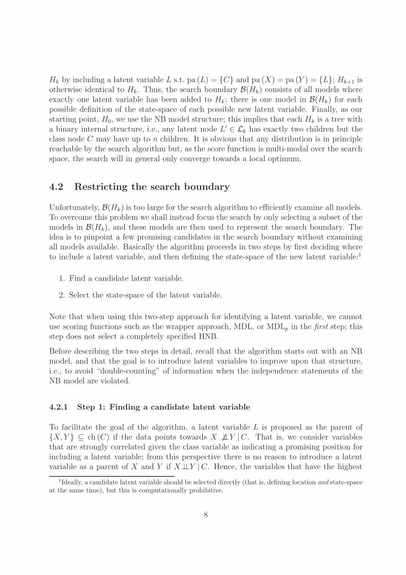
Hk by including a latent variable L s.t. pa (L) = C and pa (X) = pa (Y ) = L; Hk+1 isotherwise identical to Hk. Thus, the search boundary B(Hk) consists of all models whereexactly one latent variable has been added to Hk; there is one model in B(Hk) for eachpossible definition of the state-space of each possible new latent variable. Finally, as ourstarting point, H0, we use the NB model structure; this implies that each Hk is a tree witha binary internal structure, i.e., any latent node L′ ∈ Lk has exactly two children but theclass node C may have up to n children. It is obvious that any distribution is in principlereachable by the search algorithm but, as the score function is multi-modal over the searchspace, the search will in general only converge towards a local optimum.
4.2 Restricting the search boundary
Unfortunately, B(Hk) is too large for the search algorithm to efficiently examine all models.To overcome this problem we shall instead focus the search by only selecting a subset of themodels in B(Hk), and these models are then used to represent the search boundary. Theidea is to pinpoint a few promising candidates in the search boundary without examiningall models available. Basically the algorithm proceeds in two steps by first deciding whereto include a latent variable, and then defining the state-space of the new latent variable:1
1. Find a candidate latent variable.
2. Select the state-space of the latent variable.
Note that when using this two-step approach for identifying a latent variable, we cannotuse scoring functions such as the wrapper approach, MDL, or MDLp in the first step; thisstep does not select a completely specified HNB.
Before describing the two steps in detail, recall that the algorithm starts out with an NBmodel, and that the goal is to introduce latent variables to improve upon that structure,i.e., to avoid “double-counting” of information when the independence statements of theNB model are violated.
4.2.1 Step 1: Finding a candidate latent variable
To facilitate the goal of the algorithm, a latent variable L is proposed as the parent ofX, Y ⊆ ch (C) if the data points towards X 6⊥⊥Y |C. That is, we consider variablesthat are strongly correlated given the class variable as indicating a promising position forincluding a latent variable; from this perspective there is no reason to introduce a latentvariable as a parent of X and Y if X⊥⊥Y |C. Hence, the variables that have the highest
1Ideally, a candidate latent variable should be selected directly (that is, defining location and state-spaceat the same time), but this is computationally prohibitive.
8

correlation given the class variable may be regarded as the most promising candidate-pair. More specifically, we calculate the conditional mutual information given the classvariable, I(·, · |C), for all (unordered) pairs X, Y ⊆ ch (C). However, as I(X, Y |C)is increasing in both |sp (X)| and |sp (Y )| we cannot simply pick the pair X, Y thatmaximizes I(X, Y |C); this strategy would unintentionally bias the search towards latentvariables with children having large domains. Instead we utilize that:
2N · I(X, Y |C)L→ χ2∣∣∣sp (C)
∣∣∣(∣∣∣sp (X)∣∣∣−1
)(∣∣∣sp (Y )∣∣∣−1
),
whereL→ means convergence in distribution as N →∞, see e.g. (Whittaker 1990). Finally,
we calculateQ(X, Y | DN) = P (Z ≤ 2N · I(X, Y |C)) , (4)
where Z is χ2 distributed with |sp (C)| (|sp (X)| − 1) (|sp (Y )| − 1) degrees of freedom. Thepairs X, Y are ordered according to these probabilities, s.t. the pair with the highestprobability is picked out. By selecting the pairs of variables according to Q(X, Y | DN),the correlations are normalized w.r.t. the size differences in the state-spaces.
Unfortunately, to greedily select a pair of highly correlated variables as the children of anew latent variable is not always the same as improving classification accuracy, as can beseen from the example below:2
Example 1 Consider a classifier with binary attributes A = A1, A2, A3 (all with uni-form marginal distributions) and target concept C = 1 ⇔ A1 = 1 ∧ A2 = 1. Assumethat A1 and A2 are marginally independent but that P (A2 = A3) = 0.99. It then followsthat:
P (Q(A2, A3 | DN ) > Q(A1, A2 | DN ))→ 1
as N grows large (the uncertainty is due to the random nature of DN ). Hence, the heuristicwill not pick out A1, A2 which is most beneficial w.r.t.˙ classification accuracy, but willpropose to add a variable L′ with children ch (L′) = A2, A3.
4.2.2 Step 2: Selecting the state-space
To find the cardinality of a latent variable L, we use an algorithm similar to the oneby Elidan and Friedman (2001): Initially, the latent variable is defined s.t. |sp (L)| =∏
X∈ch(L) |sp (X)|, where each state of L corresponds to exactly one combination of thestates of the children of L. Let the states of the latent variable be labelled l1, . . . , lt.We then iteratively collapse two states li and lj into a single state l∗ as long as this is“beneficial”. Ideally, we would measure this benefit using the wrapper approach, but asthis is computationally expensive we shall instead use the MDLp score to approximate the
2This issue is also discussed in Section 6.
9

classification accuracy. Let H ′ = (B′S,ΘB′
S) be the HNB model obtained from a model
H = (BS,ΘBS) by collapsing states li and lj . Then li and lj should be collapsed if and only
if ∆L(li, lj | DN) = MDLp (H | DN) −MDLp (H ′ | DN) > 0. For each pair (li, lj) of stateswe therefore compute:
∆L(li, lj | DN ) = MDLp(H|DN )−MDLp(H′|DN)
=log(N)
2
(|ΘBS| − ∣∣ΘB′
S
∣∣)+ N∑i=1
[log(PH′(c(i)|a(i))
)− log(PH(c(i)|a(i))
)].
For the second term we first note that:
N∑i=1
[log(PH′(c(i)|a(i))
)− log(PH(c(i)|a(i))
)]=
N∑i=1
logPH′(c(i)|a(i))
PH(c(i)|a(i))
=∑
D∈DN :f(D,li,lj)
logPH′
(cD|aD
)PH (cD|aD)
,
where f(D, li, lj) is true if case D includes either L = li or L = lj; cases which does notinclude these states cancel out. This is also referred to as local decomposability in (Elidanand Friedman 2001), i.e., the gain of collapsing two states li and lj is local to those statesand it does not depend on whether or not other states have been collapsed. In order toavoid considering all possible combinations of the attributes we approximate the differencein predictive MDL as the difference w.r.t. the relevant subtree. The relevant subtree isdefined by C together with the subtree having L as root:3
∑D∈DN :f(D,li,lj)
logPH′
(cD|aD
)PH (cD|aD)
(5)
≈ log∏
c∈sp (C)
[(N(c, li)
N(li)
)N(c,li)
·(
N(c, lj)
N(lj)
)N(c,lj)
/
(N(c, li) + N(c, lj)
N(li) + N(lj)
)N(c,li)+N(c,lj)]
,
where N(c, s) and N(s) are the sufficient statistics, e.g., N(c, s) =∑N
i=1 γ(C = c, L = s :Di); γ(C = c, L = s : Di) takes on the value 1 if (C = c, L = s) appears in case Di, and0 otherwise; N(s) =
∑c∈sp (C) N(c, s). Note that Equation 5 is in fact an equality if the
relationship between C and ch (C) satisfy independence of causal influence (Heckermanand Breese 1994).
States are collapsed in a greedy manner, i.e., we find the pair of states with highest∆L(li, lj | DN ) and collapse those two states if ∆L(li, lj | DN) > 0. This is repeated (makinguse of local decomposability) until no states can be collapsed, see also Algorithm 2.
3The relevant subtree can also be seen as the part of the classifier structure that is directly affected bythe potential collapse of the states li and lj .
10
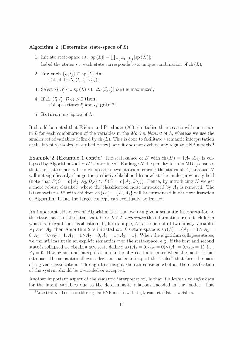
Algorithm 2 (Determine state-space of L)
1. Initiate state-space s.t. |sp (L)| = ∏X∈ch (L) |sp (X)|;
Label the states s.t. each state corresponds to a unique combination of ch (L);
2. For each li, lj ⊆ sp (L) do:Calculate ∆L(li, lj | DN);
3. Select l′i, l′j ⊆ sp (L) s.t. ∆L(l′i, l′j | DN) is maximized;
4. If ∆L(l′i, l′j | DN) > 0 then:
Collapse states l′i and l′j ; goto 2;
5. Return state-space of L.
It should be noted that Elidan and Friedman (2001) initialize their search with one statein L for each combination of the variables in the Markov blanket of L, whereas we use thesmaller set of variables defined by ch (L). This is done to facilitate a semantic interpretationof the latent variables (described below), and it does not exclude any regular HNB models.4
Example 2 (Example 1 cont’d) The state-space of L′ with ch (L′) = A2, A3 is col-lapsed by Algorithm 2 after L′ is introduced. For large N the penalty term in MDLp ensuresthat the state-space will be collapsed to two states mirroring the states of A2 because L′
will not significantly change the predictive likelihood from what the model previously held(note that P (C = c |A2, A3,DN ) ≈ P (C = c |A2,DN)). Hence, by introducing L′ we geta more robust classifier, where the classification noise introduced by A3 is removed. Thelatent variable L′′ with children ch (L′′) = L′, A1 will be introduced in the next iterationof Algorithm 1, and the target concept can eventually be learned.
An important side-effect of Algorithm 2 is that we can give a semantic interpretation tothe state-spaces of the latent variables: L ∈ L aggregates the information from its childrenwhich is relevant for classification. If, for example, L is the parent of two binary variablesA1 and A2, then Algorithm 2 is initiated s.t. L’s state-space is sp (L) = A1 = 0 ∧ A2 =0, A1 = 0∧A2 = 1, A1 = 1∧A2 = 0, A1 = 1∧A2 = 1. When the algorithm collapses states,we can still maintain an explicit semantics over the state-space, e.g., if the first and secondstate is collapsed we obtain a new state defined as (A1 = 0∧A2 = 0)∨(A1 = 0∧A2 = 1), i.e.,A1 = 0. Having such an interpretation can be of great importance when the model is putinto use: The semantics allows a decision maker to inspect the “rules” that form the basisof a given classification. Through this insight she can consider whether the classificationof the system should be overruled or accepted.
Another important aspect of the semantic interpretation, is that it allows us to infer datafor the latent variables due to the deterministic relations encoded in the model. This
4Note that we do not consider regular HNB models with singly connected latent variables.
11

fact provides us with a fast calculation scheme, as we “observe” all the variables in Aand L. Therefore, it also follows that we can represent the HNB classifier using only theclass variable and its children. Hence, the representation we will utilize is a Naıve Bayesstructure where the “attributes” are represented by the variables which occur as childrenof the class variable in the HNB model. It is simple to realize that the number of freeparameters required to represent this structure equals:
|ΘBS| = (|sp (C)| − 1) + |sp (C)|
∑X∈ch (C)
(|sp (X)| − 1) , (6)
see also (Kocka and Zhang 2002). Hence, the difference in predictive MDL (used in Algo-rithm 2) can be approximated by:
∆L(li, lj) ≈ log2(N)|sp (C)|
2(7)
−∑
c∈sp (C)
N(c, li) log2
(N(c, li)
N(c, li) + N(c, lj)
)
−∑
c∈sp (C)
N(c, lj) log2
(N(c, lj)
N(c, li) + N(c, lj)
)
+ N(li) log
(N(li)
N(li) + N(lj)
)+ N(lj) log
(N(lj)
N(li) + N(lj)
).
Note again that the approximation is exact if the relationship between C and the childrenof C can be modelled using independence of causal influence.
4.2.3 The search boundary
By following the two-step procedure described above, the focusing algorithm produces asingle candidate model H ′ ∈ B(Hk) to represent the search boundary. However, fromour experiments we have found that picking out a single model to represent the searchboundary is not an adequate representation of B(Hk). We can easily solve this drawbackin at least two different ways:
i) Go through the candidate latent nodes one at a time in order of decreasing Q(·, · | DN),and accept the first candidate model H ′′ ∈ B(Hk) for which Score(H ′′ | DN) >Score(Hk | DN ) in Step 2b of Algorithm 1.
ii) Limit the number of candidates used to represent the boundary to κ > 1 models,and do a greedy search over these models.
The first approach can be seen as a hill-climbing search, where we use Equation 4 to guidethe search in the right direction. Step 2a will in this case not be a maximization over
12
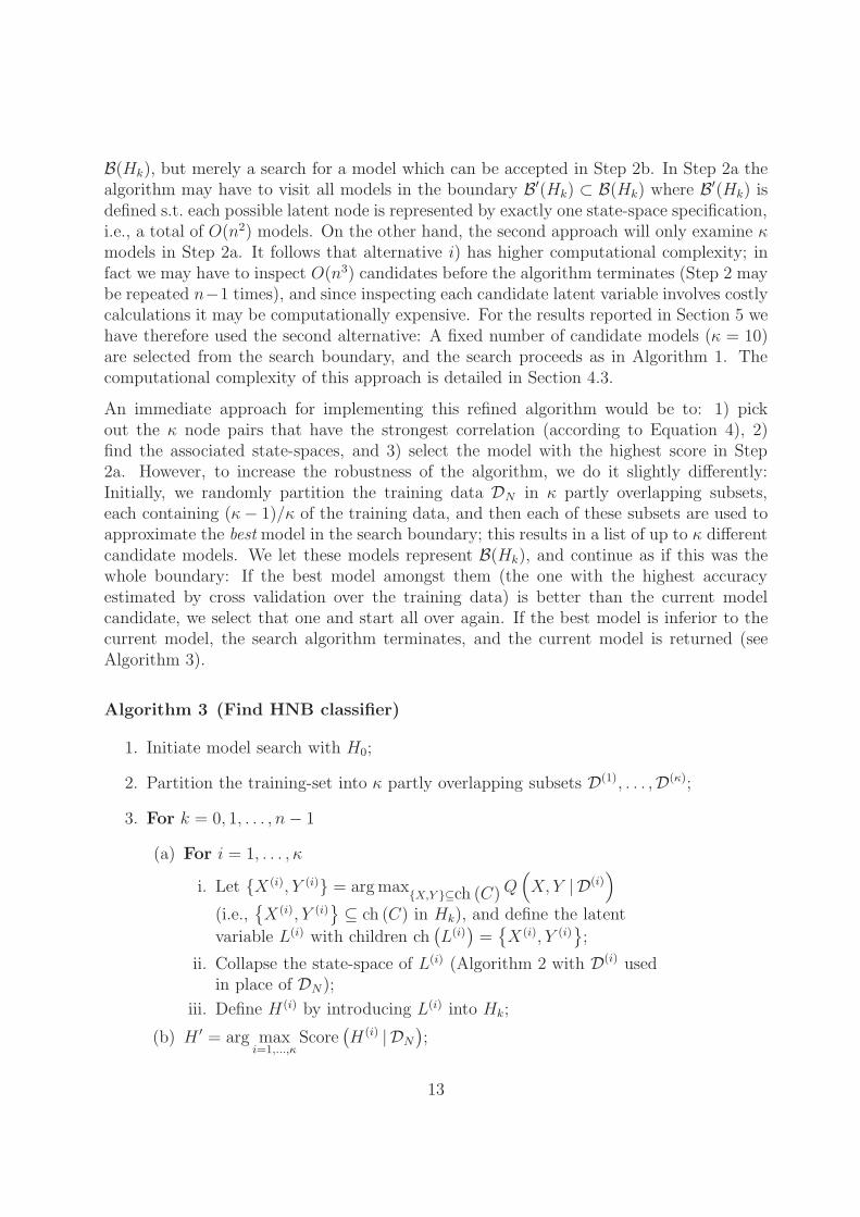
B(Hk), but merely a search for a model which can be accepted in Step 2b. In Step 2a thealgorithm may have to visit all models in the boundary B′(Hk) ⊂ B(Hk) where B′(Hk) isdefined s.t. each possible latent node is represented by exactly one state-space specification,i.e., a total of O(n2) models. On the other hand, the second approach will only examine κmodels in Step 2a. It follows that alternative i) has higher computational complexity; infact we may have to inspect O(n3) candidates before the algorithm terminates (Step 2 maybe repeated n−1 times), and since inspecting each candidate latent variable involves costlycalculations it may be computationally expensive. For the results reported in Section 5 wehave therefore used the second alternative: A fixed number of candidate models (κ = 10)are selected from the search boundary, and the search proceeds as in Algorithm 1. Thecomputational complexity of this approach is detailed in Section 4.3.
An immediate approach for implementing this refined algorithm would be to: 1) pickout the κ node pairs that have the strongest correlation (according to Equation 4), 2)find the associated state-spaces, and 3) select the model with the highest score in Step2a. However, to increase the robustness of the algorithm, we do it slightly differently:Initially, we randomly partition the training data DN in κ partly overlapping subsets,each containing (κ− 1)/κ of the training data, and then each of these subsets are used toapproximate the best model in the search boundary; this results in a list of up to κ differentcandidate models. We let these models represent B(Hk), and continue as if this was thewhole boundary: If the best model amongst them (the one with the highest accuracyestimated by cross validation over the training data) is better than the current modelcandidate, we select that one and start all over again. If the best model is inferior to thecurrent model, the search algorithm terminates, and the current model is returned (seeAlgorithm 3).
Algorithm 3 (Find HNB classifier)
1. Initiate model search with H0;
2. Partition the training-set into κ partly overlapping subsets D(1), . . . ,D(κ);
3. For k = 0, 1, . . . , n− 1
(a) For i = 1, . . . , κ
i. Let X(i), Y (i) = arg maxX,Y ⊆ch (C) Q(X, Y | D(i)
)(i.e.,
X(i), Y (i)
⊆ ch (C) in Hk), and define the latent
variable L(i) with children ch(L(i))
=X(i), Y (i)
;
ii. Collapse the state-space of L(i) (Algorithm 2 with D(i) usedin place of DN);
iii. Define H(i) by introducing L(i) into Hk;
(b) H ′ = arg maxi=1,...,κ
Score(H(i) | DN
);
13

(c) If Score(H ′ | DN) > Score(Hk | DN) then:Hk+1 ← H ′; k ← k + 1;
elsereturn Hk;
4. Return Hn;
4.3 Complexity analysis
When analyzing the complexity of the algorithm we can divide the description into threesteps:
1) Find a candidate latent variable.
2) Find the state-space of a candidate latent variable, and check if it is useful.
3) Iterate until no more candidate latent variables are accepted.
Part 1Proposing a candidate latent variable corresponds to finding the pair (X, Y ) of variableshaving the strongest correlation (Equation 4). There are at most (n2 − n)/2 such pairs,where n is the number of attribute variables. Calculating the conditional mutual informa-tion for a pair of variables can be done in time O(N) (N being the number of cases in thedatabase) hence, calculating the correlation measure for each pair of variables can be donein time O(N · n2). Finally, the list is sorted (to accommodate future iterations), and theresulting time complexity is O(n2 · (N + log(n))).
Part 2When determining the cardinality of a latent variable, L, we consider the gain of collaps-ing two states as compared to the current model; the gain is measured as the differencein predictive MDL. The time complexity of calculating the gain of collapsing two statesis simply O(N), see Equation 7. Due to local decomposability, the gain of collapsingtwo states has no effect on collapsing two other states, and there are therefore at most(|sp (L)|2 − |sp (L)|)/2 possible combinations, i.e., O(|sp (L)|2 · N). When two states arecollapsed, ∆L(·, ·) must be calculated for |sp (L)| − 1 new state combinations, next time|sp (L)|−2 state combinations are evaluated, and so on; the collapsing is performed at most|sp (L)| − 1 times. The time complexity of finding the state-space of a candidate latentvariable is therefore O
(N · |sp (L)|2 + N · |sp (L)| (|sp (L)| − 1)/2
)= O(|sp (L)|2 ·N).
Having found the cardinality of a candidate variable, say L, we test whether it shouldbe included in the model using the wrapper approach. From the rule-based propagationmethod it is easy to see that the time complexity of this task is O(n ·N). Thus, the timecomplexity of Part 2 is O((n + |sp (L)|2) ·N).
14

Part 3Each time a latent variable is introduced we would in principle need to perform the abovesteps again, and the time complexity would therefore be n− 1 times the time complexitiesabove. However, as described below some of the previous calculations can be reused.
First of all, as Q(X, Y |D) is a local measure we only need to calculate Q(L, Z|D), Z ∈ch (C), where L is the latent variable introduced in the previous iteration. Moreover, sincewe need to calculate Q(L, ·|D) at most n− 2 times, the time complexity will be O(n ·N),and, as the pairs (X, Y ) are still sorted according to Q(X, Y |D), we only need to sortn − 2 pairs, i.e., after having included a latent variable the re-initialization of step 1 hascomplexity O(n ·N + (n− 1) · log(n− 1)) = O(n · (N + log(n))).
Moreover, after having introduced a latent variable L with children X and Y , we cannotcreate another latent variable having either X or Y as a child (due to the structure of theHNB model). Thus, after having included a latent variable the cardinality of the resultingset of candidate pairs is reduced by n− 1. This implies that we will perform at most n− 2re-initializations, thereby giving the overall time complexity O(n2 ·N +n·(n·(N +log(n))+(|sp (L)|2 ·N))) = O(n2 · (log(n) + |sp (L)|2 ·N)).
5 Empirical results
In this section we will investigate the merits of the proposed learning algorithm by usingit to learn classifiers for a number of different domains. All data-sets are taken from theIrvine Machine Learning Repository (Blake and Merz 1998), see Table 1 for a summary ofthe 22 datasets used in this empirical study.
We have compared the results of the HNB classifier to those of the Naıve Bayes model(Duda and Hart 1973), the TAN model (Friedman et al. 1997), C5.0 (Quinlan 1998),and a standard implementation of neural networks with one hidden layer trained by back-propagation.5 As some of the learning algorithms require discrete variables, the attributeswere discretized using the entropy-based method of (Fayyad and Irani 1993). In addi-tion, instances containing missing attribute-values were removed; all pre-processing wasperformed using MLC++ (Kohavi et al. 1994).
The accuracy-results are given in Table 2. For each dataset we have estimated the accuracyof each classifier (in percentage of instances which are correctly classified), and give astandard deviation of this estimate. The standard deviations are the theoretical valuescalculated according to (Kohavi 1995), and are not necessarily the same as the empiricalstandard deviations observed during cross validation. For comparison of the algorithms
5We used Clementine (SPSS Inc. 2002) to generate the C5.0 and neural network models. We havenot compared our system to that of (Zhang et al. 2002) because of the high computational complexity ofZhang et al.’s algorithm. However, the numerical results reported by Zhang et al. (2002) point towardsour model offering significantly better classification accuracy.
15

#Inst #InstDatabase #Att #Cls Train Test Database #Att #Cls Train Testpostop 8 3 90 CV(5) cleve 13 2 296 CV(5)iris 4 3 150 CV(5) wine 13 3 178 CV(5)monks-1 6 2 124 432 thyroid 5 3 215 CV(5)monks-2 6 2 124 432 ecoli 7 8 336 CV(5)monks-3 6 2 124 432 breast 10 2 683 CV(5)glass 9 7 214 CV(5) vote 16 2 435 CV(5)glass2 9 2 163 CV(5) crx 15 2 653 CV(5)diabetes 8 2 768 CV(5) australian 14 2 690 CV(5)heart 13 2 270 CV(5) chess 36 2 2130 1066hepatitis 19 2 155 CV(5) vehicle 18 4 846 CV(5)pima 8 2 768 CV(5) soybean-large 35 19 562 CV(5)
Table 1: A summary of the 22 databases used in the experiments: #Att indicates thenumber of attributes; #Cls is the number of classes; #Inst is the number of instances(given separately for training and test sets). CV(5) denotes 5-fold cross validation. Furtherdetails regarding the datasets can be found at the UCI Machine Learning Repository.
we made sure that the same cross validation folds were used for all the different learningmethods. The best result for each dataset is given in boldface. We note that the HNBclassifier achieves the best result for 10 of the 22 datasets, comes top-two for all but 5datasets, and also has the best performance averaged over all datasets.
To quantify the difference between the HNB classifier and the other classifiers we advocatethe method of (Kohavi 1995); Kohavi (1995) argues that the true merit of a classifiercannot be found by calculating the accuracy on a finite test-set. Instead we define α as thetrue accuracy of a classifier (only to be found if the target concept of the domain is knownor fully described by an infinite test set), and we use α to denote the estimate of α basedon a test set of size N . Kohavi (1995) argues that α is approximately Gaussian distributedwith expectation α and variance α · (1− α)/N for large N . In our setting we have severaldatasets (indexed by i = 1, . . . , t; t is the number of datasets, i.e., t = 22 in this study) andseveral classifier algorithms (indexed by j), and with this notation Kohavi’s approximationcan be written as αij ∼ N (αij, αij · (1 − αij)/Ni). To simplify, we assume αij⊥⊥αik forj 6= k and αij⊥⊥α`j for i 6= `. Finally, we use the estimated standard deviation sij (givenin Table 2) as if it was known. It follows that under the hypothesis that classifiers j andk are equally capable (αij = αik, i = 1, . . . , t) then:
Λi(j, k) = αij − αik ∼ N (0, s2ij + s2
ik) , Λ(j, k) =t∑
i=1
Λi
t∼ N
(0,
t∑i=1
s2ij + s2
ik
t2
).
This enables us to test the hypothesis that the HNB classifier is not better than the otherclassifiers; more precisely we test the hypothesis H0: Λ(·, ·) ≤ 0 against H1: Λ(·, ·) > 0,
16
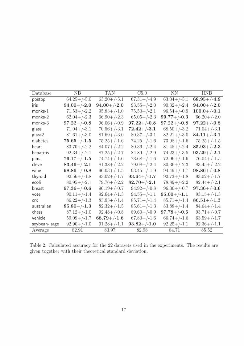
Database NB TAN C5.0 NN HNBpostop 64.25+/-5.0 63.20+/-5.1 67.31+/-4.9 63.04+/-5.1 68.95+/-4.9iris 94.00+/-2.0 94.00+/-2.0 93.55+/-2.0 90.32+/-2.4 94.00+/-2.0monks-1 71.53+/-2.2 95.83+/-1.0 75.50+/-2.1 96.54+/-0.9 100.0+/-0.1monks-2 62.04+/-2.3 66.90+/-2.3 65.05+/-2.3 99.77+/-0.3 66.20+/-2.0monks-3 97.22+/-0.8 96.06+/-0.9 97.22+/-0.8 97.22+/-0.8 97.22+/-0.8glass 71.04+/-3.1 70.56+/-3.1 72.42+/-3.1 68.50+/-3.2 71.04+/-3.1glass2 81.61+/-3.0 81.69+/-3.0 80.37+/-3.1 82.21+/-3.0 84.11+/-3.1diabetes 75.65+/-1.5 75.25+/-1.6 74.25+/-1.6 73.08+/-1.6 75.25+/-1.5heart 83.70+/-2.2 84.07+/-2.2 80.36+/-2.4 81.45+/-2.4 85.93+/-2.3hepatitis 92.34+/-2.1 87.25+/-2.7 84.89+/-2.9 74.23+/-3.5 93.29+/-2.1pima 76.17+/-1.5 74.74+/-1.6 73.68+/-1.6 72.96+/-1.6 76.04+/-1.5cleve 83.46+/-2.1 81.38+/-2.2 79.08+/-2.4 80.36+/-2.3 83.45+/-2.2wine 98.86+/-0.8 96.03+/-1.5 93.45+/-1.9 94.49+/-1.7 98.86+/-0.8thyroid 92.56+/-1.8 93.02+/-1.7 93.64+/-1.7 92.73+/-1.8 93.02+/-1.7ecoli 80.95+/-2.1 79.76+/-2.2 82.70+/-2.1 78.89+/-2.2 82.44+/-2.1breast 97.36+/-0.6 96.19+/-0.7 94.92+/-0.8 96.36+/-0.7 97.36+/-0.6vote 90.11+/-1.4 92.64+/-1.3 94.55+/-1.1 95.00+/-1.1 93.15+/-1.3crx 86.22+/-1.3 83.93+/-1.4 85.71+/-1.4 85.71+/-1.4 86.51+/-1.3australian 85.80+/-1.3 82.32+/-1.5 85.61+/-1.3 83.88+/-1.4 84.64+/-1.4chess 87.12+/-1.0 92.48+/-0.8 89.60+/-0.9 97.78+/-0.5 93.71+/-0.7vehicle 59.09+/-1.7 68.79+/-1.6 67.80+/-1.6 66.74+/-1.6 63.59+/-1.7soybean-large 92.90+/-1.0 91.28+/-1.1 93.82+/-1.0 92.25+/-1.1 92.36+/-1.1Average 82.91 83.97 82.98 84.71 85.52
Table 2: Calculated accuracy for the 22 datasets used in the experiments. The results aregiven together with their theoretical standard deviation.
17

05
1015202530354045
0 5 10 15 20 25 30 35 40 45
HN
B c
lass
ifica
tion
erro
r
NB classification error
05
1015202530354045
0 5 10 15 20 25 30 35 40 45
HN
B c
lass
ifica
tion
erro
r
TAN classification error
a) NB vs. HNB b) TAN vs. HNB
05
1015202530354045
0 5 10 15 20 25 30 35 40 45
HN
B c
lass
ifica
tion
erro
r
C5.0 classification error
05
1015202530354045
0 5 10 15 20 25 30 35 40 45
HN
B c
lass
ifica
tion
erro
r
NN classification error
c) C5.0 vs. HNB d) NN vs. HNB
Figure 2: Scatter plot of classification error for HNB and a selection of other classificationsystems. In each plot, a point represents a dataset. The HNB’s classification error is givenon the x-axis, whereas the other system’s error is given on the y-axis. Hence, data pointsbelow the diagonal corresponds to datasets where the HNB is superior, whereas pointsabove the diagonal are datasets where the HNB classifier is inferior to the other system.
where the classifiers are labelled s.t. higher average accuracy for the HNB classifier coincideswith a positive value of Λ(·, ·). With this setup H0 is rejected at level p = 5 · 10−12 (NB),p = 6 · 10−6 (TAN), p = 6 · 10−11 (C5.0) and p = .02 (NN).
Finally, we note that in some of the domains the HNB models come up with an interestinglatent structure. We are not experts to tell whether these structures are in fact meaningful,but some of them are at least worth attention. For example, in the heart model the HNBaggregates information about “Chest pain” and “Training induced angina”. The probabil-ity of a heart disease increases slightly when chest pain is of a certain type; this probabilitycan then again be increased dramatically if the instance also contains information about atraining induced angina. Training induced angina has no effect in the model if chest pain isnot of this particular type. Note that the classifier in this example uses the latent variableto encode context specific independence (Boutilier et al. 1996).
18

6 Discussion
6.1 Parameter learning
The parameters in the model are estimated by their maximum likelihood values. Thismay not be optimal for classification, and recent research has shown some improvementin classification accuracy when the parameters are chosen otherwise (Wettig et al. 2002).However, to support the interpretation of the empirical results in Section 5 we have delib-erately not taken the opportunity of improving the classification accuracy further in thisway. Optimization of the model is left for future work.
6.2 Finding candidate latent variables
As described by Example 1 and Example 2 the search for candidate latent variables mayintroduce a latent variable for a pair of variables which are marginally dependent, but whereonly one of the variables is actually dependent on the class variable C; as also shown isthe examples, this does not jeopardize classification accuracy (actually it can be seen asa form of feature selection). Similarly, if several attributes are marginally dependent butindependent of the class variable, the algorithm performs some redundant computations:For each such pair of attributes we include a latent variable, but as these attributes areindependent of the class variable all states of such a latent variable are collapsed and theeffect of the attributes on the classification result is removed.
Obviously both of the above mentioned problems can be overcome by simply performinga feature selection before initializing the learning algorithm. However, another approachwould be to apply a correlation measure which directly considers the probability distribu-tion over the class variable conditioned on the two variables X and Y in question. That is,the difference between the probability distribution P (C|X, Y ) and the probability distribu-tion P ′(C|X, Y ), where the latter is encoded by the model where X⊥⊥Y |C. This distancecan be described using the well-known Kullback-Leibler (KL) divergence (Kullback andLeibler 1951) averaged over the possible states of X and Y :
E(KL(P ; P ′)|X, Y ) =∑x,y
P (x, y)∑
c
P (c|x, y) log
(P (c|x, y)
P ′(c|x, y)
).
In the context of classification, this distance measure can also be given another interpre-
19
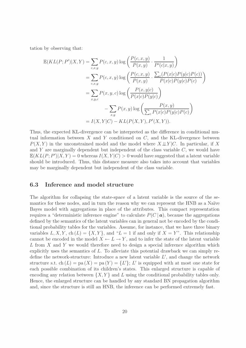
tation by observing that:
E(KL(P ; P ′)|X, Y ) =∑c,x,y
P (c, x, y) log
(P (c, x, y)
P (x, y)· 1
P ′(c|x, y)
)
=∑c,x,y
P (c, x, y) log
(P (c, x, y)
P (x, y)·∑
c(P (x|c)P (y|c)P (c))
P (x|c)P (y|c)P (c)
)
=∑x,y,c
P (x, y, c) log
(P (x, y|c)
P (x|c)P (y|c))
−∑x,y
P (x, y) log
(P (x, y)∑
c P (x|c)P (y|c)P (c)
)
= I(X, Y |C)−KL(P (X, Y ), P ′(X, Y )).
Thus, the expected KL-divergence can be interpreted as the difference in conditional mu-tual information between X and Y conditioned on C, and the KL-divergence betweenP (X, Y ) in the unconstrained model and the model where X⊥⊥Y |C. In particular, if Xand Y are marginally dependent but independent of the class variable C, we would haveE(KL(P ; P ′)|X, Y ) = 0 whereas I(X, Y |C) > 0 would have suggested that a latent variableshould be introduced. Thus, this distance measure also takes into account that variablesmay be marginally dependent but independent of the class variable.
6.3 Inference and model structure
The algorithm for collapsing the state-space of a latent variable is the source of the se-mantics for these nodes, and in turn the reason why we can represent the HNB as a NaıveBayes model with aggregations in place of the attributes. This compact representationrequires a “deterministic inference engine” to calculate P (C |a), because the aggregationsdefined by the semantics of the latent variables can in general not be encoded by the condi-tional probability tables for the variables. Assume, for instance, that we have three binaryvariables L, X, Y , ch (L) = X, Y , and “L = 1 if and only if X = Y ”. This relationshipcannot be encoded in the model X ← L→ Y , and to infer the state of the latent variableL from X and Y we would therefore need to design a special inference algorithm whichexplicitly uses the semantics of L. To alleviate this potential drawback we can simply re-define the network-structure: Introduce a new latent variable L′, and change the networkstructure s.t. ch (L) = pa (X) = pa (Y ) = L′; L′ is equipped with at most one state foreach possible combination of its children’s states. This enlarged structure is capable ofencoding any relation between X, Y and L using the conditional probability tables only.Hence, the enlarged structure can be handled by any standard BN propagation algorithmand, since the structure is still an HNB, the inference can be performed extremely fast.
20

7 Concluding remarks
In this paper we have used Hierarchical Naıve Bayes models for classification, and throughexperiments we have shown that the HNB classifiers offer results that are significantlybetter than those of other commonly used classification methods. Moreover, a numberof existing tools may be able to improve the classification accuracy even further. Theseinclude feature selection (Kohavi and John 1997), smoothing (significant improvementsreported by (Friedman et al. 1997) for some model classes), and supervised learning of theprobability parameters (Wettig et al. 2002). We leave the investigation of these sourcesof potential improvements for future work. Finally, the proposed learning algorithm alsoprovides an explicit semantics for the latent structure of a model. This allows a decisionmaker to easily deduce the rules which govern the classification of some instance hence,the semantics may also increase the user’s confidence in the model.
Acknowledgements
We have benefited from interesting discussions with the members of the Decision SupportSystems group at Aalborg University, in particular Tomas Kocka, Nevin L. Zhang, andJirı Vomlel. We would like to thank Hugin Expert (www.hugin.com) for giving us accessto Hugin Decision Engine which forms the basis for our implementation. The first authorwas supported by a grant from the Research Council of Norway.
References
Blake, C. and C. Merz (1998). UCI repository of machine learning databases. URL:http://www.ics.uci.edu/∼mlearn/MLRepository.html.
Boutilier, C., N. Friedman, M. Goldszmidt, and D. Koller (1996). Context-specific inde-pendence in Bayesian networks. In Proceedings of the Twelfth Annual Conference onUncertainty in Artificial Intelligence, Portland, OR., pp. 115–123.
Chow, C. K. and C. Liu (1968). Approximating discrete probability distributions withdependence trees. IEEE Transactions on Information Theory 14, 462–467.
Cowell, R. G., A. P. Dawid, S. L. Lauritzen, and D. J. Spiegelhalter (1999). ProbabilisticNetworks and Expert Systems. Statistics for Engineering and Information Sciences.New York: Springer Verlag.
Domingos, P. and M. Pazzani (1997). On the optimality of the simple Bayesian classifierunder zero-one loss. Machine Learning 29 (2–3), 103–130.
Duda, R. O. and P. E. Hart (1973). Pattern Classification and Scene Analysis. NewYork: John Wiley & Sons.
21
Elidan, G. and N. Friedman (2001). Learning the dimensionality of hidden variables. InProceedings of the Seventeenth Conference on Uncertainty in Artificial Intelligence,San Francisco, CA., pp. 144–151. Morgan Kaufmann Publishers.
Fayyad, U. M. and K. B. Irani (1993). Multi-interval discretization of continuous-valuedattributes for classification learning. In Proceedings of the Thirteenth InternationalJoint Conference on Artificial Intelligence, San Mateo, CA., pp. 1022–1027. MorganKaufmann Publishers.
Friedman, J. H. (1997). On bias, variance, 0/1-loss, and the curse of dimensionality.Data Mining and Knowledge Discovery 1 (1), 55–77.
Friedman, N., D. Geiger, and M. Goldszmidt (1997). Bayesian network classifiers. Ma-chine Learning 29 (2–3), 131–163.
Greiner, R., A. J. Grove, and D. Schuurmans (1997). Learning Bayesian nets that per-form well. In Proceedings of the Thirteenth Annual Conference on Uncertainty inArtificial Intelligence, San Francisco, CA., pp. 198–207. Morgan Kaufmann Publish-ers.
Heckerman, D. and J. S. Breese (1994). A new look at causal independence. In Proceed-ings of the Tenth Annual Conference on Uncertainty in Artificial Intelligence, SanFrancisco, CA., pp. 286–292. Morgan Kaufmann Publishers.
Jensen, F. V. (2001). Bayesian Networks and Decision Graphs. New York: SpringerVerlag.
Kohavi, R. (1995). A study of cross-validation and bootstrap for accuracy estimationand model selection. In Proceedings of the Fourteenth International Joint Confer-ence on Artificial Intelligence, San Mateo, CA., pp. 1137–1143. Morgan KaufmannPublishers.
Kohavi, R., G. John, R. Long, D. Manley, and K. Pfleger (1994). MLC++: A machinelearning library in C++. In Proceedings of the Sixth International Conference onTools with Artificial Intelligence, pp. 740–743. IEEE Computer Society Press.
Kohavi, R. and G. H. John (1997). Wrappers for feature subset selection. ArtificialIntelligence 97 (1–2), 273–324.
Kononenko, I. (1991). Semi-naive Bayesian classifier. In Proceedings of Sixth EuropeanWorking Session on Learning, Berlin. Springer Verlag.
Kocka, T. and N. L. Zhang (2002). Dimension correction for hierarchical latent classmodels. In Proceedings of the Eighteenth Conference on Uncertainty in ArtificialIntelligence, San Francisco, CA., pp. 267–274. Morgan Kaufmann Publishers.
Kullback, S. and R. A. Leibler (1951). On information and sufficiency. Annals of Math-ematical Statistics 22, 79–86.
Lam, W. and F. Bacchus (1994). Learning Bayesian belief networks: An approach basedon the MDL principle. Computational Intelligence 10 (4), 269–293.
22
Mitchell, T. M. (1997). Machine Learning. Boston, MA.: McGraw Hill.
Pazzani, M. (1995). Searching for dependencies in Bayesian classifiers. In Proceedings ofthe Fifth International Workshop on Artificial Intelligence and Statistics.
Pearl, J. (1988). Probabilistic Reasoning in Intelligent Systems: Networks of PlausibleInference. San Mateo, CA.: Morgan Kaufmann Publishers.
Quinlan, R. (1998). C5.0: An informal tutorial. Available from the internet at URL:http://www.rulequest.com/see5-unix.html.
Rissanen, J. (1978). Modelling by shortest data description. Automatica 14, 465–471.
Schwarz, G. (1978). Estimating the dimension of a model. Annals of Statistics 6, 461–464.
SPSS Inc. (2002). Clementine v6.5. http://www.spss.com/spssbi/clementine/index.htm.
Wettig, H., P. Grunwald, T. Roos, P. Myllymaki, and H. Tirri (2002). On supervisedlearning of Bayesian network parameters. HIIT Technical Report 2002-1, HelsinkiInstitute for Information Technology.
Whittaker, J. (1990). Graphical models in applied multivariate statistics. Chichester:John Wiley & Sons.
Zhang, N. (2002). Hierarchical latent class models for cluster analysis. In Proceedings ofthe Eighteenth National Conference on Artificial Intelligence, Menlo Park, CA., pp.230–237. AAAI Press.
Zhang, N., T. D. Nielsen, and F. V. Jensen (2002). Latent variable discovery in classifi-cation models. Available from the first author upon request.
23


IV
Parameter Learning in Object Oriented Bayesian Networks


Annals of Mathematics and Artificial Intelligence 32: 221–243, 2001. 2001 Kluwer Academic Publishers. Printed in the Netherlands.
Parameter learning in object-oriented Bayesian networks
Helge Langseth a,b and Olav Bangsø b
a Department of Mathematical Sciences, Norwegian University of Science and Technology, N-7491Trondheim, Norway
E-mail: [email protected] Department of Computer Science, Aalborg University, Fredrik Bajers Vej 7E,
DK-9220 Aalborg Øst, DenmarkE-mail: hl, [email protected]
This paper describes a method for parameter learning in Object-Oriented Bayesian Net-works (OOBNs). We propose a methodology for learning parameters in OOBNs, and provethat maintaining the object orientation imposed by the prior model will increase the learn-ing speed in object-oriented domains. We also propose a method to efficiently estimate theprobability parameters in domains that are not strictly object oriented. Finally, we attack typeuncertainty, a special case of model uncertainty typical to object-oriented domains.
Keywords: Bayesian networks, object orientation, learning
AMS subject classification: 68T05
1. Introduction
Bayesian Networks (BNs) [21,32] have established themselves as a powerful toolin many areas of artificial intelligence, including planning, vision, decision support sys-tems and robotics. However, one of the main obstacles is to create and maintain verylarge domain models. To remedy this problem, object-oriented versions of the BN frame-work have been proposed in the literature [4,22]. Object-Oriented BNs (OOBNs) as de-fined in these papers offer an easy way of creating BNs, but the problem of assessingand maintaining the probability estimates still remain; conventional learning algorithmslike [6] do not exploit that the domain is object oriented while learning.
In this paper we propose a learning method that is applied directly to the OOBNspecification. It is proven that this learning method is superior to conventional learningmethods in object oriented domains, and a method to efficiently estimate the probabilityparameters in domains that are not strictly object oriented is also proposed.
This paper is organized as follows: The rest of this section will create a startingpoint for our analysis by introducing OOBNs and the required notation and assump-tions. In section 2 we outline the proposed learning method, and in section 3 we pro-pose a framework for learning in domains that are only approximately object oriented.A special case of model uncertainty, typical to object-oriented domains, is handled insection 4, and we conclude in section 5.

222 H. Langseth, O. Bangsø / Parameter learning in OOBNs
1.1. Object-oriented Bayesian networks
Using small and “easy-to-read” pieces of a complex model is an already appliedtechnique for constructing large Bayesian networks. For instance, [34] introduces theconcept of sub-networks which can be viewed and edited separately even if they are dif-ferent pieces of the same network; [37] adds levels of integration of fragments (using ananalogy with Boolean circuits); [25] is concerned with the combination of fragments(using conditional noisy-MIN). Frameworks for such representations called Object-Oriented Bayesian Networks are presented in [4,22]. An introduction to the frameworkof [4] will be given in this section, as it is the foundation for our work on learning inOOBNs.
OOBNs as defined by [4] will be described in the following by way of an exampleadapted from that paper. The example will be used throughout the paper to illustrate theproposed learning mechanism and to show how well it works. We limit our descriptionof the framework to those parts that are most relevant for learning in OOBNs; furtherdetails can be found in [3,4]. This font will be used to describe classes, instantiationsof classes are described using THIS FONT, and this font is employed when referring tovariables.
Old McDonald (OMD) has a farm with 2 milk cows and 2 meat cows. A milk cowprimarily produces milk and a meat cow primarily produces meat. OMD wants to modelhis stock using OOBN classes. OMD constructs a Generic cow as shown in figure 1. Heknows that what a cow eats and who its mother is influences how much milk and meat itproduces. OMD wants Mother and Food to be input nodes; an input node is a referenceto a node outside the class. OMD wants Milk and Meat to be output nodes, nodes froma class usable outside the instantiations of the class. Dashed ellipses represent inputnodes and shaded ellipses represent output nodes, see figure 1. Input and output nodesform the interface between an instantiation and the context in which the instantiation ex-ists. Nodes in an instantiation that are neither input nor output nodes are termed normalnodes. A class may be instantiated several times with different nodes having influenceon the different instantiations through the input nodes, so only the number of states ofthe input nodes is known at the time of specification (e.g., the cows might have differentmothers).
Figure 1. The Generic cow class as defined by OMD. The arrows are links as in normal BNs. The dashedellipses are input nodes, and the shaded ellipses are output nodes.

H. Langseth, O. Bangsø / Parameter learning in OOBNs 223
OMD consults an expert that tells him that he might want to get specifications ofboth a Milk cow and a Meat cow, which OMD agrees to. The two new cow specifi-cations, shown in figure 2, are subclasses of the Generic cow class (hence the “IS AGeneric cow” in the top left of each of the class specifications). A class S can be a sub-class of another class C if S contains at least the same set of nodes as C. This ensures thatan instantiation of S can be used anywhere in the OOBN instead of an instantiation of C(e.g., an instantiation of Milk cow can be used instead of an instantiation of Genericcow). Each node in a subclass inherits the conditional probability tables (CPTs) of thecorresponding node in its superclass unless the parent sets differ, or the modeler explic-itly overwrites the CPT. The sub–superclass relation is transitive but not antisymmetric,so to avoid cycles it is required that a subclass of a class cannot be a superclass of thisclass as well. Furthermore, multiple inheritance is not allowed, so the structure of theclass hierarchy will be a tree or a collection of disjoint trees called a forest. All treesfrom the class hierarchy forest can be arranged so that the unique node with no super-class is the root, and all other nodes of the tree have their superclass as parent. Such atree is called a class tree.
OMD continues by constructing a Stock class representing his live-stock. In fig-ure 3 the boxes are instantiations, e.g., Cow1 is an instantiation of the class Meat cow.
(a) (b)
Figure 2. (a) The experts specification of a Milk cow. (b) The experts specification of a Meat cow. Notethat their input sets are larger than the input set of the Generic cow (figure 1).
Figure 3. The Stock with two instantiations of the Milk cow class and two instantiations of the Meat cowclass. Note that some input nodes are not referencing any nodes.

224 H. Langseth, O. Bangsø / Parameter learning in OOBNs
This is indicated by Cow1:Meat cow inside the Cow1 instantiation. Note that only inputnodes and output nodes are visible, as they are the only part of the instantiation availableto the encapsulating class (Stock). The double arrows are reference links, where the leafof a link is a reference to the root of that link;1 e.g., the input node Mother of Cow1 isa reference to the node Daisy. This means that whenever the node Mother is to be usedinside the instantiation Cow1, the node Daisy will be the node actually used.
As the subclasses in a class tree may have a larger set of nodes than their superclass,the input set of a subclass S might be larger than the input set of its superclass C. If aninstantiation of S is used instead of an instantiation of C, the extra input nodes will not bereferencing a node. To ensure that these nodes contain a potential, the notion of a defaultpotential is introduced: a default potential is a probability distribution over the states ofan input node, which is used when the input node is not referencing any node. A defaultpotential can also be used when no reference link is specified, even if the reason for it isnot subclassing. Not all the Mother nodes in figure 3 reference a node, but because ofthe default potential all nodes are still associated with a CPT. It is also worth noting thatthe structure of references is always a tree or a forest; cycles of reference links are notpossible [3]. These trees consist of a unique root and one or more leaf-nodes; there areonly two “layers” in these structures in our case.
Inference can be performed by translating the OOBN into a multiply-sectionedBayesian network [41,42], see [3] for details on this translation, or by constructing theunderlying BN. The underlying BN, BNI, of an instantiation I is constructed using thefollowing algorithm, assuming I to define a legal OOBN:
1. Let BNI be the empty graph.
2. Add a node to BNI for all input nodes, output nodes and normal nodes in I.
3. Add a node to BNI for each input node, output node and normal node of the instan-tiations contained in I, and prefix the name of the instantiation to the node name(Instantiation-name.Node-name). Do the same for instantiations contained in theseinstantiations, and so on.
4. Add a link for each normal link in I, and repeat this for all instantiations as above.
5. For each reference tree, merge all the nodes into one node. This node is given all theparents and children (according to the normal links) of the nodes in the reference treeas its family. Note that only the root of the tree can have parents, as all other nodesare references to this node.
An input node that does not reference another node will become a normal nodeequipped with the default potential. Figure 4 describes the underlying BN of OMD’sinstantiation of the Stock-class (figure 3) as found by the above algorithm.
1 To avoid confusion with the normal links in the model we do not use the terms “parent” and “child” whenreferring to reference links.
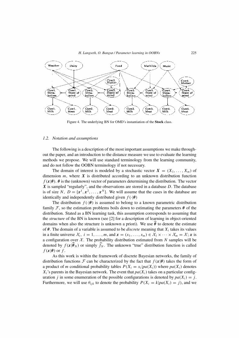
H. Langseth, O. Bangsø / Parameter learning in OOBNs 225
Figure 4. The underlying BN for OMD’s instantiation of the Stock class.
1.2. Notation and assumptions
The following is a description of the most important assumptions we make through-out the paper, and an introduction to the distance measure we use to evaluate the learningmethods we propose. We will use standard terminology from the learning community,and do not follow the OOBN terminology if not necessary.
The domain of interest is modeled by a stochastic vector X = (X1, . . . , Xm) ofdimension m, where X is distributed according to an unknown distribution functionf (x|θ). θ is the (unknown) vector of parameters determining the distribution. The vectorX is sampled “regularly”, and the observations are stored in a database D. The databaseis of size N, D = x1, x2, . . . , xN . We will assume that the cases in the database areidentically and independently distributed given f (·|θ)
The distribution f (·|θ) is assumed to belong to a known parametric distributionfamily F , so the estimation problems boils down to estimating the parameters θ of thedistribution. Stated as a BN learning task, this assumption corresponds to assuming thatthe structure of the BN is known (see [2] for a description of learning in object-orienteddomains when also the structure is unknown a priori). We use θ to denote the estimateof θ . The domain of a variable is assumed to be discrete meaning that Xi takes its valuesin a finite universe Xi , i = 1, . . . , m, and x = (x1, . . . , xm) ∈ X1× · · · ×Xm = X ; x isa configuration over X . The probability distribution estimated from N samples will bedenoted by f (x |θN) or simply fN . The unknown “true” distribution function is calledf (x|θ) or f .
As this work is within the framework of discrete Bayesian networks, the family ofdistribution functions F can be characterized by the fact that f (x|θ) takes the form ofa product of m conditional probability tables P(Xi = xi |pa(Xi)) where pa(Xi) denotesXi’s parents in the Bayesian network. The event that pa(Xi) takes on a particular config-uration j in some enumeration of the possible configurations is denoted by pa(Xi) = j .Furthermore, we will use θijk to denote the probability P(Xi = k|pa(Xi) = j), and we

226 H. Langseth, O. Bangsø / Parameter learning in OOBNs
will assume 0 < θijk < 1 to avoid trivial deterministic cases of learning.2 We will let |θ |denote the dimension of the parameter space, meaning the smallest possible number offree parameters that can encode f (x|θ) correctly. This is not the same as the sum of thesizes of the CPTs, since one can, e.g., encode the distribution of a binary variable X byusing only the one parameter p, i.e., P(X = 1) = p, P (X = 0) = 1 − P(X = 1) =1−p. |θ | is, furthermore, not to be calculated directly from the dimension of X , since aBayesian network (that is not a complete graph) utilizes a more compact representation.
The work presented in this paper focuses on the maximum likelihood estimatesof the parameters. To generate the maximum likelihood estimates we use the EM-algorithm [12]. The EM-algorithm is particularly easy to implement in graphical mod-els [26], but there are problematic issues both regarding speed of convergence as well asconvergence towards a local (sub-optimal) maximum of the likelihood function. The firstof these problems can be overcome by different acceleration measures, see, e.g., [31,38],the second problem is typically managed by a series of random restarts of the iterationprocess after convergence of the EM algorithm.
The work described here does not consider the use of parameter priors in the learn-ing algorithms. The reason for this is that we want to build our theory around the asymp-totic properties of the estimators we find, i.e., when the sample-size N →∞. The focuson maximum likelihood estimators is not constraining our results, as Bayesian estima-tors will converge towards the maximum likelihood estimators if the priors are strictlypositive over the parameter space, see e.g., [27, p. 512]. Note that we can also find theBayesian maximum a posteriori estimators within the EM framework by following [16].Note also that the convergence towards the estimators’ large-sample distribution is quiterapid in our examples, so the focus on asymptotic results does not constrain the applica-bility of the results.
For simplicity we will assume the data to be Missing Completely At Random(MCAR), see [28]. Informally, this means that the observability of one variable is in-dependent of the value of any other variable (both missing and observed). Note thatvariables that are always missing (so called “hidden”) also obey the MCAR assump-tion. The extension to Missing at Random (MAR) [19], which informally means thatthe MCAR assumption is relaxed to allow the pattern of missingness to depend on thevalues of the observed variables, is immediate. The extension is, however, left out forclarity of exposition.
The quality of the learned distribution will be measured with respect to theKullback–Leibler divergence (KL divergence) between the estimated and “true” distrib-
2 This assumption is made for simplicity of exposition, and is not needed for the results to be valid. Thelearning speed in a domain with deterministic nodes, as measured the way we do in this paper, is thesame as the learning speed in the same domain where deterministic nodes are considered fixed. Hence,including deterministic nodes only gives a more tedious notation, and does not jeopardize the underlyingmathematics.

H. Langseth, O. Bangsø / Parameter learning in OOBNs 227
utions, DN(f ‖f ), which is calculated as
D(fN‖f
) =∑x∈X
f(x |θN
) · log
[f (x |θN)
f (x|θ)]= Eθ log
[f (X|θN)
f (X|θ)]. (1)
The expectation Eθ is taken with respect to the estimated distribution fN . This expecta-tion can be calculated without expanding the sum in equation (1), see [9, chapter 6].
There are many arguments for using this particular measurement for calculatingthe quality of the approximation, see [8]. One of them is the fact that the KL diver-gence bound the maximum error in the assessed probability for a particular event A [40,proposition 4.3.7],
supA
∣∣∣∣∑x∈A
f(x |θN
)−∑x∈A
f (x|θ)∣∣∣∣
√1
2D
(fN‖f
).
Similar results for the maximal error of the estimated conditional distribution are derivedin [39]. These results have made the KL divergence the “distance measure”3 of choicein Bayesian network learning, see e.g., [11,14,18,23,32]. We have chosen to use theempirical KL divergence D(fN‖f ) instead of D(f ‖fN ) since the former is finite (withprobability 1), and therefore simplifies the asymptotic expansion. Results similar to ourscan be obtained for D(f ‖fN ) by use of bounded approximations [1] for the divergencemeasure.
For the OOBN learning to be meaningful, we will initially assume that the domainis in fact object oriented, such that the CPTs of one instantiation of a class are identicalto the corresponding CPTs of any other instantiation of that class. We call this the OOassumption. In section 3 we will investigate what happens if this assumption is violated.
2. OOBN learning
As described in section 1.1 a class hierarchy is by definition a forest containingtrees of classes that are subclasses of their parents in the tree. Given a class hierarchy,and data for some instantiations of the classes in the hierarchy, we want to learn fromthe data. The way this is done is described in the following.
The typical way to learn from data is to learn in the underlying BN, but this doesnot take advantage of the object oriented specification, and it will (probably) violatethe OO assumption as well. According to this assumption, instantiations of a class areidentical. To take advantage of the OOBN specification, the learning method we proposelearns in the class specification instead of in each instantiation. This means that everyobservation of a class instantiation will be treated as a (virtual) case from the class.
The CPTs are only represented in a class if the CPT is different from that of thesuperclass (if one exists). As an example, consider the definition of Generic cow given
3 The KL divergence is not a distance measure in the mathematical sense, as D(f ‖g) = D(g‖f ) does nothold in general. The term is here used in the everyday-meaning of the phrase.
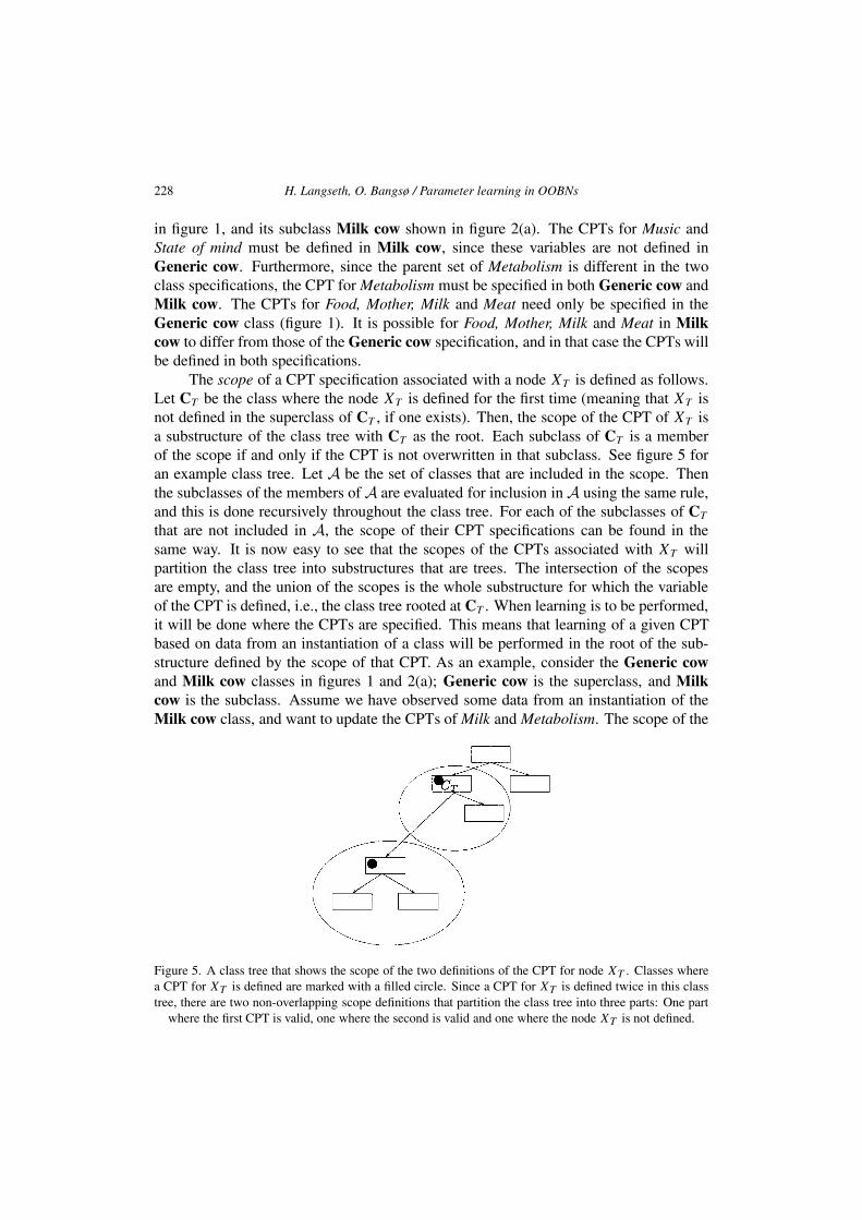
228 H. Langseth, O. Bangsø / Parameter learning in OOBNs
in figure 1, and its subclass Milk cow shown in figure 2(a). The CPTs for Music andState of mind must be defined in Milk cow, since these variables are not defined inGeneric cow. Furthermore, since the parent set of Metabolism is different in the twoclass specifications, the CPT for Metabolism must be specified in both Generic cow andMilk cow. The CPTs for Food, Mother, Milk and Meat need only be specified in theGeneric cow class (figure 1). It is possible for Food, Mother, Milk and Meat in Milkcow to differ from those of the Generic cow specification, and in that case the CPTs willbe defined in both specifications.
The scope of a CPT specification associated with a node XT is defined as follows.Let CT be the class where the node XT is defined for the first time (meaning that XT isnot defined in the superclass of CT , if one exists). Then, the scope of the CPT of XT isa substructure of the class tree with CT as the root. Each subclass of CT is a memberof the scope if and only if the CPT is not overwritten in that subclass. See figure 5 foran example class tree. Let A be the set of classes that are included in the scope. Thenthe subclasses of the members of A are evaluated for inclusion in A using the same rule,and this is done recursively throughout the class tree. For each of the subclasses of CT
that are not included in A, the scope of their CPT specifications can be found in thesame way. It is now easy to see that the scopes of the CPTs associated with XT willpartition the class tree into substructures that are trees. The intersection of the scopesare empty, and the union of the scopes is the whole substructure for which the variableof the CPT is defined, i.e., the class tree rooted at CT . When learning is to be performed,it will be done where the CPTs are specified. This means that learning of a given CPTbased on data from an instantiation of a class will be performed in the root of the sub-structure defined by the scope of that CPT. As an example, consider the Generic cowand Milk cow classes in figures 1 and 2(a); Generic cow is the superclass, and Milkcow is the subclass. Assume we have observed some data from an instantiation of theMilk cow class, and want to update the CPTs of Milk and Metabolism. The scope of the
Figure 5. A class tree that shows the scope of the two definitions of the CPT for node XT . Classes wherea CPT for XT is defined are marked with a filled circle. Since a CPT for XT is defined twice in this classtree, there are two non-overlapping scope definitions that partition the class tree into three parts: One part
where the first CPT is valid, one where the second is valid and one where the node XT is not defined.
H. Langseth, O. Bangsø / Parameter learning in OOBNs 229
Milk specification in the class tree is equal to the whole tree (we assume that Milk is notoverwritten in the subclass). Learning of the CPT for Milk will therefore be performedin the root of the class tree, i.e., in the Generic cow class. The CPT of Metabolismis overwritten in the Milk cow specification, so learning of Metabolism is performedin the Milk cow class. Note that no learning is performed in the instantiations; we donot update the CPTs of the underlying BN during learning. After a re-compilation ofthe OOBN, the CPTs from the class specifications are distributed to the instantiations asdescribed in [4], and at that point the underlying BN is updated as well.
One of the consequences of this is that another subclass of Generic cow, say Meatcow, might be updated because of the learning performed in Milk cow. In figure 2(b)the class specification for Meat cow is shown. This class has the same CPTs in Food,Mother, Milk and Meat as Generic cow (we assume they are not overwritten in Meatcow). Hence, the data from the instantiation of Milk cow used to update Milk will alsochange the instantiations of Meat cow. If this is not desirable, the CPTs of Generic cowshould be overwritten in the subclasses, e.g., the milk production of a milk cow could bedifferent from a generic cow, and the meat production could be different for meat cows.
In addition to maintaining the OO assumption, the proposed learning algorithmalso has another important effect. If at least one of the CPTs are shared by more thanone instantiation, the number of parameters to learn is reduced. This is desirable, asshown in the following.
2.1. The case of no missing data
When the database D is complete, i.e., we have no missing values, the learningtheory becomes particularly easy. To recapitulate, we have N independent realizationsfrom a distribution with distribution function f . Since the data is complete we canfind the maximum likelihood approximation fN by using closed-form equations insteadof applying the iterative EM algorithm. To test the learning algorithms we thereaftercalculate the KL divergence D(fN‖f ) between the estimated distribution fN and the
“true” distribution f . LetL→ denote convergence in distribution, meaning that if we have
an infinite sequence X1, X2, . . ., then we write XnL→X if and only if the distribution
functions Fn(x) of Xn converge to the distribution function F(x) of X for any continuitypoint x of F , where F(x) = ∑
x ′x f (x′) [27, definition 2.3.2]. Using large sample
theory it is easy (see [24] for details) to verify that when θ is an unbiased estimator of θ ,then
2N ·D(fN‖f
) L→|θ |∑i=1
(θi − θi
τi
)2
,
where τ 2i is the Cramér–Rao lower bound for the variance of an unbiased estimator for
θi , defined in [10, chapter 32]. Using this result, and the fact that we have complete data,

230 H. Langseth, O. Bangsø / Parameter learning in OOBNs
2N ·D(fN‖f ) converges towards a particular χ2 distribution:
2N ·D(fN‖f
) L→X ∼ χ2p, (2)
where p = |θ | is the size of the parameter space of f . Hence, as N grows large, we havean easily interpretable relationship for the expected value of the KL divergence
limN→∞ 2N · E[
D(fN‖f
)] = |θ |, (3)
which may be formulated as
E[D
(fN‖f
)] ≈ |θ |2N
(4)
for large N . Thus, not surprisingly, having fewer parameters will increase the expectedlearning speed as measured by the empirical KL divergence. Object-oriented learning re-duces the number of parameters to learn. Since learning is done in the class specification,we get fewer parameters to estimate (by constraining some of the existing parameters inthe underlying BN to be identical).
We define p, the effective number of parameters for the object-oriented learning,as the number of free parameters in the object oriented model. Hence, p is made up bythe sum of the free parameters in the CPTs of the class specifications instantiated in theOOBN. Remember that the complete OOBN is also an instantiation of a class (OMD’sStock-class). The number of parameters in the instantiations are not counted, as they areforced to be identical to the parameters in the class definitions.
To see that equation (2) is valid in object oriented learning with p = p, the keyproperty we need is that for a class with k instantiations, observing one case with all thek instantiations of the class has the same effect for learning the parameters in the objectoriented model as observing k hypothetical cases of the class. This follows triviallyfrom the asymptotic theory of statistics, as outlined below. Note that we suppress alltechnicalities from this discussion and without notice make use of the smoothness andstrict positivity of the distribution functions, and that all quantities involved are finitewith probability 1. The presentation below is based on [27], and in particular, chapter 7of that book.
In the current setting, it is well known that the Maximum Likelihood estimatesθN are asymptotically Gaussian distributed with mean θ and some variance , i.e.,
θNL→N (θ,). The Fisher Information matrix I is the |θ | × |θ | matrix defined by
Iij = −E
[∂2
∂θi∂θjlog f (X|θ)
].
The asymptotic variance of the maximum likelihood estimator θN can now be definedby the Fisher information, = (1/N)I−1 (given certain regularity conditions that arefulfilled in the setting of our work).
Let Y and Z be random variables distributed with density fθ (·) and gθ (·), respec-tively. Furthermore, let the information about θ from Y and Z be denoted IY and IZ ,

H. Langseth, O. Bangsø / Parameter learning in OOBNs 231
respectively. The information available by the sample Y ,Z, called I Y ,Z, is by us-ing [27, theorem 7.2.2] given as
I Y ,Z = IY + IZ (5)
when∂
∂θilog fθ (Y ) |= ∂
∂θjlog gθ (Z), i, j = 1, . . . , |θ |.
Since the maximum likelihood estimators are asymptotically efficient [27, sec-tion 7.6], and the empirical KL divergence is a function of θ through the parametervariances only, see [24], the information about θ in k instantiations equals the sum ofthe information in k imaginary cases of the class, as long as there are no missing data inthe database. The fact that equation (2) is valid in object-oriented learning with p = p
follows.To test the object oriented learning method, consider the example of OMD’s farm
as described in section 1.1. Assume OMD measures all the variables of the domainregularly, and stores them in a database. He wishes to estimate the parameters in hisdomain, and uses both the conventional as well as the object-oriented learning methods.The results are displayed in figure 6, where the asymptotic values of the expected KLdivergence of the two methods as a function of N according to equation (4) are indicatedas well. The conventional learning algorithm has 634 parameters to estimate, whereasthe object-oriented domain only has 322. Hence, according to equation (4) the KL diver-gence of the conventional learning algorithm is approximately 634/322 ≈ 1.97 times aslarge as the one of object-oriented learning for large N .
Figure 6. KL divergence between learned networks and the “true” distribution as a function of the size ofthe training set for the OMD network in figure 3 using complete data. The results from the OO learning aredrawn with solid line, whereas the conventional learning results are dotted. The large-sample approxima-
tions from equation (4) are drawn with thick lines.

232 H. Langseth, O. Bangsø / Parameter learning in OOBNs
2.2. Missing data
When learning with missing data, the relation in equation (3) no longer holds.Assume that the data is missing completely at random, and let q denote the probabilitythat a given variable Xi in a given data vector is missing. If q is “small” and the networkis sparsely connected, then it is argued in [24] that for conventional learning we have
limN→∞ 2N(1 − q) · E[
D(fN‖f
)] ≈ |θ |.Hence, the expected value of D(fN‖f ) is still approximately proportional to the num-ber of parameters asymptotically. This does not, however, guarantee that object orientedlearning is faster than conventional learning when some of the data is missing. To seethe problem, consider the simple example domain in figure 7. The underlying BN ofthe OOBN is shown, and two instantiations of a class are framed. We follow, e.g., [36]and include the unknown probability parameters θ in the model. The probability para-meters are drawn as filled circles, the empty circles are domain variables. Assume thatfor a given data record from the domain in figure 7 we have observed I1. X2 = x2 andX4 = x4. X4 is the common child of I1. X2 and I2. X2. However, I2. X2 is missing fromthe data sample. In this case we get into trouble when we want to learn the probabilityP(X2 = x2|X1 = x1), as the two pieces of information used in learning this prob-ability parameter are correlated (the observed value of I1. X2 influences both of them).Hence, the parameter estimates become dependent and thus the additivity of informationin equation (5) is no longer valid. However, since the information matrix I is positivesemi-definite [27, corollary 7.5.1], it follows that the information gain is always positive.Hence,
I Y ,Z IY , I Y ,Z IZ.
Figure 7. A simple example with two instantiations I1 and I2 of a class C. When doing object orientedlearning some of the parameters are constrained to be equal. This is indicated by dotted lines.

H. Langseth, O. Bangsø / Parameter learning in OOBNs 233
Using the fact that the maximum likelihood estimators are asymptotically efficient, wehave for large N
VarOO(θi
) VarConv
(θi
)for any parameter estimate θi where VarOO(·) denotes the parameter variance obtained byobject-oriented learning and VarConv(·) denotes the variance of the conventional learningestimates. The object-oriented learning will therefore not be worse than conventionallearning in expectation as measured by the empirical KL divergence. However, as q
grows large, the object-oriented learning may not be any better than the conventionalone either.
To test the object-oriented learning with missing data, we assume that OMD doesnot have the time to measure all the available information every day. Therefore, at thebeginning of the day he independently chooses to measure each variable with a proba-bility 1−q, or skip it that day (with probability q). This dataset is missing completely atrandom. The KL divergences that OMD achieves when learning both object oriented aswell as conventionally are depicted in figure 8 for different values of q. Object-orientedlearning is at least as good as the conventional one for all degrees of missing data, andfor all sample sizes. The results for q = 0.5 and q = 0.75 were obtained by random
Figure 8. KL divergence between learned networks and the true distribution as a function of the size of thetraining set. Object-oriented learning offers a KL divergence that in expectation is at least as small as the
one from conventional learning for all data sizes and all degrees of missing data.

234 H. Langseth, O. Bangsø / Parameter learning in OOBNs
restart of the EM algorithm up to 10 times, whereas the two other graphs were obtainedby only one run of the EM algorithm.
When some of the data is missing we can not guarantee the increased learningspeed that was obtained in the case of complete data. The method is, however, intu-itively more appealing, and one will not loose information by using the object-orientedapproach. The empirical results illustrated in figure 8 indicate that the object-orientedlearning is strictly better even with large amount of missing data.
3. Violating the OO assumption
The results in figures 6 and 8 show that the OOBN approach indeed works betterthan the conventional approach on our example network. This is hardly a surprise, sincewe know that all instantiations are identical, and object-oriented learning simply takesthis into account as part of its learning bias. More interesting is what happens if theinstantiations of a class are slightly different4 to each other. It may be reasonable toassume that the structure of all instantiations are identical, but that the parameters maybe somewhat different. In papers on parameter learning the authors typically state that:
“This [learning probability parameters in a BN with known structure and hidden vari-ables] is an important problem, because structure is much easier to elicit from expertsthan numbers.” [6, abstract]
A similar line of argument can be employed here: It is easy for an expert to say thatthe instantiations have identical structure. However, although the CPTs are about equal,there may be differences so small or subtle (e.g., due to variables not in the model thatdiffer between the individual instantiations) that they are difficult to quantify. In OMD’scase, for instance, no two cows are exactly alike, due to e.g., genetic differences.
We, therefore, propose a “relaxed OO” parameter learning, where differences be-tween instantiations of the same class are penalized, but not totally rejected. Note thatwhen applying “relaxed OO” learning the resulting network will not be object orientedany more. In this case the object orientation was merely a help during the networkdesign, and not necessarily an anticipated property of the network during routine use.
The framework we propose to use for this calculation is Bayesian Model Aver-aging (BMA), see, e.g., [20]. In BMA one has a set of competing statistical modelsM1,M2, . . . ,MK. To each model Mk a prior degree of belief, P(Mk), is attached.The posterior degree of belief (given the database D) can be calculated in the standardBayesian way,
P(Mk|D) = P(D|Mk) · P(Mk)∑K =1 P(D|M ) · P(M )
, (6)
4 If the instantiations are very different, a domain expert will not make the OO assumption. Proper modelingwould instead imply the use of subclasses to fulfill the OO assumption. We therefore expect this situationto occur when the domain is “almost” object oriented, but the theory outlined will also work when theinstantiations are very different, see the discussion leading to figure 10.
H. Langseth, O. Bangsø / Parameter learning in OOBNs 235
where
P(D|Mk) =∫
k
P (D|θk,Mk)P (θ k|Mk) dθ k. (7)
θ k is the model parameters given model Mk , and the integration is performed over thewhole parameter space k of θ k. If ! is the property of interest, the posterior distributionof ! according to BMA is
P(!|D) =K∑k=1
P(!|Mk,D)P (Mk|D). (8)
In our application ! will be the event that some variable takes on a particular value giventhe configuration of its parents, e.g., Xi = k | pa(Xi) = j. We use θO
ijk to denote theparameter estimate of θijk = P(Xi = k|pa(Xi) = j) in the object oriented learning, andθCijk in the case of conventional learning. The BMA estimate θB
ijk will be given by
θ Bijk = θ O
ijkP (MO |D)+ θ CijkP (MC |D). (9)
Here P(MO |D) and P(MC |D) are the posterior belief in the object oriented and con-ventional model, respectively. In [30] it is shown that when using a logarithmic scoringrule, averaging over all models provide better average predictive ability than using anysingle model Mj , conditioned on the set of models being considered.
The typical problem when implementing BMA is the computational complexity.First of all, the set of models can grow very large. Fortunately, this is not problematic inour case, as we limit the set of models to “Object oriented” and “Not object oriented”.Secondly, the integration in equation (7) may be difficult to perform. This is cumbersomealso in this work. As a first approximation one may crudely approximate the likelihoodby using a distribution for θ k that is degenerated at the maximum likelihood estimate.Using k = θ k in equation (6), our posterior belief would be approximated by
P(Mk|D) ≈ P(Mk|D, θ k = θ k
) = P(D|Mk, θ k) · P(Mk)∑K =1 P(D|M , θ ) · P(M )
. (10)
Note that equation (10) will over-estimate the likelihood of the data, especially forlarger models. Since the conventional model contains more parameters than the object-oriented one, we know that the likelihood of that model will be at least as large as thelikelihood of the object-oriented model. This tendency for choosing the more complexmodel leads to the well-known problem of over-fitting, and is due to the higher flexibilityof the more complex model. In our work we use an approximation to the log likelihoodwhere a model is penalized for its size. The approximation is known as the BayesianInformation Criteria (BIC):
log(P(D|Mk, θ k)
) ≈ log(P
(D|Mk, θ k
))− |θ k|2
log(N), (11)

236 H. Langseth, O. Bangsø / Parameter learning in OOBNs
where |θ k| is the number of free parameters for model Mk , and N is the size of the dataset. It is shown in [35] that the asymptotic size of the error in this approximation does notincrease with N . The BIC has earlier been applied for learning in Bayesian networks,see e.g., [17,18]. We now use equation (11) to modify the likelihood calculations inequation (10), and get
P(Mk|D) ≈ P(D|Mk, θ k) ·N−|θ k |/2 · P(Mk)∑K =1 P(D|M , θ ) ·N−|θ |/2 · P(M )
(12)
as our posterior belief in model Mk.The last problem of BMA is that of defining model priors. There is quite a lot of
work available on generating model priors in the framework of Bayesian networks, boththrough knowledge elicitation [29,30] and non-informed methods as in, e.g., [18]. Inour experience the domain experts find it difficult to assess priors for the two competingmodels at hand. Since the model he initially developed is object oriented he would liketo believe that the OO assumption is justified, and therefore tends to hold a large beliefin the object-oriented model. On the other hand, at a sufficiently detailed level the trulyobject-oriented real-world domains are very rare, and confronted by this fact the domainexpert tends to be in trouble when the belief is to be quantified. In the end, the domainexperts typically claim to be ignorant and give uniform priors, which is “. . . a reasonable‘neutral’ choice [when there is little prior information about the relative plausibility ofthe models considered].” [20, p. 390].
In the following we employ the BMA framework to a version of OMD’s domainthat is not object oriented: Without OMD’s knowledge, two of his cows have been givenhormones to produce more meat. Out of the two hormone-treated cows there is oneMeat cow and one Milk cow. The effect of the hormone treatment (in our model, wherefood quality is not an issue) is that the treated cows produce significantly more meat.Hence, the true probability distributions over the Meat node has been changed for bothcows. The rest of the domain is unchanged. The two Milk cows are thus not identicalanymore, as their probability tables match for all but the Meat node; the same goes forthe Meat cows. Since OMD does not know of this treatment, he models his stock inan object-oriented way, and wants to learn the probability tables in the domain from hisdata. He feels that his OO assumption is justified, and holds a prior belief of 75% for theobject-oriented model. The results are shown in figure 9.
As the domain is not entirely object oriented, but still has some similarity to anobject-oriented domain, the learning task of this example is a difficult one. The numberof parameters in the conventional BN learning is almost twice that of the object-orientedmodel. By equation (12) this will give OMD a high posterior belief in the object-orientedmodel even when the observed data is carrying strong evidence against the OO assump-tion (i.e., the node Meat differs in the different instantiations). OMD could have useda larger model space describing the intermediate cases more specifically, e.g., by con-sidering all models of the type “Nodes Xk, . . . , X are different between instantia-tions, but otherwise the domain is object oriented”. In this case the learning methodwould have discovered the violation of the OO assumption faster. The correct model
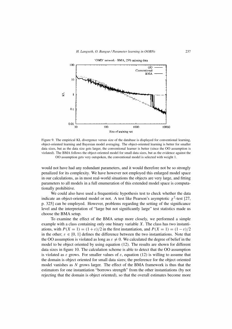
H. Langseth, O. Bangsø / Parameter learning in OOBNs 237
Figure 9. The empirical KL divergence versus size of the database is displayed for conventional learning,object-oriented learning and Bayesian model averaging. The object-oriented learning is better for smallerdata sizes, but as the data size gets larger, the conventional learner is better (since the OO assumption isviolated). The BMA follows the object-oriented model for small data sizes, but as the evidence against the
OO assumption gets very outspoken, the conventional model is selected with weight 1.
would not have had any redundant parameters, and it would therefore not be so stronglypenalized for its complexity. We have however not employed this enlarged model spacein our calculations, as in most real-world situations the objects are very large, and fittingparameters to all models in a full enumeration of this extended model space is computa-tionally prohibitive.
We could also have used a frequentistic hypothesis test to check whether the dataindicate an object-oriented model or not. A test like Pearson’s asymptotic χ2-test [27,p. 325] can be employed. However, problems regarding the setting of the significancelevel and the interpretation of “large but not significantly large” test statistics made uschoose the BMA setup.
To examine the effect of the BMA setup more closely, we performed a simpleexample with a class containing only one binary variable X. The class has two instanti-ations, with P(X = 1) = (1+ ε)/2 in the first instantiation, and P(X = 1) = (1− ε)/2in the other; ε ∈ [0, 1] defines the difference between the two instantiations. Note thatthe OO assumption is violated as long as ε = 0. We calculated the degree of belief in themodel to be object oriented by using equation (12). The results are shown for differentdata sizes in figure 10. The calculation scheme is able to detect that the OO assumptionis violated as ε grows. For smaller values of ε, equation (12) is willing to assume thatthe domain is object oriented for small data sizes; the preference for the object orientedmodel vanishes as N grows larger. The effect of the BMA framework is thus that theestimators for one instantiation “borrows strength” from the other instantiations (by notrejecting that the domain is object oriented), so that the overall estimates become more

238 H. Langseth, O. Bangsø / Parameter learning in OOBNs
Figure 10. Posterior belief in the preposition that the domain is object oriented calculated by equation (12)for different values of ε and different data sizes N .
robust. When more data is present, or when the observed data clearly indicate that theOO assumption is violated, this “borrowing” does not take place to the same extent.
The same kind of result can be obtained by building a hierarchical Bayesian model.In this setting, we model θijk in the different instantiations as random variables deter-mined by an underlying distribution %ijk . The posterior variance of %ijk determines howequal the instantiations of the classes are, see, e.g., [5] for a case-study.
4. Type uncertainty
So far we have assumed that the domain expert is able to unambiguously classifyeach instantiation of the domain to a specific class. However, this may not be realistic inreal-world applications. Not being able to classify an instantiation is an example of whatis called type uncertainty in [33]: The expert is uncertain about the type (or class in ourterminology) of an instantiation. As an example, assume OMD is unable to determinewhether COWl is a Milk cow or a Meat cow. Even though he is not able to determinethe class of COWl, he would like to learn from the available data. This section is devotedto showing how we treat type uncertainty within our framework.
Let the candidate classes of an instantiation I in an OOBN be given by the set SI.The expert encodes his prior beliefs about the class of the instantiation I as a distributionover SI. We assume that the probability distributions for the different instantiations areindependent a priori. Recall that we use the notation I.X to denote the variable X inthe instantiation I. ZI is the set of nodes that are defined inside the instantiation I (thatis, not including those input nodes of the instantiation that reference nodes outside I).Let I denote the set of all instantiations in the OOBN. We use T(I) to denote the classof an instantiation I, and T(I) to denote a classification of all the instantiations in thedomain. If we have a classification C = T(I), then C↓I is the induced classification ofa given instantiation I ∈ I . We use αI,C
for P(T(I) = C ). Furthermore, pa(I.X|T(I))

H. Langseth, O. Bangsø / Parameter learning in OOBNs 239
is used to denote the set of parents of I.X given the class of I. If Xi ∈ ZI, we use θ ,ijkfor the probability P(I.Xi = k|T(I) = C , pa(I.Xi|C ) = j). To avoid problems withoverfitting, we will assume that we have instantiations that are allocated to all classesin the OOBN model. If this is not the case, penalization of model complexity as inequation (11) should be introduced.
Let X denote the variables contained in the underlying BN. By means of the fun-damental factorization of a probability distribution encoded by a BN, and hence by anOOBN, we get:
P(X,T(I)
)=P(T(I)
) · P (X|T(I)
)=
∏I∈I
P(T(I)
) · [ ∏X ∈ZI
P(I.X |pa
(I.X |T(I)
), T(I)
)]. (13)
Note that for each choice of the classifications T(I) we have a different OOBN.The possible OOBNs are structurally identical everywhere except for the local modelsof the instantiations where the expert is uncertain. The correct OOBN is unknown, butwe hold a prior distribution over the possible candidates. A priori the different OOBNmodels are conditionally independent given the classification. The overall model cantherefore be modeled as an object oriented version of a Bayesian multinet; Bayesianmultinets were introduced in [15].
Our goal is to employ a learning algorithm that learns the parameters of a domain,without specifying the class of I more precisely than by a prior distribution over SI. Thiscan be done by standard use of the EM algorithm.5 In the following, we let α (t)
I,C denote
the estimate of P(T(I) = C ) after the t th iteration of the EM algorithm, and use α (t) to
denote the collection of these estimates at that time. Furthermore, (t) = θ (t)
,ijk is thecollection of probability parameter estimates in the classes after the t th iteration. Thealgorithm now proceeds by iterating over the following two update equations. First, wegenerate new estimates for αI,C
α(t)
I,C ←
∑C: C↓I=C
P (D|T(I) = C, (t−1)) · P(T(I) = C|α = α (t−1))∑
C P(D|T(I) = C, (t−1)) · P(T(I) = C|α = α (t−1))
. (14)
The sum in the denominator is taken over all possible classifications T(I), whereas thesum in the numerator is restricted to classifications where I is classified to class C .Note that P(T(I) = C|α = α (t−1)) is easy to calculate, since this probability is just theproduct of a subset of the elements in α(t−1).
Next, we update the estimates (t−1)
. Let I be the instantiation containing Xi , i.e.,Xi ∈ ZI. Then n
(I,C )ijk is the expected counts of the event Xi = k, pa(Xi|C ) = j
given that T(I) = C . The distribution over the possible classification of the other
5 To fit type uncertainty calculations into our OOBN framework, we will assume that for all C ∈ SI wehave that all nodes observed for I will be defined in ZI whenever T(I) = C . Technically this is notnecessary, but the implementation is simplified. Classes that do not meet this requirement cannot becandidate classes, and should therefore be removed.
Annals of Mathematics and Artificial Intelligence 32: 221–243, 2001. 2001 Kluwer Academic Publishers. Printed in the Netherlands.
Parameter learning in object-oriented Bayesian networks
Helge Langseth a,b and Olav Bangsø b
a Department of Mathematical Sciences, Norwegian University of Science and Technology, N-7491Trondheim, Norway
E-mail: [email protected] Department of Computer Science, Aalborg University, Fredrik Bajers Vej 7E,
DK-9220 Aalborg Øst, DenmarkE-mail: hl, [email protected]
This paper describes a method for parameter learning in Object-Oriented Bayesian Net-works (OOBNs). We propose a methodology for learning parameters in OOBNs, and provethat maintaining the object orientation imposed by the prior model will increase the learn-ing speed in object-oriented domains. We also propose a method to efficiently estimate theprobability parameters in domains that are not strictly object oriented. Finally, we attack typeuncertainty, a special case of model uncertainty typical to object-oriented domains.
Keywords: Bayesian networks, object orientation, learning
AMS subject classification: 68T05
1. Introduction
Bayesian Networks (BNs) [21,32] have established themselves as a powerful toolin many areas of artificial intelligence, including planning, vision, decision support sys-tems and robotics. However, one of the main obstacles is to create and maintain verylarge domain models. To remedy this problem, object-oriented versions of the BN frame-work have been proposed in the literature [4,22]. Object-Oriented BNs (OOBNs) as de-fined in these papers offer an easy way of creating BNs, but the problem of assessingand maintaining the probability estimates still remain; conventional learning algorithmslike [6] do not exploit that the domain is object oriented while learning.
In this paper we propose a learning method that is applied directly to the OOBNspecification. It is proven that this learning method is superior to conventional learningmethods in object oriented domains, and a method to efficiently estimate the probabilityparameters in domains that are not strictly object oriented is also proposed.
This paper is organized as follows: The rest of this section will create a startingpoint for our analysis by introducing OOBNs and the required notation and assump-tions. In section 2 we outline the proposed learning method, and in section 3 we pro-pose a framework for learning in domains that are only approximately object oriented.A special case of model uncertainty, typical to object-oriented domains, is handled insection 4, and we conclude in section 5.

240 H. Langseth, O. Bangsø / Parameter learning in OOBNs
instantiations, as well as conditional distributions over missing values, are replaced byexpected values in the E-step of the EM algorithm. Similarly, n(I,C )
ij =∑k n
(I,C )ijk is the
expected counts of the event pa(Xi|C ) = j under the assumption that T(I) = C .The estimates for θ(t)
,ijk in class C are updated by
θ(t) ,ijk ←
∑I∈I: Xi∈ZI
α(t−1)I,C · n(I,C )
ijk∑I∈I: Xi∈ZI
α(t−1)I,C · n(I,C )
ij
. (15)
Equation (15) is the natural extension of the update equation when the classification ofall instantiations are known. In that case, all values of α are fixed at either 0 or 1; theupdate rules are otherwise identical.
Iterating over the equations above will lead to a local maximum of the likelihood ofthe observed data. As a spin-off from the presented algorithm, equation (14) generatesthe posterior distribution over the possible classes of an instantiation. This task, whichis known as classification, has a rich body of literature also within the BN community,see, e.g., [7,13]. The complexity of performing the parameter update steps is exponentialin the number of instantiations the expert cannot classify with certainty. If the numberof these unclassified instantiations is “large”, it will be more efficient to implement aGeneralized EM algorithm, in which the likelihood of the data is strictly increased ineach iteration (but not necessarily maximized).
When we are only interested in classification (i.e., when the parameters are known),the type uncertainty task can be particularly easy computationally. First of all, we need
Figure 11. The empirical KL divergence versus the size of the database is displayed for object orientedlearning with correct classification of COW1 (Meat cow), wrong classification of COW1 (Milk cow), andthe results of the outlined method. The classification is fairly random for smaller data sizes, but as the datasize gets larger the correct class is given a probability converging towards 1. The results of the correct
classifier (thin line) are hidden underneath the results of the type uncertainty (thick line).

H. Langseth, O. Bangsø / Parameter learning in OOBNs 241
not perform the calculations in equation (15) since the parameters are known. Secondly,if the input and output sets of the classes in SI do not contain missing values, the requiredlikelihoods to classify I can be calculated locally (in the classes), and the larger modelin which the instantiation is embedded will be of no interest for the type uncertaintycalculations.
As an example, consider again OMD’s stock. Assume he is uncertain about theclass of COWl, whereas he is able to correctly classify the other three cows. His priordistribution for the class of COWl is that both classes are equally likely, and his datais reported with 25% missing values. In figure 11 the result of applying the proposedlearning algorithms (equations (14) and (15)) are displayed, together with the results ofa consistently wrong classifier (COWl assumed to be a Milk cow), an the consistentlycorrect classifier (COWl assumed to be a Meat cow). The proposed method is capableof detecting the correct class after approximately 700 cases, and for larger data sizes theresults of the proposed method are just as good as the consistently correct classifier.
5. Conclusions
In this paper we have proposed a learning method to learn parameters in OOBNs. Ithas been proven that this learning method is superior to conventional learning in object-oriented domains if the database is complete, and it is shown that as long as the OOassumption holds, the proposed learning algorithm will never be inferior to conventionallearning. We have proposed to use Bayesian model averaging to estimate the probabilityparameters in domains that are not strictly object oriented, and showed by example thatthis methodology offers reasonable results. A method that enables us to handle situationswhere the object oriented model is not completely specified has also been described.
Acknowledgements
We would like to thank our colleagues in the Decision Support Systems group atAalborg University for interesting discussions. In particular, Thomas D. Nielsen hasprovided constructive comments to an earlier version of this paper.
References
[1] N. Abe, M.K. Warmuth and J. Takeuchi, Polynomial learnability of probabilistic concepts with respectto the Kullback–Leibler divergence, in: Proceedings of the 4th Annual Workshop on ComputationalLearning Theory (COLT 1991) (Morgan Kaufmann, San Mateo, CA, 1991) pp. 277–289.
[2] O. Bangsø, H. Langseth and T.D. Nielsen, Structural learning in object oriented domains, in: Proceed-ings of the 14th International Florida Artificial Intelligence Research Society Conference (FLAIRS-2001) (AAAI Press, 2001) pp. 340–344.
[3] O. Bangsø and P.-H. Wuillemin, Object oriented Bayesian networks. A framework for topdown speci-fication of large Bayesian networks with repetitive structures, Technical Report CIT-87.2-00-obphw1,Department of Computer Science, Aalborg University (2000).
242 H. Langseth, O. Bangsø / Parameter learning in OOBNs
[4] O. Bangsø and P.-H. Wuillemin, Top-down construction and repetitive structures representation inBayesian networks, in: Proceedings of the 13th International Florida Artificial Intelligence ResearchSociety Conference, eds. J. Etheredge and B. Manaris (AAAI Press, 2000) pp. 282–286.
[5] R. Bellazzi and A. Riva, Learning conditional probabilities with longitudinal data, in: Working Notesof the IJCAI Workshop Building Probabilistic Networks: Where Do the Numbers Come from? (AAAIPress, Montreal, 1995) pp. 7–15.
[6] J. Binder, D. Koller, S. Russell and K. Kanazawa, Adaptive probabilistic networks with hidden vari-ables, Machine Learning 29 (1997) 213–244.
[7] J. Cheng and R. Greiner, Comparing Bayesian network classifiers, in: Proceedings of the 15th Con-ference on Uncertainty in Artificial Intelligence, UAI’99, eds. K.B. Laskey and H. Prade (MorganKaufmann, Stocholm, 1999) pp. 101–108.
[8] T.M. Cover and J.A. Thomas, Elements of Information Theory (Wiley, New York, 1991).[9] R.G. Cowell, A.P. Dawid, S.L. Lauritzen and D.J. Spiegelhalter, Probabilistic Networks and Expert
Systems, Statistics for Engineering and Information Sciences (Springer, New York, 1999).[10] H. Cramér, Mathematical Methods of Statistics (Princeton University Press, Princeton, NJ, 1946).[11] S. Dasgupta, The sample complexity of learning fixed-structure Bayesian networks, Machine Learn-
ing 29(2–3) (1997) 165–180.[12] A.P. Dempster, N.M. Laird and D.B. Rubin, Maximum likelihood from incomplete data via the EM
algorithm, Journal of the Royal Statistical Society, Series B 39 (1977) 1–38.[13] N. Friedman, D. Geiger and M. Goldszmidt, Bayesian network classifiers, Machine Learning 29
(1997) 131–163.[14] N. Friedman and Z. Yakhini, On the sample complexity of learning Bayesian networks, in: Pro-
ceedings of the 12th Annual Conference on Uncertainty in Artificial Intelligence (UAI-96) (MorganKaufmann, San Francisco, CA, 1996) pp. 274–282.
[15] D. Geiger and D. Heckerman, Knowledge representation and inference in similarity networks andBayesian multinets, Artificial Intelligence 82 (1996) 45–74.
[16] P.J. Green, On use of the EM algorithm for penalized likelihood estimation, Journal of the RoyalStatistical Society 52(3) (1990) 443–452.
[17] D. Heckerman, A tutorial on learning with Bayesian networks, in: Learning in Graphical Models, ed.M.I. Jordan (MIT Press, Cambridge, MA, 1999).
[18] D. Heckerman, D. Geiger and D.M. Chickering, Learning Bayesian networks: The combination ofknowledge and statistical data, Machine Learning 20 (1995) 197–243. Also available as MicrosoftResearch Technical Report MSR-TR-94-09.
[19] D.F. Heitjan and S. Basu, Distinguishing “Missing At Random” and “Missing Completely At Ran-dom”, The American Statistician 50(3) (1996) 207–213.
[20] J. Hoeting, D. Madigan, A. Raftery and C.T. Volinsky, Bayesian model averaging: A tutorial (with dis-cussion), Statistical Science 14(4) (1999) 382–417. Corrected version at http://www.stat.washington.edu/www/research/online/hoetingl999.pdf.
[21] F.V. Jensen, An Introduction to Bayesian Networks (Taylor and Francis, London, UK, 1996).[22] D. Koller and A. Pfeffer, Object-oriented Bayesian networks, in: Proceedings of the 13th Conference
on Uncertainty in Artificial Intelligence, eds. D. Geiger and P.P. Shenoy (Morgan Kaufmann, SanFrancisco, 1997) pp. 302–313.
[23] W. Lam and F. Bacchus, Learning Bayesian belief networks: An approach based on the MDL princi-ple, Computational Intelligence 10(4) (1994) 269–293.
[24] H. Langseth, Efficient parameter learning: Empiric comparison of large sample behaviour, Depart-ment of Computer Science, Aalborg University (2000). Available at http://www.cs.auc.dk/research/DSS/publications.
[25] K.B. Laskey and S.M. Mahoney, Network fragments: Representing knowledge for constructing prob-abilistic models, in: Proceedings of the 13th Conference on Uncertainty in Artificial Intelligence, eds.D. Geiger and P. Shenoy, (Morgan Kaufmann Publishers, San Francisco, CA, 1997) pp. 334–341.
H. Langseth, O. Bangsø / Parameter learning in OOBNs 243
[26] S.L. Lauritzen, The EM-algorithm for graphical association models with missing data, ComputationalStatistics and Data Analysis 19 (1995) 191–201.
[27] E.L. Lehmann, Elements of Large-Sample Theory, Springer Texts in Statistics (Springer, New York,1999).
[28] R.J.A. Little and D.B. Rubin, Statistical Analysis with Missing Data (Wiley, New York, 1987).[29] D. Madigan, J. Gavrin and A. Raftery, Eliciting prior information to enhance the predictive perfor-
mance of Bayesian graphical models, Communication in Statistics – Theory and Methods 24 (1995)2271–2292.
[30] D. Madigan and A. Raftery, Model selection and accounting for model uncertainty in grahical modelsusing Occam’s window, Journal of American Statistical Association 89 (1994) 1535–1546.
[31] L. Ortiz and L. Kaelbling, Accelerating EM: An empirical study, in: Proceedings of the 15th AnnualConference on Uncertainty in Artificial Intelligence (UAI-99) (Morgan Kaufmann, San Francisco,CA, 1999) pp. 512–521.
[32] J. Pearl, Probabilistic Reasoning in Intelligent Systems: Networks of Plausible Inference (MorganKaufmann, San Mateo, CA, 1988).
[33] A.J. Pfeffer, Probabilistic reasoning for complex systems, Ph.D. thesis, Stanford University (2000).[34] M. Pradhan, G. Provan, B. Middleton and M. Henrion, Knowledge engineering for large belief net-
works, in: Proceedings of the 10th Conference on Uncertainty in Artificial Intelligence (Morgan Kauf-mann, San Francisco, CA, 1994) pp. 484–490.
[35] G. Schwarz, Estimating the dimension of a model, Annals of Statistics 6 (1978) 461–464.[36] D.J. Spiegelhalter and S.L. Lauritzen, Sequential updating of conditional probabilities on directed
graphical structures, Networks 20 (1990) 579–605.[37] S. Srinivas, A probabilistic approach to hierarchical model-based diagnosis, in: Proceedings of the
10th Conference on Uncertainty in Artificial Intelligence (Morgan Kaufmann, San Francisco, CA,1994) pp. 538–545.
[38] B. Thiesson, Accelerating quantification of Bayesian networks with incomplete data, in: Proceedingsof the 1st International Conference on Knowledge Discovery and Data Mining (AAAI Press, MenloPark, CA, 1995) pp. 306–311.
[39] R.A. van Engelen, Approximating Bayesian belief networks by arc removal, IEEE Transactions onPattern Analysis and Machine Intelligence 19(8) (1997) 916–920.
[40] J. Whittaker, Graphical Models in Applied Multivariate Statistics (Wiley, Chichester, 1990).[41] Y. Xiang and F.V. Jensen, Inference in multiply sectioned Bayesian networks with extended Shafer-
Shenoy and lazy propagation, in: Proceedings of the 15th Conference on Uncertainty in ArtificialIntelligence, UAI’99, eds. K.B. Laskey and H. Prade (Morgan Kaufmann, Stocholm, 1999) pp. 680–687.
[42] Y. Xiang, D. Poole and M.P. Beddoes, Multiply sectioned Bayesian networks and junction forests forlarge knowledge-based systems, Computational Intelligence 9(2) (1993) 171–220.

V
Fusion of Domain Knowledge with Data for Structural Learning in
Object Oriented Domains


To appear in Journal of Machine Learning Research
Fusion of Domain Knowledge with Data for StructuralLearning in Object Oriented Domains
Helge Langseth∗[email protected]
Thomas D. Nielsen [email protected]
Department of Computer Science, Aalborg UniversityFredrik Bajers Vej 7E, DK-9220 Aalborg Ø, Denmark
Editor: Richard Dybowski
Abstract
When constructing a Bayesian network, it can be advantageous to employ structural learn-ing algorithms to combine knowledge captured in databases with prior information providedby domain experts. Unfortunately, conventional learning algorithms do not easily incor-porate prior information, if this information is too vague to be encoded as properties thatare local to families of variables. For instance, conventional algorithms do not exploit priorinformation about repetitive structures, which are often found in object oriented domainssuch as computer networks, large pedigrees and genetic analysis.
In this paper we propose a method for doing structural learning in object orienteddomains. It is demonstrated that this method is more efficient than conventional algo-rithms in such domains, and it is argued that the method supports a natural approach forexpressing and incorporating prior information provided by domain experts.Keywords: Bayesian networks, structural learning, object orientation, knowledge fusion
1. Introduction
The Bayesian network (BN) framework (Pearl, 1988, Jensen, 1996, 2001) has establisheditself as a powerful tool in many areas of artificial intelligence. However, eliciting a BNfrom a domain expert can be a laborious and time consuming process. Thus, methods forlearning the structure of a BN from data have received much attention during the last years,for an overview see e.g. (Buntine, 1996, Krause, 1998). Current learning methods have beensuccessfully applied in learning the structure of BNs based on databases. Unfortunately,though, only to a small extent do these methods incorporate prior information providedby domain experts. Prior information is typically encoded by specifying a prior BN hence,this information is restricted to the occurrence/absence of edges between specific pairs ofvariables.
In domains that can appropriately be described using an object oriented language (Ma-honey and Laskey, 1996, Mathiasen et al., 2000) we typically find e.g. repetitive substruc-tures or substructures that can naturally be ordered in a superclass–subclass hierarchy. Forsuch domains, the expert is usually able to provide information about these properties.
∗. Current address: Department of Mathematical Sciences, Norwegian University of Science and Technol-ogy, N-7491 Trondheim, Norway. [email protected].
c©2002 Helge Langseth and Thomas D. Nielsen.
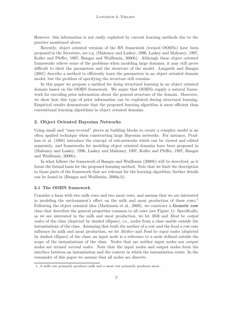
Langseth & Nielsen
However, this information is not easily exploited by current learning methods due to thepractice mentioned above.
Recently, object oriented versions of the BN framework (termed OOBNs) have beenproposed in the literature, see e.g. (Mahoney and Laskey, 1996, Laskey and Mahoney, 1997,Koller and Pfeffer, 1997, Bangsø and Wuillemin, 2000b). Although these object orientedframeworks relieve some of the problems when modeling large domains, it may still provedifficult to elicit the parameters and the structure of the model. Langseth and Bangsø(2001) describe a method to efficiently learn the parameters in an object oriented domainmodel, but the problem of specifying the structure still remains.
In this paper we propose a method for doing structural learning in an object orienteddomain based on the OOBN framework. We argue that OOBNs supply a natural frame-work for encoding prior information about the general structure of the domain. Moreover,we show how this type of prior information can be exploited during structural learning.Empirical results demonstrate that the proposed learning algorithm is more efficient thanconventional learning algorithms in object oriented domains.
2. Object Oriented Bayesian Networks
Using small and “easy-to-read” pieces as building blocks to create a complex model is anoften applied technique when constructing large Bayesian networks. For instance, Prad-han et al. (1994) introduce the concept of sub-networks which can be viewed and editedseparately, and frameworks for modeling object oriented domains have been proposed in(Mahoney and Laskey, 1996, Laskey and Mahoney, 1997, Koller and Pfeffer, 1997, Bangsøand Wuillemin, 2000b).
In what follows the framework of Bangsø and Wuillemin (2000b) will be described, as itforms the formal basis for the proposed learning method. Note that we limit the descriptionto those parts of the framework that are relevant for the learning algorithm; further detailscan be found in (Bangsø and Wuillemin, 2000a,b).
2.1 The OOBN framework
Consider a farm with two milk cows and two meat cows, and assume that we are interestedin modeling the environment’s effect on the milk and meat production of these cows.1
Following the object oriented idea (Mathiasen et al., 2000), we construct a Generic cowclass that describes the general properties common to all cows (see Figure 1): Specifically,as we are interested in the milk and meat production, we let Milk and Meat be outputnodes of the class (depicted by shaded ellipses), i.e., nodes from a class usable outside theinstantiations of the class. Assuming that both the mother of a cow and the food a cow eatsinfluence its milk and meat production, we let Mother and Food be input nodes (depictedby dashed ellipses) of the class; an input node is a reference to a node defined outside thescope of the instantiations of the class. Nodes that are neither input nodes nor outputnodes are termed normal nodes. Note that the input nodes and output nodes form theinterface between an instantiation and the context in which the instantiation exists. In theremainder of this paper we assume that all nodes are discrete.
1. A milk cow primarily produces milk and a meat cow primarily produces meat.
2

Knowledge Fusion for Structural Learning in OO Domains
A class may be instantiated several times with different nodes having influence on thedifferent instantiations through the input nodes hence, only the state space (the statesand their ordering) of the input nodes is known at the time of specification2 (e.g. thecows might have different mothers). To avoid ambiguity when referring to a node in aspecific instantiation, the name of the node will sometimes be prefixed by the name of theinstantiation (i.e., Instantiation-name.Node-name).
Food
bolismMeta-
Mother
Milk Meat
Generic cow
Figure 1: General properties common to all cows are described using the class Genericcow. The arrows are links as in normal BNs. The dashed ellipses are inputnodes, and the shaded ellipses are output nodes.
In order to model the different properties of milk cows and meat cows, we introducethe two classes Milk cow and Meat cow (see Figure 2). These two cow specificationsare subclasses of the Generic cow class (hence the “IS A Generic cow” in the top leftcorner of each of the class specifications). In a general setting, a class S can be a subclassof another class C if S contains at least the same set of nodes as C. This ensures thatan instantiation of S can be used anywhere in the OOBN instead of an instantiation ofC (e.g., an instantiation of Milk cow can be used instead of an instantiation of Genericcow). Each node in a subclass inherits the conditional probability table (CPT) of thecorresponding node in its superclass unless the parent sets differ, or the modeler explicitlyoverwrites the CPT. The sub–superclass relation is transitive but not anti-symmetric, soto avoid cycles in the class hierarchy it is required that a subclass of a class cannot be asuperclass of that class as well. Furthermore, multiple inheritance is not allowed, so thestructure of the class hierarchy will be a tree or a collection of disjoint trees (called a forest).
Finally, to model the four cows in the live-stock we construct a class Stock that encap-sulates the corresponding instantiations. In Figure 3 the boxes represent instantiations, e.g.Cow1 is an instantiation of the class Meat cow, which is indicated by Cow1:Meat cowinside the Cow1 instantiation. Note that only input nodes and output nodes are visible,as they are the only part of an instantiation which directly interact with the encapsulat-ing context (in this case the Stock class); this does not impose any constraints on whichvariables may be observed, it is merely a design technique to easier maintain large domainmodels. The double arrows are reference links. A reference link indicates that the leaf of
2. This is also referred to as strong type-checking, see (Bangsø and Wuillemin, 2000a) for details.
3

Langseth & Nielsen
Food
Meta-
mind
Music
bolismState of
Mother
Milk cow IS A Generic cow
MeatMilk
Mother
mind
State of
Weather
Meta-bolism
Food
Meat cow IS A Generic cow
MeatMilk
a) The Milk cow specification b) The Meat cow specification
Figure 2: a) A refined specification of a Milk cow. b) A refined specification of a Meatcow.
the link is a reference (or pointer) to the root of that link.3 For instance, the input nodeMother of Cow1 is a reference to the node Daisy. This means that whenever the nodeMother is used inside the instantiation Cow1, the node Daisy will be the node actuallyused (e.g., during inference).
MathildaWeatherFood
Cow1:Meat cow
Food WeatherMother
Cow3:Milk cow
FoodMother Mother
Cow4:Milk cow
MusicFood MotherFood Weather Music
MusicDaisy
Stock
Cow2:Meat cow
MeatMilk Milk Meat Milk Meat Milk Meat
Figure 3: The Stock class with two instantiations of the Milk cow class and two instan-tiations of the Meat cow class. Note that some input nodes are not referencingany nodes.
If there is more than one instantiation of a class (e.g. Cow1 and Cow2), the OOBNframework gives rise to the OO assumption (Langseth and Bangsø, 2001). This assumptionstates that the CPTs of one instantiation of a class are identical to the correspondingCPTs of any other instantiation of that class (meaning that the domains of the CPTs arecompatible and that the table entries are identical).
As the subclasses in a class hierarchy may have a larger set of nodes than their super-classes, the input set of a subclass S might be larger than the input set of its superclassC. Thus, if an instantiation of S is used instead of an instantiation of C, the extra input
3. To avoid confusion with the normal links in the model we do not use the terms “parent” and “child”when referring to reference links.
4

Knowledge Fusion for Structural Learning in OO Domains
nodes will not be referencing any nodes. To ensure that these nodes are associated withpotentials, the notion of a default potential is introduced: A default potential is a probabil-ity distribution over the states of an input node, which is used when the input node is notreferencing any node. Note that a default potential can also be used when no reference linkis specified, even if this is not a consequence of subclassing. As an example we have thatnot all the Mother nodes in Figure 3 reference a node, but because of the default potentialall nodes are still associated with a CPT. It is also worth noticing that the structure ofreferences is always a tree or a forest; cycles of reference links are not possible (Bangsø andWuillemin, 2000a).
Finally, inference can be performed by translating the OOBN into a multiply-sectionedBayesian network (Xiang et al., 1993, Xiang and Jensen, 1999), see (Bangsø and Wuil-lemin, 2000a) for details on this translation. Alternatively, we can construct the underlyingBN of the OOBN: The underlying BN of an instantiation I, BNI, is the (conventional)BN that corresponds to I including all encapsulated instantiations. There is exactly onesuch underlying BN for a given instantiation, and it can be constructed using the followingalgorithm (Langseth and Bangsø, 2001):
Algorithm 1 (Underlying BN)
1. Let BNI be the empty graph.
2. Add a node to BNI for all input nodes, output nodes and normal nodes in I.
3. Add a node to BNI for each input node, output node and normal node of the in-stantiations encapsulated in I, and prefix the name of the instantiation to the nodename (Instantiation-name.Node-name). Do the same for instantiations containedin these instantiations, and so on.
4. Add a link for each normal link in I, and repeat this for all instantiations as above.
5. For each reference tree, merge all the nodes into one node. This node is given all theparents and children (according to the normal links) of the nodes in the reference treeas its family. Note that only the root of the tree can have parents, as all other nodesare references to this node.
An input node that does not reference another node will become a normal node equippedwith a default potential; this can also be seen in Figure 4 which depicts the underlying BNof an instantiation of the Stock-class (Figure 3).
Cow4.
mindState of
Cow1. Cow2. Cow3. Cow4.
MotherCow4.Cow2.
Meat MilkMilkMilkMilkCow1. Cow1.
MeatCow2. Cow3.Cow2. Cow3.
Meat
MotherWeather
State of
FoodDaisy Mathilda Music
Cow4. Cow4.Meat
Metabolism
Cow1.
mindMetabolism Metabolism MetabolismState of
Cow2.
mindState of
Cow3.
mind
Figure 4: The underlying BN for the OOBN depicted in Figure 3.
5
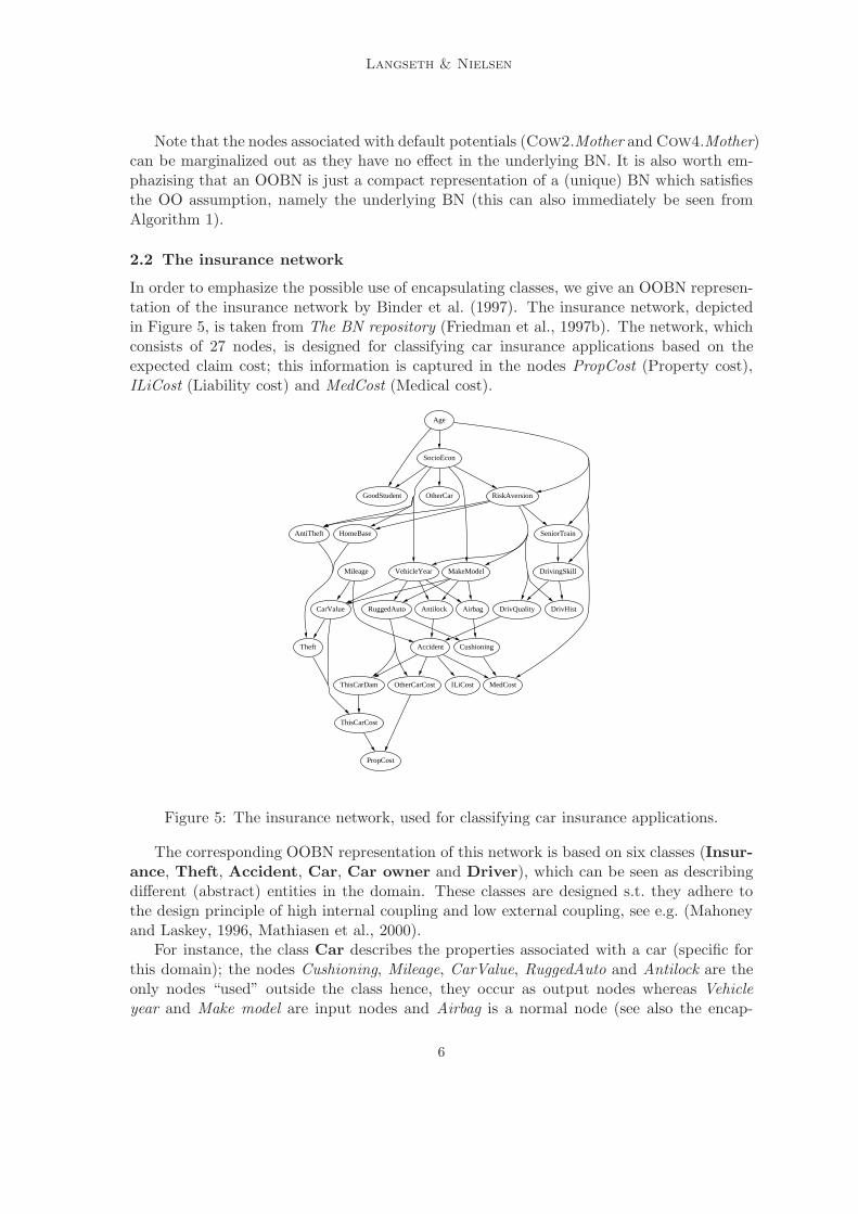
Langseth & Nielsen
Note that the nodes associated with default potentials (Cow2.Mother and Cow4.Mother)can be marginalized out as they have no effect in the underlying BN. It is also worth em-phazising that an OOBN is just a compact representation of a (unique) BN which satisfiesthe OO assumption, namely the underlying BN (this can also immediately be seen fromAlgorithm 1).
2.2 The insurance network
In order to emphasize the possible use of encapsulating classes, we give an OOBN represen-tation of the insurance network by Binder et al. (1997). The insurance network, depictedin Figure 5, is taken from The BN repository (Friedman et al., 1997b). The network, whichconsists of 27 nodes, is designed for classifying car insurance applications based on theexpected claim cost; this information is captured in the nodes PropCost (Property cost),ILiCost (Liability cost) and MedCost (Medical cost).
SocioEcon
GoodStudent RiskAversion
VehicleYear MakeModel
AntiTheft HomeBase
OtherCar
Age
DrivingSkill
SeniorTrain
MedCost
DrivQuality DrivHistRuggedAuto AntilockCarValue Airbag
Accident
ThisCarDam OtherCarCost ILiCost
ThisCarCost
Cushioning
Mileage
PropCost
Theft
Figure 5: The insurance network, used for classifying car insurance applications.
The corresponding OOBN representation of this network is based on six classes (Insur-ance, Theft, Accident, Car, Car owner and Driver), which can be seen as describingdifferent (abstract) entities in the domain. These classes are designed s.t. they adhere tothe design principle of high internal coupling and low external coupling, see e.g. (Mahoneyand Laskey, 1996, Mathiasen et al., 2000).
For instance, the class Car describes the properties associated with a car (specific forthis domain); the nodes Cushioning, Mileage, CarValue, RuggedAuto and Antilock are theonly nodes “used” outside the class hence, they occur as output nodes whereas Vehicleyear and Make model are input nodes and Airbag is a normal node (see also the encap-
6

Knowledge Fusion for Structural Learning in OO Domains
sulated instantiation C:Car in Figure 6). As another example, consider the class Driverwhich models the driving characteristics of a car owner. In the insurance context, drivingcharacteristics are an integral part of the notion of a car owner and (by the above men-tioned design principle) an instantiation of Driver is therefore encapsulated in the classCarOwner. The class Insurance encapsulates the corresponding instantiations of theother classes. Figure 6 depicts the final OOBN model (i.e., the Insurance class). Notethat only the interfaces of the encapsulated instantiations are shown.
ThisCarDam
CarCostOther-
D:Driver
Insurance
C:CarT:Theft
CO:CarOwner
SocioEcon SocioEcon Age
HomeBase
AntiTheft
DrivQuality
DrivQuality
MakeModelVehicleYear
RiskAversion
Mileage
A:Accident
AccidentCarValue
MileageCushioning
DrivQuality
AntilockAntilock
VehicleYear MakeModel
AgeAge
HomeBase
AntiTheft
CarValueTheft
MedCost PropCostThisCarCost
RuggedAuto
ILiCost
Figure 6: An OOBN representation of the insurance network. Notice that only the in-terfaces of the encapsulated instantiations are shown. Note also that we use aslightly non-standard graphical presentation for visualization purposes.
The Insurance-class is constructed s.t. the underlying BN of an instantiation of thatclass corresponds to the BN given in Figure 5. In this respect it is worth noticing theactive use of reference links: For example, there are two CarValue-nodes in the OOBN;C.CarValue is defined in C:Car, but as C.CarValue is a parent of T.Theft (confer alsothe underlying BN in Figure 5), it is imported into T:Theft using an input node (whichis named T.CarValue). The reference link between these two nodes shows that it is thesame random variable that is used in both situations. That is, T.CarValue is a reference toC.CarValue; this is required since CarValue is defined outside the scope of the instantiationsof the Theft-class.
2.3 OOBNs and dynamic Bayesian networks
An important set of Bayesian networks is dynamic Bayesian networks (DBNs), which modelthe stochastic evolution of a set of random variables over time, see e.g. (Kjærulff, 1992).
7

Langseth & Nielsen
Traditionally, a DBN specification consists of i) a BN over the variables at t = 0, and ii) atransition BN over the variables at t = 0 and t = 1. These two networks can alternativelybe described using OOBN classes, where the time-dependence is encoded by self-referencesbetween nodes; a self-reference is a reference between a node and an input node in thesame class.4 More precisely, when using the OOBN framework for modeling DBNs weconstruct two classes: One class representing the time-slice at t = 0, and another class whoseinstantiations correspond to the time-slices at t > 0. The dependence relation between atime-slice and the previous time-slice is then represented using self-references within theclass specification, see also (Bangsø and Wuillemin, 2000b). Note that using OOBN classesfor modeling time-slices also supports the introduction of encapsulated instantiations withinthe time slices.
3. Structural learning
In what follows we review the basis for performing structural learning. The notation will,whenever possible, follow that of Cooper and Herskovits (1991) and Heckerman et al. (1995).
Consider a Bayesian network BN = (BS ,ΘBS) over a set of discrete variables X1,X2,
. . . ,Xn, where BS is the graphical structure and ΘBSis the quantitative information. To
describe BS, the qualitative aspects of BN , we will use the following notation: ri is thenumber of states for variable Xi, qi is the number of configurations over the parents for Xi
in BS (denoted by Πi), i.e., qi =∏
Xl∈Πirl, and Πi = j denotes the event that Πi takes on
its j’th configuration. For the quantitative properties, we use θijk = P (Xi = k|Πi = j, ξ)(we assume θijk > 0), where ξ is the prior knowledge. For ease of exposition we define:
Θij = ∪rik=1θijk; Θi = ∪qi
j=1Θij ; ΘBS= ∪n
i=1Θi .
Note that ∀i, j :∑ri
k=1 θijk = 1. Finally, we let D = D1, . . . ,DN denote a database of Ncases, where each case is a configuration x over the variables X = (X1, . . . ,Xn).
The task is now to find a structure BS that best describes the observed data, or in a moreabstract formulation, to find the parameter space ΩBS
which best restricts the parametersused to describe the family of probability distributions FΩBS
= f(x |Θ) : Θ ∈ ΩBS. For
example, let Ω′ be the parameter space required to describe all probability distributionscompatible with the complete graph for two binary variables X1 and X2 (see Figure 7a).With the above notation, Ω′ is defined s.t. (θ1, θ21, θ22) ∈ Ω′. For the empty graph in Figure7b, the parameter space Ω′′ ⊂ Ω′ corresponds to the parameter space Ω′ where θ21 = θ22,i.e., Ω′′ is a hyperplane in Ω′. Learning the structure BS is therefore equivalent to findingthe parameter space ΩBS
that best describes the data; when learning the structure of a BNthere is an injective mapping from the BN structure, BS , to the associated parameter spaceΩBS
. However, as we shall see in Section 5, when we focus on learning OOBNs this is nolonger true; some aspects of an OOBN (i.e., the OO-assumption) are not reflected in theunderlying graphical structure, and in that case it may be beneficial to think of structurallearning as learning a parameter space Ω.
4. Self-references differ from reference links as the root of a self-reference is defined inside the instantiation,whereas the root of a reference link is defined outside the scope of the instantiation.
8

Knowledge Fusion for Structural Learning in OO Domains
X1 X2 X1 X2
a) Complete graph b) Empty graph
Figure 7: The two BN model structures for the domain X = (X1,X2).
3.1 The BD metric
A Bayesian approach for measuring the quality of a BN structure BS , is its posteriorprobability given the database:
P (BS |D, ξ) = c · P (BS |ξ)P (D|BS , ξ),
where c = 1/(∑
B P (B|ξ)P (D|B, ξ)). The normalization constant c does not depend onBS , thus P (D, BS |ξ) = P (BS |ξ)P (D|BS , ξ) is usually used as the network score. Note thatthe main computational problem is the calculation of the marginal likelihood:
P (D|BS , ξ) =∫
ΘBS
P (D|BS ,ΘBS, ξ)P (ΘBS
|BS , ξ)dΘBS, (1)
since the integral is over all possible parameters (conditional probabilities) ΘBS, i.e., over
all possible BNs that encode at least the same conditional independence relations as thestructure BS .
Cooper and Herskovits (1991) showed that this probability can be computed in closedform based on the following five assumptions: 1) the database D is a multinomial samplefrom some Bayesian network BG with parameters ΘBG
, 2) the cases in the database Dare independent given the BN model, 3) the database is complete, i.e., there does notexist a case in D with missing values, 4) for any two configurations over the parents fora variable Xi, the parameters for the conditional probability distributions associated withXi are marginally independent, i.e., Θij ⊥⊥ Θij′ for j 6= j′, and 5) the prior distribution ofthe parameters in every Bayesian network BS has a Dirichlet distribution5, i.e., there existnumbers (virtual counts) N ′
ijk > 0 s.t.:
P (Θij |BS , ξ) =Γ(
∑rik=1 N ′
ijk)∏rik=1 Γ(N ′
ijk)
ri∏k=1
θN ′
ijk−1
ijk , (2)
where Γ is the Gamma function satisfying Γ(x + 1) = xΓ(x). Note that the virtual countscan be seen as pseudo counts similar to the sufficient statistics derived from the database.An implicit assumption by Cooper and Herskovits (1991) is parameter modularity: Thedensities of the parameters Θij depend only on the structure of the BN that is local tovariable Xi.
Now, let Nijk be the sufficient statistics, i.e., Nijk =∑N
l=1 γ(Xi = k,Πi = j : Dl), whereγ(Xi = k,Πi = j : Dl) takes on the value 1 if (Xi = k,Πi = j) occurs in case Dl, and 0
5. Cooper and Herskovits (1991) actually assumes a uniform distribution which is a special case of theDirichlet distribution; the correctness of this generalization is proven in (Cooper and Herskovits, 1992).
9

Langseth & Nielsen
otherwise. From assumption 1, 2 and 3 we then have:
P (D|BS ,ΘBS, ξ) =
n∏i=1
qi∏j=1
ri∏k=1
θNijk
ijk . (3)
Substituting Equation 3 into Equation 1 gives:
P (D|BS , ξ) =∫
ΘBS
n∏i=1
qi∏j=1
ri∏k=1
θNijk
ijk P (ΘBS|BS , ξ)dΘBS
, (4)
and by assumptions 4 and 5 we get:
P (D|BS , ξ) =n∏
i=1
qi∏j=1
∫Θij
ri∏k=1
θNijk
ijk
[Γ(
∑rik=1 N ′
ijk)∏rik=1 Γ(N ′
ijk)
ri∏k=1
θN ′
ijk−1
ijk
]dΘij
=n∏
i=1
qi∏j=1
Γ(∑ri
k=1 N ′ijk)∏ri
k=1 Γ(N ′ijk)
∫Θij
ri∏k=1
θNijk+N ′
ijk−1
ijk dΘij .
The expression∏ri
k=1 θNijk+N ′
ijk−1
ijk corresponds to the last term of the Dirichlet distributionfor the parameters Θij having counts Nijk + N ′
ijk. Since this is a probability distributionover the parameters, the value of the integral can be read directly from Equation 2 (theintegral over all parameters evaluates to 1) and we get:
P (D, BS |ξ) = P (BS |ξ)n∏
i=1
qi∏j=1
Γ(N ′ij)
Γ(Nij + N ′ij)
ri∏k=1
Γ(Nijk + N ′ijk)
Γ(N ′ijk)
, (5)
where Nij =∑ri
k=1 Nijk and N ′ij =
∑rik=1 N ′
ijk. This metric is known as the BD metric(Bayesian metric with Dirichlet priors), and it was first derived by Cooper and Herskovits(1992). Unfortunately it requires the specification of the virtual counts N ′
ijk for all variable–parent configurations and for all values i, j and k.
3.2 The BDe metric
One drawback of the BD metric is that networks, which are likelihood equivalent, neednot be given the same score.6 Note that data cannot be used to discriminate betweensuch networks. Another shortcoming of the BD metric is that it does not provide aneasy way of specifying prior information concerning network structure and parameters. Toovercome these problems, Heckerman et al. (1995) describe the BDe metric (Bayesian metricwith Dirichlet priors and equivalence) which gives the same score to likelihood equivalentnetworks. Hence, the metric is based on the concept of sets of likelihood equivalent networkstructures, where all members in a set are given the same score.
The BDe metric also provides a simple way of identifying the virtual counts N ′ijk (in
Equation 5) by having the user specify a prior Bayesian network Bp for X and an equivalentsample size N ′:
N ′ijk = P (Xi = k,Πi = j|Bp, ξ) ·N ′. (6)
6. Two networks are said to be likelihood equivalent if they encode the same assertions about conditionalindependence.
10
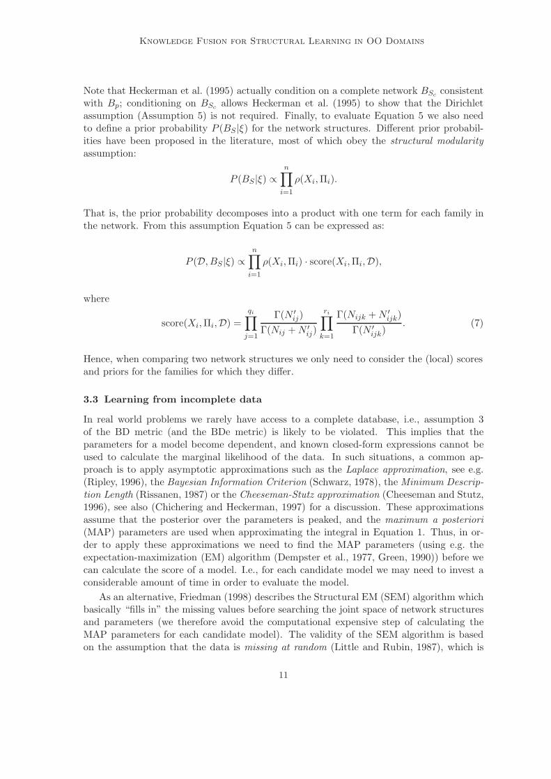
Knowledge Fusion for Structural Learning in OO Domains
Note that Heckerman et al. (1995) actually condition on a complete network BSc consistentwith Bp; conditioning on BSc allows Heckerman et al. (1995) to show that the Dirichletassumption (Assumption 5) is not required. Finally, to evaluate Equation 5 we also needto define a prior probability P (BS |ξ) for the network structures. Different prior probabil-ities have been proposed in the literature, most of which obey the structural modularityassumption:
P (BS |ξ) ∝n∏
i=1
ρ(Xi,Πi).
That is, the prior probability decomposes into a product with one term for each family inthe network. From this assumption Equation 5 can be expressed as:
P (D, BS |ξ) ∝n∏
i=1
ρ(Xi,Πi) · score(Xi,Πi,D),
where
score(Xi,Πi,D) =qi∏
j=1
Γ(N ′ij)
Γ(Nij + N ′ij)
ri∏k=1
Γ(Nijk + N ′ijk)
Γ(N ′ijk)
. (7)
Hence, when comparing two network structures we only need to consider the (local) scoresand priors for the families for which they differ.
3.3 Learning from incomplete data
In real world problems we rarely have access to a complete database, i.e., assumption 3of the BD metric (and the BDe metric) is likely to be violated. This implies that theparameters for a model become dependent, and known closed-form expressions cannot beused to calculate the marginal likelihood of the data. In such situations, a common ap-proach is to apply asymptotic approximations such as the Laplace approximation, see e.g.(Ripley, 1996), the Bayesian Information Criterion (Schwarz, 1978), the Minimum Descrip-tion Length (Rissanen, 1987) or the Cheeseman-Stutz approximation (Cheeseman and Stutz,1996), see also (Chichering and Heckerman, 1997) for a discussion. These approximationsassume that the posterior over the parameters is peaked, and the maximum a posteriori(MAP) parameters are used when approximating the integral in Equation 1. Thus, in or-der to apply these approximations we need to find the MAP parameters (using e.g. theexpectation-maximization (EM) algorithm (Dempster et al., 1977, Green, 1990)) before wecan calculate the score of a model. I.e., for each candidate model we may need to invest aconsiderable amount of time in order to evaluate the model.
As an alternative, Friedman (1998) describes the Structural EM (SEM) algorithm whichbasically “fills in” the missing values before searching the joint space of network structuresand parameters (we therefore avoid the computational expensive step of calculating theMAP parameters for each candidate model). The validity of the SEM algorithm is basedon the assumption that the data is missing at random (Little and Rubin, 1987), which is
11
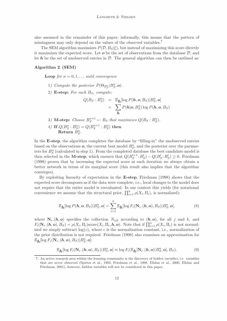
Langseth & Nielsen
also assumed in the remainder of this paper; informally, this means that the pattern ofmissingness may only depend on the values of the observed variables.7
The SEM algorithm maximizes P (D, BS |ξ), but instead of maximizing this score directlyit maximizes the expected score. Let o be the set of observations from the database D, andlet h be the set of unobserved entries in D. The general algorithm can then be outlined as:
Algorithm 2 (SEM)
Loop for n = 0, 1, . . . until convergence
1) Compute the posterior P (ΘBnS|Bn
S ,o).
2) E-step: For each BS, compute:
Q(BS : BnS) = Eh[log P (h,o, BS)|Bn
S ,o]
=∑h
P (h|o, BnS) log P (h,o, BS)
3) M-step: Choose Bn+1S ← BS that maximizes Q(BS : Bn
S).
4) If Q(BnS : Bn
S) = Q(Bn+1S : Bn
S) thenReturn Bn
S.
In the E-step, the algorithm completes the database by “filling-in” the unobserved entriesbased on the observations o, the current best model Bn
S , and the posterior over the parame-ters for Bn
S (calculated in step 1). From the completed database the best candidate model isthen selected in the M-step, which ensures that Q(Bl+1
S :BlS)−Q(Bl
S :BlS) ≥ 0. Friedman
(1998) proves that by increasing the expected score at each iteration we always obtain abetter network in terms of its marginal score (this result also implies that the algorithmconverges).
By exploiting linearity of expectation in the E-step, Friedman (1998) shows that theexpected score decomposes as if the data were complete, i.e., local changes to the model doesnot require that the entire model is reevaluated. In our context this yields (for notationalconvenience we assume that the structural prior,
∏ni=1 ρ(Xi,Πi), is normalized):
Eh[log P (h,o, BS)|BnS ,o] =
n∑i=1
Eh[log Fi(Ni··(h,o), BS)|BnS ,o], (8)
where Ni··(h,o) specifies the collection Nijk according to (h,o), for all j and k, andFi(Ni··(h,o), BS) = ρ(Xi,Πi)score(Xi,Πi,h,o). Note that if
∏ni=1 ρ(Xi,Πi) is not normal-
ized we simply subtract log(c), where c is the normalization constant, i.e., normalization ofthe prior distribution is not required. Friedman (1998) also examines an approximation forEh[log Fi(Ni··(h,o), BS)|Bn
S ,o]:
Eh[log Fi(Ni··(h,o), BS)|BnS ,o] ≈ log Fi(Eh[Ni··(h,o)|Bn
S ,o], BS). (9)
7. An active research area within the learning community is the discovery of hidden variables, i.e. variablesthat are never observed (Spirtes et al., 1993, Friedman et al., 1998, Elidan et al., 2000, Elidan andFriedman, 2001), however, hidden variables will not be considered in this paper.
12

Knowledge Fusion for Structural Learning in OO Domains
The approximation is exact if log Fi is linear in its arguments; this is, however, not the casewhen using the BD or BDe metric.8 Finally, the term Eh[Ni··(h,o)|Bn
S ,o] can be computedas:
∀j, k : Eh[Nijk(h,o)|BnS ,o] =
N∑l=1
P (Xi = k,Πi = j|Dl, BnS).
3.4 Learning dynamic Bayesian networks
Friedman et al. (1998) describe an algorithm for learning DBNs from both complete andincomplete data. The methods proposed in (Friedman et al., 1998) extend both the BayesianInformation Criterion (BIC) and the BDe score for learning DBNs from complete data; whenlifting the assumption that the database is complete, Friedman et al. (1998) extend the SEMalgorithm accordingly.
Friedman et al. (1998) define a DBN by partitioning the variables into time-slices s.t.the variables which occur at time t are denoted X[t]. Thus, a DBN with l time-slicesconsists of the variables X[0]∪X[1]∪ · · · ∪X[l]. It is assumed that the DBN is Markovian,i.e., P (X[t + 1]|X [0], . . . ,X[t]) = P (X [t + 1]|X [t]). By also assuming that the DBN isstationary (the CPTs associated with the variables in X [t] are independent of t, for t > 0),a DBN can be completely described by two parts: i) An initial network, B0, that specifiesa distribution over X[0] and ii) a transition network, B→, over the variables X[0] ∪X[1].
In the context of DBNs, the database is assumed to consist of N cases, where the m’thcase specifies a configuration over the variables X[0]∪X[1]∪ · · · ∪X[l]. Now, consider thesituation where the database is complete and let θ0
ij′k and θ→ijk be defined as in Section 3.1for B0 and B→, respectively; we use j′ and j to indicate that the parents for Xi maybe different in B0 and B→. Additionally, let the sufficient statistics be given by N0
ij′k =∑Nm=1 γ(Xi[0] = k,Πi = j′ : Dm) and N→
ijk =∑l
t=1
∑Nm=1 γ(Xi[t] = k,Πi = j : Dm).
By derivations similar to those of the BD metric, the following closed form expression forP (D, (B0, B→)|ξ) is obtained:
P (D, (B0, B→)|ξ) = P ((B0, B→)|ξ)
· n∏
i=1
q′i∏j′=1
Γ(N′0ij′)
Γ(N0ij′ + N
′0ij′)
ri∏k=1
Γ(N0ij′k + N
′0ij′k)
Γ(N ′0ij′k)
· n∏
i=1
qi∏j=1
Γ(N′→ij )
Γ(N→ij + N
′→ij )
ri∏k=1
Γ(N→ijk + N
′→ijk )
Γ(N ′→ijk )
.
Note that when maximizing this expression we can consider the two terms independentlyassuming that P (B0, B→|ξ) = P (B0|ξ) · P (B→|ξ).
Friedman et al. (1998) overcome the problem of specifying the virtual counts for thecandidate network structures by advocating the method of Heckerman et al. (1995). Thatis, given a prior DBN Bp = (B0
p , B→p ) and two equivalent sample sizes for B0
p and B→p , the
virtual counts are found as in Equation 6.
8. Friedman (1998) shows that the error of the linear approximation vanishes as the size of the databaseapproaches infinity.
13

Langseth & Nielsen
4. Specifying prior information
When learning a Bayesian network, the prior information about the domain is representedby i) a prior distribution over the discrete space of all candidate structures, and ii) a priordistribution over the continuous space of probability parameters for each model. In Section3.2 we briefly described a prior for the probability parameters, and in this section we willfocus on the use of prior information regarding the structure of BNs and OOBNs.
4.1 Structural priors in BNs
The use of structural priors when learning BNs has received only little attention in thelearning community. The most obvious reason is that in most cases the effect of the prioris dominated by the likelihood term, even for relatively small databases. One exception,however, is when some of the network structures are given zero probability a priori, in whichcase the data cannot change that belief.
Common to most (if not all) structural priors proposed in the literature is that theyobey the structural modularity assumption (see Section 3.2):
P (BS | ξ) ∝n∏
i=1
ρ(Xi,Πi) .
That is, the prior decomposes into a product with one term for each family in the networkstructure. This assumption ensures that during structure search (given complete data – ordata “completed” by the SEM algorithm) we can compare two candidate structures by onlyconsidering the local scores and priors for the families for which they differ.
Because of their relatively small influence upon the selected model, structural priorsare most often used to encode ignorance, and in some cases to restrict model complexity.Examples include the uniform prior ρ(Xi,Πi) = 1 (Cooper and Herskovits, 1991), and
ρ(Xi,Πi) =(
n− 1|Πi |
)−1
used in e.g. (Friedman and Koller, 2000). Another prior which is frequently used is ρ(Xi,Πi)= κδi (Heckerman et al., 1995), where 0 < κ ≤ 1 and
δi = | Πi(BS) ∪Πi(Bp) \ Πi(BS) ∩Πi(Bp) |
denotes the number of parents for Xi that differs in the prior model Bp and the candidatestructure BS . Thus, each such parent is penalized by a constant κ. The flexibility of thisprior can easily be extended by setting
δi =∑j 6=i
(ω+ij δ+
ij + ω−ij δ−ij) , (10)
where δ+ij is 1 if there is an edge from Xj to Xi in the candidate structure but not in the prior
model, and 0 otherwise; δ−ij is 1 if there is an edge from Xj to Xi in the prior model, but notin BS , and 0 otherwise. (ω+
ij , ω−ij) ∈ R
+×R+ is a pair of weights that indicates how certain
14
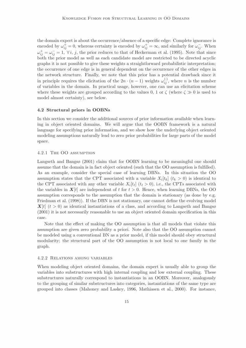
Knowledge Fusion for Structural Learning in OO Domains
the domain expert is about the occurrence/absence of a specific edge: Complete ignorance isencoded by ω+
ij = 0, whereas certainty is encoded by ω+ij =∞, and similarly for ω−
ij . Whenω+
ij = ω−ij = 1, ∀ i, j, the prior reduces to that of Heckerman et al. (1995). Note that since
both the prior model as well as each candidate model are restricted to be directed acyclicgraphs it is not possible to give these weights a straightforward probabilistic interpretation;the occurrence of one edge is in general dependent on the occurrence of the other edges inthe network structure. Finally, we note that this prior has a potential drawback since itin principle requires the elicitation of the 2n · (n − 1) weights ω
(·)ij , where n is the number
of variables in the domain. In practical usage, however, one can use an elicitation schemewhere these weights are grouped according to the values 0, 1 or ζ (where ζ 0 is used tomodel almost certainty), see below.
4.2 Structural priors in OOBNs
In this section we consider the additional sources of prior information available when learn-ing in object oriented domains. We will argue that the OOBN framework is a naturallanguage for specifying prior information, and we show how the underlying object orientedmodeling assumptions naturally lead to zero prior probabilities for large parts of the modelspace.
4.2.1 The OO assumption
Langseth and Bangsø (2001) claim that for OOBN learning to be meaningful one shouldassume that the domain is in fact object oriented (such that the OO assumption is fulfilled).As an example, consider the special case of learning DBNs. In this situation the OOassumption states that the CPT associated with a variable Xi[tk] (tk > 0) is identical tothe CPT associated with any other variable Xi[t`] (t` > 0), i.e., the CPTs associated withthe variables in X[t] are independent of t for t > 0. Hence, when learning DBNs, the OOassumption corresponds to the assumption that the domain is stationary (as done by e.g.Friedman et al. (1998)). If the DBN is not stationary, one cannot define the evolving modelX[t] (t > 0) as identical instantiations of a class, and according to Langseth and Bangsø(2001) it is not necessarily reasonable to use an object oriented domain specification in thiscase.
Note that the effect of making the OO assumption is that all models that violate thisassumption are given zero probability a priori. Note also that the OO assumption cannotbe modeled using a conventional BN as a prior model, if this model should obey structuralmodularity; the structural part of the OO assumption is not local to one family in thegraph.
4.2.2 Relations among variables
When modeling object oriented domains, the domain expert is usually able to group thevariables into substructures with high internal coupling and low external coupling. Thesesubstructures naturally correspond to instantiations in an OOBN. Moreover, analogouslyto the grouping of similar substructures into categories, instantiations of the same type aregrouped into classes (Mahoney and Laskey, 1996, Mathiasen et al., 2000). For instance,
15
Langseth & Nielsen
a set of substructures may correspond to the same type of physical object or they maydescribe a set of entities that occur at the same instant of time.
Such types of prior information can be represented by a (partial) OOBN specification(i.e. a prior model). The a priori specification of an OOBN contains a list of class speci-fications and a grouping of the nodes into instantiations which are classified according tothe classes. This prior OOBN model can then be used as in the case of conventional priormodels, and we can in principle use any of the definitions of ρ(Xi,Πi) outlined above.
When specifying the relations among the variables, it may be difficult for the domainexpert to indicate the presence or absence of edges between specific nodes in the model.If, for example, two variables X and Y in an instantiation I are strongly correlated, thedomain expert may be uncertain whether another node Z in the encapsulating context ofI should be the parent of X or Y , even though he believes that Z should influence at leastone of them. In the OOBN framework, this prior information can be encoded by specifyingthe interface between the instantiation I and its encapsulating context. For instance, thedomain expert can indicate which instantiations are allowed (and more importantly, denied)to reference a particular node (see Figure 8). Specifically, the domain expert could be askedquestions like “Do you think it is possible that a variable Z directly influences any of thevariables in instantiation I?”
Z
X Y
W
I:C
Figure 8: The figure depicts a possible way to describe knowledge about the structure ofthe domain; it shows an instantiation I and some of its encapsulating context(note that this is not strictly speaking an OOBN).
The use of such prior models is also supported by Equation 10, since edges that are notconsidered possible a priori are penalized strongly (ω+
ij = ζ 0). On the other hand, theinterface of an instantiation defines edges from a single node to a group of nodes hence,missing reference links cannot be penalized (as the prior specification at the class levelshould obey structural modularity), and we therefore use ω−
ij = 0. As an example, seeFigure 8, where we assume that the instantiation I consists of the two nodes X and Y ,and that (a priori) only Z is regarded as a possible node to be referenced from I. Fromthe discussion above, it follows that a candidate network where no node is referenced fromI will not be penalized by this prior, because ω−
XZ = ω−Y Z = 0. If we were to use a prior
which penalizes the “missing” link between Z and the instantiation I, then this prior wouldhave to encode that the probability for a link between Z and X depends on the existenceof a link between Z and Y ; the prior only penalizes a link missing between Z and X ifthere is no link from Z to Y . This violates structural modularity, which says that the priorshould factorize into a product of terms, where each term only depends on one family in
16
Knowledge Fusion for Structural Learning in OO Domains
the graph, see Section 3.2. On the other hand, if a candidate model is designed so thatanother node, say W , is referenced from I, it will be given a lower a priori belief (becauseω+
XW = ω+Y W = ζ). Note that the OOBN framework is not required to model this vague
prior information; it is merely a straight forward usage of Equation 10. However, to elicitsuch information it turns out to be useful to have grouped the nodes into what correspondsto instantiations, and then focus on the interfaces of these, i.e., to work in the frameworkof OOBNs.
To verify the ease of determining the interfaces a priori we conducted an experimentamongst our co-workers: The task was to identify the interfaces of the instantiations inthe object oriented version of the insurance domain, see Section 2.2. The test-persons werefamiliar with the OOBN framework, but they had not seen the insurance network before.Initially they were given the object oriented version of the insurance network, where eachnode was allocated to one of the instantiations (with all edges removed). The task wasthen to identify the interface of all instantiations in the domain, simply by indicating whichnodes inside an instantiation Ii could (possibly) be referenced from an instantiation Ij. Thetest-persons had no other information about the domain, except for what they were able todeduce from the names of the nodes. They where guided through the knowledge acquisitionby questions of the type “Is it possible that a person’s Age can directly influence any of thenodes in the instantiation of the Driver-class (RiskAversion, SeniorTrain, DrivingSkill,DrivQuality or DrivHist)?” The result of the experiment was that out of the 702 edges thatcan be included in the model, only 253 were marked possible. All the 52 edges actually inthe model were considered legal. The elicitation of this information took about 10 minutes;this result at least suggests that the approach is promising.
5. Learning in OOBNs
In this section we describe a method for learning in object oriented domains, casted as theproblem of finding the maximum a posteriori OOBN structure given a database D.
The basic idea of the object oriented learning method resembles that of Langseth andBangsø (2001) who utilizes the OO assumption when learning the parameters in an OOBN.Specifically, based on this assumption, Langseth and Bangsø (2001) propose to learn at theclass level of the OOBN instead of in the underlying BN; cases from the instantiations ofa class are considered (virtual) cases of that class.9 Langseth and Bangsø (2001) give boththeoretical as well as empirical evidence that this learning method is superior to conventionalparameter learning in object oriented domains.
5.1 Structural OO learning
The goal of our learning algorithm is to find a good estimate of the unknown underlyingstatistical distribution function, i.e., the task of density estimation (Silverman, 1986). Notethat if focus had been on e.g. causal discovery (Heckerman, 1995a), classification (Friedmanet al., 1997a), or generating a model that was able to predict well according to a predefined
9. Note that this approach can be seen as a generalization of the method for parameter learning in DBNs,see e.g. (West and Harrison, 1997).
17
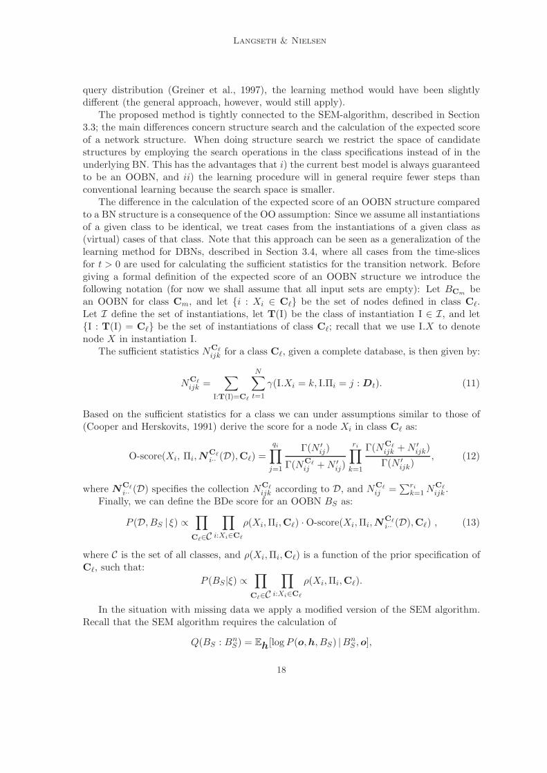
Langseth & Nielsen
query distribution (Greiner et al., 1997), the learning method would have been slightlydifferent (the general approach, however, would still apply).
The proposed method is tightly connected to the SEM-algorithm, described in Section3.3; the main differences concern structure search and the calculation of the expected scoreof a network structure. When doing structure search we restrict the space of candidatestructures by employing the search operations in the class specifications instead of in theunderlying BN. This has the advantages that i) the current best model is always guaranteedto be an OOBN, and ii) the learning procedure will in general require fewer steps thanconventional learning because the search space is smaller.
The difference in the calculation of the expected score of an OOBN structure comparedto a BN structure is a consequence of the OO assumption: Since we assume all instantiationsof a given class to be identical, we treat cases from the instantiations of a given class as(virtual) cases of that class. Note that this approach can be seen as a generalization of thelearning method for DBNs, described in Section 3.4, where all cases from the time-slicesfor t > 0 are used for calculating the sufficient statistics for the transition network. Beforegiving a formal definition of the expected score of an OOBN structure we introduce thefollowing notation (for now we shall assume that all input sets are empty): Let BCm bean OOBN for class Cm, and let i : Xi ∈ C` be the set of nodes defined in class C`.Let I define the set of instantiations, let T(I) be the class of instantiation I ∈ I, and letI : T(I) = C` be the set of instantiations of class C`; recall that we use I.X to denotenode X in instantiation I.
The sufficient statistics NC`ijk for a class C`, given a complete database, is then given by:
NC`ijk =
∑I:T(I)=C`
N∑t=1
γ(I.Xi = k, I.Πi = j : Dt). (11)
Based on the sufficient statistics for a class we can under assumptions similar to those of(Cooper and Herskovits, 1991) derive the score for a node Xi in class C` as:
O-score(Xi, Πi,NC`i·· (D),C`) =
qi∏j=1
Γ(N ′ij)
Γ(NC`ij + N ′
ij)
ri∏k=1
Γ(NC`ijk + N ′
ijk)
Γ(N ′ijk)
, (12)
where NC`i·· (D) specifies the collection NC`
ijk according to D, and NC`ij =
∑rik=1 NC`
ijk .Finally, we can define the BDe score for an OOBN BS as:
P (D, BS | ξ) ∝∏
C`∈C
∏i:Xi∈C`
ρ(Xi,Πi,C`) ·O-score(Xi,Πi,NC`i·· (D),C`) , (13)
where C is the set of all classes, and ρ(Xi,Πi,C`) is a function of the prior specification ofC`, such that:
P (BS |ξ) ∝∏
C`∈C
∏i:Xi∈C`
ρ(Xi,Πi,C`).
In the situation with missing data we apply a modified version of the SEM algorithm.Recall that the SEM algorithm requires the calculation of
Q(BS : BnS) = Eh[log P (o,h, BS) |Bn
S ,o],
18

Knowledge Fusion for Structural Learning in OO Domains
where o and h denote the observed and unobserved entries in D, respectively, and BnS is
the current best model. In accordance with Equation 8 and Equation 13 we have (again weassume that the prior distribution is normalized):
Eh[log P (o,h, BS) |BnS ,o] =
∑C`∈C
∑i:Xi∈C`
Eh[log Fi,C`(NC`
i·· (h,o), BS)|BnS ,o] (14)
where
Fi,C`(NC`
i·· (h,o), BS) = ρ(Xi,Πi,C`) ·O-score(Xi,Πi,NC`i·· (h,o),C`).
Now, analogously to the SEM algorithm we advocate the approximation proposed in Equa-tion 9 hence, for an OOBN we approximate:
Eh[log Fi,C`(NC`
i·· (h,o), BS)|BnS ,o] ≈ log Fi,C`
(Eh[NC`i·· (h,o)|Bn
S ,o], BS).
Finally, the expected counts Eh[NC`i·· (h,o)|Bn
S ,o] for node Xi in class C` is given by:
∀j, k : Eh[NC`ijk(h,o)|Bn
S ,o] =∑
I:T(I)=C`
N∑t=1
P (I.Xi = k, I.Πi = j |Dt, BnS).
Now, both Q(BS :BnS) and the posterior P (D, BS | ξ) factorizes over the variables (and
therefore also over the classes). Hence, in order to compare two candidate structures whichonly differ w.r.t. the edge Xi → Xj we only need to re-calculate the score (Equation 12)and ρ(Xj ,Πj ,C`) for node Xj in the class C` where Xj is defined. Note that this propertyalso supports the proposed search procedure which is employed at the class level.
Unfortunately, this type of locality to a class is violated when the input sets are non-empty (this is for instance the case with the two instantiations of the class Milk Cow thatare embedded in the Stock class). The problem occurs when new input nodes are added toa class interface, since the search for a “good” set of parents is not necessarily local to a classwhen the interface is not given; recall that the actual nodes included through the interfaceof an instantiation is not defined in the class specification, but locally in each instantiation.This may result in a serious computational overhead when determining the interface sincewe require that the OO assumption is satisfied. As an example, assume that the node X ininstantiation Ii is assigned an input node Y ′ as parent, and assume that Y ′ references thenode Y . Then, due to the OO assumption, the algorithm should find a node Z that hasthe same influence on Ij.X as Y has on Ii.X, for all instantiations Ij where T(Ij) = T(Ii).The search for Z must cover all nodes in the encapsulating context of Ij; note that Z maybe non-existent in which case the default potential for the input node should be used. Thecomplexity of finding the best candidate interface for all instantiations is exponential in thenumber of instantiations, and we risk using a non-negligible amount of time to evaluatenetwork structures with low score, e.g., if Y ′ (or more precisely the node Y referenced byY ′) is actually not needed as a parent for Ii.X.
To overcome this computational difficulty we propose the following algorithm which isinspired by the SEM algorithm (Algorithm 2). Basically, the algorithm iteratively learnsa) the interfaces of the instantiations by keeping the structure inside the instantiations
19

Langseth & Nielsen
fixed according to the classes (Step i and ii), and b) learns the structure inside each classbased on the candidate interfaces found in the previous steps (Step iii). Observe that Step3 corresponds to the E-step in the SEM algorithm and that Step 4 corresponds to theM-step.
Algorithm 3 (OO–SEM)
a) Let B0S be the prior OOBN model.
b) Loop for n = 0, 1, . . . until convergence
1) Compute the posterior P (ΘBnS|Bn
S ,o), see (Langseth and Bangsø, 2001) and(Green, 1990).
2) Set Bn,0S ← Bn
S.
3) For i = 0, 1, . . .
i) Let BS be the model which is obtained from Bn,iS by employing either none or
exactly one of the operations add-edge and remove-edge, for each instantia-tion I; each edge involved must have a node in both I and in the encapsulatingcontext of I (directed into I). The OO assumption is disregarded.10
ii) For each node X which is a child of an input node Y ′ (found in step (i))in instantiation Ij , determine if Ik.X has an input node as parent with thesame state space as Y ′, for all k 6= j where T(Ik) = T(Ij). If this is thecase, use the BDe score to determine if they should be assigned the sameCPT (due to the OO assumption); otherwise introduce default potentials toensure that they have the same CPTs.11 Let B′
S be the resulting network.iii) For each class C` in B′
S employ the operations add-edge or remove-edgew.r.t. the nodes in the class (excluding the input set) based on the candidateinterface found in step (ii). Note that edges from instantiations encapsulatedin C` into nodes defined in C` are also considered in this step.12 Let B′′
S bethe resulting OOBN.
iv) Set Bn,i+1S ← B′′
S.
4) Choose Bn+1S ← Bn,i
S that maximizes Q(Bn,iS : Bn
S) (Equation 14).
5) If Q(BnS : Bn
S) = Q(Bn+1S : Bn
S) thenReturn Bn
S .
Note that in Step (ii) it may seem counterintuitive to compare CPTs using the BDe score,however, observe that this step is actually used to restrict the parameter space and the BDescore is therefore appropriate, cf. the discussion in Section 3.
10. The number of operations is bounded by the product of the number of nodes in I and the number of nodesin the encapsulating context, but only the terms local to the involved families need to be re-calculated.
11. The CPTs are estimated by setting θC`ijk =
(NC`
ijk + N ′ijk
)/
(NC`
ij + N ′ij
), where NC`
ijk is the expected
sufficient statistics calculated according to Equation 11. Note that introducing default potentials haveno effect on the underlying BN (they can just be marginalized out).
12. An example of this situation is illustrated in Figure 6, where an instantiation of Driver is encapsulated inthe class CarOwner; observe that only the terms local to the involved families need to be re-calculated.
20

Knowledge Fusion for Structural Learning in OO Domains
In case of a complete database, the outer loop is simply evaluated once; evaluating thenetwork structures using Q(BS : Bn
S) is identical to using the BDe score for OOBNs in thiscase.
Theorem 1 Let D be a complete database of size N generated by an OOBN model withstructure B∗
S. If N → ∞, then the structure BS returned by Algorithm 3 is likelihoodequivalent to B∗
S.
Proof Notice that the space of OOBN structures is finite, and that each OOBN structurecan be visited by the inner loop of Algorithm 3. Note also that the greedy approach in step(ii) is asymptotically correct as the associated search space is uni-modal (as N →∞) andthe operations are transitive. From these observations the proof is straightforward as theBDe score is asymptotically correct, see (Heckerman, 1995b, Geiger et al., 1996).
Notice that the theorem above only holds when the database is complete; when the databaseis incomplete we have the following corollary.
Corollary 2 Let B0S , B1
S , . . . be the sequence of structures investigated by Algorithm 3, andlet D be a database. Then limn→∞ P (o, Bn
S) exists, and it is a local maximum of P (o, BS)when regarded as a function of BS.
Proof Follows immediately from (Friedman, 1998, Theorem 3.1 and Theorem 3.2) by ob-serving that a) the space of OOBN structures is finite and the variables in the domain havediscrete state spaces, and b) in Steps (i − iii) we are always sure to increase the expectedscore of the candidate model.
Observe that in order to complete the operational specification of Algorithm 3, we need asearch algorithm, e.g. simulated annealing, for investigation the candidate structures (Step(i) and Step (iii) constitute the choice points). Note also that in order to maximize the scorein Step (ii) we would in principle need to investigate the set of all subsets of instantiationsand nodes (which have an input node as parent). To avoid this computational problem weinstead consider the instantiations and nodes pairwise (randomly chosen). This still ensuresthat the expected score increases in each iteration, i.e., the algorithm will converge eventhough we apply hill-climbing in Step (ii), see also Corollary 2.
Finally it should be emphazised that the main computational problem of Algorithm3 is in establishing the interfaces of the instantiations hence, we propose to elicit priorinformation based on specific enquiries about the interfaces. For instance, the domainexpert can be asked to specify the nodes each instantiation is allowed to reference; asargued in Section 4.2 this is easily elicitated in an object oriented domain.
5.2 Type uncertainty
So far we have assumed that the domain expert is able to unambiguously classify eachinstantiation to a specific class. Unfortunately, however, this may not be realistic in real-world applications. Not being able to classify an instantiation is an example of what iscalled type uncertainty in (Pfeffer, 2000); the expert is uncertain about the type (or class inour terminology) of an instantiation. However, even though we may be unable to determine
21

Langseth & Nielsen
whether e.g. Cow1 is a Milk cow or a Meat cow, see Section 2, we would still like toemploy the learning algorithm using all available data.
When subject to type uncertainty the main problem is as follows. Consider the situationwhere we have two instantiations Ii and Ij whose classes are uncertain. Assume that bothIi and Ij are a priori classified as being instantiations of Ck, and assume that the data fromIi and Ij are somewhat different. If the data from Ii is initially used for learning in Ck, thenthe class specification for Ck is updated and the probability of Ij being an instantiationof Ck may therefore change. Thus, the probability of Ij belonging to Ck is dependent onthe classification of Ii. An immediate approach to overcome this problem is brute force,where we consider all possible combinations of allocating the uncertain instantiations to theclasses. However, this method is computationally very hard, and is not suited for practicalpurposes if the number of combinations of instantiations and classes is large; the complexityis O
(|C||I |
).
In what follows we propose an alternative algorithm for handling type uncertainty; weshall assume that the domain expert encodes his prior beliefs about the classification ofthe instantiations I as a distribution over the classes C (this also allows us to restrictour search in the class tree to specific subtrees, if the domain expert encodes his priorbelief in that way). Recall that the main problem with type uncertainty is that learn-ing can only be performed locally in a class specification if all instantiations are allocatedto a class (with certainty). This observation forms the basis for the following algorithm,which iteratively classifies the instantiations based on the MAP distribution over the clas-sifications of the instantiations. Note that since the learned model is dependent on theclassification of the uncertain instantiations, the algorithm maximizes the joint probabil-ity P (D, BS(T ),T ), where T = T(I); we use the notation BS(T ) to indicate that thelearned model is a function of the classifications. This probability can be computed asP (D, BS(T ),T ) = P (D|BS(T ),T )P (BS(T ) | T )P (T ) where BS(T ) is a model consistentwith the classification T . In the following we will let T denote the current estimate of theclassification T(I). Furthermore, we use T I ← C` to denote that the estimate of T(I) isset to C`, and we use T −I to denote the estimate of T(I \ I).Algorithm 4 (Type Uncertainty)
a) Initialization: Find the classification with maximum probability according to theprior distribution over the classifications P (T(I)), and classify the instantiations ac-cordingly. Let T 0
be this initial classification.
b) Loop for n = 0, 1, . . . until convergence
1) T ′ ← T n.
2) For each uncertain instantiation I:i) For each classification C of I s.t. P (T(I) = C) > 0:
A) Classify I as an instantiation of class C: T ′I ← C.
B) Learn the OOBN B′S(T ′
) for the current classification of all instanti-ations (Algorithm 3).13 Calculate the joint probability of the data, the
13. Note that only those parts of the domain that have been changed by the classification of I need to bere-learned.
22

Knowledge Fusion for Structural Learning in OO Domains
model B′S(T ′
) and T ′:
f(C)← P(D, B′
S(T ′), T ′)
.
ii) Classify I to the class maximizing the joint probabilityP (D, B′
S(T ′), T ′
) by keeping the classifications T(I \ I) fixed:T ′
I ← arg maxC:P (T(I)=C)>0 f(C).
3) Let T n+1 ← T ′and let Bn+1
S be the model found according to the classification
T n+1.
4) If P(D, Bn+1
S (T n+1), T n+1
)= P
(D, Bn
S(T n), T n
)then
Return BnS(T n
).
The algorithm attempts to maximize the joint probability P (D, BS(T ),T ) by iterativelymaximizing 1) P (D, BS(T n
), T n) over the models BS with the current classification T n
(Step B), and 2) P (D, BnS(T n
−I,T(I)), (T n
−I,T(I))) over T(I) given the classification T n
−I
(Step ii). This also implies that the algorithm converges to a (local) maximum.
6. Empirical study
In this section we describe a set of empirical tests, which have been conducted to verify theproposed learning method. First, Algorithm 3 was employed to learn the OOBN model ofthe insurance domain. This was done to identify the effect of prior information that is noteasily exploited when the domain is not regarded as object oriented. Secondly, Algorithm3 was employed on the stock domain to consider the effect of the OO assumption, andAlgorithm 4 was used to verify the method for type uncertainty calculations. Finally,Algorithm 3 was tested w.r.t. predictive accuracy in the insurance domain.
6.1 Setup of the empirical study
The goal of the empirical study was to evaluate whether or not the proposed learningmethods generate good estimates of the unknown statistical distribution. Let f(x|Θ) bethe unknown gold standard distribution; x is a configuration of the domain and Θ are theparameters. fN (x|ΦN ) (or simply fN ) will be used to denote the approximation of f(x|Θ)based on N cases from the database.
Since an estimated model may have other edges than the gold standard model, thelearned CPTs of ΦN may have other domains than the CPTs of Θ. Hence a global measurefor the difference between the gold standard model and the estimated model is required. Inthe tests performed, we have measured this difference by using the Kullback-Leibler (KL)divergence (Kullback and Leibler, 1951) between the gold standard model and the estimatedmodel. The KL divergence is defined as
D(
f || fN
)=
∑x
f(x|Θ) log
[f(x|Θ)
fN(x|ΦN )
]. (15)
There are many arguments for using this particular measurement for calculating thequality of the approximation, see (Cover and Thomas, 1991). One of them is the fact that
23

Langseth & Nielsen
the KL divergence bound the maximum error in the assessed probability for a particularevent A, (Whittaker, 1990, Proposition 4.3.7):
supA
∣∣∣∣∣∑x∈A
f(x |Θ)−∑x∈A
fN (x|ΦN )
∣∣∣∣∣ ≤√
12·D
(f || fN
).
Similar result for the maximal error of the estimated conditional distribution is derived in(van Engelen, 1997). These results have made the KL divergence the “distance measure”14
of choice in Bayesian network learning, see e.g. (Pearl, 1988, Lam and Bacchus, 1994,Heckerman et al., 1995, Friedman and Yakhini, 1996, Dasgupta, 1997, Friedman, 1998,Cowell et al., 1999).
The learning method was tested by randomly generating a database of size N from thegold standard model, where 25% of the data was missing completely at random15(Littleand Rubin, 1987, Heitjan and Basu, 1996); note that the proposed algorithms actually onlydepend on the assumption that the data is missing at random. It is also worth emphazisingthat all nodes in the underlying BN are observable in our tests (recall that input nodesare not part of the underlying BN as these nodes are merged with the referenced nodes,see Algorithm 1). The database was used as input to the structural learning algorithms.This was repeated a total of 50 times, with N varying from 100 to 10.000. In our tests weused Algorithm 3 with a maximum of 10 iterations (approximate convergence was typicallyreached in 4–5 iterations). In each iteration a simulated annealing with parameters T0 = 50,α = 100, β = 100, γ = 0.75 and δ = 220 (see (Heckerman et al., 1995) for notation) wasperformed; we refer the interested reader to (Myers et al., 1999) for additional discussionon stochastic search algorithms for learning Bayesian networks.
Observe that in the tests we do not consider the issue of running time. However, eventhough the proposed algorithms might seem more complex than the SEM algorithm (dueto the nested iterations) the search space is in fact smaller and we therefore expect that thealgorithm require fewer steps than the ordinary SEM algorithm, see also Section 5.
6.2 The empirical results
Consider again the OOBN version of the insurance network described in Section 2.2, andrecall the small experiment we performed in our research group to elicit object orientedprior information in this domain (described in Section 4.2). The goal of the experiment wasto find edges in the OOBN we could disregard a priori, and the result was that out of the702 edges that can be included in the network structure, only 253 were marked possible,including all the 52 edges actually in the network structure. Based on this experiment, weemployed the algorithm to examine to what extent this prior information could benefit thesearch algorithm.
The empirical results for the insurance domain is given in Figure 9a. The object orientedprior information regarding the interfaces was coded as absolutely certain (ω+
ij = ∞ if anedge Xi → Xj required a larger interface than given by the prior information). As expected,
14. The KL divergence is not a distance measure in the mathematical sense, as D ( f || g ) = D ( g || f ) doesnot hold in general. The term here is used in the everyday-meaning of the phrase.
15. Informally, missing completely at random means that the observability of a variable does not depend onthe value of any other variable (neither missing nor observed).
24

Knowledge Fusion for Structural Learning in OO Domains
0123456789
10
2000 4000 6000 8000 10000
KL
Size of training set
OO priorsConventional priors
00.5
11.5
22.5
33.5
44.5
5
2000 4000 6000 8000 10000
KL
Size of training set
OO priorsConventional priors
a) Insurance domain b) Stock domain
Figure 9: The KL divergence of the gold standard model vs. the generated models forthe two cases “Conventional priors” (ρ(Xi, Πi(BS)) = 1/65|Πi(BS) |) and “OOpriors”, where parts of the search-space violating the prior information regardingthe interfaces were disregarded.
the KL divergence decreases with the level of information available to the learning algorithm,such that the results based on the “OO priors” is superior to the ones based on “conventionalpriors” (i.e., the standard SEM algorithm) for smaller databases. The results seem to be atthe same level for large databases, say N > 8.000.
The second test was conducted to analyze the effect of making the OO assumption,and was based on the stock domain. This domain consists of 2 instantiations of the Meatcow class and 2 instantiations of the class Milk cow, and it was expected that knowingthat pairs of cows were identical would increase the learning speed; the results in Figure 9bclearly show this effect. Note that learning of DBNs (see Section 3.4) is simply a specialcase of OOBN learning, since any DBN can be modeled by the usage of two OOBN classes(see Sections 2 and 4.2). Hence, the results in (Friedman et al., 1998) can be regarded asthe effect of the OO assumption in that special case.
A test was also performed to verify the type uncertainty algorithm. The test wasbased on the stock domain, and we assumed that the domain expert was ignorant aboutthe classification of Cow1. We employed Algorithm 4 to this problem, and the resultsare shown in Figure 10, together with the results when consistently choosing the wrongclassification (Milk Cow) and when consistently choosing the correct classification (MeatCow) averaged over five runs. The results are fairly promising, as the algorithm was ableto build a model which is comparable to the correct classification. Note that this problemwas made fairly difficult, as can be seen from the difference in the KL divergence betweenthe correct and the wrong classifications in Figure 10; the domain used in (Langseth andBangsø, 2001) has been modified to make the differences between the classes sufficientlysmall for the problem to be challenging.16
16. When we used the domain as defined in (Langseth and Bangsø, 2001) we were able to classify theinstantiation correctly for databases as small as N = 10 observations.
25

Langseth & Nielsen
0
0.5
1
1.5
2
2.5
3
3.5
4
2000 4000 6000 8000 10000
KL
Size of training set
Type Uncertainty classificationCorrect classificationWrong classification
Figure 10: The KL divergence of the gold standard model vs. the generated models forthe three cases “Type uncertainty classification” (Algorithm 4), the results of“Correct classification” and “Wrong classification”.
Finally, a test was performed to compare the predictive performance of networks learnedusing Algorithm 3 and the SEM algorithm (Algorithm 2). We generated two databases fromthe insurance network; the databases consisted of 2000 and 8000 cases, respectively, and25% of the data was missing completely at random. For this specific situation we tried topredict the expected cost of insurance, i.e., the sum of the expected costs as indicated bythe variables ILiCist, MedCost and PropCost (we assumed that the utility was linear w.r.t.the monetary values). The expected costs in the learned networks was then compared tothe expected cost in the gold standard network. This was done 25.000 times in each net-work. The test-scenarios were sampled without missing values, but some of the variableswere subsequently removed; specifically, we removed the variables RiskAversion, Mileage,DrivingSkill, DrivQuality, Theft, Accident, Cushioning, ThisCarDam, OtherCarCost, This-CarCost, ILiCost, MedCost and PropCost. The results of the test is shown is Table 1, whichspecifies the relative absolute error of the predictions.
2000 cases, Algorithm 2 with uniform priors 0.492000 cases, Algorithm 3 with “OO priors” 0.248000 cases, Algorithm 2 with uniform priors 0.298000 cases, Algorithm 3 with “OO priors” 0.22
Table 1: The table shows the relative absolute error of the predictions for networks learnedusing the OO-SEM algorithm and the traditional SEM algorithm.
26

Knowledge Fusion for Structural Learning in OO Domains
The results show that the predictive performance of networks learned using Algorithm 3is superior to networks learned using the SEM algorithm for databases of 2000 cases.17
Similar to the results using the KL divergence, we see that for 8000 cases the predictiveperformance of the two networks are almost the same.
7. Conclusion
In this paper we have proposed a method for doing structural learning in object orienteddomains. The learning algorithm is based on the OOBN framework by (Bangsø and Wuil-lemin, 2000b), and has been implemented using a tailor-made version of the Structural EMalgorithm by Friedman (1998). The proposed learning algorithm exploits an intuitive wayof expressing prior information in object oriented domains, and it was shown to be moreefficient than conventional learning algorithms in this setting.
Although the proposed learning algorithm is set in the framework of Bayesian modelselection we conjecture that the general idea of learning in the class specifications, insteadof in the underlying BN, has a broader applicability. For instance, we expect the overallapproach to be applicable when learning OOBNs using constraint-based methods (Spirteset al., 1993, Steck and Tresp, 1996).
A related area of work is the framework of probabilistic relational models (PRMs) (Getooret al., 2001). A PRM specifies a probability model for classes of objects, which can then beused in multiple contexts. Getoor et al. (2001) describe how these models can be learnedfrom relational databases: as opposed to OOBNs the focus is on learning a PRM for aspecific context, instead of learning subnetworks (classes) that can be applied in differentcontexts. Somewhat similar to the proposed algorithms, Getoor et al. (2001) also performslearning at the class level, but avoids the problem of identifying the “input sets” as thecontext is known, see also (Taskar et al., 2001).
Acknowledgments
We would like to thank our colleagues at the Decision Support Systems group, AalborgUniversity, for interesting discussions and helpful comments. In particular, Olav Bangsøparticipated in the outset of this work (Bangsø et al., 2001). We would also like to thankHugin Expert (www.hugin.com) for giving us access to the Hugin Decision Engine whichforms the basis for our implementation. Finally, we would like to thank the anonymousreviewers for constructive comments and suggestions for improving the paper.
References
Olav Bangsø, Helge Langseth, and Thomas D. Nielsen. Structural learning in object orienteddomains. In Proceedings of the Fourteenth International Florida Artificial IntelligenceResearch Society Conference, pages 340–344. AAAI Press, 2001.
17. Note that due to this particular setup of the tests, it is not reasonable to argue about the generalpredictive performance of the learned networks.
27
Langseth & Nielsen
Olav Bangsø and Pierre-Henri Wuillemin. Object oriented Bayesian networks. A frameworkfor topdown specification of large Bayesian networks with repetitive structures. Techni-cal report CIT-87.2-00-obphw1, Department of Computer Science, Aalborg University,2000a.
Olav Bangsø and Pierre-Henri Wuillemin. Top-down construction and repetitive struc-tures representation in Bayesian networks. In Proceedings of the Thirteenth InternationalFlorida Artificial Intelligence Research Society Conference, pages 282–286. AAAI Press,2000b.
John Binder, Daphne Koller, Stuart Russell, and Keiji Kanazawa. Adaptive probabilisticnetworks with hidden variables. Machine Learning, 29(2–3):213–244, 1997.
Wray L. Buntine. A guide to the literature on learning probabilistic networks from data.IEEE Transactions on Knowledge and Data Engineering, 8:195–210, 1996.
Peter Cheeseman and John Stutz. Bayesian classification (AutoClass): Theory and results.In Advances in knowledge discovery and data mining, pages 153–180. AAAI/MIT Press,1996. ISBN 0-262-56097-6.
David M. Chichering and David Heckerman. Efficient approximations for the marginallikelihood of Bayesian networks with hidden variables. Machine Learning, 29(2–3):181–212, 1997.
Gregory F. Cooper and Edward Herskovits. A Bayesian method for constructing Bayesianbelief networks from databases. In Proceedings of the Seventh Conference on Uncertaintyin Artificial Intelligence, pages 86–94. Morgan Kaufmann Publishers, 1991.
Gregory F. Cooper and Edward Herskovits. A Bayesian method for the induction of prob-abilistic networks from data. Machine Learning, 9:309–347, 1992.
Thomas M. Cover and Joy A. Thomas. Elements of Information Theory. Wiley, New York,1991. ISBN 0-471-06259-6.
Robert G. Cowell, A. Phillip Dawid, Steffen L. Lauritzen, and David J. Spiegelhalter.Probabilistic Networks and Expert Systems. Statistics for Engineering and InformationSciences. Springer Verlag, New York, 1999. ISBN 0-387-98767-3.
Sanjoy Dasgupta. The sample complexity of learning fixed-structure Bayesian networks.Machine Learning, 29(2–3):165–180, 1997.
Arthur P. Dempster, Nan M. Laird, and Donald B. Rubin. Maximum likelihood fromincomplete data via the EM algorithm. Journal of the Royal Statistical Society, SeriesB, 39:1–38, 1977.
Gal Elidan and Nir Friedman. Learning the dimensionality of hidden variables. In Pro-ceedings of the Seventeenth Conference on Uncertainty of Artificial Intelligence, pages144–151. Morgan Kaufmann Publishers, 2001.
28

Knowledge Fusion for Structural Learning in OO Domains
Gal Elidan, Noam Lotner, Nir Friedman, and Daphne Koller. Discovering hidden variables:A structure-based approach. In Advances in Neural Information Processing Systems 13,pages 479–485. MIT Press, 2000.
Nir Friedman. The Bayesian structural EM algorithm. In Proceedings of the FourteenthConference on Uncertainty in Artificial Intelligence, pages 129–138. Morgan KaufmannPublishers, 1998.
Nir Friedman, Dan Geiger, and Moises Goldszmidt. Bayesian network classifiers. MachineLearning, 29(2–3):131–163, 1997a.
Nir Friedman, Lise Getoor, Daphne Koller, and Avi Pfeffer. Learning probabilistic rela-tional models. In Proceedings of the Sixteenth International Joint Conference on ArtificialIntelligence, pages 1300–1309. Morgan Kaufmann Publishers, 1999.
Nir Friedman, Moises Goldszmidt, David Heckerman, and Stuart Russell. Challenge: Whereis the impact of Bayesian networks in learning? In Proceedings of the Fifteenth Interna-tional Joint Conference on Artificial Intelligence. Morgan Kaufmann Publishers, 1997b.URL: http://www.cs.huji.ac.il/labs/compbio/Repository/.
Nir Friedman and Daphne Koller. Being Bayesian about network structure. In Proceedings ofthe Sixteenth Conference on Uncertainty in Artificial Intelligence, pages 201–210. MorganKaufmann Publishers, 2000. To appear in Machine Learning, 50(1–2), 2003.
Nir Friedman, Kevin P. Murphy, and Stuart Russell. Learning the structure of dynamicprobabilistic networks. In Proceedings of the Fourteenth Conference on Uncertainty inArtificial Intelligence, pages 139–147. Morgan Kaufmann Publishers, 1998.
Nir Friedman and Zohar Yakhini. On the sample complexity of learning Bayesian networks.In Proceedings of the Twelfth Conference on Uncertainty in Artificial Intelligence, pages274–282. Morgan Kaufmann Publishers, 1996.
Dan Geiger, David Heckerman, and Christopher Meek. Asymptotic model selection withhidden variables. In Proceedings of the Twelfth Conference on Uncertainty in ArtificialIntelligence, pages 283–290. Morgan Kaufmann Publishers, 1996.
Lise Getoor, Nir Friedman, Daphne Koller, and Avi Pfeffer. Learning probabilistic relationalmodels. In Relational Data Mining, pages 307–338. Springer Verlag, Berlin, Germany,2001. ISBN 3-540-42289-7. See also (Friedman et al., 1999).
Peter J. Green. On use of the EM algorithm for penalized likelihood estimation. Journalof the Royal Statistical Society, Series B, 52(3):443–452, 1990.
Russell Greiner, Adam J. Grove, and Dale Schuurmans. Learning Bayesian nets that per-form well. In Proceedings of the Thirteenth Conference on Uncertainty in Artificial In-telligence, pages 198–207. Morgan Kaufmann Publishers, 1997.
David Heckerman. A Bayesian approach to learning causal networks. Technical ReportMSR-TR-95-04, Microsoft Research, 1995a.
29

Langseth & Nielsen
David Heckerman. A tutorial on learning with Bayesian networks. Technical Report MSR-TR-95-06, Microsoft Research, 1995b.
David Heckerman, Dan Geiger, and David M. Chickering. Learning Bayesian networks:The combination of knowledge and statistical data. Machine Learning, 20(3):197–243,1995.
Daniel F. Heitjan and Srabashi Basu. Distinguishing “Missing At Random” and “MissingCompletely At Random”. The American Statistician, 50(3):207–213, 1996.
Finn V. Jensen. An introduction to Bayesian networks. UCL Press, London, UK, 1996.ISBN 1-857-28332-5.
Finn V. Jensen. Bayesian Networks and Decision Graphs. Springer Verlag, New York, 2001.ISBN 0-387-95259-4.
Uffe Kjærulff. A computational scheme for reasoning in dynamic probabilistic networks.In Proceedings of the Eighth Conference on Uncertainty in Artificial Intelligence, pages121–129. Morgan Kaufmann Publishers, 1992.
Daphne Koller and Avi Pfeffer. Object-oriented Bayesian networks. In Proceedings of theThirteenth Conference on Uncertainty in Artificial Intelligence, pages 302–313. MorganKaufmann Publishers, 1997.
Paul J. Krause. Learning probabilistic networks. The Knowledge Engineering Review, 13(4):321–351, 1998.
Solomon Kullback and Richard A. Leibler. On information and sufficiency. Annals ofMathematical Statistics, 22:79–86, 1951.
Wai Lam and Fahiem Bacchus. Learning Bayesian belief networks: An approach based onthe MDL principle. Computational Intelligence, 10(4):269–293, 1994.
Helge Langseth and Olav Bangsø. Parameter learning in object oriented Bayesian networks.Annals of Mathematics and Artificial Intelligence, 31(1/4):221–243, 2001.
Kathryn B. Laskey and Suzanne M. Mahoney. Network fragments: Representing knowledgefor constructing probabilistic models. In Proceedings of the Thirteenth Conference onUncertainty in Artificial Intelligence, pages 334–341. Morgan Kaufmann Publishers, 1997.
Roderick J. A. Little and Donald B. Rubin. Statistical Analysis with Missing Data. JohnWiley & Sons, 1987. ISBN: 0-471-80254-9.
Suzanne M. Mahoney and Kathryn B. Laskey. Network engineering for complef belief net-works. In Proceedings of the Twelfth Conference on Uncertainty in Artificial Intelligence,pages 389–396. Morgan Kaufmann Publishers, 1996.
Lars Mathiasen, Andreas Munk-Nielsen, Peter A. Nielsen, and Jan Stage. Object-orientedanalysis & design. Marko Publishing ApS, Aalborg, Denmark, 2000. ISBN 8-777-51150-6.
30

Knowledge Fusion for Structural Learning in OO Domains
James W. Myers, Kathryn B. Laskey, and Tod S. Levitt. Learning Bayesian networksfrom incomplete data with stochastic search algorithms. In Proceedings of the FifteenthConference on Uncertainty in Artificial Intelligence, pages 476–485. Morgan KaufmannPublishers, 1999.
Judea Pearl. Probabilistic Reasoning in Intelligent Systems: Networks of Plausible Inference.Morgan Kaufmann Publishers, San Mateo, CA., 1988. ISBN 0-934-61373-7.
Avrom J. Pfeffer. Probabilistic Reasoning for Complex Systems. Ph.D. thesis, StanfordUniversity, 2000.
Malcolm Pradhan, Gregory Provan, Blackford Middleton, and Max Henrion. Knowledge en-gineering for large belief networks. In Proceedings of the Tenth Conference on Uncertaintyin Artificial Intelligence, pages 484–490. Morgan Kaufmann Publishers, 1994.
Brian D. Ripley. Pattern Recognition and Neural Networks. Cambridge University Press,Cambridge, UK, 1996. ISBN 0-521-46086-7.
Jorma Rissanen. Stochastic complexity (with discussion). Journal of the Royal StatisticalSociety, 49(3):223–239 and 253–265, 1987.
Gideon Schwarz. Estimating the dimension of a model. Annals of Statistics, 6:461–464,1978.
Bernard W. Silverman. Density Estimation for Statistics and Data Analysis. Monographson statistics and applied probability. Chapman and Hall, London, UK, 1986. ISBN 0-412-24620-1.
Peter Spirtes, Clark Glymour, and Richard Scheines. Causation, Prediction, and Search.Springer Verlag, New York, 1993. ISBN 0-387-97979-4.
Harald Steck and Volker Tresp. Bayesian belief networks for data mining. In Proceedingsof the 2. Workshop on Data Mining und Data Warehousing als Grundlage modernerentscheidungsunterstutzender Systeme, pages 145–154, University of Magdeburg, Ger-many, 1996. ISBN 3-929-75726-5.
Benjamin Taskar, Eran Segal, and Daphne Koller. Probabilistic classification and clusteringin relational data. In Proceedings of the Seventeenth International Joint Conference onArtificial Intelligence, pages 870–876. Morgan Kaufmann Publishers, 2001.
Robert A. van Engelen. Approximating Bayesian belief networks by arc removal. IEEETransactions on Pattern Analysis and Machine Intelligence, 19(8):916–920, 1997.
Mike West and Jeff Harrison. Bayesian Forecasting and Dynamic Models. Springer Verlag,New York, 2nd edition, 1997. ISBN 0-387-94725-6.
Joe Whittaker. Graphical models in applied multivariate statistics. Wiley, Chichester, 1990.ISBN 0-471-91750-8.
31

Langseth & Nielsen
Yang Xiang and Finn V. Jensen. Inference in multiply sectioned Bayesian networks withextended Shafer-Shenoy and lazy propagation. In Proceedings of the Fifteenth Conferenceon Uncertainty in Artificial Intelligence, pages 680–687. Morgan Kaufmann Publishers,1999.
Yang Xiang, David Poole, and Michael P. Beddoes. Multiply sectioned Bayesian networksand junction forests for large knowledge-based systems. Computational Intelligence, 9(2):171–220, 1993.
32


