Bayesian Optimization with Inequality Constraints

Jacob R. Gardner1 gardner.jake@wustl.eduMatt J. Kusner1 mkusner@wustl.eduZhixiang (Eddie) Xu1 xuzx@cse.wustl.eduKilian Q. Weinberger1 kilian@wustl.eduJohn P. Cunningham2 jpc2181@columbia.edu1Washington University in St. Louis, 1 Brookings Dr., St. Louis, MO 63130

2Columbia University, 116th St and Broadway, New York, NY 10027

Abstract

Bayesian optimization is a powerful frame-work for minimizing expensive objectivefunctions while using very few function eval-uations. It has been successfully applied to avariety of problems, including hyperparam-eter tuning and experimental design. How-ever, this framework has not been extendedto the inequality-constrained optimizationsetting, particularly the setting in which eval-uating feasibility is just as expensive as eval-uating the objective. Here we present con-strained Bayesian optimization, which placesa prior distribution on both the objective andthe constraint functions. We evaluate ourmethod on simulated and real data, demon-strating that constrained Bayesian optimiza-tion can quickly find optimal and feasiblepoints, even when small feasible regions causestandard methods to fail.

1. Introduction

Bayesian optimization has become a popular toolto solve a variety of optimization problems wheretraditional numerical methods are insu�cient. Formany optimization problems, traditional global opti-mizers will e↵ectively find minima (Liberti & Maculan,2006; Zhigliavskii, 2008). However, these methods re-quire evaluating the objective function many times.Bayesian optimization is designed to deal specificallywith objective functions that are prohibitively expen-sive to compute repeatedly, and therefore must be eval-

Proceedings of the 31

stInternational Conference on Ma-

chine Learning, Beijing, China, 2014. JMLR: W&CP vol-ume 32. Copyright 2014 by the author(s).

uated as few times as possible. A popular applicationis hyperparameter tuning, where the task is to min-imize the validation error of a machine learning al-gorithm as a function of its hyperparameters (Snoeket al., 2012; Bardenet et al., 2013; Swersky et al., 2013).In this setting, evaluating the objective function (vali-dation error) requires training the machine learning al-gorithm and evaluating it on validation data. Anotherapplication is in experimental design, where the goalis to optimize the outcome of some laboratory experi-ment as a function of tunable parameters (Azimi et al.,2010b). In this setting, evaluating a specific parame-ter setting incurs the cost of the resources–materials,money, time, etc.–required to run the experiment.

In addition to expensive evaluations of the objectivefunction, many optimization programs have similarlyexpensive evaluations of constraint functions. For ex-ample, to speed up k-Nearest Neighbor classification(Cover & Hart, 1967), one may deploy data structuresfor approximate nearest neighbor search. The parame-ters of such data structures,e.g. locality sensitive hash-ing (LSH) (Gionis et al., 1999; Andoni & Indyk, 2006),represent a trade-o↵ between test time and test accu-racy. The goal of optimizing these hyperparametersis to minimize test time, while constraining test accu-racy: a parameter setting is only feasible if it achievesthe same accuracy as the exact model. Similarly, in theexperimental design setting, one may wish to maximizethe yield of a chemical process, subject to the con-straint that the amount of some unwanted byproductproduced is below a specific threshold. In computermicro-architecture, fine-tuning the particular specifi-cations of a CPU (e.g. L1-Cache size, branch predic-tor range, cycle time) needs to be carefully balancedto optimize CPU speed, while keeping the power usagestrictly within a pre-specified budget. The speed andpower usage of a particular configuration can only be

evaluated with expensive simulation of typical work-loads (Azizi et al., 2010). In all of these examples, thefeasibility of an experiment is not known until afterthe experiment had been completed, and thus feasibil-ity can not always be determined in advance. In thecontext of Bayesian optimization, we say that eval-uating feasibility in these cases is also prohibitivelyexpensive, often on the same order of expense as eval-uating the objective function. These problems are par-ticularly di�cult when the feasible region is relativelysmall, and it may be prohibitive to even find a feasibleexperiment, much less an optimal one.

In this paper, we extend the Bayesian optimiza-tion framework naturally to scenarios of optimiz-ing an expensive-to-evaluate function under equallyexpensive-to-evaluate constraints. We evaluate ourproposed framework on two simulation studies andtwo real world learning tasks, based on LSH hyperpa-rameter tuning (Gionis et al., 1999) and SVM modelcompression (Bucilu et al., 2006; Burges & Scholkopf,1997).

Across all experiments, we outperform uniform sam-pling (Bergstra & Bengio, 2012) on 13 out of 14datasets—including cases where uniform sampling failsto find even a single feasible experiment.

2. Background

To motivate constrained Bayesian optimization, we be-gin by presenting Bayesian optimization and the keyobject on which it relies, the Gaussian process.

2.1. Gaussian Processes

A Gaussian process is an uncountable collection ofrandom variables, any finite subset of which havea joint Gaussian distribution. A Gaussian processthus provides a distribution over functions `(·) ⇠GP (µ(·), k(·, ·)), parameterized by mean function µ(·)and covariance kernel k(·, ·), which are defined suchthat, for any pairs of input points x,x0 2 Rd, we have:

µ(x) = E[`(x)]

k(x,x0) = E[(`(x) � µ(x))(`(x0) � µ(x0))].

Given a set of input points X = {x1, ...,xn},the corresponding function evaluations `(X) ={`(x1), ..., `(xn)}, and some query point x, the jointGaussianity of all finite subsets implies:

`(X)`(x)

�

⇠ N✓

µ(X)µ(x)

�

,

k(X,X) k(X, x)k(x,X) k(x, x)

�◆

,

where we have (in the standard way) overloaded thefunctions `(·), µ(·), and k(·, ·) to include elementwise-

operation across their inputs. We then can calculatethe posterior distribution of `(·) at the query pointx, which we denote ˜(x) := p (`(x)|x,X, `(X)). Usingthe standard conditioning rules for Gaussian random

variables, we see ˜(x) ⇠ N⇣

µ`(x), ⌃`(x)⌘

, where:

µ`(x) = µ(x) + k(x,X)k(X,X)�1(`(X) � µ(X))

⌃`(x) = k(x, x) � k(x,X)k(X,X)�1k(X, x).

A full treatment of the use of Gaussian processes formachine learning is Rasmussen (2006). In the con-text of this work, the critical takeaway is that, givenobserved function values `(X) = {`(x1), ..., `(xn)}, weare able to update our posterior belief ˜(x) of the func-tion `(·) at any query point, with simple linear algebra.

2.2. Bayesian optimization

Bayesian optimization is a framework to solve pro-grams:

minx

`(x),

where the objective function `(x) is considered pro-hibitively expensive to evaluate over a large set of val-ues. Given this prohibitive expense, in the Bayesianformalism, the uncertainty of the objective `(·) acrossnot-yet-evaluated input points is modeled as a proba-bility distribution. Bayesian optimization models `(·)as a Gaussian process, which can be evaluated rela-tively cheaply and often (Brochu et al., 2010). At eachiteration the Gaussian process model is used to selectthe most promising candidate x⇤ for evaluation. Thecostly function ` is then only evaluated at `(x⇤) in thisiteration. Subsequently, the Gaussian process natu-rally updates its posterior belief ˜(·) with the new datapair (x⇤

, `(x⇤)), and that pair is added to the knowndata set T` = {(x1, `(x1)), ..., (xn, `(xn))}. This itera-tion can be repeated to iterate to an optimum.

The critical step is the selection of the candidate pointx⇤, which is done via an acquisition function thatenables active learning of the objective `(·) (Settles,2010). The performance of Bayesian optimization de-pends critically on the choice of acquisition function.A popular pick is the Expected improvement of a can-didate point (Jones et al., 1998; Mockus et al., 1978).Let x be some candidate point, and let ˜(x) be theGaussian process posterior distribution for `(x). Letx+ be the best point in T` (evaluated thus far), namely:

x+ = minx2T`

`(x).

Following Mockus et al. (1978), we then define the im-provement of the candidate point x as the decrease of

`(x) against `(x+), which due to our Gaussian processmodel is itself a random quantity:

I(x) = maxn

0, `(x+) � ˜(x))o

, (1)

and thus the expected improvement (EI) acquisitionfunction is the expectation over this truncated Gaus-sian variable:

EI(x) = Eh

I(x)|xi

. (2)

Mockus et al. (1978); Jones et al. (1998) derive an easy-to-compute closed form for the EI acquisition function:

EI(x) = ⌃`(x) (Z�(Z) + �(Z))

with: Z =µ`(x) � f(x+)

⌃`(x),

where � is the standard normal cumulative distribu-tion function, and � is the standard normal probabil-ity density function. In summary, the Gaussian pro-cess model within Bayesian optimization leads to thesimple acquisition function EI(x) that can be used toactively select candidate points.

3. Method

In this paper we extend Bayesian Optimization to in-corporate inequality constraints, allowing problems ofthe form

minc(x)�

`(x). (3)

where both `(x) and c(x) are the results of some ex-pensive experiment. These values may often be theresult of the same experiment, and so when we con-duct the experiment, we compute both the value of`(x) and that of c(x).

3.1. Constrained Acquisition Function

Adding inequality constraints to Bayesian optimiza-tion is most directly done via the EI acquisition func-tion, which needs to be modified in two ways. First,we augment our definition of x+ to be the feasiblepoint with the lowest function value observed in T .Second, we assign zero improvement to all infeasiblepoint. This leads to the following constrained improve-ment function for a candidate x:

IC(x) = �(x) max�

0, `(x+) � `(x)

= �(x)I(x)

where �(x) 2 {0, 1} is a feasibility indicator functionthat is 1 if c(x) �, and 0 otherwise.

Because c(x) and `(x) are both expensive to com-pute, we again use the Bayesian formalism to model

each with a conditionally independent Gaussian pro-cess, given x. During Bayesian optimization, after wehave picked a candidate x to run, we evaluate `(x) andplace (x, `(x)) in T` as previously, and we also nowevaluate c(x) and add (x, c(x)) to the set Tc, whichis then used to update the Gaussian process posteriorc(x) ⇠ N (µc(x), ⌃c(x)) as above.

With this model, our Gaussian process models the con-strained acquisition function as the random quantity:

IC(x) = �(x) maxn

0, `(x+) � ˜(x))o

= �(x)I(x),

where the quantity �(x) is a Bernoulli random vari-able with parameter:

PF (x) := Pr [c(x) �] =

Z �

�1p(c(x)|x, Tc)dc(x)

Conveniently, due to the marginal Gaussianity of c(x),the quantity PF (x) is a simple univariate Gaussiancumulative distribution function.

These steps completed, we now result with the expectedconstrained improvement acquisition function:

EIC(x) = Eh

IC(x)|xi

= Eh

�(x)I(x)|xi

= Eh

�(x)|xi

Eh

I(x)|xi

= PF (x)EI(x),

where the third equality comes from the conditionalindependence of c(x) and `(x), given x.

Thus the expected constrained improvement acqui-sition function EIC(x) is precisely the standard ex-pected improvement of x over the best feasible pointso far weighted by the probability that x is feasible.

It is worth noting that, while infeasible points arenever considered our best experiment, they are stilluseful to add to T` and Tc to improve the Gaussian pro-cess posteriors. Practically speaking, infeasible sam-ples help to determine the shape and descent directionsof c(x), allowing the Gaussian process to discern whichregions are more likely to be feasible without actuallysampling there. This property–that we do not needto sample in feasible regions to find them–will provehighly useful in cases where the feasible region is rel-atively small, and otherwise uniform sampling wouldhave di�culty finding these regions.

3.2. Multiple Inequality Constraints

It is possible to extend the above derivation to per-form Bayesian optimization with multiple inequality

constraints.min

c(x)⇤

f(x)

where c(x)= [c1(x), ..., ck(x)] and ⇤ = [�1, ..., �k]. Wesimply redefine �(x) as the Bernoulli random variable

with Eh

�(x)i

= p(c1(x) �1, ..., ck(x) �k), and

the remainder of the EIc(x) constrained acquisitionfunction is unchanged.

Note that p(c1(x) �1, ..., ck(x) �k) is a multi-variate Gaussian probability. In the simplest case, weassume the constraints are conditionally independentgiven x, which conveniently factorizes the probabilityas

Qki=1 p(ci(x)), a product of univariate Gaussian cu-

mulative distribution functions. In the case of depen-dent constraints, this multivariate Gaussian probabil-ity can be calculated with available numerical methods(Cunningham et al., 2011).

4. Results

We evaluate our cBO framework on two synthetic tasksand two real world applications. In all cases we com-pare cBO with function minimization by uniform sam-pling, an approach that is generally considered com-petitive (Bergstra & Bengio, 2012) and typically moree�cient than grid-searching (Bishop, 2006). Our im-plementation is written in MATLABTM . In orderto not introduce additional hyper-parameters throughthe Bayesian optimization, we apply the standard ap-proach to set all GP hyper-parameters on-the-fly withmaximum likelihood estimation (Rasmussen, 2006).We will release our code and all scripts to reproducethe results in this section at http://anonymized.

4.1. Simulation Function

For the purpose of visualizing our method, we firstevaluate it on two simulations with 2d objective andconstraint functions. Both cBO and uniform samplingwere allowed 30 evaluations of `(·) and c(·).

Simulation 1. For the first simulation, the objectivefunction is

`(x, y) = cos(2x) cos(y) + sin(x),

which we want to minimize subject to the constraint

c(x, y) = cos(x) cos(y) � sin(x) sin(y) 0.5.

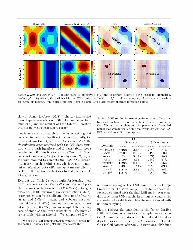
The upper row of figure 1 depicts the contour plotsof these functions, as well as the function evaluationsinitiated by the cBO optimization and uniform sam-pling. The infeasible regions are made opaque in the

two right plots. Black ⇥ symbols indicate infeasible lo-cations at which `(·) and c(·) were evaluated. Circles(black with white filling) indicate feasible evaluations.After a short amount of time, cBO narrows in on theglobal minimum of the constrained objective (the darkblue spot in the top right corner). In contrast, uniformsampling misses the optimum and wastes a lot of eval-uations (22/30) outside the feasible region (top rightplot). It is noteworthy that cBO also initiates multipleevaluations outside the feasible regions (14/30), how-ever these are very close to the global minimum (topright) or at the infeasible second minimum (dark bluespot at the bottom right), thus exploring the edge offeasibility where it matters the most.

Simulation 2. In the second simulation, we demon-strate how cBO can quickly find the minimum feasiblevalue of a function even when this feasible region isvery small. Here, the objective function (to be mini-mized) is

`(x, y) = sin(x),

subject to the constraint

c(x, y) = sin(x) sin(y) �0.95.

The results of this simulation are displayed in the lowerrow of figure 1. The feasible regions are small enoughthat uniform sampling might take some time to sam-ple a feasible point, and none of the 30 samples arefeasible. By contrast, cBO is quickly able to use infea-sible samples to su�ciently learn the constraint func-tion c(x, y) to locate the feasible regions. In addition,the infeasible samples are su�cient for cBO to learnto avoid the left half of the objective function, and themajority of samples are on the right half.

4.2. Locality Sensitive Hashing

As a first real world task, we evaluate cBO by selectingparameters for locality-sensitive hashing (LSH) (Gio-nis et al., 1999; Andoni & Indyk, 2006) for approximatek-nearest neighbors (kNN) (Cover & Hart, 1967). Webegin with a short description of LSH and the con-strained optimization problem. We then present theperformance of cBO alongside the uniform baseline.

Locality-sensitive hashing (LSH) is an approximatemethod for nearest neighbor search based on randomprojections. The overall intuition is that nearest neigh-bors always stay close after projections. LSH definesj random projections, or hash functions, h1, . . . , hj .This ‘hashing’ is performed multiple times, in sets of j

hash functions, and each set is called a hash table. Forfurther details we refer the interested reader to a re-

cBO Uniform Sampling

0 1 2 3 4 5 60

1

2

3

4

5

6

0 1 2 3 4 5 60

1

2

3

4

5

6

−0.8

−0.6

−0.4

−0.2

0

0.2

0.4

0.6

0.8

INFEASIBLE

INFEASIBLE

Objective `(x, y) Constraint function c(x, y)

0 1 2 3 4 5 60

1

2

3

4

5

6

−0.8

−0.6

−0.4

−0.2

0

0.2

0.4

0.6

0.8

0 1 2 3 4 5 60

1

2

3

4

5

6

−0.8

−0.6

−0.4

−0.2

0

0.2

0.4

0.6

0.8

INFEASIBLE INFEASIBLE

Sim

ulat

ion

1Si

mul

atio

n 2

INFEASIBLE

Figure 1. Left and center left: Contour plots of objective `(x, y) and constraint function c(x, y) used for simulation.center right: Bayesian optimization with the ECI acquisition function. right: uniform sampling. Areas shaded in whiteare infeasible regions. White circle indicate feasible points, and black crosses indicate infeasible points.

view by Slaney & Casey (2008).1 The key idea is thatthese hyper-parameters of LSH (the number of hashfunctions j and the number of hash tables L) create atradeo↵ between speed and accuracy.

Ideally, one wants to search for the fastest setting thatdoes not impact the classification error. Formally, theconstraint function c(j, L) is the leave-one-out (LOO)classification error obtained with the LSH data struc-ture with j hash functions and L hash tables. Let ✏

denote the LOO classification error without LSH. Thenour constraint is c(j, L) ✏. Our objective, `(j, L), isthe time required to compute the LOO kNN classifi-cation error on the training set, which we aim to min-imize. We allow both cBO and uniform sampling toperform 100 function evaluations to find such feasiblesettings of j and L.

Evaluation. Table 2 shows results for learning theseLSH parameters under the LOO constraint on 8 pop-ular datasets for face detection (YaleFaces) (Georghi-ades et al., 2001), insurance policy prediction (COIL),letter recognition from audio and font-specific features(Isolet and Letters), income and webpage classifica-tion (Adult and W8a), and optical character recog-nition (USPS, MNIST ). We subsampled the trainingdata of three of the larger datasets to 10% (markedin the table with an asterisk). We compare cBO with

1We use the LSH implementation from the Caltech Im-age Search Toolbox, http://tinyurl.com/caltechLSH.

Table 1. LSH results for selecting the number of hash ta-bles and functions for approximate kNN search. We showthe kNN evaluation time and the percentage of sampledpoints that were infeasible on 8 real-world datasets for BO-ECI, as well as uniform sampling.

LSHSpeedup % Infeasible

Dataset cBO Uniform cBO Uniform

yalefaces 6.08⇥ 3.97⇥ 25% 67%coil 32.0⇥ 8.17⇥ 61% 80%

isolet 4.70⇥ 5.18⇥ 50% 80%usps 4.10⇥ 3.03⇥ 27% 67%

letters 1.28⇥ 0.56⇥ 68% 96%adult* 8.63⇥ 1.34⇥ 70% 69%w8a* 3.27⇥ 2.85⇥ 60% 55%mnist* 1.87⇥ 1.42⇥ 52% 62%

uniform sampling of the LSH parameters (both op-timized over the same range). The table shows thespeedup obtained with the final LSH model over stan-dard Euclidean kNN search. In all but one case is thecBO-selected model faster than the one obtained withuniform sampling.

Figure 2 shows the traceplots of the fastest feasibleLSH kNN time as a function of sample iterations onthe Coil and Adult data sets. The red and blue dotsdepict iterations in which feasible points are selected.On the Coil dataset, after only 13 iterations, cBO finds

0 20 40 60 80 1000

1

2

3

4

5

6

7

cBOuniform

eval

uatio

n tim

e (s

econ

ds)

coil cBO

0 20 40 60 80 1000

1

2

3

4

5

6

7

8

9

iterations

adult

eval

uatio

n tim

e (s

econ

ds)

Figure 2. Plot of the best LSH nearest neighbor searchevaluation time (`) found so far versus iteration for cBOand uniform sampling on the Coil and Adult datasets.

a feasible setting of j and L that has a lower evaluationtime than any setting discovered by uniform sampling.On Adult, it is able to further decrease the evaluationtime from one that is similar to a setting eventuallyfound by uniform sampling.

Figure 3 shows a contour plot of the 2d objective sur-face on the USPS handwritten digits data set. Theinfeasible region is masked out in light blue. Fea-sible evaluation points are marked as white circles,whereas infeasible evaluations are denoted as blackcrosses. cBO queries only a few infeasible parametersettings and narrows in on the fastest model settings(dark blue feasible region). The majority of infeasiblepoints sampled are near the feasibility border (bottomleft). These points are nearly feasible and likely havelow objective. Because of this and the thin regions offeasibility, cBO explores this region with the hopes offurther minimizing `(·). Although uniform samplingdoes evaluate parameters near the optimum, the finalmodel only obtains a speedup of 3.03⇥ whereas cBO

returns a model with speedup 4.1⇥ (see Table 2).

4.3. SVM Compression

Our second real-world application is speeding up sup-port vector machines (SVM) (Cortes & Vapnik, 1995)through hyper-parameter search and support-vector“compression” (Burges & Scholkopf, 1997). In thiswork, Burges & Scholkopf (1997) describe a methodfor reducing the number of SVM support vectors usedfor the kernel support vector machine. Their approachis to first train a kernel SVM and record the learnedmodel and its predictions on the training set. Then,one selects an initial small subset of m support vectorsand re-optimizes them so that an SVM with only m

support vectors matches the predictions of the origi-nal model. This re-optimization can be done e�cientlywith conjugate gradient descent2 and can be very e↵ec-tive at speeding up SVMs during test-time—howeverit is highly dependent on several hyper-parameters andhas the potential to degrade a classifier’s performanceif done wrong.

We restrict our setting to the popular radial basis func-tion (RBF) kernel (Scholkopf & Smola, 2001),

k(x, z) = exp�

�

2kx� zk22�

, (4)

which is sensitive to a width parameter �

2. To speedup SVM evaluation we need to select values for �

2,the SVM cost parameter C, and the number of sup-port vectors m that minimize the validation evaluationtime. However, to avoid degrading the performance ofour classifier by using fewer support vectors, we needto constrain the validation error to increase by no morethan s% over the original SVM model.

To be precise, we first train an SVM on a particulardata set (all hyper-parameters are tuned with stan-dard Bayesian optimization). We then compress thismodel to minimize validation evaluation time, whileonly minimally a↵ecting its validation error (up to arelative increase of s%). For a particular parametersetting �

2, C, m, an evaluation of `() and c() involves

first compressing an SVM with parameters �

2, C down

to m support vectors following Burges & Scholkopf(1997), and then evaluating the resulting classifier onthe validation set. The value of `(�2

, C, m) is the timerequired for the evaluation (not the compression), andthe value of c(�2

, C, m) is the validation error. Thiserror is constrained to be no more than a factor 1 + s

larger than the validation error of the original SVM.As in the LSH task, we allow both cBO and uniformsampling to perform 100 evaluations.

2http://tinyurl.com/minimize-m

5 10 15 20

20

40

60

80

100

120

140

160

180

200

5 10 15 20

20

40

60

80

100

120

140

160

180

200cBO Uniform

Hash Functions j Hash Functions j

Has

h Fu

nctio

ns L

LSH

Sear

ch T

ime

(in s

econ

ds)

Figure 3. Contour plots of the kNN evaluation time on the USPS dataset using LSH with di↵erent number of hashtables L and hash functions j. The blue shaded region represents infeasible settings (based on the kNN error). Blackcrosses indicate infeasible points, white circles indicate feasible points. Left: Parameter settings evaluated by cBO. Right:Parameter settings evaluated by uniformly sampling.

Table 2. SVM compression results for selecting RBF hyperparameter �2, SVM cost hyperparameter C, and the number ofsupport vectors m. We show validation time and percent of points sampled that were infeasible by constrained Bayesianoptimization (Prob.) and uniform sampling.

1% relative error increase 10% relative error increaseNumber of Speedup ` % Infeasible SVs Speedup ` % Infeasible SVs

Dataset Samples cBO Uniform cBO Uniform cBO Uniform cBO Uniform cBO Uniform cBO Uniform

spam 3681 41⇥ 21⇥ 97% 99% 243 792 322⇥ 69⇥ 61% 74% 5 183magic* 1522 75⇥ 14⇥ 94% 95% 24 217 82⇥ 14⇥ 92% 95% 20 217adult* 3256 551⇥ 346⇥ 57% 25% 3 26 600⇥ 345⇥ 23% 1% 3 26w8a* 4975 156⇥ 98⇥ 31% 13% 3 64 155⇥ 98⇥ 27% 7% 3 64

ijcnn1* 4999 9.8⇥ � 99% 100% 836 � 9.8⇥ � 98% 100% 460 �forest* 5229 107⇥ � 98% 100% 294 � 208⇥ 26⇥ 93% 98% 101 1585

Comparison. Table 1 shows results for learning �

2,C and m on six medium scale UCI datasets3 includingspam classification (Spam), gamma particle and en-gine output detection (Magic and IJCNN1 ), and treetype identification (Forest). Similar to LSH, we sub-sampled the training data of four of the larger datasetsto 10% (marked in the table with an asterisk, the tableshows the data set size after subsampling). We con-sider the two cases of s = 1.01 and s = 1.1 relativevalidation error increase. The table presents the bestspeedups found by cBO and uniform sampling, the cor-responding number of support vectors (SVs), as wellas the percent of parameter settings that turned outto be infeasible. cBO outperforms uniform samplingon all datasets in speedup. In the most extreme case(Adult), the compressed SVM model was 551⇥ fasterthan the original with only 1% relative increase in val-idation error. On two data sets (IJCNN1 and Forest),uniform subsampling does not find a single compressedmodel that guarantees a validation error increase be-

3http://tinyurl.com/ucidatasets

low 1% (as well as 10% for IJCNN1). The table alsoshows the number of support vectors m, to which theSVM is compressed. In all cases is the cBO model sub-stantially smaller than the one obtained with uniformsampling.

One interesting observation is that uniform samplingfinds more feasible points for Adult and W8a datasets.A possible explanation for this is that a very fast pa-rameter setting is right near the feasibility border, sim-ilar to the case for LSH on the USPS dataset in Fig-ure 3 (Left). Indeed, it is likely for only m = 3 supportvectors many settings of �

2 and C will be infeasible.However, conBO was able to intelligently explore thefeasibility function until such a setting was found.

5. Related Work

There has been a large amount of recent work on usingsampling methods for blackbox optimization in ma-chine learning. A popular application of these methodsis hyperparameter tuning for machine learning algo-

rithms, or optimizing the validation performance of amachine learning algorithm as a function of its hyper-parameters. Bergstra & Bengio (2012) demonstratesthat uniform sampling performs significantly betterthan the common grid search approach. They proposethat the use of Bayesian optimization for this task ispromising, and uniform sampling serves as a baselinefor Bayesian optimization papers (Snoek et al., 2012).

A large number of Bayesian optimization papers havebeen published on the topic of hyperparameter tuningas well. Snoek et al. (2012) introduces Spearmint, apopular tool for this application. Spearmint marginal-izes over the Gaussian process hyperparameters usingslice sampling rather than finding the maximum likeli-hood hyperparameters. Spearmint also introduces theEI per cost acquisition function, which—in additionto its applications with costs other than time—oftenallows for faster optimization when some parametersa↵ect the running time of an experiment.

Spearmint also introduces a method for running manyexperiments in parallel by marginalizing over the pos-sible function values of pending experiments whencomputing the expected improvement of a new candi-date experiment. Parallelizing Bayesian optimizationis an active research area (Azimi et al., 2010a; 2012).

A few papers have also been published dealing withmulti task validation Bardenet et al. (2013); Swer-sky et al. (2013), where the goal is either to optimizemultiple datasets simultaneously, or use the knowl-edge gained from tuning previous datasets to providea warm start to the optimization of new datasets.

A number of papers have also been published apply-ing Bayesian optimization to other problems. Azimiet al. (2010b) extends Bayesian optimization to thecase where one cannot control the precise value ofsome parameters in an experiment. Mahendran et al.(2012) applies Bayesian optimization to perform adap-tive MCMC. Wang et al. (2013) adapts Bayesian opti-mization to very high dimensional settings. Finally,Ho↵man et al. (2013) introduce constraints on thenumber of function evaluations, rather than expensive-to-compute constraints, which we model with cBO.

6. Discussion

In conclusion, in this paper we extended BayesianOptimization to incorporate expensive to evaluate in-equality constraints. We believe this algorithm hasthe potential to gain traction in the machine learningcommunity and become a practical and valuable tool.Classical Bayesian optimization provides an excellentmeans to get the most out of many machine learn-

ing algorithms. However, there are many algorithms–particularly approximate algorithms with the goal ofspeed–that the standard Bayesian optimization frame-work is ill-suited to optimize. This is because it has noway of dealing with the fundamental tradeo↵ betweenspeed and accuracy that these algorithms present.

We extend the Bayesian optimization framework todeal with these tradeo↵s via constrained optimization,and present two applications of our method that yieldsubstantial speedups at little to no loss in accuracy fortwo of the most popular machine learning algorithms,kernel Support Vector Machines and k-Nearest Neigh-bors. These specific applications are fundamentallybeyond the reach of the conventional Bayesian opti-mization algorithm.

Although not the primary focus of this paper, thestrong results of our model compression applica-tions (Burges & Scholkopf, 1997; Bucilu et al., 2006)demonstrate the high impact potential of cBO. Theuse of cBO eliminates all hyper-parameters from thecompression algorithm and guarantees that any outputmodel matches the validation accuracy of the originalclassifier. In our experiments we obtain speedups ofseveral order of magnitudes with kernel SVM, mak-ing the algorithm by Burges & Scholkopf (1997) (withcBO) suddenly a compelling option for many prac-titioners who care about test-time performance (Xuet al., 2012).

In addition, we believe that our method will find usein areas beyond machine learning as well. In particu-lar, many industrial applications may have adjustableprocesses that produce unwanted byproducts—suchas carbon emissions in manufacturing, side reactionsin drug synthesis, or heat in computing infrastruc-tures (Azizi et al., 2010)—that must be kept un-der certain levels. Our algorithm provides a way toquickly and cheaply tune these processes so that out-put is maximized while maintaining acceptable levelsof byproduct.

We are excited about the natural Bayesian formulationthat leads to cBO and its highly promising empiricalresults. We hope that in the future cBO will be ofpractical impact for research and applications withinand beyond machine learning.

References

Andoni, A. and Indyk, P. Near-optimal hashing al-gorithms for approximate nearest neighbor in highdimensions. In Foundations of Computer Science,2006. FOCS’06. 47th Annual IEEE Symposium on,pp. 459–468. IEEE, 2006.

Azimi, J., Fern, A., and Fern, X. Z. Batch bayesian op-timization via simulation matching. In NIPS 2010,pp. 109–117. 2010a.

Azimi, J., Fern, X., Fern, A., Burrows, E., Chaplen, F.,Fan, Y., Liu, H., Jaio, J., and Schaller, R. Myopicpolicies for budgeted optimization with constrainedexperiments. In AAAI, 2010b.

Azimi, J., Jalali, A., and Fern, X. Z. Hybrid batchbayesian optimization. In ICML 2012, pp. 1215–1222, New York, NY, USA, 2012. ACM.

Azizi, Omid, Mahesri, Aqeel, Lee, Benjamin C, Patel,Sanjay J, and Horowitz, Mark. Energy-performancetradeo↵s in processor architecture and circuit de-sign: a marginal cost analysis. In ACM SIGARCHComputer Architecture News, volume 38, pp. 26–36.ACM, 2010.

Bardenet, R., M., Brendel, Kegl, B., and Sebag, M.Collaborative hyperparameter tuning. In ICML2013, volume 28, pp. 199–207. JMLR Workshop andConference Proceedings, May 2013.

Bergstra, J. and Bengio, Y. Random search for hyper-parameter optimization. The Journal of MachineLearning Research, 13:281–305, 2012.

Bishop, C.M. Pattern recognition and machine learn-ing. Springer New York, 2006.

Brochu, E., Cora, V. M., and De Freitas, N. A tuto-rial on bayesian optimization of expensive cost func-tions, with application to active user modeling andhierarchical reinforcement learning. arXiv preprintarXiv:1012.2599, 2010.

Bucilu, Cristian, Caruana, Rich, and Niculescu-Mizil,Alexandru. Model compression. In Proceedings ofthe 12th ACM SIGKDD international conference onKnowledge discovery and data mining, pp. 535–541.ACM, 2006.

Burges, Chris J.C. and Scholkopf, Bernhard. Improv-ing the accuracy and speed of support vector ma-chines. NIPS 1997, 9:375–381, 1997.

Cortes, C. and Vapnik, V. Support-vector networks.Machine learning, 20(3):273–297, 1995.

Cover, T. and Hart, P. Nearest neighbor pattern clas-sification. Information Theory, IEEE Transactionson, 13(1):21–27, 1967.

Cunningham, J. P., Hennig, P., and Simon, L.Gaussian probabilities and expectation propagation.arXiv preprint arXiv:1111.6832, 2011.

Georghiades, A.S., Belhumeur, P.N., and Kriegman,D.J. From few to many: Illumination cone modelsfor face recognition under variable lighting and pose.IEEE Trans. Pattern Anal. Mach. Intelligence, 23(6):643–660, 2001.

Gionis, A., Indyk, P., Motwani, R., et al. Similaritysearch in high dimensions via hashing. In VLDB,volume 99, pp. 518–529, 1999.

Ho↵man, M. W., Shahriari, B., and de Freitas, N.Exploiting correlation and budget constraints inbayesian multi-armed bandit optimization. stat,1050:11, 2013.

Jones, D. R., Schonlau, M., and Welch, W. J. Ef-ficient global optimization of expensive black-boxfunctions. Journal of Global optimization, 13(4):455–492, 1998.

Liberti, L. and Maculan, N. Global Optimization:Volume 84, From Theory to Implementation, vol-ume 84. Springer, 2006.

Mahendran, Nimalan, Wang, Ziyu, Hamze, Firas, andFreitas, Nando D. Adaptive mcmc with bayesianoptimization. In AISTATS 2012, pp. 751–760, 2012.

Mockus, Jonas, Tiesis, Vytautas, and Zilinskas, An-tanas. The application of bayesian methods for seek-ing the extremum. Towards Global Optimization, 2:117–129, 1978.

Rasmussen, Carl Edward. Gaussian processes for ma-chine learning. MIT Press, 2006.

Scholkopf, B. and Smola, A.J. Learning with kernels:Support vector machines, regularization, optimiza-tion, and beyond. MIT press, 2001.

Settles, Burr. Active learning literature survey. Uni-versity of Wisconsin, Madison, 2010.

Slaney, M. and Casey, M. Locality-sensitive hashingfor finding nearest neighbors [lecture notes]. SignalProcessing Magazine, IEEE, 25(2):128–131, 2008.

Snoek, J., Larochelle, H., and Adams, R. P. Practi-cal bayesian optimization of machine learning algo-rithms. In NIPS 2012, pp. 2960–2968. 2012.

Swersky, Kevin, Snoek, Jasper, and Adams, Ryan P.Multi-task bayesian optimization. In NIPS 2013,pp. 2004–2012. 2013.

Wang, Z., Zoghi, M., Hutter, F., Matheson, D., andde Freitas, N. Bayesian optimization in a billiondimensions via random embeddings. arXiv preprintarXiv:1301.1942, 2013.

Xu, Z., Weinberger, K., and Chapelle, O. The greedymiser: Learning under test-time budgets. In ICML,pp. 1175–1182, 2012.

Zhigliavskii, AA. Stochastic global optimization.Springer, 2008.