BD FACSDiva 6.1.2 – Tutorial

USUHS Flow Cytometry Core Facility

2

Table of Contents

1. Computer and Software Login

2. Setting Up Your Experiment

2.1. Setting Up the Workspace 2.2. Creating a New Experiment 2.3. Creating a New Specimen 2.4. Creating a New Tube 2.5. Selecting Parameters 2.6. Selecting H as a Parameter 2.7. Creating a Dot Plot 2.8. Creating a Gate 2.9. Selecting Parameters for Dot Plot Axes

2.10. Creating an FSC-A vs. SSC-A Dot Plot 2.11. Gating 2.12. Opening an Experiment Layout 2.13. Labeling Parameters 2.14. Setting Up the Number of Events to Record 2.15. Checking Laser Delay Parameters 2.16. Setting Up Voltages Based on an Unstained Control 2.17. Adjusting Area Scaling for FSC 2.18. Adjusting Area Scaling for Each Laser 2.19. Checking the Brightest Tubes

3. Acquiring Compensation Controls and Calculating Compensation

3.1. Creating a Compensation Control Specimen 3.2. Recording Compensation Tube Data 3.3. Calculating Compensation

4. Exporting Recorded Data

5. Batch Analysis

6. Logging Out from the Software

3

1. Computer and Software Login

To log into the computer, use “LSRII” as the user name and “LSRII” as the password. To log in to the FACSDiva software you need to locate the icon on the desktop and double click it.

In the login window, scroll down through the list of user names to locate yours. The format of the user name for FACSDiva software is the first letter of your first name followed by your full last name. If your last name is shorter than 3 letters, your login will be your full first name followed by your full last name.

2. Setting Up Your Experiment 2.1. Setting Up the Workspace

Before you start, make sure that you have all the necessary windows open. Go to the “View” menu and make sure the following boxes are checked: Browser Cytometer Inspector Worksheet Acquisition Dashboard

4

2.2. Creating a New Experiment

Click the “New Experiment” icon ( ) in the browser toolbar. The new experiment will be created with a generic name. Right click on the name of the experiment. Select “Rename”. Rename it using the date and specific information of your experiment to make your name unique.

2.3. Creating a New Specimen

Click the “New Specimen” icon ( ) to add a specimen and a tube to the experiment; click once on the plus sign (+) next to “Specimen_001” to expand it.

5

2.4. Creating a New Tube

Click the “New Tube” icon ( ) to add second tube. Add as many tubes as you need.

In the browser, click the icon to the far left of the tube named “Tube_001”. The pointer changes to green.

The current tube pointer indicates the tube to which instrument setting adjustments will apply and for which acquisition data will be shown.

2.5. Selecting Parameters Click the “Parameters” tab in the “Cytometer” window and delete all the parameters that you don’t need. To delete parameters, click the selection button next to each parameter that you want to delete. Hold down the Ctrl key to select more than one. After you are finished selecting, click the “Delete” button. You can add parameters by clicking the “Add” button.

You can choose which parameters to use by using a scroll down menu:

6

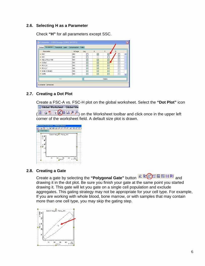
2.6. Selecting H as a Parameter

Check “H” for all parameters except SSC.

2.7. Creating a Dot Plot

Create a FSC-A vs. FSC-H plot on the global worksheet. Select the “Dot Plot” icon

( ) on the Worksheet toolbar and click once in the upper left corner of the worksheet field. A default size plot is drawn.

2.8. Creating a Gate

Create a gate by selecting the “Polygonal Gate” button and drawing it in the dot plot. Be sure you finish your gate at the same point you started drawing it. This gate will let you gate on a single cell population and exclude aggregates. This gating strategy may not be appropriate for your cell type. For example, If you are working with whole blood, bone marrow, or with samples that may contain more than one cell type, you may skip the gating step.

7

2.9. Selecting Parameters for Dot Plot Axes

Create another dot plot next to the FSC-A vs. FSC-H dot plot. This time, make it FSC-A vs. SSC-A. Change the parameters on your dot plot by left clicking on them and selecting the one you need in the pop-up menu.

To gate it on the P1 gate, right click inside the FSC-A vs. SSC-A dot plot and in the pop-up menu select “Show Populations”, then “P1”.

2.10. Creating an FSC-A vs. SSC-A Dot Plot

Create a gate on the FSC-A vs. SSC-A dot plot. Later you can adjust it to fit your population precisely.

8

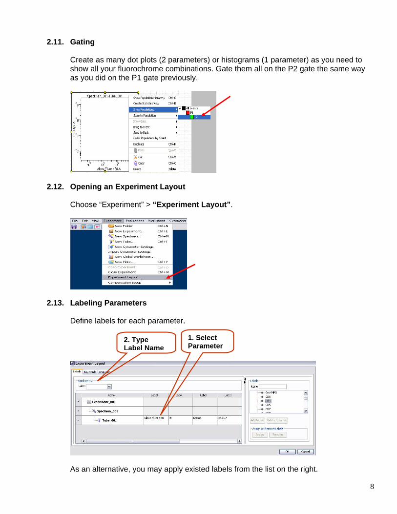
2.11. Gating

Create as many dot plots (2 parameters) or histograms (1 parameter) as you need to show all your fluorochrome combinations. Gate them all on the P2 gate the same way as you did on the P1 gate previously.

2.12. Opening an Experiment Layout

Choose “Experiment” > “Experiment Layout”.

2.13. Labeling Parameters

Define labels for each parameter.

As an alternative, you may apply existed labels from the list on the right.

1. Select Parameter

2. Type Label Name

9

2.14. Setting Up the Number of Events to Record

In the “Experiment Layout” dialog box, click the “Acquisition” tab. Here you can set the amount of events to record for each tube. If you don’t have specific preferences, we recommend that you record the same number of events in every tube. Select all tubes by clicking on the selecting dots located to the far left of your tube names while holding Shift. Then specify the number of events by using the “Events to Record” scroll down menu.

After that, select Global Worksheet.

Then, select Stopping Gate.

Leave “Storage Gate” value equal to “All Events”

After everything is set, click the “OK” button in the right lower corner of the “Experiment Layout” window.

10

2.15. Checking Laser Delay Parameters

In the Cytometer window, navigate to the “Laser” tab. Check the laser delay for the Red and Violet/UV lasers in the “Delay” column. It should be the same as on the printout that is located in front of the monitor.

2.16. Setting Up Voltages Based on an Unstained/Negative Control

Now you are ready to acquire your first tube. Your first tube should be an unstained and untreated control. Make sure that the pointer on the far left from the tube name is activated.

Place the tube on the Sample Injection Port (SIP). Press the “Low” and the “Run” buttons on the LSRII instrument. Click the “Acquire Data” button on the “Acquisition Dashboard”.

Adjust Voltages so you can see the population of interest in the center of the FSC-A vs. SSC-A dot plot. Adjust the voltages so the autofluorescent signals on each parameter form peaks within the first decade. You need to be able to see both the ascending and descending slopes of each peak.

11

2.17. Adjusting Area Scaling for FSC

Check area scaling for forward scatter: go to the “Laser” tab in the “Cytometer” window and adjust the “FSC Area Scaling” value until the population of interest on the FSC-A/FSC-H dot plot is aligned along the diagonal of the square dot plot box:

Normal Decrease “FSC Area Increase “FSC Area Scaling” for optimal Scaling” for optimal settings settings

12

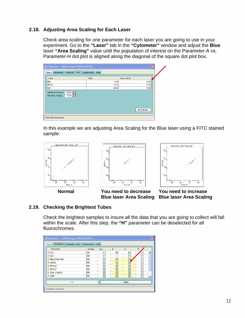
2.18. Adjusting Area Scaling for Each Laser

Check area scaling for one parameter for each laser you are going to use in your experiment. Go to the “Laser” tab in the “Cytometer” window and adjust the Blue laser “Area Scaling” value until the population of interest on the Parameter-A vs. Parameter-H dot plot is aligned along the diagonal of the square dot plot box.

In this example we are adjusting Area Scaling for the Blue laser using a FITC stained sample:

Normal You need to decrease You need to increase Blue laser Area Scaling Blue laser Area Scaling 2.19. Checking the Brightest Tubes

Check the brightest samples to insure all the data that you are going to collect will fall within the scale. After this step, the “H” parameter can be deselected for all fluorochromes.

13

3. Acquiring Compensation Controls and Calculating Compensation 3.1. Creating a Compensation Control Specimen

Create Compensation Controls if you are going to use more than one fluorochrome. Select “Compensation Setup” from the “Experiment” menu; then select “Create Compensation Controls”.

Each fluorophore is associated with one or several labels. For the majority of applications you can use the default label, “Generic”, and delete the rest of the entries. If within the experiment you are using different labels for the same fluorochromes and you have corresponding compensation controls for them, then you may choose to create additional compensation control tubes. Use the “Add” and “Delete” buttons to modify your preferences. Click the “OK” button to proceed.

3.2. Recording Compensation Tube Data

“Global Worksheet” should change to “Normal Worksheet” automatically. Click once on the plus sign (+) next to the Compensation Controls Specimen to expand it. Select “Unstained Control” by clicking on the icon to the left of the tube name. Place the tube with the unstained sample on the Sample Injection Port (SIP). Press the “Low” and the “Run” buttons on the LSRII instrument. Click the “Acquire Data” button, wait a few seconds until the threshold rate is stable, and then click the “Record Data” button on the Acquisition Dashboard. After you are done recording, adjust the P1 gate to include your population of interest. Then you may right click on the P1 gate and select “Apply to All Compensation Controls”. Record data for all tubes in the Compensation Control Specimen. Adjust P1 and P2 gates as needed.

14

3.3. Calculating Compensation

Navigate to “Experiment”, then “Compensation Setup”, and then select “Calculate Compensation”.

The computer will calculate compensation for all parameters. In the window that appears, select “Link & Save”

Switch back to Global Worksheet by clicking on the top left icon. Now you are ready to collect data for your samples.

The pointer on the far left of the tube for which you are about to record the data should be selected.

15

4. Exporting Recorded Data

After you finish recording your last sample, export your Experiment and FCS files. Right click on the name of your experiment and in the menu select “Export”, then “Experiments”.

In the window that appears, click the “Browse” button, then select “Desktop” as the destination folder and click “Export” to save your files there.

16

You also need to save the FCS files for analysis with third party software. Right click on the Experiment name again, select Export, but this time select FCS files to export.

Make sure you are exporting “FCS 2.0 files”; then press “OK”.

In the next window, click “Browse” to specify the directory path for the files you are exporting. We recommend saving them on the Desktop first or in the same folder as the Experiment.

5. Batch Analysis

Now you may choose to perform a batch analysis. It will give you the option to print multiple worksheets or save them as a PDF file. It will also allow you to export the data from the “Statistics View” to a CSV file that can be read in Excel.

17

To start a batch analysis you need to right click on your Experiment name (or Specimen, or several selected tubes) and select Batch Analysis.

Then select the actions you want the software to perform. Also, it is important to specify the destination where your PDF and CSV files are going to be saved. Click the “Browse” button and select the same folder as the experiment on the desktop in both cases. Copy your folders to a storage device and proceed with the cleaning procedure.

6. Logging Out from the Software

To log out from the software, select “Log Out” from the File menu.