BD FACSDiva Software Quick Start Guide

http://www.bdbioscienPart No. 338574 Rev. ASeptember 2004

BD Biosciences2350 Qume DriveSan Jose, CA 95131-1807USATel (877) 232-8995Fax (408) 954-2347

Asia Pacific

Fax (65) 6-860-1590Tel (65) 6-861-0633

IVD For In Vitro D

QuickStart.book Page i Monday, August 2, 2004 1:51 PM

BD FACSDivaSoftware

Quick Start Guide

ces.com/

MexicoTel (52) 55-5999-8296Fax (52) 55-5999-8288

JapanNippon Becton Dickinson

Tel 0120-8555-90

CanadaTel (888) 259-0187

Fax (905) 542-9391(905) 542-8028

[email protected]

Brazil Tel (55) 11-5185-9995/9941Fax (55) 11-5185-9895

BENEX LimitedBay K 1 a/dShannon Industrial EstateShannon, County Clare

Tel (353) 61-472920Fax (353) 61-472546

Ireland

Company, Ltd.

Europe Tel (32) 53-720211Fax (32) 53-720450

REPEC

iagnostic Use

QuickStart.book Page ii Monday, August 2, 2004 1:51 PM

© 2004, Becton, Dickinson and Company. All rights reserved. No part of this publication may be reproduced, transmitted, transcribed, stored in retrieval systems, or translated into any language or computer language, in any form or by any means: electronic, mechanical, magnetic, optical, chemical, manual, or otherwise, without prior written permission from BD Biosciences.

The information in this guide is subject to change without notice. BD Biosciences reserves the right to change its products and services at any time to incorporate the latest technological developments. Although this guide has been prepared with every precaution to ensure accuracy, BD Biosciences assumes no liability for any errors or omissions, nor for any damages resulting from the application or use of this information. BD Biosciences welcomes customer input on corrections and suggestions for improvement.

BD FACSDiva software © 2004, Becton, Dickinson and Company. This software is the property of Becton, Dickinson and Company. Each sale of a stored unit of this software grants the purchaser a nontransferable, nonexclusive, personal license. This software may not be duplicated, reproduced, or copied in any form or by any means whatsoever, except as otherwise permitted by law.

BD, the BD logo, and BD FACSDiva are trademarks of Becton, Dickinson and Company.

Microsoft and Windows are registered trademarks of Microsoft Corporation. All other company and product names may be trademarks of the respective companies with which they are associated.

PerCP is licensed under US Patent No. 4,876,190; Cy5.5 is licensed under US Patent Nos. 5,268,486; 5,486,616; 5,569,587; 5,569,766; and 5,627,027; APC and PE are licensed under US Patent Nos. 4,520,110; 4,859,582; 5,055,556; European Patent No. 76,695; Canadian Patent No. 1,179,942.

BD FACSDiva software is for in vitro diagnostic (IVD) use when used with IVD reagents and instruments. Refer to the information supplied by the manufacturer for application-specific limitations.

History

Revision Date Change Made

337647 Rev A 01/04 Initial release for BD FACSDiva software version 4.0.

338007 Rev A 04/04 Updated for version 4.0.1: CE IVD release

338574 09/04 Updated for software version 4.1; see the New Features section for details.

Modified: Creating an Experiment, Working With Experiments in the Browser, Importing Data, Using Tethering and Batch Analysis, Gating Multicolor Experiments, Setting Up Compensation Controls. New: Changing Browser Button Defaults, Using Biexponential Display.

QuickStart.book Page iii Monday, August 2, 2004 1:51 PM

Contents

About This Guide 5

New Features . . . . . . . . . . . . . . . . . . . . . . . . . . . . . . . . . . . . . . . . . . . . . . . . 5

Conventions . . . . . . . . . . . . . . . . . . . . . . . . . . . . . . . . . . . . . . . . . . . . . . . . . 8

Technical Assistance . . . . . . . . . . . . . . . . . . . . . . . . . . . . . . . . . . . . . . . . . . . 9

Getting Started 11

Becoming Familiar with the Workspace . . . . . . . . . . . . . . . . . . . . . . . . . . . . 12

Using Administrative Options . . . . . . . . . . . . . . . . . . . . . . . . . . . . . . . . . . . . 16

Adding a Password . . . . . . . . . . . . . . . . . . . . . . . . . . . . . . . . . . . . . . . . . 16

Creating a New User . . . . . . . . . . . . . . . . . . . . . . . . . . . . . . . . . . . . . . . 17

Sharing Experiments . . . . . . . . . . . . . . . . . . . . . . . . . . . . . . . . . . . . . . . 20

Viewing User-Specific Changes . . . . . . . . . . . . . . . . . . . . . . . . . . . . . . . . 21

Disabling a User . . . . . . . . . . . . . . . . . . . . . . . . . . . . . . . . . . . . . . . . . . . 23

Creating and Working with Experiments . . . . . . . . . . . . . . . . . . . . . . . . . . . 24

Creating a Folder and an Experiment . . . . . . . . . . . . . . . . . . . . . . . . . . . 24

Exporting an Experiment as a Template . . . . . . . . . . . . . . . . . . . . . . . . . 29

Creating an Experiment from a Template . . . . . . . . . . . . . . . . . . . . . . . 31

Importing an Experiment . . . . . . . . . . . . . . . . . . . . . . . . . . . . . . . . . . . . 32

Working with Experiments in the Browser . . . . . . . . . . . . . . . . . . . . . . . 33

Changing Browser Button Defaults . . . . . . . . . . . . . . . . . . . . . . . . . . . . 36

Using Gating Features . . . . . . . . . . . . . . . . . . . . . . . . . . . . . . . . . . . . . . . . . . 38

Creating Gates . . . . . . . . . . . . . . . . . . . . . . . . . . . . . . . . . . . . . . . . . . . . 38

Editing Gates . . . . . . . . . . . . . . . . . . . . . . . . . . . . . . . . . . . . . . . . . . . . . 40

Subsetting Populations . . . . . . . . . . . . . . . . . . . . . . . . . . . . . . . . . . . . . . 41

iii

QuickStart.book Page iv Monday, August 2, 2004 1:51 PM

Using Tethering, Batch Analysis, and Biexponential Display . . . . . . . . . . 48

Gating Multicolor Experiments . . . . . . . . . . . . . . . . . . . . . . . . . . . . . . . 55

Calculating Compensation Using Instrument Setup . . . . . . . . . . . . . . . . . . . . 63

Setting Up Compensation Controls . . . . . . . . . . . . . . . . . . . . . . . . . . . . . 63

Creating an Instrument Configuration . . . . . . . . . . . . . . . . . . . . . . . . . . 65

Importing Data and Calculating Compensation . . . . . . . . . . . . . . . . . . . 67

Calculating Compensation Manually . . . . . . . . . . . . . . . . . . . . . . . . . . . . . . 70

Adjusting FITC Compensation . . . . . . . . . . . . . . . . . . . . . . . . . . . . . . . . 70

Adjusting Compensation for the Remaining Tubes . . . . . . . . . . . . . . . . . 74

Manually Constructing a Compensation Matrix . . . . . . . . . . . . . . . . . . . 75

Maintaining the Database . . . . . . . . . . . . . . . . . . . . . . . . . . . . . . . . . . . . . . . 77

iv BD FACSDiva Software Quick Start Guide

QuickStart.book Page 5 Monday, August 2, 2004 1:51 PM

About This Guide

The BD FACSDiva Software Quick Start Guide contains tutorials designed to familiarize you with BD FACSDiva™ software. If you are a new user, use the tutorials to get started with the software. If you are an experienced user, try the updated tutorials to become familiar with new software features. Updated tutorials are highlighted in the New Features section.

New Features

This version of BD FACSDiva software includes support for plate-based acquisition using the BD™ High Throughput Sampler on the BD™ LSR II flow cytometer.

New features that are available to all instruments include the following.

Workspace Features

• The New Experiment button now creates an Experiment with no Specimen or Tube. However, you can customize the button to create any Experiment template. The New Specimen, New Tube, and New Global Worksheet buttons can be customized as well. For information, see Template Preferences in the BD FACSDiva Software Reference Manual. To practice using this and other workspace features, go to Creating a Folder and an Experiment on page 24 and Changing Browser Button Defaults on page 36.

• The Browser search buttons are now represented by icons. To view a button’s function, place your mouse cursor over the button.

• The acquisition pointer is no longer set automatically. You choose where to set the pointer when you start a new Experiment, or open an existing one.

5


Analysis Features

• Biexponential scaling can be used to show all events on plots, even those with negative values that fall on-axis when shown on a log plot. Additionally, during a batch analysis, you can elect to process all Tubes with different biexponential scales. For information, see Using Biexponential Scaling in the BD FACSDiva Software Reference Manual; for a tutorial highlighting this feature, see Using Tethering, Batch Analysis, and Biexponential Display on page 48 of this guide.

• Quadrant gate segments can now be offset or rotated on a pivot point. These features are highlighted in the tutorial on Gating Multicolor Experiments on page 55. For general information, see Drawing Manual Gates in the BD FACSDiva Software Reference Manual.

• Contour plots can now be formatted as Density plots. For information, see Formatting Density Plots in the BD FACSDiva Software Reference Manual.

• By default, the plot background color is now set to white. A new user preference allows you to change the background color, and choose whether to always print black plots with a white background. See Plot Preferences in the BD FACSDiva Software Reference Manual. Note that plots with a colored background are now printed in the specified color.

• Snap-To Interval gates can now be tethered to manual gates. In addition, the Auto-Size and Auto-Movement features can now be used with Snap-To Interval gates. For more information, see Working With Snap-To Gates in the BD FACSDiva Software Reference Manual.

Acquisition Features

• The way you work with instrument settings has been simplified in this version. When the software is connected to the cytometer, you can now edit settings only for the current acquisition Tube in the Instrument frame; the Inspector shows an instrument settings report for a selected object. This feature is highlighted in Working with Experiments in the Browser on page 33. During offline use, settings can be edited in the Inspector.

Additionally, the Experiment Inspector contains a new control which allows you to apply instrument setting changes at the Tube or Specimen

6 BD FACSDiva Software Quick Start Guide


level to the global (Experiment-level) settings. When this preference is enabled, global settings are updated to reflect changes to Tube- and Specimen-specific settings, and the new global settings automatically apply to the remaining unrecorded Tubes and Specimens in the Experiment. For more information, see Using Global Instrument Settings in the BD FACSDiva Software Reference Manual.

• Instrument Setup controls are now managed through a dialog box, where you can specify parameters and define label-specific controls. For a demonstration of this feature, try the tutorial on Calculating Compensation Using Instrument Setup on page 63. For general information, see Creating Compensation Controls in the BD FACSDiva Software Reference Manual.

• Default templates are now provided for certain instrument functions, such as daily instrument quality control or routine sorting experiments. For details, refer to the updated instrument manual or instrument online help provided with this software release.

• Area scaling can now be adjusted for the FSC parameter on all instruments. For information, see Using Area Scaling in the BD FACSDiva Software Reference Manual. To see if FSC area scaling should be verified during daily quality control for your instrument, refer to the updated instrument manual or instrument online help provided with this software release.

• A time-stopping rule has been implemented for the BD FACS™ Loader on the BD FACSCanto™ flow cytometer. The time is set on the Carousel Controls frame. For more information, refer to the updated BD FACS Loader User’s Guide or instrument online help provided with this software release.

Other Features and Changes

Other improvements in this version include:

• quicker menu responsiveness

• a disk check to verify storage space before recording

• no flickering or scrolling of the Browser

• lin/log display settings saved with FCS files

About This Guide 7


• population names shown in drill-down plot headers

• user login names sorted alphabetically

• Time plot display buffer preserved each time new events are added

• keyword values and suffixes retained when a recorded Tube is copied/pasted or when an Experiment template is exported

• Experiment and Specimen keywords saved with Tubes

• tape backup and FTP export functions removed

• statistics appended to exported .csv file during batch analysis

Conventions

The following table lists conventions used in this guide.

Table 1 Text and keyboard conventions

Convention Use

Tip Highlights features or hints that can save time and prevent difficulties

NOTICE Describes important features or instructions

> The arrow indicates a menu choice. For example, “choose File > Print” means to choose Print from the File menu.

Ctrl-XWhen used with key names, a dash means to press two keys simultaneously. For example, Ctrl-P means to hold down the Control key while pressing the letter p.



Technical Assistance

For technical questions or assistance in solving a problem:

• In BD FACSDiva software, choose Help > Online Help. Locate and read topics specific to the operation you are performing.

To quickly find information on any topic, enter search terms on the Search tab. You can search individual books, or search all books at once. You can also use the Contents or Index tab to find information. To find software information, click to expand topics in the Software Help book; to find instrument information, expand the Instrument Help book.

• Refer to the Troubleshooting section in the Software or Instrument Help books.

If additional assistance is required, contact your local BD Biosciences technical support representative or supplier.

When contacting BD Biosciences, have the following information available:

• product name, part number, and serial number; software version and computer system specifications

• any error messages

• details of recent instrument performance

For instrument support from within the US, call (877) 232-8995, prompt 2, 2.

For support from within Canada, call (888) 259-0187.

Customers outside the US and Canada, contact your local BD representative or distributor.

About This Guide 9




Getting Started

Use the following tutorials to learn how to use BD FACSDiva™ software if you are a new user, or practice using new features if you are an experienced user.

• Becoming Familiar with the Workspace on page 12

• Using Administrative Options on page 16

• Creating and Working with Experiments on page 24

• Using Gating Features on page 38

• Calculating Compensation Using Instrument Setup on page 63

• Calculating Compensation Manually on page 70

• Maintaining the Database on page 77

11


Before You Begin

• If you already have BD FACSDiva software on your system, upgrade it using the instructions provided with the installation CD. After the upgrade, restart your instrument and computer as described in the upgrade instructions.

• If you are new to BD FACSDiva software, start the software by double-clicking the shortcut icon on the desktop.

When the Log In dialog box appears, click OK. Note that no password is required the first time you log into the software. For more information about user login, see Using Administrative Options on page 16.

Becoming Familiar with the Workspace

After a successful login, frames containing the main application components are displayed in the BD FACSDiva workspace (Figure 1 on page 13). You can hide or show frames by clicking buttons in the Workspace toolbar ( in the figure).

If you are new to BD FACSDiva software, take a minute to become familiar with the main frames. Note that some software features are instrument-specific, so your workspace might look different from that shown in this example. For information about instrument-specific software components, refer to your instrument manual.

shortcut icon

1



Figure 1 BD FACSDiva workspace

Click a button in the Workspace toolbar to hide or show the corresponding frame. Frames can be resized by dragging a border or corner.

The Browser frame lists folders, Experiments, and experimental elements in a hierarchical view, provides an interface for setting up Experiments, and contains a Current Tube pointer (c) indicating the Tube for which acquisition or analysis data will be shown.

Only one Experiment can be open at a time. In an open Experiment, you can add, rename, or copy elements, and record or display data.

Click a button in the Browser toolbar (a) to add elements to the Browser. To display fewer Experiments, enter a term in the search field (b) and click the Find button (d).

1

24

5

6

73

1

2

a

c

b

d

Becoming Familiar with the Workspace 13


The Acquisition Controls frame contains controls for acquiring and recording data.

The Instrument frame shows instrument connectivity status. When you are connected to an instrument, the frame also shows status messages and laser controls. If an Experiment is open and the Current Tube pointer is set, the frame displays instrument settings for the current acquisition Tube.

Additional controls might be displayed in this frame depending on the instrument you are running; refer to your instrument manual for a description.

Use the Inspector frame to view or modify the attributes of one or more objects in the worksheet or Browser frames. The contents of the Inspector change depending on what is selected.

3

4

5



The Worksheet frame is where you create global or normal worksheets containing plots, gates, statistics, and custom text. Global worksheets have green-tinted tabs, while normal worksheets have gray-tinted tabs (a).

Click a button in the Worksheet toolbar (b) to switch between the global or normal worksheets view, create analysis objects or free text, or align objects on a worksheet.

The Acquisition Status frame gives ongoing status during acquisition or recording.

6

b

a

7

Becoming Familiar with the Workspace 15


Using Administrative Options

If you have administrator privileges, BD FACSDiva software allows you to create additional user names which can be password-protected. Experiments, workspace setup, and user preferences are saved with your login name. After login, other users cannot view your Experiments unless they have administrative access, or you have designated an Experiment as shared.

The following tutorials describe how to create a new user, and show how workspace setup, user preferences, and the Browser view differ from one user to another.

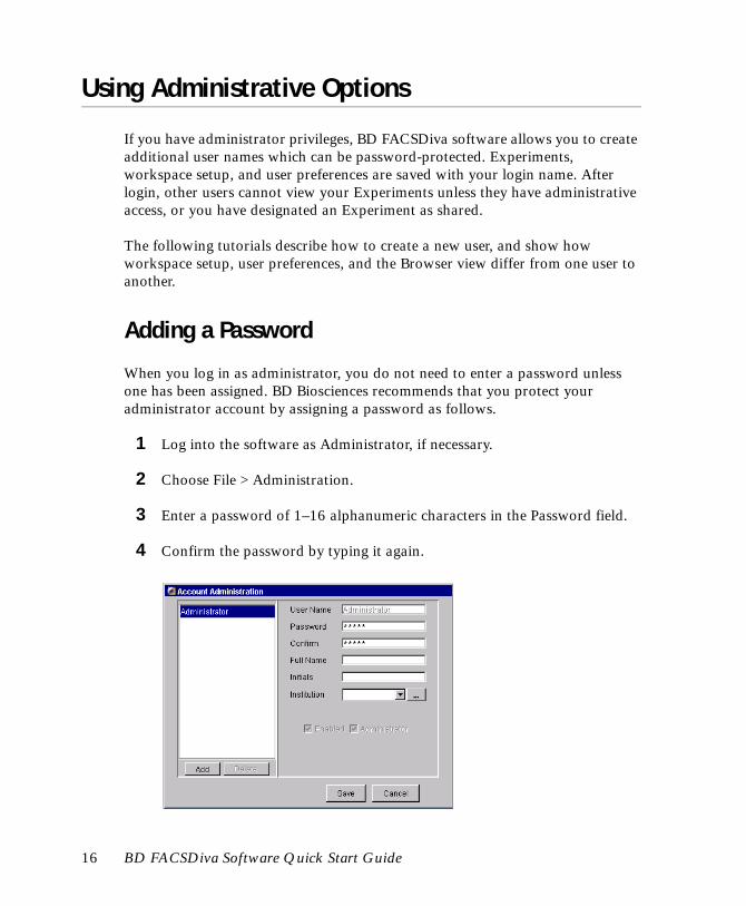
Adding a Password

When you log in as administrator, you do not need to enter a password unless one has been assigned. BD Biosciences recommends that you protect your administrator account by assigning a password as follows.

1 Log into the software as Administrator, if necessary.

2 Choose File > Administration.

3 Enter a password of 1–16 alphanumeric characters in the Password field.

4 Confirm the password by typing it again.



5 Enter your name, initials, and institution if you would like.

For instructions on adding institution names to the drop-down menu, see steps 8 through 10 under Creating a New User.

6 Click Save.

Tip Keep a copy of your password in a secure location in case you forget it.

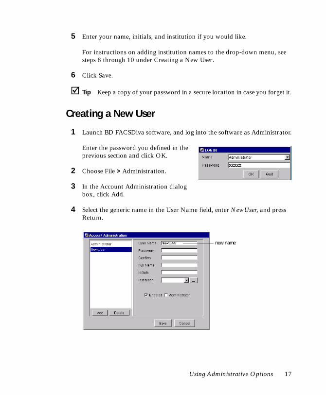
Creating a New User

1 Launch BD FACSDiva software, and log into the software as Administrator.

Enter the password you defined in the previous section and click OK.


3 In the Account Administration dialog box, click Add.

4 Select the generic name in the User Name field, enter NewUser, and press Return.

new name

Using Administrative Options 17


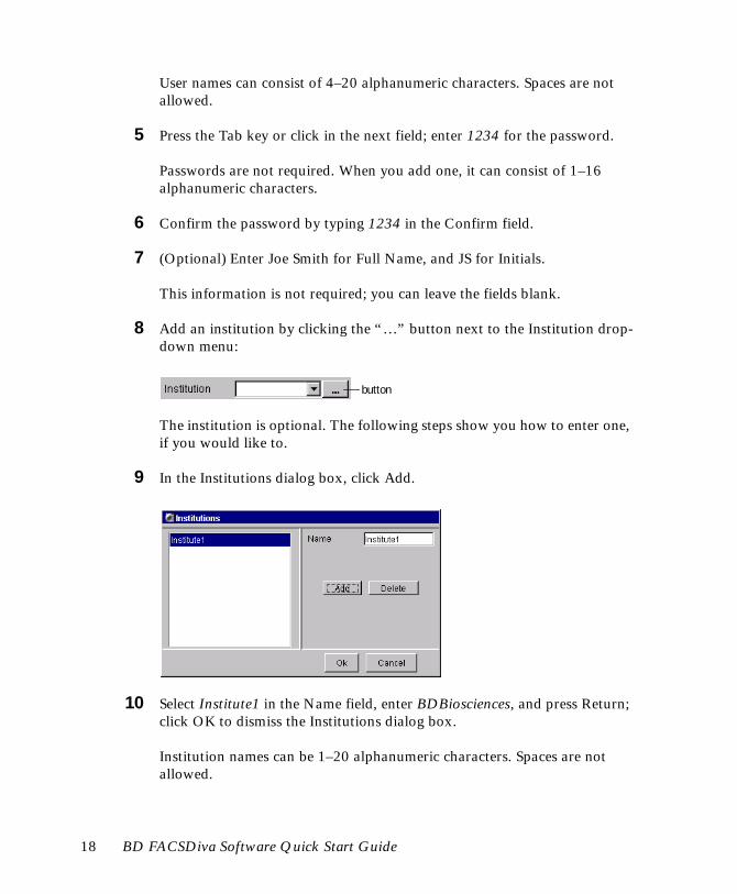
User names can consist of 4–20 alphanumeric characters. Spaces are not allowed.

5 Press the Tab key or click in the next field; enter 1234 for the password.

Passwords are not required. When you add one, it can consist of 1–16 alphanumeric characters.

6 Confirm the password by typing 1234 in the Confirm field.

7 (Optional) Enter Joe Smith for Full Name, and JS for Initials.

This information is not required; you can leave the fields blank.

8 Add an institution by clicking the “…” button next to the Institution drop-down menu:

The institution is optional. The following steps show you how to enter one, if you would like to.

9 In the Institutions dialog box, click Add.

10 Select Institute1 in the Name field, enter BDBiosciences, and press Return; click OK to dismiss the Institutions dialog box.

Institution names can be 1–20 alphanumeric characters. Spaces are not allowed.

button



11 Choose BDBiosciences from the Institution drop-down menu in the Account Administration dialog box.

12 Leave the Enabled checkbox selected, and the Administrator checkbox deselected.

Deselect the Enabled checkbox only when you want to disable a user. For more information, see Disabling a User on page 23.

Select the Administrator checkbox only when you want to give one of your users privileges to create and disable users, or view all users’ Experiments.

13 Click Save to add the new user.

NewUser will be available as a login name the next time you log into the software, as you will see in the next tutorial.



Sharing Experiments

When you log into BD FACSDiva software, all your saved Experiments are listed under your user icon in the Browser. Other users will not be able to view your Experiments unless they have administrative access, or you have designated an Experiment as shared.

The following steps demonstrate how to share an Experiment, and show how the Browser view changes when you log in as another user.

1 Right-click any Experiment in the Browser and choose Share Experiment.

If you have not yet created any Experiments, click the New Experiment button ( ) twice to create two new Experiments. Designate only one of the new Experiments as shared.

The Experiment icon changes to show that the Experiment is shared.

2 Choose File > Log Out to log out as Administrator.

3 Log back into the software as NewUser.

Remember to enter 1234 as the password.

When the workspace appears, notice that the user icon in the Browser now reads NewUser.

4 Click the plus sign (+) next to the Shared View icon in the Browser.

The Experiment you shared can be accessed under the Shared View icon.

shared icon



5 Open the shared Experiment by double-clicking it.

6 Change the Experiment by adding or deleting a Tube.

To add a Tube, click the New Specimen or New Tube button in the Browser toolbar. To delete one, right-click any Tube and choose Delete.

Any changes you make to a shared Experiment can be viewed by all other users. You will see your changes when you log back in as Administrator in the next section.

Viewing User-Specific Changes

Along with Experiments, workspace setup and user preferences are saved with your login name. Before you log out as NewUser, change the user preferences and the workspace. You will see that these changes are saved when you log back in.

1 Choose Edit > User Preferences.

2 Click the Gates tab and change the default preferences to the following:

Click OK to dismiss the User Preferences dialog box.

3 Click buttons in the Workspace toolbar to hide all frames but the Browser.



4 Resize the BD FACSDiva window so it is half the width it is now.

5 Choose File > Log Out.

6 Log into the software as Administrator.

As the instrument connects, notice that the window changes to the size it was previously, and that the four main workspace frames are now shown.

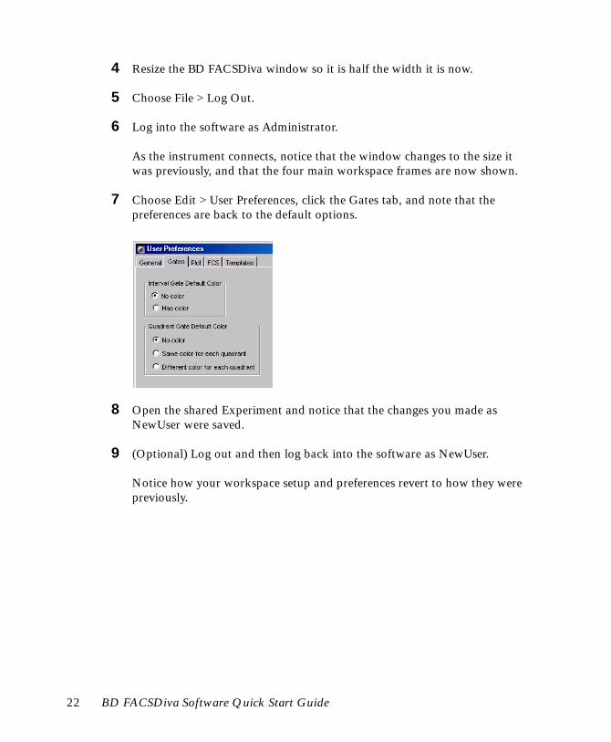
7 Choose Edit > User Preferences, click the Gates tab, and note that the preferences are back to the default options.

8 Open the shared Experiment and notice that the changes you made as NewUser were saved.

9 (Optional) Log out and then log back into the software as NewUser.

Notice how your workspace setup and preferences revert to how they were previously.



Disabling a User

Once a user has saved Experiments in the database, you cannot delete their user name from the list, but you can disable them. A disabled user can no longer log into the application. However, their Experiments are saved in the database and their shared Experiments are available to all users.

Only Administrators or those with administrative access can delete or disable other users.

1 Log into the software as Administrator, if necessary.


3 Select NewUser in the list of users, and deselect the Enabled checkbox.

4 Click Save to save your changes and dismiss the dialog box.

5 (Optional) Log out and then back into the software and verify that NewUser is not available as a login name.



Creating and Working with Experiments

An Experiment is a group of elements used to acquire and analyze data from the flow cytometer. You build Experiments as you acquire and analyze data. The Browser is where you create Experiments and access stored data.

There are three ways to add Experiments to the Browser.

• Use the New Experiment button ( ) in the Browser toolbar to create a new, empty Experiment with default instrument settings. Note that the button can be customized to add any Experiment template, as you will see in Changing Browser Button Defaults on page 36.

• Use the Experiment > New Experiment command to create a new Experiment based on a saved template with customized elements such as plots, gates, statistics views, and instrument settings.

• Use the File > Import > Experiments command to access Experimental elements and data from an archived Experiment.

The following tutorials describe how to use each of these commands and how to work with the resulting Experiments in the Browser. Note that you must be connected to the instrument to use some of the features in this section. If needed, start up your instrument and launch and log into the software before you begin the procedures in this section.

Creating a Folder and an Experiment

This section describes how to create a practice folder and an Experiment containing basic analysis options.

1 Click the New Folder button ( ) in the Browser toolbar.

2 Rename the folder Practice.

To rename any Browser object, select it in the Browser and start typing. Press Enter to apply the new name.

new folder



Notice that the folder is placed at the top of the Browser list. Folders are listed in the Browser in the order they are created.

3 Select the Practice folder and click the New Experiment button in the Browser toolbar.

Tip To place an Experiment in a folder, you need to select the folder before you create the Experiment.

A new, open Experiment is added below the folder in the Browser. The Experiment contains default instrument settings and a global worksheet. The Worksheet frame shows a blank global worksheet (indicated by a green-tinted tab).

4 Click the New Specimen button to add a Specimen and Tube to the Experiment.

Tip Click once on the plus sign (+) next to the Specimen to view the Tube.

5 Click to set the Current Tube pointer next to Tube_001 in the Browser.

The pointer changes to green, and four green-tinted tabs appear in the Instrument frame. The Current Tube pointer indicates the Tube for which instrument settings adjustments will apply and for which acquisition data will be shown.

If you are familiar with a previous version of BD FACSDiva software, notice that you have to click to set the pointer; the pointer is no longer automatically set when you open or start an Experiment.

pointer

Creating and Working with Experiments 25


6 Select each item in the Browser and notice how the Inspector changes.

When the Tube is selected, notice there are four tabs in the Inspector. Click each tab in turn to view the different Tube options.

In this version of the software, certain instrument settings can no longer be edited in the Inspector. When you are connected to the instrument, you can now change voltages, thresholds, and ratios only in the Instrument frame.

7 Choose Experiment > Experiment Layout, and define labels for each parameter.

Click in the FITC field and enter CD4; press the Tab key and enter CD16+56 for PE. Label the remaining fields with appropriate labels:

Tip When your Experiment contains many Tubes, you can use Experiment Layout to label all Tubes at once.

tabs



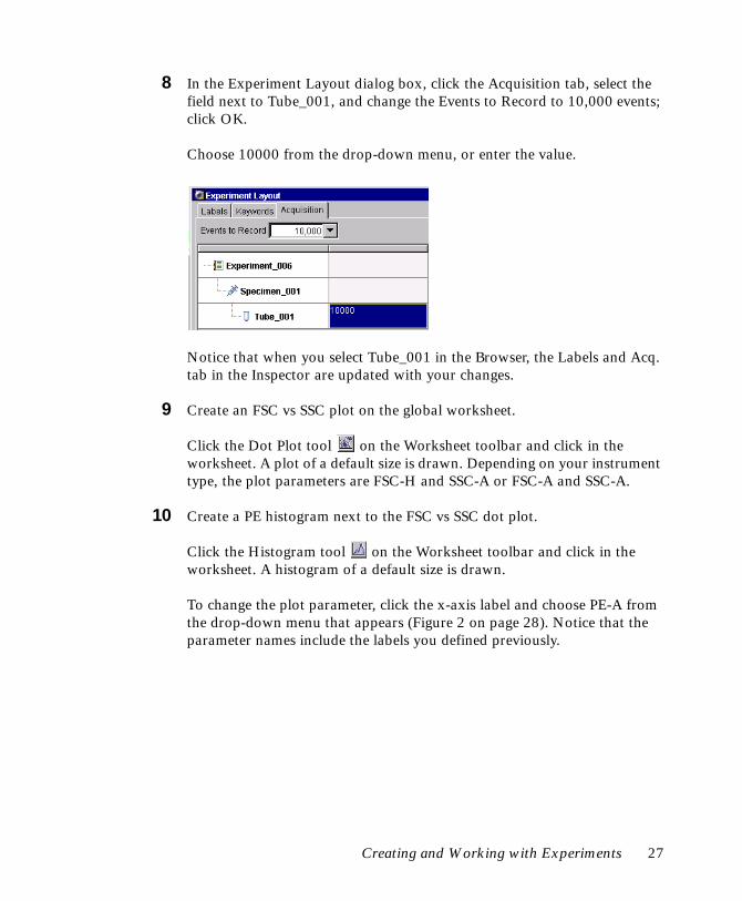
8 In the Experiment Layout dialog box, click the Acquisition tab, select the field next to Tube_001, and change the Events to Record to 10,000 events; click OK.

Choose 10000 from the drop-down menu, or enter the value.

Notice that when you select Tube_001 in the Browser, the Labels and Acq. tab in the Inspector are updated with your changes.

9 Create an FSC vs SSC plot on the global worksheet.

Click the Dot Plot tool on the Worksheet toolbar and click in the worksheet. A plot of a default size is drawn. Depending on your instrument type, the plot parameters are FSC-H and SSC-A or FSC-A and SSC-A.

10 Create a PE histogram next to the FSC vs SSC dot plot.

Click the Histogram tool on the Worksheet toolbar and click in the worksheet. A histogram of a default size is drawn.

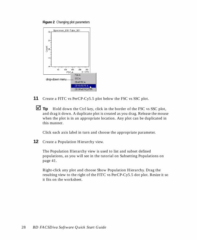
To change the plot parameter, click the x-axis label and choose PE-A from the drop-down menu that appears (Figure 2 on page 28). Notice that the parameter names include the labels you defined previously.



Figure 2 Changing plot parameters

11 Create a FITC vs PerCP-Cy5.5 plot below the FSC vs SSC plot.

Tip Hold down the Ctrl key, click in the border of the FSC vs SSC plot, and drag it down. A duplicate plot is created as you drag. Release the mouse when the plot is in an appropriate location. Any plot can be duplicated in this manner.

Click each axis label in turn and choose the appropriate parameter.

12 Create a Population Hierarchy view.

The Population Hierarchy view is used to list and subset defined populations, as you will see in the tutorial on Subsetting Populations on page 41.

Right-click any plot and choose Show Population Hierarchy. Drag the resulting view to the right of the FITC vs PerCP-Cy5.5 dot plot. Resize it so it fits on the worksheet.

drop-down menu



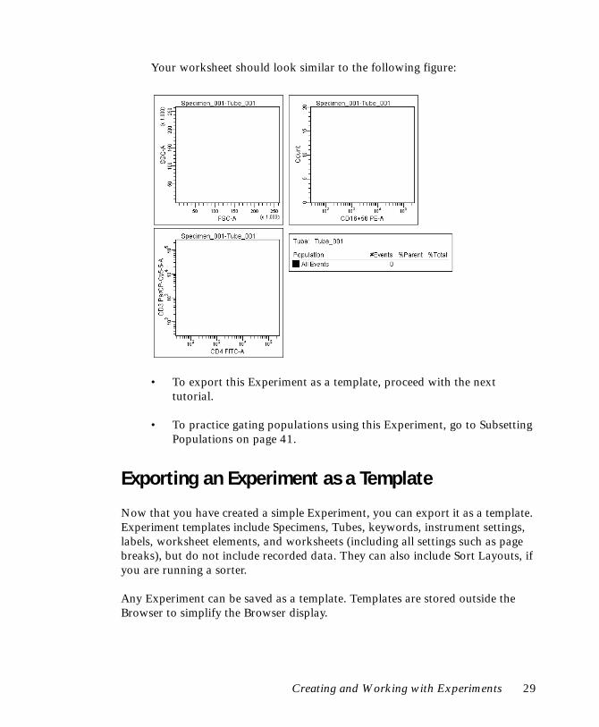
Your worksheet should look similar to the following figure:

• To export this Experiment as a template, proceed with the next tutorial.

• To practice gating populations using this Experiment, go to Subsetting Populations on page 41.

Exporting an Experiment as a Template

Now that you have created a simple Experiment, you can export it as a template. Experiment templates include Specimens, Tubes, keywords, instrument settings, labels, worksheet elements, and worksheets (including all settings such as page breaks), but do not include recorded data. They can also include Sort Layouts, if you are running a sorter.

Any Experiment can be saved as a template. Templates are stored outside the Browser to simplify the Browser display.



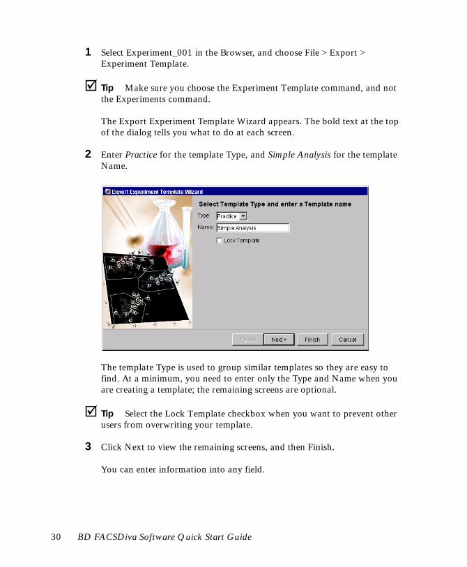
1 Select Experiment_001 in the Browser, and choose File > Export > Experiment Template.

Tip Make sure you choose the Experiment Template command, and not the Experiments command.

The Export Experiment Template Wizard appears. The bold text at the top of the dialog tells you what to do at each screen.

2 Enter Practice for the template Type, and Simple Analysis for the template Name.

The template Type is used to group similar templates so they are easy to find. At a minimum, you need to enter only the Type and Name when you are creating a template; the remaining screens are optional.

Tip Select the Lock Template checkbox when you want to prevent other users from overwriting your template.

3 Click Next to view the remaining screens, and then Finish.

You can enter information into any field.



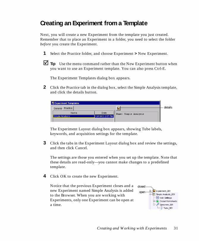
Creating an Experiment from a Template

Next, you will create a new Experiment from the template you just created. Remember that to place an Experiment in a folder, you need to select the folder before you create the Experiment.

1 Select the Practice folder, and choose Experiment > New Experiment.

Tip Use the menu command rather than the New Experiment button when you want to use an Experiment template. You can also press Ctrl-E.

The Experiment Templates dialog box appears.

2 Click the Practice tab in the dialog box, select the Simple Analysis template, and click the details button.

The Experiment Layout dialog box appears, showing Tube labels, keywords, and acquisition settings for the template.

3 Click the tabs in the Experiment Layout dialog box and review the settings, and then click Cancel.

The settings are those you entered when you set up the template. Note that these details are read-only—you cannot make changes to a predefined template.

4 Click OK to create the new Experiment.

Notice that the previous Experiment closes and a new Experiment named Simple Analysis is added to the Browser. When you are working with Experiments, only one Experiment can be open at a time.

details

closed

open



Notice that the global worksheet includes the plots and Population Hierarchy view you set up previously, and there is no data in the plots. When you start an Experiment from a template, analysis objects are included but the Experiment does not contain data.

Importing an Experiment

Next, you will import an Experiment into the Practice folder. Imported Experiments are different from templates in that they contain recorded data.

1 Select the Practice folder in the Browser, and choose File > Import > Experiments.

Remember that to place an Experiment in a folder, select the folder before you create the Experiment.

Tip If you forget to select the folder first, you can move an Experiment using Cut and Paste With Data commands.

By default, the D:\BDExport\Experiment folder appears when you import or export an Experiment, unless you previously navigated to a different folder.

2 Select the folder labeled Manual Comp, and click Import.

Experiments to import are always represented by a folder. The folder will be converted to an Experiment icon after it is imported into the Browser. To select the folder, click once (do not double-click), and then click Import.



Notice that the previous Experiment does not close. The new Experiment is added below the Simple Analysis Experiment in the Browser.

Working with Experiments in the Browser

You should now have three Experiments in the Browser: a closed default Experiment (Experiment_001), an open Experiment template (Simple Analysis), and a closed imported Experiment (Manual Comp).

The following exercise demonstrates the difference between closed and open Experiments, and shows how to use the frames to compare instrument settings.

1 Click once on the plus sign (+) next to the Manual Comp Experiment to expand it.

Although the Experiment’s contents are shown in the Browser, the plots are still blank. You must open an Experiment to access its stored data.

NOTICE Expanding an Experiment is not the same thing as opening it by double-clicking.

2 Double-click the Manual Comp Experiment to open it.

The Simple Analysis Experiment closes. Analysis objects for the Manual Comp Experiment are shown on the worksheet.

3 Click to expand one of the Experiment’s Specimens.

The Manual Comp Experiment contains multiple Tubes under each Specimen. Notice that each Tube icon has green highlighting, indicating that the Tube contains saved data.



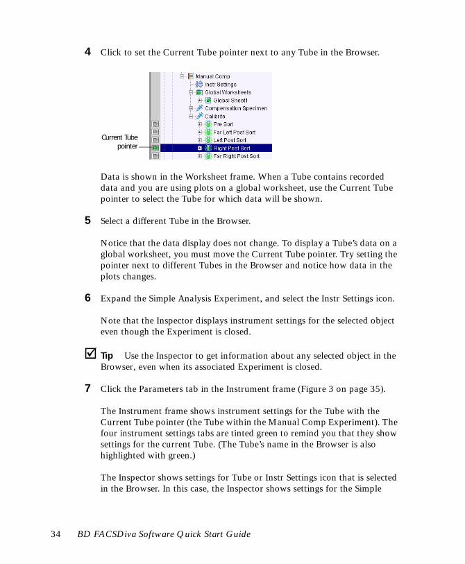
4 Click to set the Current Tube pointer next to any Tube in the Browser.

Data is shown in the Worksheet frame. When a Tube contains recorded data and you are using plots on a global worksheet, use the Current Tube pointer to select the Tube for which data will be shown.

5 Select a different Tube in the Browser.

Notice that the data display does not change. To display a Tube’s data on a global worksheet, you must move the Current Tube pointer. Try setting the pointer next to different Tubes in the Browser and notice how data in the plots changes.

6 Expand the Simple Analysis Experiment, and select the Instr Settings icon.

Note that the Inspector displays instrument settings for the selected object even though the Experiment is closed.

Tip Use the Inspector to get information about any selected object in the Browser, even when its associated Experiment is closed.

7 Click the Parameters tab in the Instrument frame (Figure 3 on page 35).

The Instrument frame shows instrument settings for the Tube with the Current Tube pointer (the Tube within the Manual Comp Experiment). The four instrument settings tabs are tinted green to remind you that they show settings for the current Tube. (The Tube’s name in the Browser is also highlighted with green.)

The Inspector shows settings for Tube or Instr Settings icon that is selected in the Browser. In this case, the Inspector shows settings for the Simple

Current Tubepointer



Analysis Experiment’s instrument settings. You can use the Instrument frame and Inspector to compare instrument settings for any two objects in the Browser.

Figure 3 Comparing instrument settings

8 In the Manual Comp Experiment, expand one of the Tubes under the Compensation Specimen and compare instrument settings to one of the Calibrite Tubes.

• Click to place the Current Tube pointer next to any Tube under the Compensation Specimen.

• Click the Parameters tab in the Instrument frame.

• Expand the Calibrite Specimen, if needed, and expand any Tube under the Specimen.

• Select the Instr Settings icon under the Tube. Settings are shown in the Inspector.

The settings should be the same.

9 Double-click the Manual Comp Experiment to close it.

settings forcurrent Tube

Inspector:settings for selectedInstr Settings icon

Instrument frame:



Changing Browser Button Defaults

You can assign any saved template to a button in the Browser toolbar. For example, Experiment templates can be assigned to the New Experiment button, panel templates can be assigned to the New Specimen button, and analysis templates can be assigned to the New Tube or New Global Worksheet button. The corresponding template is added to the Browser when you click the button in the Browser toolbar.

The following tutorial describes how to change template assignments for the Experiment button.

1 Choose Edit > User Preferences.

2 Click the Templates tab.

By default, the New Experiment button creates a blank Experiment.

3 Click the Templates button next to the Experiment field.

The Experiment Templates dialog box appears.



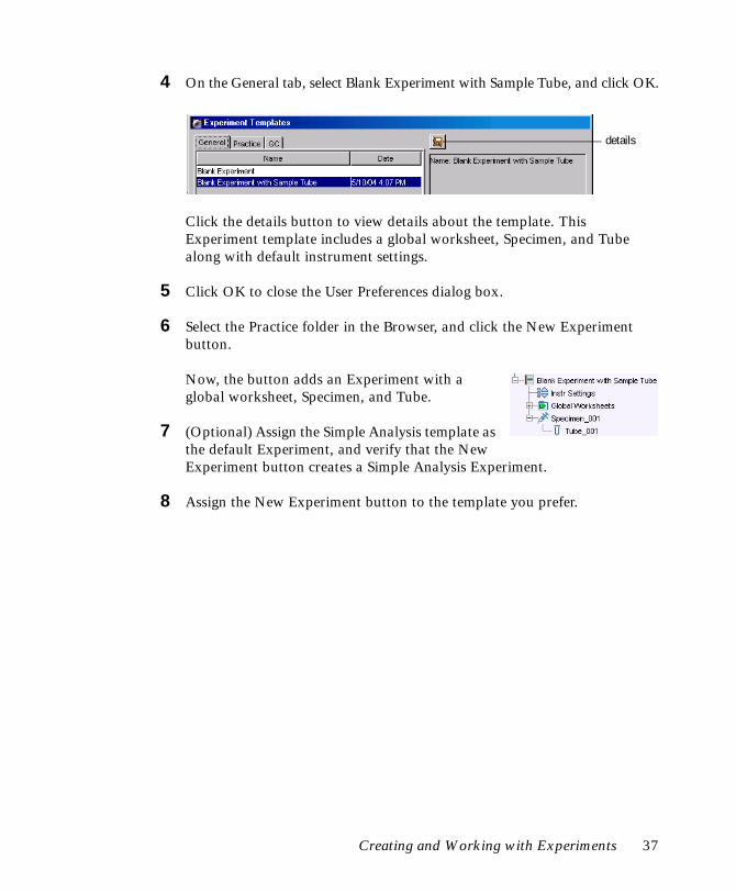
4 On the General tab, select Blank Experiment with Sample Tube, and click OK.

Click the details button to view details about the template. This Experiment template includes a global worksheet, Specimen, and Tube along with default instrument settings.

5 Click OK to close the User Preferences dialog box.

6 Select the Practice folder in the Browser, and click the New Experiment button.

Now, the button adds an Experiment with a global worksheet, Specimen, and Tube.

7 (Optional) Assign the Simple Analysis template as the default Experiment, and verify that the New Experiment button creates a Simple Analysis Experiment.

8 Assign the New Experiment button to the template you prefer.

details



Using Gating Features

You can create four types of gates in BD FACSDiva software: polygon, rectangle, quadrant, and interval. Automatic and Snap-To gating tools are available to create polygon and interval gates. The following exercises demonstrate the use of gating tools in BD FACSDiva software.

For this section, you will need both the Simple Analysis and Manual Comp Experiments from the previous section. If you are starting here, create the Simple Analysis Experiment as described in Creating a Folder and an Experiment on page 24, and import the Manual Comp Experiment as described in Importing an Experiment on page 32.

You do not need to be connected to the instrument to perform these exercises. If you are not connected, you will see a plot icon for the Current Tube pointer in the Browser rather than a pointer icon.

Creating Gates

This section describes how to use tools in the Worksheet toolbar to create different types of gates around populations in the Manual Comp Experiment.

1 Open the Manual Comp Experiment.

2 Set the Current Tube pointer to the Pre Sort Tube under the Calibrite Specimen.

The plots show data for that Tube.

3 Create an Autopolygon gate around the singlet events in the FSC vs SSC dot plot.



• Select the Autopolygon tool in the Worksheet toolbar ( ).

• Click the singlet events in the plot. A gate is drawn automatically.

4 Move the pointer to the next Tube in the Browser; notice that some of the events are outside the gate.

5 Select the Autopolygon gate in the FSC vs SSC plot, and press Delete.

Tip Press the Delete key, not the Backspace key. If the Delete key doesn’t work, right-click the gate and choose Delete. This will activate the Delete key for the next time you use it.

6 Create a Snap-To polygon gate ( ) around the singlet events in the FSC vs SSC dot plot.

Unlike an autopolygon gate, a Snap-To gate automatically recalculates as new data is provided to the gate. Notice that the gate boundary is thicker to differentiate the Snap-To feature.

7 Move the pointer back to the Pre Sort Tube and notice how the gate changes.

Using Gating Features 39


8 (Optional) To practice using the other gating tools, delete the Snap-To gate and create a Rectangle gate ( ) and then a Polygon gate ( ) around the singlet events in the plot.

To use the Polygon Gate tool, do the following:

• Select the Polygon tool in the Worksheet toolbar ( ).

• Move the cursor over the plot: it changes to a crosshair.

• Click to set the first vertex.

• Release the mouse button and move the cursor to where you want the second vertex and click again.

• Continue moving the cursor around the population and clicking until the population is completely encompassed by the gate.

• Close the region by double-clicking or by clicking on the first vertex.

For more practice creating gates, go to Subsetting Populations on page 41 and Gating Multicolor Experiments on page 55.

Editing Gates

This section describes how to move and resize gates.

1 Select the gate you created in the FSC vs SSC dot plot.

Handles appear at each vertex.



2 Drag the selected gate to move it.

To move a gate, select the gate border, not one of the vertices.

Notice that the gate label moves with the gate.

3 Drag one of the selection handles to resize the gate.

After you move or resize a Snap-To gate, the gate no longer adjusts automatically. You can force the gate to readjust by right-clicking on the gate boundary and choosing Recalculate from the contextual menu that appears.

4 Move the gate label by dragging it.

A gate label can be moved only when its gate is selected.

5 Click outside the plot boundary to deselect the gate.

6 Close the Manual Comp Experiment.

Subsetting Populations

The Simple Analysis Experiment you set up previously includes three plots and a Population Hierarchy view. The Population Hierarchy view is used to view defined populations and display the relationship between different gated populations. This section describes how to subset populations using the Population Hierarchy view.

For this tutorial, you will need the Simple Analysis Experiment that was created in Creating a Folder and an Experiment on page 24, and sample files that were installed in your BDExport\FCS folder during software installation.



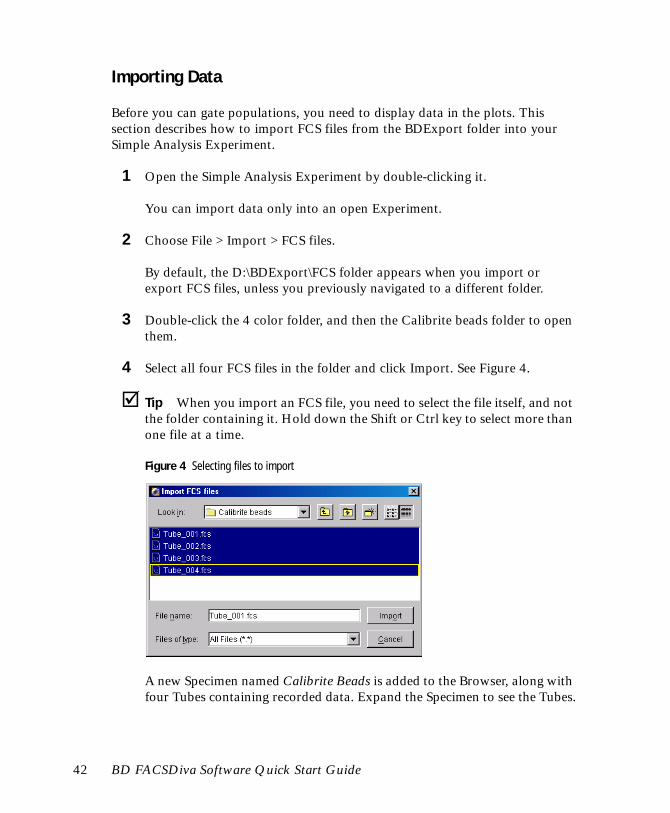
Importing Data

Before you can gate populations, you need to display data in the plots. This section describes how to import FCS files from the BDExport folder into your Simple Analysis Experiment.

1 Open the Simple Analysis Experiment by double-clicking it.

You can import data only into an open Experiment.

2 Choose File > Import > FCS files.

By default, the D:\BDExport\FCS folder appears when you import or export FCS files, unless you previously navigated to a different folder.

3 Double-click the 4 color folder, and then the Calibrite beads folder to open them.

4 Select all four FCS files in the folder and click Import. See Figure 4.

Tip When you import an FCS file, you need to select the file itself, and not the folder containing it. Hold down the Shift or Ctrl key to select more than one file at a time.

Figure 4 Selecting files to import

A new Specimen named Calibrite Beads is added to the Browser, along with four Tubes containing recorded data. Expand the Specimen to see the Tubes.



5 Set the Current Tube pointer to Tube_001 under the Calibrite Beads Specimen.

Data is displayed in the plots.

6 Select Tube_001 in the Browser; select the Log checkbox for each fluorescent parameter in the Inspector.

In version 4.1 of the software, the log display keyword is saved in FCS files. When you import data that was recorded in version 4.1 or later, this step is unnecessary. The data in this example was recorded in a previous version so you need to reselect log display.

When you import data, use the Instrument Settings > Parameters tab to verify that log display is turned on. If it is not, select the Log checkbox for each fluorescent parameter; repeat for each imported Tube.

7 Repeat step 6 for the remaining Tubes under the Calibrite Specimen.



Defining and Subsetting Populations

1 Create an Autopolygon gate around the singlet events on the FSC vs SSC dot plot for Tube_001.

• Select the Autopolygon tool in the Worksheet toolbar ( ).

• Click the singlet events in the plot; a gate is drawn automatically.

The new population, P1, is added to the Population Hierarchy view.

2 Drag the P1 label out of the center of the Autopolygon gate.

This prevents it from being obscured by data.

3 Set up the PE histogram to display data from only the P1 population.

Right-click the white space within the histogram plot’s border and choose Show Populations > P1.



Only events within the P1 gate are shown in the histogram. Notice that all events in the histogram are now colored red, the color of the P1 population.

4 Create an Autointerval gate around the PE-negative peak in the PE-A histogram.

Select the Autointerval gate tool ( ) and click the negative peak in the plot. An Interval gate is drawn automatically.

The new population, P2, is indented under the P1 population in the Population Hierarchy view. When you define a population in a gated plot (a plot showing a subset of All Events), the new population is automatically a subset of the population in the plot.

Notice also that the color box next to the P2 population is crossed out, meaning that the new population retains the color of its parent population.



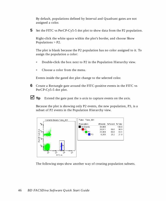
By default, populations defined by Interval and Quadrant gates are not assigned a color.

5 Set the FITC vs PerCP-Cy5-5 dot plot to show data from the P2 population.

Right-click the white space within the plot’s border, and choose Show Populations > P2.

The plot is blank because the P2 population has no color assigned to it. To assign the population a color:

- Double-click the box next to P2 in the Population Hierarchy view.

- Choose a color from the menu.

Events inside the gated dot plot change to the selected color.

6 Create a Rectangle gate around the FITC-positive events in the FITC vs PerCP-Cy5-5 dot plot.

Tip Extend the gate past the x-axis to capture events on the axis.

Because the plot is showing only P2 events, the new population, P3, is a subset of P2 events in the Population Hierarchy view.

The following steps show another way of creating population subsets.



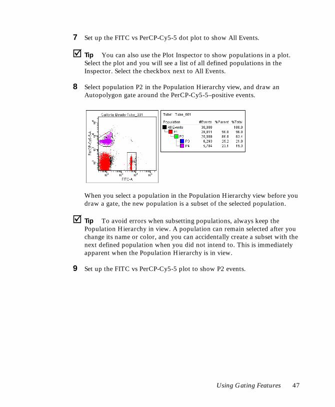
7 Set up the FITC vs PerCP-Cy5-5 dot plot to show All Events.

Tip You can also use the Plot Inspector to show populations in a plot. Select the plot and you will see a list of all defined populations in the Inspector. Select the checkbox next to All Events.

8 Select population P2 in the Population Hierarchy view, and draw an Autopolygon gate around the PerCP-Cy5-5–positive events.

When you select a population in the Population Hierarchy view before you draw a gate, the new population is a subset of the selected population.

Tip To avoid errors when subsetting populations, always keep the Population Hierarchy in view. A population can remain selected after you change its name or color, and you can accidentally create a subset with the next defined population when you did not intend to. This is immediately apparent when the Population Hierarchy is in view.

9 Set up the FITC vs PerCP-Cy5-5 plot to show P2 events.



Using Tethering, Batch Analysis, and Biexponential Display

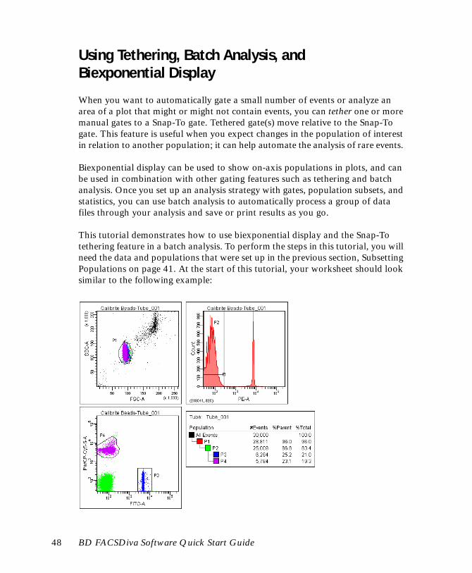
When you want to automatically gate a small number of events or analyze an area of a plot that might or might not contain events, you can tether one or more manual gates to a Snap-To gate. Tethered gate(s) move relative to the Snap-To gate. This feature is useful when you expect changes in the population of interest in relation to another population; it can help automate the analysis of rare events.

Biexponential display can be used to show on-axis populations in plots, and can be used in combination with other gating features such as tethering and batch analysis. Once you set up an analysis strategy with gates, population subsets, and statistics, you can use batch analysis to automatically process a group of data files through your analysis and save or print results as you go.

This tutorial demonstrates how to use biexponential display and the Snap-To tethering feature in a batch analysis. To perform the steps in this tutorial, you will need the data and populations that were set up in the previous section, Subsetting Populations on page 41. At the start of this tutorial, your worksheet should look similar to the following example:



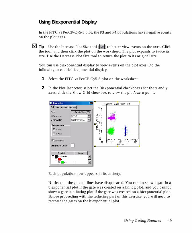
Using Biexponential Display

In the FITC vs PerCP-Cy5-5 plot, the P3 and P4 populations have negative events on the plot axes.

Tip Use the Increase Plot Size tool ( ) to better view events on the axes. Click the tool, and then click the plot on the worksheet. The plot expands to twice its size. Use the Decrease Plot Size tool to return the plot to its original size.

You can use biexponential display to view events on the plot axes. Do the following to enable biexponential display.

1 Select the FITC vs PerCP-Cy5-5 plot on the worksheet.

2 In the Plot Inspector, select the Biexponential checkboxes for the x and y axes; click the Show Grid checkbox to view the plot’s zero point.

Each population now appears in its entirety.

Notice that the gate outlines have disappeared. You cannot show a gate in a biexponential plot if the gate was created on a lin/log plot, and you cannot show a gate in a lin/log plot if the gate was created on a biexponential plot. Before proceeding with the tethering part of this exercise, you will need to recreate the gates on the biexponential plot.



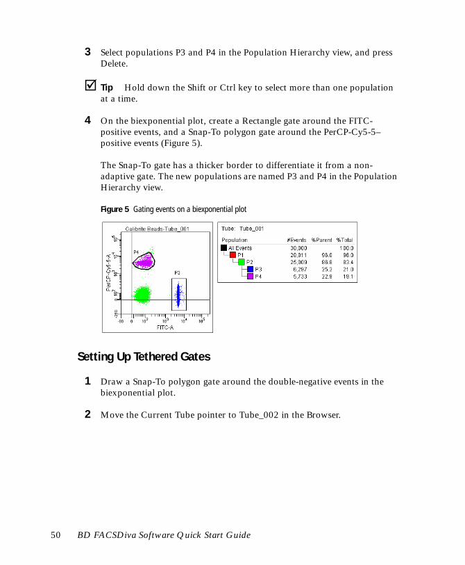
3 Select populations P3 and P4 in the Population Hierarchy view, and press Delete.

Tip Hold down the Shift or Ctrl key to select more than one population at a time.

4 On the biexponential plot, create a Rectangle gate around the FITC-positive events, and a Snap-To polygon gate around the PerCP-Cy5-5–positive events (Figure 5).

The Snap-To gate has a thicker border to differentiate it from a non-adaptive gate. The new populations are named P3 and P4 in the Population Hierarchy view.

Figure 5 Gating events on a biexponential plot

Setting Up Tethered Gates

1 Draw a Snap-To polygon gate around the double-negative events in the biexponential plot.

2 Move the Current Tube pointer to Tube_002 in the Browser.



Notice that the Snap-To gates adjust to encompass their respective populations. However, the P3 gate is now missing some events.

We will use the tethering feature to ensure the gate does not miss events when data in the plot changes.

3 Move the Current Tube pointer back to Tube_001.

4 Select the P3 gate in the plot.

5 In the Inspector, choose P5 from the Tethering drop-down menu.

This tethers the Rectangle gate to the Snap-To gate, so it will move in relation to the gate around the double-negative population.

Notice that the boundary of the tethered gate becomes thicker, and a chain-link icon appears next to the gate label.



6 Move the pointer to Tube_002 in the Browser.

Notice how the tethered gate moves in relation to the Snap-To gate.

7 If necessary, adjust the Rectangle gate so it captures all events.

Performing a Batch Analysis

Now that you have defined and tested your analysis strategy to ensure it works with your data, you are ready to perform a batch analysis. When an analysis includes a plot with biexponential scales, you can process the batch with the same biexponential scales, or change the scaling in relation to the negative events in the data file. The following example shows both options.

1 Right-click the Calibrite Specimen in the Browser, and choose Batch Analysis.

The Batch Analysis dialog box appears.

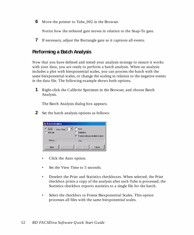
2 Set the batch analysis options as follows:

• Click the Auto option.

• Set the View Time to 5 seconds.

• Deselect the Print and Statistics checkboxes. When selected, the Print checkbox prints a copy of the analysis after each Tube is processed; the Statistics checkbox exports statistics to a single file for the batch.

• Select the checkbox to Freeze Biexponential Scales. This option processes all files with the same biexponential scales.



3 Click Start.

Data for each Tube is shown in the analysis template for 5 seconds before processing of the next Tube begins. All Tubes under the Specimen are processed using the same biexponential scales. When the batch is finished, a message is displayed.

4 Click OK to dismiss the batch completion message.

Note that you can process the batch using scales from any Tube in the batch. To process the batch with a different zero point, do the following.

• Move the Current Tube pointer to Tube_003.

• Right-click the Specimen, and choose Batch Analysis; click Start.

Now, all files are processed using scaling from Tube_003.

NOTICE The scaling for the data files in this example vary extensively for effect. Normally, all samples in a batch are more similar. When performing a batch analysis with biexponential scales, you will need to pick a Tube for the zero point that best represents all files in the batch. Users should validate this feature in their laboratories.

5 (Optional) Repeat the batch analysis with the Freeze Biexponential Scales option deselected.

When you click Start, the following message appears:

NOTICE When a batch analysis includes non-adaptive or non-tethered gates, unfreezing the biexponential scales can cause gated events to fall outside their population boundaries.



Click OK to proceed. Notice that the plot’s zero point fluctuates for each subsequent Tube.

Adjusting the Size of Snap-To Gates

When needed, you can adjust the size of a Snap-To gate to capture a population’s outlying events. Use the results from the previous exercise to try out this feature.

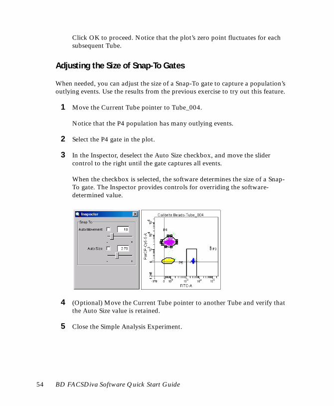
1 Move the Current Tube pointer to Tube_004.

Notice that the P4 population has many outlying events.

2 Select the P4 gate in the plot.

3 In the Inspector, deselect the Auto Size checkbox, and move the slider control to the right until the gate captures all events.

When the checkbox is selected, the software determines the size of a Snap-To gate. The Inspector provides controls for overriding the software-determined value.

4 (Optional) Move the Current Tube pointer to another Tube and verify that the Auto Size value is retained.

5 Close the Simple Analysis Experiment.



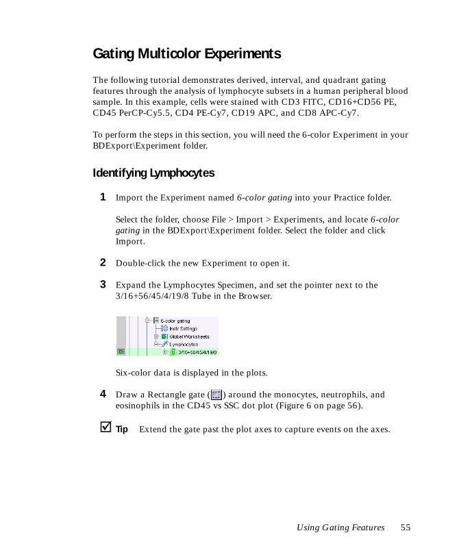
Gating Multicolor Experiments

The following tutorial demonstrates derived, interval, and quadrant gating features through the analysis of lymphocyte subsets in a human peripheral blood sample. In this example, cells were stained with CD3 FITC, CD16+CD56 PE, CD45 PerCP-Cy5.5, CD4 PE-Cy7, CD19 APC, and CD8 APC-Cy7.

To perform the steps in this section, you will need the 6-color Experiment in your BDExport\Experiment folder.

Identifying Lymphocytes

1 Import the Experiment named 6-color gating into your Practice folder.

Select the folder, choose File > Import > Experiments, and locate 6-color gating in the BDExport\Experiment folder. Select the folder and click Import.

2 Double-click the new Experiment to open it.

3 Expand the Lymphocytes Specimen, and set the pointer next to the 3/16+56/45/4/19/8 Tube in the Browser.

Six-color data is displayed in the plots.

4 Draw a Rectangle gate ( ) around the monocytes, neutrophils, and eosinophils in the CD45 vs SSC dot plot (Figure 6 on page 56).

Tip Extend the gate past the plot axes to capture events on the axes.



Figure 6 Gating non-lymphocyte events

5 Use the Population Hierarchy view to rename the population MNEs.

The Population Hierarchy view is part of the imported Experiment. To rename the population, select P1 in the Population Hierarchy view, enter MNEs, and press Return.

Move the gate label off the population in the plot, if needed.

6 Right-click the MNEs population in the Population Hierarchy view and choose Invert Gate.

Inverted gates use the NOT operator to select events outside a defined gate. A new population containing all events except the monocytes, neutrophils, and eosinophils, NOT (MNEs), is added to the Population Hierarchy view. All events in the plot that are not MNEs are colored green.

neutrophils

monocytes

lymphocytes

eosinophils



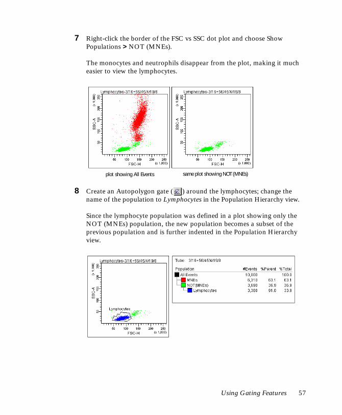
7 Right-click the border of the FSC vs SSC dot plot and choose Show Populations > NOT (MNEs).

The monocytes and neutrophils disappear from the plot, making it much easier to view the lymphocytes.

8 Create an Autopolygon gate ( ) around the lymphocytes; change the name of the population to Lymphocytes in the Population Hierarchy view.

Since the lymphocyte population was defined in a plot showing only the NOT (MNEs) population, the new population becomes a subset of the previous population and is further indented in the Population Hierarchy view.

plot showing All Events same plot showing NOT (MNEs)



Identifying Lymphocyte Subsets

Now, you will create gates to identify CD3+, CD19+, and CD16+56+ populations (T, B, and NK cells, respectively).

Tip To avoid errors when subsetting populations, always keep the Population Hierarchy in view. A population can remain selected after you change its name or color, and you can accidentally create a subset with the next defined population when you did not intend to. This is immediately apparent when the Population Hierarchy is in view.

1 Right-click the Lymphocytes gate in the FSC vs SSC plot and choose Drill Down.

A new FSC vs SSC plot appears, displaying only Lymphocyte events. After gated populations have been defined in a plot, use the Drill Down feature to easily create a plot showing data from only one population.

2 Move the new plot to a clear area on the worksheet.

3 Change the FSC label on the new plot to CD3.

4 Draw an Interval gate ( ) around the CD3+ cells and name the new population T cells.

Note that Interval gates, normally used on histograms, work equally well on dot plots (in a vertical direction).



The newly created population has a checked color box, indicating that the population has no color. Events within an Interval gate retain the color of their parent population (lymphocytes, in this case).

5 Create a CD19 histogram showing the Lymphocytes population.

The CD19 histogram will be used to define B cells. You could also use a CD19 vs SSC dot plot in its place.

6 Draw an Autointerval gate ( ) around the CD19+ cells and name the new population B cells.

An Autointerval gate is like an Autopolygon gate in that a gate is drawn automatically.

7 Right-click in the border of the CD3 vs SSC plot and choose Duplicate.

8 Move the new plot to a clear area on the worksheet.

9 Change the Y axis to CD16+56.

10 Draw a Rectangle gate ( ) around the CD16+56+ cells and name the new population NK cells (Figure 7 on page 60).

Tip Use the biexponential display feature to show events on the plot axes. To turn on biexponential display, select the plot, and select the Biexponential X and Y Axis checkboxes in the Inspector.



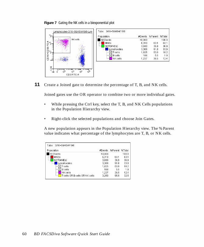
Figure 7 Gating the NK cells in a biexponential plot

11 Create a Joined gate to determine the percentage of T, B, and NK cells.

Joined gates use the OR operator to combine two or more individual gates.

• While pressing the Ctrl key, select the T, B, and NK Cells populations in the Population Hierarchy view.

• Right-click the selected populations and choose Join Gates.

A new population appears in the Population Hierarchy view. The %Parent value indicates what percentage of the lymphocytes are T, B, or NK cells.



Identifying T-Cell Subsets

This section describes how to use quadrant gates to identify T-helper and T-suppressor subsets.

1 Change the color of the T cells in the Population Hierarchy view.

Double-click the checked box in front of the T cell population and select the orange color box. The T cells now change to orange in all plots.

Tip To further subset a population that has no color assigned to it ( ), you must first change the color.

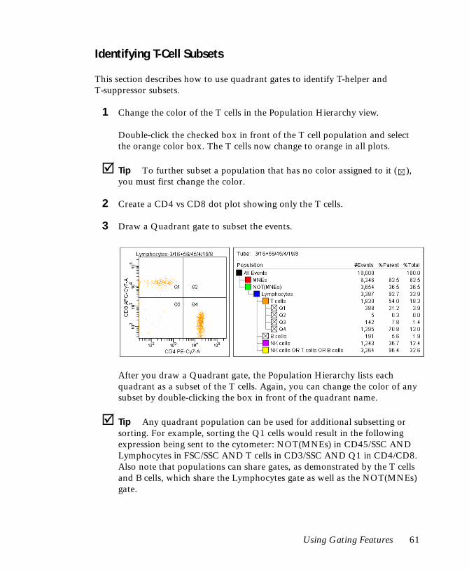
2 Create a CD4 vs CD8 dot plot showing only the T cells.

3 Draw a Quadrant gate to subset the events.

After you draw a Quadrant gate, the Population Hierarchy lists each quadrant as a subset of the T cells. Again, you can change the color of any subset by double-clicking the box in front of the quadrant name.

Tip Any quadrant population can be used for additional subsetting or sorting. For example, sorting the Q1 cells would result in the following expression being sent to the cytometer: NOT(MNEs) in CD45/SSC AND Lymphocytes in FSC/SSC AND T cells in CD3/SSC AND Q1 in CD4/CD8. Also note that populations can share gates, as demonstrated by the T cells and B cells, which share the Lymphocytes gate as well as the NOT(MNEs) gate.



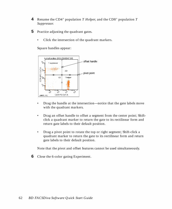
4 Rename the CD4+ population T Helper, and the CD8+ population T Suppressor.

5 Practice adjusting the quadrant gates.

• Click the intersection of the quadrant markers.

Square handles appear:

• Drag the handle at the intersection—notice that the gate labels move with the quadrant markers.

• Drag an offset handle to offset a segment from the center point; Shift-click a quadrant marker to return the gate to its rectilinear form and return gate labels to their default position.

• Drag a pivot point to rotate the top or right segment; Shift-click a quadrant marker to return the gate to its rectilinear form and return gate labels to their default position.

Note that the pivot and offset features cannot be used simultaneously.

6 Close the 6-color gating Experiment.

pivot point

offset handle



Calculating Compensation Using Instrument Setup

The Instrument Setup feature in BD FACSDiva software is designed to automatically calculate spectral overlap values for an experiment, which can save time and eliminate inaccuracies introduced when setting compensation manually. This tutorial shows you how to use the Instrument Setup feature.

Setting Up Compensation Controls

The first step in Instrument Setup is creating the compensation controls.

1 Open Experiment_001, the Experiment you created previously.

If you do not have the Experiment, create it as described in Creating a Folder and an Experiment on page 24.

2 Edit the parameter list.

• If you are connected to the instrument, expand Specimen_001, set the Current Tube pointer next to Tube_001, and edit parameters in the Instrument frame.

• If you are working offline, select the Experiment-level instrument settings and edit parameters in the Inspector.

In the Parameters tab, you can add or delete parameters or change to an alternate parameter. Refer to the BD FACSDiva Software Reference Manual for details.

Tip Use the Parameters tab to choose appropriate parameters and delete unneeded ones before you create compensation controls.

3 Choose Instrument > Instrument Setup > Create Compensation Controls.

Calculating Compensation Using Instrument Setup 63


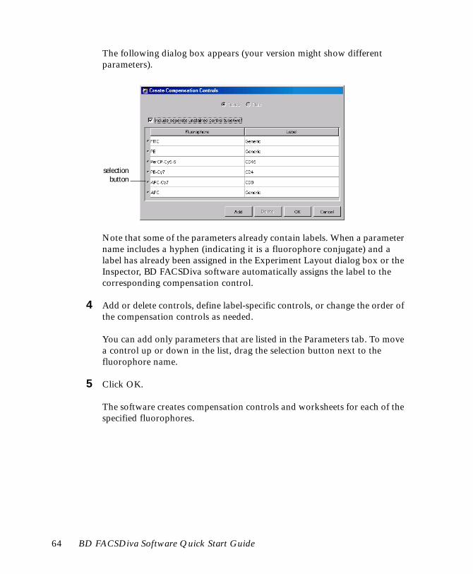
The following dialog box appears (your version might show different parameters).

Note that some of the parameters already contain labels. When a parameter name includes a hyphen (indicating it is a fluorophore conjugate) and a label has already been assigned in the Experiment Layout dialog box or the Inspector, BD FACSDiva software automatically assigns the label to the corresponding compensation control.

4 Add or delete controls, define label-specific controls, or change the order of the compensation controls as needed.

You can add only parameters that are listed in the Parameters tab. To move a control up or down in the list, drag the selection button next to the fluorophore name.

5 Click OK.

The software creates compensation controls and worksheets for each of the specified fluorophores.

selectionbutton



6 Expand the Compensation Controls Specimen to view compensation controls.

Creating an Instrument Configuration

The next step in Instrument Setup is recording data. We have set up an Experiment containing a Compensation Specimen with recorded data you can use to calculate compensation. However, in order to calculate compensation, you must have an instrument configuration that matches the one used to record the data.

Follow these steps to create the required instrument configuration.

1 Choose Instrument > Instrument Configuration.

2 In the Instrument Configuration dialog box, click Add Configuration.

3 In the Instrument Configuration Name dialog box, enter 2 laser, 4 color, and click OK.

NOTICE Make sure the name you enter exactly matches this figure. If the number of spaces or the capitalization differs from this example, you will get an error message when you try to calculate compensation.



4 Select 2 laser, 4 color in the list of instrument configurations, and click the Add Parameter button six times.

This configuration will contain FSC, SSC, and four fluorochromes for a total of six parameters.

Your instrument configuration should look similar to the following:

Configurations are instrument-specific, so your dialog box might have different options than the example shown.

5 Specify the laser and detector, and enter names for each parameter.

You must first assign a detector before you can change a parameter name. Refer to your instrument manual or look at another configuration to find the appropriate laser and detector for each parameter.

To change the laser or detector, click the field in the corresponding column. A drop-down menu appears listing all available choices.

Change the parameter names to FSC, SSC, FITC, PE, PerCP, and APC.

6 If you have a Side Scatter Parameter menu in the upper-right corner of the dialog box, choose the corresponding parameter from the menu.

7 Click OK.

Note that it isn’t necessary to set the 2 laser, 4 color configuration as the current configuration.



Importing Data and Calculating Compensation

Now that you have defined a configuration that matches the one used in our sample Experiment, you are ready to import the Experiment.

You will use the recorded data in this sample Experiment to draw gates and calculate compensation.

1 Select your Practice folder, and import the AutoComp Experiment from the BDExport\Experiment folder.

Choose File > Import > Experiments, and locate the AutoComp Experiment in the dialog box that appears. Select the folder and click Import.

2 Double-click the AutoComp Experiment to open it.

Notice that the Experiment contains a Compensation Specimen and Tubes for four fluorescent parameters.

3 Double-click the Unstained Control Tube to locate the corresponding worksheet.

Notice that compensation Specimens use normal worksheets, rather than global worksheets. (There is no tinting on the tabs.) You can locate data on a normal worksheet by double-clicking the Tube associated with the worksheet.

4 Move the P1 gate to encircle the negative events on the FSC vs SSC dot plot.



5 Right-click the gate boundary and choose Apply to All Compensation Controls.

This applies your gate changes to the worksheets for the remaining compensation controls.

6 Double-click the first Stained Control Tube (FITC Stained Control) to locate the corresponding plots on the worksheet.

7 Ensure that the P2 gate captures all positive events.

The P2 gate is a Snap-To Interval gate, so it should already capture the positive events. If some events are missing, right-click the gate and choose Recalculate.

8 Double-click the next Stained Control Tube in the Browser to locate the corresponding plots on the worksheet.

9 Repeat steps 7 and 8 for the remaining compensation controls.

Once all gates have been set, you are ready to calculate the compensation.

10 Choose Instrument > Instrument Setup > Calculate Compensation.

A dialog box appears where you can enter a name for the compensation Setup.



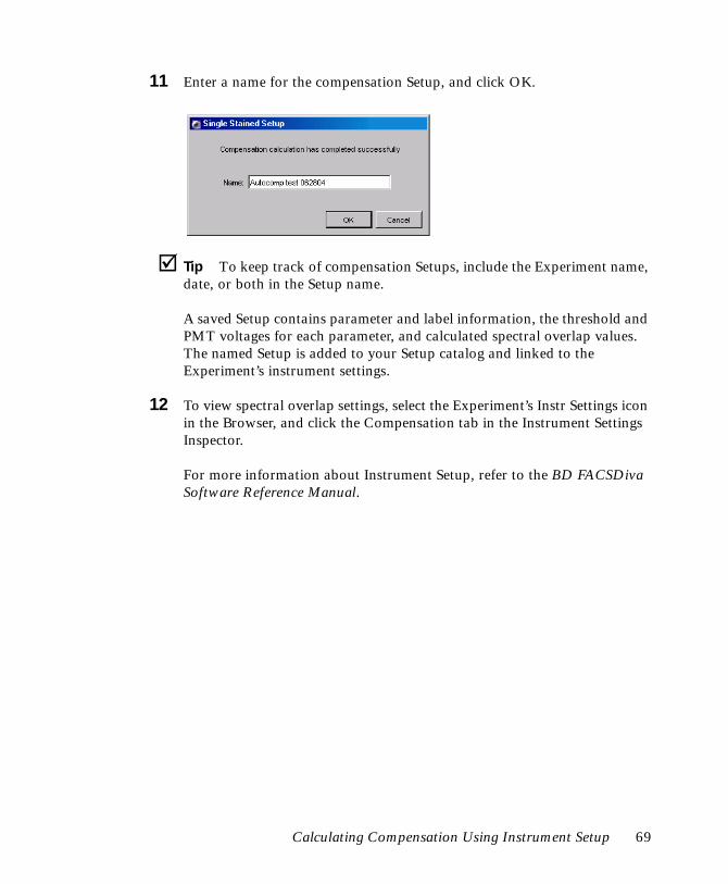
11 Enter a name for the compensation Setup, and click OK.

Tip To keep track of compensation Setups, include the Experiment name, date, or both in the Setup name.

A saved Setup contains parameter and label information, the threshold and PMT voltages for each parameter, and calculated spectral overlap values. The named Setup is added to your Setup catalog and linked to the Experiment’s instrument settings.

12 To view spectral overlap settings, select the Experiment’s Instr Settings icon in the Browser, and click the Compensation tab in the Instrument Settings Inspector.

For more information about Instrument Setup, refer to the BD FACSDiva Software Reference Manual.



Calculating Compensation Manually

When you adjust compensation settings manually, the means for each fluorescence-positive population are compared to the means for its negative population. Appropriate compensation networks are adjusted to align the means.

Tip Compare medians for populations with many outlying events. Compare means when cells are clustered more closely together with few outlying events.

This section describes an alternate method for setting up a compensation matrix using the Copy Spectral Overlap and Paste Spectral Overlap features. Note that compensation calculation is part of instrument settings optimization that typically occurs after you have performed daily quality control and adjusted the voltages and threshold. Refer to your instrument manual for specific instructions.

You will need to import the Manual Comp Experiment to perform the steps in this tutorial. If you haven’t already done so, import the Experiment as described in Importing an Experiment on page 32.

You do not need to be connected to the instrument to perform these exercises. If you are not connected, you will see a plot icon for the Current Tube pointer in the Browser rather than a pointer icon.

Adjusting FITC Compensation

This section describes how to determine spillover coefficients for the FITC fluorochrome. The same procedure is used for the remaining fluorochromes in the Experiment.

1 Open the Manual Comp Experiment, and move the pointer to the FITC Stained Control under the Compensation Controls Specimen.



Data for the FITC tube is shown on the worksheet.

2 Create a Snap-To gate around the singlet events on the FSC vs SSC dot plot.

3 Select the fluorescence plots on the worksheet, right-click either plot border, and choose Show Populations > P1.

Non-singlet events are no longer shown in the plots.

4 Draw an Interval gate around the FITC-positive events on the FITC-A vs PE-A plot; in the Population Hierarchy view, rename the population FITC Positive.

5 Right-click the FITC Positive population in the Population Hierarchy view and choose Invert Gate; rename the NOT (FITC Positive) population Negative (Figure 8 on page 72).

Calculating Compensation Manually 71


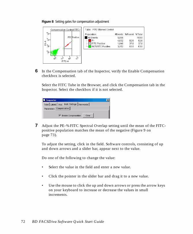
Figure 8 Setting gates for compensation adjustment

6 In the Compensation tab of the Inspector, verify the Enable Compensation checkbox is selected.

Select the FITC Tube in the Browser, and click the Compensation tab in the Inspector. Select the checkbox if it is not selected.

7 Adjust the PE–%FITC Spectral Overlap setting until the mean of the FITC-positive population matches the mean of the negative (Figure 9 on page 73).

To adjust the setting, click in the field. Software controls, consisting of up and down arrows and a slider bar, appear next to the value.

Do one of the following to change the value:

• Select the value in the field and enter a new value.

• Click the pointer in the slider bar and drag it to a new value.

• Use the mouse to click the up and down arrows or press the arrow keys on your keyboard to increase or decrease the values in small increments.



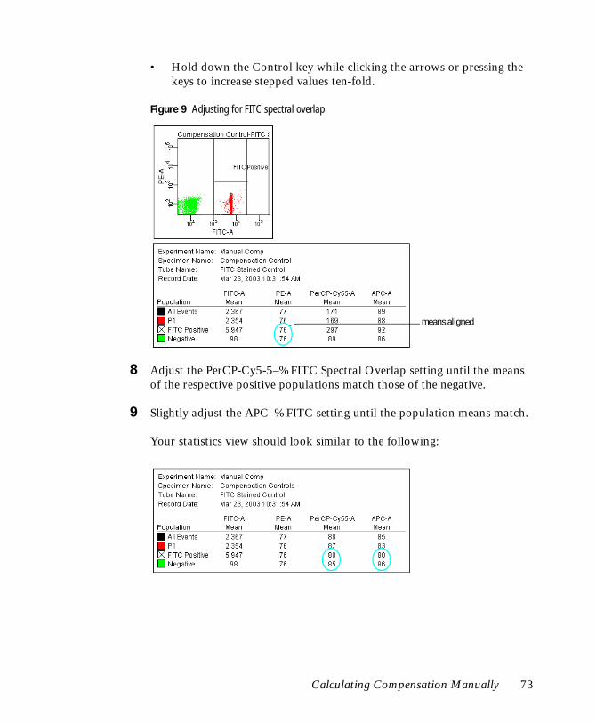
• Hold down the Control key while clicking the arrows or pressing the keys to increase stepped values ten-fold.

Figure 9 Adjusting for FITC spectral overlap

8 Adjust the PerCP-Cy5-5–%FITC Spectral Overlap setting until the means of the respective positive populations match those of the negative.

9 Slightly adjust the APC–%FITC setting until the population means match.

Your statistics view should look similar to the following:

means aligned



Adjusting Compensation for the Remaining Tubes

Repeat the following procedure for each remaining compensation control.

1 Move the Acquisition pointer to the next Tube in the Browser to display its data.

2 Change the plot axes to display the appropriate fluorochromes.

For example, when you are compensating the PE Tube, change the x-axis to PE-A, and the y-axis to FITC-A.

3 Delete the Positive population for the previous fluorochrome from the Population Hierarchy view.

Select the population in the view, and then press the Delete key.

4 Draw an Interval gate around the fluorescence-positive cells; rename the population (fluorochrome name) Positive.

5 Right-click the Positive population in the Population Hierarchy view and choose Invert Gate; rename the NOT (Positive) population Negative.

Your worksheet should contain objects similar to those shown in Figure 8 on page 72.

6 Verify the Enable Compensation checkbox is selected and adjust the appropriate compensation networks to remove spectral overlap from the respective detectors.

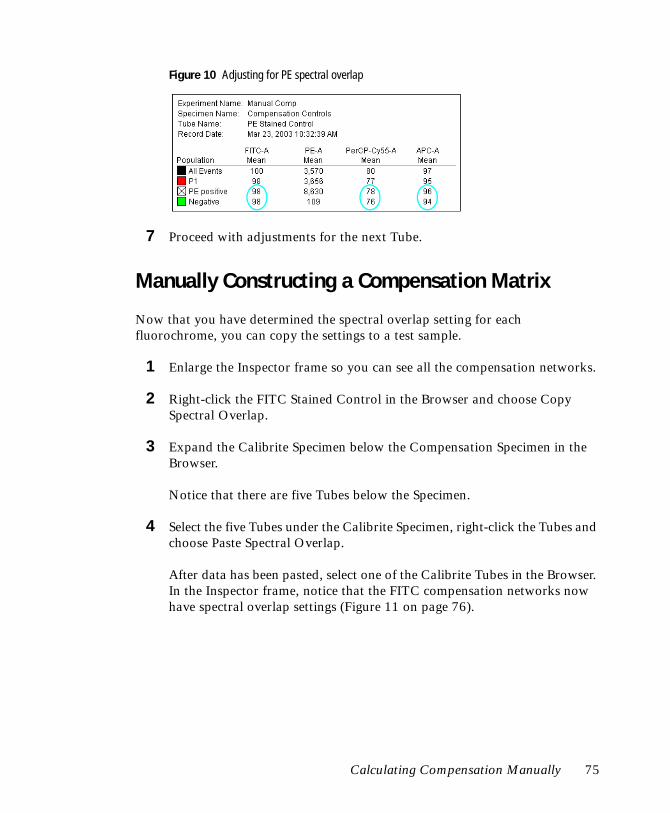
For example, for PE compensation, adjust FITC–%PE and PerCP-Cy5.5–%PE compensation until the means for each fluorescent parameter match as closely as possible (Figure 10).

Tip Use the Ctrl key and the arrow keys on the keyboard to quickly change the settings.



Figure 10 Adjusting for PE spectral overlap

7 Proceed with adjustments for the next Tube.

Manually Constructing a Compensation Matrix

Now that you have determined the spectral overlap setting for each fluorochrome, you can copy the settings to a test sample.

1 Enlarge the Inspector frame so you can see all the compensation networks.

2 Right-click the FITC Stained Control in the Browser and choose Copy Spectral Overlap.

3 Expand the Calibrite Specimen below the Compensation Specimen in the Browser.

Notice that there are five Tubes below the Specimen.

4 Select the five Tubes under the Calibrite Specimen, right-click the Tubes and choose Paste Spectral Overlap.

After data has been pasted, select one of the Calibrite Tubes in the Browser. In the Inspector frame, notice that the FITC compensation networks now have spectral overlap settings (Figure 11 on page 76).



Figure 11 Pasting overlap settings for the FITC Tube

5 Copy Spectral Overlap settings for each compensation control in turn, and paste the settings to the five Tubes under the Calibrite Specimen.

When you finish pasting settings for the APC Stained Control, the compensation matrix should be complete.

Tip Use the Paste Spectral Overlap with Zeros command in cases where you are pasting spectral overlap settings to a Tube that already has a complete set of spectral overlap values. Refer to the BD FACSDiva Software Reference Manual for more information.



Maintaining the Database

Now that you have finished these tutorials, save space in your database by deleting your Practice folder and the Experiments within it.

1 Close any open Experiment.

All Experiments must be closed before you can delete the folder containing them.

2 Select the Practice folder and press the Delete key.

3 Click OK in the dialog that appears.

Deleted Experiments are removed from the Browser and from the database on the D:\ drive.

Maintaining the Database 77



Date post:	04-Feb-2022
Category:	Documents
Upload:	others
View:	18 times
Download:	0 times

BD FACSDiva Software Quick Start Guide

Documents