Beauty in photoproduction at HERA II with the ZEUS detector · Chapter 2 begins with a description...

Beauty in photoproduction

at HERA II

with the ZEUS detector

Sarah Boutle

University College London

August 2009

PhD thesis

Thesis submitted to University College London

in fulfilment of the requirements for the award of

the degree of Doctor of Philosophy

1

I, Sarah Boutle confirm that the work presented in this thesis is my own. Where information has

been derived from other sources, I confirm that this has been indicated in the thesis.

2

Abstract

The production of beauty quarks in ep collisions should be accurately calculable in perturbative

Quantum Chromodynamics (QCD) since the large mass of the b quark provides a hard scale.

Therefore it is interesting to compare such predictions to results using photoproduction events

where a low-virtuality photon, emitted by the incoming lepton, collides with a parton from the

incoming proton. A measurement of beauty in photoproduction has been made at HERA with the

ZEUS detector using an integrated luminosity of 126 pb−1. Beauty was identified in events with

a muon in the final state by using the transverse momentum of the muon relative to the closest

jet. Lifetime information from the silicon vertex detector was also used; the impact parameter

of the muon with respect to the primary vertex was exploited to discriminate between signal

and background. Cross sections for beauty production as a function of the muon and the jet

variables were measured and compared to QCD predictions and to previous measurements. The

data were found to be well described by the predictions from next-to-leading-order QCD. The dijet

sample of beauty photoproduction events was also used to study higher-order QCD topologies. At

leading order, the two jets in the event are produced back-to-back in azimuthal angle, such that

∆φjj = φj1 − φj2 = π. Additional soft radiation causes small azimuthal decorrelations, whilst

∆φjj significantly lower than π is evidence of additional hard radiation. In this thesis, the cross

section versus ∆φjj for beauty photoproduction and the comparison to NLO QCD predictions and

Monte Carlo models are presented.

3

To my parents

4

Outline

An analysis of beauty production in ep collisions at HERA is presented in this thesis. The measure-

ment used data collected in 2005 using the ZEUS detector and is published in [1]. In chapter 1 a

theoretical overview of ep scattering and the processes under study in this thesis is given. Chapter

2 begins with a description of theoretical calculations of beauty production and then moves on

to give a summary of previous relevant experimental results. The HERA collider and the ZEUS

detector are described in chapter 3. In chapter 4, the reconstruction of the event objects to be

used in this analysis is described while chapter 5 describes how interesting events were selected.

Chapter 5 also describes the Monte Carlo samples used. Chapter 6 gives details of the analysis

method used to identify beauty events and, finally, the results are given in chapter 7.

5

Contents

1 Quantum chromodynamics and ep scattering 16

1.1 Electron proton scattering . . . . . . . . . . . . . . . . . . . . . . . . . . . . . . . . 16

1.2 The quark parton model . . . . . . . . . . . . . . . . . . . . . . . . . . . . . . . . . 17

1.3 The improved parton model . . . . . . . . . . . . . . . . . . . . . . . . . . . . . . . 19

1.4 Evolution of parton densities . . . . . . . . . . . . . . . . . . . . . . . . . . . . . . 19

1.5 Photoproduction . . . . . . . . . . . . . . . . . . . . . . . . . . . . . . . . . . . . . 20

1.6 Direct and resolved photon processes . . . . . . . . . . . . . . . . . . . . . . . . . . 21

2 Beauty production 24

2.1 Photoproduction of heavy quarks at HERA . . . . . . . . . . . . . . . . . . . . . . 24

2.2 Perturbative formalism of the photoproduction of heavy quarks . . . . . . . . . . . 25

2.3 NLO QCD photoproduction calculations . . . . . . . . . . . . . . . . . . . . . . . . 26

2.4 Monte Carlo simulations . . . . . . . . . . . . . . . . . . . . . . . . . . . . . . . . . 26

2.4.1 Event generators . . . . . . . . . . . . . . . . . . . . . . . . . . . . . . . . . 27

2.4.2 Hadronisation in PYTHIA . . . . . . . . . . . . . . . . . . . . . . . . . . . 27

2.5 An overview of previous measurements . . . . . . . . . . . . . . . . . . . . . . . . . 27

2.5.1 Beauty production at HERA . . . . . . . . . . . . . . . . . . . . . . . . . . 28

2.5.2 Beauty production at hadron colliders . . . . . . . . . . . . . . . . . . . . . 30

6

2.5.3 Beauty production in γγ interactions . . . . . . . . . . . . . . . . . . . . . . 31

2.5.4 Dijet correlation measurements at ZEUS . . . . . . . . . . . . . . . . . . . . 31

3 HERA and the ZEUS detector 38

3.1 HERA . . . . . . . . . . . . . . . . . . . . . . . . . . . . . . . . . . . . . . . . . . . 38

3.1.1 The HERA upgrade . . . . . . . . . . . . . . . . . . . . . . . . . . . . . . . 39

3.1.2 The HERA injection system . . . . . . . . . . . . . . . . . . . . . . . . . . . 39

3.2 The ZEUS detector . . . . . . . . . . . . . . . . . . . . . . . . . . . . . . . . . . . . 40

3.2.1 The ZEUS coordinate system . . . . . . . . . . . . . . . . . . . . . . . . . . 40

3.2.2 The micro-vertex detector . . . . . . . . . . . . . . . . . . . . . . . . . . . . 41

3.2.3 The central tracking detector . . . . . . . . . . . . . . . . . . . . . . . . . . 42

3.2.4 The Uranium calorimeter . . . . . . . . . . . . . . . . . . . . . . . . . . . . 43

3.2.5 Muon chambers . . . . . . . . . . . . . . . . . . . . . . . . . . . . . . . . . . 44

3.2.6 Luminosity measurement . . . . . . . . . . . . . . . . . . . . . . . . . . . . 45

3.2.7 Trigger system . . . . . . . . . . . . . . . . . . . . . . . . . . . . . . . . . . 46

4 Event Reconstruction 48

4.1 Track and vertex reconstruction . . . . . . . . . . . . . . . . . . . . . . . . . . . . . 48

4.2 Beam spot . . . . . . . . . . . . . . . . . . . . . . . . . . . . . . . . . . . . . . . . . 49

4.3 Muon finding . . . . . . . . . . . . . . . . . . . . . . . . . . . . . . . . . . . . . . . 49

4.4 Hadronic system reconstruction . . . . . . . . . . . . . . . . . . . . . . . . . . . . . 50

4.5 Jet finding . . . . . . . . . . . . . . . . . . . . . . . . . . . . . . . . . . . . . . . . . 51

5 Event Selection 53

5.1 Trigger selection . . . . . . . . . . . . . . . . . . . . . . . . . . . . . . . . . . . . . 53

7

5.1.1 Trigger efficiency . . . . . . . . . . . . . . . . . . . . . . . . . . . . . . . . . 54

5.2 Selection of photoproduction events . . . . . . . . . . . . . . . . . . . . . . . . . . 54

5.2.1 Rejection of reconstructed electron . . . . . . . . . . . . . . . . . . . . . . . 55

5.3 Reconstruction of y . . . . . . . . . . . . . . . . . . . . . . . . . . . . . . . . . . . . 56

5.4 Rejection of beam gas events . . . . . . . . . . . . . . . . . . . . . . . . . . . . . . 56

5.5 Event selection . . . . . . . . . . . . . . . . . . . . . . . . . . . . . . . . . . . . . . 56

5.6 Monte Carlo samples . . . . . . . . . . . . . . . . . . . . . . . . . . . . . . . . . . . 57

5.6.1 Beauty event simulation . . . . . . . . . . . . . . . . . . . . . . . . . . . . . 57

5.6.2 Charm event simulation . . . . . . . . . . . . . . . . . . . . . . . . . . . . . 58

5.6.3 Light flavour event simulation . . . . . . . . . . . . . . . . . . . . . . . . . . 58

5.7 Muon efficiency corrections . . . . . . . . . . . . . . . . . . . . . . . . . . . . . . . 58

5.8 Control distributions . . . . . . . . . . . . . . . . . . . . . . . . . . . . . . . . . . . 59

6 Beauty quark identification 61

6.1 The p relT method . . . . . . . . . . . . . . . . . . . . . . . . . . . . . . . . . . . . . 61

6.2 The impact parameter method . . . . . . . . . . . . . . . . . . . . . . . . . . . . . 62

6.3 Comparison between data and MC . . . . . . . . . . . . . . . . . . . . . . . . . . . 64

6.3.1 p relT correction . . . . . . . . . . . . . . . . . . . . . . . . . . . . . . . . . . 64

6.3.2 Impact parameter smearing . . . . . . . . . . . . . . . . . . . . . . . . . . . 65

6.4 Extraction of the beauty fraction . . . . . . . . . . . . . . . . . . . . . . . . . . . . 66

7 Cross-section measurement 69

7.1 Purities, efficiencies and acceptance corrections . . . . . . . . . . . . . . . . . . . . 70

7.2 Determination of the systematic uncertainties . . . . . . . . . . . . . . . . . . . . . 70

7.3 Theoretical predictions . . . . . . . . . . . . . . . . . . . . . . . . . . . . . . . . . . 73

8

7.4 Total cross section . . . . . . . . . . . . . . . . . . . . . . . . . . . . . . . . . . . . 74

7.5 Muon variable differential cross sections . . . . . . . . . . . . . . . . . . . . . . . . 74

7.6 Dijet differential cross sections . . . . . . . . . . . . . . . . . . . . . . . . . . . . . 74

8 Conclusions 79

9 Appendix A: Purities, efficiencies and acceptance correction factors 81

10 Appendix B: Systematic uncertainites 84

9

List of Figures

1.1 (a) Neutral current and (b) charged current interactions. . . . . . . . . . . . . . . 17

1.2 The reduced cross section σr(x,Q2) as a function of Q2 for fixed values of x. Results

from fixed target experiments and the combined ZEUS-H1 HERA I measurements

are compared to an NLO QCD fit from each of the experiments, H12000PDF and

ZEUS-JETS. . . . . . . . . . . . . . . . . . . . . . . . . . . . . . . . . . . . . . . . 18

1.3 The first order splitting functions Pij used in the DGLAP equations. . . . . . . . 20

1.4 Leading order direct ((a) and (b)) and examples of resolved ((c) and (d)) photopro-

duction processes. . . . . . . . . . . . . . . . . . . . . . . . . . . . . . . . . . . . . 22

1.5 Distribution of xobsγ in dijet events for ZEUS data compared with Herwig with (solid

line) and without (dotted line) the inclusion of a model for multi-parton interactions

(MPI) and also compared to Pythia with MPI (dashed line). The shaded area

represents the direct photon events generated by Herwig. Also shown is a vertical

line which defines the experimental distinction between direct and resolved photon

events. . . . . . . . . . . . . . . . . . . . . . . . . . . . . . . . . . . . . . . . . . . 23

2.1 General diagrams for (a) direct and (b) resolved photoproduction. . . . . . . . . . 33

2.2 General structure of the generation of a Monte Carlo event involving a positron-

proton collision. . . . . . . . . . . . . . . . . . . . . . . . . . . . . . . . . . . . . . 33

2.3 Illustration of the Lund string model in which qq pair is joined together by a colour

flux tube which splits at some energy density to form a new qq pair. . . . . . . . . 33

10

2.4 Differential cross sections as a function of pseudorapidity, ηµ, (left) and transverse

momentum, pµT , (right) of the muon for beauty photoproduction in dijet events,

measured by the ZEUS collaboration. The data are compared to predictions from

Pythia and Cascade MC as well as to NLO QCD calculations with and without

factors applied to correct for hadronisation effects (see Sec. 7.3). . . . . . . . . . . 34

2.5 Differential cross sections as a function of pseudorapidity, ηµ, (left) and transverse

momentum, pµT , (right) of the muon for beauty photoproduction in dijet events,

measured by the H1 collaboration. The measurements are compared to predictions

from Pythia and Cascade MC as well as to NLO QCD calculations with and

without factors applied to correct for hadronisation effects (see Sec. 7.3). . . . . . 34

2.6 Differential cross sections as a function of xjetsγ in dijet events with a muon measured

by the ZEUS collaboration (left) and the H1 collaboration (right). The data are

compared to predictions from Pythia and Cascade MC as well as to NLO QCD

calculations. . . . . . . . . . . . . . . . . . . . . . . . . . . . . . . . . . . . . . . . 34

2.7 Differential cross sections as a function of the transverse momentum, peT , (left) and

pseudorapidity, ηe, (right) of the electron for beauty photoproduction in dijet events.

The measurements are compared to the predictions from Pythia as well as to NLO

QCD calculations corrected for hadronisation effects. . . . . . . . . . . . . . . . . 35

2.8 Differential beauty dijet photoproduction cross sections as a function of the trans-

verse momentum of the leading jet, dσ/dpjet1T , (left) and as a function of the mean

pseudorapidity of the two jets, dσ/dη, (right). The measurements are compared to

the absolute predictions of Pythia and Cascade as well as to NLO QCD calcula-

tions corrected for hadronisation effects. . . . . . . . . . . . . . . . . . . . . . . . . 35

2.9 Summary of beauty photoproduction measurements at HERA. Measurements de-

scribed in this section are shown in red and the analysis which forms the sub-

ject of this thesis is shown by the blue markers. The data are compared to NLO

QCD predictions from the FMNR program with two different choices of scale:

µ2 = 1/4(m2 + p2T ) (solid line) and µ2 = m2 + p2

T (dotted line). . . . . . . . . . . 35

2.10 Beauty production cross section measurements made at the Tevatron: (a) as a

function of pbT , made by the CDF and D0 collaborations using RUN I data, and

(b) as a function of pT of J/Ψ from B decays using RUN II data by the the CDF

collaboration. . . . . . . . . . . . . . . . . . . . . . . . . . . . . . . . . . . . . . . 36

11

2.11 Charm (upper) and beauty (lower) production cross sections measured by the L3

collaboration in γγ interactions at LEP. The solid line represents the NLO QCD

prediction for the sum of the direct and single-resolved processes while the dashed

line represents the direct-process contribution. . . . . . . . . . . . . . . . . . . . . 36

2.12 Cross section of dσ/d∆φjj separated into ((a) and (c)) direct enriched (xobsγ > 0.75)

and ((b) and (d)) resolved enriched (xobsγ < 0.75) samples. In (a) and (b) the data

are compared to NLO QCD predictions (blue band). The beauty component is also

shown in red. In (c) and (d) the data are compared to Herwig (red line) and

Pythia (dashed blue line) MC models. . . . . . . . . . . . . . . . . . . . . . . . . 37

2.13 Cross section of dσ/d∆φjj separated into (a) direct enriched (xobsγ > 0.75) and (b)

resolved enriched (xobsγ < 0.75) samples. The data are compared to NLO QCD

predictions calculated using the AFG04 photon PDF. The data are compared to

Herwig (dashed red line) and Pythia (dashed blue line) MC models normalised

by the factors given. . . . . . . . . . . . . . . . . . . . . . . . . . . . . . . . . . . . 37

3.1 Aerial photograph of the Volkspark in Hamburg, Germany showing the locations of

the HERA accelerator and the pre-accelerator, PETRA. . . . . . . . . . . . . . . . 38

3.2 Luminosity delivered by HERA during the different running periods. . . . . . . . 39

3.3 Diagram of the HERA ring with an enlargement of the pre-accelarator, PETRA,

and the injection system. . . . . . . . . . . . . . . . . . . . . . . . . . . . . . . . . 39

3.4 Cross section of the ZEUS detector along the beam direction. . . . . . . . . . . . 41

3.5 Cross section of the ZEUS detector perpendicular to the beam direction. . . . . . 41

3.6 ZEUS coordinate system. . . . . . . . . . . . . . . . . . . . . . . . . . . . . . . . . 41

3.7 x-y cross section of the barrel MVD. . . . . . . . . . . . . . . . . . . . . . . . . . . 42

3.8 (a) Two half-modules of the MVD and (b) cut-away showing the whole MVD situ-

ated inside the CTD and the positions of the barrel ladders and forward wheels. . 42

3.9 (a) r-φ cross-section through the CTD, showing 9 superlayers, and (b) the layout of

a typical cell showing ionisation drift paths. . . . . . . . . . . . . . . . . . . . . . 43

3.10 Schematic of the ZEUS Uranium calorimeter in the x− z plane. . . . . . . . . . . 44

3.11 The different configurations of the towers found in the FCAL, BCAL and RCAL. 44

12

3.12 An exploded view of the barrel and rear muon chambers. . . . . . . . . . . . . . . 45

3.13 Schematic of the photon calorimeter luminosity monitor. . . . . . . . . . . . . . . 46

3.14 Schematic of the luminosity spectrometer. . . . . . . . . . . . . . . . . . . . . . . 46

4.1 Illustration of the parameters used in the VCTRACK track fit. . . . . . . . . . . 48

4.2 Schematic diagram of the formation of cell islands in the calorimeter. . . . . . . . 51

5.1 Efficiency of trigger slot HFL5 for data (points) and MC (solid line) as a function

of (a) pT and (b) η of the second jet and the ratio of data and MC efficiencies also

as a function of (c) pT and (d) η of the second jet. . . . . . . . . . . . . . . . . . . 55

5.2 Efficiency of trigger slot HFL13 for data (points) and MC (solid line) as a function

of (a) pT and (b) η of the muon and the ratio of data and MC efficiencies as a

function of (c) pT and (d) η of the muon. . . . . . . . . . . . . . . . . . . . . . . . 55

5.3 Distributions of (a) pµT , (b) ηµ, (c) pµ-j

T , (d) ηµ-j and (e) xjjγ . The data are compared

to a mixture of beauty (shaded histogram), charm (dotted line) and light flavour

(dashed line) Pythia MC predictions, combined according to the fractions given by

the two-dimensional p relT -δ fit. The total MC distribution is shown as the solid line.

The kinematic region is restricted to pµT > 1.5 GeV (pµ

T > 2.5 GeV) for (a)((b)-(e)). 60

6.1 Illustration of the p relT variable. . . . . . . . . . . . . . . . . . . . . . . . . . . . . 62

6.2 Distributions of (a) p relT and (b) the muon impact parameter, δ. The data are

compared to a mixture of beauty (shaded histogram), charm (dotted line) and light

flavour(dashed line) Pythia MC samples. The total MC distribution is shown as

the solid line. The relative contributions of beauty, charm and light flavour were

mixed according to the fractions measured in this analysis as described in Sec.6.4. 63

6.3 Illustration of the signed impact parameter. . . . . . . . . . . . . . . . . . . . . . 63

6.4 (a) p relT distribution for inclusive dijet samples of data and PYTHIA MC events

(normalised to the data). (b) The ratio of data to MC events as a function of p relT . 65

6.5 MC impact parameter distributions (blue histograms) compared to the data (black

points) in bins of pT (the bin range range for each plot in GeV is given in the

brackets). [2, 3] . . . . . . . . . . . . . . . . . . . . . . . . . . . . . . . . . . . . . . 66

13

6.6 MC impact parameter distributions (blue histograms), after the application of smear-

ing correction, compared to the data (black points) in bins of pT (the bin range range

for each plot in GeV is given in the brackets). [2, 3]. . . . . . . . . . . . . . . . . . 66

6.7 Fit of MC distributions to a data distribution of p relT in bins of δ. . . . . . . . . . 67

6.8 Contours of 68% probability in the plane defined by the beauty and charm fractions.

The results of the χ2 fit to the two-dimensional p relT -δ distribution and to the p rel

T

and δ-only distributions are shown. The diagonal line shows the boundary of the

physical region in which the fractions of b, c and LF are positive. . . . . . . . . . 68

7.1 Purity, p, efficiency, ǫ and acceptance correction factor, A, for the differential cross

section as a function of pµT . . . . . . . . . . . . . . . . . . . . . . . . . . . . . . . . 70

7.2 (a) The factors used to reweight the MC taken from the ratio of the numbers of data

and MC events in bins of ηµ. (b) Comparison of ηµ control distribution for data

and MC for beauty-enriched samples obtained by the requirement of p relT > 2 GeV 71

7.3 dσ

dxjjγ

for data and nominal Pythia MC samples. Also shown are dσ

dxjjγ

for Pythia

MC samples in which (a) the contribution of flavour-excitation events was varied

by +100%/− 50% and simultaneously the contribution of gg → bb, qq → bb events

was varied by − 50%/ + 100% and (b) the contribution of γg → bb processes was

decreased by 20% and all other processes were increased by +100% . . . . . . . . 72

7.4 Differential cross section as a function (a) pµT , (b) ηµ, (c) pµ−j

T and (d) ηµ−j for

Q2 < 1 GeV2, 0.2 < y < 0.8, pj1,j2T > 7, 6 GeV, |ηj1,j2 | < 2.5, and −1.6 < ηµ < 1.3.

For the pµT cross section, the kinematic region is defined as pµ

T > 1.5 GeV and as

pµT > 2.5 GeV for all other cross sections. The filled circles show the results from this

analysis and the open circles show the results from the previous ZEUS measurement.

The inner error bars are statistical uncertainties while the external bars show the

statistical and systematic uncertainties added in quadrature. The band represents

the NLO QCD predictions with their uncertainties. The Pythia MC predictions

are also shown (dashed line). . . . . . . . . . . . . . . . . . . . . . . . . . . . . . . 75

14

7.5 Differential cross sections as a function of (a) xjjγ and (b) ∆φjj of the jet-jet system

and ∆φjj for (c) direct- and (d) resolved-enriched samples for Q2 < 1 GeV2, 0.2 <

y < 0.8, pj1,j2T > 7, 6 GeV, ηj1,j2 < 2.5, pµ

T > 2.5 GeV and −1.6 < ηµ < 1.3.

The inner error bars are statistical uncertainties while the external bars show the

statistical and systematic uncertainties added in quadrature. The band represents

the NLO QCD predictions with their uncertainties. The Pythia MC predictions

are also shown (dashed line). . . . . . . . . . . . . . . . . . . . . . . . . . . . . . . 76

7.6 Compilation of HERA measurements of the differential cross section for b-quark

production as a function of pbT . The measurement in this thesis is represented by

the open red triangles. . . . . . . . . . . . . . . . . . . . . . . . . . . . . . . . . . 77

9.1 Purities, efficiencies and acceptance correction factors for the differential cross sec-

tions as functions of pµT and ηµ. . . . . . . . . . . . . . . . . . . . . . . . . . . . . 81


tions as functions of pµ−jT and ηµ−j . . . . . . . . . . . . . . . . . . . . . . . . . . . 82


tions as functions of ∆φjj and xjjγ . . . . . . . . . . . . . . . . . . . . . . . . . . . 82


tions as functions of ∆φjj for direct-enriched (xjjγ > 0.75) and resolved-enriched

(xjjγ < 0.75) samples. . . . . . . . . . . . . . . . . . . . . . . . . . . . . . . . . . . 83

10.1 Fractional systematic uncertainty due to the muon acceptance. . . . . . . . . . . . 85

10.2 Fractional systematic uncertainty due to the energy scale. . . . . . . . . . . . . . 85

10.3 Fractional systematic uncertainty due to the MVD efficiency. . . . . . . . . . . . . 86

10.4 Fractional systematic uncertainty due to the dijet trigger efficiency. . . . . . . . . 86

10.5 Fractional systematic uncertainty due to the ηµ MC description. . . . . . . . . . . 87

10.6 Fractional systematic uncertainty due to the impact parameter correction. . . . . 87

10.7 Fractional systematic uncertainty due to varying the light flavour background p relT

correction. . . . . . . . . . . . . . . . . . . . . . . . . . . . . . . . . . . . . . . . . 88

10.8 Fractional systematic uncertainty due to varying the charm background p relT correc-

tion. . . . . . . . . . . . . . . . . . . . . . . . . . . . . . . . . . . . . . . . . . . . 88

15

10.9 Fractional systematic uncertainty due to the variation of the flavour excitation pro-

cesses by +100%/ − 50% and the contribution of gg → bb, qq → bb events by

− 50%/+ 100% simultaneously. . . . . . . . . . . . . . . . . . . . . . . . . . . . . 89

10.10Fractional systematic uncertainty due to decreasing the contribution of γg → bb

processes in Pythia by 20% and increasing all other processes by +100%. . . . . 89

10.11Total fractional systematic uncertainty found by summing the individual contribu-

tions in quadrature. . . . . . . . . . . . . . . . . . . . . . . . . . . . . . . . . . . . 90

16

List of Tables

5.1 Cross sections and luminosities of the MC samples used in this thesis. . . . . . . . 58

7.1 Differential muon cross section as a function of pµT and ηµ. For further details

see text. The multiplicative hadronisation correction, Chad, applied to the NLO

prediction is shown in the last column. . . . . . . . . . . . . . . . . . . . . . . . . 75

7.2 Differential cross section for jets associated with a muon as a function of pµ-jT and

ηµ-j . For further details see text. . . . . . . . . . . . . . . . . . . . . . . . . . . . 75

7.3 Differential cross section as a function of xjjγ . For further details see text. . . . . . 76

7.4 Differential muon cross section as a function of ∆φjj for all xjjγ and for xjj

γ > (<)0.75.

For further details see text. . . . . . . . . . . . . . . . . . . . . . . . . . . . . . . . 76

7.5 Differential cross section for b-quark production as a function of pbT as measured in

this analysis. . . . . . . . . . . . . . . . . . . . . . . . . . . . . . . . . . . . . . . . 78

17

Chapter 1

Quantum chromodynamics and ep

scattering

Quantum Chromodynamics (QCD) is the theory of the strong interaction, a fundamental force

which governs the interactions of particles which possess colour charge known as quarks and glu-

ons, the constituents of hadrons such as protons or neutrons. The strength of the interaction,

characterised by the strong coupling constant, αs, increases with distance, a phenomenon known

as asymptotic freedom. As a consequence, quarks can only exist in bound states, a property known

as colour confinement.

Studying ep scattering at HERA provides a good means by which to test the theory of QCD. For

large momentum transfer, it is possible to calculate QCD processes accurately using a perturbative

expansion in αs. This large momentum transfer is known as a hard scale which can also be defined

as the transverse energy of a jet or the mass of a heavy quark. The measurements made can

therefore be used to verify predictions made by such calculations.

1.1 Electron proton scattering

The interaction of an electron and a proton at leading order (LO) occurs with the exchange of

a photon, through the electromagnetic force, or a Z0/W± boson, through the weak force. Such

interactions can be classified into 2 types: neutral and charged current processes which are mediated

by the photon/Z0 and W± respectively and are shown in Fig. 1.1.

18

1.1. Electron proton scattering Chapter 1

e+_ (k) e+_ (k′)

γ, Z0(q)

P(p) X(p′)

(a)

e+_ (k) νν (k′)

W +_ (q)

P(p) X(p′)

(b)

Figure 1.1: (a) Neutral current and (b) charged current interactions.

We can define the kinematics of such processes using the four-momenta of the incoming and the

scattered lepton, k and k′, and the four-momenta of the proton, P , and the exchanged boson,

q = k′ − k. The scattering process can therefore be described by the following quantities:

Q2 = −q2 = (k − k′)2, (1.1)

y =P · qP · k , (1.2)

x =Q2

2P · q . (1.3)

Q2 is the virtuality of the exchanged boson and can be seen as a measure of the resolving power

of the probe where larger values of Q2 can resolve smaller objects. The variables y and x are the

Bjorken scaling variables where y is the fraction of the lepton energy which is transferred to the

interaction in the rest frame of the proton and x is the fraction of the proton momentum carried

by the struck quark. These quantities are related to the square of the centre of mass energy, s, by:

Q2 = sxy. (1.4)

For Q2 ≫ ΛQCD where ΛQCD ≃ 0.2 GeV, the scale is provided by Q2 itself and so perturbative

calculations can be performed. These events are known as Deep Inelastic Scattering (DIS) events.

19

Chapter 1 1.2. The quark parton model

When Q2 ∼ 0 GeV2, the electron scatters through a very small angle and the boson exchanged

is an almost real photon. This process is referred to as photoproduction. In this case, Q2 cannot

be used to define a hard scale and so quantities such as the transverse momentum of the jet or

the mass of the quark, as in heavy quark production, can be used so that measurements can be

compared to theoretical calculations.

1.2 The quark parton model

In the quark parton model, the proton is assumed to be composed of point-like free objects called

partons. In this way, the inelastic electron-proton scattering process can be described in terms

of the elastic scattering of the electron with a parton, i, and the probability, fi(x) of finding this

parton with momentum, x, inside the proton, known as the Parton Distribution Function (PDF).

The neutral current cross section is given by

dσ2

dQ2dx=

4πα2

xQ4

[

y2

22xF1 ∓ (1 − (1 − y)2)F2 ∓

(

y − y2

2

)

xF3

]

, (1.5)

and using FL = F2 − 2xF1,

dσ2

dQ2dx=

2πα2

xQ4[Y+F2 − y2FL ∓ Y−xF3], (1.6)

where Y± = 1 ± (1 − y)2. F2 is the structure function describing neutral current scattering, FL

describes the coupling to longitudinally polarised photons and F3 is the parity violation structure

function which arises from Z0 exchange. The ∓ sign of last term in Equation 1.6 corresponds to

the case where the initial lepton is either a positron (-) or and electron (+). It was predicted [4]

that, in the limit Q2 → ∞ and P · q → ∞ (but their ratio Q2/P · q does not tend to infinity) the

structure functions would depend only on x such that:

F1(Q2, x) = F1(x) =

1

2

∑

i

e2i fi(x), (1.7)

F2(Q2, x) = F2(x) =

∑

i

e2ixfi(x), (1.8)

20

1.3. The improved parton model Chapter 1

where ei is the charge on the parton. This prediction is known as Bjorken scaling and was ver-

ified experimentally at SLAC [5] confirming the presence of charged constituents in the proton.

Comparing the two expressions yields the Gallan-Cross relation:

F2(x) = 2xF1(x), (1.9)

which is a consequence of the charged constituents carrying spin-1/2 and results in FL being zero.

The experimental verification of these predictions identified the partons as quarks and hence the

model is known as the Quark Parton Model.

1.3 The improved parton model

If the proton were composed only of charged particles then the sum of their momenta would equal

the proton momentum, i.e. the sum of their fractional momenta would be unity:

∑

i

∫ 1

0

dxfi(x)x = 1. (1.10)

Experimentally, quarks were found to constitute only ∼ 50% of the proton’s momentum [6] sug-

gesting that neutral particles also existed in the proton. These were identified as gluons and direct

evidence of their existence was observed in e+e− collisions in the form of 3-jet events [7]. The

modification of the quark parton model to include gluons formed what became QCD.

In QCD, the proton can be described as a dynamical system of quarks and gluons. Gluons can be

emitted and absorbed by the quarks and can split to produce pairs of quarks or gluons. In this way

it is possible for a parton to gain transverse momentum relative to the proton direction leading to

the violation of the Gallan-Cross relation and a non-zero value of FL.

Because of this gluon radiation, the structure function F2 has a dependence on Q2 as well as on x

as shown in Fig. 1.2. In low Q2 events the photon can resolve the valence quark substructure of the

proton whereas in high Q2 events more and more partons can be resolved. As Q2 increases there is

a decreased probability of finding a quark at large x values because high-momentum quarks would

lose momentum by radiating gluons. So for large values of x the value of F2 decreases as a function

of Q2. Consequently there is an increased probability of finding a quark at low x and so here F2

rises as a function of Q2. This behaviour of the structure function is known as scaling violation

and can be clearly seen in Fig. 1.2 [8].

21

Chapter 1 1.3. The improved parton model

HERA I e+p Neutral Current Scattering - H1 and ZEUS

HE

RA

Str

uctu

re F

unct

ions

Wor

king

Gro

up

x = 0.65, i=0

x = 0.40, i=1

x = 0.25, i=2

x = 0.18, i=3

x = 0.13, i=4

x = 0.08, i=5

x = 0.05, i=6

x = 0.032, i=7

x = 0.02, i=8

x = 0.013, i=9

x = 0.008, i=10

x = 0.005, i=11

x = 0.0032, i=12

x = 0.0020, i=13x = 0.0013, i=14

x = 0.0008, i=15

x = 0.0005, i=16x = 0.00032, i=17

x = 0.00020, i=18x = 0.00013, i=19

x = 0.00008, i=20x = 0.00005, i=21

x = 0.000032, i=22

Q2/ GeV2

σ r(x,

Q2 )

x 2i

HERA I (prel.)Fixed TargetH1 2000 PDFZEUS-JETS

10-3

10-2

10-1

1

10

10 2

10 3

10 4

10 5

10 6

10 7

1 10 102

103

104

105

Figure 1.2: The reduced cross section σr(x,Q2) as a function of Q2 for fixed values of x. Results

from fixed target experiments and the combined ZEUS-H1 HERA I measurements are compared

to an NLO QCD fit from each of the experiments, H12000PDF and ZEUS-JETS.

22

1.4. Evolution of parton densities Chapter 1

1.4 Evolution of parton densities

Although the precise mathematical form of PDFs cannot be calculated from first principles, a

functional form can be postulated and then used to fit experimental data. A functional form of

the dependence of the structure functions on logQ2 can be found by incorporating a term due to

gluon emission into equation 1.8:

F2(Q2, x)

x=

∑

i

e2i

qi(x) +αs

2πlog

Q2

µ2

1∫

x

dy

yqi(y)Pqq

(

x

y

)

, (1.11)

where qi = fi, the quark structure function and µ is an appropriate scale, typically chosen to avoid

singularities when transverse momentum squared tends to zero. Pqq

(

xy

)

is known as the splitting

function which is the probability of a quark with momentum y emitting a gluon and emerging with

momentum x. Predictions of the structure function which have been measured at one experiment

can be used at another, as long as it is evolved to the correct scale. Given some reference value of

the quark density, the evolution of qi with logQ2 can be calculated as:

dqi(x,Q2)

d logQ2=αs

2π

1∫

x

dy

yqi(y,Q

2)Pqq

(

x

y

)

. (1.12)

In addition, there can be a contribution to the quark density from quarks produced in a pair

originating from a gluon, modifying Equation 1.12 to give:

dqi(x,Q2)

d logQ2=αs

2π

1∫

x

dy

y

[

qi(y,Q2)Pqq

(

x

y

)

+ g(y,Q2)Pqg

(

x

y

)]

, (1.13)

where g(y,Q2) is the gluon density function. Similarly, the gluon density evolution equations can

be found using the same procedure:

dg(x,Q2)

d logQ2=αs

2π

1∫

x

dy

y

[

∑

i

qi(y,Q2)Pgq

(

x

y

)

+ g(y,Q2)Pgg

(

x

y

)

]

. (1.14)

Equations 1.13 and 1.14 are called the DGLAP equations [9] and are used to describe the evolution

of the parton densities. The terms Pij are the splitting functions for the processes shown in Fig.

1.3 and can be interpreted as the probability of a parton j with momentum fraction y emitting a

parton and emerging with momentum fraction x.

23

Chapter 1 1.5. Photoproduction

q(y)

q(x)

Pqq(x/y)

g(y)

q(x)

Pqg(x/y)

q(y)

g(x)

Pgq(x/y)

g(y)

g(x)

Pgg(x/y)

Figure 1.3: The first order splitting functions Pij used in the DGLAP equations.

The DGLAP equations are valid at high Q2 and high x but not at low x where log(

1x

)

terms

become important.

1.5 Photoproduction

As mentioned in Sec. 1.1, for Q2 ∼ 0 GeV2 the electron scatters through a very small angle emitting

an almost real photon. This is known as photoproduction. For these low-virtuality processes the

average lifetime of the photon appears to be long with respect to the characteristic time of the

hard scattering process. Hence we can think of this process as photon-proton scattering due to

the exchange of a virtual photon and the ep cross section can be expressed in terms of the γp

cross section by the Equivalent Photon Approximation (EPA). When Q2 → 0, the longitudinal

component of σγptot can be neglected and we can write

d2σep

dydQ2= fT

e→γ(y,Q2)σγptot(y,Q

2), (1.15)

where fTe→γ(y,Q2), the probability of finding a transverse polarised photon in the electron of energy

Eγ = yEe, is given by:

fTe→γ(y,Q2) =

α

2π

(

1 + (1 − y)2

y

1

Q2− 2

(1 − y)

y

Q2min

Q4

)

, (1.16)

using the Weizsacker-Williams approximation [10]. In the above equation Q2min represents the

lower kinematic limit and is given by:

Q2min =

m2ey

2

(1 − y). (1.17)

24

1.6. Direct and resolved photon processes Chapter 1

The photon can be considered to have structure. In photoproduction, the photon’s lifetime is long

enough that it can fluctuate into quark-antiquark pairs. This means that the photon can behave

as a source of partons and can be treated with the same formalism as hadron-hadron scattering.

Hence γγ processes in e+e− scattering can be treated as deep inelastic eγ scattering for the case

where one photon is almost real and one is virtual. The cross section for this process is given by

dσ2eγ→eX

dQ2dx=

2πα2

Q4[(1 + (1 − y)2)F γ

2 − y2F γL ], (1.18)

where, in analogy to the proton structure function, we define a photon structure function, F γ2 .

This is given by

F γ2 (Q2, x) = 2x

∑

i

e2qiqi(Q

2, x), (1.19)

where qi(Q2, x) are the quark densities in the photon summed over the all the quark flavours of

charge eqi.

1.6 Direct and resolved photon processes

In leading order QCD, γp interactions can be classified into two types of process known as direct and

resolved photoproduction. In direct photoproduction, the photon behaves as a point-like object and

couples directly to a parton in the proton. Whereas in resolved photoproduction, the photon acts

as a source of partons, one of which takes part in the hard scatter. The LO direct photoproduction

diagrams and examples of resolved processes can be seen in Fig. 1.4. QCD compton scattering,

in Fig. 1.4(a), is the coupling of the photon with a quark in the proton which then radiates a

gluon. Figure 1.4(b) shows a gluon in the proton splitting to produce a quark-antiquark pair.

The quark then couples with the photon. This is known as boson-gluon fusion. In both of the

LO direct photon processes the final state consists of a scattered lepton, proton remnant and two

high-transverse momentum jets: a gluon and a quark jet in the case QCD compton scattering and

two quark jets in the case of boson-gluon fusion.

In the examples of resolved photon processes shown in Fig. 1.4, a gluon in the proton interacts

with a quark or gluon in the photon producing a final state of a gluon and a quark jet or two quark

jets. This is similar to the final state of direct photon events except that there will be, in addition,

a photon remnant. In direct events all of the photon energy is involved in the hard subprocess and

so they are expected to be characterised by a higher final-state transverse momentum compared

25

Chapter 1 1.6. Direct and resolved photon processes

P

e+ e+

(a)

P

e+ e+

(b)

P

γ

(c)

P

γ

(d)

Figure 1.4: Leading order direct ((a) and (b)) and examples of resolved ((c) and (d)) photopro-

duction processes.

to resolved photon interactions in which only a fraction of the photon energy participates in the

hard scatter.

In LO QCD, direct and resolved photoproduction are distinct and well-defined processes. However

it should be noted that at higher orders the distinction between the two becomes ambiguous. The

contributions of the two processes in the photoproduction of jets were studied [11] in a comparison

to fixed target experiments. It was found that the resolved component was small. At HERA,

where the resolved contribution to the cross section was larger, the observation of resolved photon

processes was possible through the observation of large energy deposits in the electron direction

consistent with a photon remnant [12]. Moreover a distinction between the two components was

made [13] and an experimental separation based on the fraction of photon energy participating in

the interaction, xγ , can be defined as

xγ =

∑

i

EiT e

−ηi

2yEe

, (1.20)

summed over the outgoing partons where yEe is the initial photon energy. For direct photon

events xγ = 1 whereas for resolved photon events xγ < 1. Translating this into an experimentally

observable quantity, xobsγ [14], the sum is made over the jets instead of over the partons:

xobsγ =

∑

j=j1,j2

EjT e

−ηj

2yEe

, (1.21)

where j1 and j2 are the two highest-ET jets, where ET is the transverse component of the energy

with respect to the z-axis. Due to hadronisation effects, the value of xobsγ is no longer exactly unity

for direct photon events but rather populates the high-xobsγ region. An experimental cut-off is used

26

1.6. Direct and resolved photon processes Chapter 1

0

250

500

750

1000

1250

1500

1750

2000

0 0.1 0.2 0.3 0.4 0.5 0.6 0.7 0.8 0.9 1

directresolved

xγOBS

even

ts

ZEUS 1994

Figure 1.5: Distribution of xobsγ in dijet events for ZEUS data compared with Herwig with (solid

line) and without (dotted line) the inclusion of a model for multi-parton interactions (MPI) and also

compared to Pythia with MPI (dashed line). The shaded area represents the direct photon events

generated by Herwig. Also shown is a vertical line which defines the experimental distinction

between direct and resolved photon events.

to define event samples enriched in direct and resolved photon events. An event is said to be a

direct photon process for values of xobsγ ≥ 0.75 and a resolved photon process when xobs

γ < 0.75.

Figure 1.5 shows Monte Carlo simulations of the two types of process fitted to data and also the

experimental cut-off [15].

27

Chapter 2

Beauty production

2.1 Photoproduction of heavy quarks at HERA

The production of heavy quarks, namely of charm and beauty, gives rise to an additional hard scale

in perturbative calculations, that of the mass of the quark, and so should be accurately calculable

in perturbative QCD. Heavy quark production measurements therefore provide a good means by

which to test such calculations. With the large mass of the beauty quark compared to that of

the charm quark, mb ∼ 3mc, even greater reliability is ensured in QCD calculations for beauty

production. At HERA, heavy quarks are produced predominantly, at LO, through boson-gluon

fusion

γg → QQ, (2.1)

since their large mass leads to their suppression in the quark-gluon sea in the proton. In resolved

photoproduction at LO, it is necessary to consider not only gluon-gluon fusion,

gg → QQ, (2.2)

but also contributions in which the photon splits to a QQ pair, one of which takes part in the hard

scatter, for example:

Qg → Qg. (2.3)

28

2.2. Perturbative formalism of the photoproduction of heavy quarks Chapter 2

(a)P

e+ e+

LOµP

(b)P

γ

LOµP

µγ

Figure 2.1: General diagrams for (a) direct and (b) resolved photoproduction.

At LO, both direct and resolved processes contribute to heavy quark photoproduction. The relative

contributions of direct and resolved processes and, in fact, the definition of what constitutes a LO

resolved process or a next-to-leading order (NLO) direct process can differ in theoretical models.

Figure 2.1 shows the general diagrams for LO direct and resolved processes. The dashed lines rep-

resent the separation between the hard scattering process which can be perturbatively calculated

and the non-perturbative part of the interactions which are described by the PDFs. The factori-

sation scales µp and µγ are chosen arbitrarily to allow the parton a large phase space in which to

evolve, typically µp = µγ = µ ∼ ET . At NLO there are also diagrams involving a 2 → 3 parton

scattering process. The distinction of 2 → 3 processes at NLO and those which are simply LO

processes depends on the value of µ. Therefore, by considering NLO instead of LO the dependence

on the choice of µ in a calculation is reduced.

2.2 Perturbative formalism of the photoproduction of heavy

quarks

The total cross section for inclusive photoproduction of heavy quark, Q, at O(α2sα) [16], i.e. for:

γ +H → Q+X, (2.4)

29

Chapter 2 2.2. Perturbative formalism of the photoproduction of heavy quarks

at a photon-hadron centre-of-mass energy, S, is given by the sum of the direct and resolved dia-

grams:

σ(S) =∑

j

∫

dxσγj(xS,m2, µ2)FH

j +∑

i,j

∫

dx1dx2σij(x1x2S,m2, µ2)F γ

i (x1, µ)FHj (x2, µ), (2.5)

where FHj and F γ

i are the proton and photon parton densities and µ is the factorisation scale. The

σs represent the perturbatively calculable 2 → 2 scattering matrix element. The γ-parton cross

section is given by:

σγj(s,m2, µ2) =

ααs(µ2)

m2fγj(ρ,

µ2

m2), (2.6)

where ρ = 4m2

sand s is the partonic centre-of-mass energy and the function fγj can be expanded

perturbatively as,

fγj(ρ,µ2

m2) = f

(0)γj (ρ) + g2(µ2)

[

f(1)γj (ρ) + f

(1)γj (ρ) log

(

µ2

m2

)]

+ O(g4), (2.7)

where g is the coupling strength (αs = g2

4π). In Equation 2.5, the second term can be considered to

be analogous to hadroproduction [17] but with the proton parton density replaced by the photon

parton density and the parton-parton cross section, σij , is given by:

σij(s,m2, µ2) =

αs(µ2)

m2fij(ρ,

µ2

m2). (2.8)

In a similar way to fγj, the function fij can be written as a perturbative expansion:

fij(ρ,µ2

m2) = f

(0)ij (ρ) + g2(µ2)

[

f(1)ij (ρ) + f

(1)ij (ρ) log

(

µ2

m2

)]

+ O(g4). (2.9)

Further details on the functions fγj and fij can be found in [16] and [17]. The perturbative

expansions shown in Equations 2.7 and 2.9 depend on the mass of the quark, m. This demonstrates

that the larger the quark mass, the more reliable the perturbative expansion thus emphasizing the

statement that beauty production should be accurately calculable in perturbative QCD. The above

equations refer to the single particle inclusive production cross section but have been extended [18]

to give exclusive cross section predictions which allow better comparisons to data.

30

2.3. NLO QCD photoproduction calculations Chapter 2

2.3 NLO QCD photoproduction calculations

Two main schemes exist for the calculation of heavy quark cross sections in photoproduction.

These are known as the “massive” and “massless” schemes. In massive calculations [19], only the

gluons and three quark flavours, u, d and s, are active partons in the proton and photon PDFs.

Heavy quarks are produced in the hard subprocess. Using this method, there are two resolved

processes at LO:

gg → QQ, qq → QQ. (2.10)

In the perturbative expansion of Sec. 2.2, it can be seen that at large pT terms of the form log(

p2T

m2

)

become large and the series diverges. This method may therefore be unreliable for pT ≫ mQ. In

the massless scheme [20], the heavy quarks are considered to be active flavours in the proton and

photon above a certain threshold. This method is valid for pT ≫ mQ where the heavy quark mass

bears less relevance. At NLO, real and virtual partons can be radiated in the hard interaction

which cause soft and collinear singularities. In the massless scheme, soft singularities in real and

virtual corrections cancel while collinear singularities can be absorbed into the non-perturbative

PDFs or perturbative fragmentation functions.

The mass of the b quark is sufficiently large that it provides an energy scale such that perturbative

calculations can be made using the massive method. However if other scales such as the transverse

momentum of the quark, pbT , or Q2 become large enough, then a massless calculation may improve

reliability. For the analysis in this thesis calculations based on the massive scheme developed by

Frixione et al. [19] (FMNR) were used.

2.4 Monte Carlo simulations

So-called LO+PS Monte Carlo (MC) generators use LO matrix elements and simulate higher order

effects in the leading logarithm approximation with the initial- and final-state radiation obeying

the DGLAP evolution equations, which describe the way in which the quark and gluon momentum

distributions in a hadron evolve with the scale of the interaction, as described in Sec. 1.4.

Monte Carlo simulations are an important tool in many particle physics analyses and essential to

the analysis described in this thesis. Since a particle traversing a detector cannot ever be perfectly

reconstructed some correction must be made for inefficiencies and acceptances of the measurements

made. We rely on MC simulations of both physics processes and detector responses to make these

31

Chapter 2 2.4. Monte Carlo simulations

corrections. Moreover, as with the analysis described in this thesis, the separation of signal and

background can be performed using MC simulations. Finally MC simulations can be used to test

the predictions of the theoretical models contained within them by comparison with data.

The simulation of physics events at HERA begins with an event generator which simulates the final

state of an ep interaction. Data produced by the event generator are then passed to a detector and

trigger simulation package called MOZART which uses GEANT 3.21. At this stage, the responses

of the ZEUS detector to the final state particles are simulated.

2.4.1 Event generators

In this thesis, the MC programme used is a general purpose event generator called Pythia which

can be used to simulate the final states of a wide range of interactions. The general structure of

the generation of an ep event is shown in Fig. 2.2 and the main stages are as follows:

• Incoming particles are described using PDFs.

• Parton showers are used to approximate initial-state radiation.

• The 2-body hard scattering process is calculated using LO matrix elements.

• The outgoing partons emit final state radiation which is described using parton showers.

• The hadronisation process is non-perturbative and so phenomenological models are used to

describe it. Hadronisation is divided into the parton showering and fragmentation stages

which are described in Section 2.4.2.

2.4.2 Hadronisation in PYTHIA

PYTHIA uses the Lund string model to simulate hadronisation. In the model, a colour flux tube

or string joins each qq pair leaving the parton shower. The tubes have transverse dimensions of

∼ 1 fm which is approximately the typical meson size. They have no pT and are uniform along

their length. As each qq pair moves apart, the colour flux tube between them is stretched until its

energy density reaches that of a typical meson (∼ 1 GeV/fm3) and it is fragmented, forming a new

qq pair at the break as shown in Fig. 2.3. Quantum tunnelling is responsible for the production

of the new pair and so heavy flavours are suppressed. This process continues until all of the tubes

are too light to undergo further fragmentation.

32

2.5. An overview of previous measurements Chapter 2

Figure 2.2: General structure of the generation of a Monte Carlo event involving a positron-proton

collision.

2.5 An overview of previous measurements

In this section, an overview of previous measurements relevant to the analysis described in this

thesis will be given. The most recent measurements of beauty production in collider experiments

are presented, starting with some measurements of beauty in photoproduction made at HERA.

Then a selection of measurements made at hadron colliders, SppS and the Tevatron, and in γγ

collisions at LEP are summarised. Finally two ZEUS measurements, in which the correlations

between jets have been studied, are presented.

2.5.1 Beauty production at HERA

Measurement of beauty photoproduction using semileptonic decays into

muons

The previous ZEUS measurement [21] of beauty in photoproduction using a muon tag was car-

ried out using data taken between 1996 and 2000. In a data sample of 110 pb−1, events were

selected with Q2 < 1 GeV2 and 0.2 < y < 0.8 which contained two jets with pj1,j2T > 7, 6 GeV and

|ηj1,j2| < 2.5 and at least one muon with pµT > 2.5 GeV and −1.6 < ηµ < 2.3. The fraction of

beauty events in this sample was extracted by fitting MC distributions to the data distribution of

33

Chapter 2 2.5. An overview of previous measurements

ee’

p

q’

Colour String

ee’

p

q’

Colour String

qq

Figure 2.3: Illustration of the Lund string model in which qq pair is joined together by a colour

flux tube which splits at some energy density to form a new qq pair.

the transverse momentum of the muon with respect to the jet, prelT . Figure 2.4 shows the differen-

tial cross sections as a function of pµT and ηµ measured in the analysis. The data are compared to

NLO QCD predictions from the FMNR program [19] and to Pythia and Cascade MC models.

The data are well described by the NLO QCD calculation and by the MC.

The H1 collaboration have also made a measurement [22] of beauty in dijet events with a muon

tag. The analysis used 50 pb−1 of data collected in 1999 and 2000 and was made in the following

kinematic region: Q2 < 1 GeV2, 0.2 < y < 0.8, pj1,j2T > 7, 6 GeV, |ηj1,j2| < 2.5, pµ

T > 2.5 GeV and

−1.6 < ηµ < 2.3. The method employed to identify beauty events was the same as for the ZEUS

measurement with the addition of lifetime information in the form of the signed impact parameter

variable, δ. This corresponds to the distance of the muon track from the primary vertex using pre-

cise spatial information from the H1 Silicon track detector. The long lifetime of B hadrons leads

to a larger displacement than for lighter quark events. The differential cross sections as a function

of ηµ and pµT are shown in Fig. 2.5 compared again to NLO QCD predictions and to Pythia and

Cascade MC models. The shape of the ηµ distribution is well described by the QCD calculation

but the pµT distribution is somewhat harder in the data and the data is found to lie above the NLO

QCD prediction by a factor of ∼ 2.5 in the first bin.

In the above analyses, both collaborations have also measured the differential cross section as a

function of xjetsγ , the massive-jet analogue of xobs

γ which is described in Sec. 1.6. The variable xjetsγ

34


ZEUS

0

5

10

15

20

25

30

-1 0 1 2ηµ

dσ/

dηµ (

pb)

pTµ>2.5 GeV

dσ/dηµ(ep→ebb–X→e jj µ X) (a)

1

10

4 6 8 10

ZEUS 96-00

NLO QCD x had

NLO QCD

Pythia 6.2

Cascade 1.1

pT µ (GeV)

dσ/

dpT µ (

pb/G

eV)

dσ/dpTµ(ep→ebb

–X→e jj µ X)

-1.6<ηµ<2.3

(b)

Figure 2.4: Differential cross sections as a function of pseudorapidity, ηµ, (left) and transverse

momentum, pµT , (right) of the muon for beauty photoproduction in dijet events, measured by the

ZEUS collaboration. The data are compared to predictions from Pythia and Cascade MC as

well as to NLO QCD calculations with and without factors applied to correct for hadronisation

effects (see Sec. 7.3).

20

40

-0.5 0 0.5 1

Data

NLO QCD ⊗ Had

NLO QCD

Cascade

Pythia

H1ep → ebb−X → ejjµX

Q2 < 1 GeV2

ηµ

dσ/

dη µ[

pb]

1

10

2.5 5 7.5 10

Data

NLO QCD ⊗ Had

NLO QCD

Cascade

Pythia


Q2 < 1 GeV2

pµt [GeV]

dσ/

dpµ t [

pb/G

eV]

Figure 2.5: Differential cross sections as a function of pseudorapidity, ηµ, (left) and transverse

momentum, pµT , (right) of the muon for beauty photoproduction in dijet events, measured by the

H1 collaboration. The measurements are compared to predictions from Pythia and Cascade MC

as well as to NLO QCD calculations with and without factors applied to correct for hadronisation

effects (see Sec. 7.3).

35


is given by,

xjetsγ =

∑

j=1,2

(Ej − pjZ)

(E − pZ), (2.11)

where E and pZ are the total energy of the event and the momentum along the z-axis of the

event respectively. Subtracting pZ means that the contribution to the total energy of particles

escaping detection along the forward beam-pipe is negligible. At LO, xjetsγ estimates the fraction

of the photon momentum taking part in the hard scatter and as such is a measure of the relative

importance of direct (xjetsγ ∼ 1) and resolved (xjets

γ < 1) photon processes. Figure 2.6 shows the

results of these two measurements compared to NLO QCD predictions, obtained using FMNR,

and Pythia and Cascade MC predictions, which all describe the data reasonably well.

50

100

0.2 0.4 0.6 0.8 1

Data

NLO QCD ⊗ Had

NLO QCD

Cascade

Pythia


xobsγ

dσ/

dxob

sγ

[p

b]

Q2 < 1 GeV2

Figure 2.6: Differential cross sections as a function of xjetsγ in dijet events with a muon measured

by the ZEUS collaboration (left) and the H1 collaboration (right). The data are compared to

predictions from Pythia and Cascade MC as well as to NLO QCD calculations.

Measurement of beauty photoproduction using semileptonic decays into

electrons

Beauty photoproduction has been also measured using semileptonic decays to electrons or positrons

[23, 24]. Tagging electrons has the advantage that lower values of the lepton transverse momen-

tum can be probed. In this analysis [23], based on L = 120 pb−1 of HERA I data collected

with the ZEUS detector from 1996 to 2000, events were selected in the photoproduction regime,

36


Q2 < 1 GeV2, having 0.2 < y < 0.8, and with at least two jets with Ej1,j2T > 7, 6 GeV, |ηj1,j2| < 2.5

and an electron coming from the semileptonic b decay with peT > 0.9 GeV and |ηe| < 1.5. For

the identification of the electrons and the extraction of the b fraction a likelihood ratio method

was used combining five discriminating variables. Three of them were used mainly for the lepton

identification, and are based on the ionisation energy loss of the particle in the ZEUS central

drift chamber, and on other calorimeter and tracking information. Also included were prelT and

the azimuthal angle between the electron and the missing transverse momentum vector, which

corresponds to the neutrino from the semileptonic b decay. Figure 2.7 shows the distributions of

the differential cross sections as a function of the electron transverse momentum, dσ/dpeT , and

pseudorapidity, dσ/dηe. The data are compared with the predictions of the Pythia MC program

and with NLO QCD predictions from FMNR. The shape of the data is well described by both the

MC and the NLO calculations. The NLO predictions describe the normalisation of the data within

the large uncertainties.

Measurement of beauty dijet cross sections in photoproduction using

inclusive lifetime tag

An inclusive measurement of beauty in dijet events in the photoproduction regime [25] has been

carried out by the H1 collaboration. The analysis is based on a sample of data collected in 1999 and

2000 and corresponds to an integrated luminosity of 56.8 pb−1. Photoproduction (Q2 < 1 GeV2)

events with 0.15 < y < 0.8 and two jets with pj1,j2T > 11, 8 GeV and −0.9 < ηj1,j2 < 1.3 were

selected.

Events containing beauty quarks were distinguished from those containing only light quarks by re-

constructing the impact parameter, δ, of the charged tracks. The quantities S1 and S2 are defined

as the significance, δ/σ(δ), of the track with the highest and second highest absolute significance,

respectively, where σ(δ) is the error on δ. In order to reject most of the light quark background

and to reduce the uncertainty due to the impact parameter resolution, the negative bins in the

significance distributions were subtracted from the positive bins. The resulting distributions are

dominated by c quark events, with a b fraction increasing towards larger significances. The light

quarks contribute a small fraction for all values of significance. To extract the beauty fraction,

a simultaneous χ2-fit to the subtracted S1 and S2 distributions was performed. The differential

cross sections as a function of the transverse momentum of the highest-pT jet, pjet1T and the mean

pseudorapidity of the two jets, η, shown in Fig. 2.8, are extracted using the scale factors obtained

from the fit. The results are compared to different MC predictions and to NLO QCD calculations.

The beauty cross sections are reasonably well described in shape but the NLO QCD prediction

tends to lie below the data.

37


(GeV)eT

p1 2 3 4 5 6 7 8

(pb

/GeV

)e T

/dp

bσd 10

210

(GeV)eT

p1 2 3 4 5 6 7 8

(pb

/GeV

)e T

/dp

bσd 10

210

eη-1.5 -1 -0.5 0 0.5 1 1.5

(pb

)e η

/d bσd

0

20

40

60

80

100

120 -1ZEUS 120 pb e X →b

NLO QCD

PYTHIA x 1.75

eη-1.5 -1 -0.5 0 0.5 1 1.5

(pb

)e η

/d bσd

0

20

40

60

80

100

120

Figure 2.7: Differential cross sections as a function of the transverse momentum, peT , (left) and

pseudorapidity, ηe, (right) of the electron for beauty photoproduction in dijet events. The mea-

surements are compared to the predictions from Pythia as well as to NLO QCD calculations

corrected for hadronisation effects.

/ GeV1jet

tp

15 20 25 30 35

[pb

/GeV

]1

jet

t/d

pσd

-110

1

10

210 DataPythia

Cascade had⊗NLO QCD

ejjX→X b eb→ep

/ GeV1jet

tp

15 20 25 30 35

[pb

/GeV

]1

jet

t/d

pσd

-110

1

10

210 DataPythia


ejjX→X b eb→ep

BEAUTY

/ GeV1jet

tp

15 20 25 30 35

[pb

/GeV

]1

jet

t/d

pσd

-110

1

10

210 DataPythia


ejjX→X b eb→ep

BEAUTY(b)

/ GeV1jet

tp

15 20 25 30 35

[pb

/GeV

]1

jet

t/d

pσd

-110

1

10

210 DataPythia


ejjX→X b eb→ep

BEAUTY(b)

H1

/ GeV1jet

tp

15 20 25 30 35

[pb

/GeV

]1

jet

t/d

pσd

-110

1

10

210 DataPythia


ejjX→X b eb→ep

BEAUTY(b)

H1

/ GeV1jet

tp

15 20 25 30 35

[pb

/GeV

]1

jet

t/d

pσd

-110

1

10

210

η-0.5 0 0.5 1

[pb

]η

/dσd

0

50

100

150

DataPythia


ejjX→X b eb→ep

η-0.5 0 0.5 1

[pb

]η

/dσd

0

50

100

150

DataPythia


ejjX→X b eb→ep

BEAUTY

η-0.5 0 0.5 1

[pb

]η

/dσd

0

50

100

150

DataPythia


ejjX→X b eb→ep

BEAUTY(d)

η-0.5 0 0.5 1

[pb

]η

/dσd

0

50

100

150

DataPythia


ejjX→X b eb→ep

BEAUTY(d)

H1

η-0.5 0 0.5 1

[pb

]η

/dσd

0

50

100

150

DataPythia


ejjX→X b eb→ep

BEAUTY(d)

H1

η-0.5 0 0.5 1

[pb

]η

/dσd

0

50

100

150

Figure 2.8: Differential beauty dijet photoproduction cross sections as a function of the transverse

momentum of the leading jet, dσ/dpjet1T , (left) and as a function of the mean pseudorapidity of the

two jets, dσ/dη, (right). The measurements are compared to the absolute predictions of Pythia

and Cascade as well as to NLO QCD calculations corrected for hadronisation effects.

38


HERA

10-1

1

10

10 2

10 3

0 5 10 15 20 25 30

H1 99-00 b jetH1 99-00 b→µ jetZEUS 96-00 b→µ jetZEUS 05 b→µ jetH1 (prel) 06/07 b →µ jetZEUS 96-97 b→eZEUS 120 pb -1 b→eH1 97-00 b→D*µZEUS 96-00 b→D*µZEUS 114 pb -1 bb→µµZEUS (prel) 128 pb -1 b jet

NLO QCD (FMNR)µ2 = 1/4 (m2 + pT

2)

µ2 = m2 + pT2

<pTb> (GeV)

dσ/

dpTb

(pb

/GeV

)dσ/dpT(ep→ebX)dσ/dpb

Q2<1GeV2, 0.2<y<0.8, |ηb|< 2

Figure 2.9: Summary of beauty photoproduction measurements at HERA. Measurements described

in this section are shown in red and the analysis which forms the subject of this thesis is shown

by the blue markers. The data are compared to NLO QCD predictions from the FMNR program

with two different choices of scale: µ2 = 1/4(m2 + p2T ) (solid line) and µ2 = m2 + p2

T (dotted line).

Summary of HERA beauty production measurements

The HERA measurements of beauty photoproduction, some of which have been presented in this

section, are shown together in Fig. 2.9. The measurements are compared to NLO QCD predictions,

obtained using the FMNR program, with two different choices of scale: µ2 = 1/4(m2 + p2T ) and

µ2 = m2 + p2T . The data are generally well described by the QCD prediction and although there

is a tendency for some of the measurements to lie above the theory, the most recent and the most

precise measurements are nearly all well described.

39


Figure 2.10: Beauty production cross section measurements made at the Tevatron: (a) as a function

of pbT , made by the CDF and D0 collaborations using RUN I data, and (b) as a function of pT of

J/Ψ from B decays using RUN II data by the the CDF collaboration.

2.5.2 Beauty production at hadron colliders

Beauty production has also been studied in pp collisions in the SppS collider and at the Tevatron.

The first of such measurements were carried out by the UA1 experiment at a centre-of-mass energy,√s = 630 GeV, using single muon and dimuon final state events [26]. The experiment measured

the beauty production cross section as a function of pT by integrating over the rapidity range

|y| < 1.5 above a given pminT which was then compared to an NLO QCD calculation [27]. The data

were found to be well described by the theoretical prediction.

Early measurements of the process pp→ b+X for the same cross section as the UA1 measurement

but in the range |y| < 1.5 were made by the CDF [28] and D0 [29] collaborations at a centre-of-

mass energy,√s = 1.8 GeV. The data were consistently found to be in excess of the NLO QCD

predictions. Some of these measurements are shown in Fig. 2.10(a).

Since then improvements on both the experimental and theoretical fronts have led to reduction in

the discrepancy [30]. The most recent CDF measurements [31] of beauty photoproduction using

“RUN II” data, in collisions at√s = 1.96 GeV, are in agreement with NLO QCD calculations

and any residual discrepancy is within the theoretical uncertainties. Figure 2.10(b) shows the

pT spectrum of J/Ψ from B decays analysed in RUN II data by CDF. The data are compared

to a Fixed-Order with Next to Leading Logarithm (FONLL) summation [32] and an MC@NLO

calculation [33] which combines NLO QCD calculations with parton showering and hadronisation

performed by HERWIG Monte Carlo.

40


2.5.3 Beauty production in γγ interactions

The beauty cross section was measured by the L3 collaboration at the LEP collider in e+e−

collisions at centre-of-mass energies ranging between√s = 189 GeV and

√s = 209 GeV [34]. A

heavy quark pair can be produced through the interaction of two almost real photons, one emitted

by the incoming electron and one by the positron. The beauty quarks were identified through their

semi-leptonic decay into muons or electrons by a fit to the transverse momentum of the lepton

with respect to the jet. Figure 2.11 shows the results of this measurement compared to an NLO

QCD calculation [35]. The data were found to be a factor of three, and three standard deviations,

above the prediction.

More recently, the ALEPH collaboration also measured the beauty production cross section in γγ

interactions at LEP [36]. The measurement was made at centre-of-mass energies ranging between√s = 130 GeV and

√s = 209 GeV and was the first in γγ interactions to identify heavy quarks

using a method based on the lifetime of the quark. The cross section was measured to be

σ(e+e− → e+e−bbX) = (5.4 ± 0.8stat ± 0.8syst) pb, (2.12)

which is consistent with the NLO QCD prediction [35] of between 2.1 and 4.5 pb and hence does

not confirm the excess observed by the L3 collaboration.

2.5.4 Dijet correlation measurements at ZEUS

Dijet correlations are particularly sensitive to higher-order effects and so their measurement pro-

vides a good test of fixed order QCD calculations. This thesis represents the first of such mea-

surements to be performed in beauty at HERA. However dijet correlations have previously been

measured at ZEUS in charm and inclusive-jet production at high transverse energies. Those results

are summarised in this section.

Dijet correlations in charm

Charm events were identified [37] by tagging a D∗ meson in the decay channel D∗+ → D0π+s →

K−π+π+s (or the corresponding anti-particle decay), where the small difference in the masses of

the D mesons, ∆M = m(D∗) − m(D0), yields the low-momentum or “slow” pion, π+s , which

accompanies the D0. Events were analysed which contained a tagged D∗ meson and at least

one reconstructed jet. The measurement was performed on 78.6 pb−1 of data collected by the

ZEUS detector in the following kinematic region: Q2 < 1 GeV2, 130 < Wγp < 280 GeV (where

41


leptonsD*

QCD

direct

√s (GeV)

σ(e+ e- →

e+ e- cc

–,b

b– X

) pb

mc=1.3 GeVmc=1.7 GeV

mb=4.5 GeVmb=5.0 GeV

bb–

L3

1

10

10 2

10 3

0 50 100 150 200

Figure 2.11: Charm (upper) and beauty (lower) production cross sections measured by the L3

collaboration in γγ interactions at LEP. The solid line represents the NLO QCD prediction for the

sum of the direct and single-resolved processes while the dashed line represents the direct-process

contribution.

Wγp is the photon-proton centre-of-mass energy), pD∗

T > 3 GeV, |ηD∗ | < 1.5, EjetT > 6 GeV and

−1.5 < ηjet < 2.4.

Several dijet correlation variable cross sections were measured in this analysis, including the dif-

ference in azimuthal angle between the two highest-ET jets, ∆φjj . At LO, two jets are produced

back-to-back in azimuthal angle and so ∆φjj = π. Deviations from this value are indications of

higher-order QCD effects. The cross section as a function of ∆φjj was also measured separately

for values of xobsγ > 0.75 and xobs

γ ≤ 0.75, the latter being particularly sensitive to higher order

QCD effects. Figure 2.12 shows the ∆φjj cross sections for xobsγ > 0.75 and xobs

γ ≤ 0.75 compared

to massive NLO QCD predictions ((a) and (b)) and compared to predictions from Pythia and

Herwig MC models ((c) and (d)). Although the cross section for xobsγ > 0.75 is reasonably well

described by the NLO QCD prediction, the data still exhibit a slightly harder distribution. This

discrepancy is more apparent in the xobsγ ≤ 0.75 cross section, where the data have a significantly

harder distribution than the NLO QCD prediction to which it is compared. This is indicative of

higher order QCD effects.

The Pythia MC prediction describes neither the shape nor the normalisation of either cross sec-

tion, whereas Herwig MC gives a good description of the shape of all distributions. The fact that

42


ZEUS

0 1 2 3-410

-310

-210

-110

1 >0.75obsγx

ZEUS 98-00

Jet energy scale uncertainty

0 1 2 3-410

-310

-210

-110

1 <0.75obsγx

NLO QCD (massive)

had.⊗NLO QCD (massive)

Beauty

0 1 2 3-410

-310

-210

-110

1>0.75obs

γx

2.5×HERWIG

1.5×PYTHIA

0 1 2 3-410

-310

-210

-110

1<0.75obs

γx

e’+

D*+

jj+X

) (n

b/ra

d.)

→(e

pjj φ∆

/dσd

(rad.)jjφ∆ (rad.)

jjφ∆

(a) (b)

(c) (d)

Figure 2.12: Cross section of dσ/d∆φjj separated into ((a) and (c)) direct enriched (xobsγ > 0.75)

and ((b) and (d)) resolved enriched (xobsγ < 0.75) samples. In (a) and (b) the data are compared

to NLO QCD predictions (blue band). The beauty component is also shown in red. In (c) and (d)

the data are compared to Herwig (red line) and Pythia (dashed blue line) MC models.

a MC prediction which includes parton showers can describe the shape of the data in these kinds

of distributions, whereas an NLO QCD prediction cannot indicates that higher orders than NLO

are required in the calculation.

Dijet correlations in inclusive jet production

The cross section as a function of ∆φjj was also measured in inclusive dijet production [38]. This

measurement was carried out using 81.8 pb−1 of data, selecting events with Q2 < 1 GeV2 and

142 < Wγp < 193 GeV and containing two high-ET jets, j1 and j2, where Ej1T > 20 GeV,

Ej2T > 15 GeV and −1 < ηj1,2 < 3, with at least one of the jets satisfying −1 < ηjet < 2.5. Figure

2.13 shows the dσ/d∆φjj cross sections for (a) direct enriched (xobsγ > 0.75) and (b) resolved

43


enriched (xobsγ < 0.75) samples compared to an NLO QCD calculation and predictions from Pythia

and Herwig MC models.

The conclusions drawn from this measurement confirm the findings of the charm analysis. For

high xobsγ , the data is described by the NLO QCD calculation only at high values of ∆φjj , but

the prediction falls off more steeply than the data distribution. For xobsγ < 0.75, the NLO QCD

prediction is much too steep and is significantly lower than the data in all but the highest ∆φjj

bin. The Pythia MC prediction gives a similarly poor description of the data, wheres Herwig

describes the data well in both cases. This is once again indicative of the need for higher orders

to be included in the QCD calculation.

| (rad)jjφ∆|

0 0.5 1 1.5 2 2.5 3

| (pb

/rad

)jj φ∆

/d|

σd

-210

-110

1

10

210

310 > 0.75obsγx

-1ZEUS 82 pb

HAD⊗NLO (AFG04)

Pythia x 1.44

Herwig x 1.60

Jet ES uncertainty

| (rad)jjφ∆|

0 0.5 1 1.5 2 2.5 3

| (pb

/rad

)jj φ∆

/d|

σd

-210

-110

1

10

210

310

| (rad)jjφ∆|

0 0.5 1 1.5 2 2.5 3

| (pb

/rad

)jj φ∆

/d|

σd

-210

-110

1

10

210

310 0.75≤ obsγx

| (rad)jjφ∆|

0 0.5 1 1.5 2 2.5 3

| (pb

/rad

)jj φ∆

/d|

σd

-210

-110

1

10

210

310

ZEUS

(a) (b)

Figure 2.13: Cross section of dσ/d∆φjj separated into (a) direct enriched (xobsγ > 0.75) and

(b) resolved enriched (xobsγ < 0.75) samples. The data are compared to NLO QCD predictions

calculated using the AFG04 photon PDF. The data are compared to Herwig (dashed red line)

and Pythia (dashed blue line) MC models normalised by the factors given.

44

Chapter 3

HERA and the ZEUS detector

3.1 HERA

Figure 3.1: Aerial photograph of the Volkspark in Hamburg, Germany showing the locations of

the HERA accelerator and the pre-accelerator, PETRA.

The Hadron-Elektron Ring Anlage (HERA), was a particle accelerator which collided electrons or

positrons and protons. It was located 10-20 m underground beneath the Deutsches Elektronen-

Synchrotron (DESY) site and the Hamburg Volkspark (see Fig. 3.1). During its history, HERA

operated at four different proton beam energies. After an initial electron beam energy of 26.7 GeV,

45

Chapter 3 3.1. HERA

Figure 3.2: Luminosity delivered by HERA during the different running periods.

HERA ran at 27.5 GeV from 1995 until the end of running. Until the end of 1997, it collided the

electron beam with a 820 GeV proton beam, yielding a centre-of-mass energy√s = 300 GeV. In

1997, the proton beam energy was increased to 920 GeV increasing the centre-of-mass energy to√s = 318 GeV. The final two running periods took place in 2007 are known as low-energy and

high-energy running (LER and MER) when the proton beam energy was decreased to 460 GeV and

575 GeV respectively. The final collision in HERA took place on 30th June 2007. The integrated

luminosity delivered by HERA during these four running periods is summarised in Fig. 3.2.

The HERA tunnel was 6.3 km long and contained separate storage rings for the electrons and

protons which were not circular but had four straight sections, each 360 m in length. The beams

were brought to zero crossing-angle collisions in two of these straight sections. These interaction

points (IPs) were in the north and south halls where the two multi-purpose detectors, H1 and

ZEUS, were located. The other two experiments used fixed target collisions. HERMES, in the east

hall, studied collisions of the electron beam with polarised gas to measure nucleon spin. HERA-B,

in the west hall, was designed to study the interaction of the proton beam with fixed wire targets

in order to investigate CP violation.

3.1.1 The HERA upgrade

In 2000-2001, HERA was shut down in order to upgrade the machine with the aim of reaching

a target integrated luminosity of 1 fb−1 by 2005. The hope was that with a higher luminosity

being delivered to the experiments, new interesting measurements would be possible [39] such as

an investigation into high-x, high-Q2 events which had been observed by ZEUS and H1 during the

HERA I running period. The increase in luminosity was achieved by installing superconducting

46

3.1. HERA Chapter 3

Figure 3.3: Diagram of the HERA ring with an enlargement of the pre-accelarator, PETRA, and

the injection system.

magnets close to the interaction points in order to make the beam cross section smaller. The

upgraded machine was known as HERA II. The data analysed in this thesis were collected in the

HERA II high-energy running period. During this shutdown period a silicon Micro-Vertex Detector

was installed in the ZEUS detector in the region closest to the beam pipe. The introduction of

this detector component allowed precision heavy flavour measurements, such as the one described

in this thesis, to be carried out.

3.1.2 The HERA injection system

A diagram of the HERA injection system is shown in Fig. 3.3. In the proton injection system,

negative Hydrogen ions (H−) were first accelerated to 50 MeV in the proton LINear ACcelerator

(LINAC) before being stripped of electrons in the DESY III storage ring where the remaining

protons were accelerated to 7.5 GeV in 11 bunches with a temporal spacing of 96 ns. These

bunches were transferred into PETRA where they were accelerated up to 40 GeV. Finally they

were injected into the main HERA proton storage ring, the process being repeated until there were

210 bunches in the machine, and then accelerated up to 920 GeV using radio frequency cavities.

Superconducting dipole and quadrupole magnets guided the protons around the ring.

Acceleration of the electrons began in LINAC II where they reached energies of 450 MeV. Once

transferred to the DESY-II storage ring, they were accelerated to 7.5 GeV before being injected in

PETRA where they reached an energy of 14 GeV in bunches which were 96 ns apart. On injection

47

Chapter 3 3.2. The ZEUS detector

into the HERA electron storage ring, they underwent a final acceleration to 27.5 GeV. As with the

proton beam, bunches were injected until there were 210 bunches in the machine.

3.2 The ZEUS detector

ZEUS was a multi-purpose detector which was designed to study the lepton-proton collisions

produced by HERA. Due to the asymmetry of the beam energies, many of the processes observed

at HERA produced events in which most of the final state particles were boosted in the direction of

the proton beam. Thus the ZEUS detector contained more apparatus in this direction. It covered

almost all of the 4π solid angle, breaking hermeticity only in a small region near the beam pipes.

Figures 3.4 and 3.5 show cross sections through the ZEUS detector. In this section, an overview of

the main components of the ZEUS detector will be given, starting from the interaction point (IP)

and moving radially outwards. More detailed descriptions of the most relevant components will be

given in the following sections, but for a more complete description of the ZEUS detector see [40].

From 2001 onwards, the component closest to the beam-pipe was the Micro-Vertex Detector

(MVD). It was a silicon strip detector and is central to this analysis; it will be described in more

detail in Section 3.2.2. Surrounding the MVD was the Central Tracking Detector (CTD) with

the Forward Tracking Detector (FTD) and Rear Tracking Detector (RTD) at its ends. Outside

these inner tracking components lay the calorimeters: the Uranium CALorimeter (UCAL) and the

BAcking Calorimeter (BAC). Just inside and outside the iron yoke, which contained the BAC,

were the MUON chambers: FMUI, BMUI and RMUI inside and FMUON, BMUON and RMUON

(in the Forward, Barrel and Rear) outside the yoke.

The VETO wall is an iron wall with scintillators on both sides, it is designed to protect the central

detector from beam halo particles. The luminosity measurement was carried out using two systems

not shown in Fig. 3.4.

3.2.1 The ZEUS coordinate system

The ZEUS coordinate system is a right-handed cartesian coordinate system with the origin defined

as the nominal IP which is at the geometrical centre of the ZEUS detector. The positive z-axis

points in the direction of the proton beam or the forward direction and the x-axis points towards the

centre of the HERA ring. The y-axis is at right-angles to the other two and points approximately

vertically upwards. In polar coordinates, r is the radial distance from the IP, θ is the polar angle

measured with respect to the z-axis and φ is the azimuthal angle measured with respect to the

48

3.2. The ZEUS detector Chapter 3

Figure 3.4: Cross section of the ZEUS detector along the beam direction.

Figure 3.5: Cross section of the ZEUS detector perpendicular to the beam direction.

49


y

xHERA centre

z

r

e

p

Figure 3.6: ZEUS coordinate system.

x-axis, as shown in Fig. 3.6. A quantity more commonly used than θ is pseudorapidity, η, defined

as η = − ln(tan θ2 ).

3.2.2 The micro-vertex detector

The Micro-Vertex Detector (MVD) [41] was inserted into the ZEUS detector, inside the CTD,

during the 2001 HERA upgrade. Its purpose was to enable heavy quark tagging by identifying

displaced secondary vertices and to improve the tracking system as a whole. Together with the

CTD it measured the trajectories of charged particles, detecting them by means of 712 single-sided

silicon strip detectors. The MVD comprised a barrel (BMVD) and a forward (FMVD) section,

giving the whole sub-detector a coverage in polar angle of 7◦ < θ < 130◦.

Figure 3.7 shows the arrangement of silicon sensors in the BMVD. They were arranged in concentric

layers around the z-axis, with 75% of the azimuthal angle covered by 3 layers and the remaining

25% covered by 2 layers due to restrictions in space around the beam pipe. The square detectors

were arranged in pairs, as shown in Fig. 3.8, with one sensor providing r-φ information and the

other providing z-φ information. This is known as a half-module. Two half-modules were coupled

together to provide complementary r-φ and z-φ information in each layer. A ladder, which lay

parallel to the beam, comprised 5 such modules. The 63 cm long BMVD was centred at the

interaction point. The FMVD sensors differed only in geometry, having a wedge shape instead of

being square. These sensors were arranged in 4 vertical planes, known as wheels.

Test-beam measurements found the spatial resolution of barrel half-modules to be about 13 µm

at normal incidence. The impact parameter of tracks crossing 3 layers of the BMVD has been

measured with a resolution of 100 µm.

50


Figure 3.7: x-y cross section of the barrel MVD.

(a) (b)

Figure 3.8: (a) Two half-modules of the MVD and (b) cut-away showing the whole MVD situated

inside the CTD and the positions of the barrel ladders and forward wheels.

51


3.2.3 The central tracking detector

sense wireground wireguard wireshaper wirefield wire

(a)X-Y SECTIONTHROUGH THE CTD

(b)A TYPICAL CELL

IN THE CTDshowing ionisation drift paths

Figure 3.9: (a) r-φ cross-section through the CTD, showing 9 superlayers, and (b) the layout of a

typical cell showing ionisation drift paths.

The CTD [42] was a cylindrical multi-wire drift chamber used to measure the direction and mo-

mentum of charged particles and to provide information about their identity by estimating the

energy loss dE/dx. It operated in a magnetic field of 1.43 T, generated by a thin superconducting

coil and contained a total of 4608 sense wires and 19584 field wires. The magnetic field bent the

trajectories of charged particles so that their momentum could be measured. The chambers were

filled with a gas mixture of argon, carbon dioxide and ethane bubbled through ethanol. A charged

particle traversing the chamber would produce ionisation of the gas along its path. The resulting

electrons drifted towards the positive sense wires while the positive ions drifted towards the field

wires. An avalanche effect occurred so that a measurable pulse was induced on the sense wires.

Figure 3.9 shows the layout of a typical CTD cell, which consisted of 8 radial sense wires and its

associated field wires.

52


The CTD covered a polar angle region of 15◦ < θ < 164◦ and was 2.05 m long, with an inner

and outer radius of 18.2 cm and 79.4 cm, respectively. It consisted of 72 cylindrical drift chamber

layers organised into 9 superlayers as shown in Fig. 3.9. The odd-numbered (axial) superlayers

contained drift wires which ran parallel to the z-axis, while wires in the even-numbered (stereo)

superlayers subtended an angle of ±5◦ to the z-axis, allowing accurate measurements to be made

of the particle’s coordinates in both z and r − φ. The position resolution of the CTD for tracks

traversing all nine superlayers was ∼ 180 µm in r−φ and ∼ 2 mm in z. The first three axial layers

were also used for trigger purposes using a system known as z-by-timing. This provides crude,

∼ 4 cm resolution, but quick z-position information by comparing pulse arrival times between the

two ends of the chamber.

3.2.4 The Uranium calorimeter

HAC1

CENTRAL TRACKING

FORWARD

TRACKING

SOLENOID

HAC1HAC2

1.5 m .9 m

RC

AL

EM

C

HA

C1

HA

C2

FC

AL

EM

C

BCAL EMC

3.3 m

η=0.0

27.5 GeVpositrons

920 GeVprotons

η=3.0

η=1.1 η

η=-2.7

=-0.74

BCAL RCALFCAL

Figure 3.10: Schematic of the ZEUS Uranium calorimeter in the x− z plane.

The UCAL was a high resolution compensating calorimeter covering 99.7% of the solid angle.

It comprised three sub-detectors: the Forward (FCAL) [43], Barrel (BCAL) [44, 45] and Rear

(RCAL) [43] calorimeters as shown in Fig. 3.10. Each section was divided into towers, consisting

of both electromagnetic (EMC) and hadronic (HAC) cells. The towers in the FCAL and RCAL laid

parallel to the beam direction whereas the BCAL towers were perpendicular to it. The length of

the towers was designed to ensure that at least 95% of a jet’s energy is deposited in the calorimeter

in 90% of events. Figure 3.11 shows the arrangement of EMC and HAC blocks of cells in towers

in each of the three sub-detectors of the ZEUS calorimeter. A BCAL tower consisted of four EMC

53


Figure 3.11: The different configurations of the towers found in the FCAL, BCAL and RCAL.

cells, each measuring 5 cm by 20 cm, and two HAC cells, which measured 20 cm by 20 cm. The

EMC blocks were 1 interaction length (λ) deep and the HAC sections were 6λ, 4λ and 3λ deep in

the FCAL, BCAL and RCAL respectively. The HAC sections in the FCAL were longer than in

the BCAL and RCAL due to the increased hadronic activity present in this region.

EMC and HAC cells both had alternating layers of depleted Uranium (3.3 mm of absorber) and

plastic scintillator (2.6 mm of active material). Photons emitted by the active material were

directed via light guides and wavelength shifters on the sides of the cell to photo-multiplier tubes

(PMTs) at the rear of the tower. The Uranium acts as a compensator, absorbing neutrons in

a hadronic shower and emitting the energy as photons, such that the same number of photons

are present in a hadronic and an electromagnetic shower. Thus the ZEUS calorimeter had the

same response for hadronic or electromagnetic showering. The energy resolution for electrons and

hadrons was σ(E)E

= 18%√E

and σ(E)E

= 35%√E

respectively.

3.2.5 Muon chambers

The muon chambers were designed to detect particles originating from the interaction region which

could traverse the calorimeter and yoke without being absorbed. Such particles were likely to be

muons which are heavy compared to electrons and not strongly interacting. The muon detection

system was divided into the barrel and rear detectors (BMUON and RMUON) [46] and the forward

muon detector (FMUON) which had to be capable of detecting the typically higher momentum

muons which were produced in this direction.

54


ZZZZZZ}BMUO ZZZZZZZZZZ}BMUI �RMUO6RMUI

Figure 3.12: An exploded view of the barrel and rear muon chambers.

The muon momentum was determined by comparing the direction of the particle before and after

it traversed the iron yoke. As such, the muon detector was divided into the inner barrel (rear)

detector, located between the CAL and the iron yoke, known as the BMUI (RMUI) and the outer

detector, located outside the yoke, known as the BMUO (RMUO). A diagram of the BMUON and

RMUON can be seen in Fig. 3.12. The momentum measurement was compared with that made

in the CTD to reduce background from non-prompt muons.

The chosen method of particle detection in the muon chambers was by means of Limited Streamer

Tubes (LSTs). An LST consisted of 8 cells filled with a gas mixture of carbon dioxide, argon and

isobutane, each containing 1 sense wire. The sense wires were separated by 1 cm. The sense wires

were brought to 4500 V during data taking so that they acted as anodes, while the graphite lined

cell walls acted as cathodes. Each BMUO or BMUI (and RMUO or RMUI) chamber consisted of

2 planes of LST displaced from one another by half a cell in order to gain acceptance for particles

detected at a cell boundary in one of the planes. Each plane in the barrel (rear) chambers contained

two layers of LST separated by a 40 cm (20 cm) thick aluminium structure which was a lightweight

and rigid support for the LSTs. On one of the outer walls of the LSTs, analogue readout strips were

attached orthogonal to the wires. These strips allowed a determination of the coordinate within

the LST to be made. With the strip readout, the spatial resolution in the coordinate orthogonal

to the wires was 200 µm and 400 µm parallel to the wires.

3.2.6 Luminosity measurement

It is very important in any cross section measurement that the luminosity is accurately determined.

At ZEUS, the luminosity was measured using the bremsstrahlung process, ep→ eγp. This process

55


Figure 3.13: Schematic of the photon calorimeter luminosity monitor.

has a large cross section (∼ 15 mb) and could be measured almost instantaneously to a high

precision. It is calculated to leading-order (LO) using the Bethe-Heitler formula [47] and the

higher-order corrections to the calculation are known to within 0.5%.

There were two systems in the ZEUS detector which were used in the luminosity measurement.

The first was the photon calorimeter, a lead scintillator located at z = −104 m, which detected

small-angle Bethe-Heitler photons. The luminosity calorimeter apparatus is shown in Fig. 3.13.

A lepton calorimeter was located at z = −34 m but this could not be used in the luminosity

measurement due to poor understanding of the acceptance. As a result, the measurement was

extremely sensitive to background from synchrotron radiation. In HERA II running, active filters

were installed to suppress the increased synchrotron radiation of the upgraded collider [48]. The

second system was not sensitive to synchrotron radiation. In the exit window of the luminosity

monitor, a small fraction of Bethe-Heitler photons converted to e−e+ pairs. The paths of the e−

and e+ were bent vertically by a dipole magnet and then they were detected by tungsten-scintillator

calorimeters which can be seen in Fig. 3.14. The uncertainty on the final luminosity measurement

was 2.6%.

3.2.7 Trigger system

The bunch crossing frequency at the nominal interaction point at ZEUS was ∼ 10 MHz. However,

in the majority of bunch crossings, no ep collision occurred and so there was no event observed in the

ZEUS detector. The dominant contribution to events seen in the ZEUS detector was background

from collisions between beam particles and gas in the beam pipe. These are known as beam-gas

events and occurred at a rate of 10− 100 kHz. This rate had to be decreased to a level compatible

56


Figure 3.14: Schematic of the luminosity spectrometer.

with data storage capacities without reducing the rate of ep interactions (< 10 Hz). To achieve

this and to select interesting ep events for analysis, ZEUS adopted a three-level trigger system [49].

The First Level Trigger (FLT) was a hardware-based trigger which reduced the rate to ∼ 1 kHz

by eliminating most of the beam gas events. Individual detector components had their own FLTs

which could accept or reject events and which then passed the decision onto the Global First Level

Trigger (GFLT) where the final decision was made before passing this back to the component

readouts. The whole process took > 96 ns and so the data were buffered in a 4.4 µs pipeline. This

means that the GFLT decision was issued 46 crossings after the event which produced it. There

was an additional trigger component known as the Fast Clear which aborted events after the FLT

level based on information from the calorimeter trigger data.

The events accepted by the FLT and Fast Clear were then passed to the Second Level Trigger

(SLT) which was a software trigger based on a network of transputers. Just as in the FLT,

individual detector components passed a decision to the Global Second Level Trigger (GSLT)

where a final decision was made which was passed back to the components. The SLT reduced the

rate to a maximum of ∼ 100 Hz. At this stage, the data were passed to an event builder which

took information from each component and formed the data structure of an event which could

transferred to the Third Level Trigger (TLT).

The TLT ran a reduced version of the full offline reconstruction software decreasing the rate to a

few Hz. The TLT had different triggers which looked for event topologies of particular interest to

the various physics groups based on combined component data, jet and tracking information and

other kinematic quantities. Finally the accepted events were written to mass storage tape for full

event reconstruction. The total time between the bunch crossing and a final TLT decision was

∼ 0.3 s

57

Chapter 4

Event Reconstruction

In this chapter the reconstruction of physics events in the ZEUS detector is presented. In particular

the method of reconstruction of muons and jets is described.

4.1 Track and vertex reconstruction

Offline track reconstruction takes place in two stages. The first stage uses the pattern recognition

package VCTRACK [50] which uses CTD and MVD hits to maximise track finding efficiency.

The trajectory of a particle in the magnetic field of the detector describes, to first approximation,

a cylindrical helix. In this first stage, a multi-pass algorithm combines hits, starting with the

outer CTD detector layers and moving inwards, to produce the initial helix trajectories. These

trajectories can then be used to include additional hits. This method finds tracks with both good

CTD and good MVD constraints.

In the second phase, the track information is passed to a fitting package called KFFIT [51] which

is based on a Kalman Filter technique. This accurately determines the track parameters and their

covariances. Close to the interaction point, the magnetic field is essentially parallel to the CTD

axis, and the helix can be described by 5 parameters which are shown in Fig. 4.1:

• φH , the azimuthal angle of the helix tangent at the distance of closest approach to the z-axis,

• Q/R, where Q is the “charge” of the track given by the direction of curvature and R is the

local radius of curvature of the helix,

• QDH , where DH is the distance of closest approach to the z-axis,

58

4.1. Track and vertex reconstruction Chapter 4

Figure 4.1: Illustration of the parameters used in the VCTRACK track fit.

• ZH , the z-coordinate at this point,

• cot θH , where θH is the polar angle of the helix.

The coordinates of a point on the helix can then be parameterised as:

X = XH +QR(− sinφ+ sinφH), (4.1)

Y = YH +QR(+ cosφ− cosφH), (4.2)

Z = ZH + s(φ) cotφ, (4.3)

where s(φ) is the path length in the x− y plane given by −QR(φ− φH).

In a similar way, VCTRACK was used to reconstruct the primary vertex at ZEUS. Firstly a beam

constraint is applied: it is assumed that the vertex lies along the axis of the proton direction. Then

pairs of tracks with a common vertex are combined with other track pairs and a vertex is chosen

based on the χ2 of the best combination. The outlying tracks are removed before a final primary

vertex is determined [52].

59

Chapter 4 4.2. Beam spot

4.2 Beam spot

The ZEUS beam spot position was found by obtaining a distribution of reconstructed primary

vertices for a number of physics events and then fitting it with a Gaussian curve. This number

of events was optimised in order to find a compromise between precision and granularity and was

found to be 2000 events [53]. A precise determination of the beam spot can provide a better

estimate of the event primary vertex than an explicit reconstruction of the vertex itself. For

that reason the beam spot is used in the analysis described in this thesis as a reference for the

muon impact parameter. The ZEUS beam spot was found [54] to be an ellipse with the following

dimensions:

σx,bsp = (83.1 ± 1.2(stat.) ± 8(syst.))µm, (4.4)

σy,bsp = (19.7 ± 5.9(stat.) ± 20(syst.))µm. (4.5)

4.3 Muon finding

Muons are found by matching reconstructed segments in the barrel and rear muon detectors to

reconstructed tracks in the inner tracking detectors. This is carried out using a package called

BREMAT [55] (Barrel and Rear Extrapolation MATching). Tracks reconstructed in the tracking

detectors undergo the following preselection:

• track momentum, p > 1 GeV;

• polar angle of the track, θ > 20◦ (to ensure good CTD acceptance);

• the track must pass through the first CTD superlayer and also through at least the third

superlayer;

• track impact parameter |DH | < 10 cm;

• the z coordinate of the distance of closest approach to the nominal IP |zH | < 75 cm;

• χ2track/n.d.f < 5;

• distance, ∆, from a central point in the BMUON segment to the straight line obtained when

the CTD track is extrapolated to the edge of the calorimeter, ∆ ≤ 150 cm.

60

4.4. Hadronic system reconstruction Chapter 4

The tracks passing the preselection are then extrapolated, from the inner tracking detectors out-

wards, to the inner muon chambers using GEANE [56] which takes into account the full error

matrix of the matching χ2 to evaluate a true matching probability. The matching is then carried

out in position and angle in two projections, yielding 4 degrees of freedom. A detailed description

of the BREMAT procedure can be found in [55].

4.4 Hadronic system reconstruction

The hadronic final state can be reconstructed from energy flow objects (EFOs) which combine

information from calorimetry and tracking. The EFOs are constructed in the following three

stages.

1. Clustering begins with the combination of adjacent cells in each calorimeter layer separately.

Cells are iteratively combined with the neighbouring cell with the highest energy to form cell

islands, as shown in Fig. 4.2.

2. Charged tracks which have been fitted to the primary vertex and which pass certain require-

ments are extrapolated to the surface of the CAL. The track requirements are as follows:

• 0.1 < pT < 20 GeV for tracks with at least 4 CTD superlayer hits,

• 0.1 < pT < 25 GeV for tracks with at least 7 CTD superlayer hits.

If a track passing this preselection passes within 20 cm of a cell island then it is matched to

that cell island.

3. The associated track and CAL islands are called EFOs and the combination of the information

from each is carried out in the following way:

• when comparing the CTD momentum resolution of a track and the energy resolution

of the CAL deposit, if the CTD resolution is the better of the two then the tracking

information is used to describe the EFO,

• good tracks not associated with an energy deposit in the CAL are assumed to be low

energy pions and information is taken from tracking,

• unmatched energy deposits in the CAL are assumed to be neutral particles and CAL

information alone is used,

• CAL information alone is also used for energy deposits which are associated to more

than three tracks.

61

Chapter 4 4.5. Jet finding

Figure 4.2: Schematic diagram of the formation of cell islands in the calorimeter.

Due to some discrepancies found when comparing the EFOs reconstructed in data and those

reconstructed in MC [57, 58], some corrections have been made to the EFOs. Energy losses due

to dead material, such as such as the beam pipe and solenoid, are difficult to include fully in the

MC detector simulation. Therefore a correction has been made offline to the EFOs as a function

of their energy and polar angle. In addition to this, a correction was made to compensate for the

presence of a muon in the event. Muons do not release all their energy in the CAL and therefore if

an energy deposit measured in the CAL is used to reconstruct a muon contained in a jet, then the

jet energy will be systematically lower than it should be. It is expected that an EFO corresponding

to a particle such as a muon would be described using tracking information alone but nevertheless

a correction was applied to account for those EFOs reconstructed with CAL information.

4.5 Jet finding

In order to describe the dynamics of an interaction, final state particles are grouped into jets of

collimated particles using a jet algorithm. Although the dynamics of the jets in an event are closely

related to the dynamics of the partons produced in the hard subprocess, the definition of a jet

relies on the algorithm used for reconstruction. An important feature of a jet algorithm is infrared

safety; the output of the algorithm should be independent of soft or collinear emissions which cause

infrared divergences in the theoretical calculations. Cone based jet algorithms are widely used at

hadron-hadron colliders and are standardised according to criteria set at the Snowmass meeting

of 1990 [59]. Jets reconstructed using such algorithms consist of calorimeter cells (or partons, in a

theoretical description), i, with a distance, Ri from the jet centre defined by:

62

4.5. Jet finding Chapter 4

Ri =√

(ηi − ηjet)2 + (φi − φjet)2 < R, (4.6)

where R is the jet cone radius. However this method can be ambiguous in its treatment of over-

lapping jets. The ambiguity can be avoided by using, instead, the kT clustering algorithm [60]

as implemented in the KTCLUS [61] library which has been used in this analysis. This has the

advantage of being infrared safe to all orders [62].

In a cluster algorithm, a distance measure is defined which determines which particles should be

merged. This quantity is defined between two objects, i and j, to be:

dij =min(E2

T,i, E2T,j)

[

(ηi − ηj)2 + (φi − φj)

2]

R2, (4.7)

where R is a parameter analogous to the cone radius, and in the limiting case of the distance

between object i and the proton remnant travelling in the z-direction, we define:

di = E2T,i. (4.8)

If dmin ≡ min [di, dij ] = dij then objects i and j are merged into a single object, k, according to

the specific recombination scheme used. For example, in the E-recombination scheme (which was

used in this analysis), the four-momentum of the composite object is the sum of the four-momenta

of the objects from which it is formed, ie.

Pk = Pi + Pj . (4.9)

The object k is then used in further iterations of the algorithm. However, if dmin = di then the

object is a final state jet and is removed from further clustering. The process is repeated until all

objects have been removed in this way.

In this analysis, the kT clustering algorithm in the longitudinally invariant mode [63] has been

used on EFOs in the experimental data to produce jets in the final state. The E-recombination

scheme was used, producing massive jets whose four-momenta were, therefore, the sum of the

four-momenta of the clustered EFOs.

63

Chapter 5

Event Selection

For the measurement in this thesis a sample of dijet photoproduction events containing a muon were

selected. This chapter focusses on each step in this selection process, describing the trigger chains

used and the methods employed to select photoproduction events and reject beam gas events. The

kinematic cuts presented and the MC samples which will be used to extract the beauty fraction

in the data are described. Finally control plots of data distributions compared to the MC are

presented.

5.1 Trigger selection

The events used in this analysis were first selected from the data sample by requiring that certain

triggers fired at the first, second and third levels of the ZEUS trigger system. At the third level,

an event selected for analysis must have fired at least one of the following trigger slots, all of which

imply that the first and second level triggers fired:

HFL5: Inclusive dijet trigger slot

• 2 jets with ET > 4.5 GeV and |η| < 2.5;

• pz/E < 0.95 (measured in the CAL);

• E − pz < 100 GeV (measured in the CAL).

HFL13: Inclusive semi-leptonic muon slot

64

5.1. Trigger selection Chapter 5

• at least one muon found at second level trigger;

• muon reconstructed in barrel/rear muon chambers with a matching CTD track (matched

with GLOMU [64]);

• total ET > 9 GeV (measured in the CAL).

HFL25: Muon plus dijet trigger slot

• at least one muon found at second level trigger;

• muon reconstructed in barrel/rear muon chambers with a matching CTD track (matched

with GLOMU [64]);

• 2 jets with ET > 3.5 GeV and |η| < 2.5;

• pz/E < 1.0 (measured in the CAL);

• E − pz < 100 GeV (measured in the CAL).

5.1.1 Trigger efficiency

The percentage of the total number of events accepted by the triggers which fired HFL25 only was

∼ 1.5% and therefore only the efficiencies of HFL5 and HFL13 were considered. These trigger slots

are independent (apart from common vetoes and minimal track requirements) and so can be used

as reference trigger slots to one another. Therefore the efficiencies can be evaluated as:

ǫHFL5 =NHFL5

T

HFL13

NHFL13, (5.1)

ǫHFL13 =NHFL5

T

HFL13

NHFL5, (5.2)

where NHFL5 and NHFL13 are the numbers of events which fired HFL5 and HFL13 respectively.

The number of events firing both HFL5 and HFL13 is given by NHFL5T

HFL13. The percentage of

the total number of events accepted by the triggers which fired both HFL5 and HFL13 was ∼ 51%

and the percentages of the total number of triggered events which fired HFL5 or HFL13 alone were

∼ 35% and ∼ 13% respectively.

65

Chapter 5 5.2. Selection of photoproduction events

Efficiency of trigger slot HFL5

Figures 5.1(a) and (b) show the trigger efficiency of HFL5 for data and MC as a function of pT and

η of the second jet in the event respectively. Figures 5.1(c) and (d) show the ratios of the data and

MC efficiencies, again as functions of pT and η of the second jet. The efficiency is higher in the

MC than in the data. This difference is constant as a function of η as shown in Fig. 5.1(d), but

is only present for values of pj2T < 11.5 GeV and decreases with increasing pj2

T . A straight line fit

in this region yields a functional form for the correction to be applied and is shown in Fig. 5.1(c).

As a result of the discrepancy a weight, wHFL5, is applied to MC events firing trigger slot HFL5

only and lying in the range 6 < pj2T < 11.5 GeV which is of the form: wHFL5 = 0.031pj2

T + 0.638.

Efficiency of trigger slot HFL13

The same distributions were plotted for the efficiency of trigger slot HFL13 but as a function of

the pT and η of the muon and are shown in Fig. 5.2. In this case, the data and MC efficiencies are

consistent with an efficiency of ∼ 60% except for a small difference in the rear-ηµ region. This was

corrected for by applying a weight, wHFL13 = 0.82, to MC events firing trigger slot HFL13 only

with a muon lying in the range −1.6 < ηµ < −0.75. Events firing both trigger slots HFL5 and

HFL13 were weighted by the following combination, w, of the HFL5 and HFL13 trigger efficiency

correction factors:

w = wHFL5 + wHFL13 − wHFL5.wHFL13 (5.3)

5.2 Selection of photoproduction events

Photoproduction events are those with photon virtuality Q2 ∼ 0 GeV2, as described in Section 1.1.

In this analysis the first step in offline event selection is the rejection of DIS background.

5.2.1 Rejection of reconstructed electron

Deep inelastic scattering events are characterised by a lepton which is scattered through a sizeable

angle. This is in contrast to photoproduction events in which the lepton escapes undetected in

the beampipe. Therefore, events in which a scattered electron is reconstructed are rejected using

an “electron finder” called SINISTRA [65]. This is a package which analyses energy deposits

in the calorimeter and, using a neural network, calculates the probability that a cluster is an

66

5.2. Selection of photoproduction events Chapter 5

j2

Tp

6 8 10 12 14 16 18 20

Effi

cien

cy (

HF

L5)

0

0.2

0.4

0.6

0.8

1

1.2

1.4

2005 Data

PYTHIA MC

j2η-1.5 -1 -0.5 0 0.5 1 1.5 2 2.5

Effi

cien

cy (

HF

L5)

0

0.2

0.4

0.6

0.8

1

1.2

1.4

j2

Tp

6 8 10 12 14 16 18 20

data

/MC

0

0.2

0.4

0.6

0.8

1

1.2

1.4

j2η-1.5 -1 -0.5 0 0.5 1 1.5 2 2.5

data

/MC

0

0.2

0.4

0.6

0.8

1

1.2

1.4

(a) (b)

(c) (d)

Figure 5.1: Efficiency of trigger slot HFL5 for data (points) and MC (solid line) as a function of

(a) pT and (b) η of the second jet and the ratio of data and MC efficiencies also as a function of

(c) pT and (d) η of the second jet.

µT

p3 4 5 6 7 8 9 10

Effi

cien

cy (

HF

L13)

0

0.2

0.4

0.6

0.8

1

1.2

1.42005 Data

PYTHIA MC

µη-1.5 -1 -0.5 0 0.5 1

Effi

cien

cy (

HF

L13)

0

0.2

0.4

0.6

0.8

1

1.2

1.4

µT

p3 4 5 6 7 8 9 10

data

/MC

0

0.2

0.4

0.6

0.8

1

1.2

1.4

µη-1.5 -1 -0.5 0 0.5 1

data

/MC

0

0.2

0.4

0.6

0.8

1

1.2

1.4

(a) (b)

(c) (d)

Figure 5.2: Efficiency of trigger slot HFL13 for data (points) and MC (solid line) as a function of

(a) pT and (b) η of the muon and the ratio of data and MC efficiencies as a function of (c) pT and

(d) η of the muon.67

Chapter 5 5.3. Reconstruction of y

electromagnetic or a hadronic cluster. In this analysis, SINISTRA analysed calorimeter deposits

only and did not use CTD information. This is because in the majority of DIS events, the lepton

is scattered through a small angle, outside the acceptance of the CTD. SINISTRA then selects a

lepton from the list of candidates in an event provided the probability that the candidate is an

electron, Probel > 0.9. Events with a reconstructed SINISTRA electron are rejected if they satisfy

the following criteria:

Eel > 5 GeV and yel < 0.9, (5.4)

where Eel and yel are the energy and inelasticity of the electron candidate respectively. Final

state pions, electrons or photons can be misidentified as scattered electrons and by making the

requirements of Equation 5.4 reduces the risk of rejecting photoproduction events wrongly identified

as DIS.

5.3 Reconstruction of y

The inelasticity, y, of a DIS event can be found using a number of different methods. Since events

in which there is a scattered lepton reconstructed in the detector have been rejected, y cannot

be calculated using the electron variables. In fact it is calculated using the hadronic final state,

using the Jacquet-Blondel method [66]. This method uses the sum over all the final state particles

except the scattered lepton:

yJB =∑

i

(Ei − pz,i)

2Ee

, (5.5)

whereEi and pz,i are the energy and z-component of momentum of the EFO, i, since experimentally

the information about the hadrons themselves is not known, and Ee is the energy of the incoming

electron. In some DIS events where the lepton is not reconstructed, the lepton energy contributes

to the sum, yielding an artificially high yJB ∼ 1. Such events are identified in this analysis as DIS

contamination and removed by the requirement yJB < 0.8.

5.4 Rejection of beam gas events

Beam gas events are characterised by energy deposits around the beam pipe and also by unbalanced

pT . To remove these events the following requirements were applied to the EFOs:

68

5.5. Event selection Chapter 5

• ET,rings ≥ 10 GeV, where ET,rings is the total ET measured in all CAL cells except those in

the 2 inner rings of the FCAL;

• pT

ET< 0.5;

• pT ≤ 10 GeV.

Beam gas events also have a large number of tracks which do not point back to the vertex and so

the following cuts were applied:

• the number of vertex fitted tracks > 2;

• total number of tracksnumber of vertex fitted tracks ≤ 10.

A cut was also made on yJB to remove misidentified beam gas events which have energy in the

forward region only resulting in a low yJB:

• yJB > 0.2

5.5 Event selection

Events with one muon and two jets were selected by requiring:

• ≥ 1 muon with pseudorapidity −1.6 < ηµ < 1.3, and transverse momentum pµT > 2.5 GeV

(this cut was lowered to pµT > 1.5 GeV for the measurement of the differential cross section

with respect to pµT ); the muon track was required to have at least 4 MVD hits;

• ≥ 2 jets with pseudorapidity |ηj | < 2.5, and transverse momentum pjT > 7 GeV for the

highest-pjT jet and pj

T > 6 GeV for the second-highest-pjT jet;

• that muons were associated with jets using the kT algorithm; if the EFO corresponding to

a reconstructed muon was included in a jet then the muon was considered to be associated

with the jet, which will from now on be referred to as the muon-jet;

• that the muon was associated with a jet with pjT > 6 GeV which is not necessarily one of the

two highest-pT jets. To ensure a reliable p relT measurement (see Section 6.1), the residual jet

transverse momentum, calculated excluding the associated muon, was required to be greater

than 2 GeV;

69

Chapter 5 5.6. Monte Carlo samples

• that the vertex position in Z, |Zvertex| < 40 cm.

After all the selection cuts, a sample of 7351 events remained for pµT > 2.5 GeV and 14172 events

remained for pµT > 1.5 GeV.

5.6 Monte Carlo samples

In this analysis, MC samples were used to separate signal from background and so events were

generated simulating both signal and background processes. Monte Carlo samples of beauty,

charm and light-flavour events were generated corresponding respectively to 9, 4.5 and 1 times the

luminosity of the data. All samples were produced using Pythia 6.2.

5.6.1 Beauty event simulation

At LO beauty quarks are produced predominantly though boson-gluon fusion but other processes

also form contributions to the cross section. Resolved photoproduction, as described in Section 1.6,

and processes in which a b quark is extracted from the photon or proton parton density, give smaller

but still significant contributions. Four different beauty MC samples were generated corresponding

to these different production processes:

• b in direct photoproduction:

γg → bb;

• b in resolved photoproduction:

qq → bb;

gg → bb;

• b in γ:

bq → bq;

bg → bg;

• b in p:

70

5.6. Monte Carlo samples Chapter 5

bγ → bγ;

bg → bg;

bq → bq;

bb→ bb;

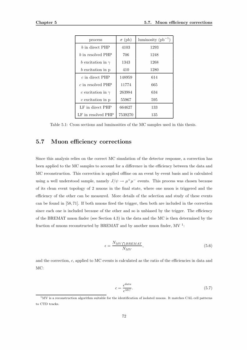
These samples were combined according to the cross sections given by Pythia and shown in Table

5.1. The contributions of processes where a b quark is extracted from the proton or photon to

the total bb cross section is about 27%. The parton density CTEQ5L [67] was used for the proton

and GRVG-LO [68] for the photon; the b-quark mass was set to 4.75 GeV and the b-quark string

fragmentation was performed according to the Peterson function with ǫ = 0.0041 [69]. The beauty

quarks were not forced to decay into muons and so the fraction of b decays into muons was given by

the branching fraction implemented in the generation according to the value given by the Particle

Data Group [70].

5.6.2 Charm event simulation

The production processes of charm are the same as for beauty and so equivalent samples were

generated. Again, the samples were combined according to the cross sections given by Pythia

and shown in Table 5.1. The c quark mass was set to 1.35 GeV and the events were required to

contain 2 jets each with:

• EjT ≥ 4 GeV

• |ηj | < 3

5.6.3 Light flavour event simulation

Due to the low mass of the quarks, production of light flavour (LF) events is dominated by resolved

photoproduction. In this sample, direct and resolved photoproduction processes were generated.

As with the charm sample, the events contained 2 jets with the same EjT and |ηj | requirements

and the generation cross sections are shown in Table 5.1. Events containing b and c quarks were

removed from the sample.

71

Chapter 5 5.7. Muon efficiency corrections

process σ (pb) luminosity (pb−1)

b in direct PHP 4103 1293

b in resolved PHP 706 1248

b excitation in γ 1343 1268

b excitation in p 410 1280

c in direct PHP 148959 614

c in resolved PHP 11774 665

c excitation in γ 263984 634

c excitation in p 55967 595

LF in direct PHP 664627 133

LF in resolved PHP 7539270 135

Table 5.1: Cross sections and luminosities of the MC samples used in this thesis.

5.7 Muon efficiency corrections

Since this analysis relies on the correct MC simulation of the detector response, a correction has

been applied to the MC samples to account for a difference in the efficiency between the data and

MC reconstruction. This correction is applied offline on an event by event basis and is calculated

using a well understood sample, namely J/ψ → µ+µ− events. This process was chosen because

of its clean event topology of 2 muons in the final state, where one muon is triggered and the

efficiency of the other can be measured. More details of the selection and study of these events

can be found in [58, 71]. If both muons fired the trigger, then both are included in the correction

since each one is included because of the other and so is unbiased by the trigger. The efficiency

of the BREMAT muon finder (see Section 4.3) in the data and the MC is then determined by the

fraction of muons reconstructed by BREMAT and by another muon finder, MV 1:

ǫ =NMV

T

BREMAT

NMV

, (5.6)

and the correction, c, applied to MC events is calculated as the ratio of the efficiencies in data and

MC:

c =ǫdata

ǫMC. (5.7)

1MV is a reconstruction algorithm suitable for the identification of isolated muons. It matches CAL cell patterns

to CTD tracks.

72

5.8. Control distributions Chapter 5

These corrections were calculated in bins of pµT and ηµ by the ZEUS collaboration muon group

and were provided as factors which were then applied in this analysis, also in bins of pµT and ηµ.

The dependence of the correction factors on these variables is largely due to geometrical effects of

the detector.

5.8 Control distributions

Figure 5.3 shows the distributions of the kinematic variables pµT and ηµ as well as those for the

jet associated with the muon pµ-jT and ηµ-j . Also shown is the distribution of xjj

γ . The data are

compared in shape to the MC simulations in which the relative contributions of beauty, charm and

LF were mixed according to the fractions measured in this analysis as described in Chapter 6. The

comparison shows that the data are generally well described by the MC. In the ηµ distribution,

and correspondingly in the ηµ-j distribution, an apparent shift of the data to larger η with respect

to the MC can be seen.

73

Chapter 5 5.8. Control distributions

ZEUS

(GeV)µT

p0 2 4 6 8 10 12 14

muo

ns

1

10

210

310 (a)

µη−2 −1.5 −1 −0.5 0 0.5 1 1.5 2

muo

ns

200

400

600

800

1000

1200

(b)

(GeV)−jµT

p5 10 15 20 25 30 35 40

jets

1

10

210

310(c)

−jµη−2 −1.5 −1 −0.5 0 0.5 1 1.5 2

jets

200

400

600

800

1000

1200

(d)

jjγx

0 0.2 0.4 0.6 0.8 1

even

ts

0

1000

2000

3000

4000

5000

(e)−1ZEUS 126pb

+LF MCc+cbbLF MC

cc

bb

Figure 5.3: Distributions of (a) pµT , (b) ηµ, (c) pµ-j

T , (d) ηµ-j and (e) xjjγ . The data are compared

to a mixture of beauty (shaded histogram), charm (dotted line) and light flavour (dashed line)

Pythia MC predictions, combined according to the fractions given by the two-dimensional p relT -δ

fit. The total MC distribution is shown as the solid line. The kinematic region is restricted to

pµT > 1.5 GeV (pµ

T > 2.5 GeV) for (a)((b)-(e)).

74

Chapter 6

Beauty quark identification

In the analysis presented here, events with at least two jets were selected and b quarks were iden-

tified through their semi-leptonic decay into muons. The branching ratio for this decay channel is

acceptably large (∼ 10%) and the muon provided a clean signature since it is minimally ionising and

could traverse the inner detector components to reach the muon chambers, whereas other particles

were stopped before the muon detection system. Thus, in this analysis, beauty in photoproduction

has been studied in the following decay chain:

ep→ ebbX → ejjµX (6.1)

The major backgrounds to this process were cc production and processes in which final state

hadrons were wrongly identified as muons. The mechanism for cc production in ep collisions is

essentially the same as for bb production and the semi-leptonic decay of charm to muons also has

a branching ratio of ∼ 10%. Since the cc production cross section was much higher at HERA

than that of bb production and the final state topologies of the two were very similar, this process

represented an important background in this analysis. Another possible background was due to the

misidentification of hadrons, such as pions or kaons, as muons in the muon chambers. Although

these particles had a low probability of reaching the muon chambers, they were produced copiously

at HERA and so formed another large background component.

In this analysis the fraction of beauty quarks in the sample is extracted using a statistical method,

exploiting both the large mass of the b quark and the long lifetime of the B hadron to separate

signal and background.

75

Chapter 6 6.1. The p relT method

6.1 The prelT method

Figure 6.1: Illustration of the p relT variable.

The mass of the b quark is approximately 3 times the mass of the c quark. As a result, it is to

be expected that the decay products of the B hadron will have a harder transverse momentum

spectrum compared with the products of charm decay. In particular, muons from semi-leptonic

beauty decays tend to be produced with high transverse momentum with respect to the direction

of the mother B hadron,

p relT,true = |~p rel

T,true| = |~p µ × p had| =|~p µ × ~p had|

|~p had| , (6.2)

where ~p µ is the muon momentum vector, p had is the unit vector along the B-hadron direction

and ~p had is the B hadron momentum vector. Since B hadrons rapidly decay, their direction is

approximated by that of the jet associated with the muon, as shown in Fig. 6.1. The transverse

momentum of the muon relative to this associated jet (which includes the muon) is given by

p rel,incl.T =

|~p µ × ~p j ||~p j | , (6.3)

where ~p j is the momentum vector of the jet associated with the muon. An alternative definition

for p relT uses a slightly modified jet axis as a reference by subtracting the muon momentum from the

76

6.1. The p relT method Chapter 6

ZEUS

(GeV)relT

p0 1 2 3 4 5

muo

ns

1

10

210

310

(a)

−1ZEUS 126pb

+LF MCc+cbb

(cm)δ−0.08 −0.04 0 0.04 0.08

muo

ns

1

10

210

310

(b)

LF MC

MCcc

MCbb

Figure 6.2: Distributions of (a) p relT and (b) the muon impact parameter, δ. The data are com-

pared to a mixture of beauty (shaded histogram), charm (dotted line) and light flavour(dashed

line) Pythia MC samples. The total MC distribution is shown as the solid line. The relative

contributions of beauty, charm and light flavour were mixed according to the fractions measured

in this analysis as described in Sec.6.4.

jet momentum, thus shifting the p relT spectrum to larger values. Subtracting the muon momentum

enhances the discriminating power of the p relT variable, since a jet axis defined including the muon

would be correlated to the muon track’s momentum, and hence would diminish its discriminating

power. This is especially important in the case of low track multiplicity jets, in which the muon

has the possibility to strongly influence the definition of the jet axis. This definition is used in this

analysis and is given by

p relT =

|~p µ × (~p j − ~p µ)||~p j − ~p µ| . (6.4)

Figure 6.2(b) shows the distribution of p relT for the data and the signal (bb) and background (cc,

LF) MC samples. The p relT spectrum for beauty events is harder than for charm or light flavour

events and it is this difference which enables a separation of signal and background.

77

Chapter 6 6.2. The impact parameter method

jetjet

µ

µ µ

δ < 0

δ > 0

δ

beamposition

beamposition

beamposition

Figure 6.3: Illustration of the signed impact parameter.

6.2 The impact parameter method

The long lifetime of beauty and char m hadrons means that the products of beauty and charm

decays are produced at a secondary vertex some distance, L, from the production of the hadron.

With very precise position measurements of the decay products, their tracks can be unambiguously

associated to the secondary vertex. However, requiring this level of precision leads to a significant

loss of signal candidate events. A statistical extraction of the heavy flavour content of a larger

sample can be achieved using a variable related to L. The impact parameter, δ, of a particle

coming from a hadron decay is defined as the closest distance, in the r-φ plane, between the path

of the particle’s trajectory and the production vertex of the hadron and is given by

δtrue = LT sinα, (6.5)

where LT = L sin θ, θ being the polar angle of the decaying hadron, and α is the angle in the r-φ

plane between the hadron direction and the direction of the decay product. Experimentally, in

semi-leptonic decays producing muons, the impact parameter is the distance of closest approach of

the reconstructed muon track to the event primary vertex, given by the beam spot. The direction

of the hadron trajectory is approximated by the direction of the axis of the jet associated with the

muon.

In semi-leptonic charm and beauty decays, the impact parameter is expected to be a positive non-

zero quantity. Therefore this variable can be used to discriminate between heavy flavour events

and events involving lighter quarks, for which we would expect an impact parameter of zero.

Introducing a sign to the impact parameter allows a statistical separation of detector resolution

effects from the effects of the lifetime of a heavy hadron. The sign of δ is positive if the muon

intercepts the axis of the associated jet within the jet hemisphere, otherwise δ is negative, as

78

6.3. Comparison between data and MC Chapter 6

shown in Fig. 6.3. A negative δ is an unphysical scenario due to the resolution of the detector.

As such, muon tracks originating at the event primary vertex, as in light flavour events, will

have a δ spectrum symmetric about zero the width of which reflects the finite track and vertex

reconstruction resolution. Decays of beauty and charm hadrons are characterised by the excess

seen in the positive δ spectrum. The difference in lifetime between beauty and charm hadrons

leads to a significant difference in the δ spectra of the muons in charm and beauty events with

beauty events having a harder δ distribution. Figure 6.2(b) shows the muon impact parameter

distributions of the data, bb, cc and LF MC samples. The characteristic asymmetric δ distributions

of the beauty MC and to a lesser extent, of the charm MC can be clearly seen.

6.3 Comparison between data and MC

Since the beauty content of the data sample is extracted statistically in this method using distri-

butions predicted by the Monte Carlo, it is essential that the discriminating variables, p relT and δ

are well reproduced by the Monte Carlo description. In this section, the corrections made to these

variables are described.

6.3.1 prelT correction

In-flight decays of pions and kaons form the largest source of muon candidates in the light flavour

background. The p relT distribution of the muon background fbkg

µ (p relT ) can be expressed as:

fbkgµ (p rel

T ) = fbkgx (p rel

T )Px→µ(p relT ), (6.6)

where fbkgx (p rel

T ) is the p relT distribution of unidentified particle x and Px→µ(p rel

T ) is the probability

that an unidentified particle is identified as a muon. This probability can be determined from

Monte Carlo as

Px→µ(p relT ) =

fMC,bkgµ (p rel

T )

fMC,bkgx (p rel

T ), (6.7)

where fMC,bkgµ (p rel

T ) and fMC,bkgx (p rel

T ) are the Monte Carlo muon and unidentified track p relT

distributions. Therefore, the p relT distribution of the muon background can be expressed as a

correction to the muon distribution obtained from Monte Carlo:

79

Chapter 6 6.3. Comparison between data and MC

fbkgµ (p rel

T ) = fMC,bkgµ (p rel

T )fbkg

x (p relT )

fMC,bkgx (p rel

T ). (6.8)

This is known as the p relT correction. The distribution fbkg

x (p relT ) can be obtained from a data

sample of dijet events without the requirement of a muon since the beauty contribution in such a

sample is very small (2%), i.e.

fbkgx (p rel

T ) ≃ fx(p relT ). (6.9)

This inclusive dijet sample was selected using the same cuts as in the analysis, see Section 5.5, but

without the requirement of a muon in the event. Instead, the correction was calculated using all

tracks in the event which pass the following quality cuts:

• pT > 2.5 GeV (pT > 1.5 GeV for the p relT correction applied to the pµ

T cross section);

• −1.6 < η < 2.3;

• The track is associated with a jet by the requirement that ∆R(track− jet) < 1.0 where

∆R(track− jet) =√

(ηtrack − ηjet)2 + (φtrack − φjet)

2;

The p relT value was then calculated for each track. Figure 6.4(a) shows the p rel

T spectrum for the

data and MC, normalised to the data. The MC has a more rapid fall off to higher value of p relT

than the data. The correction factorfx(p rel

T )

fMCx (p rel

T)

is shown in Fig 6.4(b) given by the ratio of the data

and MC distributions in Fig. 6.4(a). These p relT correction factors are calculated for each bin of

each cross section measured in this analysis and applied as such to the light flavour MC sample.

Since the charm background is composed not only of a fake muon contribution but also includes

muon final states from charm decays, it would not be appropriate to apply the same correction to

the charm sample as for the light flavour sample. On the other hand, since it is not possible to

extract the p relT distribution of charm from the data, such correction factors cannot be calculated

directly for charm background. Therefore, as an estimation, 50% of the correction factor applied

to the light flavour MC sample was applied to the charm MC sample.

6.3.2 Impact parameter smearing

Using the same inclusive dijet sample as in Section 6.3.1 and plotting the impact parameter dis-

tribution for tracks, as in Fig. 6.5, a discrepancy between MC and data is observed. The width of

80

6.3. Comparison between data and MC Chapter 6

(GeV)relT

p0 1 2 3 4 5

Ent

ries

410

510

Data

MC

(a)

(GeV)relT

p0 1 2 3 4 5

data

/MC

0.95

1

1.05

1.1

1.15

1.2

1.25

1.3

(b)

Figure 6.4: (a) p relT distribution for inclusive dijet samples of data and PYTHIA MC events

(normalised to the data). (b) The ratio of data to MC events as a function of p relT .

the δ distribution in the MC is smaller than that of the data. The reasons for this disagreement

are related to the following:

• insuffcient accuracy of the dead material simulation;

• intrinsic hit and track resolution overestimating the real tracking detector resolution;

• incomplete version of the alignment of the MVD implemented for this analysis.

A correction can be calculated on the same inclusive data sample so as to reduce the dependence

of the correction on Monte Carlo. A full description of the method employed to calculate this

correction can be found in [2]. The correction, which was calculated by fitting the data with a

double convolution of a Gaussian and a Breit-Wigner distribution, takes the form:

∆δ = NBW(e(a−b·pµ

T) + c) · d+NGauss(f + g · pµ

T ), (6.10)

where NBW and NGauss are random numbers which are distributed according to a Breit-Wigner

and Gaussian function respectively, both with unit width, and a, b, c, d, f, and g are constants.

The correction, which depends on pµT , is applied to each MC event in the beauty, charm and light

flavour samples in the analysis. Figure 6.6 shows the δ distributions of the inclusive data and MC

samples after the application of the correction. The MC description of the data is much improved.

81

Chapter 6 6.3. Comparison between data and MC

δ (cm)

Ent

ries

+ dataMC

δ (cm)

Ent

ries

δ (cm)

Ent

ries

δ (cm)

Ent

ries

δ (cm)

Ent

ries

δ (cm)

Ent

ries

δ (cm)

Ent

ries

δ (cm)

Ent

ries

δ (cm)

Ent

ries

10 3

10 4

10 5

-0.15 -0.05 0.05 0.15

10 3

10 4

-0.15 -0.05 0.05 0.15

10 3

10 4

10 5

-0.15 -0.05 0.05 0.15

10 2

10 3

10 4

-0.15 -0.05 0.05 0.15

10 2

10 3

10 4

-0.15 -0.05 0.05 0.15

10 2

10 3

10 4

-0.15 -0.05 0.05 0.15

10 2

10 3

10 4

-0.15 -0.05 0.05 0.1510

10 2

10 3

10 4

-0.15 -0.05 0.05 0.15

10 2

10 3

10 4

-0.15 -0.05 0.05 0.15

(0.5 - 1.0) (1.0 - 1.5) (1.5 - 2.0)

(2.0 - 2.5) (2.5 - 3.0) (3.0 - 3.5)

(3.5 - 4.0) (4.0 - 4.5) (4.5 - 5.0)

Figure 6.5: MC impact parameter distributions (blue histograms) compared to the data (black

points) in bins of pT (the bin range range for each plot in GeV is given in the brackets). [2, 3] .

10 3

10 4

10 5

-0.15 -0.05 0.05 0.15

10 3

10 4

10 5

-0.15 -0.05 0.05 0.1510 2

10 3

10 4

-0.15 -0.05 0.05 0.15

10 2

10 3

10 4

-0.15 -0.05 0.05 0.15

10 2

10 3

10 4

-0.15 -0.05 0.05 0.15

10 2

10 3

10 4

-0.15 -0.05 0.05 0.15

10 2

10 3

10 4

-0.15 -0.05 0.05 0.15

10

10 2

10 3

10 4

-0.15 -0.05 0.05 0.15

IDEntriesMeanRMS

1301 619235 0.1082E-02 0.3635E-01

δ (cm)

Ent

ries + data

MC

IDEntriesMeanRMS

1302 304429 0.1037E-02 0.2914E-01

δ (cm)

Ent

ries

IDEntriesMeanRMS

1303 164429 0.9689E-03 0.2624E-01

δ (cm)

Ent

ries

IDEntriesMeanRMS

1304 93578 0.8862E-03 0.2447E-01

δ (cm)

Ent

ries

IDEntriesMeanRMS

1305 104652 0.7401E-03 0.2241E-01

δ (cm)

Ent

ries

IDEntriesMeanRMS

1306 64681 0.6210E-03 0.2186E-01

δ (cm)

Ent

ries

IDEntriesMeanRMS

1307 41119 0.6683E-03 0.2124E-01

δ (cm)

Ent

ries

IDEntriesMeanRMS

1308 26300 0.4407E-03 0.2084E-01

δ (cm)

Ent

ries

IDEntriesMeanRMS

1309 17813 0.6102E-03 0.2079E-01

δ (cm)

Ent

ries

10

10 2

10 3

10 4

-0.15 -0.05 0.05 0.15

(0.5 - 1.0) (1.0 - 1.5) (1.5 - 2.0)

(2.0 - 2.5) (2.5 - 3.0) (3.0 - 3.5)

(3.5 - 4.0) (4.0 - 4.5) (4.5 - 5.0)

Figure 6.6: MC impact parameter distributions (blue histograms), after the application of smearing

correction, compared to the data (black points) in bins of pT (the bin range range for each plot in

GeV is given in the brackets). [2, 3]. 82

6.4. Extraction of the beauty fraction Chapter 6

0 5 10 15 20 25 30

even

ts

1

10

210

310

0 5 10 15 20 25 301

10

210

310

1

10

210

3102005 Data

bb MC

cc MC

lf MC

bb+cc+lf MC

-0.08 -0.025 -0.01 0 0.01 0.025 0.08

rel.T

p(GeV)

δ(cm)

0. 5. 0. 5. 0. 5. 0. 5. 0. 5. 0. 5.

Figure 6.7: Fit of MC distributions to a data distribution of p relT in bins of δ.

6.4 Extraction of the beauty fraction

The beauty component of the data sample was determined using the differences in the shapes of

distributions of p relT and δ for signal and background processes. These distributions were provided

by MC simulation and by performing a fit to the data distribution, the fraction of beauty events in

the sample was extracted. In order to combine the discriminating properties of the two variables,

the fit was made to a two-dimensional distribution of p relT in bins of δ, as shown in Fig. 6.7. The

fit f was a three component fit:

f = abbfbb + accf

cc + (1 − abb − acc)fLF , (6.11)

using the MC predicted shapes for beauty (f bb), charm (f cc) and light flavour (fLF ) events. Thus

the fractions of beauty (abb) and charm (acc) events were extracted. The fit to the data distribution,

fdata, used the mimimum-χ2 method, in which the χ2 value:

χ2 =

nbins∑

i

(fdatai − fi)

2

σ2i,data + (abbσi,bb)

2 + (accσi,cc)2 + ((1 − abb − acc)σi,LF )2(6.12)

is calculated iteratively for different values of abb and acc until the minimum is found. The denom-

inator takes into account the statistical uncertainties of the beauty (σbb), charm (σcc) and light

flavour (σLF ) samples. The fit was repeated in each bin of every cross section. The results of the

global fit to complete data sample (pµT > 2.5 GeV) are given below.

• abb = 0.150±0.0140.013

83

Chapter 6 6.4. Extraction of the beauty fraction

ZEUS

0

0.1

0.2

0.3

0.4

0.5

0.6

0.7

0.8

0.9

1

0 0.1 0.2 0.3 0.4 0.5 0.6 0.7 0.8 0.9 1

ZEUS

0

0.1

0.2

0.3

0.4

0.5

0.6

0.7

0.8

0.9

1

0 0.1 0.2 0.3 0.4 0.5 0.6 0.7 0.8 0.9 1

b fraction

c fr

actio

n

b fraction

c fr

actio

n

b fraction

c fr

actio

n ZEUS 126 pb -1

68% prob. contours

physical region

unphysical region

pT rel vs δ

δ

pT rel

Figure 6.8: Contours of 68% probability in the plane defined by the beauty and charm fractions.

The results of the χ2 fit to the two-dimensional p relT -δ distribution and to the p rel

T and δ-only

distributions are shown. The diagonal line shows the boundary of the physical region in which the

fractions of b, c and LF are positive.

• acc = 0.398±0.0500.050

• aLF = 1 − abb − acc = 0.452±0.0490.052

Figure 6.8 shows the 68% probability contours from the fit described above and also from the

the fits carried out using p relT or δ alone. It shows that the two variables give complementary

information. The p relT fit alone is able to distinguish between beauty and the background of charm

and LF. It is not able to separate these two backgrounds. On the other hand, the δ fit gives a

good determination of the heavy quark content. Using the combination of the two gives a vastly

improved result.

84

Chapter 7

Cross-section measurement

A study of beauty photoproduction in dijet events has been carried out with 126 pb−1 of data

collected using the ZEUS detector in 2005 [1]. Due to their large mass, the production of b quarks

in ep collisions should be accurately calculable in perturbative QCD. Therefore it is interesting

to compare such predictions to experimental results. In this chapter, measurements of the total

cross section σ(ep→ ebbX → ejjµX ′) and differential cross sections as a function of muon and jet

variables are presented for beauty production. They are compared to NLO QCD predictions and

and Monte Carlo models.

The dijet sample of beauty photoproduction events was also used to study higher-order QCD

topologies. At LO, the two jets in the event are produced back-to-back in azimuthal angle, such

that ∆φjj = φj1 − φj2 = π. Additional soft radiation causes small azimuthal decorrelations,

whilst ∆φjj significantly lower than π is evidence of additional hard radiation. In this chapter, the

differential cross section with respect to ∆φjj is also presented for beauty photoproduction and

again compared to NLO QCD predictions and Monte Carlo models.

The total and differential visible cross sections were measured for final states with at least one

muon and two jets in the following kinematic region:

• Q2 < 1 GeV2 and 0.2 < y < 0.8;

• pj1,j2T > 7, 6 GeV and |ηj1,j2| < 2.5;

• pµT > 2.5 GeV (pµ

T > 1.5 GeV for dσ/dpµT ) and −1.6 < ηµ < 1.3;

• at least one muon is associated with a jet with pjT > 6 GeV.

85

Chapter 7 7.1. Purities, efficiencies and acceptance corrections

(GeV)µT

p2 3 4 5 6 7 8 9 10

Pur

ity

0

0.1

0.2

0.3

0.4

0.5

0.6

0.7

0.8

0.9

1

(GeV)µT

p2 3 4 5 6 7 8 9 10

Effi

cien

cy

0

0.1

0.2

0.3

0.4

0.5

0.6

0.7

0.8

0.9

1

(GeV)µT

p2 3 4 5 6 7 8 9 10

Acc

epta

nce

0

0.1

0.2

0.3

0.4

0.5

0.6

0.7

0.8

0.9

1

Figure 7.1: Purity, p, efficiency, ǫ and acceptance correction factor, A, for the differential cross

section as a function of pµT .

The visible cross section was determined using:

σ(ep→ ebbX → ejjµX ′) =abbNµ

A · L , (7.1)

where abb is the fraction of beauty events in the sample, extracted statistically as described in Sec-

tion 6.4, Nµ is the number of muon candidates selected from a data set with integrated luminosity

L. The acceptance correction, A, which takes into account migration of events from bin to bin and

the reconstruction inefficiency is described in Section 7.1.

A visible differential cross section with respect to a variable Y is given by a corresponding formula,

dσ

dY=

abb(i)Nµ(i)

A(i) · L · ∆Yi

, (7.2)

where abb(i), Nµ(i) and A(i) are the beauty fraction, number of muon candidates and acceptance

correction respectively in a given bin, i, of width ∆Yi.

7.1 Purities, efficiencies and acceptance corrections

In order to obtain a cross section from detector level quantities, the purity, efficiency and acceptance

correction were calculated in each bin using Pythia MC. The purity, p(i), and efficiency, ǫ(i), are

given by,

86

7.2. Determination of the systematic uncertainties Chapter 7

p(i) =Nrec∩gen(i)

Nrec(i), (7.3)

ǫ(i) =Nrec∩gen(i)

Ngen(i), (7.4)

where Nrec(i) is the number of reconstructed events and Ngen(i) is the number of events generated

in bin i which pass the kinematic cuts. Nrec∩gen(i) is the number of events which are generated

and reconstructed in the same bin, i. The purity can therefore be interpreted as the fraction of

reconstructed events in a certain bin which were originally generated in that bin. Similarly, the

efficiency can be interpreted as the fraction of generated events which were then reconstructed in

the same bin. The acceptance correction, A(i), can be calculated from the purity and efficiency

as,

A(i) =ǫ(i)

p(i). (7.5)

The purity, efficiency and acceptance correction as functions of pµT are shown in Fig. 7.1. For

all other variables, these figures are included in Appendix A. The efficiency includes the muon

efficiency corrections and so low values can be attributed in part to the inefficiency in muon

reconstruction.

7.2 Determination of the systematic uncertainties

The following sources of systematic uncertainty were considered. The resulting uncertainty on

the total cross section is given in parentheses and the uncertainties on the differential cross sec-

tions are given in Appendix B. The total systematic uncertainty is determined by summing these

contributions in quadrature.

Muon acceptance

The uncertainty on the muon acceptance, including the efficiency of the muon chambers, of the

reconstruction and of the B/RMUON matching to central tracks has been determined in a study

based on a dimuon sample, as described in Section 5.7. The efficiency of the muon trigger in the

MC was corrected so that it reproduced the efficiency as measured in the data, as described in

Section 5.1.1. The size of the correction was varied within its uncertainties. These variations were

carried out simultaneously (±7%).

87

Chapter 7 7.2. Determination of the systematic uncertainties

µη-2 -1.5 -1 -0.5 0 0.5 1 1.5 2

data

/MC

0

0.2

0.4

0.6

0.8

1

1.2

1.4

1.6

1.8

2

(a)

µη-2 -1.5 -1 -0.5 0 0.5 1 1.5 2

muo

ns

20

40

60

80

100

120

140

160

180

200-1ZEUS 126pb

+LF MCc+cbb(b)

Figure 7.2: (a) The factors used to reweight the MC taken from the ratio of the numbers of data

and MC events in bins of ηµ. (b) Comparison of ηµ control distribution for data and MC for

beauty-enriched samples obtained by the requirement of p relT > 2 GeV

Energy scale

The absolute energy scale of the calorimeter is known to be reproduced by the MC to within ±3%.

Therefore the error due to the uncertainty of the energy scale was evaluated by varying the energy

of the jets and the inelasticity yJB in the MC by ±3% (±4%).

MVD efficiency

The efficiency of finding a track with 4 MVD hits in an inclusive sample of CTD tracks (pT >

2.5 GeV, 0.55 < θ < 2.75) was measured in the data and in the MC. The ratio of the measured

efficiencies was found to be 0.94 and was applied as a correction to the acceptance. The uncertainty

on this ratio was included as a systematic uncertainty (±3%).

Dijet trigger efficiency

The efficiency of the dijet trigger in the MC was corrected so that it reproduced the efficiency as

measured in the data, as described in Section 5.1.1. The systematic uncertainty on the size of this

correction was negligible.

ηµ MC description

The data ηµ distribution was not well described by the MC simulation. As shown in Fig. 5.3(b),

the MC distribution is shifted to lower values of ηµ with respect to the data. As a systematic

88

7.2. Determination of the systematic uncertainties Chapter 7

check, MC events were weighted, in order to account for these differences, by factors taken from

the ratio of the data and MC in each bin of the ηµ distribution. Each MC event was given the

weight corresponding to the bin containing the highest-pT muon in the event. The factors are

shown in Fig. 7.2(a). The discrepancy in ηµ control distribution was also present in a signal

enhanced sample (using the requirement p relT > 2 GeV), as shown in Fig. 7.2(b), and therefore the

reweighting was applied to both signal and background MC samples. The resulting variation in

the cross section was found to be largest in dσdηµ and dσ

dηµ−j , however the effect on the total cross

section was negligible (< 1%).

Impact parameter correction

The uncertainty on the size of the correction to the shape of the impact parameter distribution

for the MC samples, as described in Section 6.3.2, was evaluated by varying the widths of the

Gaussian and Breit-Wigner distributions used in the correction function by +20% and −10% of

their nominal values. These variations are such that the global MC distribution still provides a

good description of the data (+6%−10%).

prelT correction

The uncertainty on the p relT shape of the LF and charm background was evaluated by:

• varying the correction applied to the LF background by ±20% of its nominal value (±2%).

• varying the p relT shape of the charm component by removing or doubling the correction

applied (±4%).

Physics process contributions in MC

The contributions of processes to the overall MC samples are combined according to the corre-

sponding production cross sections taken from the Pythia MC prediction. The uncertainty on

these MC model cross sections is estimated in the following way.

The contribution of processes in which a b quark comes from the proton or photon in Pythia was

varied by +100%/ − 50% and simultaneously the contribution of gg → bb, qq → bb events was

varied by − 50%/+ 100%. Figure 7.3(a) shows the change in shape of the MC distribution of dσ

dxjjγ

when these variations are made (±4%).

The contribution of γg → bb processes in Pythia was decreased by 20% and all other processes

were increased by +100%. The change in shape of the dσ

dxjjγ

MC distribution is shown in Fig. 7.3(b)

(±2%).

89

Chapter 7 7.3. Theoretical predictions

jjγx

0 0.2 0.4 0.6 0.8 1

(pb

)jj γ

/ dx

σd

1

10

2102005 Data

PYTHIA MC

PYTHIA MC: fl.exc.-50%

PYTHIA MC: fl.exc.+100%

jjγx

0 0.2 0.4 0.6 0.8 1

(pb

)jj γ

/ dx

σd

1

10

210

(a)

jjγx

0 0.2 0.4 0.6 0.8 1

(pb

)jj γ

/ dx

σd

1

10

210

(b)

2005 Data

PYTHIA MC

PYTHIA MC: dir.-20%

jjγx

0 0.2 0.4 0.6 0.8 1

(pb

)jj γ

/ dx

σd

1

10

210

Figure 7.3: dσ

dxjjγ

for data and nominal Pythia MC samples. Also shown are dσ

dxjjγ

for Pythia MC

samples in which (a) the contribution of flavour-excitation events was varied by +100%/ − 50%

and simultaneously the contribution of gg → bb, qq → bb events was varied by − 50%/ + 100%

and (b) the contribution of γg → bb processes was decreased by 20% and all other processes were

increased by +100%

The size of these variations were such that the comparison between MC and data for dσ

dxjj

dγ

was still

satisfactory (see Fig. 7.3).

7.3 Theoretical predictions

The measured cross sections are compared to NLO QCD predictions based on the FMNR [19]

program. The parton distribution functions used for the nominal prediction were GRVG-HO

[68] for the photon and CTEQ5M [67] for the proton. The b-quark mass was set to mb =

4.75 GeV, and the renormalisation and factorisation scales to the transverse mass, µr = µf =

mT =

√

12

(

(pbT )2 + (pb

T )2)

+m2b , where p

b(b)T is the transverse momentum of the b (b) quark in the

laboratory frame. Jets were reconstructed by running the kT algorithm on the four-momenta of

the b and b quarks and of the third light parton (if present) generated by the program. The frag-

mentation of the b quark into a B hadron was simulated by rescaling the quark three-momentum

(in the frame in which pbZ = −pb

Z , obtained with a boost along Z) according to the Peterson [69]

fragmentation function with ǫ = 0.0035. The muon momentum was generated isotropically in the

B hadron rest frame from the decay spectrum given by Pythia which is in good agreement with

measurements made at B factories [72].

90

7.4. Total cross section Chapter 7

The NLO cross sections, calculated for jets made of partons, were corrected for jet hadronisation

effects to allow a direct comparison with the measured hadron-level cross sections. The correction

factors, Chad, were derived from the MC simulation as the ratio of the hadron-level to the parton-

level MC cross sections. The parton level is defined as being the result of the parton-showering stage

of the simulation and the hadron level is defined as the point after hadronisation (see Fig. 2.2).

Therefore the factors, Chad, can be used to correct theoretical predictions, which have partons as

the final state, to the hadron level so that they can be compared with the measured cross sections.

The corrections were found to be typically small, with a maximum value of ∼ 20%, and did not

change the shapes of the cross section distributions. Values of Chad for each bin of each cross

section are given in Tables 7.1, 7.2, 7.3 and 7.4.

To evaluate the uncertainty on the NLO calculations, the b-quark mass and the renormalisation and

factorisation scales were varied simultaneously to maximise the change, from mb = 4.5 GeV and

µr =µf = mT /2 to mb = 5.0 GeV and µr =µf = 2mT , producing a variation in the cross section

from +34% to −22%. The effect on the cross section of a variation of the Peterson parameter ǫ and

of a change of the fragmentation function from the Peterson to the Kartvelishvili parameterisation

was found in a previous publication [21] to be of the order of 3%. The effects of using different

sets of parton densities and of a variation of the strong coupling constant were found to be within

±4%. These effects are negligible with respect to that of a variation of the b-quark mass and the

renormalisation and factorisation scales and are therefore not included. The uncertainty due to the

hadronisation correction was also found to be negligible with respect to the dominant uncertainty.

7.4 Total cross section

The total visible cross section is

σ(ep → ebbX → ejjµX ′) = 38.6 ± 3.5(stat.)+4.6−4.9(syst.) pb. (7.6)

This result is compared to the NLO QCD calculation described in Section 7.3. The prediction for

the total visible cross section is

σ(ep→ ebbX → ejjµX ′) = 39.2+14.4−6.9 pb, (7.7)

in excellent agreement with the data.

91

Chapter 7 7.5. Muon variable differential cross sections

7.5 Muon variable differential cross sections

Figure 7.4 and Tables 7.1 and 7.2 show the visible differential cross sections as a function of

pµT , ηµ, pµ−j

T and ηµ−j . The visible cross section as a function of pµT is measured in the range

pµT > 1.5 GeV, extending the kinematic region to lower pµ

T than in the previous ZEUS and H1

measurements [21, 22], while the other cross sections are measured for pµT > 2.5 GeV. The NLO

QCD predictions describe the data well and the Pythia MC also gives a good description of the

shapes.

The visible differential cross section as a function of ηµ is also compared with the previous ZEUS

measurement [21], which used the p relT method to extract the beauty fraction. The two measure-

ments agree well. The measurement presented by H1 [22] refers to a slightly different definition of

the cross section and therefore cannot be compared to directly. However a qualitative comparison

does not confirm their observation of an excess at low pµT .

7.6 Dijet differential cross sections

Figure 7.5(a) and Table 7.3 show the visible dijet cross section as a function of xjjγ (Equation 2.11).

The xjjγ variable corresponds at LO to the fraction of the exchanged-photon momentum entering

the hard scattering process. In photoproduction, events can be classified into two types of process

in LO QCD: direct and resolved processes, as described in Section 1.6. The xjjγ variable provides

a tool to measure the relative importance of direct processes, which gives a peak at xjjγ ∼ 1, and

of resolved processes, which are distributed over the whole xjjγ range. The measurement presented

here shows that the dominant contribution to the visible cross section comes from the high-xjjγ

peak but a low-xjjγ component is also apparent. The NLO QCD prediction describes the measured

visible cross section well. Pythia also gives a good description of the shape of the distribution.

Dijet angular correlations are particularly sensitive to higher-order effects and are therefore suitable

to test the limitations of fixed-order perturbative QCD calculations. At LO, the differential cross

section as a function of ∆φjj is a delta function peaked at π. At NLO, exclusive three-jet production

populates the region 23π < ∆φjj < π, whilst smaller values of ∆φjj require additional radiation

such as a fourth jet in the event. However, it should be noted that an NLO QCD calculation can

produce values of ∆φjj < 23π when the highest-pT jet is not in the accepted kinematic region.

The visible differential cross section as a function of ∆φjj is shown in Fig. 7.5(b) and Table 7.4.

The NLO QCD predictions describe the data well. Visible cross sections as a function of ∆φjj have

92

7.6. Dijet differential cross sections Chapter 7

ZEUS

(GeV)µT

p2 3 4 5 6 7 8 9 10

(pb

/GeV

)µ T

/ dp

σd

1

10

(a)

-1ZEUS 126pb

had⊗NLO QCD

PYTHIA MC x 1.3

(GeV)µT

p2 3 4 5 6 7 8 9 10

(pb

/GeV

)µ T

/ dp

σd

1

10

-1ZEUS 126pb

had⊗NLO QCD

PYTHIA MC x 1.3

µη-1.5 -1 -0.5 0 0.5 1

(pb

)µ η

/ d

σd

0

5

10

15

20

25

30

(b)

µη-1.5 -1 -0.5 0 0.5 1

(pb

)µ η

/ d

σd

0

5

10

15

20

25

30 -1ZEUS 96-00 110pb

(GeV)-jµT

p10 15 20 25 30

(pb

/GeV

)-jµ T

/dp

σd

-110

1

10

(c)

(GeV)-jµT

p10 15 20 25 30

(pb

/GeV

)-jµ T

/dp

σd

-110

1

10

-jµη-1.5 -1 -0.5 0 0.5 1

(pb

)-jµ η

/dσd

0

5

10

15

20

25

30

-jµη-1.5 -1 -0.5 0 0.5 1

(pb

)-jµ η

/dσd

0

5

10

15

20

25

30

(d)

Figure 7.4: Differential cross section as a function (a) pµT , (b) ηµ, (c) pµ−j

T and (d) ηµ−j for

Q2 < 1 GeV2, 0.2 < y < 0.8, pj1,j2T > 7, 6 GeV, |ηj1,j2 | < 2.5, and −1.6 < ηµ < 1.3. For the pµ

T

cross section, the kinematic region is defined as pµT > 1.5 GeV and as pµ

T > 2.5 GeV for all other

cross sections. The filled circles show the results from this analysis and the open circles show the

results from the previous ZEUS measurement. The inner error bars are statistical uncertainties

while the external bars show the statistical and systematic uncertainties added in quadrature. The

band represents the NLO QCD predictions with their uncertainties. The Pythia MC predictions

are also shown (dashed line).

93

Chapter 7 7.6. Dijet differential cross sections

pµT range dσ/dpµ

T ± stat.± syst. Chad

(GeV) (pb/GeV)

1.5, 2.5

2.5, 4.0

4.0, 6.0

6.0, 10.0

41.05 ± 7.74+8.26−8.51

15.78 ± 1.96+2.03−1.98

4.87 ± 1.03+0.69−0.67

0.84 ± 0.27+0.11−0.11

0.87

0.93

0.98

1.01

ηµ range dσ/dηµ ± stat.± syst. Chad

(pb)

−1.60,−0.75

−0.75, 0.25

0.25, 1.30

3.86 ± 1.37+1.40−0.92

16.81 ± 2.30+2.34−2.15

19.70 ± 2.43+2.43−3.09

0.83

0.89

0.92

Table 7.1: Differential muon cross section as a function of pµT and ηµ. For further details see text.

The multiplicative hadronisation correction, Chad, applied to the NLO prediction is shown in the

last column.

pµ-jT range dσ/dpµ-j

T ± stat.± syst. Chad

(GeV) (pb/GeV)

6, 11

11, 16

16, 30

4.74 ± 0.57+0.60−0.59

1.78 ± 0.32+0.24−0.22

0.33 ± 0.10+0.05−0.05

0.89

0.89

0.92

ηµ-j range dσ/dηµ-j ± stat.± syst. Chad

(pb)

−1.6,−0.6

−0.6, 0.4

0.4, 1.4

6.13 ± 1.41+1.50−0.82

13.89 ± 2.20+2.08−2.21

16.42 ± 2.29+1.70−2.29

0.77

0.84

0.99

Table 7.2: Differential cross section for jets associated with a muon as a function of pµ-jT and ηµ-j .

For further details see text.

94


ZEUS

jjγx

0 0.2 0.4 0.6 0.8 1

(pb

)jj γ

/ dx

σd

1

10

210(a)

jjγx

0 0.2 0.4 0.6 0.8 1

(pb

)jj γ

/ dx

σd

1

10

210

jjφ∆1.6 1.8 2 2.2 2.4 2.6 2.8 3

(pb

)jj φ∆

/ d

σd

−110

1

10

210(b)

−1ZEUS 126pb

had⊗NLO QCD

PYTHIA MC x 1.3

jjφ∆1.6 1.8 2 2.2 2.4 2.6 2.8 3

(pb

)jj φ∆

/ d

σd

−110

1

10

210

jjφ∆1.6 1.8 2 2.2 2.4 2.6 2.8 3

(pb

)jj φ∆

/dσd

−210

−110

1

10

210

> 0.75jjγx

(c)

jjφ∆1.6 1.8 2 2.2 2.4 2.6 2.8 3

(pb

)jj φ∆

/dσd

−210

−110

1

10

210

jjφ∆1.6 1.8 2 2.2 2.4 2.6 2.8 3

(pb

)jj φ∆

/dσd

−210

−110

1

10

210

< 0.75jjγx

jjφ∆1.6 1.8 2 2.2 2.4 2.6 2.8 3

(pb

)jj φ∆

/dσd

−210

−110

1

10

210(d)

Figure 7.5: Differential cross sections as a function of (a) xjjγ and (b) ∆φjj of the jet-jet system

and ∆φjj for (c) direct- and (d) resolved-enriched samples for Q2 < 1 GeV2, 0.2 < y < 0.8,

pj1,j2T > 7, 6 GeV, ηj1,j2 < 2.5, pµ

T > 2.5 GeV and −1.6 < ηµ < 1.3. The inner error bars are

statistical uncertainties while the external bars show the statistical and systematic uncertainties

added in quadrature. The band represents the NLO QCD predictions with their uncertainties.

The Pythia MC predictions are also shown (dashed line).

95


xjjγ range dσ/dxjj

γ ± stat.± syst. Chad

(pb)

0.000, 0.250

0.250, 0.375

0.375, 0.500

0.500, 0.750

0.750, 1.000

11.85± 4.96 +3.32−2.40

17.17± 7.89 +7.69−4.47

14.81± 7.56 +3.30−4.06

22.19± 4.48 +7.47−4.51

106.63±12.63 +11.82−12.74

0.69

0.78

0.86

0.86

0.92

Table 7.3: Differential cross section as a function of xjjγ . For further details see text.

∆φjj range dσ/d∆φjj ± stat.± syst. Chad

(pb)

6π12 , 8π

12

8π12 ,10π

12

10π12 ,11π

12

11π12 ,12π

12

2.26± 1.44 +1.34−0.96

7.35± 2.06 +1.47−1.45

24.70± 6.04 +4.66−5.12

92.91±11.10 +10.46−12.82

0.80

0.79

0.86

0.92

xjjγ > 0.75


(pb)

6π12 ,10π

12

10π12 ,11π

12

11π12 ,12π

12

1.62± 0.73 +1.08−0.27

15.27± 4.75 +2.50−2.21

65.69±10.66 +8.14−9.18

0.82

0.87

0.93

xjjγ < 0.75


(pb)

6π12 , 8π

12

8π12 ,10π

12

10π12 ,11π

12

11π12 ,12π

12

1.38±0.92 +0.46−0.31

3.36±1.60 +0.97−0.87

7.75±3.37 +3.67−1.62

18.84±4.17 +3.71−2.59

0.75

0.76

0.84

0.84

Table 7.4: Differential muon cross section as a function of ∆φjj for all xjjγ and for xjj

γ > (<)0.75.

For further details see text.

96


HERA

10-1

1

10

10 2

10 3

0 5 10 15 20 25 30

H1 99-00 b jetH1 99-00 b→µ jetZEUS 96-00 b→µ jetZEUS 126 pb-1 b→µ jetH1 (prel) 06/07 b →µ jetZEUS 96-97 b→eZEUS 120 pb -1 b→eH1 97-00 b→D*µZEUS 96-00 b→D*µZEUS 114 pb -1 bb→µµ

NLO QCD (FMNR)µ0

2 = 1/4 (m2 + pT2)

kT fact. (LZ J2003 set 1)

<pTb> (GeV)

dσ/

dpTb

(pb

/GeV

)

dσ/dpT(ep→ebX)dσ/dpb

Q2<1GeV2, 0.2<y<0.8, |ηb|< 2

Figure 7.6: Compilation of HERA measurements of the differential cross section for b-quark pro-

duction as a function of pbT . The measurement in this thesis is represented by the open red triangles.

also been measured separately for direct-enriched (xjjγ > 0.75) and resolved-enriched (xjj

γ < 0.75)

samples (Fig. 7.5(c) and (d) and Table 7.4) since the resolved-enriched sample should be more

sensitive to higher-order topologies. The cross sections are well described by the NLO QCD

prediction for xjjγ > 0.75 and for xjj

γ < 0.75. The Pythia MC gives an equally good description

of the shape of the distributions.

Figure 7.6 shows the comparison of several HERA measurements of beauty in photoproduction.

The measurements are shown as differential cross sections as a function of pbT obtained by extrap-

olating from the cross section with respect to pµ−jT using the NLO QCD prediction (the values

measured in this thesis are also given in Table 7.5). This was achieved by correcting to the b-quark

level using

dσ(ep→ bX)

dpbT

=1

2

dσNLO(ep→ b(b)X)

dpb(b)T

σbin(ep→ ejjµX)

σNLObin (ep→ ejjµX) · Chad

, (7.8)

where σbin(ep → ejjµX) is the measured cross section as a function of pµ−jT in a given bin of

pµ−jT , σNLO

bin (ep→ ejjµX) ·Chad is the NLO prediction in that bin multiplied by the hadronisation

97


pbT bin average dσ/dpb

T ± stat.± syst.

(GeV) (pb/GeV)

8.50

13.60

21.25

106.04± 12.49+18.71−19.28

13.73 ± 2.56+3.26−3.50

1.50 ± 0.23+0.35−0.23

Table 7.5: Differential cross section for b-quark production as a function of pbT as measured in this

analysis.

correction, dσNLO(ep→b(b)X)

dpb(b)T

is the NLO prediction for b or b production with |ηb(b)| < 2 and the

factor 1/2 translates the cross section for b or b quark production to that for b quarks only.

The measurements are compared to an NLO QCD prediction and a prediction from LO kT -

factorisation approach [73]. The measurement in this thesis, given by the open triangles, is one of

the most precise and is well described by both predictions.

98

Chapter 8

Conclusions

Beauty production identified through semi-leptonic decay into muons has been measured with the

ZEUS detector in the kinematic range defined as: Q2 < 1 GeV2; 0.2 < y < 0.8; pj1,j2T > 7, 6 GeV;

|ηj1,j2| < 2.5; pµT > 2.5 GeV; −1.6 < ηµ < 1.3 with at least one muon being associated with a jet

with pjT > 6 GeV. The muon impact parameter and muon prel

T methods were combined to extract

the fraction of beauty events in the data sample. This thesis represents the first measurement of

beauty production at ZEUS using lifetime information from the MVD.

The total visible cross section was measured as well as visible differential cross sections as a function

of the transverse momenta and pseudorapidities of the muon and of the jet associated with the

muon. The ηµ cross section was compared to the previous measurement [21]. This analysis confirms

the previous result with similar statistical precision and different sources of systematic uncertainty.

Also, it was possible to measure the cross section as a function of the muon transverse momentum

to pµT > 1.5 GeV, a lower pµ

T than in the previous muon-jet analysis [21]. The pµT cross section

agrees well with the NLO QCD prediction and does not confirm the excess observed by H1 [22] at

low pµT .

All results were compared to the Pythia MC model and to an NLO QCD prediction. The NLO

QCD prediction describes the data well. The Pythia MC model also provides a good description

of the shape of the distributions.

Beauty dijet angular-correlation cross sections were also measured. Separate measurements in

direct-enriched and resolved-enriched regions were presented. Dijet correlations are particularly

sensitve to higher order effects and so can be used to test the validity of fixed order calculations.

The NLO QCD prediction describes the measured cross sections well.

99

Acknowledgements

There are a few people I would like to mention whose help and support throughout my

studies were invaluable to me. Firstly, I would like to thank Matthew Wing for his guidance, I

could not have hoped for a better supervisor. Mark Lancaster has always been a great mentor

and friend. I value his opinion above all others; without him I would never have even started

this. I would also like to thank John Loizides for his kindness and laughter. He taught me all

the things I would have been afraid to ask anyone else. In doing this analysis, I worked closely

with Silvia Miglioranzi and Monica Turcato; it was always a pleasure, I feel very lucky. I would

also like to express my gratitute the following people for helpful chats, ideas and friendship: Tim

Namsoo, James Ferrando, Dan Nicholass, Matthew Forrest and Homer Wolfe. I would especially

like to thank Lily Asquith for being a wonderful friend who always knows what to do. Finally, I

thank my family for all their encouragement and support in whatever I do.

100

Chapter 9

Appendix A: Purities, efficiencies

and acceptance correction factors

This appendix contains plots of the purities, efficiencies and acceptance correction factors for all

analysis bins as described in Section 7.1

101

(GeV)µT

p2 3 4 5 6 7 8 9 10

Pur

ity

0

0.1

0.2

0.3

0.4

0.5

0.6

0.7

0.8

0.9

1

(GeV)µT

p2 3 4 5 6 7 8 9 10

Effi

cien

cy

0

0.1

0.2

0.3

0.4

0.5

0.6

0.7

0.8

0.9

1

(GeV)µT

p2 3 4 5 6 7 8 9 10

Acc

epta

nce

0

0.1

0.2

0.3

0.4

0.5

0.6

0.7

0.8

0.9

1

µη-1.5 -1 -0.5 0 0.5 1

Pur

ity

0

0.1

0.2

0.3

0.4

0.5

0.6

0.7

0.8

0.9

1

µη-1.5 -1 -0.5 0 0.5 1

Effi

cien

cy

0

0.1

0.2

0.3

0.4

0.5

0.6

0.7

0.8

0.9

1

µη-1.5 -1 -0.5 0 0.5 1

Acc

epta

nce

0

0.1

0.2

0.3

0.4

0.5

0.6

0.7

0.8

0.9

1

Figure 9.1: Purities, efficiencies and acceptance correction factors for the differential cross sections

as functions of pµT and ηµ.

(GeV)-jetµT

p10 15 20 25 30

Pur

ity

0

0.1

0.2

0.3

0.4

0.5

0.6

0.7

0.8

0.9

1

(GeV)-jetµT

p10 15 20 25 30

Effi

cien

cy

0

0.1

0.2

0.3

0.4

0.5

0.6

0.7

0.8

0.9

1

(GeV)-jetµT

p10 15 20 25 30

Acc

epta

nce

0

0.1

0.2

0.3

0.4

0.5

0.6

0.7

0.8

0.9

1

-jetµη-1.5 -1 -0.5 0 0.5 1 1.5 2 2.5

Pur

ity

0

0.1

0.2

0.3

0.4

0.5

0.6

0.7

0.8

0.9

1

-jetµη-1.5 -1 -0.5 0 0.5 1 1.5 2 2.5

Effi

cien

cy

0

0.1

0.2

0.3

0.4

0.5

0.6

0.7

0.8

0.9

1

-jetµη-1.5 -1 -0.5 0 0.5 1 1.5 2 2.5

Acc

epta

nce

0

0.1

0.2

0.3

0.4

0.5

0.6

0.7

0.8

0.9

1


as functions of pµ−jT and ηµ−j .

102

jjφ∆

1.6 1.8 2 2.2 2.4 2.6 2.8 3

Pur

ity

0

0.1

0.2

0.3

0.4

0.5

0.6

0.7

0.8

0.9

1

jjφ∆

1.6 1.8 2 2.2 2.4 2.6 2.8 3

Effi

cien

cy

0

0.1

0.2

0.3

0.4

0.5

0.6

0.7

0.8

0.9

1

jjφ∆

1.6 1.8 2 2.2 2.4 2.6 2.8 3

Acc

epta

nce

0

0.1

0.2

0.3

0.4

0.5

0.6

0.7

0.8

0.9

1

jjγx

0 0.2 0.4 0.6 0.8 1

Pur

ity

0

0.1

0.2

0.3

0.4

0.5

0.6

0.7

0.8

0.9

1

jjγx

0 0.2 0.4 0.6 0.8 1

Effi

cien

cy

0

0.1

0.2

0.3

0.4

0.5

0.6

0.7

0.8

0.9

1

jjγx

0 0.2 0.4 0.6 0.8 1

Acc

epta

nce

0

0.1

0.2

0.3

0.4

0.5

0.6

0.7

0.8

0.9

1


as functions of ∆φjj and xjjγ .

jjφ∆

1.6 1.8 2 2.2 2.4 2.6 2.8 3

Pur

ity

0

0.1

0.2

0.3

0.4

0.5

0.6

0.7

0.8

0.9

1

jjφ∆

1.6 1.8 2 2.2 2.4 2.6 2.8 3

Effi

cien

cy

0

0.1

0.2

0.3

0.4

0.5

0.6

0.7

0.8

0.9

1

jjφ∆

1.6 1.8 2 2.2 2.4 2.6 2.8 3

Acc

epta

nce

0

0.1

0.2

0.3

0.4

0.5

0.6

0.7

0.8

0.9

1

jjφ∆

1.6 1.8 2 2.2 2.4 2.6 2.8 3

Pur

ity

0

0.1

0.2

0.3

0.4

0.5

0.6

0.7

0.8

0.9

1

jjφ∆

1.6 1.8 2 2.2 2.4 2.6 2.8 3

Effi

cien

cy

0

0.1

0.2

0.3

0.4

0.5

0.6

0.7

0.8

0.9

1

jjφ∆

1.6 1.8 2 2.2 2.4 2.6 2.8 3

Acc

epta

nce

0

0.1

0.2

0.3

0.4

0.5

0.6

0.7

0.8

0.9

1


as functions of ∆φjj for direct-enriched (xjjγ > 0.75) and resolved-enriched (xjj

γ < 0.75) samples.

103

Chapter 10

Appendix B: Systematic

uncertainites

This appendix contains plots of the fractional systematic uncertainties due to each variation de-

scribed in Section 7.2. In all of the following plots, the solid line represents the size of the statistical

uncertainty for each cross section.

104

Muon acceptance

(GeV)µT

p2 3 4 5 6 7 8 9 10

σ/σ∆

-0.4

-0.3

-0.2

-0.1

0

0.1

0.2

0.3

0.4

(GeV)µT

p2 3 4 5 6 7 8 9 10

σ/σ∆

-0.4

-0.3

-0.2

-0.1

0

0.1

0.2

0.3

0.4

µη-1.5 -1 -0.5 0 0.5 1

σ/σ∆

-0.5

-0.4

-0.3

-0.2

-0.1

0

0.1

0.2

0.3

0.4

0.5

µη-1.5 -1 -0.5 0 0.5 1

σ/σ∆

-0.5

-0.4

-0.3

-0.2

-0.1

0

0.1

0.2

0.3

0.4

0.5

(GeV)-jetµT

p10 15 20 25 30

σ/σ∆

-0.3

-0.2

-0.1

0

0.1

0.2

0.3

(GeV)-jetµT

p10 15 20 25 30

σ/σ∆

-0.3

-0.2

-0.1

0

0.1

0.2

0.3

-jetµη-1.5 -1 -0.5 0 0.5 1

σ/σ∆

-0.25

-0.2

-0.15

-0.1

-0.05

0

0.05

0.1

0.15

0.2

0.25

-jetµη-1.5 -1 -0.5 0 0.5 1

σ/σ∆

-0.25

-0.2

-0.15

-0.1

-0.05

0

0.05

0.1

0.15

0.2

0.25

jjγx

0 0.1 0.2 0.3 0.4 0.5 0.6 0.7 0.8 0.9 1

σ/σ∆

-0.6

-0.4

-0.2

0

0.2

0.4

0.6

jjγx

0 0.1 0.2 0.3 0.4 0.5 0.6 0.7 0.8 0.9 1

σ/σ∆

-0.6

-0.4

-0.2

0

0.2

0.4

0.6

jjφ∆1.6 1.8 2 2.2 2.4 2.6 2.8 3

σ/σ∆

-0.6

-0.4

-0.2

0

0.2

0.4

0.6

jjφ∆1.6 1.8 2 2.2 2.4 2.6 2.8 3

σ/σ∆

-0.6

-0.4

-0.2

0

0.2

0.4

0.6

(direct)jjφ∆1.6 1.8 2 2.2 2.4 2.6 2.8 3

σ/σ∆

-0.5

-0.4

-0.3

-0.2

-0.1

0

0.1

0.2

0.3

0.4

0.5

(direct)jjφ∆1.6 1.8 2 2.2 2.4 2.6 2.8 3

σ/σ∆

-0.5

-0.4

-0.3

-0.2

-0.1

0

0.1

0.2

0.3

0.4

0.5

(resolved)jjφ∆1.6 1.8 2 2.2 2.4 2.6 2.8 3

σ/σ∆

-0.6

-0.4

-0.2

0

0.2

0.4

0.6

(resolved)jjφ∆1.6 1.8 2 2.2 2.4 2.6 2.8 3

σ/σ∆

-0.6

-0.4

-0.2

0

0.2

0.4

0.6

statistical error

lower

upper

Figure 10.1: Fractional systematic uncertainty due to the muon acceptance.

105

Energy Scale

(GeV)µT

p2 3 4 5 6 7 8 9 10

σ/σ∆

-0.4

-0.3

-0.2

-0.1

0

0.1

0.2

0.3

0.4

(GeV)µT

p2 3 4 5 6 7 8 9 10

σ/σ∆

-0.4

-0.3

-0.2

-0.1

0

0.1

0.2

0.3

0.4

µη-1.5 -1 -0.5 0 0.5 1

σ/σ∆

-0.5

-0.4

-0.3

-0.2

-0.1

0

0.1

0.2

0.3

0.4

0.5

µη-1.5 -1 -0.5 0 0.5 1

σ/σ∆

-0.5

-0.4

-0.3

-0.2

-0.1

0

0.1

0.2

0.3

0.4

0.5

(GeV)-jetµT

p10 15 20 25 30

σ/σ∆

-0.3

-0.2

-0.1

0

0.1

0.2

0.3

(GeV)-jetµT

p10 15 20 25 30

σ/σ∆

-0.3

-0.2

-0.1

0

0.1

0.2

0.3

-jetµη-1.5 -1 -0.5 0 0.5 1

σ/σ∆

-0.25

-0.2

-0.15

-0.1

-0.05

0

0.05

0.1

0.15

0.2

0.25

-jetµη-1.5 -1 -0.5 0 0.5 1

σ/σ∆

-0.25

-0.2

-0.15

-0.1

-0.05

0

0.05

0.1

0.15

0.2

0.25

jjγx

0 0.1 0.2 0.3 0.4 0.5 0.6 0.7 0.8 0.9 1

σ/σ∆

-0.6

-0.4

-0.2

0

0.2

0.4

0.6

jjγx

0 0.1 0.2 0.3 0.4 0.5 0.6 0.7 0.8 0.9 1

σ/σ∆

-0.6

-0.4

-0.2

0

0.2

0.4

0.6

jjφ∆1.6 1.8 2 2.2 2.4 2.6 2.8 3

σ/σ∆

-0.6

-0.4

-0.2

0

0.2

0.4

0.6

jjφ∆1.6 1.8 2 2.2 2.4 2.6 2.8 3

σ/σ∆

-0.6

-0.4

-0.2

0

0.2

0.4

0.6

(direct)jjφ∆1.6 1.8 2 2.2 2.4 2.6 2.8 3

σ/σ∆

-0.5

-0.4

-0.3

-0.2

-0.1

0

0.1

0.2

0.3

0.4

0.5

(direct)jjφ∆1.6 1.8 2 2.2 2.4 2.6 2.8 3

σ/σ∆

-0.5

-0.4

-0.3

-0.2

-0.1

0

0.1

0.2

0.3

0.4

0.5

(resolved)jjφ∆1.6 1.8 2 2.2 2.4 2.6 2.8 3

σ/σ∆

-0.6

-0.4

-0.2

0

0.2

0.4

0.6

(resolved)jjφ∆1.6 1.8 2 2.2 2.4 2.6 2.8 3

σ/σ∆

-0.6

-0.4

-0.2

0

0.2

0.4

0.6

statistical error

+ 3%

- 3%

Figure 10.2: Fractional systematic uncertainty due to the energy scale.

106

MVD efficiency

(GeV)µT

p2 3 4 5 6 7 8 9 10

σ/σ∆

-0.4

-0.3

-0.2

-0.1

0

0.1

0.2

0.3

0.4

(GeV)µT

p2 3 4 5 6 7 8 9 10

σ/σ∆

-0.4

-0.3

-0.2

-0.1

0

0.1

0.2

0.3

0.4

µη-1.5 -1 -0.5 0 0.5 1

σ/σ∆

-0.5

-0.4

-0.3

-0.2

-0.1

0

0.1

0.2

0.3

0.4

0.5

µη-1.5 -1 -0.5 0 0.5 1

σ/σ∆

-0.5

-0.4

-0.3

-0.2

-0.1

0

0.1

0.2

0.3

0.4

0.5

(GeV)-jetµT

p10 15 20 25 30

σ/σ∆

-0.3

-0.2

-0.1

0

0.1

0.2

0.3

(GeV)-jetµT

p10 15 20 25 30

σ/σ∆

-0.3

-0.2

-0.1

0

0.1

0.2

0.3

-jetµη-1.5 -1 -0.5 0 0.5 1

σ/σ∆

-0.25

-0.2

-0.15

-0.1

-0.05

0

0.05

0.1

0.15

0.2

0.25

-jetµη-1.5 -1 -0.5 0 0.5 1

σ/σ∆

-0.25

-0.2

-0.15

-0.1

-0.05

0

0.05

0.1

0.15

0.2

0.25

jjγx

0 0.1 0.2 0.3 0.4 0.5 0.6 0.7 0.8 0.9 1

σ/σ∆

-0.6

-0.4

-0.2

0

0.2

0.4

0.6

jjγx

0 0.1 0.2 0.3 0.4 0.5 0.6 0.7 0.8 0.9 1

σ/σ∆

-0.6

-0.4

-0.2

0

0.2

0.4

0.6

jjφ∆1.6 1.8 2 2.2 2.4 2.6 2.8 3

σ/σ∆

-0.6

-0.4

-0.2

0

0.2

0.4

0.6

jjφ∆1.6 1.8 2 2.2 2.4 2.6 2.8 3

σ/σ∆

-0.6

-0.4

-0.2

0

0.2

0.4

0.6

(direct)jjφ∆1.6 1.8 2 2.2 2.4 2.6 2.8 3

σ/σ∆

-0.5

-0.4

-0.3

-0.2

-0.1

0

0.1

0.2

0.3

0.4

0.5

(direct)jjφ∆1.6 1.8 2 2.2 2.4 2.6 2.8 3

σ/σ∆

-0.5

-0.4

-0.3

-0.2

-0.1

0

0.1

0.2

0.3

0.4

0.5

(resolved)jjφ∆1.6 1.8 2 2.2 2.4 2.6 2.8 3

σ/σ∆

-0.6

-0.4

-0.2

0

0.2

0.4

0.6

(resolved)jjφ∆1.6 1.8 2 2.2 2.4 2.6 2.8 3

σ/σ∆

-0.6

-0.4

-0.2

0

0.2

0.4

0.6

statistical error

+ 3%

- 3%

Figure 10.3: Fractional systematic uncertainty due to the MVD efficiency.

107

Dijet trigger efficiency

(GeV)µT

p2 3 4 5 6 7 8 9 10

σ/σ∆

-0.4

-0.3

-0.2

-0.1

0

0.1

0.2

0.3

0.4

(GeV)µT

p2 3 4 5 6 7 8 9 10

σ/σ∆

-0.4

-0.3

-0.2

-0.1

0

0.1

0.2

0.3

0.4

µη-1.5 -1 -0.5 0 0.5 1

σ/σ∆

-0.5

-0.4

-0.3

-0.2

-0.1

0

0.1

0.2

0.3

0.4

0.5

µη-1.5 -1 -0.5 0 0.5 1

σ/σ∆

-0.5

-0.4

-0.3

-0.2

-0.1

0

0.1

0.2

0.3

0.4

0.5

(GeV)-jetµT

p10 15 20 25 30

σ/σ∆

-0.3

-0.2

-0.1

0

0.1

0.2

0.3

(GeV)-jetµT

p10 15 20 25 30

σ/σ∆

-0.3

-0.2

-0.1

0

0.1

0.2

0.3

-jetµη-1.5 -1 -0.5 0 0.5 1

σ/σ∆

-0.3

-0.2

-0.1

0

0.1

0.2

0.3

-jetµη-1.5 -1 -0.5 0 0.5 1

σ/σ∆

-0.3

-0.2

-0.1

0

0.1

0.2

0.3

jjγx

0 0.1 0.2 0.3 0.4 0.5 0.6 0.7 0.8 0.9 1

σ/σ∆

-0.6

-0.4

-0.2

0

0.2

0.4

0.6

jjγx

0 0.1 0.2 0.3 0.4 0.5 0.6 0.7 0.8 0.9 1

σ/σ∆

-0.6

-0.4

-0.2

0

0.2

0.4

0.6

jjφ∆1.6 1.8 2 2.2 2.4 2.6 2.8 3

σ/σ∆

-0.6

-0.4

-0.2

0

0.2

0.4

0.6

jjφ∆1.6 1.8 2 2.2 2.4 2.6 2.8 3

σ/σ∆

-0.6

-0.4

-0.2

0

0.2

0.4

0.6

(direct)jjφ∆1.6 1.8 2 2.2 2.4 2.6 2.8 3

σ/σ∆

-0.5

-0.4

-0.3

-0.2

-0.1

0

0.1

0.2

0.3

0.4

0.5

(direct)jjφ∆1.6 1.8 2 2.2 2.4 2.6 2.8 3

σ/σ∆

-0.5

-0.4

-0.3

-0.2

-0.1

0

0.1

0.2

0.3

0.4

0.5

(resolved)jjφ∆1.6 1.8 2 2.2 2.4 2.6 2.8 3

σ/σ∆

-0.6

-0.4

-0.2

0

0.2

0.4

0.6

(resolved)jjφ∆1.6 1.8 2 2.2 2.4 2.6 2.8 3

σ/σ∆

-0.6

-0.4

-0.2

0

0.2

0.4

0.6

statistical error

systematic

Figure 10.4: Fractional systematic uncertainty due to the dijet trigger efficiency.

108

ηµ MC description

(GeV)µT

p2 3 4 5 6 7 8 9 10

σ/σ∆

-0.4

-0.3

-0.2

-0.1

0

0.1

0.2

0.3

0.4

(GeV)µT

p2 3 4 5 6 7 8 9 10

σ/σ∆

-0.4

-0.3

-0.2

-0.1

0

0.1

0.2

0.3

0.4

µη-1.5 -1 -0.5 0 0.5 1

σ/σ∆

-0.5

-0.4

-0.3

-0.2

-0.1

0

0.1

0.2

0.3

0.4

0.5

µη-1.5 -1 -0.5 0 0.5 1

σ/σ∆

-0.5

-0.4

-0.3

-0.2

-0.1

0

0.1

0.2

0.3

0.4

0.5

(GeV)-jetµT

p10 15 20 25 30

σ/σ∆

-0.3

-0.2

-0.1

0

0.1

0.2

0.3

(GeV)-jetµT

p10 15 20 25 30

σ/σ∆

-0.3

-0.2

-0.1

0

0.1

0.2

0.3

-jetµη-1.5 -1 -0.5 0 0.5 1

σ/σ∆

-0.3

-0.2

-0.1

0

0.1

0.2

0.3

-jetµη-1.5 -1 -0.5 0 0.5 1

σ/σ∆

-0.3

-0.2

-0.1

0

0.1

0.2

0.3

jjγx

0 0.1 0.2 0.3 0.4 0.5 0.6 0.7 0.8 0.9 1

σ/σ∆

-0.6

-0.4

-0.2

0

0.2

0.4

0.6

jjγx

0 0.1 0.2 0.3 0.4 0.5 0.6 0.7 0.8 0.9 1

σ/σ∆

-0.6

-0.4

-0.2

0

0.2

0.4

0.6

jjφ∆1.6 1.8 2 2.2 2.4 2.6 2.8 3

σ/σ∆

-0.6

-0.4

-0.2

0

0.2

0.4

0.6

jjφ∆1.6 1.8 2 2.2 2.4 2.6 2.8 3

σ/σ∆

-0.6

-0.4

-0.2

0

0.2

0.4

0.6

(direct)jjφ∆1.6 1.8 2 2.2 2.4 2.6 2.8 3

σ/σ∆

-0.5

-0.4

-0.3

-0.2

-0.1

0

0.1

0.2

0.3

0.4

0.5

(direct)jjφ∆1.6 1.8 2 2.2 2.4 2.6 2.8 3

σ/σ∆

-0.5

-0.4

-0.3

-0.2

-0.1

0

0.1

0.2

0.3

0.4

0.5

(resolved)jjφ∆1.6 1.8 2 2.2 2.4 2.6 2.8 3

σ/σ∆

-0.6

-0.4

-0.2

0

0.2

0.4

0.6

(resolved)jjφ∆1.6 1.8 2 2.2 2.4 2.6 2.8 3

σ/σ∆

-0.6

-0.4

-0.2

0

0.2

0.4

0.6

statistical error

reweightedµη

Figure 10.5: Fractional systematic uncertainty due to the ηµ MC description.

109

Impact parameter correction

(GeV)µT

p2 3 4 5 6 7 8 9 10

σ/σ∆

-0.4

-0.3

-0.2

-0.1

0

0.1

0.2

0.3

0.4

(GeV)µT

p2 3 4 5 6 7 8 9 10

σ/σ∆

-0.4

-0.3

-0.2

-0.1

0

0.1

0.2

0.3

0.4

µη-1.5 -1 -0.5 0 0.5 1

σ/σ∆

-0.5

-0.4

-0.3

-0.2

-0.1

0

0.1

0.2

0.3

0.4

0.5

µη-1.5 -1 -0.5 0 0.5 1

σ/σ∆

-0.5

-0.4

-0.3

-0.2

-0.1

0

0.1

0.2

0.3

0.4

0.5

(GeV)-jetµT

p10 15 20 25 30

σ/σ∆

-0.3

-0.2

-0.1

0

0.1

0.2

0.3

(GeV)-jetµT

p10 15 20 25 30

σ/σ∆

-0.3

-0.2

-0.1

0

0.1

0.2

0.3

-jetµη-1.5 -1 -0.5 0 0.5 1

σ/σ∆

-0.25

-0.2

-0.15

-0.1

-0.05

0

0.05

0.1

0.15

0.2

0.25

-jetµη-1.5 -1 -0.5 0 0.5 1

σ/σ∆

-0.25

-0.2

-0.15

-0.1

-0.05

0

0.05

0.1

0.15

0.2

0.25

jjγx

0 0.1 0.2 0.3 0.4 0.5 0.6 0.7 0.8 0.9 1

σ/σ∆

-0.6

-0.4

-0.2

0

0.2

0.4

0.6

jjγx

0 0.1 0.2 0.3 0.4 0.5 0.6 0.7 0.8 0.9 1

σ/σ∆

-0.6

-0.4

-0.2

0

0.2

0.4

0.6

jjφ∆1.6 1.8 2 2.2 2.4 2.6 2.8 3

σ/σ∆

-0.6

-0.4

-0.2

0

0.2

0.4

0.6

jjφ∆1.6 1.8 2 2.2 2.4 2.6 2.8 3

σ/σ∆

-0.6

-0.4

-0.2

0

0.2

0.4

0.6

(direct)jjφ∆1.6 1.8 2 2.2 2.4 2.6 2.8 3

σ/σ∆

-0.5

-0.4

-0.3

-0.2

-0.1

0

0.1

0.2

0.3

0.4

0.5

(direct)jjφ∆1.6 1.8 2 2.2 2.4 2.6 2.8 3

σ/σ∆

-0.5

-0.4

-0.3

-0.2

-0.1

0

0.1

0.2

0.3

0.4

0.5

(resolved)jjφ∆1.6 1.8 2 2.2 2.4 2.6 2.8 3

σ/σ∆

-0.6

-0.4

-0.2

0

0.2

0.4

0.6

(resolved)jjφ∆1.6 1.8 2 2.2 2.4 2.6 2.8 3

σ/σ∆

-0.6

-0.4

-0.2

0

0.2

0.4

0.6

statistical error

+20%

-20%

Figure 10.6: Fractional systematic uncertainty due to the impact parameter correction.

110

prelT correction: varying the LF background correction

(GeV)µT

p2 3 4 5 6 7 8 9 10

σ/σ∆

-0.4

-0.3

-0.2

-0.1

0

0.1

0.2

0.3

0.4

(GeV)µT

p2 3 4 5 6 7 8 9 10

σ/σ∆

-0.4

-0.3

-0.2

-0.1

0

0.1

0.2

0.3

0.4

µη-1.5 -1 -0.5 0 0.5 1

σ/σ∆

-0.5

-0.4

-0.3

-0.2

-0.1

0

0.1

0.2

0.3

0.4

0.5

µη-1.5 -1 -0.5 0 0.5 1

σ/σ∆

-0.5

-0.4

-0.3

-0.2

-0.1

0

0.1

0.2

0.3

0.4

0.5

(GeV)-jetµT

p10 15 20 25 30

σ/σ∆

-0.3

-0.2

-0.1

0

0.1

0.2

0.3

(GeV)-jetµT

p10 15 20 25 30

σ/σ∆

-0.3

-0.2

-0.1

0

0.1

0.2

0.3

-jetµη-1.5 -1 -0.5 0 0.5 1

σ/σ∆

-0.25

-0.2

-0.15

-0.1

-0.05

0

0.05

0.1

0.15

0.2

0.25

-jetµη-1.5 -1 -0.5 0 0.5 1

σ/σ∆

-0.25

-0.2

-0.15

-0.1

-0.05

0

0.05

0.1

0.15

0.2

0.25

jjγx

0 0.1 0.2 0.3 0.4 0.5 0.6 0.7 0.8 0.9 1

σ/σ∆

-0.6

-0.4

-0.2

0

0.2

0.4

0.6

jjγx

0 0.1 0.2 0.3 0.4 0.5 0.6 0.7 0.8 0.9 1

σ/σ∆

-0.6

-0.4

-0.2

0

0.2

0.4

0.6

jjφ∆1.6 1.8 2 2.2 2.4 2.6 2.8 3

σ/σ∆

-0.6

-0.4

-0.2

0

0.2

0.4

0.6

jjφ∆1.6 1.8 2 2.2 2.4 2.6 2.8 3

σ/σ∆

-0.6

-0.4

-0.2

0

0.2

0.4

0.6

(direct)jjφ∆1.6 1.8 2 2.2 2.4 2.6 2.8 3

σ/σ∆

-0.5

-0.4

-0.3

-0.2

-0.1

0

0.1

0.2

0.3

0.4

0.5

(direct)jjφ∆1.6 1.8 2 2.2 2.4 2.6 2.8 3

σ/σ∆

-0.5

-0.4

-0.3

-0.2

-0.1

0

0.1

0.2

0.3

0.4

0.5

(resolved)jjφ∆1.6 1.8 2 2.2 2.4 2.6 2.8 3

σ/σ∆

-0.6

-0.4

-0.2

0

0.2

0.4

0.6

(resolved)jjφ∆1.6 1.8 2 2.2 2.4 2.6 2.8 3

σ/σ∆

-0.6

-0.4

-0.2

0

0.2

0.4

0.6

statistical error

LF +20%

LF -20%

Figure 10.7: Fractional systematic uncertainty due to varying the light flavour background p relT

correction.

111

prelT correction: varying the charm background correction

(GeV)µT

p2 3 4 5 6 7 8 9 10

σ/σ∆

-0.4

-0.3

-0.2

-0.1

0

0.1

0.2

0.3

0.4

(GeV)µT

p2 3 4 5 6 7 8 9 10

σ/σ∆

-0.4

-0.3

-0.2

-0.1

0

0.1

0.2

0.3

0.4

µη-1.5 -1 -0.5 0 0.5 1

σ/σ∆

-0.5

-0.4

-0.3

-0.2

-0.1

0

0.1

0.2

0.3

0.4

0.5

µη-1.5 -1 -0.5 0 0.5 1

σ/σ∆

-0.5

-0.4

-0.3

-0.2

-0.1

0

0.1

0.2

0.3

0.4

0.5

(GeV)-jetµT

p10 15 20 25 30

σ/σ∆

-0.3

-0.2

-0.1

0

0.1

0.2

0.3

(GeV)-jetµT

p10 15 20 25 30

σ/σ∆

-0.3

-0.2

-0.1

0

0.1

0.2

0.3

-jetµη-1.5 -1 -0.5 0 0.5 1

σ/σ∆

-0.25

-0.2

-0.15

-0.1

-0.05

0

0.05

0.1

0.15

0.2

0.25

-jetµη-1.5 -1 -0.5 0 0.5 1

σ/σ∆

-0.25

-0.2

-0.15

-0.1

-0.05

0

0.05

0.1

0.15

0.2

0.25

jjγx

0 0.1 0.2 0.3 0.4 0.5 0.6 0.7 0.8 0.9 1

σ/σ∆

-0.6

-0.4

-0.2

0

0.2

0.4

0.6

jjγx

0 0.1 0.2 0.3 0.4 0.5 0.6 0.7 0.8 0.9 1

σ/σ∆

-0.6

-0.4

-0.2

0

0.2

0.4

0.6

jjφ∆1.6 1.8 2 2.2 2.4 2.6 2.8 3

σ/σ∆

-0.6

-0.4

-0.2

0

0.2

0.4

0.6

jjφ∆1.6 1.8 2 2.2 2.4 2.6 2.8 3

σ/σ∆

-0.6

-0.4

-0.2

0

0.2

0.4

0.6

(direct)jjφ∆1.6 1.8 2 2.2 2.4 2.6 2.8 3

σ/σ∆

-0.5

-0.4

-0.3

-0.2

-0.1

0

0.1

0.2

0.3

0.4

0.5

(direct)jjφ∆1.6 1.8 2 2.2 2.4 2.6 2.8 3

σ/σ∆

-0.5

-0.4

-0.3

-0.2

-0.1

0

0.1

0.2

0.3

0.4

0.5

(resolved)jjφ∆1.6 1.8 2 2.2 2.4 2.6 2.8 3

σ/σ∆

-0.6

-0.4

-0.2

0

0.2

0.4

0.6

(resolved)jjφ∆1.6 1.8 2 2.2 2.4 2.6 2.8 3

σ/σ∆

-0.6

-0.4

-0.2

0

0.2

0.4

0.6

statistical error

-100%

+100%

Figure 10.8: Fractional systematic uncertainty due to varying the charm background p relT correc-

tion.

112

Physics process contribution

(GeV)µT

p2 3 4 5 6 7 8 9 10

σ/σ∆

-0.4

-0.3

-0.2

-0.1

-0

0.1

0.2

0.3

0.4

(GeV)µT

p2 3 4 5 6 7 8 9 10

σ/σ∆

-0.4

-0.3

-0.2

-0.1

-0

0.1

0.2

0.3

0.4

µη-1.5 -1 -0.5 0 0.5 1

σ/σ∆

-0.5

-0.4

-0.3

-0.2

-0.1

-0

0.1

0.2

0.3

0.4

0.5

µη-1.5 -1 -0.5 0 0.5 1

σ/σ∆

-0.5

-0.4

-0.3

-0.2

-0.1

-0

0.1

0.2

0.3

0.4

0.5

(GeV)-jetµT

p10 15 20 25 30

σ/σ∆

-0.3

-0.2

-0.1

0

0.1

0.2

0.3

(GeV)-jetµT

p10 15 20 25 30

σ/σ∆

-0.3

-0.2

-0.1

0

0.1

0.2

0.3

-jetµη-1.5 -1 -0.5 0 0.5 1

σ/σ∆

-0.25

-0.2

-0.15

-0.1

-0.05

-0

0.05

0.1

0.15

0.2

0.25

-jetµη-1.5 -1 -0.5 0 0.5 1

σ/σ∆

-0.25

-0.2

-0.15

-0.1

-0.05

-0

0.05

0.1

0.15

0.2

0.25

jjγx

0 0.2 0.4 0.6 0.8 1

σ/σ∆

-0.6

-0.4

-0.2

0

0.2

0.4

0.6

jjγx

0 0.2 0.4 0.6 0.8 1

σ/σ∆

-0.6

-0.4

-0.2

0

0.2

0.4

0.6

jjφ∆1.6 1.8 2 2.2 2.4 2.6 2.8 3

σ/σ∆

-1.5

-1

-0.5

0

0.5

1

1.5

jjφ∆1.6 1.8 2 2.2 2.4 2.6 2.8 3

σ/σ∆

-1.5

-1

-0.5

0

0.5

1

1.5

(direct)jjφ∆1.6 1.8 2 2.2 2.4 2.6 2.8 3

σ/σ∆

-0.5

-0.4

-0.3

-0.2

-0.1

-0

0.1

0.2

0.3

0.4

0.5

(direct)jjφ∆1.6 1.8 2 2.2 2.4 2.6 2.8 3

σ/σ∆

-0.5

-0.4

-0.3

-0.2

-0.1

-0

0.1

0.2

0.3

0.4

0.5

(resolved)jjφ∆1.6 1.8 2 2.2 2.4 2.6 2.8 3

σ/σ∆

-0.6

-0.4

-0.2

0

0.2

0.4

0.6

(resolved)jjφ∆1.6 1.8 2 2.2 2.4 2.6 2.8 3

σ/σ∆

-0.6

-0.4

-0.2

0

0.2

0.4

0.6

statistical error

res.+100%, fl.exc.-50% (check)

res.-50%, fl.exc.+100% (systematic)

Figure 10.9: Fractional systematic uncertainty due to the variation of the flavour excitation pro-

cesses by +100%/ − 50% and the contribution of gg → bb, qq → bb events by − 50%/ + 100%

simultaneously.

113

Physics process contribution

(GeV)µT

p2 3 4 5 6 7 8 9 10

σ/σ∆

-0.4

-0.3

-0.2

-0.1

-0

0.1

0.2

0.3

0.4

(GeV)µT

p2 3 4 5 6 7 8 9 10

σ/σ∆

-0.4

-0.3

-0.2

-0.1

-0

0.1

0.2

0.3

0.4

µη-1.5 -1 -0.5 0 0.5 1

σ/σ∆

-0.5

-0.4

-0.3

-0.2

-0.1

-0

0.1

0.2

0.3

0.4

0.5

µη-1.5 -1 -0.5 0 0.5 1

σ/σ∆

-0.5

-0.4

-0.3

-0.2

-0.1

-0

0.1

0.2

0.3

0.4

0.5

(GeV)-jetµT

p10 15 20 25 30

σ/σ∆

-0.3

-0.2

-0.1

0

0.1

0.2

0.3

(GeV)-jetµT

p10 15 20 25 30

σ/σ∆

-0.3

-0.2

-0.1

0

0.1

0.2

0.3

-jetµη-1.5 -1 -0.5 0 0.5 1

σ/σ∆

-0.25

-0.2

-0.15

-0.1

-0.05

-0

0.05

0.1

0.15

0.2

0.25

-jetµη-1.5 -1 -0.5 0 0.5 1

σ/σ∆

-0.25

-0.2

-0.15

-0.1

-0.05

-0

0.05

0.1

0.15

0.2

0.25

jjγx

0 0.2 0.4 0.6 0.8 1

σ/σ∆

-0.6

-0.4

-0.2

0

0.2

0.4

0.6

jjγx

0 0.2 0.4 0.6 0.8 1

σ/σ∆

-0.6

-0.4

-0.2

0

0.2

0.4

0.6

jjφ∆1.6 1.8 2 2.2 2.4 2.6 2.8 3

σ/σ∆

-0.6

-0.4

-0.2

0

0.2

0.4

0.6

jjφ∆1.6 1.8 2 2.2 2.4 2.6 2.8 3

σ/σ∆

-0.6

-0.4

-0.2

0

0.2

0.4

0.6

(direct)jjφ∆1.6 1.8 2 2.2 2.4 2.6 2.8 3

σ/σ∆

-0.5

-0.4

-0.3

-0.2

-0.1

-0

0.1

0.2

0.3

0.4

0.5

(direct)jjφ∆1.6 1.8 2 2.2 2.4 2.6 2.8 3

σ/σ∆

-0.5

-0.4

-0.3

-0.2

-0.1

-0

0.1

0.2

0.3

0.4

0.5

(resolved)jjφ∆1.6 1.8 2 2.2 2.4 2.6 2.8 3

σ/σ∆

-0.6

-0.4

-0.2

0

0.2

0.4

0.6

(resolved)jjφ∆1.6 1.8 2 2.2 2.4 2.6 2.8 3

σ/σ∆

-0.6

-0.4

-0.2

0

0.2

0.4

0.6

statistical error

dir.-50%, res&fl.exc.+100%

Figure 10.10: Fractional systematic uncertainty due to decreasing the contribution of γg → bb

processes in Pythia by 20% and increasing all other processes by +100%.

114

Total systematic uncertainties

(GeV)µT

p2 3 4 5 6 7 8 9 10

σ/σ∆

-0.4

-0.3

-0.2

-0.1

0

0.1

0.2

0.3

0.4

(GeV)µT

p2 3 4 5 6 7 8 9 10

σ/σ∆

-0.4

-0.3

-0.2

-0.1

0

0.1

0.2

0.3

0.4

µη-1.5 -1 -0.5 0 0.5 1

σ/σ∆

-0.5

-0.4

-0.3

-0.2

-0.1

0

0.1

0.2

0.3

0.4

0.5

µη-1.5 -1 -0.5 0 0.5 1

σ/σ∆

-0.5

-0.4

-0.3

-0.2

-0.1

0

0.1

0.2

0.3

0.4

0.5

(GeV)-jetµT

p10 15 20 25 30

σ/σ∆

-0.3

-0.2

-0.1

0

0.1

0.2

0.3

(GeV)-jetµT

p10 15 20 25 30

σ/σ∆

-0.3

-0.2

-0.1

0

0.1

0.2

0.3

-jetµη-1.5 -1 -0.5 0 0.5 1

σ/σ∆

-0.25

-0.2

-0.15

-0.1

-0.05

0

0.05

0.1

0.15

0.2

0.25

-jetµη-1.5 -1 -0.5 0 0.5 1

σ/σ∆

-0.25

-0.2

-0.15

-0.1

-0.05

0

0.05

0.1

0.15

0.2

0.25

jjγx

0 0.1 0.2 0.3 0.4 0.5 0.6 0.7 0.8 0.9 1

σ/σ∆

-0.6

-0.4

-0.2

0

0.2

0.4

0.6

jjγx

0 0.1 0.2 0.3 0.4 0.5 0.6 0.7 0.8 0.9 1

σ/σ∆

-0.6

-0.4

-0.2

0

0.2

0.4

0.6

jjφ∆1.6 1.8 2 2.2 2.4 2.6 2.8 3

σ/σ∆

-0.6

-0.4

-0.2

0

0.2

0.4

0.6

jjφ∆1.6 1.8 2 2.2 2.4 2.6 2.8 3

σ/σ∆

-0.6

-0.4

-0.2

0

0.2

0.4

0.6

(direct)jjφ∆1.6 1.8 2 2.2 2.4 2.6 2.8 3

σ/σ∆

-0.5

-0.4

-0.3

-0.2

-0.1

0

0.1

0.2

0.3

0.4

0.5

(direct)jjφ∆1.6 1.8 2 2.2 2.4 2.6 2.8 3

σ/σ∆

-0.5

-0.4

-0.3

-0.2

-0.1

0

0.1

0.2

0.3

0.4

0.5

(resolved)jjφ∆1.6 1.8 2 2.2 2.4 2.6 2.8 3

σ/σ∆

-0.6

-0.4

-0.2

0

0.2

0.4

0.6

(resolved)jjφ∆1.6 1.8 2 2.2 2.4 2.6 2.8 3

σ/σ∆

-0.6

-0.4

-0.2

0

0.2

0.4

0.6

statistical error

Total negative

Total positive

Figure 10.11: Total fractional systematic uncertainty found by summing the individual contribu-

tions in quadrature.

115

Bibliography

[1] ZEUS coll., S. Chekanov et al., JHEP 04, 133 (2009).

[2] S. Miglioranzi, Beauty photoproduction at HERA II with the ZEUS experiment. Ph.D. Thesis,

University College London, London, UK, 2006.

[3] S. Miglioranzi. Private Communication.

[4] J.D. Bjorken, Phys. Rev. 179, 1547 (1969).

[5] G. Miller et al., Phys. Rev. D 5, 528 (1972).

[6] T. Eichten et al., Phys. Lett. B 46, 274 (1973).

[7] R. Brandelik et al., Phys. Lett. B 86, 243 (1979).

[8] ZEUS coll., M. Derrick et al., Phys. Lett. B 316, 412 (1993);

H1 coll., I. Abt et al., Nucl. Phys. B 407, 515 (1993).

[9] V.N. Gribov and L.N. Lipatov, Sov. J. Nucl. Phys. 15, 438 (1972);

L.N. Lipatov, Sov. J. Nucl. Phys. 20, 94 (1975);

Y.L. Dokshitzer, Sov. Phys. JETP 46, 641 (1977);

G. Altarelli and G. Parisi, Nucl. Phys. B 126, 298 (1977).

[10] C.F. von Weizsacker, Z. Phys. 88, 612 (1934);

E.J. Williams, Phys. Rev. 45, 729 (1934).

[11] J.F. Owens et al., Phys. Rev. D 21, 54 (1980).

[12] ZEUS coll., M. Derrick et al., Phys. Lett. B 297, 404 (1992);

H1 coll., T. Ahmed et al., Phys. Lett. B 297, 205 (1992).

[13] ZEUS coll., M. Derrick et al., Phys. Lett. B 322, 287 (1994).

[14] ZEUS coll., M. Derrick et al., Phys. Lett. B 348, 665 (1995).

116

[15] ZEUS coll., J. Breitweg et al., Eur. Phys. J. C 1, 109 (1998).

[16] R.K. Ellis and P. Nason, Nucl. Phys. B 312, 551 (1989).

[17] P. Nason, S. Dawson and R.K. Ellis, Nucl. Phys. B 303, 607 (1988).

[18] M.L. Mangano, P. Nason and G. Ridolfi, Nucl. Phys. B 373, 295 (1992).

[19] S. Frixione et al., Nucl. Phys. B 412, 225 (1994).

[20] M. Cacciari and M. Greco, Phys. Rev. D 55, 7134 (1997).

[21] ZEUS coll., S. Chekanov et al., Phys. Rev. D 70, 12008 (2004).

[22] H1 coll., A. Aktas et al., Eur. Phys. J. C 41, 453 (2005).


[24] ZEUS coll., J. Breitweg et al., Eur. Phys. J. C 18, 625 (2001).

[25] H1 coll., A .Aktas et al., Eur. Phys. J. C 47, 597 (2006).

[26] UA1 coll., C. Albajar et al., Phys. Lett. B 186, 237 (1987);

UA1 coll., C. Albajar et al., Phys. Lett. B 213, 405 (1988);

UA1 coll., C. Albajar et al., Phys. Lett. B 256, 121 (1991);

Erratum-ibid., Phys. Lett. B 262, 497 (1991);

UA1 coll., C. Albajar et al., Z. Phys. C 61, 41 (1994).

[27] P. Nason, S. Dawson and R.K. Ellis, Nucl. Phys. B 303, 607 (1988);

P. Nason, S. Dawson and R.K. Ellis, Nucl. Phys. B 327, 49 (1989).

[28] CDF coll., F. Abe et al., Phys. Rev. Lett. 71, 500 (1993);

CDF coll., F. Abe et al., Phys. Rev. Lett. 71, 2396 (1993);

CDF coll., F. Abe et al., Phys. Rev. Lett. 75, 1451 (1995);

CDF coll., F. Abe et al., Phys. Rev. D 53, 1051 (1996);

CDF coll., F. Abe et al., Phys. Rev. D 55, 2546 (1997);

CDF coll., D. Acosta et al., Phys. Rev. D 65, 052005 (2002);

CDF coll., D. Acosta et al., Phys. Rev. D 66, 032002 (2002).

[29] DØ coll., S. Abachi et al., Phys. Rev. Lett. 74, 3548 (1995);

DØ coll., S. Abbott et al., Phys. Lett. B 487, 264 (2000);

DØ coll., S. Abbott et al., Phys. Rev. Lett. 84, 5478 (2000);

DØ coll., S. Abbott et al., Phys. Rev. Lett. 85, 5068 (2000).

[30] M. L. Mangano, AIP Conf. Proc. 753, 247 (2005).

117

[31] CDF coll., D. Acosta et al., Phys. Rev. D 71, 032001 (2005);

CDF coll., D. Acosta et al., Phys. Rev. D 71, 092001 (2005);

CDF coll., T. Aaltonen et al., Phys. Rev. D 77, 072004 (2008).

[32] M. Cacciari et al., JHEP 0407, 033 (2004).

[33] S. Frixione, P. Nason, and B.R. Webber, JHEP 0308, 007 (2003).

[34] L3 coll., M. Acciarri et al., Phys. Lett. B 503, 10 (2001);

L3 coll., P. Achard et al., Phys. Lett. B 619, 71 (2005).

[35] M. Drees, M. Kramer, J. Zunft and P.M. Zerwas, Phys. Lett. B 306, 371 (1993).

[36] ALEPH coll., S. Schael et al., JHEP 0709, 102 (2007).

[37] ZEUS coll., S. Chekanov et al., Nucl. Phys. B 729, 492 (2005).


[39] G. Ingelman, A. De Roeck and R. Klanner, Future Physics at HERA. Workshop proceedings,

1995-1996.

[40] ZEUS Coll. U. Holm (ed.), The ZEUS Detector. Status Report. (unpublished), 1993, available

on http://www-zeus.desy.de/bluebook/bluebook.html.

[41] A. Polini et al., Nucl. Instrum. Meth. A 581, 656 (2007).

[42] N. Harnew et al., Nucl. Instrum. Meth. A 279, 290 (1989);

B. Foster et al., Nucl. Phys. Proc. Suppl. B 32, 181 (1993);

B. Foster et al., Nucl. Instrum. Meth. A 338, 254 (1994).

[43] ZEUS Calorimeter Group Coll., A. Andresen et al., Nucl. Instrum. Meth. A 309, 101 (1991).

[44] J. Repond et al., Design And Construction Of The Zeus Barrel Calorimeter (Pre-

sented at Int. Conf. on Calorimetry in High Energy Physics, Batavia, IL.), 1990, avail-

able on http://www.slac.stanford.edu/spires/find/hep/www?r=anl-hep-cp-90-123

(SPIRES entry). ANL-HEP-CP-90-123.

[45] D. Acosta et al., Nucl. Instrum. Meth. A 354, 296 (1995).

[46] G. Abbiendi et al., Nucl. Instrum. Meth. A 333, 342 (1993).

[47] H. Bethe and W. Heitler, Proc. Roy. Soc. Lond. A 146, 83 (1934).

[48] J. Andruszkow et al., Preprint DESY-92-066 (1992);

M. Derrick et al., Z. Phys. C 63, 391 (1994);

J. Andruszkow et al., Acta Phys. Pol. B 32, 2025 (2001).

118

[49] W.H. Smith, K. Tokushuku and L.W. Wiggers, Proc. Computing in High-Energy Physics

(CHEP), Annecy, France, Sept. 1992, C. Verkerk and W. Wojcik (eds.), p. 222. CERN,

Geneva, Switzerland (1992). Also in preprint DESY 92-150B;

P.D. Allfrey et al., Nucl. Inst. Meth. A 580, 1257 (2007).

[50] G.F. Hartner, VCTRAK Briefing: Program and Math (unpublished). ZEUS-98-058, 1998;

G.F. Hartner et al., VCTRAK (3.07/04): Offline Output Information (unpublished). ZEUS-

97-064, 1997.

[51] E. Maddox, Study of heavy quark production at HERA using the ZEUS microvertex detector.

Ph.D. Thesis, NIKHEF, Amsterdam, Netherlands, 2004.

[52] P. Billoir, R. Fruhwirth and M. Regler, Nucl. Instrum. Meth. A 241, 115 (1985).

[53] D. Nicholass, The study of D+- and D0 meson production in deep inelastic scattering at

HERA II with the ZEUS detector. Ph.D. Thesis, University College London, London, United

Kingdom, 2008. Unpublished.

[54] R. Mankel, How wide is the HERA II beam spot (unpublished). Internal ZEUS presentation,

2006.

[55] G. Abbiendi, Global Tracking of Muons in the Barrel and Rear Region (unpublished). ZEUS-

99-063, internal ZEUS Note, 1999.

[56] V. Innocente, M. Maire and E. Nagy, MC91: Workshop on Detector and Event Simulation

in High Energy physics, K. Bos and B. van Eijk (eds.), pp. 58–78. Amsterdam, NIKHEF

(1991).

[57] V. Chiochia, Measurement of Beauty Quark Production in Deep Inelastic Scattering at

HERA. Ph.D. Thesis, University of Hamburg, Report DESY-THESIS-2003-031, 2003.

[58] M. Turcato, Measurement of beauty photoproduction at HERA. Ph.D. Thesis, Universita

degli Studi di Padova, Report DESY-THESIS-2003-039, 2003.

[59] J.E. Huth et al., Research Directions for the Decade. Proceedings of Summer Study on High

Energy Physics, 1990, E.L. Berger (ed.), p. 134. World Scientific (1992).

[60] S. Catani, Y.L. Dokshitzer and B.R. Webber, Phys. Lett. B 285, 291 (1992).

[61] S. Catani, Y.L. Dokshitzer, M.H. Seymour and B.R. Webber, Nucl. Phys. B 406, 187 (1993).

[62] W.B. Kilgore and W.T. Giele, Phys. Rev. D 55, 7183 (1997).

[63] S.D. Ellis and D.E. Soper, Phys. Rev. D 48, 3160 (1993).

119

[64] G. Abbiendi et al., Observation of J/Ψ− > µ+µ− in the first 274 nb−1 of 1993 run (unpub-

lished). ZEUS-93-120, 1993.

[65] H. Abramowicz, A. Caldwell and R. Sinkus, Nucl. Instrum. Meth. A 365, 508 (1995).

[66] F. Jacquet and A. Blondel, Proceedings of the Study for an ep Facility for Europe,

U. Amaldi (ed.), p. 391. Hamburg, Germany (1979). Also in preprint DESY 79/48.

[67] CTEQ coll., H.L. Lai et al., Eur. Phys. J. C 12, 375 (2000).

[68] M. Gluck, E. Reya and A. Vogt, Phys. Rev. D 46, 1973 (1992).

[69] C. Peterson et al., Phys. Rev. D 27, 105 (1983).

[70] Hagiwara, Kaoru et al., Phys. Rev. D 66, 010001 (2002).

[71] A. Longhin, Measurement of Beauty Production at HERA with D ∗ +µ Tag. Ph.D. Thesis,

Universita di Padova, Report DESY-THESIS-2004-050, 2003.

[72] K. Abe et al., Phys. Lett. B 547, 181 (2002);

B. Aubert et al., Phys. Rev. D 67, 031101 (2003).

[73] A.V. Lipatov and N.P. Zotov, Phys. Rev. D 73, 114018 (2006).

120

Date post:	25-Jun-2020
Category:	Documents
Upload:	others
View:	2 times
Download:	0 times

Beauty in photoproduction at HERA II with the ZEUS detector · Chapter 2 begins with a description...

Documents