arX

iv:h

ep-t

h/00

0113

8v1

21

Jan

2000

KCL-MTH-99-46

LAPTH-778/2000

LTH-466

hep-th/0001138

October 10, 2013

Four-point functions in N = 2 superconformal field theories

B. Eden a, P.S. Howe b, A. Pickering c, E. Sokatchev a and P.C. West b

b Department of Mathematics, King’s College, London, UK

a Laboratoire d’Annecy-le-Vieux de Physique Theorique1 LAPTH, Chemin de Bellevue, B.P. 110,

F-74941 Annecy-le-Vieux, France

c Division of Theoretical Physics, Department of Mathematical Sciences, University of Liverpool, UK

Abstract

Four-point correlation functions of hypermultiplet bilinear composites are analysed in N =2 superconformal field theory using the superconformal Ward identities and the analyticityproperties of the composite operator superfields. It is shown that the complete amplitude isdetermined by a single arbitrary function of the two conformal cross-ratios of the space-timevariables.

1UMR 5108 associee a l’Universite de Savoie

1 Introduction

In this paper we examine in detail the constraints imposed by superconformal invariance andanalyticity on four-point correlation functions of analytic operators in four-dimensional super-conformal field theories with N = 2 supersymmetry. The analytic operators under considerationare gauge-invariant products of hypermultiplets which are represented by analytic superfields inN = 2 harmonic superspace. Analytic superfields obey a generalised chirality-type constraintand depend holomorphically on the coordinates of the two-sphere which is adjoined to Minkowskisuperspace to form harmonic superspace. The definition of analyticity is given in more detailbelow.

The sphere can be thought of as the homogeneous space U(1)\SU(2) and fields carry a chargewith respect to the U(1) isotropy group of this internal space. We shall be particularly interestedin the case where each of the operators has charge 2. These operators are hypermultiplet bilinearsand also have dimension 2. For the particular case of N = 4 super Yang-Mills theory (SYM)there is a single hypermultiplet transforming under the adjoint representation of the gauge groupand from this and its conjugate one can construct three charge 2 analytic bilinears. They canbe viewed as N = 2 components of the N = 4 supercurrent, so that the corresponding four-point correlation functions give N = 2 projections of the N = 4 four-point correlator of foursupercurrents. This correlator, or particular spacetime components of it, has been much studiedin the context of the Maldacena conjecture [1] on both the AdS [2] and field theory sides [3, 4].

The study of correlation functions of the above type in the harmonic superspace setting hasbeen advocated in a series of papers [5, 6] 2. The exact functional forms for two- and three-pointfunctions were given [5, 8] (see also [9, 10, 11]) and it was later argued that the coefficients of suchcorrelators in N = 4 should be non-renormalised [20] using analytic superspace techniques, thereduction formula and the notion of U(1)Y symmetry introduced in [12]. (For the supercurrentcorrelators this non-renormalisation can also be seen as a consequence of anomaly considerations[10, 8].) It was also conjectured that four-point correlators of operators with sufficiently lowcharges might be soluble [5, 6]. However, in spite of the claims made for future work in thesereferences, this turns out not to be the case and one purpose of the present work is to give theprecise result that one finds for four charge 2 operators, which are known to be non-trivial [3, 4].As we shall show, the requirement of analyticity leads to additional constraints beyond thosethat one might expect on grounds of superconformal symmetry alone, but these are not enoughto determine the correlation function completely. Elsewhere the result for charge 2 operators hasbeen used to simplify the computation of the four-point function at two loops in perturbationtheory [13].

The work described here has been carried out over a period of several years and has focusedon four-point functions of operators with equal charges. As we have just mentioned, theseresults are not as strong as had been conjectured. More recently, however, it has becomeapparent that more striking results can be obtained by considering asymmetric sets of charges.In [14] the methods of the present paper were used to show that four-point extremal correlators(p4 = p1 + p2 + p3, pi = charges) are simply given by products of free two-point functions.Since the analogous result had already been found in AdS supergravity [15] this also establisheda part of the Maldacena conjecture. (See also [16] for a discussion in perturbation theory).So, although the initial conjectures of [5, 6] for equal charges have turned out to be incorrect,perhaps it is not unreasonable to claim some partial vindication for the initial optimism in thelight of the fact that the very same strategy gives a good way of proving the recent results forextremal correlators in a field-theoretic setting.

The analysis of analytic operators and correlation functions can be carried out in two equivalentframeworks each having their own distinctive features. One can either work in analytic super-space (with complexified spacetime) using explicit coordinates, or one can work in harmonic

2For an analysis of superconformal field theories in Minkowski superspace see, for example, [7]

1

superspace (with real spacetime) using an equivariant formalism with respect to the internalSU(2) symmetry group. In the former approach, all the coordinates appear on an equal footing.This makes the action of the superconformal group is more transparent and facilitates the con-struction of invariants. Further, analyticity (or the lack of it) is manifest. In the latter approachthe internal SU(2) is treated covariantly, so that explicit coordinates for the sphere do not haveto be introduced. In addition, harmonic analyticity can be interpreted as an irreducibility con-dition under SU(2). This allows one to limit the analysis to the first two non-trivial levels in theθ expansion of the correlator. We shall employ both methods in this paper, using the analyticformalism in section 2 and the covariant formulation in section 3.

2 Coordinate approach

2.1 Analytic superspace

N = 2 harmonic superspace, first introduced in [17], is the product of N = 2 Minkowskisuperspace and the two-sphere S2 = CP 1. A field on this space can be expanded in harmonicson the sphere with coefficients which are ordinary N = 2 superfields. A general superfield onN = 2 harmonic superspace is therefore equivalent to an infinite number of ordinary superfields,but, if a superfield depends holomorphically on the coordinates of the sphere, it will have a finiteexpansion in ordinary superfields due to the fact that spaces of holomorphic tensors on the sphereare finite-dimensional. Such a field is called harmonic analytic (H-analytic). In addition one candefine a generalised notion of chirality, called Grassmann analyticity (G-analyticity) such thata G-analytic field depends on only half the number of odd coordinates of the full superspace. Afield which is both H-analytic and G-analytic will be called analytic.

An alternative description of analytic superfields on complexified Minkowski superspace is interms of (holomorphic) fields on analytic superspace, a space with half the odd dimensionalityof harmonic superspace. It bears a similar relation to harmonic superspace as chiral superspacedoes to Minkowski superspace.

Analytic superspace is a homogeneous space of the complexified N = 2 superconformal group,SL(4|2) (for a review of various homogeneous superspaces in this context see [18]). This group

acts naturally (to the left) on N = 2 supertwistor space C4|2, and the coset we are interested

in has the geometrical interpretation as the Grassmannian of (2|1)-planes in twistor space. Thebody of the whole of this Grassmannian is compact, whereas we are interested only in theusual, non-compact Minkowski spacetime. The body of the actual space we shall work with willtherefore be restricted in this sense, although its internal part, CP 1, remains compact. Thisis similar in spirit to regarding C as an open subset of CP 1 obtained by omitting the point atinfinity. We shall be a bit more precise about this below, after we have introduced appropriatelocal coordinates.

In the usual basis for N = 2 supertwistor space the first four elements correspond to the evenpart and the second two to the odd part. If we instead make a choice of basis ordered in thesequence two even, one odd, two even, one odd, the isotropy group, H, of analytic superspacewill consist of supermatrices of the simple form

(

• 0• •

)

. (1)

Here each entry represents a (2|1)× (2|1) supermatrix and the bullets denote non-singular suchmatrices. The superdeterminant is constrained to be 1. In this basis it is reasonably clear that

the coset space H\SL(4|2) is indeed the Grassmannian of (2|1)-planes in C4|2.

2

Using standard homogenous space techniques we may choose a local coset representative s(X),X ∈MA (analytic superspace) as follows:

MA ∋ X → s(X) =

(

1 X0 1

)

∈ SL(4|2) (2)

and again each entry represents a (2|1)× (2|1) supermatrix. The components of X are given by

X =

(

xαα λα

πα y

)

(3)

where α, α are two-component spinor indices, x is the spacetime coordinate, λ and π are theodd coordinates and y is the standard coordinate on CP 1. (We shall occasionally use index

notation XAA′

for the coordinate matrix X.) As we mentioned above, we want the body of oursuperspace to consist of non-compact spacetime together with a compact internal space, CP 1.The full space we are interested in can be covered by two open sets corresponding to the twostandard open sets of the sphere. If we denote these two sets by U and U ′, and put primes onthe coordinates for U ′ we find that the two sets are related as follows on the overlap:

x′ = x− λπ

y,

λ′ =1

yλ ,

π′ =1

yπ ,

y′ =1

y. (4)

We see that the odd coordinates and the coordinates of the internal space together parametrise

C(1|4), so that the whole space has the form of an affine bundle of rank (4|0) over CP (1|4).

Superconformal transformations can be discussed straightforwardly using standard homogeneousspace methods. Under a superconformal transformation X → X · g, g ∈ SL(4|2). The trans-formed coordinates X · g are determined using the formula

s(X · g) = h(X, g)s(X)g . (5)

The role of the compensating transform h(X, g) (an element of H) is to restore the form of thecoset representative s(X) after right-multiplication by g. For an infinitesimal transformationspecified by A ∈ sl(4|2), the Lie superalgebra of SL(4|2), we have

δX = B +AX +XD +XCX (6)

with

A =

(

−A B−C D

)

. (7)

An analytic field of charge p is a field φ on analytic superspace which transforms under aninfinitesimal superconformal transformation according to the rule

3

δφ = V φ+ p∆φ (8)

where V is the vector field generating the transformation, V = δX ∂∂X , and ∆ := str(A +XC).

The free, on-shell hypermultiplet is such a field with charge 1 and will be discussed in moredetail below. In an interacting theory, the on-shell hypermultiplet is covariantly analytic, butgauge-invariant products of hypermultiplets are analytic in the above sense with charges equalto the number of hypermultiplets in the product.

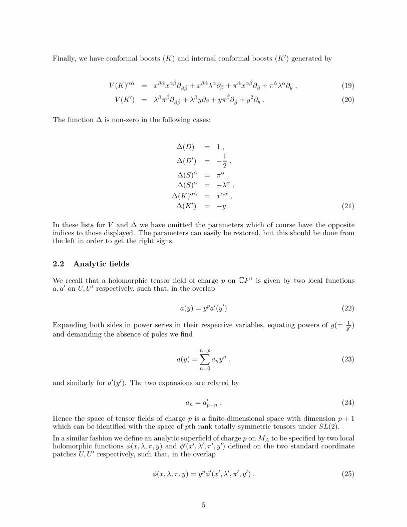
For completeness we reproduce here the explicit expressions for the vector fields correspondingto the different types of superconformal transformation. From (6) one can read off the vectorfields for each of the parameters. They divide into translational (B), linear (A,D) and quadratic(C) types. The translations are ordinary spacetime translations, half of the Q-supersymmetrytransformations and translations in the internal y space, CP 1. The corresponding vector fieldsare

VAA′ =∂

∂XAA′. (9)

The linearly realised symmetries are Lorentz transformations (SL(2)×SL(2)) in complex space-time) and dilations, internal dilations, R-symmetry transformations, the other half of the Q-supersymmetries and half of the S-supersymmetries. The Lorentz transformations are handledin the usual way so that we do not need to write them down. The vector fields generatingdilations (D), internal dilations (D′) and R-symmetry transformations are

V (D) = xαα∂αα +1

2(λα

′

∂α + πα∂α) , (10)

V (D′) = y∂y +1

2(λα∂α + πα∂α) , (11)

V (R) = λα∂α − πα∂α . (12)

The vector fields generating linearly realised Q-supersymmetry are

V (Q)α = πα∂αα + y∂α , (13)

V (Q)α = λα∂αα − y∂α , (14)

while those generating linearly realised S-supersymmetry are

V (S)α = xαα∂α + λα∂y , (15)

V (S)α = xαα∂α − πα∂y . (16)

The remaining supersymmetry transformations are the non-linearly realised S-supersymmetriesgenerated by

V (S)α = xβαπβ∂ββ + xβαy∂β − παπβ∂β − παy∂y , (17)

V (S)α = −λβxαβ∂ββ − λβλα∂β + yxαβ∂β + yλα∂y . (18)

4

Finally, we have conformal boosts (K) and internal conformal boosts (K ′) generated by

V (K)αα = xβαxαβ∂ββ + xβαλα∂β + παxαβ∂β + παλα∂y , (19)

V (K ′) = λβπβ∂ββ + λβy∂β + yπβ∂β + y2∂y . (20)

The function ∆ is non-zero in the following cases:

∆(D) = 1 ,

∆(D′) = −1

2,

∆(S)α = πα ,

∆(S)α = −λα ,∆(K)αα = xαα ,

∆(K ′) = −y . (21)

In these lists for V and ∆ we have omitted the parameters which of course have the oppositeindices to those displayed. The parameters can easily be restored, but this should be done fromthe left in order to get the right signs.

2.2 Analytic fields

We recall that a holomorphic tensor field of charge p on CP 1 is given by two local functionsa, a′ on U,U ′ respectively, such that, in the overlap

a(y) = ypa′(y′) (22)

Expanding both sides in power series in their respective variables, equating powers of y(= 1y′ )

and demanding the absence of poles we find

a(y) =

n=p∑

n=0

anyn . (23)

and similarly for a′(y′). The two expansions are related by

an = a′p−n . (24)

Hence the space of tensor fields of charge p is a finite-dimensional space with dimension p + 1which can be identified with the space of pth rank totally symmetric tensors under SL(2).

In a similar fashion we define an analytic superfield of charge p onMA to be specified by two localholomorphic functions φ(x, λ, π, y) and φ′(x′, λ′, π′, y′) defined on the two standard coordinatepatches U,U ′ respectively, such that, in the overlap

φ(x, λ, π, y) = ypφ′(x′, λ′, π′, y′) . (25)

5

If we now expand both sides in the odd variables and in y or y′, we obtain restrictions on thecomponent functions. For example, the zeroth order term in λπ is an x-dependent charge pholomorphic tensor on CP 1, the component of λ behaves like a tensor of charge p − 1 and soon. In addition, since the relation between x and x′ involves a shift, spacetime derivatives willappear in the constraints.

The basic superfield we shall consider is the hypermultiplet. In this language this multiplet isrepresented by an analytic superfield φ of charge 1. Using the above method one can easily seenthat it has only a short expansion:

φ(x, λ, π, y) = ϕ(x, y) + λαψα(x) + παχα(x) + λαπαϕαα(x) (26)

Furthermore

ϕ(x, y) = ϕo(x) + yϕ1(x) (27)

and similarly for ϕ′(x′, y′), with

ϕo = ϕ′1; ϕ1 = ϕ′

o . (28)

We also find

ϕαα = −∂ααϕ1; ϕ′αα = ∂ααϕo . (29)

In addition, the fields ϕo, ϕ1, ψ, χ must all satisfy their equations of motion

�ϕo = �ϕ1 = 0 ,

∂ααψα = 0 ,

∂ααχα = 0 . (30)

This is the usual hypermultiplet with two complex scalar fields and two complex Weyl fermions,all of which are physical and on-shell. In the interacting theory, the on-shell hypermultiplet willbe covariantly analytic, but gauge-invariant products of hypermultiplets will be analytic tensorfields of the type we have just described with charges 2, 3, . . .. For example, a field of chargetwo contains an independent vector field vαα, which is conserved, but there are no equations ofmotion. In other words a charge two field is a linear multiplet.

2.3 Correlation functions and Ward identities

In this section we consider the superconformal Ward identities for four-point correlation func-tions for analytic operators with charges p1, p2, p3, p4. We shall denote such correlators by< p1p2p3p4 >. Note, however, that the operators are not assumed to be the same even if theyhave the same charges, in particular, we shall not impose any symmetry requirements on suchcorrelators.

If we assume that analyticity holds in the quantum theory, the superconformal Ward identityfor such a correlator reads

4∑

i=1

(Vi + pi∆i) < p1p2p3p4 >= 0 (31)

6

The assumption of analyticity is tantamount to using the field equations of the underlyinghypermultiplet at operator level. This should be reasonable provided that we keep the pointsseparated. In the case of charge two operators, which is the main focus of this paper, the H-analyticity condition implies, as we noted above, that the superfield describes a linear multipletwith a conserved spacetime current. Analyticity can be examined directly in perturbation theoryusing the harmonic superspace formalism and has been verified in all the examples that havebeen looked at so far.

We shall consider correlators of the above type which have non-vanishing leading terms. Further,we will specialise to correlators with four equal charges p. In this case we can write

< pppp >= (g12)p(g34)

pF (32)

where gij is the free two-point function for charge one operators at points i and j,

gij = sdetX−1ij =

yijx2ij

(33)

and F is an arbitrary function of invariants. Here Xij = Xi − Xj denotes the coordinatedifference matrix for points i and j and

yij = yij − πijx−1ij λij (34)

with the index convention that x−1 has a pair of subscript indices αα.

It is straightforward to check that gij satisfies the equation

(Vi + Vj +∆i +∆j)gij = 0 (35)

so that the Ward identity for < pppp > will indeed be satisfied for any invariant F .

It is not difficult to see that there must be more N = 2 analytic superconformal invariants thanthere are spacetime conformal invariants for four points. If we expand F in the odd variables λand π the leading term must be invariant under spacetime conformal transformations and alsounder conformal (SL(2)) transformations of CP 1. At four points there are two independentspacetime (x) cross-ratios and one independent internal (y) cross-ratio, so that there shouldbe at least three independent analytic superconformal invariants at four points. In fact, thereare no more. Any additional independent invariant would have to be nilpotent, but one caneasily show that there are no such invariants at four points. The reason is essentially dueto counting; there are 4 × 4 = 16 odd coordinates which is precisely equal to the number ofsupersymmetries in SL(4|2). On a putative nilpotent invariant these supersymmetries behaveessentially like translational symmetr! ies so that any possible leading term must vanish. Inmore detail, suppose that F is a nilpotent four-point invariant. It can be written Fo + ... whereFo is the term with the lowest power of λπ. By examining the supersymmetry transformationsdirectly one can see that the first term in the variation of F involves only Fo. Furthermore,again by looking at each transformation in turn, one finds that setting this first term in thevariation equal to zero (because F is an invariant) leaves no possible solutions for separatedpoints. Consequently one concludes that there can be no nilpotent invariants. This argumentis presented in detail in [20].

It was shown in [6] that non-nilpotent analytic superspace superconformal invariants can beexpressed in terms of superdeterminants and supertraces of the coordinate differences Xij . Forthe case in hand a possible choice of three independent invariants is given as follows: we taketwo super cross-ratios

7

S =sdetX14sdetX23

sdetX12sdetX34, T =

sdetX13sdetX24

sdetX12sdetX34(36)

and one supertrace invariant

U = str(X−112 X23X

−134 X41) . (37)

The invariants S and T may be expressed in terms of the spacetime cross-ratios

s =x214x

223

x212x234

, t =x213x

224

x212x234

(38)

and the internal cross-ratio

v =y14y23y12y34

(39)

in the form

S =s

v, T =

t

w. (40)

Here w = y13y24y12y34

= 1+ v, and the hats on v and w are defined by hatting each of the y variables

in their definitions,

v =y14y23y12y34

, w =y13y24y12y34

. (41)

We may write

w = 1 + v +∆w (42)

and express the third invariant U in the form

U = 1− t+ s+ v +∆U . (43)

Both ∆W and ∆U are nilpotent quantities. The explicit expressions are as follows:

∆U =1

y12y34

(

− y12Π2x132Λ2 + y34Π1x

423Λ1

+y23(

Π1x421Λ1 −Π2x

134Λ2 −Π1x

421Λ2 +Π2x

134Λ1

)

+(Π1x23Λ2)(Π2x23Λ1))

(44)

and

8

∆w =1

y12y34

(

− y12Π2x432Λ2 + y34Π1x

123Λ1

+y23(

Π1[x123 − x124]Λ1 +Π2[x

431 − x432]Λ2 +Π1x

124Λ2 −Π2x

431Λ1

)

−(Π1x321Λ1)(Π2x

234Λ2)

)

(45)

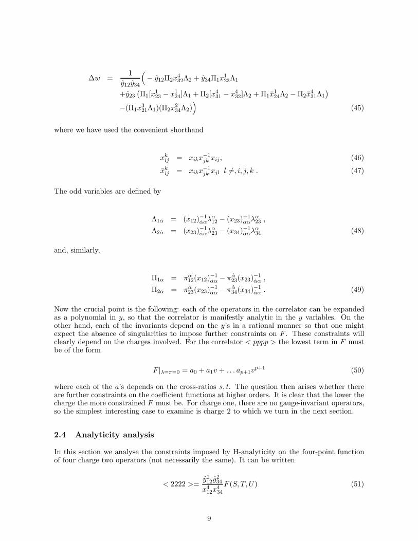
where we have used the convenient shorthand

xkij = xikx−1jk xij, (46)

xkij = xikx−1jk xjl l 6=, i, j, k . (47)

The odd variables are defined by

Λ1α = (x12)−1ααλ

α12 − (x23)

−1ααλ

α23 ,

Λ2α = (x23)−1ααλ

α23 − (x34)

−1ααλ

α34 (48)

and, similarly,

Π1α = πα12(x12)−1αα − πα23(x23)

−1αα ,

Π2α = πα23(x23)−1αα − πα34(x34)

−1αα . (49)

Now the crucial point is the following: each of the operators in the correlator can be expandedas a polynomial in y, so that the correlator is manifestly analytic in the y variables. On theother hand, each of the invariants depend on the y’s in a rational manner so that one mightexpect the absence of singularities to impose further constraints on F . These constraints willclearly depend on the charges involved. For the correlator < pppp > the lowest term in F mustbe of the form

F |λ=π=0 = a0 + a1v + . . . ap+1vp+1 (50)

where each of the a’s depends on the cross-ratios s, t. The question then arises whether thereare further constraints on the coefficient functions at higher orders. It is clear that the lower thecharge the more constrained F must be. For charge one, there are no gauge-invariant operators,so the simplest interesting case to examine is charge 2 to which we turn in the next section.

2.4 Analyticity analysis

In this section we analyse the constraints imposed by H-analyticity on the four-point functionof four charge two operators (not necessarily the same). It can be written

< 2222 >=y212y

234

x412x434

F (S, T, U) (51)

9

The invariants S, T, U are convenient from some points of view - it is easy to see that they areinvariants, and they have concise explicit forms. Requiring H-analyticity implies that F shouldhave no singularities in (y13, y14, y23, y24) and that it can have poles up to order two in (y12, y34)(if we had charge p operators this would become order p). Since (y12y34) occurs as a denominatorin S−1, T−1 and U the regularity of the correlator will lead to constraints for F .

Note that regularity in the hatted variables is equivalent to regularity in the unhatted ones: ifwe demand that the whole correlator be a polynomial in the hatted y’s and write, for example,y12 = y12 + δ12, then a Taylor expansion will produce a polynomial of the same degree in theunhatted y’s, because the δ’s are non-singular and y-independent.

Clearly, H-analyticity should hold at each order in the odd variables separately. We shall carryout the expansion in two steps: we first expand in the nilpotent quantities ∆U,∆w and thenexpress the latter in terms of products of spinors. We will here refer to the order in ∆U, ,∆w as“level” in order to distinguish the first from the second step. The main technical problem onefaces in this approach is to compute which of the various products of the form (∆u)p(∆w)q areindependent for each fixed value of p+ q, i.e. at a given “level”.

From the point of view of expanding in odd variables it is helpful to think about an equivalentset of invariants, S′, T ′, V , which are defined to have leading terms s, t and v respectively. Theseinvariants are expressed in terms of S, T, U by

S′ = SV, T ′ = T (1 + V ), V =T + U − 1

1 + S − T(52)

Since we have

S′ = s+ . . . (53)

T ′ = t+ . . . (54)

V = v + . . . (55)

it follows from (51) that we may write F in the form

F = a1(S′, T ′) + a2(S

′, T ′)V + a3(S′, T ′)V 2 . (56)

This expression clearly meets the lowest level requirements of analyticity for charge 2 and showsthat the dependence on the third invariant V is thereby fixed. The objective now is to Taylorexpand F about S′ = s, T ′ = t and V = v. However, since the original set of invariants is easierto evaluate explicitly, we shall convert the Taylor expansion back into these variables as we go.In this way we arrive at a power series in the nilpotent quantities ∆U and ∆w. We will thenexpress both of these and the coefficients that accompany them in terms of the set of coordinates(x12, x23, x34, y12, y23, y34,Λ1,Λ2,Π1,Π2). These variables are convenient in the sense that theyare invariant under translational Q-supersymmetry and linear S-supersymmetry, and in additionthey involve no y-singularities. Furthermore, as noted above, the difference between y and y isnon-singular so it is permissible to study analyticity in the latter rather than the former.

The Taylor expansion of F is then

F (S, T, U) = Fo +∆U(∂UF ) + ∆w(− tw2 ∂TF )

12∆U

2(∂2UF ) + ∆U∆w(− tw2∂U∂TF ) +

12∆w

2( t2

w4∂2TF + 2 t

w3 ∂TF ) + ... (57)

where Fo is F (S′, T ′, V ) evaluated at (s, t, v). Clearly

10

Fo = a1(s, t) + a2(s, t)v + a3(s, t)v2 . (58)

In the new variables the partial derivatives, evaluated at (S′, T ′, v), are

∂U =1

RD ,

∂T =(1 + v)

R(D +R∂t) (59)

with

R = s+ v − v t

1 + v,

D = s ∂s + v ∂v +v t

1 + v∂t . (60)

Here v has been replaced by v because we wish to use the Taylor expansion about the point(s, t, v). We will almost always multiply R and D by w = 1+ v in order to avoid the singularityin their denominators. Note that DR = R.

We shall refer to the expressions in round brackets multiplying a certain power ∆Up∆wq in(57) as “component functions”. The expansion ends at fourth order, because ∆U,∆w are R-symmetric and are therefore power series in (ΠΛ). Since the spinors are two-component objectsand since there are two Π’s and two Λ’s it follows that the highest possible power is (ΠΛ)4.

Let us investigate the linear level in the Taylor expansion. We ask whether singularities in ∆Uand ∆W can conspire to cancel or whether the latter are independent objects. The componentfunctions depend on s, t, v, which yields a linear dependence problem with coefficients in thering of functions of s, t, v.

The functional form of these coefficients can be made much more explicit. Given the form ofF (58), by commuting all R’s to the left and all ∂t’s to the right we can show that the generalcomponent functions at k-th level have the form

1

(w(wR))k

2+2k∑

n=0

cn(s, t) vn . (61)

The extra factors w in the denominator are introduced by the coefficients of the ∂T derivativesand obviously factor out in the pure (∂U )

k component functions. A direct computer calculationshows them to cancel in the other components, too. Without enhanced factorisation abilities thispoint is hard to show and therefore we keep the w’s in the scheme. Incidentally, by introducingτ = 1/T the component functions can be more easily computed: They are simply

1

tn∂nτ ∂

mU F . (62)

We now examine the first order independence problem in detail. We work to lowest order, sothe hat on v is left out in the following and R0 denotes the body of R. For charge two operatorsanalyticity requires that there be functions of (s, t) for ∆U and ∆w such that

11

∆U1

w(wR0)(

4∑

n=0

c0n(s, t)vn) + ∆w

1

w(wR0)(

4∑

n=0

c1n(s, t)vn) = O(

1

(y12 y34)2) (63)

with w = 1 + v.

Spinors occur in ∆U,∆w in combinations of the form (Πxx−1 xΛ). Minkowski space is four-dimensional; a basis consists of four independent elements. In order to express the variousx-triples in a given basis, we use

xix†j + xjx

†i = 2(xi.xj) δ (64)

to commute x12 left of x23 left of x34. ((xi.xj) means the dot product of the associatedfour-vectors.) In this way the spinors are seen to be contracted on elements of the basis

{x12, x23, x34, x12x†23x34}.There are two Πi and two Λi so that we get a total of sixteen independent structures at firstorder in (ΠΛ). A dependence relation between ∆U and ∆w is a linear combination with scalarcoefficients which is of a certain order in y-singularities in all sixteen components separately.We restrict the analysis to the (Π1Λ2) part of the odd expansion:

∆U |Π1Λ2= − y23

y12 y34Π1(x

234 x12 + x214 x23 + x212 x34 + x12x

†23x34)Λ2 , (65)

∆w|Π1Λ2= − y23

y12 y34Π1(x

234 x12 + x212 x34 + x12x

†23x34)Λ2 (66)

which we write in short as

∆U |Π1Λ2= − y23

y12 y34Π1XUΛ2 , (67)

∆w|Π1Λ2= − y23

y12 y34Π1XwΛ2 . (68)

On Minkowski space we change basis to {XU ,Xw, x12, x34} upon which the equation (63) breaksinto two separate parts. We can omit the spinors and the x-vectors from the discussion as theyhave to be equal on both sides of the equations. This leads to the scalar equation

− y23y12 y34

(4

∑

i=0

cn(s, t)vn = (1 + v)(s+ v(1 + s− t) + v2)O(

1

(y12 y34)2) (69)

for both the ∆U and ∆W parts.

Instead of the variables {y12, y23, y34} we may choose the set {v, Yp = y23/(y12y34), y23}. TheJacobian of the transform is

J =y223

(y12 y34)3(y12 − y34) (70)

and is regular at a generic point. Given this choice, the L.H.S. of (69) is independent of y23and factors out a single power of Yp. We can conclude that the same is true for the R.H.S. andhence the as yet unspecified term is a function of s, t, v of maximum order 1/(y12 y34). It mustbe a polynomial of degree 1 in v.

12

It follows that the ansatz polynomial on the L.H.S. factors in the same way and w(wR0) cancelsfrom the equation. The only solution of the regularity problem at first order is therefore thetrivial one:

∆U (1

∑

n=0

gn(s, t)vn) + ∆w (

1∑

n=0

hn(s, t)vn) = O(

1

(y12 y34)2) (71)

This is a general solution because ∆U and ∆w are not more singular than 1/(y12 y34) in anyof the components w.r.t. the sixteen independent structures at first order. By inspection, thehigher order terms arising from the second order in ∆U,∆W and from the soul of v will also beregular.

Let us state the result again: The explicit forms for the level one component functions in theTaylor expansion (57) must have the dependence on v indicated by the above equation. Hence

DFo

R= g1 + vg2 (72)

and

(D +R∂t)Fo

wR= h1 + vh2 . (73)

We ought to stress that the proof makes use of certain regularity assumptions. Throughout thecalculation we have assumed the x-scalars and in particular s and t to be regular. Hence noneof the four points can be light-like separated in Minkowski space. This can possibly be relaxed.A necessary assumption is certainly that the vector basis is non-degenerate, so in particular thepoints do not coincide. For the y-coordinates we must also demand that the points are distinct.For the Jacobian (70) to be non-vanishing we additionally need y12 6= y34.

If y34 = αy12 we can change from {y12, y23} to {y23/(α y212), v}. In this case (69) still has thesame consequences: The prefactor must occur on both sides and drops out. The unknown parton the R.H.S. is a function of s, t, v as before. The Jacobian of the transformation is

J =y23α2 y512

((1 + α) y12 + 2 y23) (74)

and hence is regular if the points do not coincide and y12 is not proportional to y23, so if thereis more than one difference variable. The argument holds in fact as long as two of the yij areindependent. Otherwise v is a constant and there is nothing to discuss.

The generalisation of the independence problem (63) to the higher levels like ∆U2, ∆U∆w, ...is obvious. We have investigated this in the same manner to lowest order and we find that thespinor combinations are not independent. Additionally, the simple argument does not apply,which allowed us to ignore higher orders stemming from the lower level terms in the Taylorexpansion (57). These terms define a non-trivial right hand side in the equivalent of (63) inthe levels above. Due to linearity it suffices to find one special solution to this inhomogeneousproblem which is to be added to the general solution of the homogeneous one.

To analyse equation (72) we begin by multiplying it by (1 + v)R which gives a polynomialequation in v. This allows us to express the unknown functions g1, g2 in terms of a1, a2, a3,

g1 = a1s , g2 = a1s + a1t − a2t + a3t (75)

13

where the literal subscripts denote partial derivatives. This leaves two first-order partial differ-ential equations for a1, a2, a3,

(t− s− 1)a1s + (t− s)a1t + s(a2s + a2t) + a2 − sa3t = 0 ,

−a1s − a1t + a2t + sa3s + (t− 1)a3t + 2a3 = 0 .

(76)

If we make the change of variables

a1 = α+ γ + sa3 ,

a2 = γ + (s− t+ 1)a3 (77)

with a3 unchanged, we find that a3 drops out of the above equations altogether - it is completelyundetermined. The equations are satisfied if

αs + αt + γs = 0 ,

tγt + γ + (1− s)αt − sαs = 0 . (78)

This pair of first-order coupled differential equations can be equivalently rewritten as a set ofsecond-order independent ones:

sαss + tαtt + (s + t− 1)αst + 2(αs + αt) = 0 ,

sγss + tγtt + (s+ t− 1)γst + 2(γs + γt) = 0 . (79)

Note that in the correlator there is still one arbitrary coefficient function (a3(s, t) for this choiceof variables) in addition to the solutions to these equations.

When carrying out this type of analysis for the higher level regularity problems, we find that thedependence relations between ∆Uk etc. introduce so many unknowns into the equations thatno new constraints are found. We have done these calculations for operator weight one throughthree with the result that the only constraints arise from the first level.

3 SU(2)-covariant approach

In this section we explain how the four-point function results obtained in the first part ofthis paper can be found in an independent way in a harmonic superspace formulation whichmaintains the explicit SU(2) covariance. The technique is quite different, the main point beingthat here we shall keep Q supersymmetry (including its SU(2) automorphism) manifest at eachstep. However, S supersymmetry, as well as harmonic analyticity will have to be checked levelby level in the θ expansion of the four-point function. The advantage of this approach is thepossibility to reformulate the H-analyticity condition in an equivalent way which will allow usto essentially eliminate the dependence on the G-analytic Grassmann variables. After this theconstraints at levels 1 and 2 become sufficiently easy to work out. Moreover, it becomes obviousthat there are no constraints beyond level 2.

14

3.1 SU(2) harmonics and Grassmann analyticity

As discussed in the previous section N = 2 harmonic superspace is the product of superMinkowski space (coordinates (xµ ∼ xαα, θαi , θ

αi)) and the two-sphere. However, in this sec-tion, rather than using explicit coordinates (y, y) for the sphere, we shall use an alternativeapproach first proposed in [17] in which the sphere is described by harmonic variables u±i de-fined as the two columns of an SU(2) matrix; the index i transforms under the (left) SU(2) and± under an independent (right) U(1) group. The components of u have the defining properties:

(

u+1 u−1u+2 u−2

)

∈ SU(2) ⇒ u−i = (u+i)∗ , u+iu−i = 1 (80)

where the SU(2) indices are raised and lowered in the following way, f i = ǫijfj , fi = ǫijfj with

ǫij defined by ǫ12 = −ǫ12 = 1.

The harmonic functions f q(u±i ) are defined as singlets of the left SU(2) but they are homogeneousof degree q under the right U(1), i.e. carry a charge q. Effectively, such functions live on the cosetSU(2)/U(1) ∼ S2 and are assumed to have a harmonic expansion on the sphere. A powerfulfeature of the coordinateless parametrisation of S2 in terms of harmonics u±i is the possibilityto write down such expansions in a manifestly SU(2) covariant way, e.g., for q ≥ 0:

f q(u) =

∞∑

n=0

f (i1...in+qj1...jn)u+i1 . . . u+in+q

u−j1 . . . u−jn. (81)

The coefficients in this expansion are totally symmetric multispinors, i.e. irreps of SU(2) ofisospins q/2 + n , n = 0, 1, . . .. Thus, using harmonic variables allows one to deal with U(1)covariant objects without loosing the SU(2) symmetry.

With the aid of u we can define Grassmann analyticity in an SU(2)-covariant way. We split theGrassmann variables θαi , θ

αi into two U(1) projections,

θ±α = u±i θiα, θ±α = u±i θ

iα , (82)

still maintaining the SU(2) invariance. We then define a G-analytic function φ on harmonicsuperspace to be one which satisfies

D+α φ = D+

α φ = 0 (83)

where the U(1) projections of the supercovariant derivatives are defined in a similar way. Theseconstraints are solved by

φ = φ(xA, θ+α, θ=α) (84)

where

xααA = xαα − 4iθ(i αθj) αu+i u−j (85)

with xαα = xµσααµ . Clearly G-analyticity is a Q-supersymmetric notion because it involves thesupercovariant derivatives.

As explained in the previous section, complexified analytic superspace can be defined as a cosetspace of the complex superconformal group. Although this is not possible in real spacetime

15

we can nevertheless define a representation of the Lie superalgebra of SU(2, 2|2) on G-analyticfields. For all practical purposes this amounts to taking infinitesimal SU(2) transformations(parameters λjk) to have the form u±i :

δu+i = (λjku+j u+k ) u

−i , δu−i = 0 . (86)

More generally, it is sufficient to treat the transformations of the harmonic variables u±i with

generators K,D,R, S, I as active ones. For instance, a harmonic function f (p)(u) of weight pwill transform as follows:

δf (p)(u) = f ′(p)(u)− f (p)(u)

= −(λiju+i u+j )u

−k

∂

∂u+kf (p)(u) + p(λiju−i u

+j )f

(p)(u) , (87)

so that the non-unitary transformation appears in the form of a derivative of a function ofunitary harmonics.

Henceforth we shall be dealing exclusively with G-analytic fields so that we can replace xA byx without loss of clarity. The actions of the supersymmetry transformations on the coordinatesare given by

δQxαα = −4iu−i (ǫ

iαθ+α + θ+αǫiα)

δQθ+α,α = u+i ǫ

iα,α

δQu±i = 0 (88)

and [24]

δSxαα = 4i(xαβ θ+αηi

β− xαβθ+αηiβ)u

−i

δSθ+α = −2i(θ+)2ηαiu−i + xαβ ηi

βu+i

δSθ−α = 4iηiβθ

−β(θ−αu+i − θ+αu−i ) + ηiβ(xαβ + 4iθ−αθ+β)u−i

δSu+i = [4i(θ+αηiα + ηiαθ

+α)u+i ]u−i

δSu−i = 0 (89)

(δS θ± are obtained by conjugation). From this one can compute the action of the rest of the

superconformal algebra by commuting Q and S supersymmetry transformations.

3.2 The hypermultiplet

In this subsection we give the harmonic formulation of the hypermultiplet describing an SU(2)doublet of scalars f i(x) and a pair of Weyl (complex) spinors ψα(x), ξ

α(x) on shell. Off shellit can only exist with an infinite set of auxiliary fields [26]. Such a set is naturally provided bythe G-analytic superfield of U(1) charge +1:

q+(x, θ+, θ+, u) = F+(x, u) + θ+αΨα(x, u) + θ+α Ξα(x, u) + ...+ (θ+)2(θ+)2P−3(x, u) . (90)

16

The components of this θ+ expansion are harmonic functions with infinite expansions on S2 (see(81)):

F+(x, u) = f i(x)u+i + f (ijk)(x)u+i u+j u

−k + . . .

Ψα(x, u) = ψα(x) + ψ(ij)α (x))u+i u

−j + . . .

. . .

P−3(x, u) = p(ijk)(x)u−i u−j u

−k + . . . (91)

The coefficients in these expansions are ordinary fields belonging to different SU(2) representa-tions. All of them, with the exception of the physical fields f i(x), ψα(x), ξ

α(x) are auxiliary, sothey should vanish on shell. We need a way to write down a supersymmetric on-shell constrainton the G-analytic superfield q+(x, θ+, θ+, u).

The key to this on-shell constraint is provided by the notion of harmonic (H-)analyticity. Theharmonic coset SU(2)/U(1) has two real (or one complex) dimensions, to which correspond thefollowing harmonic derivatives:

∂++ = u+i∂

∂u−i⇒ ∂++u+i = 0 , ∂++u−i = u+i ,

∂−− = u−i∂

∂u+i⇒ ∂−−u+i = u−i , ∂−−u−i = 0 . (92)

These are Cartan’s covariant derivatives on the coset. In our context this simply means thatthey preserve the defining condition u+iu−i = 1. To them one may add the charge-countingoperator

∂0 = u+i∂

∂u+i− u−i

∂

∂u−i⇒ ∂0u±i = ±u±i . (93)

By definition all harmonic functions are eigenfunctions of ∂0, ∂0f q(u) = qf q(u).

An important point is that the three covariant derivatives above form an SU(2) algebra:

[

∂++, ∂−−]

= ∂0 ,[

∂0, ∂±±]

= ±2∂±± . (94)

They can be regarded as the generators of right SU(2)R rotations acting on the indices ± of theharmonics u±i . Thus, ∂++ is the raising and ∂−− the lowering operator of SU(2)R (see (92)).This observation suggests the way to define short harmonic functions as highest weights of irrepsof SU(2)R. Thus, depending on the value of the U(1) charge, the condition

∂++f q(u) = 0 ⇒{

f q(u) = 0, q < 0

f q(u) = u+i1 . . . u+iqf (i1...iq), q ≥ 0

(95)

has either a trivial solution or defines an irrep of isospin q/2. This property is a direct conse-quence of the general form (81) of the harmonic expansion on S2 and of the action of ∂++ onthe harmonics (92).

An alternative interpretation of the condition (95) is that of harmonic (H-)analyticity. Let usintroduce stereographic coordinates on the sphere (see [27] for more detail):

17

(

u+1 u−1u+2 u−2

)

=1√

1 + yy

(

1 −yy 1

)

. (96)

Our harmonic functions f q(u) are by definition eigenfunctions of the charge “operator” ∂0:

∂0f q(y, y) = qf q(y, y) . (97)

In this parametrisation the covariant derivative ∂++ becomes

∂++ = −(1 + yy)∂

∂y− y

2∂0 . (98)

In these terms eq. (95) takes the form of a (covariant) harmonic analyticity condition:

∂f q

∂y+

qy

2(1 + yy)f q = 0 . (99)

It admits the general solution f q(y, y) = (1+yy)−q

2 f0(y) where f0(y) is an arbitrary holomorphicfunction. Remembering that we are looking for solutions globally defined on the sphere it is nothard to show that for q < 0 the only solution is f0 = 0 and for q ≥ 0 f0(y) must be a polynomialof degree q whose SU(2) covariant form is given in (95).

It should be stressed that the above H-analytic harmonic functions are regular, i.e. well-definedon the whole of S2. In practice one has also to deal with singular harmonic functions. A typicalexample we shall encounter in what follows is the harmonic distribution

1

(12)(100)

where

(12) ≡ u+i1 u+2i =

y2 − y1√

(1 + y1y1)(1 + y2y2). (101)

At first sight, it is a function of u+ only, therefore one would expect ∂++1 (12)−1 = 0. However,

this distribution is singular at the point u1 = u2, so it should be differentiated with care:

∂++1

1

(12)= (1 + y1y1)

3/2(1 + y2y2)1/2 ∂

∂y1

1

y1 − y2

= (1 + y1y1)2iπδ(y1 − y2)

= (12−)δ(u1, u2) , (102)

where we have used the well-known relation

∂

∂y

1

y= iπδ(y) . (103)

Note that the factor (12−) ≡ u+i1 u−2i is needed for keeping the balance of charges on both sides

of eq. (102) in the S(2) covariant notation.

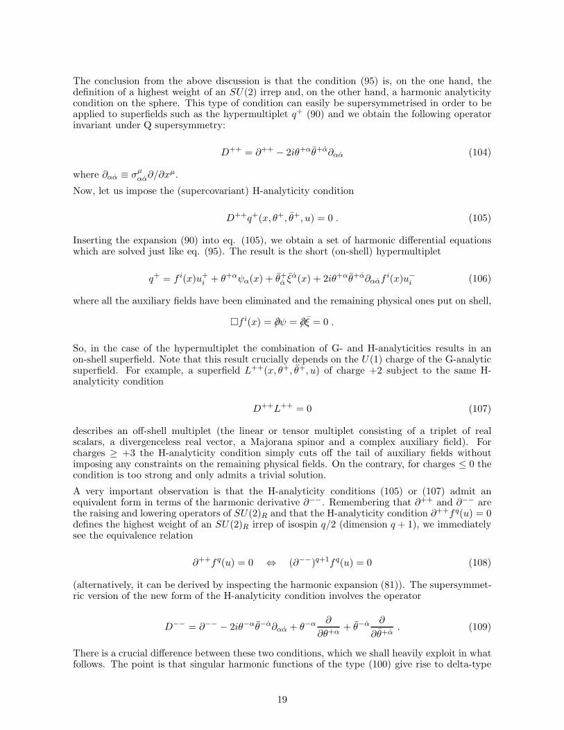
18

The conclusion from the above discussion is that the condition (95) is, on the one hand, thedefinition of a highest weight of an SU(2) irrep and, on the other hand, a harmonic analyticitycondition on the sphere. This type of condition can easily be supersymmetrised in order to beapplied to superfields such as the hypermultiplet q+ (90) and we obtain the following operatorinvariant under Q supersymmetry:

D++ = ∂++ − 2iθ+αθ+α∂αα (104)

where ∂αα ≡ σµαα∂/∂xµ.

Now, let us impose the (supercovariant) H-analyticity condition

D++q+(x, θ+, θ+, u) = 0 . (105)

Inserting the expansion (90) into eq. (105), we obtain a set of harmonic differential equationswhich are solved just like eq. (95). The result is the short (on-shell) hypermultiplet

q+ = f i(x)u+i + θ+αψα(x) + θ+α ξα(x) + 2iθ+αθ+α∂ααf

i(x)u−i (106)

where all the auxiliary fields have been eliminated and the remaining physical ones put on shell,

�f i(x) = ∂/ψ = ∂/ξ = 0 .

So, in the case of the hypermultiplet the combination of G- and H-analyticities results in anon-shell superfield. Note that this result crucially depends on the U(1) charge of the G-analyticsuperfield. For example, a superfield L++(x, θ+, θ+, u) of charge +2 subject to the same H-analyticity condition

D++L++ = 0 (107)

describes an off-shell multiplet (the linear or tensor multiplet consisting of a triplet of realscalars, a divergenceless real vector, a Majorana spinor and a complex auxiliary field). Forcharges ≥ +3 the H-analyticity condition simply cuts off the tail of auxiliary fields withoutimposing any constraints on the remaining physical fields. On the contrary, for charges ≤ 0 thecondition is too strong and only admits a trivial solution.

A very important observation is that the H-analyticity conditions (105) or (107) admit anequivalent form in terms of the harmonic derivative ∂−−. Remembering that ∂++ and ∂−− arethe raising and lowering operators of SU(2)R and that the H-analyticity condition ∂++f q(u) = 0defines the highest weight of an SU(2)R irrep of isospin q/2 (dimension q + 1), we immediatelysee the equivalence relation

∂++f q(u) = 0 ⇔ (∂−−)q+1f q(u) = 0 (108)

(alternatively, it can be derived by inspecting the harmonic expansion (81)). The supersymmet-ric version of the new form of the H-analyticity condition involves the operator

D−− = ∂−− − 2iθ−αθ−α∂αα + θ−α ∂

∂θ+α+ θ−α ∂

∂θ+α. (109)

There is a crucial difference between these two conditions, which we shall heavily exploit in whatfollows. The point is that singular harmonic functions of the type (100) give rise to delta-type

19

singularities under ∂++ (see (102)), whereas they can be differentiated as ordinary functions by∂−−, e.g.

∂−− 1

(12)= −(1−2)

(12)2. (110)

The explanation is that in the former case we deal with a derivative of the type ∂/∂y y−1 = iπδ(y)and in the latter ∂/∂y y−1 = −y−2.

In the rest of this section we shall examine the non-trivial implications of H-analyticity combinedwith the requirement of superconformal covariance for correlation functions of charge +2. Forthat purpose we shall need the superconformal transformation properties of the superfields andoperators we have introduced. The transformation law of the harmonic derivatives D++ andD−− can be found using Cartan’s coset scheme [27] (or checked directly [24]):

δD++ = −Λ++D0 ,

δD−− = −(D−−Λ++)D−− (111)

where

D++Λ = Λ++ , D++Λ++ = 0 (112)

and

Λ = a+ kααxαα + λiju+i u

−j + 4i(θ+αηiα + ηiαθ

+α)u−i (113)

is the superconformal weight factor. For completeness, besides the S supersymmetry parameterη we have also included those of dilation a, conformal boosts kµ and SU(2)C λij . Then it is nothard to check that the H-analyticity condition

D++q+ = 0 ⇔ (D−−)2q+ = 0 (114)

is covariant if the hypermultiplet transforms with superconformal weight +1:

δq+ = −λ · ∂q+ + Λq+ (115)

(here −λ · ∂ denotes the coordinate transformations). Similarly, the linear multiplet subject tothe H-analyticity condition

D++L++ = 0 ⇔ (D−−)3L++ = 0 (116)

should have weight +2:

δL++ = −λ · ∂L++ + 2ΛL++ . (117)

20

3.3 Two- and three-point functions

The simplest example of a two-point function is the hypermultiplet propagator

G(1,1)(1|2) = 〈q+(1)q+(2)〉 (118)

where the superscript (1, 1) indicates the U(1) charges at the two points and ˜ is a specialconjugation on S2 preserving G-analyticity [17]. It is defined as the Green’s function of the fieldequation (105):

D++1 G(1,1)(x1, θ

+1 , u1|x2, θ+2 , u2) = δ4(x1 − x2)(θ

+1 − (u+1 u

−2 )θ

+2 )

4(u−1 u+2 )δ(u1, u2) . (119)

Naturally, like the hypermultiplet superfield q+ itself, the Green’s function should be G-analytic.The right-hand side of eq. (119) is the complete delta-function of the G-analytic superspace (asin eq. (102), the factors (u+1 u

−2 ) and (u+1 u

−2 ) maintain the balance of U(1) charges). Throughout

this paper we assume that all the correlation functions are considered away from the coincidentpoints where they usually have singularities. In this case the right-hand side of eq. (119) justvanishes:

D++1 G(1,1)(1|2) = 0 for points 1 6= 2. (120)

The same is of course true if we replace D++1 by D++

2 . In other words, this two-point functionis H-analytic away from the singular point.

Another basic property of the hypermultiplet propagator is superconformal covariance. Accord-ing to the transformation law (115) of the hypermultiplet itself, the propagator transforms asfollows:

δG(1,1)(1|2) = −λ · ∂G(1,1)(1|2) + (Λ(1) + Λ(2))G(1,1)(1|2) . (121)

The combination of H-analyticity and the conformal properties of the propagator allow us tofind the explicit expression for G(1,1). We start by examining the leading component of thissuperfield

g(1,1)(x212, u1, u2) = G(1,1)(θ+1 = θ+2 = 0) . (122)

Here we have taken into account translation and Lorentz invariance which tell us that thefunction must depend on the space-time invariant x212 ≡ (x1 − x2)

2. In the absence of θ+ the

harmonic derivative D++ ≡ ∂++, so the H-analyticity condition (120) simply tells us that g(1,1)

must be linear in u+1 (recall (95)). At the same time it is an SU(2) invariant, so the index iof u+1i must be contracted with the other harmonic variable u±2 . Given the charges +1 at both

points, we conclude that the only such invariant combination of harmonics is (12) ≡ u+ii u+2i .

So, g(1,1) is reduced to

g(1,1) = (12)g(x212) . (123)

The remaining function g(x212) can be most easily determined by making use of the dilation partof the conformal group. The first component of the superfield q+ is the physical scalar f i(x)which has conformal weight 1, and so does the leading term in the hypermultiplet propagator.

21

The harmonic factor in (123) is weightless, so we conclude that g = C/x212. The constant C canbe fixed by comparing with the standard scalar propagator and the result is

g(1,1) =1

4iπ2(12)

x212. (124)

Now, the less trivial part of the determination of the propagator G(1,1) is completing it to a fullsuperfield, i.e. restoring the dependence on θ+1,2. Here we shall use a trick which will prove veryuseful in the study of the four-point correlator in the next subsection. The two-point functionis supposed invariant under Q supersymmetry (88), which acts as a shift of the Grassmannvariables:

(θ+α,α1,2 )′ = θ+α,α

1,2 + u+1,2iǫiα,α . (125)

It is then clear that by making a finite Q supersymmetry transformation with parameter

ǫiα,α =u+i2

(12)θ+α,α1 − u+i

1

(12)θ+α,α2 (126)

we can eliminate both θ+1 and θ+2 :

Q frame: (θ+α,α1 )′ = (θ+α,α

2 )′ = 0 . (127)

In this frame the two-point function becomes independent of the Grassmann variables. In otherwords, it coincides with its leading component (124), G(1,1)|Q ≡ g(1,1). Then we can go backto the original frame by performing the same finite Q supersymmetry transformations on theremaining coordinates.3 Such a transformation only affects the difference x12 and gives

xαα12 = xαα12 +4i

(12)[(1−2)θ+1 θ

+1 + (2−1)θ+2 θ

+2 + θ+1 θ

+2 + θ+2 θ

+1 ]

αα . (128)

By construction, this modified coordinate difference is invariant under Q supersymmetry, whichcan be easily verified using (88). So, to find out the θ+1,2 dependence of the hypermultipletpropagator, it is enough to replace x12 by x12:

G(1,1)(1|2) = 1

4iπ2(12)

x212. (129)

In deriving this two-point function we have only used the dilation part of the superconformalgroup. In fact, since the result is unique, it is guaranteed to have the right superconformalproperties (121) of the propagator (this can also be checked directly). Further, so far we haveonly solved the H-analyticity constraint (120) at the lowest (leading) order of the θ+ expansion.One might try to argue that since the left-hand side of eq. (120) is itself an invariant of Qsupersymmetry, it is sufficient to check H-analyticity in the Q frame (i.e., in the absence of θ+).However, this argument is not safe here. Indeed, in the expansion of the two-point functionthere are harmonic singularities of pole type (e.g., (12)−1), on which the operator ∂++ createsa delta-type singularity (recall (102)). In such a situation we will not be allowed to use the

3As a simpler example of this trick, consider translation invariance for a set of two space-time points x1, x2.By means of the finite translation P : x′

2 = x2 + a = 0 we can go to a P frame in which only x1 survives. Then,to restore manifest invariance, we make the same shift on x1: x

′

1 = x1 + a = x1 − x2 ≡ x12.

22

supersymmetry parameter (126) which itself contains harmonic poles. A safe way to extendH-analyticity to all orders in the θ+ expansion by means of the transformation (126) is to usethe alternative form of the H-analyticity constraint involving D−− (see (114)). We shall comeback to this important point in the next subsection.

Knowing the hypermultiplet propagator, we can easily predict the general form of correlators oftwo or three composite operators made out of hypermultiplets. Take, for instance, the two-pointfunction

G(2,2)(1|2) = 〈Tr(

q+(1))2

Tr(

q+(2))2〉 . (130)

Note that it has charges +2 at each point matching the number of elementary hypermultiplets ineach composite operator. One can imagine this correlator in the context of N = 4 super-Yang-Mills theory, where a hypermultiplet in the adjoint representation of the gauge group interactswith the N = 2 super-Yang-Mills gauge potential. Since the N = 4 theory is finite (conformallyinvariant), we can demand that the correlator (130) be superconformally covariant,

δG(2,2)(1|2) = −λ · ∂G(2,2)(1|2) + 2(Λ(1) + Λ(2))G(2,2)(1|2) . (131)

In addition to this, the correlator should be H-analytic. Indeed, let us differentiate it with theharmonic derivative D++.4 Since D++ is the operator of the free field equation (90) for thehypermultiplet, one can argue that such a differentiation will give rise to a Schwinger-Dysonequation for the correlator:

D++1 G(2,2)(1|2) = contact terms . (132)

Since the composite operators are bilinear in this case (charges +2), equation (132) can also beinterpreted as a Ward identity. Indeed, the bilinears q+q+, q+q+ and q+q+ are the currents ofan extra SU(2) symmetry of the N = 4 theory realised in terms of N = 2 superfields5. So, inthis case eq. (132) corresponds to the current conservation law. In the context of this paper wetreat contact terms as zeros, so eq. (132) takes the form of an H-analyticity condition:

D++1 G(2,2)(1|2) = 0 for points 1 6= 2 (133)

(and similarly at point 2). Since the product of two H-analytic functions is H-analytic as well,we immediately find an obvious solution to this constraint as the square of the hypermultipletpropagator,

G(2,2)(1|2) = C(12)2

x412(134)

where C is a constant. In fact, this is the general solution. The argument is as in the case ofthe propagator. One first examines the leading component G(2,2)(θ+1 = θ+2 = 0). The constraint(133) fixes the harmonic dependence since the combination (12)2 is the only SU(2) invariantof charges (2, 2) annihilated by ∂++. The dependence on x212 is determined by simple dilationcovariance. Finally, with two G-analytic Grassmann variables θ+1,2 we already know that the

complete θ+ dependence is fixed by Q supersymmetry alone, by just putting a hat on x212. Itshould be mentioned that the above considerations cannot predict the value of the constant in

4The traces in (130) make the composite operators gauge invariant, so we can use a flat D++ (no gaugeconnection).

5In fact, this symmetry is the visible part of the full SU(4) R symmetry of the N = 4 theory.

23

(134). In principle, it might receive quantum corrections at each level of perturbation theory,but it can be shown that this type of correlator is protected by a non-renormalisation theorem[5, 8].

Next we turn to three-point correlators. As an example, take the correlator of three currents,i.e. bilinears made out of hypermultiplets:

G(2,2,2)(1|2|3) = 〈Tr(

q+(1))2

Tr(

q+(2)q+(2))

Tr(

q+(3))2〉 (135)

and subject to the requirements of H-analyticity

D++1 G(2,2,2)(1|2|3) = 0 for points 1 6= 2 6= 3 (136)

and of superconformal covariance

δG(2,2,2)(1|2|3) = −λ · ∂G(2,2,2)(1|2|3) + 2(Λ(1) + Λ(2) + Λ(3))G(2,2,2)(1|2|3) . (137)

Just as for G(2,2)(1|2) above, it is obvious that the product of three propagators

G(2,2,2)(1|2|3) = C(12)

x212

(23)

x223

(31)

x231(138)

satisfies both requirements. To prove its uniqueness, we argue as follows. Firstly, at the lowestlevel in the θ+ expansion there is a single SU(2) invariant combination of the three harmonicswith the right charges and vanishing under D++

1 , namely (12)(23)(31). Secondly, the space-timedependence is now determined by the full conformal group (and not just dilations, as for twopoints). It is well-known that there exists no conformal invariant made out of three space-timevariables, therefore the product x−2

12 x−223 x

−231 is the only function with the required conformal

properties. Finally, we have to show that putting hats on the x’s gives the unique completionof the leading component to a full superfield. Before we did this by using the Q frame (127) inwhich the two Grassmann variables had been eliminated. Now we have three θ+’s, and the Qsupersymmetry parameter ǫi alone is not enough to shift away all of them. This time we haveto invoke S supersymmetry as well. Looking at the transformation law of θ+ in (89) we see thatS supersymmetry acts essentially as a shift (although non-linear), provided that the matrix xαα

is invertible. Then the combination of Q and S supersymmetry makes it possible to find a

Q&S frame: (θ+α,α1 )′ = (θ+α,α

2 )′ = (θ+α,α3 )′ = 0 (139)

in which there are no θ+’s left.6 So, if there existed another superfield completion of the leadingcomponent above, their difference would be a nilpotent (i.e., proportional to θ+) superconformalcovariant. But such an object would vanish in the Q&S frame, therefore it must vanish in anyframe. So, H-analyticity and superconformal covariance can predict the form of the three-pointcorrelator up to a constant factor. Once again, it turns out protected by a non-renormalisationtheorem [5, 8].

3.4 Four-point correlators

3.4.1 Preliminaries

The main subject of interest in this paper are four-point correlators of hypermultiplet bilinearsof the type, e.g.,

6In fact, the S supersymmetry parameter ηi is an SU(2) doublet, just as ǫi. Using both of them we can shiftaway up to four θ+, as we shall do in the four-point case.

24

G(2,2,2,2)(1|2|3|4) = 〈Tr(

q+(1))2

Tr(

q+(2))2

Tr(

q+(3))2

Tr(

q+(4))2〉 (140)

satisfying the requirements of H-analyticity

D++1 G(2,2,2,2)(1|2|3|4) = 0 for points 1 6= 2 6= 3 6= 4 (141)

and of superconformal covariance

δG(2,2,2,2)(1|2|3|4) = −λ · ∂G(2,2,2,2)(1|2|3|4) + 2(Λ(1) + Λ(2) + Λ(3) + Λ(4))G(2,2,2,2)(1|2|3|4) .(142)

Compared to the two- and three-point cases above, the structure of the four-point correlatoris considerably richer, for two main reasons which can be seen at the lowest level in the θ+

expansion. Firstly, now there exist three independent harmonic combinations satisfying (141):

(12)2(34)2 , (14)2(23)2 , (12)(23)(34)(41) . (143)

Any other combination can be reduced to these by means of the harmonic cyclic identity

(12)(34) + (13)(42) + (14)(23) = 0 (144)

following from the property of the ǫij contraction. Secondly, given four space-time points, onecan construct two independent conformal invariants,7 the cross-ratios

s =x214x

223

x212x234

, t =x213x

224

x212x234

. (145)

Consequently, the most general form of the leading component of the correlator (140) consistentwith H-analyticity and conformal covariance is

(12)2(34)2

x412x434

a(s, t) +(14)2(23)2

x414x423

b(s, t) +(12)(23)(34)(41)

x212x223x

234x

241

c(s, t) . (146)

Here we see the three independent harmonic structures (143) completed to product of propa-gators. Such products already have the required conformal properties of the correlator, so theonly freedom left are the three arbitrary coefficient functions a, b, c of the invariant cross-ratios.Our aim will be to find constraints on these functions following from the full implementation ofH-analyticity combined with superconformal covariance.

The first step is to argue, just like in the three-point case, that there exists a special frame insuperspace in which there are no θ+ left:

Q&S frame: (θ+α,α1 )′ = (θ+α,α

2 )′ = (θ+α,α3 )′ = (θ+α,α

4 )′ = 0 . (147)

As explained above, this can be achieved by fully exploiting the four spinor parameters containedin the doublets ǫi of Q and ηi of S supersymmetry to shift away all four θ+. The existence of such

7Here is a simple explanation, very much in the spirit of the Q&S frame argument above. The translations Pµ

and the conformal boosts Kµ act on xµ as linear and non-linear shifts, correspondingly. So, the combined actionof both of them can define a special P&K frame in which there are only two out of the four space-time variablesxµ

1,2,3,4 left. Out of them we can make three Lorentz invariants (the two squares and the scalar product). Finally,dilation invariance requires that we take the two independent ratios of those.

25

a frame implies that the completion of the leading component (146) to a full superfield is alwayspossible and is uniquely determined by Q and S supersymmetry. To obtain this completion onecould, in principle, find the finite transformation to the frame (147). However, unlike the caseof the linear Q supersymmetry, S supersymmetry acts on the coordinates in a very non-linearway and the practical realisation of this step is not at all easy. Fortunately, as we shall explainbelow, for our purposes we shall only need to know the first non-trivial level in the θ+ expansionof the correlator.

The above discussion makes it clear that no further constraints on the coefficient functions a, b, coriginate from conformal supersymmetry alone. This only takes place when we try to imposeH-analyticity. There are two possible approaches in doing so. One is to use the form (141) ofthe constraint and try to solve it level by level in the θ+ expansion. The problem here is thatthis expansion is very complicated (assuming that we have already found it, which is in itselfnot an easy task). A much more efficient approach is to use the alternative form

(D−−4 )3G(2,2,2,2)(1|2|3|4) = 0 . (148)

The advantage is that we can study this constraint in the Q&S frame (147) where there are noθ+’s. This results in substantial technical simplifications. The same trick is not allowed in theform (141) because of the harmonic singularities (see the discussion after eq. (129)).

3.4.2 An example of H-analyticity in the Q frame

In order to better understand the idea of this approach, we are going to redo the derivationof the propagator (129), but this time starting form the alternative form of the H-analyticitycondition

(D−−1 )2G(1,1)(1|2) = 0 . (149)

We begin by going to the Q frame (127). There the left-hand side of eq. (149) does not dependon θ+ but can still depend on θ−. In particular, since the operator D−− converts θ+ into θ− (see

(109)), some terms in the θ+ expansion of G(1,1) may survive the transformation (125), (126).Therefore we should proceed in the following order.

Step 1. Expand G(1,1) in θ+1 up to the order θ+1 θ+1 (still in the old frame):

G(1,1) = g(1,1)(x212, u1, u2) + θ+α1 θ+α

1 γ(−1,1)αα (x212, u1, u2) + . . . (150)

There is no need to keep terms containing θ+2 or higher orders in θ+1 because they cannot be“rescued” by (D−−

1 )2 and will vanish after the transformation to the Q frame. Indeed, the

function G(1,1) carries no R weight, so the Grassmann variables have to appear in its expansionin pairs θ+θ+. So, only the term θ+1 θ

+1 ⇒ θ−1 θ

−1 can survive in the Q frame.

Step 2. Differentiate the expansion (150) with (D−−1 )2 keeping only terms without any θ+. The

expansion of (D−−1 )2 is

(D−−1 )2 = (∂−−

1 )2 − 4iθ−1 ∂/1θ−1 ∂

−−1 + (θ−1 ∂

−1 + θ−1 ∂

−1 )

2 − 2(θ−1 )2(θ−1 )

2�1 . (151)

We have dropped the terms linear in 2θ−1 ∂−1 + θ−1 ∂

−1 because they only convert one θ+1 into θ−1 ,

and the remaining θ+1 in the bilinear combination will vanish in the Q frame. When applied to(150), this operator gives

26

(D−−1 )2G(1,1) = (∂−−

1 )2g(1,1)

+θ−α1 θ−α

1

[

2γ(−1,1)αα − 4i∂1 αα∂

−−1 g(1,1)

]

−2(θ−1 )2(θ−1 )

2�1g

(1,1)

+θ+ terms

= 0 . (152)

Step 3. Make the transformation to the Q frame. The left-hand side of eq. (152) is supercon-formally covariant, so it is multiplied by the weight factor Λ(1) + Λ(2). Since it is supposedto vanish, this transformation just amounts to neglecting all the θ+ dependence (already takeninto account at steps 1 and 2).

The resulting constraint (152) involves three levels in its θ− expansion.

Level 0 or (θ−θ−)0:

(∂−−1 )2g(1,1)(x212, u1, u2) = 0 ⇒ g(1,1) = (12)g(x212) . (153)

This constraint uniquely fixes the harmonic dependence of the component g(1,1). The combina-tion of harmonics (12) ≡ u+i

1 u+2i is the only one which is SU(2) invariant, has the right charges

and is annihilated by the lowering operator (∂−−1 )2.

Level 1 or (θ−θ−)1:

γ(−1,1)αα (x212, u1, u2) = 2i∂1 αα∂

−−1 g(1,1)(x212, u1, u2) = 2i(12)∂1 αα g(x

212) . (154)

Level 2 or (θ−θ−)2:

�1g(1,1)(x212, u1, u2) = 0 ⇒ �1g(x

212) = 0 ⇒ g(x212) =

C

x212(155)

where C is an arbitrary constant. We recall that we are only interested in the two-point functionaway from the coincident point, so we can drop the delta-function δ(x12) in (155).

We should mention that in this example we have made no use of conformal invariance or S super-symmetry. Actually, this two-point function is in a sense overdetermined. We have already seenthat by imposing H-analyticity just at level 0 and then invoking dilation covariance (part of theconformal symmetry), we arrived at the same result. This, however, is an exceptional propertyof the propagator (the charges +1 two-point function). The typical situation is illustrated bythe charges +2 two-point function (134). It is not hard to show that it remains H-analytic toall orders in the θ expansion even if we replace the denominator by any function of x212. So,its form cannot be determined without some extra input (dilation covariance in this case). Theexplanation of this fact can be traced back to the different implications of H-analyticity forsuperfields of charges +1 and +2: for the former it is an on-shell condition and for the latter anoff-shell one (see (105), (107)).

Let us summarise the above example. Using the Q frame we have been able to solve the H-analyticity constraint (149) to all relevant orders in the θ expansion. In the process we only

used the θ+ expansion of the two-point function G(1,1) to the first non-trivial order (level 1) (see(150)). At no point we encountered delta-type harmonic singularities which cannot coexist withthe singular nature of the transformation to the Q frame. On the contrary, starting with theform (120), we would have to find out the θ+ expansion of G(1,1) to all orders (in this case it

27

can go up to level 4) and then solve the H-analyticity constraint order by order. The technicaladvantages of the use of the alternative form of the H-analyticity constraint and of the Q (orQ&S) frame result in major simplifications in the case of the four-point function.

3.4.3 Superconformal covariance at level 1

Now we come back to the four-point function (140). Eq. (146) represents the solution to the H-analyticity constraint and to the conformal covariance condition at level 0. We have also arguedthat the possibility to go to the Q&S frame (147) guarantees the existence of a unique completionof this level 0 component to a full superfield. The way to find this completion consists of twosteps. The first is to put hats on all the x’s in the denominators, thus reconstructing the productsof full propagators. We already know that such products have the required superconformalproperties of the correlator. The second step is to complete the conformal cross-ratios s and t inthe coefficient functions a, b, c to full superconformal invariants s and t. Then the full correlatorconsistent with superconformal symmetry will have the form

G(2,2,2,2)(1|2|3|4) = (12)2(34)2

x412x434

a(s, t) +(14)2(23)2

x414x423

b(s, t) +(12)(23)(34)(41)

x212x223x

234x

241

c(s, t) . (156)

To find s and t to all orders in the four θ+’s is a very non-trivial task (the expansion goes upto level 8, although Q supersymmetry helps bring it down to level 4). Fortunately, the exampleabove has taught us that we only need one level 1 term. So, we are looking for s in the form

s = s+4

∑

a,b=1

θ+αa Sab ααθ

+αb +O((θ+θ+)2) . (157)

What we really need is just the coefficient S44 αα. Indeed, although the three derivatives (D−−4 )3

in (148) can convert a maximum of three θ+4 into θ−4 , only the term θ+4 θ+4 ⇒ θ−4 θ

−4 can survive

in the Q&S frame.

The coefficient S44 αα can be solved for from a set of linear equations. It is obtained by performinga combined Q (88) and S (89) supersymmetry transformation on s and demanding that it beinvariant. In doing so we shall only keep the terms linear in θ+4 since only they involve thecoefficients Sa4:

δQ+S s = 0 ⇒[

4is(ǫ−α4 + xαβ4 η−

4β)

(

x14x214

− x34x234

)

αα

+4

∑

a=1

(ǫ+αa + xαβa η+

aβ)Sa4 αα

]

θ+α4 = 0 .

(158)

Here (ǫ, η)±a ≡ u±ai(ǫ, η)i. Removing θ+α

4 and the independent parameters ǫ, η from (158), weobtain four linear equations (one for each harmonic projection of the two parameters) for thefour coefficients Sa4:

4isX2 −3

∑

a=1

(a4)Sa4 = 0 ,

4∑

a=1

(4−a)Sa4 = 0 ,

(12)x24S24 + (13)x34S34 = 0 , (21)x14S14 + (23)x34S34 = 0 . (159)

28

Here and in what follows we use the vectors

X1 =x14x214

− x24x224

, X2 =x14x214

− x34x234

, X3 =x34x234

− x24x224

(160)

having the useful properties

X21

X23

=1

s,

X22

X23

=t

s,

2X1 ·X3

X23

=1 + s− t

s,

2X2 ·X3

X23

=1− s− t

s. (161)

Solving eqs. (159) is a straightforward calculation. The result for the coefficient S44 is

(12)2(34)2Y

4iS44 = −(12)(13)(23)tX3

− [(12)(13)(23)s + (12)2(34)(34−)s

+ (12)(23)(34)(14−)(1 + s− t) + (14)(14−)(23)2]X2 (162)

where

Y = 1 +1 + s− t

sU +

1

sU2 , U =

(14)(23)

(12)(34). (163)

Note that the vector (162) can be rewritten in the equivalent form

(12)2(34)2Y

4iS44 = −s

2∂−−4 [(12)2(34)2Y ]X2 + (12)(13)(23)[−tX3 +

1

2(1− s− t)X2] . (164)

In in a similar manner we can find the relevant term in the expansion of t

t = t+4

∑

a,b=1

θ+αa Tab ααθ

+αb + . . . (165)

The result for T44 can be easily obtained from (162) by exchanging 1 ↔ 2 which implies s ↔ t,X1 → −X1, X2 → −X3, Y → s/t Y .

The expansion of s, t is not the only source of θ+4 θ+4 terms. Another contribution comes from

expanding x2a4, a = 1, 2, 3 in the propagators in (156):

x2a4 = x2a4 − 4i(a4−)

(a4)θ+4 xa4θ

+4 + . . . (166)

(recall (128)). Collecting all of these contributions, we can write down

G(2,2,2,2)(1|2|3|4) ≡ Π(x2ab) · f(s, t)= G(2,2,2,2)|level 0 (167)

+ θ+4

[

−4i

3∑

a=1

(a4−)

(a4)xa4

∂Π

∂x2a4· f +Π · (fsS44 + ftT44)

]

θ+4 + . . .

29

Here Π ·f is a shorthand for the product of propagators (Π) and coefficient functions (f) in (156)and fs,t = ∂f/∂(s, t). This accomplishes Step 1 of our programme for imposing H-analyticity inthe form (148).

3.4.4 Constraints from H-analyticity

Step 2 consists of differentiating the expression (167) with the operator (D−−4 )3

(D−−1 )3 = (∂−−

1 )3

+ 3∂−−1 (θ−1 ∂

−1 + θ−1 ∂

−1 )

2 − 6i(∂−−1 )2θ−1 ∂/1θ

−1

− 6iθ−1 ∂/1θ−1 (θ

−1 ∂

−1 + θ−1 ∂

−1 )

2 − 6∂−−1 (θ−1 )

2(θ−1 )2�1

+ irrelevant terms . (168)

The irrelevant terms in (168) are those which convert an odd number of θ+1 into θ−1 and thusdisappear in the Q frame. We then apply (168) to (167) and collect all the terms at levels 0,1 and 2. In fact, we have already solved the H-analyticity constraint at level 0 in (146). So, itremains to examine the constraints at levels 1 and 2. It is not hard to see that they take theform

Level 1: ∂−−4 Aµ = 0 , (169)

Level 2: ∂4µAµ = 0 (170)

where

Aµ = −i∂−−4 ∂µ4 (Π · f)− 4i

3∑

a=1

(a4−)

(a4)xµa4

∂Π

∂x2a4· f +Π · (fsSµ

44 + ftTµ44) . (171)

After some simple algebra and using the relations

∂µ4 s = −2sXµ2 , ∂µ4 t = 2tXµ

3 , (172)

we obtain

Aµ =2ic

s

(12)(13)(23)

x412x434

Xµ2 + [2isXµ

2 ∂−−4 Π+ Sµ

44Π] · fs + [−2itXµ3 ∂

−−4 Π+ T µ

44Π] · ft . (173)

The terms in the brackets are computed with the help of (164), e.g.

[2isX2∂−−4 Π+ S44Π] · fs = 2isX2(12)

2(34)2Y ∂−−4

(

Π · fs(12)2(34)2Y

)

(174)

+ 4i(12)(13)(23)[−tX3 +1

2(1− s− t)X2]

Π · fs(12)2(34)2Y

.

Further, it is convenient to use the harmonic cross-ratio U introduced in (163) and rewrite

30

Π · fs(12)2(34)2Y

=1

x412x434

as − css U + bs

s2U2

1 + 1+s−ts U + 1

sU2, (175)

after which the harmonic derivative ∂−−4 in (174) can be computed using the identity

∂−−4 U = −(12)(13)(23)

(12)2(34)2.

Repeating the same procedure for the other bracket in (173) and collecting all the terms pro-portional to the vector X2, we obtain the following contribution to the vector Aµ:

2i(12)(13)(23)

x412x434

[

c

s+ β0

1 + β1

β0U + β2

β0U2

1 + 1+s−ts U + 1

sU2

]

Xµ2 (176)

where

β0 = cs + 2(1 − t)as − 2tat ,

β1 = 2as −2

sbs +

2t

sct +

s+ t− 1

scs , (177)

β2 = −2

sbs −

2t

s2bt −

1

scs .

We still have to compute the X3 contribution to Aµ, but even before this we can alreadyimpose the level 1 constraint (169) on the X2 contribution (the vectors X2 and X3 are linearlyindependent and ∂−−

4 X2 = ∂−−4 X3 = 0). The first term in (176) does not depend on u4. The

second term is the ratio of two polynomials of degree 2 in the cross-ratio U . It is easy to seethat its derivative vanishes only if the two polynomials are equal,

1 +β1β0U +

β2β0U2 = 1 +

1 + s− t

sU +

1

sU2 . (178)

Comparing the coefficients in front of U and U2, we obtain the following constraints:

cs = (t− 1)as + tat − bs −t

sbt ,

ct = −sas − sat + bs +t− 1

sbt (179)

constituting our main result. This is a set of two linear first-order partial differential equationsfor the three coefficient functions a, b, c. These equations can only determine two of the threefunctions. Indeed, let us make the change of variables

a = α+ γ +1

sb , c = −sγ + t− s− 1

sb , (180)

after which (179) becomes

31

γs = −αs − αt ,

tγt + γ = sαs + (s− 1)αt (181)

and we see that b has dropped out. The set of first-order coupled differential equations (181)can be equivalently rewritten as a set of second-order independent ones:

sαss + tαtt + (s + t− 1)αst + 2(αs + αt) = 0 ,

sγss + tγtt + (s+ t− 1)γst + 2(γs + γt) = 0 . (182)

These constraints are the same as eqs. (79) obtained in section 2 in the coordinate approach.

To compute the contribution to Aµ proportional to X3 we go through the same steps. This timewe do not find any new constraints. The final form of the vector Aµ is

Aµ = 2i(12)(13)(23)

(

AXµ

2

x412x434s

+BXµ

3

x412x434t

)

(183)

where

A = scs + 2(1− t)sas − 2stat + c , B = − t2

s(ct + 2sas + 2sat) . (184)

The remaining step is to impose the level 2 constraint (170). This is facilitated by the usefulproperty

∂4µ

(

Xµ2

x412x434s

)

= ∂4µ

(

Xµ3

x412x434t

)

= 0

of the basis vectors in (183), so we only have to differentiate the scalar coefficients A and B.Using the identities (172) and (161), we obtain the constraint

∂4µAµ = 0 ⇒ − t

sAs −Bt +

1− s− t

2s

(

t

sAt +

s

tBs

)

= 0 . (185)

Making the change of variables (180) and after some algebra we discover that this is a corollary ofthe second-order differential equations (182). So, level 2 does not give rise to any new constraints.

4 Conclusions

We see that using either method of analysing analyticity for the four-point charge 2 correlatorleads to the same result: The requirements of H-analyticity and superconformal covariance yieldconstraints which fix the form of the four-point correlator (140) up to an arbitrary functionof the conformal cross-ratios. An interesting solution to these constraints is provided by theexplicit computation of the correlator at two loops carried out in [4, 13]. The result for the level0 component is

Φ(s, t)

[

(12)2(34)2

x412x434

+(14)2(23)2

x414x423

s+(12)(23)(34)(41)

x212x223x

234x

241

(t− s− 1)

]

. (186)

32

Here Φ(s, t) = Φ(t, s) = 1sΦ(

1s ,

ts) is a function given by the one-loop scalar box integral. This

solution is symmetric under the exchange 1 ↔ 3 and is determined by the asymptotic behaviourlimx14→0 c(s, t) = 0 (see [4] for details). It is interesting to note how the result (186) was obtained:the two-loop calculation in [4] only provided us with the explicit form of the first two terms in(186); the third term was given as a complicated two-loop integral; the subsequent use of thedifferential equations (182) in conjunction with the boundary conditions following from theknown asymptotic behaviour of the two-loop integral allowed us [13] to solve for the third termas in (186).

We have shown for a number of cases that harmonic analyticity at all orders in an expansion ofa correlator in the odd variables is assured by the constraints arising from the lowest and thelinear order. We conjecture that this is a general feature.

Acknowledgements: This work was supported in part by the British-French scientific pro-gramme Alliance (project 98074), by the EU network on Integrability, non-perturbative effectsand symmetry in quantum field theory (FMRX-CT96-0012) and by the grant INTAS-96-0308.

References

[1] J. Maldacena, The large N limit of superconformal field theories and supergravity, Adv.Theor. Math. Phys. 2 (1998) 231-252, hep-th/9711200; S.S. Gubser, I.R. Klebanov andA.M. Polyakov, Gauge theory correlators from noncritical String theory, Phys. Lett. B428(1998) 105, hep-th/9802109; E. Witten, Anti-de Sitter space and holography, Adv. Theor.Math. Phys. 2 (1998) 253-291, hep-th/9802150.

[2] Hong-Liu and A.A. Tseytlin, On four-point functions in the CFT/AdS correspondence,hep-th/9807097; D.Z. Freedman, S. Mathur, A. Matusis and L. Rastelli, Comments onfour-points functions in the CFT/AdS correspondence, hep-th/9808006; E. d’ Hoker andD.Z. Freedman, Gauge boson exchange in AdS(d+1), hep-th/9809179; E. D’Hoker, D.Z.Freedman, S.D. Mathur, A. Matusis, L. Rastelli, Graviton exchange and complete four pointfunctions in the AdS / CFT correspondence hep-th/9903196; E. D’Hoker, D.Z. Freedman,L. Rastelli, AdS / CFT four point functions: How to succeed at z integrals without reallytrying hep-th/9905049.

[3] M. Bianchi, M. Green , S. Kovacs and G. Rossi, Instantons in supersymmetric Yang-Millsand D instantons in IIB superstring theory, JHEP 08 (1998) 13, hep-th/9807033; N. Dorey,T. Hollowood, V. Khoze, M. Mattis and S. Vandoren, Mulitinstantons and Maldacena’sconjecture hep-th/9811060; F.Gonzalez-Rey, I.Park and K.Schalm, A note on four-pointfunctions of conformal operators in N = 4 super-Yang Mills, Phys. Lett. B448 (1999)37-40, hep-th/9811155;

[4] B. Eden, P.S. Howe, C. Schubert, E. Sokatchev and P.C. West, Four-point functions inN=4 supersymmetric Yang-Mills theory at two loops, Nucl. Phys. B557 (1999) 355-379,hep-th/9811172.

[5] P.S. Howe and P.C. West, Non-perturbative Green’s functions in theories with extendedsuperconformal symmetry, hep-th/9509140; OPEs in four-dimensional superconformal field

33

theories, Phys. Lett. B389 (1996) 273-279, hep-th/9607060; Is N = 4 Yang-Mills soluble?(1996) in Moscow 1996 Physics, 622-626, hep-th/9611074.

[6] P.S. Howe and P.C. West, Superconformal invariants and extended supersymmetry, Phys.Lett. B400 (1997) 307-313, hep-th/9611075.

[7] B. Conlong and P. West, Anomalous dimensions of fields in a supersymmetric quantumfield theory at a renormalization group fixed point, J. Phys. A26 (1993) 3325; H. Osborn,N=1 superconformal symmetry in four-dimensional quantum field theory Ann. Phys. (N.Y.)272 (1999) 243-294, hep-th/980804; J-H. Park, Superconformal symmetry and correlationfunctions hep-th/9903230.

[8] P.S. Howe, E. Sokatchev and P.C. West, Three-point functions in N=4 Yang-Mills, Phys.Lett. B444 (1998) 341-351, hep-th/9808162.

[9] S. Lee, S.Minwalla, M. Rangamani and N. Seiberg, Three-point functions of chiral operatorsin D=4, N=4 SYM at large N, Adv.Theor.Math.Phys 2 (1998) 697-718, hep-th/9806074;F.Gonzalez-Rey, B.Kulik and I.Y.Park, Non-renormalisation of two and three point corre-lators of N=4 SYM in N=1 superspace, Phys. Lett. B455 (1999) 164-170, hep-th/9903094.

[10] D. Z. Freedman, S.D. Mathur, A. Matusis, L. Rastelli, Correlation functions in the CFT(d)/ AdS(d+1) correspondence, Nucl. Phys. B546 (1999) 96-118, hep-th/9804058.

[11] E. D’Hoker, D.Z.Freedman and W. Skiba, Field theory tests for correlators in the AdS/CFTcorrespondence, Phys. Rev. D59 (1999) 45008, hep-th/9807098.

[12] K. Intriligator, Bonus symmetries of N=4 super-Yang-Mills correlation functions via AdSduality, Nucl. Phys. B551 (1999) 575-600, hep-th/9811047.

[13] B. Eden, P.S. Howe, C. Schubert, E. Sokatchev and P.C. West, Simplifications of four-pointfunctions in N=4 supersymmetric Yang-Mills theory at two loops, to appear in Phys. Lett.B, hep-th/9906051.

[14] B. Eden, P.S. Howe, C. Schubert, E. Sokatchev and P.C. West, Extremal correlators infour-dimensional SCFT

[15] E. D’Hoker, D.Z. Freedman, S. D. Mathur, A. Matusis and L. Rastelli, Extremal correlatorsin the AdS/CFT correspondence, MIT-CTP-2893, hep-th/9908160.

[16] M. Bianchi and S. Kovacs, Nonrenormalization of extremal correlators in N = 4 SYMtheory, ROM2F-99-31, hep-th/9910016.

[17] A.Galperin, E.Ivanov, S.Kalitzin, V.Ogievetsky and E.Sokatchev, Unconstrained N = 2matter, Yang-Mills and supergravity theories in harmonic superspace, Class. Quant. Grav.1 (1984) 469.

[18] G.G. Hartwell and P.S. Howe (N, p, q) harmonic superspace Int. J. Mod. Phys. A10 (1995)3901-3920, hep-th/9412147; A superspace survey, Class. Quant. Grav. 12 (1995) 1823-1880.

[19] L. Andrianopoli and S. Ferrara, K-K excitations on AdS5 × S5 as N = 4 “primary” super-fields, Phys. Lett. B430 (1998) 248-253, hep-th/9803171.

[20] B. Eden, P.S. Howe and P.C. West, Nilpotent invariants in N=4 SYM, to appear in Phys.Lett. B, hep-th/9905085.

34

[21] P.S. Howe, C. Schubert, E. Sokatchev and P.C. West, Explicit construction of nilpotentcovariants in N = 4 SYM, KCL-MTH-99-41, hep-th/9910011.

[22] A. Petkou and K. Skenderis, A non-renormalisation theorem for conformal anomalies, hep-th/9906030.

[23] A. Galperin, E. Ivanov, V. Ogievetsky and E. Sokatchev, Harmonic supergraphs: Greenfunctions, Class. Quant. Grav. 2 (1985) 601-616; Harmonic supergraphs: Feynman rulesand examples, Class. Quant. Grav. 2 (1985) 617-630.

[24] A.Galperin, E.Ivanov, V.Ogievetsky and E.Sokatchev, Conformal invariance in harmonicsuperspace, preprint JINR E2-85-363 (1985) published in “Quantum Field theory and Quan-tum Statistics”, vol.2, 233-248, A.Hilger, Bristol (1987).

[25] K. Intriligator and W. Skiba, Bonus symmetry and the operator product expansion of N=4Super-Yang-Mills, hep-th/9905020.

[26] P.S. Howe, K.S. Stelle and P.C. West, N=1 d=6 harmonic superspace, Class. Quant. Grav.2 (1985), 815-821; K.S. Stelle, Manifest realizations of extended supersymmetry, SantaBarbara preprint NSF-ITP-85-001.

[27] A. Galperin, E. Ivanov, V. Ogievetsky and E. Sokatchev, Harmonic superspace, CUP, toappear.

35